29
Looking into the past - feature extraction from historic maps using Python, OpenCV and PostGIS.
| Date post: | 09-Feb-2017 |
| Category: |
Data & Analytics |
| Upload: | james-crone |
| View: | 68 times |
| Download: | 1 times |
Looking into the past - feature extraction from historic maps using Python, OpenCV and PostGIS.
ESRC ADRC-S
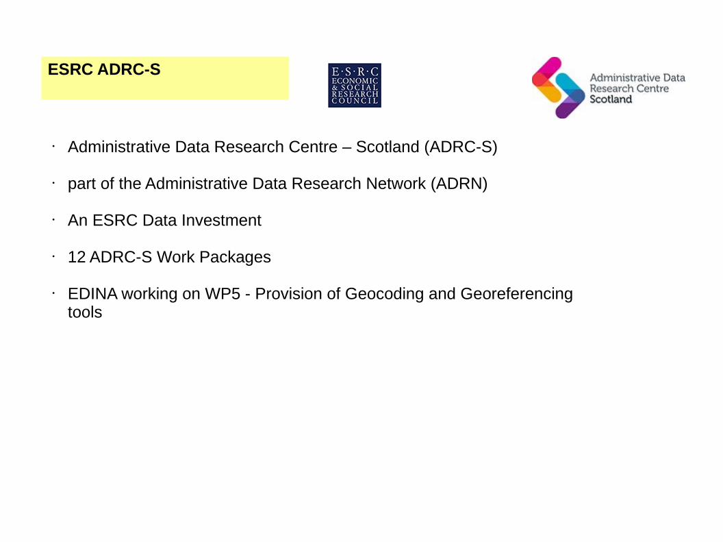
• Administrative Data Research Centre – Scotland (ADRC-S)
• part of the Administrative Data Research Network (ADRN)
• An ESRC Data Investment
• 12 ADRC-S Work Packages
• EDINA working on WP5 - Provision of Geocoding and Georeferencing tools

What and Why?
• Prof(s) Chris Dibben and Jamie Pearce from UoE GeoSciences
• Effects of past environmental conditions on (longitudinal) population cohorts
• Trains – where (and which populations) did they run alongside in the past and bring their air pollution
• Urban - did past populations live in predominantly urban or rural locales – were these same populations experiencing urbanisation
• Industry - where were particular types of (polluting) industry located?
• Greenspace and Bluespace – e.g. Parks and Water

Historic Maps – a record of past landscapes
• ADRC`s remit is (all) of Scotland.• Manual capture (digitising) of features from historic maps not going to
scale given resources available.• Chris and Jamie`s challenge to EDINA – is it possible to automagically
capture features from historic maps?• Historic maps in Digimap historic• For the purpose of this work we are using (higher quality) full colour scans
of historic maps provided by Chris Fleet @ NLS• Mainly been looking at 2 map series provided by NLS
• http://maps.nls.uk/geo/explore/#zoom=15&lat=55.9757&lon=-3.1799&layers=168
• http://maps.nls.uk/geo/explore/#zoom=15&lat=55.9757&lon=-3.1799&layers=10

Environment
• Linux (Ubuntu)
• Python (3)
• Virtualenv – isolated Python environments
• PyCharm Python IDE (Community Edition)
• OpenCV – Computer Vision / Image Processing / Image Analysis
• PostgreSQL - Datastore
• PostGIS – Spatial query (analysis) engine
• QGIS – Desktop GIS / PostGIS data viewer
• (a bit of) ArcGIS for ArcScan (Line vectorization)

OpenCV
OpenCV (Open Source Computer Vision) is a library of programming functions mainly aimed at real-time computer vision

Python Libraries used
• numpy - numpy (array) data structures central to all other libraries where we are manipulating image / raster datasets via python
• cv2 - python interface to OpenCV
• Shapely – (GEOS based) package for manipulation and analysis of planar geometric objects.
• Fiona – (F)ile (i)nput (o)utput (n)o (a)nalysis. An alternative API to OGR to access and write vector GIS datasets e.g. Shapefiles / GeoJSON.
• Rasterio – Raster (i)nput (o)utput. Rasteio is to raster GIS datasets as Fiona is to vector GIS datasets.
• Snaql – Keep (templated) SQL query blocks seperate from python code and render (with context) the query block when needed.
assuming PostGIS, if you add in a map renderer like mapnik, then this lot gives you everything needed to do geospatial data analysis (raster and vector), data conversion, data management and map automation.
Python OpenCV Demo
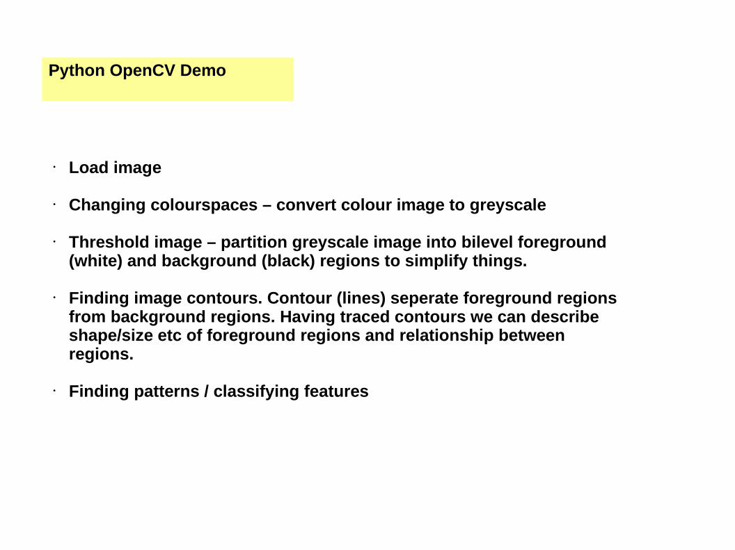
• Load image
• Changing colourspaces – convert colour image to greyscale
• Threshold image – partition greyscale image into bilevel foreground (white) and background (black) regions to simplify things.
• Finding image contours. Contour (lines) seperate foreground regions from background regions. Having traced contours we can describe shape/size etc of foreground regions and relationship between regions.
• Finding patterns / classifying features

Apply similar processes tohistoric maps to extract geographic features
(1) Water features (Bluespace)
(2) Railways
(3) Urban Form / Change

#15759 – extract 'bluespace'(1) Water features (Bluespace)
Rivers / Canals / inland water shown as blue lines or stippled blue areas.
Find contours – each stipple mark / line forms a contour
Threshold to isolate bluepixels
Contours form a hierarchy. Parents that hold child contours are water regions.

Method 2
Process breaks down when water regions are not entirely bound by blue lines or broken by other features (bridges).
So (alternative method) find every individual stipple and then forming groups of these gives water regions.
Apply either of these methods of capturing blue stippled regions to other stippled regions e.g. green stippled regions (parks - greenspace)

Change - old Edinburgh quarries change to shopping centres or from bluespace to greenspace!
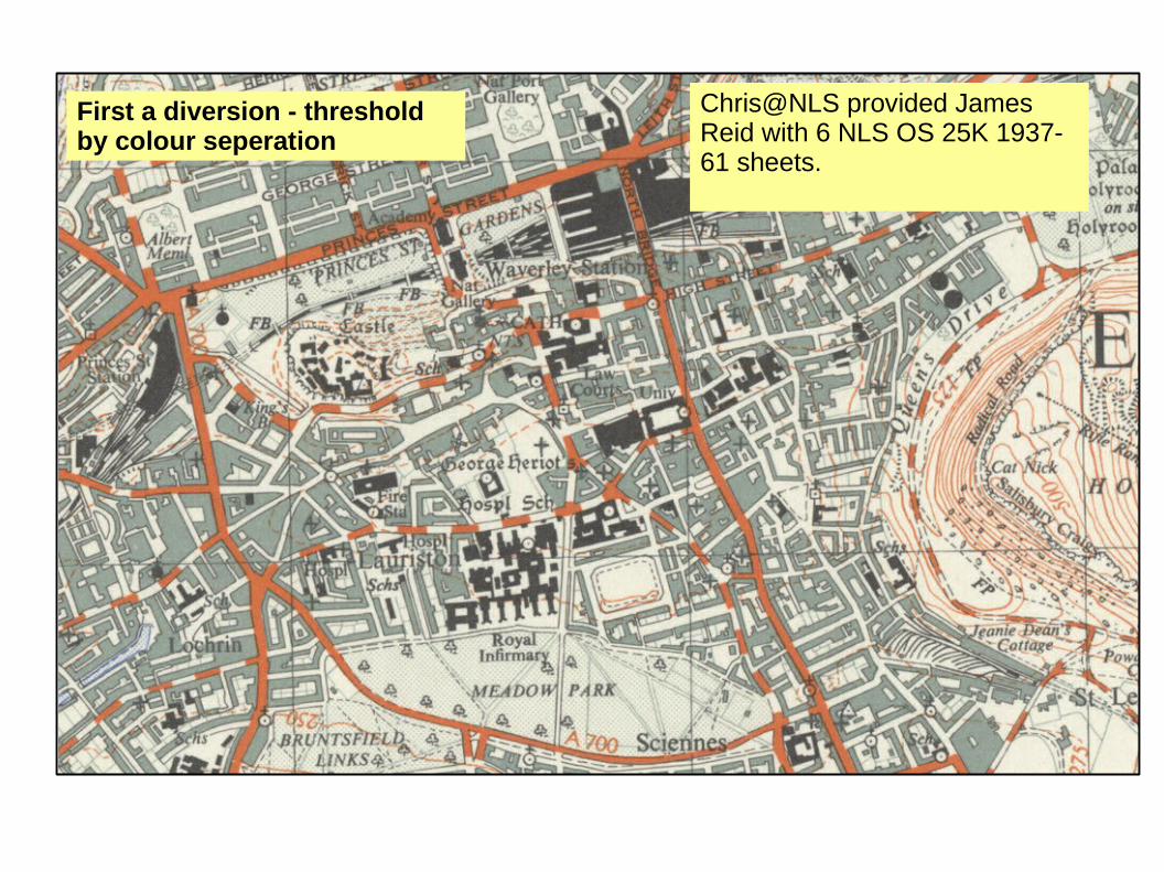
Chris@NLS provided James Reid with 6 NLS OS 25K 1937-61 sheets.
First a diversion - threshold by colour seperation
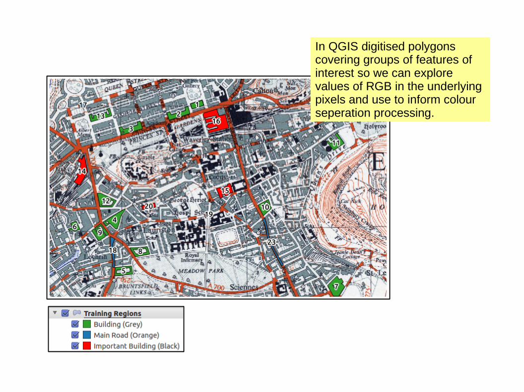
In QGIS digitised polygons covering groups of features of interest so we can explore values of RGB in the underlying pixels and use to inform colour seperation processing.
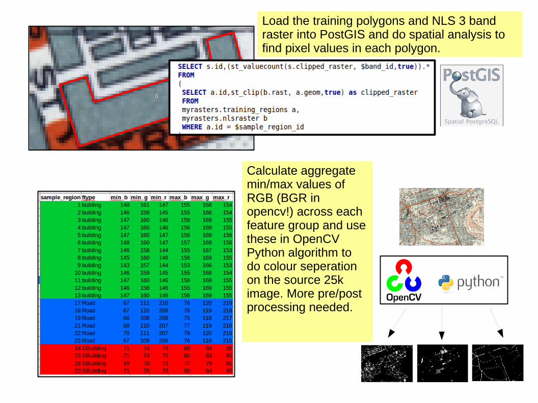
Load the training polygons and NLS 3 band raster into PostGIS and do spatial analysis to find pixel values in each polygon.
Calculate aggregate min/max values of RGB (BGR in opencv!) across each feature group and use these in OpenCV Python algorithm to do colour seperation on the source 25k image. More pre/post processing needed.

Pixels corresponding to (grey) buildings
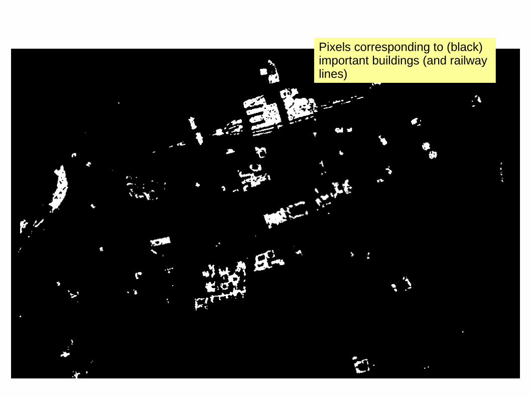
Pixels corresponding to (black) important buildings (and railway lines)
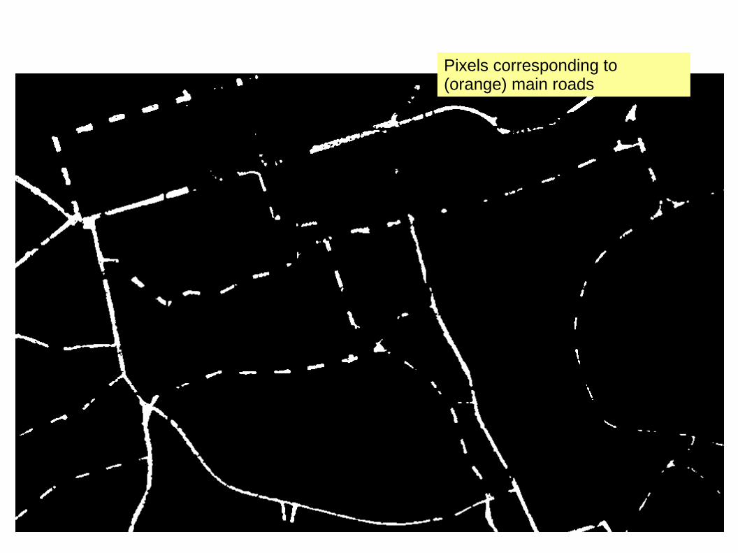
Pixels corresponding to (orange) main roads

(2) Extracting Railways
Source 1:25,000 NLS Historic Map “black” pixels extracted after running colour seperation process. Isolates dashes in railway lines (but also text/buildings)
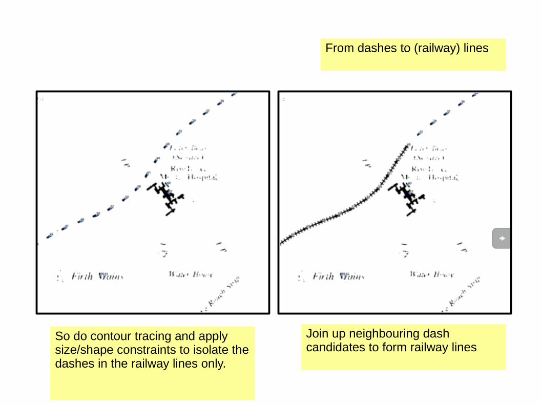
From dashes to (railway) lines
So do contour tracing and apply size/shape constraints to isolate the dashes in the railway lines only.
Join up neighbouring dash candidates to form railway lines

Complications…Process needs refined to cope with noisier, more complicated regions of the map
Not helped that some small buildings exhibit similar size/shape characteristics as dashes in railway lines.
A refinement might be to introduce a look-ahead constraint that minimises change in line direction as candidates are grouped since railway lines don`t make sharp 90 degree turns.
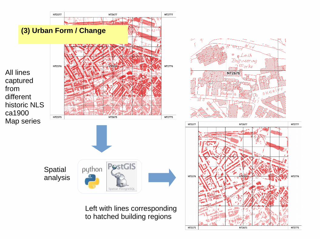
All lines captured from different historic NLS ca1900Map series
Left with lines corresponding to hatched building regions
Spatial analysis
(3) Urban Form / Change
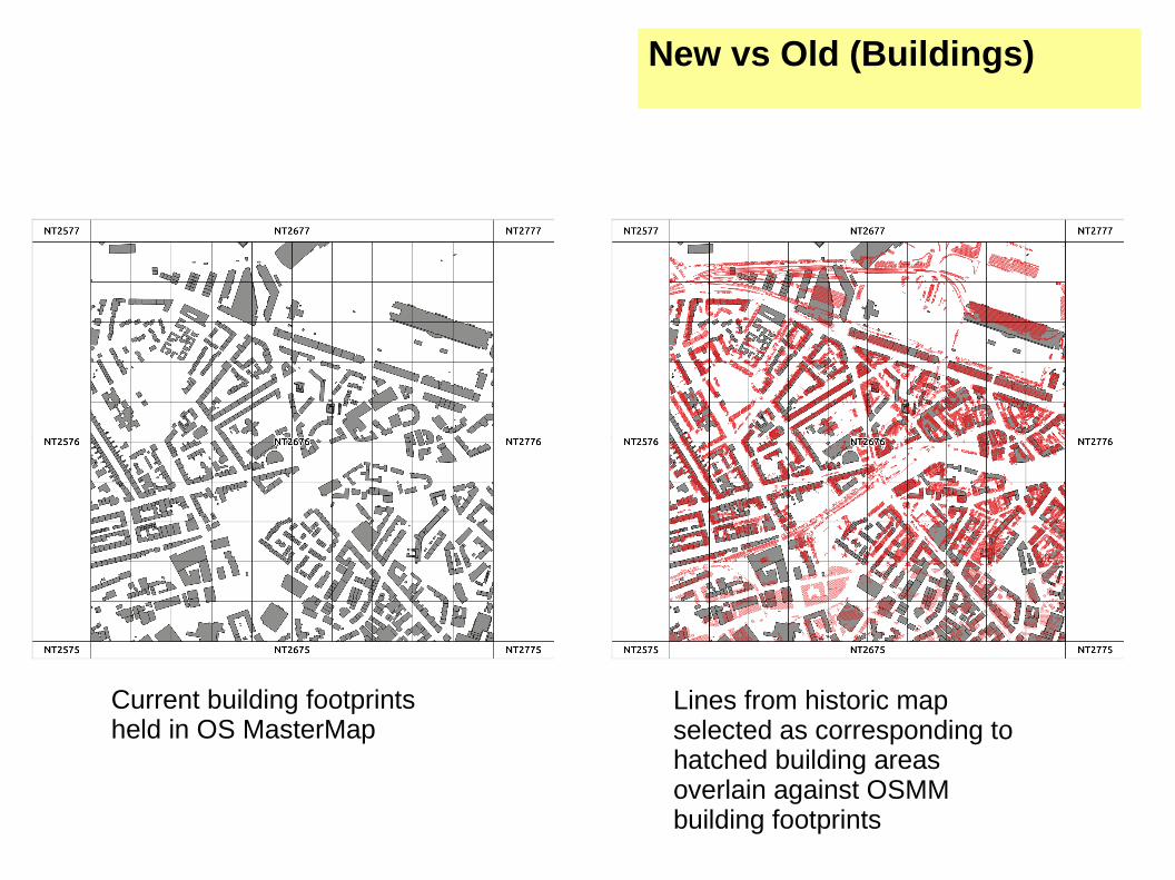
Current building footprints held in OS MasterMap
Lines from historic map selected as corresponding to hatched building areas overlain against OSMM building footprints
New vs Old (Buildings)
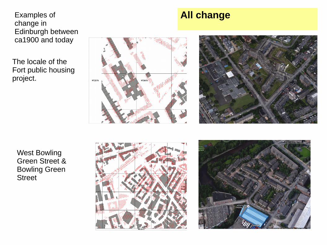
The locale of the Fort public housing project.
West Bowling Green Street &Bowling Green Street
Examples of change in Edinburgh between ca1900 and today
All change
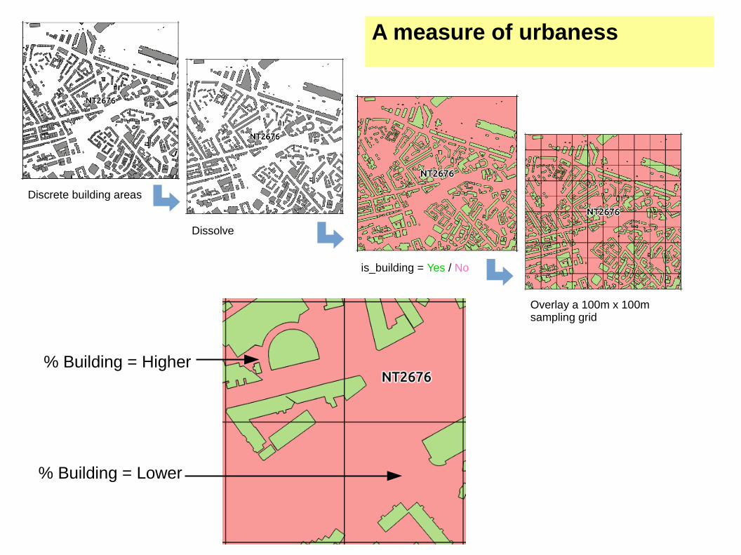
Discrete building areas
Dissolve
is_building = Yes / No
Overlay a 100m x 100m sampling grid
% Building = Higher
% Building = Lower
A measure of urbaness
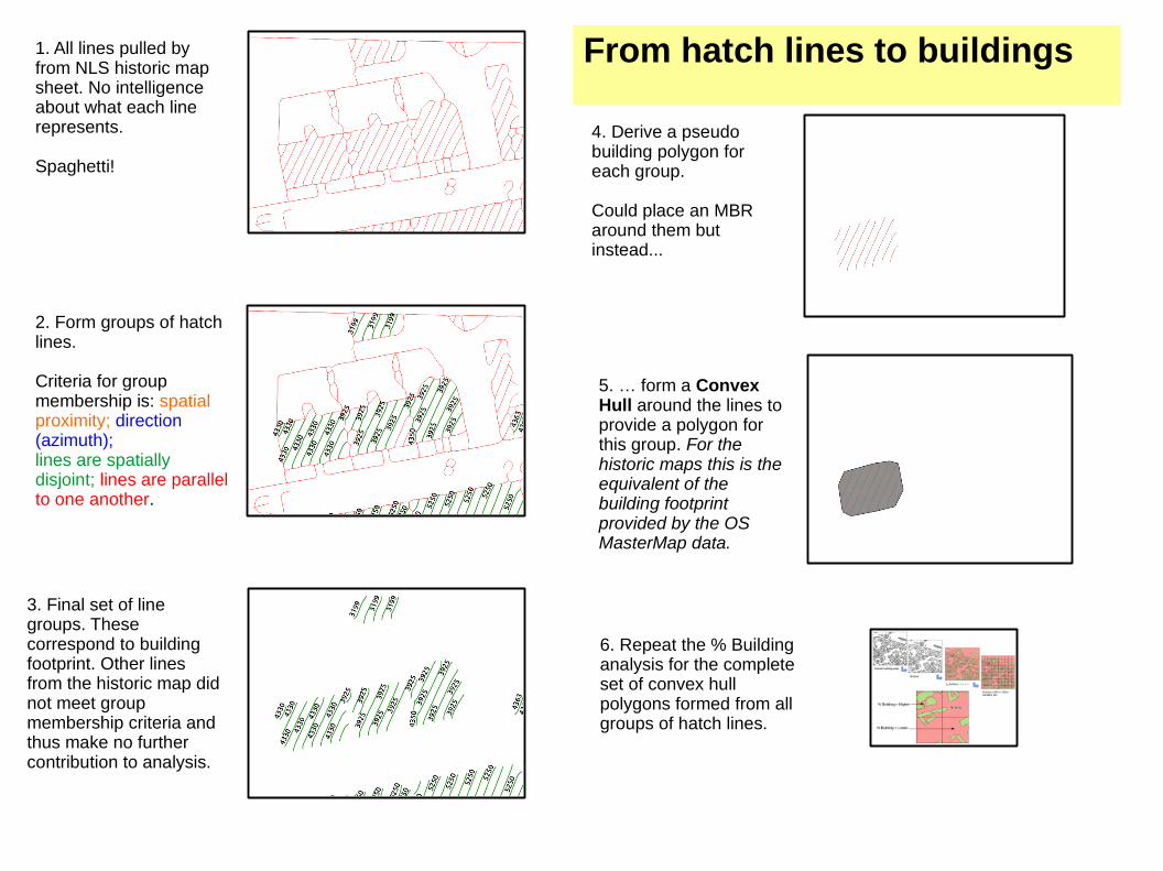
1. All lines pulled by from NLS historic map sheet. No intelligence about what each line represents.
Spaghetti!
2. Form groups of hatch lines.
Criteria for group membership is: spatial proximity; direction (azimuth);lines are spatially disjoint; lines are parallel to one another.
3. Final set of line groups. These correspond to building footprint. Other lines from the historic map did not meet group membership criteria and thus make no further contribution to analysis.
4. Derive a pseudo building polygon for each group.
Could place an MBR around them but instead...
5. … form a Convex Hull around the lines to provide a polygon for this group. For the historic maps this is the equivalent of the building footprint provided by the OS MasterMap data.
6. Repeat the % Building analysis for the complete set of convex hull polygons formed from all groups of hatch lines.
From hatch lines to buildings
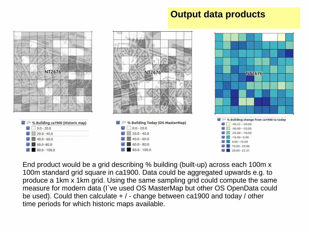
End product would be a grid describing % building (built-up) across each 100m x 100m standard grid square in ca1900. Data could be aggregated upwards e.g. to produce a 1km x 1km grid. Using the same sampling grid could compute the same measure for modern data (I`ve used OS MasterMap but other OS OpenData could be used). Could then calculate + / - change between ca1900 and today / other time periods for which historic maps available.
Output data products
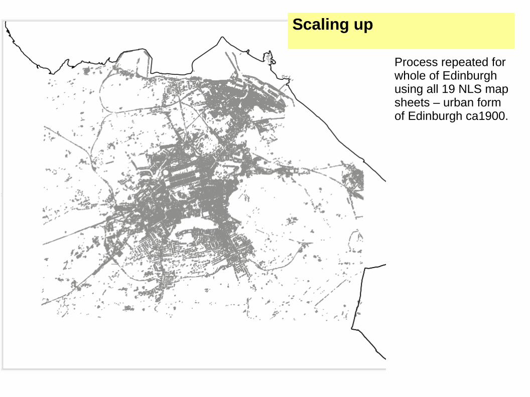
Process repeated for whole of Edinburgh using all 19 NLS map sheets – urban form of Edinburgh ca1900.
Scaling up
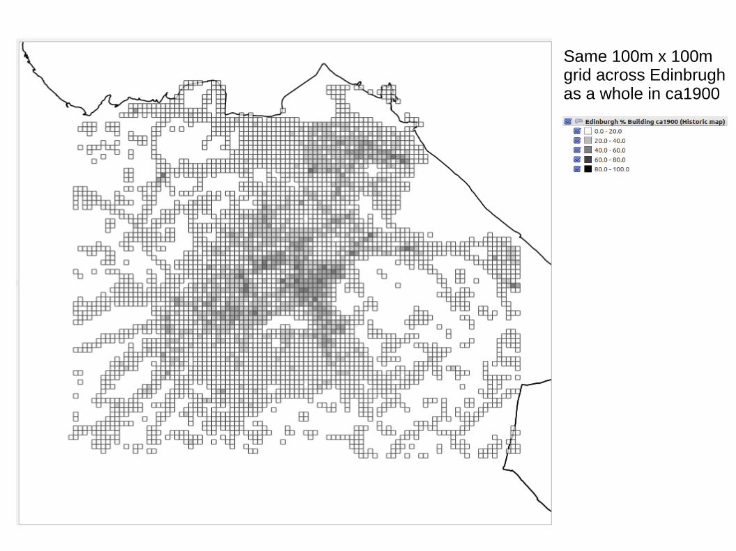
Same 100m x 100m grid across Edinbrugh as a whole in ca1900


