Effective Demand in the Recent Evolution of the US Economy1
by
Julio López-Gallardo
Universidad Nacional Autónoma de México
Luis Reyes-Ortiz Université Paris 1, Panthéon-Sorbonne
June 2011
1 Julio López Gallardo,Faculty of Economics, Universidad Nacional Autónoma de México Universidad 3000, Edificio de Oficinas Administrativas 2, 04510, Ciudad Universitaria, México; [email protected]. Luis Reyes, Université Paris 1, Sorbonne, Maison des Sciences Économiques, 106-112 Boulevard de L’Hôpital, 75647 Paris cedex 13; [email protected]
The Levy Economics Institute Working Paper Collection presents research in progress by Levy Institute scholars and conference participants. The purpose of the series is to disseminate ideas to and elicit comments from academics and professionals.
Levy Economics Institute of Bard College, founded in 1986, is a nonprofit, nonpartisan, independently funded research organization devoted to public service. Through scholarship and economic research it generates viable, effective public policy responses to important economic problems that profoundly affect the quality of life in the United States and abroad.
The recent crisis brought back to a central stage the teachings of Keynes, and the critical role of
effective demand as a determinant of the evolution of capitalist economies. To mitigate the dire
consequences of the crisis, economic authorities all around the world were compelled to sustain
demand with expansionary policies, including deficit spending. Besides, mainstream academic
economists were forced to temporarily put into a shelf almost everything they had been teaching
during the last thirty-odd years. In this new situation, the overall view of Michal Kalecki, as
well as the post Keynesian school inspired on the two founding fathers of the principle of
effective demand, also regained some public prominence.
In this paper, we use the principle of effective demand to study empirically the evolution
of the US economy before the eruption of the crisis, using modern econometric procedures. Our
general objective is to show that its evolution can be fully explained by the behavior of demand-
side variables. We also test some specific hypotheses about the role of fiscal and monetary
policies and of income distribution in shaping output and employment. Thus, in our study we
hope to answer with an alternative vision and with solid evidence to today’s dominant view,
which attempts to explain the evolution of capitalist economies on the basis of so-called
Dynamic Stochastic General Equilibrium models.
Understanding the significance of the monetary situation and policies is obviously
important in any study about the recent US development, where financial sophistication has
developed at a phenomenal speed. A crucial point here is whether monetary policy can have a
lasting influence on the level of output and employment, against the claim from mainstream
economists who refute this possibility. Keynes maintained that, except during particular
circumstances, availability of credit and low rates of interest would stimulate the pace of
investment and expand effective demand, and conversely. In contrast, Kalecki did not give
much importance to monetary conditions and policy. The significance of money and of the
interest rate, as well as the difference of opinions between Keynes and Kalecki over this issue, is
something that can be put to test, and which we put to test in this paper.
Fiscal policy is another type of intervention the forebears as well as supporters of the
principle of effective demand strongly recommend. On the contrary mainstream economists
3
reject it even more vocally that any other type of government involvement. Keynes and Kalecki
had rather similar views on this issue, except for one particular point, about the effect of
taxation of profits, where they disagreed. In this paper we put to test the role of fiscal policy, as
well as the difference of opinions between these two great thinkers.
Finally, Keynes and Kalecki viewed income distribution as an important determinant of
effective demand and output. In the General Theory, the former claimed: “To suppose that a
flexible wage policy is a right and proper adjunct of a system which on the whole is one of
laissez faire, is the opposite of the truth” (Keynes 1964 269). However, he thought, at least in
this book, that upon an increase in employment, real wages would have to drop1. Kalecki, on the
other hand, claimed that a higher real wage and higher wage share does expand demand, and
with it output and employment.
The above-mentioned are the hypotheses we want to explore in the present work. It is
beyond our objectives to develop an overall study of the US economy. However, since output is
our main variable of interest, we specify a general model to explain this variable. Besides,
readers will probably recognize the points we study have been at the center of the economic
debate for several decades. As said, different schools of thought give different, and even
contradictory, answers to the issues under consideration. An additional investigation of these
questions, underlining the empirical side of the matter and using modern econometric
techniques, may not therefore be redundant.
Some Words on Method and Brief Review of the Literature
Before continuing with our analysis, we shall say a few words about the econometric method we
follow in this paper. This is important for evaluating the robustness of the empirical results of
our econometric work. Afterwards, and considering this methodological discussion, we consider
a brief sample of previous studies on the issues we deal with in the present paper.
There is an important controversy among econometricians about the most satisfactory
procedure for empirical modeling. In a recent survey, Colander (2009), contrasts two alternative
perspectives in empirical macroeconomics. He distinguishes on the one hand what he calls the
1 This hypothesis was based on Keynes’s acceptance of the principle of decreasing marginal returns in the short run. Afterwards, and in the light of empirical evidence, he recanted from his previous opinion, and recognized that higher employment could be accompanied by an increase in the real wages (Keynes 1939).
4
“European perspective”, based on “the general-to-specific Cointegrated Vector AutoRegressive
(CVAR)” approach; and on the other the currently dominant “Dynamic Stochastic General
Equilibrium (DSGE) models”. However, as Spanos (2009) has pointed out, the latter one can be
“… better described as a Pre-Eminence of Theory standpoint, where the data are assigned a
subordinate role broadly described as quantifying theories presumed adequate. In contrast, the
European general-to-specific CVAR perspective attempts to give data a more substantial role in
the theory-data confrontation and is more accurately described as endeavoring to accomplish the
goals accorded by sound practices of frequentist statistical methods in learning from data”2.
In our econometric work, we shall follow what the latter author calls “a probabilistic
approach to econometrics” (Spanos, Ibid). This approach stresses the use of statistically
adequate models as the basis of drawing reliable inferences. The term statistically adequate
refers to the validity of the probability and the statistical assumptions underlying the estimated
model. The foundation of this approach is a purely probabilistic construal of the notion of a
statistical model. This is considered to be a set of internally consistent probabilistic assumptions
aimed at capturing the statistical information in the data (chance regularity patterns). Economic
theory suggests the potential theoretical relationships and the relevant data. However, the
statistical model is specified by viewing the observed data as a realization of a generic vector
stochastic process with a probabilistic structure that would render the observed data a truly
typical realization thereof. Thus, we distinguish between the structural model, based on
substantive subject matter information, and the statistical model, chosen to reflect the systematic
statistical information contained in the particular data. The structural and the statistical models
will coincide when we can give a satisfactory, and sufficient for the purpose, economic
rationalization to the latter one. When this is not the case, we will need to reformulate
(reparameterize/restrict) an estimated well-defined statistical model to arrive at a structural
model.
The success of econometric modeling depends on how correct the postulated
assumptions are in capturing the statistical information in the data. Thus, in this approach,
2 Readers interested in the confrontation between alternative approaches to econometrics, are referred to Juselius and Franchi (2007), who thoroughly test Ireland's (2004) canonical DSGE model. The authors find that most inferences from this work may be misleading. When confronted with the data at hand the probabilistic and statistic assumptions underlying the model should be rejected.
5
misspecification testing plays a fundamental role to ensure the statistical adequacy of the model
and the reliability of the inferences based on such a model. This is because all statistical
inferences will be misleading unless the probability and the statistical assumptions of the
estimated model are valid.
Let us now review a small sample of applied works related to ours. We may disagree
with theoretical arguments underpinning the works we discuss, or with the results the authors
infer from their work. However, we have only cared about the statistical ‘validity’ of their
deductions by critically assessing their claims.
To start with, Blanchard and Perotti (2002) study the dynamic effects of government
spending and tax shocks on the US post-war economy. Their main conclusions are that 1)
whenever public spending increases, output moves in the same direction (the opposite happens
with net taxes) and 2) multiplier effects are close to unity. An increase in public spending
increases personal consumption (crowding in), but it also reduces private investment (crowding
out).
Laramie, Mair, Miller and Stratopoulos (1997) study the direct impact of taxes on profits
and private investment in the US for the period 1980-1993 on a quarterly basis. Their aim was
to prove Kalecki’s argument that taxes on corporate income do not necessarily depress private
investment, with a reduced form investment function. Their main inferences were that 1)
increases in taxes to corporate income, if paid through a decline of personal savings, may not
have an impact on profits. Besides, if such increase is accompanied by purchases of government
infrastructure or by transfers to the unemployed, it may increase after-tax profits, resulting in
new investment. 2) It is possible to stimulate investment with a minimum impact on the budget
deficit, satisfying at the same time income distribution goals.
All in all, we consider the results from Laramie et al. more reliable, because they test for
the statistical and probabilistic assumptions of their estimates, which is not the case for the
Blanchard and Perotti paper.
We discuss now a small sample of papers dealing with the effects of money and
monetary policy.
The first paper we consider is by Fair (2005), who conducts a full macroeconometric
model for the U.S. economy. One of the system’s equations is a two-stage least squares
6
regression for the three-month Treasury bill rate as dependent variable for the period 1954-2002
on a quarterly basis. This short-term interest rate is a function of price changes, unemployment,
the change in money supply and a dummy for the early Volcker period (1979:4 to 1982:3). Fair
infers: “The net effects of, say, a decrease in r [the interest rate; JL and LR] on the U.S. output
and the price level are positive. Output increases because there is an increase in the demand for
domestically produced U.S. goods, and the price level increases because of the increase in
demand and the depreciation of the dollar”(p. 659). Of the interest rate’s determinants, only
unemployment has a negative effect on it. The short-term interest rate equation is one of many
interrelated macroeconomic variables of the system, and the influence of the interest rate on
output is only seen, indirectly, through a stochastic simulation procedure. This procedure
consists of a set of estimations of average ‘variances’ between actual against predicted values of
four macroeconomic fundamentals (real GDP, the short-term interest rate, private non-farm
deflator and inflation) under different scenarios (no rule, modified rules and with tax rule).
Fair’s bottom line is: interest rate rules reduce output and price variability, thus monetary policy
is effective.
In another paper, Lown and Morgan (2006) estimate a VAR model using real GDP, the
federal funds rate, loans and standards. The last variable represents non-price lending terms,
which they take from a survey (discontinued through 1984:1-1990:2). Their models run from
1968:1 to 2000:2 on a quarterly basis, omitting the period where the standards variable was
discontinued. They estimate several combinations of periods and variables to control for
robustness of the signs and sizes of the estimated coefficients. In particular, they found that real
GDP is negatively affected by the interest rate (price lending terms) and standards (non-price
lending terms), as well as positively affected by loans. Standards, they argue, seem to weigh
more.
With a similar approach, Bayoumi and Melander (2008) estimate a model under the
assumption that loan standards depend negatively on bank capital-asset ratio (CAR) and
positively on lagged standards (all as percentages of GDP). Changes in credit in turn depend
negatively on loan standards and on changes in the interest rate, and positively on changes in
income. Spending (both on consumption and investment) depend positively on credit (and its
lags), on income. Finally, CAR depends on one period-lagged GDP. Their single equations
7
contain MA terms or are estimated by 2SLS (spending equation) for inconsistent periods. As the
authors themselves recognize, they do not model any economic policy response to a financial
shock.
One of the previously-mentioned authors co-authored a more recent study (Bayoumi and
Darius 2011). The authors broaden the scope of the analysis, to examine the role of credit
markets in the transmission of U.S. macro-financial shocks, using a financial conditions index
(FCI). They estimate a vector auto regression (VAR), using information from the Senior Loan
Office Survey (SLOS).Their conclusion is worth quoting in length: “Our baseline specification
confirms the importance of the SLOS in predicting output and the results are relatively
independent of whether the credit variable is the small- and medium- sized firm survey rather
than the large company... Examining the impulse responses of real GDP, economic activity is
relatively sensitive to lending standards, particularly in the longer-term…. A one standard
deviation shock is associated with a highly-significant 0.3 percent decline in output after one
year, rising to 0.4 percent after 2 years. By contrast, the 3-month LIBOR rate has a much more
temporary and only marginally significant impact on output. A one-standard deviation shock
peaks at 0.15 percent after 3 quarters and has minimal impact after 2 years. Of the other asset
prices, the investment grade spread, high-yield spread, and equity prices all build gradually over
time, while the real effective exchange rate follows LIBOR in having only a temporary effect….
Variance decomposition finds that the SLOS survey is the main private sector financial indicator
explaining changes in output and dominates all other variables over time” (Bayoumi and Darius
2011 p. 8).
All in all, these studies seemingly support the hypothesis of a real effect of monetary
variables on output. Anyway, a problem common to the three of these papers is that the authors
do not test for the probability and statistical assumptions of their estimated models.
Let us finally consider some works studying the association between output (or other
macro variables), and income distribution. By the way, many contemporary authors, inspired by
the work of Kalecki, nonetheless propose the idea that a wage fall may stimulate demand and
employment. Thus they have coined the notions of profit-led and wage-led regimes. The former
means a higher profit-share stimulates output and employment, and conversely for the latter.
8
The first paper we consider is by Stockhammer and Onaran (2004). They modeled the
growth rate of the capital stock, the output gap, the profit share of the business sector, the
national unemployment rate and productivity growth. The method is structural VARs for the
US, the UK and France with semi-annual (OECD Economic Outlook) data for the periods
1970:1–1997:2 (UK), 1966:1–1997:2 (US) and 1972:1–1997:2 (France). They found that these
economies are wage-led.
Naastepad and Storm (2007) estimated simple linear regressions of investment and
exports functions for eight OECD economies for the period 1960–2000. They thus studied
Japan, US, France, Germany, Italy, Netherlands, Spain and UK, with annual (OECD) data.
Comparing signs and sizes of the estimated coefficients they infer that Japan and the US are
profit-led, whereas the six European economies they study are wage-led.
A third study is by Hein and Vogel (2008). They estimate single equation error
correction models for the period 1970–2005 on an annual basis. They found that growth in
France, Germany, UK and US is wage-led, whereas growth in Austria and the Netherlands is
profit-led.
Finally, Barbosa-Filho and Taylor (2006) analyzed the relationship between effective
demand and income distribution for the US economy, using a VAR(2) model. This includes
capacity utilization and the wage share; as well as private consumption, private investment,
government expenditure and net exports (the last four variables expressed as a share of potential
output). Their period under analysis is 1948-2002 on a quarterly basis. Their results show a
negative association between the wage share and capacity utilization; and thus between the
wage share and output.
As we can see, results differ among different authors about the effect of a rising wage
share on effective demand and output (or accumulation). However, we cannot accept their
inferences without qualification, because the authors do not always provide misspecification
tests, which in the spirit of our work are indispensable to assess the statistical validity of their
findings3.
3 There is another problem with the previously reviewed works. They all normalize the variable of interest by either capital or potential output. Now, this may have been the most appropriate procedure to study the dynamic stability conditions of the neo-Kaleckian Saving-Investment model originally proposed by Bhaduri and Marglin (1990) and Bowles and Boyer (1995). However, it seems much less adequate for econometric work, because
9
Anyway, taking stock of the previous discussion, we can now advance to the empirical
part of our research.
The Model
To adequately test the hypotheses we want to explore in this paper, we would need a detailed
macroeconometric model. Since this is beyond our possibilities, we have estimated a Vector
Auto Regression (VAR) specification. We chose this method because most variables are
interrelated and because it would not be correct to assume a priori which of them are
endogenous and which are exogenous. We also use system-based cointegration methods
(Juselius, 2006). These methods allow us to deal with the non-stationary nature of economic
time series. Taking as the basis a VAR model, we then estimate an error correction model
(ECM) and a cointegrated Structural VAR model (SVAR), which we use to carry out Impulse-
Response analysis. The use of different methodologies allows us to confirm the robustness of
our empirical results and the validity of our theoretical hypotheses.
Our main variable of interest is US GDP. As said, we want to study only if and how,
fiscal, monetary and distribution variables affect GDP. However, to guarantee substantive
adequacy of our model, we must consider all the variables that are likely to affect GDP, as well
as their interactions. Thus, we need a general specification, within which to nest the fiscal
policy, monetary and factor share variables. Therefore, we start from the National Accounts
identity slightly adjusted. Let Y stand for output, C private consumption, I private investment,
and J the trade balance (i.e. net exports). G is government expenditure on goods and services.
Y = C+ I + J + G (1)
We now have to find out which are the most basic factors controlling the right-hand side
variables. Unfortunately, however, we have a limited range of choice because we must save
enough degrees of freedom to carry out the estimation and misspecification tests. Besides, lack
measures of capital or potential output are difficult to come by, and are in general not too reliable, which affects all the resulting inferences.
10
of adequate information will force us to use variables that are only imperfect proxies for our
theoretical variables of interest. We now explain how we deal with this situation4.
We shall assume the trade balance (J) depends on domestic output, on external output
(Y*), and on the wage share. This is because the exchange rate depends on (and moves in
opposite direction than) the share of wages in value added for a given nominal exchange rate
(López and Perrotini 2006).
We assume private consumption and private investment depend on income and on the
share of wages in the value added. We also assume that both private consumption and
investment depend on private credit outstanding (C) and on the interest rate (R). As we know,
over the last years, and until the financial crisis imploded, a dramatic rise in private credit
outstanding occurred, and we have to consider this important new factor5.
Finally, we break up government spending on goods and services according to the source
from which it is financed. Thus Hand O are taxes on corporate profits (H) and Other
Government Revenues (O). It would have been preferable to separate the budget deficit from net
taxes from persons. However, the actual budget deficit, for well-known reasons, is pro-cyclical,
and we did not find a satisfactory variable measuring the discretionary budget deficit6.
Therefore, we can reduce (1) as follows:
Y = C (w, Y, C, R) + I (w, Y, C, R) + J (Y, Y*, w) + H + O (2)
where R is the 3-month Treasury bill rate7. Simplifying again, our model will be
specified as:
Y = Y (w, Y*, C, R, H, O) (3)
where the right-hand side variables are also endogenous.
We begin the modeling exercise with a brief description of the data8. The sample is on a
quarterly basis, and it runs from 1980 to 2008(3). All monetary variables have been brought to
4 Note, we tried many models, with different information sets. We finally selected the model we present below because it was the best one from the statistical point of view. That is, it was subjected to, and was not rejected by, a large battery of misspecification tests. 5 By the way, we also tried to have variables reflecting private wealth into our specification, but we did not find a statistically valid model including this variable. 6 We also estimated models where we split the (actual value of) budget deficit from net taxes from persons, but we confronted the problem of lack of degrees of freedom. Besides, the resulting estimates were not statistically valid. 7 We tried different interest rates until we could identify one that resulted in a solid statistical specification.
8 See the Appendix for the model data source.
11
2000 prices. In Figure 1 below we plot each variable and GDP. This will give us a first informal
hint on how each one of the selected variables changed during the period, as well as how they
may be connected. To simplify visual inspection of their possible association we show on the
left-hand panel the seasonally adjusted variables, and the variables in deviation from their trend
on the right-hand panel.
Figure 1. GDP and Variables of the Model
Source: See Appendix.
1980 1985 1990 1995 2000 2005
-0.25
0.00
0.25A
GRAPH 2. GDP AND VARIABLES OF THE MODEL
Y
Y*
B B'
1980 1985 1990 1995 2000 2005
-0.05
0.00
0.05 A´
Y_T
Y*_T
1980 1985 1990 1995 2000 2005
-0.25
0.00
0.25
0.50 C
Y1980 1985 1990 1995 2000 2005
-0.05
0.00
0.05C´
W_T
Y_T
1980 1985 1990 1995 2000 2005
-0.25
0.00
0.25
0.50 D
H
Y
1980 1985 1990 1995 2000 2005
-0.25
0.25D´
H_T
Y_T
1980 1985 1990 1995 2000 2005
5
15
Y
R
W
1980 1985 1990 1995 2000 2005
-5
0
5 Y_T
R_T
1980 1985 1990 1995 2000 2005
-0.25
0.00
0.25
0.50 EE
OY
1980 1985 1990 1995 2000 2005
-0.05
0.00
0.05 E´O_T
Y_T
1980 1985 1990 1995 2000 2005
-0.25
0.00
0.25
0.50 F
C
Y
1980 1985 1990 1995 2000 2005
-0.05
0.00
0.05 F´
C_T
Y_T
12
As we see in the figure from the output series, the aftermath of the crisis at the beginning
of the eighties was hard to overcome. Only after the first half of the same decade output started
growing steadily. The nineties started with a mild but lasting recession and a stock market boom
fueled recovery, followed by another recession the next decade. OECD output displays a similar
evolution as that of US output, except at the beginning of the nineties. The interest rate has
gradually decreased since the beginning of the eighties, with drastic falls during recessions,
increasing along most booms, with the important exception of the 1995-2000 stock market
boom. The share of wages in GDP did not worsen for workers immediately and as deep as
output during the 81-82 crisis, but from the beginning of the nineties on it has moved more pro-
cyclically.
Taxes on corporate income have become gradually and pro-cyclically more responsive to
fluctuations in GDP, whereas the budget deficit and taxes on workers (lumped together as other
budget revenues) do not present a clear trend. It must be noticed, however, that taxes on workers
represent a higher proportion on this series, thus that redistributive fiscal policy through taxes on
workers has changed drastically. Finally, credit availability showed a clear sensitiveness to
recuperation from the crisis of the early eighties, increasing more that output, but more so in the
recession of the beginning of the nineties. Its fluctuations have been milder since then but
following more or less the same pattern.
As shortly explained in the last two paragraphs, at first sight we can see a close positive
association between Y and Y* (panels A and A’); between Y and w (panel C’); between Y and
H (D’); between Y and C (F’); and probably also between Y and O (E’). The nature of the
association between Y and R is less clear. Anyway, at first sight the information suggested by
the figures support the notion that demand-side variables strongly influence the economy. More
13
specifically, they appear to validate Keynes’s conjecture about the importance of credit and the
interest rate, of Kalecki’s hypothesis regarding the expansionary role of the wage share, and of
Keynes’s and Kalecki’s hypotheses about the relevance of government expenditure, on demand
and output. But our econometric work will tell us whether this is actually the case.
From a statistical point of view, graphs of the variables suggest that all of them are non-
stationary, i.e. they have a trending mean; also their underlying density function seems to be
non-normal9. Unit root analysis of the series (not shown here) suggests that all series used in the
model have the same order of integration (all are I(1)). Provided we have a well-specified
model, we can test for cointegration via the Johansen procedure.
We estimated a VAR with quarterly data for the period 1980-2008(3). We included the
US GDP (Y), OECD GDP (Y*), private credit outstanding (C), profit-tax financed government
expenditure (H), other government revenues (O), the wage share (w), and the short-run interest
rate (R). All the variables, except the last two, are in logarithms. We found a statistically well-
specified equation, in a model including an unrestricted constant, four lags and four dummy
variables10. We included variable R as exogenous11.
After checking for misspecification and confirming that the model was not rejected by
individual-equation and vector misspecification tests, we checked for a long-run association
between our set of variables with Johansen’s cointegration test. The test suggests that up to five
9 We checked this with normality tests, which rejected normality for all the variables. Non-normality may be due to the presence of outliers. 10 These are for the following periods: 1982(1), 1987(1), 1993(1)-1994(1) and 2000(1). The first helped to correct normality problems for Y and Y*, in the middle of the 1981-1982 crisis. The second was used to ameliorate a sudden change in C occurred at such point in time. The third dummy was useful in accounting for drastic declines in w in the first quarters of ‘93 and ’94. The fourth one effectively eliminated normality problems in w, as well as in H. 11 We were unable to find a statistically adequate model with R endogenous. We believe this is because the interest rate is in fact policy-determined, and is not exclusively associated with the variables included in our model.
14
cointegration vectors can exist12, and we take the first one as implying the long-run association
between US GDP and its determinants13. This long-run vector is as follows:
y = 0.83 y* + 2.17 W + 0.14 c + 0.15 o + 0.11 h – 0.012 R (4)
where lower-case letters refer to the variable in logarithms. The vector misspecification
test statistics are displayed in Table 2 below.
Table 1. VAR Vector Misspecification Tests.
Test Statistics values
Vector AR 1-5 test : F(180,250) 0.99467 [0.5124]
Vector Normality test : Chi^2(12) 20.663 [0.0555]
Vector Hetero test : F(1050,231) 0.24489 [0.990]
Source: See text.
In words, we find that higher output is associated with higher OECD GDP, with a
higher share of wages in value added, and with higher government expenditure financed either
via higher taxes on profits or via higher other government revenues. Finally, a higher interest
rate is associated with lower output.
Since correlation does not imply causation, it is still necessary to study whether output is
indeed determined by the right-hand side of (4). Therefore, we carried out Granger causality
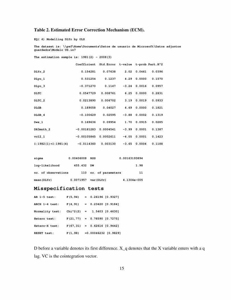
tests and found out that this is in fact the case. This is confirmed by the estimated Error-
Correction Model, which describes the short-run association between US GDP and its
determinants. Table 3 below shows the Error-Correction Model, where VC denotes the long-run
cointegration vector. Note that, in a multi-variate context, Granger causality of variable X on
variable ϑ is obtained when X is contained among the regressors in the equation for ϑ, or in the
cointegration vector, or both. 12 According to the corresponding test for stability of the vectors only two of them are stable. 13 This was not an a priori distinction between endogenous and exogenous variables; we estimated a valid VECM model and then we tested the validity of the restriction of the existence of an output equation.
D before a variable denotes its first difference. X_q denotes that the X variable enters with a q
lag. VC is the cointegration vector.
16
Finally, and to provide further evidence related to our previous findings, in this section
we make use of the SVAR methodology, using the cointegrated VAR model from the previous
section, and we conduct Impulse-Response Analysis.
We obtain the structuralized, contemporaneous effects, suggested by equation y = y(W,
y*, c, R, h, o) by imposing the appropriate restrictions in the matrices of the errors. We ensure
the validity of the previously imposed restrictions by means of a LR test, and we reach the
following estimates for the contemporaneous interactions14.
Table 3.
Estimated Contemporaneous Effects. Estimates of SVAR Parameters
STATISTICS ON AB MODEL PARAMETERS
PARAMETER COEFFICIENT STD.ERROR T-VALUE
Y-Y* 0.8071 0.0914 8.83
Y-H 0.0208 0.0055 3.78
Y-O 0.1063 0.0220 4.83
Y-C 0.0057 0.0422 0.14
Y-WS -0.4031 0.1187 3.40
OVER-IDENTIFICATION LR TEST CHI-SQUARED( 10 )= 22.04824 SIGNFICANCE LEVEL=
0.01486
Table 3 must be read as follows. The coefficients of each variable represent the short-run
contemporaneous responses resulting from a shock in the conditioning variables. Specifically:
the impact of government expenditure, foreign demand and the wage share are positive; and
14 Note, the variable R does not appear in the contemporaneous effects and in the Impulse Response Graphs, because it is taken as exogenous in our estimated VAR.
conversely, the interest rate has
statistically non-significant.
We can provide further evidence
making use of the typical simulation techniques known
based on the estimated VAR model and restricted to satisfy the cointegration r
IRA graphs are shown next:
FIGURE 2
Impulse R
Resp. of Y to Y*Resp. of
Resp. of
As we can see, shocks to
and to credit, have positive impacts
Let us now give an economic interpretation to our results
hypotheses that are the main object of our inquiry.
Firstly we notice that a higher share of wages stimulates demand and output in the short
and in the long-run. Note, the contemporaneous effect of the wage share rise on output is
negative, but turns positive afterwards
17
interest rate has a negative impact. Note the contemporaneous impact
We can provide further evidence on the effects of macroeconomic variables on output by
simulation techniques known as impulse response analysis (IRA
based on the estimated VAR model and restricted to satisfy the cointegration r
Response of the Structural Effects over Output
Impulse-Response to Shocks
Resp. of Y to Y*Resp. of Y to H Resp. of Y to O
Resp. of Y to C Resp. of Y to WS
shocks to the wage share, to government expenditure,
credit, have positive impacts on output and demand.
Let us now give an economic interpretation to our results, concentratin
hypotheses that are the main object of our inquiry.
we notice that a higher share of wages stimulates demand and output in the short
. Note, the contemporaneous effect of the wage share rise on output is
negative, but turns positive afterwards. From the second period onwards, the expansionary
the contemporaneous impact of credit is
variables on output by
as impulse response analysis (IRAs)
based on the estimated VAR model and restricted to satisfy the cointegration rank constraint.
utput
Y to O
, to world output
, concentrating on the
we notice that a higher share of wages stimulates demand and output in the short-
. Note, the contemporaneous effect of the wage share rise on output is
the expansionary
18
effect of a higher wage share on domestic demand more than offsets any possible recessive
impact on other demand items. This finding clearly supports Kalecki’s idea.
Secondly, we have found that higher government expenditure, either financed with
higher taxes on profits, or with other government revenues, stimulates demand and output. As
anticipated by Kalecki, the size of the impact depends on how government expenditure is
financed. To have an idea of the amounts involved, let us take into account that in 2007 US
GDP amounted to about 11,552.6 billions of chained (2000) dollars. Taxes on Corporate Profits
and Other Government Revenues were about 320.7 and 1,950 billion dollars, respectively. Now,
let us assume that in 2007 government expenditure had been US $100 (billions) higher than it
was. If that rise had been entirely financed taxing corporate profits, then the latter item would
have risen to US $420.7; i.e. an increase of 31% on its original value. Since the long-run
elasticity of GDP with respect to taxes on corporate profits is 0.11 (see eq. 4), that rise in
government expenditure would have brought about a long-run increase in GDP amounting to
3.35% (31 times 0.11); namely, of US $389 billion. On the other hand, if the US $100 (billions)
of extra government expenditure had been financed via other budget revenues, the latter would
have risen 5.9%. In the long-run output would have been US $104 billion higher. Thus,
according to our estimate, a much larger impact would take place if government expenditure
were financed taxing corporate profits than with other revenues.
Lastly, we have found that monetary conditions do affect demand and output, not only in
the short but also in the long run. Thus, our result contradicts the conventional view that denies
any long-run effect of monetary variables on the real economy. Contrariwise, it supports
Keynes’s hypotheses. Larger credit availability has a positive impact on demand, and a higher
interest rate tends to depress demand.
FINAL REMARKS
We may now summarize our findings. We have found full confirmation for the two Kalecki’s
hypotheses studied empirically in this paper. On the one hand, government expenditure financed
via taxes on profits has a positive effect of on demand and output. On the other hand, a shift
from profits to wages also expands demand. Let us delve a bit deeper into these two issues.
19
As a consequence of the depth of the current world financial crisis, public spending,
even deficit financed, has regained a place of honor in the arsenal of acceptable economic policy
instruments. This is hailed as a revival of Keynes and Keynesianism. Indeed, Keynes and
writers identified with the so-called Post-Keynesian school, emphasize the beneficial effect of
government expenditure, and of government deficit, when idle resources are abundant15.
There is much truth in the previous opinions. However, let us recall that Keynes was not
alone in underlining the use of government expenditure as a tool to fight unemployment. Also
Michal Kalecki, when he first put forward his version of the principle of effective demand, gave
a prominent place to government spending as an extra source of demand. He also added a twist
to that notion, claiming that even financing government expenditure with taxes on profits would
have an expansionary effect.
In our study we have been able to corroborate that government expenditure would raise
effective demand. We have also confirmed Kalecki’s specific hypothesis about the impact of
taxing profits to finance that expenditure.
Let us now discuss the second of Kalecki’s hypotheses, which we may relate to the
discussion that has taken place among Post-Keynesian economists on the so-called “wage-led”
and “profit-led” regimes. Whether a wage-share fall will stimulate demand or not in the short
run, depends on the balance between: a) its negative impact on workers’ consumption, and b) its
(supposed) positive effect on profits, investment and the trade balance. On the other hand, the
long-run effects of such a fall depend on the weight of the different determinants of investment
decisions. It also depends on how strongly investment impinges on the competitiveness of
domestic producers. The wage fall may raise profits in an open economy in the short run, but
may reduce demand and capacity utilization. The final result is ambiguous because profits and
capacity utilization are two arguments that affect investment decisions.
Our empirical results for the US economy suggest that in this country the shift from
wages to profits did indeed cause a short-term fall in effective demand. Besides, in the long run
demand and output also appear to be discouraged by this shift.
We may suggest the evolution has gone more or less along the following lines. Let us
consider a situation where a fall of the wage share improves the trade balance and profits in the
15 See especially Wray, 1998; and Arestis and Sawyer, 2003; as well as the bibliography cited therein.
20
short run, but depresses aggregate demand and output in the short run. Let us also assume a
simple investment function, where investment depends positively on only two arguments:
profits and capacity utilization. Let us finally assume the trade balance depends on the
competitiveness of domestic producers, which in turn depends on past investment. Then, if the
elasticity of investment with respect to profits is lower than its elasticity with respect to
utilization, a wage-share fall will have a short-run negative effect on output and employment.
Besides, that effect will persist because demand and supply factors come into play. On the one
hand, investment will be growing at a lower rate, dragging with it internal demand, due to the
demand (and capacity utilization) fall. On the other hand, the trade balance will not improve
much, and may even worsen, due to the adverse effect on competitiveness of a lower rate of
investment. This would be an example of what has been labeled in the previously cited literature
as a “wage-led” regime. We may infer from our empirical results that this regime may be the
one prevailing in the US economy.
Finally, let us say a few words about the monetary inferences arrived at from our
estimated model. Irrelevance theorems (old and new) hold that any attempt of the monetary
authorities to affect the aggregate demand and employment is doomed to failure. Worse, it can
have perverse effects on other macroeconomic fundamentals, mainly on inflation. Contrariwise,
Keynes’s main message was that monetary policy can be very powerful. He thought that open
market operations should be the driving factor in monetary policy, with the interest rate playing
a major role16. He also underlined the importance of banks, as the most important providers of
loans to the private sector17. Monetary authorities carry out this type of operation by inducing
private banks to substitute reserves for loans (expansionary policy), or to renew reserves
(contractionary policy). This will hold as long as there is a well-diversified financial system for
the portfolio adjustment (induced by open market operations) to be transmitted to the sector
with the longest maturity and is not exhausted in a simple short-term asset substitution.
On the other hand, and despite some confusion about Keynes’s position on the ability or
inability of the Central Bank to affect money supply in his writings, it is now clear that for him
16 In Keynes’s own words “The new post-war element of ‘management’ consists in the habitual employment of an ‘open-market’ policy (…). This method seems to me to be the ideal one” (Keynes 1930, Vol. II, pp. 206-207). 17 “[I]n general, the banks hold the key position in the transition from a lower to a higher scale of activity” (CWJMK, vol. 14, 222)
21
money supply may be actually affected18. Reductions in the interest rate directly increase banks’
reserves, and this in turn increases credit availability.
Needless to mention, today’s US financial system is extremely sophisticated and well
diversified, which implies that the importance of monetary policy is further reinforced in
comparison with what was the case in Keynes’s times. Our results suggest that the main
channels through which Keynes thought monetary developments affect the macro economy,
have indeed played a significant role in the recent evolution of the US economy. Low interest
rates and ample loan availability provided by banks surely explain a lot of its growth prior to the
crisis.
Other authors have argued that growing household indebtedness compensated for the
negative effects resultant form the shift from wages to profits, thus contributing to sustain
effective demand in the US economy19. We think our results confirm their opinions.
We now close. It is a fact of life that results arrived at in social sciences, and in sciences
in general, are never definite. As time goes by new information becomes available and new and
more powerful methods of analysis develop. Anyway, using the most complete set of
information at our disposal, and what we think is a rigorous (and demanding) method of
statistical analysis, we have reached what we believe are robust conclusions. In a nutshell, we
hope to have shown the effective demand approach is useful to explain the recent evolution of
the US economy. We have also proved, we hope, the main intuitions of their founding fathers,
Keynes and Kalecki, were essentially correct. We do not claim, of course, that what we found
for the US takes place in the same way in other advanced economies. The reaction of an
economy to shocks and to economic policy measures depends on its structure and institutions.
We would, nonetheless, suggest that the method we have used in this work might be useful to
study other national cases.
18 For a thorough review of the controversy in the interpretation of Keynes’ position regarding the ability of the Central Bank to affect money supply in A Treatise on Money and in The General Theory see Panico (2008). 19 See Cynamon and Fazzari (2008), Barba and Pivetti, 2009; and Fitoussi and Saraceno (2010).
22
REFERENCES
Arestis, Philip and Malcolm Sawyer. 2003. “On the Effectiveness of Monetary Policy and Fiscal Policy”. Working Paper 369. Annandale-on-Hudson, NY: The Levy Economics Institute of Bard College.
Barba A. and M. Pivetti. 2009. “Rising Household Debt: Its Causes and Macroeconomic
Implications–A Long Period Analysis.” Cambridge Journal of Economics Vol. 33, No.3, pp.113-37.
Barbosa-Filho, Nelson and Lance Taylor. 2006. “Distributive and Demand Cycles in the US
Economy -A Structuralist Goodwin Model”. Metroeconomica Vol. 57 Issue 3 pp. 389- 411. July.
Bayoumi, Tamim and Ola Melander, 2008. “Credit Matters: Empirical Evidence on U.S. Macro- Financial Linkages.” IMF Working Paper, Western Hemisphere Department. Bayoumi, Tamim and Reginald Darius. 2011. “Reversing the Financial Accelerator: Credit
Conditions and Macro-Financial Linkages.” IMF Working Paper. February.
Bhaduri, A. and S. Marglin. 1990. “Unemployment and the Real Wage: The Economic Basis for Contesting Political Ideologies.” Cambridge Journal of Economics 14: 375-93. Blecker R.A. 1999. “Kaleckian Macro Models for Open Economies.” In J. Deprez and J. T.
Harvey, eds., Foundations of International Macroeconomics. London: Routledge. pp. 116-49. Bowles S. and R. Boyer. 1995. “Wages, Aggregate Demand, and Employment in an Open
Economy: An Empirical Investigation.” In G. A. Epstein and M. G. Gintis eds., Macroeconomic Policy after the Conservative Era. Cambridge University Press.
Colander, D. 2009. Economists, Incentives, Judgement, and the European VAR Approach to Macroeconometrics. Economics. The Open-Access, Open-Assessment E-Journal, Vol. 3, September, http://www.economics-journal.org/economics/journalarticles/2009-9. Cynamon, B.Z., and S.M. Fazzari. 2008. “Household Debt in the Consumer Age: Source Of Growth—Risk of Collapse.” Capitalism and Society Vol. 3, Article 3. Fair, Ray. “Estimates of the Effectiveness of Monetary Policy.” 2005. Journal of Money, Credit
And Banking. No. 4, August, pp. 645-660. http://www.economics-journal.org/economics/journalarticles/2009-10.
23
Fitoussi, J.P., and F. Saraceno. 2010. “Europe: How Deep Is a Crisis? Policy Responses and Structural Factors behind Diverging Performances.” Taking a DSGE Model to the Data
Meaningfully. Vol.1, Issue 1, Article 17. Juselius, K. 2006. The Cointegrated VAR Model: Methodology and Applications. Oxford, UK:
Oxford University Press. Juselius, K and M Franchi. 2007. “Taking a DSGE Model to the Data Meaningfully.”
Economics Discussion Papers 2007-6. March. Kalecki, M. 1991 [1939]. “Money and Real Wages.” In J. Osiatynsky, ed, Collected Works of
Michal Kalecki. Vol. II. Oxford, UK:Oxford University Press. Kalecki, M. 1990 [1944]. “Professor Pigou on The Classical Stationary State”. In J. Osiatynsky
ed., Collected Works of Michal Kalecki. Vol. I, Oxford, UK:Oxford University Press. Kalecki, M. 1943.“Studies in Economic Dynamics.” In J. Osiatynsky ed., Collected works of
Michal Kalecki. Vol. II. Oxford, UK:Oxford University Press. Kalecki, M. 1997 [1956] “The Economic Situation in the USA as Compared With the Pre-war Period.” In J. Osiatynsky ed., Collected Words of Michael Kaleck., Vol. VII. Oxford,
UK:Oxford University Press. Keynes, J.M. 1930. A Treatise on Money. Two Volumes. London:Macmillan. Keynes 1973 [1937]. “The ‘Ex Ante’ Theory of the Rate of Interest.” The Economic Journal
pp. 215-23 in The Collected Writings, Vol. XIV, London: Macmillan. Laramie, A., Mair, D., A. Miller, and T. Stratopoulos. 1996-1997 “The Impact of Taxation on
Gross Private Non-Residential Fixed Investment in a Kaleckian Model. Some Empirical Evidence.” Journal of Post-Keynesian Economics (19:2) pp. 243-256. Winter.
Laski, K. and R. Römisch, 2001. “Growth and Savings in USA and Japan.” WIIW Working
Papers. No. 16. Vienna. López, Julio and Michaël Assous. 2010. Michal Kalecki. Series: Great Thinkers in Economics.
USA:Palgrave Macmillan. López, Julio and Ignacio Perrotini. 2006. “On Floating Exchange Rates, Currency Depreciation,
And Effective Demand”. Banca Nazionale del Lavoro Quarterly Review, Vol. LIX-No. 238, Italia. pp. 221-42. September.
Lown, Cara and Donald Morgan. 2006. “The Credit Cycle and the Business Cycle: New
Findings Using the Loan Officer Opinion Survey”. Journal of Money, Credit and
Banking No. 6, Vol. 38, pp. 1575-1597.
24
Panico, Carlo. 2008. “Keynes on the Control of the Money Supply and the Interest Rate.” In
M. Forstater and R. Wray, eds., Keynes and Macroeconomics after 70 Years: Critical
Assessments of the General Theory, Aldershot, UK:Elgar Publishing. Piketty, T. and E. Saez. 2003. “Income Inequality in the United States, 1913-1998.” Quarterly
Journal of Economics, Vol. 118, n° 1, pp. 1-39. Sims, C. 1980. “Macroeconomics and Reality”. Econometrica, Vol. 48, No. 1. January. Spanos, Aris. 2009. “The Pre-Eminence of Theory versus the European CVAR Perspective in
Macroeconometric Modeling.” Economics: The Open-Access, Open-Assessment E-
Journal, Vol. 3. October. Spanos, Aris. 1990. Probability Theory and Statistical Inference: Econometric Modeling with
Observational Data. Cambridge University Press. Spanos, Aris. 1999. Statistical Foundations of Econometric Modeling. Cambridge University
Press. Steindl, J. Economic papers. 1941-88. Macmillan, London, 1990. Wray, Randall. 1998. Government as Employer of Last Resort: Full Employment without
Inflation. Macroeconomics 9802006, Econ WPA.
25
APPENDIX 1
All variables expressed in dollars were modeled as natural logarithms. World output is
presented in dollars as well, brought to 2000 prices by OECD considerations. Taxes on
corporate income, net taxes on workers and the budget deficit were deflated using the price
index for government consumption expenditures (G_CPI). R is the nominal short-run interest
rate (3 months) and W is wage and salary disbursements divided by US GDP on a nominal
basis. Table A1 shows all sources.
Table A1. Model Data Sources
Variable Variable name at source Source Description
Y Gross Domestic Product (at 2000 prices)
BEA Table 1.1.6, item A191RX1
Y nom. Gross Domestic Product BEA Table 1.1.5, item A191RC1
Priv. Cons.
Personal consumption expenditures BEA Table 1.1.5, item A002RC1