Los Alamos Bets on ENIAC: Nuclear Monte Carlo Simulations, 1947 ...

Los Alamos Bets on ENIAC: NuclearMonte Carlo Simulations, 1947–1948

Thomas HaighUniversity of Wisconsin–Milwaukee

Mark Priestley

Crispin Rope

From rich archival sources, the authors reconstruct the evolution of aprogram first run on ENIAC in April 1948 by a team including John andKlara von Neumann and Nick Metropolis. This was not only the firstcomputerized Monte Carlo simulation, but also the first code written inthe modern paradigm, usually associated with the “stored programconcept,” ever executed.

By reconstructing the Monte Carlo calcula-tions carried out on ENIAC in 1948 on behalfof Los Alamos Scientific Laboratory, thisarticle examines programming practice andscientific computation at the dawn of mod-ern computing. This is the final article in athree-part series published in Annals explor-ing modifications made to ENIAC that madeit the first computer to support what we haveelsewhere defined as the “modern code para-digm,” one of a cluster of related innovationspropagated by John von Neumann in his1945 “First Draft of a Report on the EDVAC.”1

(The first article in this series, “Reconsideringthe Stored Program Concept,” examined thehistory of the “stored program concept”and proposed a set of more specific alterna-tives.2 The second, “Engineering ‘The Miracleof the ENIAC’: Implementing the ModernCode Paradigm,” explored the conversion ofENIAC to the new programming method andput its capabilities into context against othercomputers of the late 1940s.3) The term“modern code paradigm” describes the con-trol mechanism adopted by modern com-puters, including the automatic execution ofprograms stored in an addressable memoryand expressed as a series of operation codesfollowed by arguments. Programs written inthis new style relied on conditional or calcu-lated jumps to change the course of their exe-cution and modified the addresses acted onby instructions to iterate through datastructures.2

The ENIAC Monte Carlo program run inApril and May 1948 was both the first compu-terized Monte Carlo simulation and the firstprogram written in the new paradigm tobe executed on any computer. The evolutionwe document here from computing planthrough a series of flow diagrams and plan-ning documents to a revision of the code afterinitial tests provides a window throughwhich we can observe the first full revolutionof what would later be thought of as the soft-ware system development lifecycle. Althoughscholarly historians of computing have goodreason to be leery of the hunt for “firsts” thatdominated our field in its infancy, this doesgive the code an undeniable historicalinterest.

More than a decade ago, historians ofcomputing identified software history as avital and under-researched area and havesince gone a long way toward filling thisgap.4 After an early focus on programminglanguage design, more recent investigationshave focused on the history of particular soft-ware companies and their founders, eco-nomic analysis of different sectors of thesoftware industry, the software engineeringmovement and its relationship to the identityof programming, and the development ofpackaged software genres such as spread-sheets, word processors, and database man-agement systems.5

Studies of what programmers and otherkinds of system developers actually do, of

42 IEEE Annals of the History of Computing Published by the IEEE Computer Society 1058-6180/14/$31.00 �c 2014 IEEE

software as a technological artifact, or of thecoevolution of hardware and software haveremained conspicuous by their absence. Theimportance of these topics has been recog-nized in related fields, including emergingcommunities focused on software studies,critical code studies, or platform studies.Within broader historical communities, his-torians of technology have placed an in-creasing emphasis on the importance ofunderstanding technology in use, exploringthe social meanings and technical cultures inwhich technologies are enveloped.6

Historians of science have placed a corre-sponding emphasis on studies of scientificpractice, examining what scientists actuallydo inside and outside the laboratory. Thestudy of instrumentation, technologies usedto observe and measure aspects of nature, hasbeen a particularly vibrant field. This articleengages directly with the computations dis-cussed in Peter Galison’s classic “ComputerSimulations and the Trading Zone.” Thatchapter depicted early computer simulationas the product of a new heterogeneous com-munity with “a new cluster of skills in com-mon, a new mode of producing scientificknowledge” constituted by “common activ-ity centered around the computer.”7 Differ-ent kinds of expertise were “traded” aroundthis common object. Galison suggested thatENIAC’s Monte Carlo calculations “usheredphysics into a place paradoxically dislocatedfrom the traditional reality that borrowedfrom both experimental and theoreticaldomains” by building “an artificial world inwhich ‘experiments’ (their term) could takeplace” within computers.8 The status of simu-lation as a new kind of scientific experimen-tation has since been a major concern forphilosophers of science and for historians ofcomputing, such as Michael S. Mahoney andUlf Hashagen.9

Galison’s chapter is revered more for itsconcepts and argument than for its detailedanalysis of the specifics of early nuclear simu-lations. He first writes in some detail on Johnvon Neumann’s 1944 work on numericalmethods for the treatment of the hydrody-namic shocks produced within explodingnuclear weapons. Although a greatly simpli-fied model of the ignition of a fusion weaponprovided ENIAC with its first actual problem,run in late 1945 and very early 1946, this wasnot a Monte Carlo simulation. Turning nextto Monte Carlo, Galison uses archival corre-spondence to explore the techniques usedto produce pseudorandom numbers and

sketches in von Neumann’s published 1947plan for the simulation of neutron diffusionin a fission reaction. However, Galison doesnot follow, or even mention, the main topicof this article: the development of this initialsketch into an evolving set of ENIAC pro-grams used for at least four distinct batches ofMonte Carlo fission simulations during 1948and 1949. Instead, his narrative jumps fromvon Neumann’s 1947 enthusiasm for fissionMonte Carlo to 1949 plans to simulate anentirely separate physical system, Edward Tell-er’s design for a “Super” fusion bomb.10 AnneFitzpatrick filled some of these gaps from theLos Alamos perspective, but our current articleprovides the first detailed examination of the1948 Monte Carlo simulations.11

Monte Carlo methods proved to be of greatimportance to scientific computing and oper-ations research after their computerized debuton ENIAC. The original code’s direct descend-ants, run on computers at Los Alamos andLivermore laboratories, were a vital aspect ofweapons design. They drove the needs of twoof the world’s most important purchasers ofhigh-performance computer systems and so,according to Donald MacKenzie, exerted adirect influence on the development of super-computer architecture.12 Monte Carlo meth-ods were one of the most important andwidely adopted techniques in the transforma-tion of scientific practices around computersimulation.

Beyond their established importance tothe history of science, the Monte Carlo pro-grams run on the ENIAC in 1948 are also ofconsiderable importance to the history ofsoftware. We believe them to be the bestdocumented application programs run onany computer during the 1940s, allowing usto assemble a detailed reconstruction of theprograms as run. We located several originalflow diagrams including the final version forthe spring 1948 calculations, the secondmajor version of the program code in itsentirety, and a detailed document describingchanges made between the first and secondversions of the program. We also consultedthe ENIAC operations log book, which docu-ments each day of machine activity duringthe period and the process by which ENIACwas converted into a machine able to runcode written in the modern paradigm.

The calculations also shed light on anunderexplored aspect of the work of Johnvon Neumann and his Princeton-based col-laborators, who were then the most influen-tial group of computing researchers in the

43July–September 2014

United States and had been intimatelyinvolved in creating and disseminating cru-cial ideas on the design and programmingof electronic computers such as the vonNeumann architecture, the modern codeparadigm, subroutine libraries, and flow dia-grams.13 Their work on ENIAC’s new instruc-tion set and the Monte Carlo code took placeas they were moving from the design of theInstitute for Advanced Studies computer,which provided the template for most of theelectronic computers constructed in theUnited States in the early 1950s, to its con-struction, issuing in the process an influentialseries of reports on programming and dia-gramming methods.14 The material we haveuncovered captures changes in the team’sthinking about the structure of the computa-tion as they absorbed the implications of themodern code paradigm, in particular the flex-ibility its control structures of branches andloops offered in comparison with earlier con-trol methods embodying fixed ideas aboutcomputational structures.

Monte Carlo OriginsThere is no single Monte Carlo method.Rather, the term describes a broad approachencompassing many specific techniques. Asits name lightheartedly suggests, the definingelement is the application of the laws ofchance. Physicists had traditionally sought tocreate elegant equations to describe the out-come of processes involving the interactionsof huge numbers of particles. For example,Einstein’s equations for Brownian motioncould be used to describe the expected diffu-sion of a gas cloud over time, without need-ing to simulate the random progression of itsindividual molecules. There remained manysituations in which tractable equations pre-dicting the behavior of the overall systemwere elusive even though the factors influ-encing the progress of an individual particleover time could be described with tolerableaccuracy.

One of these situations, of great interest toLos Alamos, was the progress of free neutronshurtling through a nuclear weapon as itbegan to explode. As Stanislaw Ulam, a math-ematician who joined Los Alamos during thewar and later helped to invent the hydrogenbomb, would subsequently note, “Most ofthe physics at Los Alamos could be reducedto the study of assemblies of particles inter-acting with each other, hitting each other,scattering, sometimes giving rise to newparticles.”15

Given the speed, direction, and positionof a neutron and some physical constants,physicists could fairly easily compute theprobability that it would, during the nexttiny fraction of a second, crash into thenucleus of an unstable atom with sufficientforce to break it up and release more neutronsin a process known as fission. One could alsoestimate the likelihood that neutron wouldfly out of the weapon entirely, change direc-tion after a collision, or get stuck. But even inthe very short time span of a nuclear explo-sion, these simple actions could be combinedin an almost infinite number of sequences,defying even the brilliant physicists andmathematicians gathered at Los Alamos tosimplify the proliferating chains of probabil-ities sufficiently to reach a traditional analyti-cal solution.

The arrival of electronic computers offeredan alternative: simulate the progress overtime of a series of virtual neutrons represent-ing members of the population released bythe bomb’s neutron initiator when a conven-tional explosive compressed its core to form acritical mass and trigger its detonation. Fol-lowing these neutrons through thousands ofrandom events would settle the question stat-istically, yielding a set of neutron historiesthat closely approximated the actual distribu-tion implied by the parameters chosen. If thenumber of fissions increased over time, thena self-sustaining chain reaction was under-way. The chain reaction would end after aninstant as the core blew itself to pieces, so therapid proliferation of free neutrons, measuredby a parameter the weapon designers called“alpha,” was crucial to the bomb’s effective-ness in converting enriched uranium intodestructive power.16

The weapon used on Hiroshima is esti-mated to have fissioned only about 1 percentof its 141 pounds of highly enriched ura-nium, leaving bomb designers with a greatdeal of scope for refinement. Using MonteCarlo, the explosive yield of various hypo-thetical weapon designs could be estimatedwithout using up America’s precious stock-piles of weapons-grade uranium and pluto-nium. This was, in essence, an experimentalmethod within a simulated and much simpli-fied reality.

The origins of the Monte Carlo approachhave been explored in a number of historiesand memoirs, so we need not attempt anexhaustive account here. Ulam later recalleddeveloping the basic idea with John vonNeumann during a long car ride from Los

Los Alamos Bets on ENIAC: Nuclear Monte Carlo Simulations, 1947–1948

44 IEEE Annals of the History of Computing

Alamos in 1946.17 Over the next few yearsboth men, along with several of their Los Ala-mos colleagues, would actively promote thenew approach within the scientific commun-ity. For example, von Neumann was alreadydiscussing its possible use in his 13 Augustcontribution to the famous Moore SchoolLectures of 1946.18

Early Planning for Los AlamosMonte CarloThe earliest surviving planning for whatbecame the ENIAC Monte Carlo simulationscomes in a manuscript dispatched by Johnvon Neumann as a letter to Los Alamos physi-cist Robert Richtmyer on 11 March 1947. Itincluded a detailed plan for simulation of thediffusion of neutrons through the differentkinds of material found within an atomicbomb.19 The physical model proposed byvon Neumann in his initial letter was a set ofconcentric spherical zones, each containing aspecified mixture of three types of material:“active” material where fission would takeplace, “tamper” to reflect neutrons back to-ward the core, and material intended toslow the neutrons before a collision tookplace.20 The spherical model simplified com-putation because the only informationneeded to model a neutron’s path was its dis-tance from the center, its angle of motion rel-ative to the radius, its velocity, and theelapsed time.21

This established the physical model usedthe following year on ENIAC. In a 1959 lec-ture, Richtmyer gave a cogent explanation ofthe approach taken, writing of the calcula-tions that

[T]hey were about as sophisticated as any everperformed, in that they simulated completechain reactions in critical and supercritical sys-tems, starting with an assumed neutron distri-bution, in space and velocity, at an initialinstant of time and then following all detailsof the reaction as it develops subsequently.

To get an impression of the kind of problemtreated in that early work, let us consider a crit-ical assembly consisting simply of a smallsphere of some fissionable material like U235surrounded by a concentric shell of scatteringmaterial.22

Von Neumann wrote of the proposedcomputing plan that “[i]t is, of course, nei-ther an actual ‘computing sheet’ for a(human) computer group, nor a set-up forthe ENIAC, but I think that it is well suitedto serve as a basis for either.” However, his

preference for ENIAC was already clear fromthe detailed consideration he gave to its useand his conclusion that “the problem … inits digital form, is well suited for theENIAC.”23 At this point, he does not yet seemto have thought of changing ENIAC’s pro-gramming method.

The maximum complexity of ENIAC pro-grams, in its initial programming mode, wasdetermined by a variety of constraints spreadaround the machine. These limitations werecomplex and their interplay depended on theparticular program.24 Von Neumann thoughtit “likely that the instructions given onthis ‘computing sheet’ do not exceed the ‘log-ical’ capacity of the ENIAC.”25 He intendedto implement the plan as a single ENIACsetup, segregating on the function tables allthe numerical data characterizing a particularphysical configuration within the basicgeometry being simulated.

Von Neumann planned that each punchedcard would represent the state of a single neu-tron at a single moment in time. After read-ing a card, ENIAC would simulate the nextstep of this neutron as it moved through thebomb and punch a new card representing itsupdated status. Random numbers were usedto determine the distance the neutron wouldtravel before colliding with another particle.If this took the neutron into a zone contain-ing different material, the neutron was saidto have “escaped” and a card was punchedrecording the point at which it moved fromone zone to another. Otherwise, a furtherrandom choice was made to determine thetype of the collision: the neutron could beabsorbed by the particle it hit, in which caseit ceased to participate in the simulation; itcould bounce off the particle, being scatteredwith a randomly assigned change in directionand velocity, or the collision could trigger afission, yielding up to four “daughter” neu-trons whose directions were randomly deter-mined. Cards were punched describing theoutcome of the collision. The output deckwould be fed back in for repeated processingto follow the progress of the chain reaction asfar as required.

Von Neumann’s eagerness to harness exter-nal computing resources for Los Alamos wasunderstandable. Until 1952 Los Alamos itselfoperated nothing more sophisticated thanIBM punched-card machines. So great was itsappetite for computer power that a team fromthe lab had taken control of ENIAC for severalweeks from the end of 1945, before it hadeven been declared fully operational. Several


years later, when word spread that theNational Bureau of Standards SEAC (StandardsEastern Automatic Computer) was almostworking, Metropolis and Richtmyer arrivedfrom Los Alamos to commandeer it.26 Codefor Los Alamos was also run on IBM’s show-piece SSEC (Selective Sequence Electronic Cal-culator) in its New York headquarters.

In a letter sent to Ulam in March 1947,von Neumann reported that the “com-putational set-up” was “investigated morecarefully from the ENIAC point of view byH.H. and A.K. (Mrs.) Goldstine. They willprobably have a reasonably complete ENIACset-up in a few days. It seems that the set-up,as I sent it to you (assuming third-order poly-nomial approximations for all empiricalfunctions), will exhaust about 80–90 percentof the ENIAC’s programming capacity.”27

It is unclear how close the Goldstines gotto creating a conventional ENIAC setup forMonte Carlo before abandoning this ap-proach. Instead, as discussed in our compan-ion paper, “Engineering ‘The Miracle of theENIAC,’”3 their efforts shifted, by mid-May atthe latest, to a major effort to reconfigureENIAC to support the modern code para-digm. This project also involved RichardClippinger and other staff from the BallisticsResearch Laboratory, von Neumann himself,and a group of contractors led by Jean Bartik.The change would lift most of the arbitraryconstraints that ENIAC’s original design hadimposed on its versatility as a general-pur-pose computer. This allowed for developmentof a considerably more ambitious MonteCarlo program than the one originallysketched by von Neumann, at the cost ofdeferring its execution until ENIAC had beenconverted to the new control mode. It alsomeant abandoning ENIAC’s original style ofprogramming, and the experience with thistechnique gained during its 1945–1946 oper-ation at the Moore School, for the new and sofar untested approach associated with theEDVAC design and the machine being builtat the Institute for Advanced Studies.

In the second half of 1947, work on com-puterized Monte Carlo simulation for LosAlamos centered on a single office at theInstitute for Advanced Study in Princeton. Itsinhabitants included Adele Goldstine andRichtmyer, who had been dispatched fromLos Alamos to liaise with what was knowninformally as the laboratory’s “PrincetonAnnex.”28 However, the focus of their worksoon shifted from Monte Carlo to Hippo, adifferent kind of atomic simulation. Gold-

stine remained engaged through 1947 andinto 1948 on ENIAC coding for Hippo, untilthis target computer was eventually aban-doned in favor of IBM’s SSEC.

Primary responsibility for diagrammingand coding Monte Carlo seems to have shiftedto the third inhabitant of that busy office,Klara (“Klari”) von Neumann. Klara Dan hadmet John von Neumann in 1937, during oneof his regular visits to his hometown of Buda-pest. The next year they divorced their spouses(von Neumann’s had already left him) andmarried each other. It was his second marriageand her third. As war began in Europe, thenew Mrs. von Neumann was settling into therole of an academic wife in Princeton. While itraged, her husband grew ever busier, evermore famous, and ever more frequentlyabsent. Their marriage was strained.29

Klara was 35 years old when she beganto contribute officially to ENIAC conversionplanning and Monte Carlo programmingaround June 1947.30 Her family had beenwealthy and well connected, and she grew upin an intellectually stimulating environment,but her formal education in mathematics andscience had finished at an English boardingschool. She wrote later that “I had some col-lege algebra and some trig, just enough to passmy matriculation exams, but that was somefifteen-odd years ago and, even then, I onlypassed the test because my math teacherrather appreciated my frank admission that Ireally did not understand a single word ofwhat I had learned.”31 She loved the easycamaraderie between the Eastern Europeanscientists she encountered at Los Alamos on avisit at Christmas 1945. According to GeorgeDyson, who profiled her in his recent bookTuring’s Cathedral, “sparks between Klari andJohnny were rekindled and they began collab-orating” on his computer work.32 She took toit with remarkable ease, despite her later andcharacteristically insecure self-denigration as a“mathematical moron” serving John as an“experimental rabbit” in a Pygmalion-likeattempt to create a computer coder fromunpromising materials. Programming, shefound, was “just like a very amusing andrather intricate jigsaw puzzle, with the addedincentive that it was doing somethinguseful.”33

From Computing Plan toFlow DiagramAs the team in Princeton worked to transformthe original computing plan into the designof a fully articulated program for the ENIAC,



it was guided by the programming methodthat John von Neumann had previouslydeveloped with Herman Goldstine. Theirreports on “Planning and Coding Problemsfor an Electronic Computing Instrument,”issued in 1947 and 1948, put flow diagramsas the heart of a fairly rigorous approach forthe translation of mathematical expressionsinto machine language programs.34 Thistechnique was far more nuanced and mathe-matically expressive than the simplified flow-charts used by the introductory computingtexts of later decades to represent sequencesof operations.

In his letter to Richtmyer, von Neumannhad expressed the computation as a singlesequence of 81 simple steps, most of whichinvolved the retrieval or calculation of asingle value. Predicates describing certainproperties of the current situation were eval-uated and then used to specify whether cer-tain subsequent steps should be executed orignored.

Flow diagrams, on the other hand, explic-itly showed the splitting and merging of pos-sible paths of control through a computation.This reflected the modern code paradigm,in which execution paths could diverge fol-lowing conditional transfer instructions. Insome situations, for example when decidingwhether a neutron was traveling inward oroutward in the assembly, the translation fromthe computing plan to a flow diagram wasfairly straightforward. In other cases, signifi-cant changes to the structure of the originalcomputation were required.

Two complete Monte Carlo flow diagramsfrom 1947 have been preserved, along with anumber of partial and summary diagrams,and with the aid of these it is possible to tracethe evolution of the first run program in con-siderable detail, culminating in a completediagram dated 9 December 1947.35 The devel-opment seems to have followed the notationand methodology laid down in the “Planningand Coding” reports fairly closely and, giventhe success of the effort, to have demon-strated its utility. The diagrams themselvesremain relatively easy to follow and squeeze agreat deal of information on different aspectsof the program onto a single (in the final ver-sion) piece of paper.

The earlier diagram is in the handwritingof John von Neumann. Associated with it areplans for the storage of numerical data inENIAC’s third function table and an estimateof the running time of the program.36 Thiswas obtained by multiplying the “repetition

rate” of each box in the flowchart (the num-ber of times it would be executed in a typicalcomputation) by the time taken to executethe code in that box. This involved knowingthe duration of each instruction in “addtimes,” the quantum of time measurement inENIAC programs. The existence of these esti-mates implies that Monte Carlo coding wasfirst carried out using a version of the “60order” instruction set being planned for infall 1947, although we have so far locatedonly a subroutine to generate random num-bers and a small fragment of other code.37

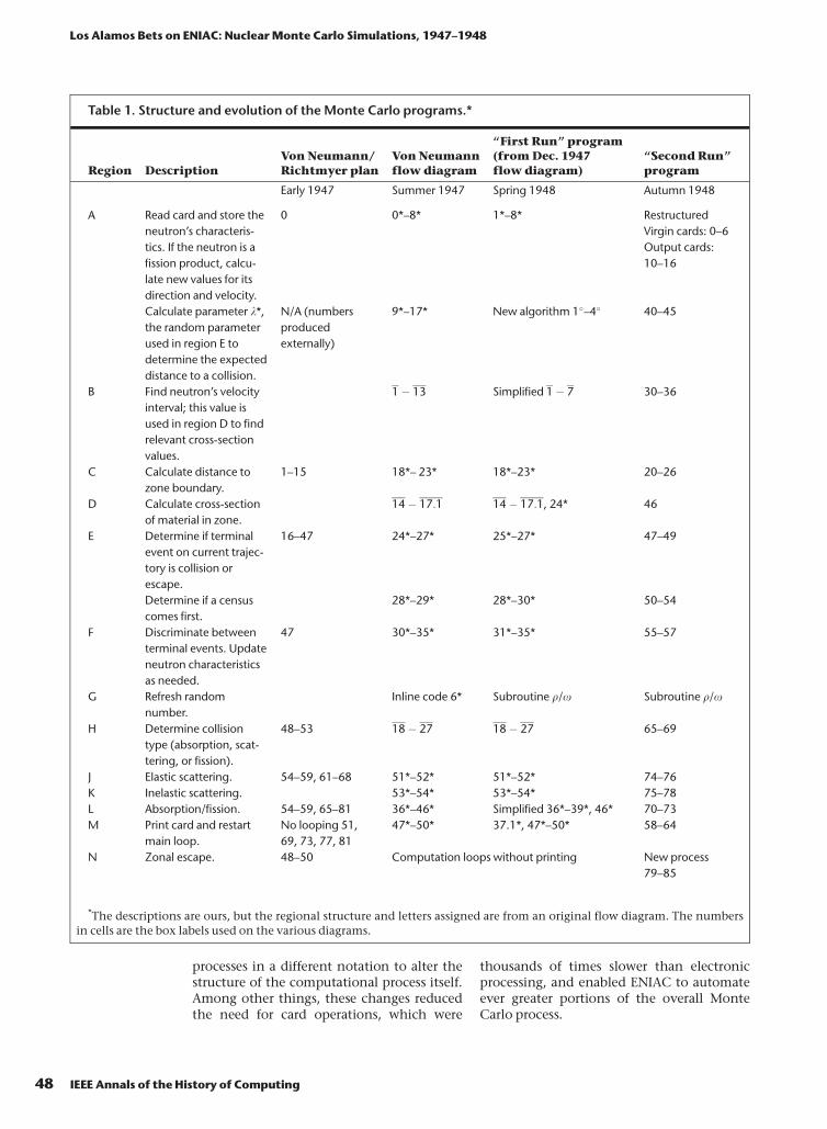
The timing estimates were later refined withthe aid of an overview flow diagram repre-senting just the structure of the computa-tion.38 This diagram was kept up to date asthe design evolved and changes were madeto the algorithms in various parts of the cal-culation, as Table 1 summarizes.

This was a complex program by the stand-ards of the day. The December 1947 flow dia-gram included 79 operation boxes, manyinvolving multiple computational steps (seeFigure 1).

The program was carefully structured in-to largely independent functional regions.Many of them are single-entrance, single-exitblocks. These regions first appeared in vonNeumann’s diagram, which was divided into10 spatially distinct subdiagrams linked byconnectors. Twelve regions were made ex-plicit and labeled in the subsequent overviewdiagram, and they are clearly visible in theDecember 1947 diagram, where many of theboundaries between the regions are markedby annotations in the form of “storage tables”noting the variables calculated in the preced-ing region and the accumulator assigned toeach.39

As Table 1 indicates, the changes in theevolution of the program can be tracked bythe rather confusing conventions used toassign numbers to the operation boxes in theflow diagram. The basic sequence of boxes 0*to 54* implemented the functionality ofthe original computing plan along with themodifications suggested by Los Alamos. Theswitch from ENIAC’s original programmingmethod to its new implementation of themodern code paradigm allowed for a signifi-cant expansion of the program’s scope andcomplexity. Thus, this original sequenceaccounted for little more than half of theeventual code. Changes made as develop-ment moved from the original plan to thefirst Monte Carlo code went far beyond elab-orating storage mechanics or expressing


processes in a different notation to alter thestructure of the computational process itself.Among other things, these changes reducedthe need for card operations, which were

thousands of times slower than electronicprocessing, and enabled ENIAC to automateever greater portions of the overall MonteCarlo process.

Table 1. Structure and evolution of the Monte Carlo programs.*

Region DescriptionVon Neumann/Richtmyer plan

Von Neumannflow diagram

“First Run” program(from Dec. 1947flow diagram)

“Second Run”program

Early 1947 Summer 1947 Spring 1948 Autumn 1948

A Read card and store the

neutron’s characteris-

tics. If the neutron is a

fission product, calcu-

late new values for its

direction and velocity.

0 0*–8* 1*–8* Restructured

Virgin cards: 0–6

Output cards:

10–16

Calculate parameter k*,

the random parameter

used in region E to

determine the expected

distance to a collision.

N/A (numbers

produced

externally)

9*–17* New algorithm 1�–4� 40–45

B Find neutron’s velocity

interval; this value is

used in region D to find

relevant cross-section

values.

1� 13 Simplified 1� 7 30–36

C Calculate distance to

zone boundary.

1–15 18*– 23* 18*–23* 20–26

D Calculate cross-section

of material in zone.

14� 17:1 14� 17:1, 24* 46

E Determine if terminal

event on current trajec-

tory is collision or

escape.

16–47 24*–27* 25*–27* 47–49

Determine if a census

comes first.

28*–29* 28*–30* 50–54

F Discriminate between

terminal events. Update

neutron characteristics

as needed.

47 30*–35* 31*–35* 55–57

G Refresh random

number.

Inline code 6* Subroutine q/x Subroutine q/x

H Determine collision

type (absorption, scat-

tering, or fission).

48–53 18� 27 18� 27 65–69

J Elastic scattering. 54–59, 61–68 51*–52* 51*–52* 74–76

K Inelastic scattering. 53*–54* 53*–54* 75–78

L Absorption/fission. 54–59, 65–81 36*–46* Simplified 36*–39*, 46* 70–73

M Print card and restart

main loop.

No looping 51,

69, 73, 77, 81

47*–50* 37.1*, 47*–50* 58–64

N Zonal escape. 48–50 Computation loops without printing New process

79–85

*The descriptions are ours, but the regional structure and letters assigned are from an original flow diagram. The numbersin cells are the box labels used on the various diagrams.



Change 1: Relaxation of NotationLooking closely at the succession of draftflow diagrams gives some insight into theexperience of using this technique to developan actual program. Von Neumann’s early dia-gram sticks closely to the notation publishedin the “Planning and Coding” reports: sym-bolic names are used for storage locations,and substitution and operation boxes areused in a systematic manner to keep mathe-matical notation separate from the handlingof storage. He extended the notation slightlyby including operations in the alternativeboxes and by using ad hoc notes within oper-ation and storage boxes to document theeffect of input and output operations.

The team seems to have found the com-plete methodology defined in the IAS re-ports to be excessively cumbersome, and byDecember, their use of the flow diagram nota-tion had visibly evolved (see Figure 2). Forexample, the symbolic labels for storage loca-tions were replaced by explicit references toENIAC’s accumulators. Decisions about datastorage had been taken, and there was evi-dently no perceived benefit in deferring theirdocumentation to a later stage in the process.The careful distinctions made in the reportsbetween the different types of boxes and theircontents are becoming increasingly blurred:the substitution boxes that are meant tocontrol loops have largely been replaced byoperation boxes, and storage updates thatofficially should be located in separate opera-tion boxes are appearing with increasing fre-quency in alternative boxes.

Change 2: A Subroutine to HandleRandom NumbersThe heart of a Monte Carlo simulation ischoosing between different possible outcomeson the basis of their probability. These choiceswere driven by random numbers, now re-quired in unprecedented numbers. In vonNeumann’s original plan for the computation,each card fed into ENIAC included the ran-dom numbers used to determine a neutron’sfate. Getting these numbers onto the cardswould have involved an additional process toproduce cards holding random numbers, fol-lowed by a merge process using conventionalpunched card machines to create a new cardholding both the existing data on a particularneutron (read from one card) and the randomnumbers (read from another).

As planning continued, von Neumannrealized that the ENIAC could itself producequasi-random numbers. In various letters, he

described a technique that involved squar-ing an eight- or 10-digit number, and thenextracting the middle digits to serve as thenext value.40 Thanks to the new programming

Figure 1. Detail from the December 1947 flow diagram. These largely

independent functional regions first appeared in John von Neumann’s

diagram, which was divided into 10 spatially distinct subdiagrams

linked by connectors. (Reproduced from the Library of Congress with

permission of Marina von Neumann Whitman. The full diagram,

together with other project materials, is available from www.

EniacInAction.com.)

Figure 2. The structure and mathematics of this part of the calculation

were almost unchanged between drafts, but in John von Neumann’s

early draft (white on black) the computation relies on symbolic storage

locations (such as B.4). The December 1947 version uses accumulator

numbers directly for storage (for example, 19). Note also the complex

expressions accommodated within individual flow diagram boxes, such

as 52*. (Reproduced from the Library of Congress with permission of

Marina von Neumann Whitman.)


mode, the logical complexity of a programwas limited only by the space available for itsinstructions on the function table. Thus,these numbers could be produced within theMonte Carlo program itself much more rap-idly than they could be read from punchedcards.

In the earlier draft flow diagram, a clusterof three boxes representing this process(without providing much detail on the algo-rithm to be used) was simply duplicated in-line at the four points in the computationwhere a new random number was needed.The December 1947 version placed a detailedtreatment of the process in a special box,entered from two separate places in the flowdiagram.41 The random digits it computedwere placed in one of the ENIAC’s accumula-tors. This exploited the newly developedconcept of a subroutine and demonstrated,apparently for the first time, the incorpora-tion of a subroutine call into the Goldstineand von Neumann flow diagram notation.42

Their “Planning and Coding” series had notso far dealt with subroutines (these would becovered in the final installment issued in1948). However, the April 1947 publicationdid introduce a “variable remote connection”

notation that diagrammed code in which thedestination of a jump was set dynamically. Inthe December 1947 flow diagram, a variableremote connection was used to return to themain sequence at the end of the subroutinebox (see Figure 3).

The invention of the “closed subroutine,”defined by Martin Campbell-Kelly as one that“appeared only once in a program and wascalled by a special transfer-of-control se-quence at each point in the programme whereit was needed,” is conventionally attributed toDavid Wheeler’s work with the EDSAC, whichbegan operation in 1949.43 This is distin-guished from the “open subroutine,” inwhich a block of code is duplicated as needed,a technique used on the Harvard Mark I someyears earlier. We believe that this ENIACMonte Carlo program was the first code with aclosed subroutine to be executed.44

Change 3: Lookup of Cross-section DataThe odds that a moving object crashes intoan obstacle during a particular time periodwill change with its velocity, as will the chan-ces of a destructive outcome. In nuclearphysics, the probability that a neutron willinteract with a nucleus to produce a particu-lar result, such as absorption, fission, or scat-tering, is referred to as a collision cross-section.This depends on both the velocity of the neu-tron and the nature of the material it is travel-ling through. Von Neumann’s original planrepresented the cross-sections as functions ofvelocity, and he noted that these functionscould be tabulated, interpolated, or approxi-mated using polynomials. By the time theearlier flow diagram was produced, he haddecided to use lookup tables. The range ofpossible neutron velocities was divided into10 intervals, giving 160 possible combina-tions of collision type, velocity interval, andmaterial. A representative cross-section func-tion value for each combination was storedin a matrix on the numeric function table,and his flow diagram incorporated a newsequence of boxes 1� 27 to handle thelookup procedure.45

A neutron’s velocity interval was found bysearching through a table of interval bounda-ries. This search was coded as a loop, provid-ing an early example of an iterative procedurewhose purpose was not simple calculation.Once the velocity interval had been located,the appropriate cross-section value couldeasily be retrieved from the function table bycalculating the address corresponding to thecurrent combination of parameters.

Figure 3. This detail from the December 1947 flow diagram shows both

the subroutine (far left) and one of the points from which it is called

(the connection q following box 32.1*). This box sets the value of the

variable remote connection x to x2 so that control will return to box 18

on completion. (Reproduced from the Library of Congress with

permission of Marina von Neumann Whitman.)



The design of the search went through anumber of revisions. The correct interval fora neutron was found by comparing its veloc-ity with the middle value in the table andthen performing a linear search through thetop or bottom half of the table, as appropri-ate. This strategy can be seen in the initialbranching in the diagrams shown in Figure 4,which in each case is followed by two simi-larly structured loops. Originally, the addressm of the current position in the table wasused to control the loop, and the number ofthe interval, k, was then calculated from thisin different ways, depending on how theloop had terminated (boxes 10� 13). Thiswas soon changed, however, so that the inter-val number itself was used to control theloop, leading to a significant simplification inthe expression of the termination conditions.These changes give a vivid impression of theteam gradually acquiring a feel for idiomatictechniques of efficient programming in themodern code paradigm.

The introduction of velocity intervals alsomade it possible to simulate fission more real-istically. In the initial plan the “daughter”neutrons produced by fission all had the

same velocity. After velocity intervals wereintroduced, a representative value known asthe “center of gravity” was stored for eachinterval. This allowed different velocities tobe easily generated for daughter neutrons byusing a digit from the current random num-ber to select a velocity interval.

Change 4: Census TimesThe biggest change in scope from the initialcomputing plan to the program initially exe-cuted was the transition from following anindividual neutron until it experienced itsnext “event” to managing a population ofneutrons over time. Translating the plan intoan ENIAC program made explicit, and parti-ally automated, the work needed to managemultiple neutrons over multiple cycles ofsimulation. Code implementing the steps de-fined in the original plan to process one neu-tron for one event was wrapped in severallevels of loops involving both automatic andmanual processing steps.

The program was organized around thenotion of “census times.” This idea was intro-duced by Richtmyer in his response to vonNeumann’s original computing plan, when

Figure 4. Three progressively more optimized versions of region B of the flow diagram, which finds a

neutron’s velocity interval. Image 1 is from von Neumann’s original flow diagram, and image 3 is from

the December 1947 diagram. Image 2 is an intermediate sketch.46 (Reproduced from the Library of

Congress with permission of Marina von Neumann Whitman.)


he observed that it would generate outputdecks in which cards held snapshots ofneutrons at widely different points in time.Richtmyer suggested as a “remedy for thisdifficulty” to

follow the chains for a definite time ratherthan for a definite number of cycles of opera-tion. After each cycle, all cards having t[ime]greater than some preassigned value would bediscarded, and the next cycle of calculationperformed with those remaining. This wouldbe repeated until the number of cards in thedeck diminishes to zero.47

These preassigned values were dubbed“census times.” A statistically valid picture ofthe overall neutron population at these pointswould then be produced, just as governmentsmake measurements of the characteristics oftheir national populations at certain periodicdates. The census concept was widely adoptedfor Monte Carlo simulations.48

Change 5: Simulating Multiple Events Per CycleAccording to the original computing plan,each cycle of computation would track theprogress of a neutron only as far as its nextevent (scattering, zonal escape, total escape,absorption, or fission). One or more newcards representing the consequences of theevent would then be produced. The addi-tional logical complexity afforded by the newprogramming mode made it possible forENIAC to simulate more than one event in aneutron’s career before printing a new cardfor it. If a neutron was scattered or movedinto a new zone but had not yet reached thecensus time, the program branched back toan earlier region to follow its progress furtherrather than producing an output card imme-diately. This increased the complexity of theprogram but reduced the amount of manualcard processing required.

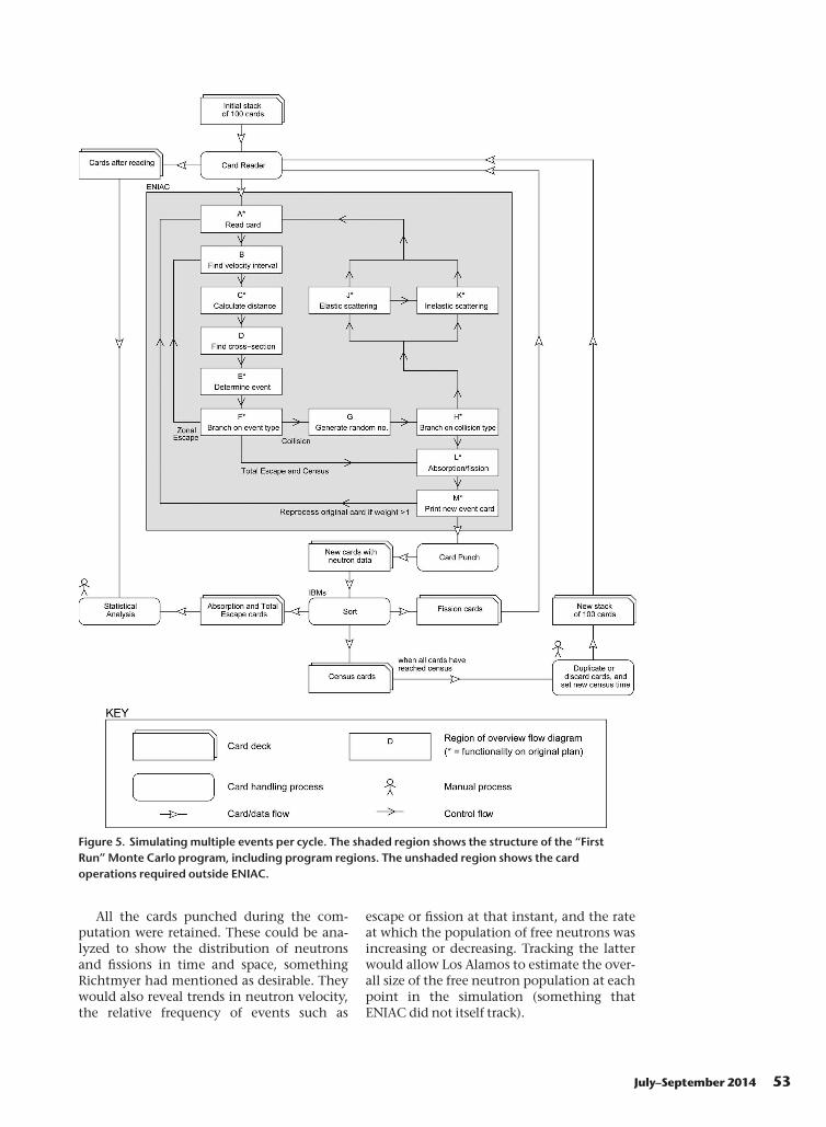
Figure 5 gives an overview of how all thisworked in practice. The initial stack of neu-tron cards was read one at a time from theinput hopper. After reading each card, ENIACpunched one or more output cards. If a neu-tron reached the current census time withoutincident, it was followed no further for themoment and ENIAC output a “census” cardwith its updated information. If a neutron wasabsorbed or experienced total escape, then itscareer as a free neutron within the simulationwas over, but a card identifying the natureof the terminal event was nevertheless out-put for analytical processes. Likewise, when

a neutron triggered fission, a terminal cardfor that neutron was produced specifyingthat fission had taken place, including a“weight” field to indicate the number ofdaughter neutrons set free.

ENIAC’s operators would then use a suit-ably configured sorting machine to separatethe output deck into three trays. One trayaccumulated cards representing neutronsthat did not need to be processed againbecause they had terminated their simulatedcareer after escaping or being absorbed.Another tray accumulated census cards repre-senting neutrons that had reached the cur-rent census time without incident.

The third tray held the cards representingsimulated fission events. Because these fis-sions had taken place before the end of thecurrent census period, the cards were carriedover to ENIAC’s input hopper for furtherprocessing.49 The data on this card was readonce, but ENIAC processed it repeatedly tosimulate each daughter neutron generated bythe fission. The careers of these daughter neu-trons were followed as normal, with one cardbeing punched for each when a terminalevent was reached. These output cards weresorted again, in case any further fissions hadoccurred, and the process repeated untilENIAC’s output deck included no fissioncards, indicating that each neutron had beenfollowed up to the census time.

At this point, the target census time couldbe incremented and the simulation couldmove on to the next census period. The pileof census cards, representing neutrons thatwere still active at the end of the previousperiod, provided the new input deck. How-ever, it needed additional manual processingbefore use. The team had decided to starteach census period with the same number ofneutrons, even though the number of neu-trons careening around inside a bomb tendsto rise or fall precipitously after its detonatoris triggered. A larger neutron sample popula-tion increased statistical confidence in theresults of the simulation but increased thetime, work, and pile of punched cards neededto run it. A smaller neutron sample popula-tion could be processed more quickly but itsbehavior would be less likely to track thelarger system being simulated. Thus, allowingthe neutron sample size to grow or shrink inproportion to the simulated populationwould sacrifice either accuracy or practicality.Cards from the deck were therefore manuallyduplicated or discarded to create a new inputdeck of 100 cards.



All the cards punched during the com-putation were retained. These could be ana-lyzed to show the distribution of neutronsand fissions in time and space, somethingRichtmyer had mentioned as desirable. Theywould also reveal trends in neutron velocity,the relative frequency of events such as

escape or fission at that instant, and the rateat which the population of free neutrons wasincreasing or decreasing. Tracking the latterwould allow Los Alamos to estimate the over-all size of the free neutron population at eachpoint in the simulation (something thatENIAC did not itself track).

Figure 5. Simulating multiple events per cycle. The shaded region shows the structure of the “First

Run” Monte Carlo program, including program regions. The unshaded region shows the card

operations required outside ENIAC.


Making the First Run, April–May 1948The three main sets of Monte Carlo chainreactions carried out for Los Alamos in 1948and 1949 were referred to by the von Neu-manns as the “first run,” “second run,” and“third run.” Within each run a differentevolution of the program code was used toinvestigate a number of “problems,” eachsimulating a different physical configuration.The term “run” may echo the idea, later ubiq-uitous, of “running” a program or may referinstead to the physical movement of peopleand materials to Aberdeen and back—in thesense of a “bombing run” or “school run.”The term “expedition” was also used by Johnvon Neumann to refer to these trips and tolater trips made to Aberdeen to experimentwith numerical weather predictions.50 It is astriking term, capturing a world in whichcomputers were scarce and exotic things byevoking the scientific tradition of mountinglong, arduous, and painstakingly plannedfield expeditions to observe eclipses, uncoverburied cities, or explore the polar regions.Explorers returned with knowledge thatcould never be obtained at home. UsingENIAC was an adventure, a journey to anunfamiliar place, and often something of anordeal.

Anne Fitzpatrick, who wrote with accessto internal Los Alamos progress reports andother classified documents, concluded thatall ENIAC Monte Carlo work done for LosAlamos in 1948 and 1949 was focused on fis-sion weapons, rather than relating directly tothe fusion-powered hydrogen bomb. The ini-tial set of seven calculations in spring 1948were “primarily for the purpose of checkingtechniques, and according to Metropolis, didnot attempt to solve any type of weaponsproblem.” It is, however, clear that Los Ala-mos viewed the work on ENIAC as crucial toits own progress with new weapons designs.Fitzpatrick continues,

Throughout March and April Carson Mark[director of the lab’s Theoretical Division] com-plained in his monthly reports about thedelays encumbered (sic.) by the fissionprogram because of the slow pace of theENIAC’s conversion and “mechanical con-dition.” The whole point of having fissionproblems run on ENIAC in the first place, Marknoted, was to speed up T Division’s work by“mechanization” of calculations.51

Even a man as well connected as John vonNeumann could not simply show up at theBallistic Research Laboratory in Aberdeen

and ask his friends for the keys to ENIAC.There were bureaucratic niceties to followand a chain of command to respect. On 6February 1948, he wrote to Norris Bradbury,director of Los Alamos, asking him to make aformal request for time on the ENIAC. Politi-cal as ever, von Neumann reminded Bradburyto “mention in your letter how much youappreciate all the courtesies that have beenextended to your staff by the BRL and howextremely important the ENIAC is to yourwork, etc. This will greatly help ColonelSimon politically and will also be good for ourfuture relations with the BRL.”52

The terms had already been worked outinformally with Simon and his subordinates,with delays imposed by the arrival of ceilingcontractors, testing, and the delayed installa-tion of new hardware.53 Bradbury sent thenecessary official request, flattery included,to the Office of Chief of Ordnance. On 13March 1948, von Neumann wrote to CarsonMark, leader of the Theoretical Division atLos Alamos, that “The Monte Carlo problemis set up and ready to go.”54

The von Neumanns visited Aberdeen on 8April 1948, and Klara remained behind forthe next month to work with Metropolis,who had by then completed initial reconfigu-ration of ENIAC to support the modern codeparadigm. The first successful “productionrun” made on Monte Carlo took place on 17April 1948. However, the machine was stillplagued by “troubles” and the calculation didnot begin in earnest until 28 April.55 Progressseems to have been slowed far more by hard-ware glitches than program bugs, which isinteresting given that nobody had previouslydebugged a program written in the moderncode paradigm. This is a tribute to the carewith which the program had been planned,the depth of thought the Princeton grouphad given to the new programming style,and perhaps also to ENIAC’s relative friendli-ness to debugging.

We have not located the program code forthe first run. However, triangulating fromseveral sources gives a reliable sense of howthis first Monte Carlo worked. First, we havethe series of flow diagrams discussed previ-ously. Second, we have the revised programcode used for the second run in late 1948.Third, we have a lengthy archival document,“Actual Running of the Monte Carlo Prob-lems on the ENIAC,” which describes theprogramming techniques used in bothversions. This explicitly highlights changesmade between the two runs. Fourth, the draft



flow diagrams for the second run are in manyregions identical to the first run diagram.Finally, archival materials for the first rundocument the allocation of data to theENIAC’s accumulators, the layout of constantdata on the third function table, the card for-mat used, and the associated use of the con-stant transmitter.56

The calculations performed during thefirst run simulated seven different situations,each represented by changing some of thedata stored on the third function table. AsRichtmyer wrote,

Certain experimentally determined nucleardata are obviously needed. One must know theso-called macroscopic cross-sections, that is,the probabilities, per unit distance travelled, ofthe various processes (absorption, elastic scat-tering, inelastic scattering) in each medium,as a function of the neutron’s velocity. Forscattering, one must know the angular distri-bution, that is, the relative probabilities of vari-ous angles of scattering; for inelastic scatteringone must also know the energy distribution ofthe scattered neutrons; and, for fission, onemust know the average number and energydistribution of the emitted neutrons.57

This data was the most militarily sensitivepart of the entire operation. Documentsretained in the archives record in triplicatethe receipt of classified material by Klara vonNeumann on various occasions, sometimes(as with “cross section data” on 16 January1947) from her husband.58

Our companion article “Engineering ‘TheMiracle of ENIAC’”3 discusses several draftinstruction sets created for ENIAC during theplanning process. For the first run program,ENIAC was set up to implement a codeproviding 79 instructions.59 This would nothave required major changes to draft pro-grams targeting the “60 order code.” Beyondupdating the numerical codes correspondingto the instruction mnemonics, a simple mat-ter of substitution, the main challenge wouldhave been restructuring shift instructions asthese were handled quite differently in thenew instruction set.

By 10 May 1948 it was all over. John vonNeumann wrote on 11 May to Ulam that“ENIAC ran for 10 days. It was producing50% of these 10x16 hours, this includes twoSundays and all troubles…. It did 160 cycles(’censuses,’ 100 input cards each) on 7 prob-lems. All interesting ones are stationary at theend of this period. The results are very prom-ising and the method is clearly a 100%

success.”60 Three days later, he added that“There is now a total output of over 20,000cards. We have started to analyze them, but… it will take some doing to interpret it.”61

Klara von Neumann documented thetechniques used in a manuscript crypticallyheaded “III: Actual Technique—The Use ofthe ENIAC.”62 This began with a discussionof the conversion of ENIAC to support thenew code paradigm, documented the dataformat used on the punched cards, and out-lined in reasonable detail the overall struc-ture of the computation and the operationsperformed at each stage.

Second Run, October–November 1948Klara von Neumann returned to Aberdeen on18 October 1948 to perform a second run ofMonte Carlo calculations and was joined byMetropolis two days later. Production workbegan on 22 October. On 4 November, Johnvon Neumann wrote to Ulam that “[t]hingsat Aberdeen have gone very well. The presentsegment of the Monte Carlo program is likelyto be completed at the end of this week orearly next week.”63 According to Fitzpatrick,this second series of problems “constitutedactual weapons calculations” including “aninvestigation of the alpha for UH3, a‘hydride’ core implosion configuration” and“a supercritical configuration known as theZebra.”64

Changes between the first and second ver-sions of the Monte Carlo program weredescribed in some detail in the report “ActualRunning of the Monte Carlo Problems on theENIAC.” An expanded and updated versionof the earlier “Actual Technique” report, thiswas written by Klara von Neumann andedited in collaboration with Metropolis andJohn von Neumann during September 1949.It contains a detailed description of the com-putations, highlighting the changes in theflow diagram, program code, and manualprocedures between the two versions.65

The physical model used and the cal-culations performed to follow the paths ofindividual neutrons were little changed.Modifications were made to representationsof the zones of different materials and of thezonal escape of neutrons. Most changes wereoperational optimizations. For example,some early sections of the program were reor-dered to marginally increase overall effi-ciency, and collision cross-section ratios wereprecomputed and stored on the functiontable to avoid recalculating them whenneeded.


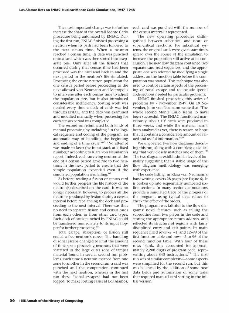
The most important change was to furtherincrease the share of the overall Monte Carloprocedure being automated by ENIAC. Dur-ing the first run, ENIAC finished processing aneutron when its path had been followed tothe next census time. When a neutronreached a census time, its data was punchedonto a card, which was then sorted into a sep-arate pile. Only after all the fissions thatoccurred during that census time had beenprocessed was the card read back in and thenext period in the neutron’s life simulated.Processing the entire neutron population forone census period before proceeding to thenext allowed von Neumann and Metropolisto intervene after each census time to adjustthe population size, but it also introducedconsiderable inefficiency. Sorting work wasneeded every time a deck of cards was fedthrough ENIAC, and the deck was examinedand modified manually when processing foreach census period was completed.

The second run eliminated both kinds ofmanual processing by including “in the logi-cal sequence and coding of the program, anautomatic way of handling the beginningand ending of a time cycle.”66 “No attemptwas made to keep the input stack at a fixednumber,” according to Klara von Neumann’sreport. Indeed, each surviving neutron at theend of a census period gave rise to two neu-trons in the next period to ensure that thesample population expanded even if thesimulated population was falling.67

As before, reading a fission or census cardwould further progress the life history of theneutron(s) described on the card. It was nolonger necessary, however, to process all theneutrons produced by fission during a censusinterval before rebalancing the deck and pro-ceeding to the next interval. There was thusno need to separate fission and census cardsfrom each other, or from other card types.Each deck of cards punched by ENIAC couldbe transferred immediately to its input hop-per for further processing.68

Total escape, absorption, or fission stillended a free neutron’s career. The handlingof zonal escape changed to limit the amountof time spent processing neutrons that werescattered in the large outer zone of tampermaterial found in several second run prob-lems. Each time a neutron escaped from onezone to another in the second run, a card waspunched and the computation continuedwith the next neutron, whereas in the firstrun these “zonal escapes” had not beenlogged. To make sorting easier at Los Alamos,

each card was punched with the number ofthe census interval it represented.

The new operating procedures distin-guished between subcritical and near- orsuper-critical reactions. For subcritical sys-tems, the original cards were given start timesspread over the course of the simulation toincrease the proportion still active at its con-clusion. The new flow diagram contained twoseparate card read sequences, and the appro-priate one was selected by modifying a singleaddress on the function table before the com-putation was started. This technique was alsoused to control certain aspects of the process-ing of zonal escape and to include specialcode sections needed for particular problems.

ENIAC finished processing this series ofproblems by 7 November 1949. On 18 No-vember, John von Neumann wrote that “Thewhole second Monte Carlo seems to havebeen successful. The ENIAC functioned mar-velously. About 105 cards were produced inthree weeks, and while the material hasn’tbeen analyzed as yet, there is reason to hopethat it contains a considerable amount of val-ued and useful information.”69

We uncovered two flow diagrams describ-ing this run, along with a complete code list-ing that very closely matches one of them.70

The two diagrams exhibit similar levels of for-mality suggesting that a stable usage of theflow diagram methodology was emergingwith experience.

The code listing, in Klara von Neumann’shandwriting, covers 28 pages (see Figure 6). Itis broken up into sequentially numbered six-line sections. In many sections annotationsprovide a simulated trace of the progress ofthe program, using typical data values tocheck the effect of the orders.

The program was faithful to the flow dia-grams’ novel features, such as calling thesubroutine from two places in the code andstoring the appropriate return address, andreflected its structure of regions with fairlydisciplined entry and exit points. Its mainsequence filled rows –2, –1, and 12–99 of thefirst function table and rows –2 to 96 of thesecond function table. With four of theserows blank, this accounted for approxi-mately 2,208 digits of program code, repre-senting about 840 instructions.71 The firstrun was of similar complexity—some aspectswere simplified for the second run, but thiswas balanced by the addition of some newdata fields and automation of some tasksthat required manual card sorting in the ini-tial version.



The code for the second run included anumber of variant paths and sections andcould be configured for a specific problemby manually setting a handful of transferaddresses within instructions on the functiontables before execution was started. The mostsignificant of these is a section of code dealingwith the elastic scattering of neutrons in “lightmaterials.” This reflected interest at Los Ala-mos in the use of uranium hydride cores. Thehydrogen separates from the uranium, actingas a moderator to slow neutrons and reducethe critical mass of uranium needed to build aweapon. Edward Teller believed, wrongly as itturned out, that the inevitable reduction inexplosive yield would be more than offset byof the opportunity to build more bombs fromscarce weapons-grade uranium.72

Klara von Neumann left for Los Alamosaround 1 December, presumably to help inter-pret the second run results and to lay thegroundwork for future calculations. A letterfrom her husband, who arrived some weekslater, expressed “dense confusion” after whatseemed to be some kind of argument triggeredby a crisis of confidence on her part as she pre-pared to provide “proof of [her] intellectualindependence” via this solo trip.73 Even some-one blessed with ample self-confidence androbust mental health would feel somewhatdaunted at the prospect of defending one’smathematical technique to Ulam, Teller, andEnrico Fermi (the latter already a Nobel Prizewinner). On 13 December, John wrote to herat Los Alamos to admit himself “scared out ofmy wits” after finding her “catastrophicallydepressed” during a phone call and worryingthat the stress would leave her ruined“physically and emotionally.” Seeking inde-pendence within the shadow of John vonNeumann only added to the challenges facingKlara, despite his fervent attempts to allay herworries about her loss of youth (“your prob-lems and dispositions are perennial, and age isthe least of your troubles”), intelligence (“abright girl”) and flawed character (“and a verynice one”).74

Her worries could only have been com-pounded when an error was discovered in thehydride calculations. Ulam wrote to John vonNeumann on 7 February that “It seems thatour electronic computation is wrong in theProblem No. 4—Nick found out which it was.The problem has to be repeated.”75 CarsonMark complained in his regular Theory Divi-sion progress report that it was “evident thatthe ENIAC has not advanced beyond an exper-imental stage in doing serious computation

for this project.”76 These gripes did not deterfurther use of ENIAC or slow Monte Carlo’srapid enshrinement as an indispensable toolfor nuclear science. ENIAC and Klara von Neu-mann hosted at least three further MonteCarlo expeditions by the staff of Los Alamosand Argonne labs during 1949 and 1950 beforemore powerful computers became availablefor their use.

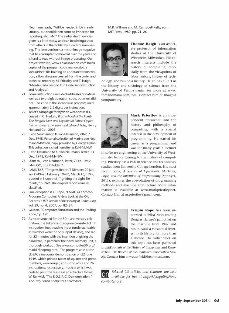
ConclusionsJohn von Neumann’s contribution to thedevelopment of modern computing is wellknown, and the roles of some of his collabora-tors such as Herman Goldstine and ArthurBurks are also well documented. Our investi-gation has shed new light on the importance

Figure 6. Detail from page 7 of the second run

program code, showing 13 of the 840

instructions in the program. Numbers 65–68

show positions on the function tables, and

annotations in the left margin refer back to the

corresponding boxes on the flow diagram. Each

row gives the two decimal digits entered on the

function table, and when those numbers code an

operation rather than a data field, the

corresponding mnemonic such as 3l or N3D8.

Some corrections have been made in red pencil,

and blocks 65 and 66 of code have been erased

and substituted for each other. (Reproduced

from the Library of Congress with permission of

Marina von Neumann Whitman.)


of work done by some of his other collabora-tors, most notably his wife Klara. Her centralcontribution to the Monte Carlo workhas, with the exception of previously citedcomments by Nick Metropolis and recentcoverage by George Dyson, barely been men-tioned.77 The story told here fits, in its broadoutline, with Galison’s famous depiction ofthe first Monte Carlo simulations as a tradingzone, yet stepping down from his lofty perchto look more closely at the details of the com-putations deepens our understanding of whatis being traded and by whom.

According to Galison, Monte Carlo ledphysics to a “netherland that was at oncenowhere and everywhere.”78 This descriptionof its intellectual legacy also describes itsunconventional social structure, creatingopportunities in the shadows. The practice ofMonte Carlo engaged not only the great menpopulating his story, who were diverse intheir disciplinary backgrounds, but a broadercast of characters. In particular, Klara vonNeumann, mentioned by Galison only asone of a list of early female computer pro-grammers, emerges as a surprisingly centralparticipant in these exchanges. Entering thetrading zone with no scientific credentials,carrying little more than her natural talentand some social capital borrowed from herhusband, she was soon running a successfulstall of her own.

The ENIAC Monte Carlo simulations exe-cuted from spring 1948 onward stand outamong the programs executed during the1940s for their complexity and the fidelity oftheir diagramming and coding style to theideas of John von Neumann and his circle ofcollaborators. Our analysis illuminates theevolution of the program over a two-yearperiod from an initial computing plan,through a series of flow diagrams to an initialENIAC program and onward through a majorcycle of revision and improvement. Thisgives a uniquely detailed and richly substan-tiated look at a landmark program.

The program challenges some generaliza-tions about scientific computing. We tend tothink of the speed and practical scope of earlyscientific computer problems as governedlargely by computation speed and memoryrequirements with minimal requirements forinput and modest output needs, in contrastwith administrative data processing jobswhere throughout depended on the speed atwhich data could be pushed in and out of themachine from card or tape units. ENIAC’soriginal task of calculating trajectory tables

certainly fits this model, as do the celebrated“first programs” run on the Manchester Babyand EDSAC (both of which performed longseries of calculations with no data input anda tiny output consisting of solutions).79 Incontrast, the first program run on ENIACafter its conversion to the new code paradigmwas a complex simulation system that mighttake days to complete its tasks, dependingprimarily on the speed at which data couldbe fed through the machine.

The program included a number of key fea-tures of the modern code paradigm. It wascomposed of instructions written using asmall number of operation codes, some ofwhich were followed by additional argu-ments. Conditional and unconditional jumpswere used to transfer control between differ-ent parts of the program. Instructions anddata shared a single address space, and loopswere combined with index variables to iteratethrough values stored in tables. A subroutinewas called from more than one point in theprogram, with the return address stored andused to jump back to the appropriate place oncompletion. Whereas earlier programs, suchas those run on the Harvard Mark I, were writ-ten as a series of instructions and codednumerically, this was the first program everexecuted to incorporate these other key fea-tures of the modern code paradigm.

Acknowledgments

This project was generously funded by Mrs.

L.D. Rope’s Second Charitable Settlement.

Thanks to archivists Susan Dayall at Hamp-

shire College, Lynn Catanese at the Hagley

Museum and Library, Susan Hoffman at the

Charles Babbage Institute, Valerie-Ann Lutz

and the other archival staff at the American

Philosophical Society, and the staff of the

Library of Congress Manuscripts Reading

Room. Nate Wiewora, Alan Olley, and Peter

Sachs Collopy provided us with copies of

documents. George Dyson and Marina von

Neumann Whitman both shared unpub-

lished material with us from the latter’s per-

sonal collection of papers concerning Klara

von Neumann. Susan Abbey provided hand-

writing analysis services to clarify the

authorship of numerous documents. Anne

Fitzpatrick, Steve Aftergood, Robert Seidel, J.

Arthur Freed, and Alan B. Carr all did what

they could to help us navigate the maze of

restrictions surrounding access to historical



materials from Los Alamos. William Aspray,

Jeff Yost, Atsushi Akera, Paul Ceruzzi, and

Martin Campbell-Kelly kindly answered our

questions on specific topics and shared their

perspectives on computing in the 1940s. We

also benefitted from suggestions made by

the Annals reviewers and by those who dis-

cussed the draft at the informal Workshop

on Early Programming Practice, organized

by Gerard Alberts and Liesbeth De Mol.

References and Notes

1. J. von Neumann, “First Draft of a Report on the

EDVAC,” IEEE Annals of the History of Computing,

vol. 15, no. 4, 1993, pp. 27–75.

2. T. Haigh, M. Priestley, and C. Rope,

“Reconsidering the Stored Program Concept,”

IEEE Annals of the History of Computing, vol. 36,

no. 1, 2014, pp. 4–17.

3. T. Haigh, M. Priestley, and C. Rope,

“Engineering ‘The Miracle of the ENIAC’: Imple-

menting the Modern Code Paradigm,” IEEE

Annals of the History of Computing, vol. 36, no. 2,

2014, pp. 41–59.

4. An overview of perspectives on the history of

software toward the beginning of this period is

given in U. Hashagen, R. Keil-Slawik, and

A.L. Norberg, eds., Mapping the History of

Computing: Software Issues, Springer-Verlag,

2002.

5. Changes in the focus of software history over

time are explored in M. Campbell-Kelly, “The

History of the History of Software,” IEEE Annals

of the History of Computing, vol. 29, no. 4, 2007,

pp. 40–51.Recent contributions include M.

Campbell-Kelly, From Airline Reservations to Sonic

the Hedgehog: A History of the Software Industry,

MIT Press, 2003; T. Haigh, “How Data Got Its

Base: Information Storage Software in the 1950s

and 1960s,” IEEE Annals of the History of Comput-

ing, vol. 31, no. 4, 2009, pp. 6–25; M. Priestley,

A Science of Operations: Machines, Logic, and the

Invention of Programming, Springer, 2011.Our

specific topic, the programming of ENIAC, has

recently been explored in B.J. Shelburne, “The

ENIAC’s 1949 Determination of p,” IEEE Annals

of the History of Computing, vol. 34, no. 3, 2012,

pp. 44–54; and M. Bullynck and L. De Mol,

“Setting-Up Early Computer Programs: D.H.

Lehmer’s ENIAC Computation,” Archive for

Mathematical Logic, vol. 49, no. 2, 2010,

pp. 123–146.

6. See, for example, the perspectives gathered in

N. Oudshoorn and T. Pinch, eds., How Users

Matter: The Co-Construction of Users and Technol-

ogy, MIT Press, 2003.

7. P. Galison, “Computer Simulation and the Trad-

ing Zone,” The Disunity of Science: Boundaries,

Contexts, and Power, P. Galison and D.J. Stump,

eds., Stanford Univ. Press, 1996, p. 119.

8. Galison, “Computer Simulation and the Trading

Zone,” p. 120.

9. M.S. Mahoney, “Software as Science—Science

as Software,” Mapping the History of Comput-

ing: Software Issues, U. Hashagen, R. Keil-Sla-

wik, and A.L. Norberg, eds., Springer-Verlag,

2002, pp. 25–48. U. Hashagen, “The Computa-

tion of Nature, Or: Does the Computer Drive

Science and Technology?” The Nature of Com-

putation. Logic, Algorithms, Applications, P.

Bonizzoni, V. Brattka, and B. L€owe, eds., LNCS

7921, Springer-Verlag, 2013, pp. 263–270.

The philosophical status of early Monte Carlo

simulation was recently explored in a PhD the-

sis: I. Record, Knowing Instruments: Design, Reli-

ability, and Scientific Practice, History and

Philosophy of Science and Technology, Univ. of

Toronto, 2012.

10. The jump takes place at the bottom of page 130.

Pages 130–135 then discuss the application of

Monte Carlo methods to the Super, including

ENIAC calculations performed in 1950.

11. A. Fitzpatrick, “Igniting the Light Elements: The

Los Alamos Thermonuclear Weapon Project,

1942–1952 (LA-13577-T),” Los Alamos Nat’l

Lab., 1999.

12. D. MacKenzie, “The Influence of Los Alamos and

Livermore National Laboratories on the Devel-

opment of Supercomputing,” IEEE Annals of the

History of Computing, vol. 13, no. 2, 1991,

pp. 179–201.

13. W. Aspray, John von Neumann and the Origins of

Modern Computing, MIT Press, 1990.

14. The series of 1947–1948 reports on “Planning and

Coding Problems for an Electronic Computer” are

reproduced in W. Aspray and A.W. Burks, Papers of

John von Neumann on Computing and Computer

Theory, MIT Press, 1987, pp. 151–306.

15. S.M. Ulam, Adventures of a Mathematician,

Scribner, 1976, p. 148.

16. Fitzpatrick, “Igniting the Light Elements,”

p. 269.

17. Ulam, Adventures of a Mathematician,

pp. 196–201. Another first-hand account is

given in N. Metropolis, “The Beginning of the

Monte Carlo Method,” special issue, Los Alamos

Science, 1987. Several secondary treatments are

cited in subsequent notes.

18. Aspray, John von Neumann and the Origins of

Modern Computing, pp. 111, 288, footnote 50.

This public mention of Monte Carlo seems to

precede the well-known paper by von Neumann

and Ulam presented in September 1947 and

published as S.M. Ulam and J. Von Neumann,


“On Combination of Stochastic and Determinis-

tic Processes: Preliminary Report,” Bull. of the

Am. Mathematical Soc., vol. 53, no. 11, 1947,

p. 1120.

19. C.C. Hurd, “A Note on Early Monte Carlo

Computations and Scientific Meetings,”

Annals of the History of Computing, vol. 7, no.

2, 1985, pp. 141–155. The report repro-

duced there is the source for much subse-

quent discussion of the planned

computation, including Galison, “Computer

Simulation and the Trading Zone,”

pp. 129–130, and Record, Knowing Instru-

ments, pp. 137–141.

20. Richtmyer’s reply (also reprinted by Hurd in

his 1995 article) points out that the “slower-

down material” could be omitted for “systems

of interest to us [at Los Alamos]” (that is,

bombs). This suggestion was followed in the

first version of the program, although the

layer was eventually reintroduced to allow

simulation of bombs with uranium hydride

cores.

21. Von Neumann also proposed recording the cur-

rent zone number to save having to calculate

this based on the neutron’s position.

22. R.D. Richtmyer, “Monte Carlo Methods: Talk

Given at the American Mathematical Society, April

24, 1959,” p. 3. Stanislaw M. Ulam Papers, Am.

Philosophical Soc., series 15. (Further citations to

this collection are abbreviated SMU-APS.)

23. Hurd, “A Note on Early Monte Carlo

Computations and Scientific Meetings,”

p. 149.

24. These limitations are discussed further in

T. Haigh, M. Priestley, and C. Rope,

“Engineering ‘The Miracle of the ENIAC,’” p. 43.

25. Hurd, “A Note on Early Monte Carlo Computa-

tions and Scientific Meetings,” p. 152.

26. G. Dyson, Turing’s Cathedral: The Origins

of the Digital Universe, Pantheon Books, 2012,

p. 210.

27. J. von Neumann to Ulam, letter, 27 Mar.

1947, SMU-APS, series 1, John von Neumann

folder 2.

28. “I am hoping to hear very soon from the

‘Princeton Annex’ some word of the first

Monte Carlo.” C. Mark to J. von Neumann,

letter, 7 Mar. 1948, Papers of John von Neu-

mann, Manuscripts Division, US Library of

Congress, box 5, folder 13. (This collection is

cited hereafter as JvN-LOC).

29. Dyson, Turing’s Cathedral, pp. 175–189, focuses

on Klara von Neumann, as does M.v.N. Whitman,

The Martian’s Daughter: A Memoir, Univ. of

Michigan Press, 2012, pp. 22–23, 38–39, 48–54.

30. A letter dated 28 Aug. 1947 from A.W. Kelley to

Richtmyer confirms that the “necessary

approvals have been obtained” for her employ-

ment by Los Alamos. JvN-LOC box 19, folder 7.

However, her informal involvement seems to

have preceded this.

31. K. von Neumann, “Grasshopper in the Very Tall

Grass,” memoir (n.d.), Papers of Marina von

Neumann Whitman, 1946–2013, Schlesinger

Library, Radcliffe Inst. for Advanced Study, Har-

vard University. Transcription by M. von Neu-

mann Whitman.

32. Dyson, Turing’s Cathedral, p. 188.

33. These quotations are taken from Klara von Neu-

mann’s “Grasshopper in Very Tall Grass.”.

34. W. Aspray and A. Bucks, “Computer Program-

ming and Flow Diagrams: Introduction,” Papers

of John von Neumann on Computing and Com-

puter Theory, W. Aspray and A. Bucks, ed., MIT

Press, 1987, pp. 145–150.

35. The best developed version of the first run

flow diagram measured approximately 24

inches by 18 inches and is neatly written in

the hand of Adele Goldstine with the head-

ing “MONTE CARLO Flow Diagram 12/9/

47,” JvN-LOC, box 11, folder 7. (There are

two copies, one a negative.) A copy with

two later handwritten annotations is in the

Herman H. Goldstine Collection, 1941–1971

Archives, Hampshire College (hereafter cited

as HHG-HCA). This diagram is available

online from our project website www.EniacI-

nAction.com as is a technical report by

M. Priestley and T. Haigh, “Monte Carlo

Computation Analysis,” charting in more

detail the evolution of planning for the

computation.

36. Ten manuscript pages numbered I, II.a–II.g,

III, and IV, in JvN-LOC, box 11, folder 8. An

undated manuscript page on squared paper

in JvN-LOC box 11, folder 8, contains a plan

of ENIAC’s three function tables, labeled “FT

I,” “FT II,” and “FT III,” and shows that all

three tables could be used for the storage of

program instructions or numeric data. Com-

mon practice, followed in the Monte Carlo

programs, was to use two tables to store the

program code and the third, referred to as

the “numeric function table,” to hold data

describing a particular physical situation. This

strategy preserved the separation of the

setup of the Monte Carlo procedure itself

from what von Neumann referred to in his

original letter to Richtmyer as “numerical

constants” describing a particular “criticality

problem.” (Hurd, “A Note on Early Monte

Carlo Computations and Scientific Meetings,”

p. 149).

37. Undated manuscript page headed “Refresh Ran-

dom No.,” JvN-LOC, box 11, folder 8. J. von



Neumann was working personally on the meth-

ods for the generation of random numbers, so

this might well have been written before or sep-

arately from the rest of the program.

38. Seven undated manuscript pages numbered 0

to 6 and a single page headed “Shifts” in JvN-

LOC, box 11, folder 8. The structure of the

overview flow diagram on page 0 is reproduced

in the shaded area of Figure 5. Additional dia-

grams on pages 1–3 represented the operation

boxes and the connections between them in

each of the 12 regions. Pages 4–6 contained

detailed timing estimates for each box and

region.

39. Three storage tables can be seen in Figure 1, one

attached by a dashed line to the line between

boxes 1* and 1.2* and e.g. one to the right of

box 7*.

40. Von Neumann talks about the “square and take

the middle digits” approach to generating pseu-

dorandom numbers, and testing the resulting

distribution, in letters to A.S. Householder (3

Feb. 1948) and C.C. Hurd (3 Dec. 1948), J. von

Neumann, Selected Letters, M. R�edei, ed., Am.

Mathematical Soc., 2005, pp. 141–142,

144–145.

41. This was another minor optimization: two of the

four points at which new numbers had been

generated were, by late 1947, modified to make

use instead of particular digits within the num-

ber already generated.

42. The idea of a subroutine was familiar within the

ENIAC team as early as 1945: “It is possible to

have the main routine divided into sub-routines,

in which case one stepper is used to feed another

stepper, thus allowing the proper sub-routine to

be chosen in the course of a regular routine.” J.P.

Eckert, J.W. Mauchly, H.H. Goldstine, and J.G.

Brainerd, Description of the ENIAC and Com-

ments on Electronic Digital Machines, AMP

Report 171.2R, distributed by the Applied

Mathematics Panel, Nat’l Defense Research

Committee, 30 Nov., Moore School of Electri-

cal Eng., 1945, pp. 3–7. This predates the ear-

liest use of the term recorded in the Oxford

English Dictionary, which documents a usage by

J. von Neumann in 1946.

43. M. Campbell-Kelly, “Programming the EDSAC:

Early Programming Activity at the University

of Cambridge,” Annals of the History of Comput-

ing, vol. 2, no. 1, 1980, pp. 7–36, 17.

Campbell-Kelly attributes the terminology used

for the two types of subroutine to Douglas

Hartree.

44. To give credit to Wheeler, who has been cred-

ited as the inventor of the closed subroutine,

the Monte Carlo programs used a simple

method to process the return address and

relied on global variables as parameters and

arguments. Campbell-Kelly shows that EDSAC

practice soon moved beyond these particular

mechanisms. Also, ENIAC’s use of function

table memory eliminated the possibility of

automatically relocating subroutines from a

library, which was a major focus of early work

on subroutines both by Goldstine and von Neu-

mann (in the final installment of the “Planning

and Coding” reports cited earlier) and by the

EDSAC team. The loss of this particular “first”

takes little away from the substance of Wheel-

er’s innovations.

45. The original simple sequence of operation box

numbers was confused by alterations to the

original diagram. Small insertions were placed in

new boxes with decimal numbers, such as

20.1*. More radical changes led to new number-

ing sequences distinguished by overlining, or

the use of the � symbol. For the second run, the

boxes were renumbered sequentially, with each

functional region being allocated a block of 10

numbers. As before, though, modifications soon

led to the introduction of a variety of ad hoc

symbols.

46. Undated page containing handwritten flow

diagram with nine boxes, JvN-LOC, box 11,

folder 8.

47. Hurd, “A Note on Early Monte Carlo Computa-

tions and Scientific Meetings,” p. 155.

48. For a comparison of alternative techniques of

census taking, see E. Fermi and R.D. Richtmyer,

“Note on Census-Taking in Monte-Carlo Calcu-

lations,” LAMS-805, series A, Los Alamos Nat’l

Lab., 11 July 1948.

49. You might wonder why ENIAC could not simply

start processing the first generation of daughter

neutrons immediately, rather than waiting for

the card it had just written to be fed back into its

input hopper. The answer is subtle. After reading

a card, ENIAC could process the data several

times because it was cached in the relay mem-

ory of the constant transmitter. This meant that

even after the initial neutron data had been

modified while tracing the progress of the first

daughter neutron, it could be retrieved from the

constant transmitter without needing to read

the card again. No other operation, including

writing a card, could modify the contents of this

relay memory.

50. For example, he wrote, “Klari survived the Aber-

deen expedition this time better than the last

one,” letter to Ulam, 18 Nov. 1948, JvN-LOC,

box 7, folder 7. The term seems to have been in

common use in the von Neumanns’ circle. Car-

son Mark also referred to a series of “rather

major calculation expeditions” from Los Alamos

to ENIAC in his testimony during the 1971


ENIAC patent trial (“Testimony: September 8,

1971,” Honeywell vs. Sperry Rand, vol. 48, p.

7504, ENIAC Patent Trial Collection, Univ. of

Pennsylvania Archives and Records Center UPD

8.10). A meteorologist who worked with von

Neumann also wrote later of “ENIAC

expeditions,” the first of which was a

“remarkable exploit” that “continued 24 hours

a day for 33 days and nights.” G.W. Platzman,

“The ENIAC Computations of 1950—Gateway

to Numerical Weather Prediction,” Bull. Am.

Meteorological Soc., vol. 60, no. 4, 1979,

pp. 302–312, quotations pp. 303, 307.


p. 268.

52. J. von Neumann to Bradbury, letter, 6 Feb.

1948. Herman H. Goldstine Papers, American

Philosophical Society, Philadelphia (hereafter

cited as HHG-APS) series 1, box 3.

53. J. von Neumann to Simon, letter, 5 Feb. 1948,

HHG-APS, series 1, box 3. Simon to J. von Neu-

mann, letter, 9 Feb. 1948, JvN-LOC box 12,

folder 3.

54. J. von Neumann to Mark, letter, 13 Mar. 1948,

JvN-LOC, box 5, folder 13.

55. “ENIAC Operations Log (After November 21,

1947),” Sperry-UNIVAC Company Records,

Hagley Museum and Library.

56. The use of certain accumulators for the tempo-

rary storage of variables, the usage of the vari-

ous digits of the random number n, the layout

of the numeric function table and the constant

transmitter registers, and a few numeric con-

stants are listed on four undated manuscript

pages on squared note paper in JvN-LOC box

11, folder 8. The punched card layout is

described on the December 1947 flow

diagram.

57. Richtmyer, “Monte Carlo Methods,” p. 4.

58. “Receipt of Classified Materials,” 16 Jan. 1948,

JvN-LOC, box 19, folder 7. In case anyone con-

cerned with national security is reading, we

should make it clear that the accessible archival

documents do not include these physical

constants.

59. “ENIAC Operations Log,” entries for 1 and 2

Apr. 1948.

60. J. von Neumann to Ulam, letter, 11 May 1948,

SMU-APS, series 1, John von Neumann folder 2.

61. J. von Neumann to Ulam, letter, 14 May 1948,

SMU-APS, series 1, John von Neumann folder 2.

62. JvN-LOC, box 12, folder 6, contains a 17-page

full manuscript of “Actual Technique” and a

typewritten transcription of the manuscript with

insertions and corrections by John von Neu-

mann numbered�1 to�83 noted in the right

margin. Eight larger passages of handwritten

text on separate sheets are marked for insertion

at various points. A five-page manuscript with

the same title is in fact an incomplete later draft.

This document evolved into the “Actual Run-

ning of the Monte Carlo Problems on the Eniac”

discussed later.

63. J. Von Neumann to Ulam, letter, 4 Nov. 1948,

SMU-APS, series 1, J. von Neumann folder 2.


pp. 269.

65. Three drafts of the “Actual Running…” report

are held in JvN-LOC, box 12, folder 6. These are

a manuscript in the hand of Klara von Neumann

and two typed versions of the same text. One

typescript has been annotated and corrected all

the way through, primarily by Klara von Neu-

mann. Metropolis later wrote to Klara, “Here is

your manuscript together with a rough type-

written copy … The flow diagrams will definitely

be finished on Monday and will be sent to you

on that day.” (N. Metropolis to K. von Neu-

mann, letter, 23 Sept. 1949. JvN-LOC, box 19,

folder 7.) A transcription of the report with all

marked corrections made is available from our

project website, www.EniacInAction.com.

66. K. Von Neumann, “Actual Running …” (type-

script version), JvN-LOC, pp. 5–6.

67. We are not sure how Klara von Neumann and

Metropolis handled the exponential growth in

punched cards that would take place during

the course of a calculation. One suspects that

either a very small number of census times

were used or that some ad hoc manual adjust-

ment took place when the deck became

unmanageable.

68. It is not entirely clear to us why ENIAC still

stopped following the course of a neutron when

a census time was reached, resuming only when

the card it had just punched was read back in. It

could easily have been programmed to output a

census card, for analytical purposes, and then to

continue immediately by determining the fate

of the neutron during the next census period.

Still, this would have eliminated the possibility

of doubling the neutron’s “weight” between

census periods, as described above, and unless

the output deck was sorted before being reintro-

duced to ENIAC for the processing of fission

cards, the census card would still have been

read (and immediately ignored) at some future

point.

69. J. von Neumann to Ulam, letter, 18 Nov. 1948,


70. These documents are all found in JvN-LOC, box

11, folders 7 and 8. The program code has a title

page reading “Card Diagram//FLOW DIA-

GRAM//Coding/Function Table III Values//

Monte Carlo//Second Run.” Of these, only the

Coding section remains. A note added by J. von



Neumann reads, “Will be needed in LA in early

January, but should then come to Princeton for

reporting, etc. JvN.” The earlier draft flow dia-

gram is a little messy and can be distinguished

from others in that folder by its lack of number-

ing. The later version is a mirror image negative

that has corrupted somewhat over the years and

is hard to read without image processing. Our

project website, www.EniacInAction.com holds

copies of the program code manuscript, a

spreadsheet file holding an annotated transcrip-

tion, a flow diagram created from the code, and

technical report by M. Priestley and T. Haigh,

“Monte Carlo Second Run Code Reconstruction

and Analysis.”

71. Some instructions included addresses or data as

well as a two-digit operation code, but most did

not. The code in the second run program used

approximately 2.5 digits per instruction.

72. Teller’s campaign for hydride weapons is dis-

cussed in G. Herken, Brotherhood of the Bomb:

The Tangled Lives and Loyalties of Robert Oppen-

heimer, Ernest Lawrence, and Edward Teller, Henry

Holt and Co., 2003.

73. J. von Neumann to K. von Neumann, letter, 7

Dec. 1948. Personal collection of Marina von Neu-

mann Whitman, copy provided by George Dyson.

This collection is cited hereafter as KvN-MvNW.

74. J. von Neumann to K. von Neumann, letter, 13

Dec. 1948, KvN-MvNW.

75. Ulam to J. von Neumann, letter, 7 Feb. 1949,


76. LAMS-868, “Progress Report T Division: 20 Janu-

ary 1949–20 February 1949”, March 16, 1949,

quoted in Fitzpatrick, “Igniting the Light Ele-

ments,” p. 269. The original report remains

classified.

77. One exception is C. Rope, “ENIAC as a Stored-

Program Computer: A New Look at the Old

Records,” IEEE Annals of the History of Computing,

vol. 29, no. 4, 2007, pp. 82–87.

78. Galison, “Computer Simulation and the Trading

Zone,” p. 120.

79. As reconstructed for the 50th anniversary cele-

bration, the Baby’s first program consisted of 19

instruction lines, read no input (understandable

as switches were the only input device), and ran

for 52 minutes with the intention of giving the

hardware, in particular the novel memory unit, a

thorough workout. See www.computer50.org/

mark1/firstprog.html. The programs run at the

EDSAC’s inaugural demonstration on 22 June

1949, which printed tables of squares and prime

numbers, were longer, consisting of 92 and 76

instructions, respectively, much of which was

code to print the results in an attractive format.

W. Renwick “The E.D.S.A.C. Demonstration,”

The Early British Computer Conferences,

M.R. Williams and M. Campbell-Kelly, eds.,

MIT Press, 1989, pp. 21–26.

Thomas Haigh is an associ-

ate professor of information

studies at the University of

Wisconsin–Milwaukee. His re-

search interests include the

history of computing, espe-

cially from the viewpoints of

labor history, history of tech-

nology, and business history. Haigh has a PhD in

the history and sociology of science from the

University of Pennsylvania. See more at www.

tomandmaria.com/tom. Contact him at thaigh@

computer.org.

Mark Priestley is an inde-

pendent researcher into the

history and philosophy of

computing, with a special

interest in the development of

programming. He started his

career as a programmer and

was for many years a lecturer

in software engineering at the University of West-

minster before turning to the history of comput-

ing. Priestley has a PhD in science and technology

studies from University College London. His most

recent book, A Science of Operations: Machines,

Logic, and the Invention of Programming (Springer,

2011), explores the coevolution of programming

methods and machine architecture. More infor-

mation is available at www.markpriestley.net.

Contact him at [email protected].

Crispin Rope has been in-

terested in ENIAC since reading

Douglas Hartree’s pamphlet on

the machine from 1947 and

has pursued a vocational inter-

est in its history for more than

a decade. His earlier work on

this topic has been published

in IEEE Annals of the History of Computing and Resur-

rection: The Bulletin of the Computer Conservation Soci-

ety. Contact him at [email protected].


Date post:	02-Jan-2017
Category:	Documents
Upload:	duongmien
View:	218 times
Download:	1 times