Turk J Elec Eng & Comp Sci

(2017) 25: 3540 – 3552

c⃝ TUBITAK

doi:10.3906/elk-1511-185

Turkish Journal of Electrical Engineering & Computer Sciences

http :// journa l s . tub i tak .gov . t r/e lektr ik/

Research Article

Lossless predictive coding of electric signal waveforms

Krzysztof DUDA∗

Department of Measurement and Electronics, Faculty of Electrical Engineering, Automatics, Computer Science,and Biomedical Engineering, AGH University of Science and Technology, Krakow, Poland

Received: 20.11.2015 • Accepted/Published Online: 25.04.2017 • Final Version: 05.10.2017

Abstract: This paper describes a new predictive coding algorithm designed for lossless compression of electric signal

waveforms. Prediction coefficients are obtained from the sinusoidal signal autoregressive model. Predictors for a single

sinusoid and the sum of two and three sinusoids are considered. Integer-to-integer coding is obtained by the proper (i.e.

reversible) quantization of computations. The proposed coding algorithm shows better performance than the commonly

used 2nd order differences coding and linear prediction coding that is optimal in the least squares sense.

Key words: Electric power systems, lossless signal compression, predictive coding, integer-to-integer coding

1. Introduction

Measurements in electric power systems are most often based on signal waveform recordings. Discrete-time

voltages and currents are next used for phasor estimation [1], harmonic impedance estimation [2], power quality

evaluation [3,4] and other tasks. Voltage and current signals are acquired in long observation intervals (even

days) and with high sampling frequencies (even 250,000 samples per second [5]). Such measurement systems

output large amounts of data and signal compression must be used for efficient storage and transmission. The

“big data” problem in the smart grid is now being recognized in the literature [5–13]. The extensive review

of electric signal waveform compression was presented in [6]. Most compression algorithms overviewed in [6]

operate in lossy mode, i.e. some information is lost after the encoding and decoding process. The latest works

on data compression devoted to electric signal waveforms describe mainly lossy algorithms [7–11]. In [7], the

singular value decomposition technique is employed for compression. In [8], fuzzy transform is used for this

task. A feature-based load data compression method is proposed in [9]. The wavelet transform is applied for

data compression in [10,11]. However, the errors caused by lossy compression may significantly affect further

analysis (e.g., [14,15]). Lossy compression is based on low-pass signal approximation. For that reason, lossy

compression algorithms are not suitable for the analysis of signals with high-frequency content.

On the contrary, lossless compression algorithms ensure exact decoding. Lossless compression of phasor

angle data with frequency compensated difference encoding and Golomb–Rice encoding was proposed in [12].

The study of lossless compression of voltage and current data was presented in [13]. Lossless coding is a quality

hard to overestimate, because it is not possible to automatically evaluate the importance of the information

that is lost during lossy compression, and because lossy compression can introduce artifacts that may affect

signal analysis. There are many applications where only lossless compression is acceptable. One example is

when the recording is used as evidence in a law court.

∗Correspondence: kduda@agh.edu.pl

3540

DUDA/Turk J Elec Eng & Comp Sci

Examples of lossless compression algorithms are the Huffman coder and the arithmetic coder [16,17].

Those two algorithms are often referred to as entropy coders, because compression ratios obtained by them

are close to the limit set by Shannon’s entropy. Entropy encoders are not effective for uniformly distributed

signals, i.e. signals with flat histograms. For that reason, the measurement signal is often first decorrelated by

the chosen transformation stage (e.g., discrete cosine transform (DCT) as in JPEG or wavelet transform as in

JPEG 2000 [16,17]), and then entropy is encoded. In the case of lossless signal compression, the transformation

stage that takes integers as an input must also output integers, or otherwise some reconstruction error is present,

caused by finite precision computations, and the transformation stage is lossy. Examples of lossless compression

algorithms with the transformation stage dedicated for electric signal waveforms are described in [5,18]. In [5]

the 1st order differences are used, and in [18] also the higher order differences are used as a transformation stage.

Those differences approximate higher order derivatives of continuous signals and allow for significant reduction

of the signal’s dynamic. In [6] JPEG 2000 is also suggested for possible lossless compression of electric power

signals. For lossless coding, lifting wavelet transform (LWT) is used in JPEG 2000 in integer-to-integer mode.

Another example of integer-to-integer LWT for compression of electric signal waveforms is given in [19]. It is

also possible to implement discrete Fourier transform and DCT in integer-to-integer mode [20], which may be

useful for lossless compression of electric signal waveforms.

In this paper, we use the self-predictive nature of the sine wave (which satisfies the 2nd order difference

equation) for constructing predictors for electric signal waveforms. Proposed predictors have the property of

canceling sinusoids. Proposed algorithms are compared with the 2nd order differences used in [18], having the

property of canceling polynomials, and linear prediction coding (LPC), which is optimal in the least squares

sense. The contribution of this paper is a new prediction method for lossless compression of electric signal

waveforms that has better properties than known predictors constructed from the higher order differences,

and LPC predictors. The proposed prediction algorithm should be interpreted as the data decorrelation stage

(i.e. transformation stage) before entropy coding. In the next sections, the theory behind our design is presented,

and then the main properties of the new prediction algorithm are described in comparison with the 2nd order

differences and LPC.

2. Theory

2.1. Predictive coding

In predictive coding the current signal sample is predicted as a linear combination of previous samples. The

popular LPC algorithm determines the coefficients of a linear predictor by minimizing the prediction error in

the least squares sense [21–23]. The MATLAB function lpc uses the autocorrelation method of autoregressive

modeling to find prediction coefficients [22]. The optimal coefficients must be included in the bit stream along

with the prediction error sequence.

The prediction can also be done with the fixed nonoptimal coefficients. The dynamic range of the signal

can be compressed by the 1st order differences defined by:

{ε1stn = xn, n = 0

ε1stn = xn − xn−1, n = 1, 2, ..., N − 1. (1)

In practice, better results in the compression of electric signal waveforms are reported for the 2nd order

3541

DUDA/Turk J Elec Eng & Comp Sci

differences, defined as ε2ndn = ε1stn − ε1stn−1 :{ε2ndn = xn, n = 0, 1

ε2ndn = xn − 2xn−1 + xn−2, n = 2, 3, ..., N − 1. (2)

The differences defined by Eqs. (1) and (2), and also the differences for higher orders, have the property of

canceling polynomials. For example, the error ε2ndn for the sequence xn = a1n + a0 , where a1 and a0 are

arbitrary values, equals zero, and the error ε2ndn for the arbitrary sequence xn = a2n2 + a1n + a0 is constant

and equals 2a2 . Unfortunately, the above differences will not cancel sinusoids. In the next section we will

introduce prediction coefficients with the property of canceling sinusoids.

2.2. Proposed lossless predictive coding algorithm

In this section we start with designing a predictive coding algorithm for the case of a single sinusoid. Then we

construct two higher order (i.e. 4th and 6th) predictors. We also show the connection between the proposed

2nd order predictor and the 2nd order differences that turns out to be the special case of our predictor.

Let us consider the discrete-time sinusoidal signal in the following form:

xn = A1 cos(ω 1n+ ϕ1), n = 0, 1, 2, ..., N − 1, (3)

where:

ω 1 = 2πF1

Fs, (4)

and A1 is the signal’s amplitude, ω1 is its angular frequency in radians, F1 is the signal’s frequency in hertz,

Fs is the sampling frequency in hertz, ϕ1 is the phase angle in radians, n is the index of the sample, and N is

the number of samples.

The sinusoidal signal defined by Eq. (3) satisfies the following difference equation (see, e.g., [24]):

xn = c1xn−1 − xn−2, c1 = 2 cos(ω 1). (5)

From Eq. (5) it is seen that once having two successive samples of sinusoidal signal, defined by Eq. (3) (e.g., x0

and x1), it is possible to compute all the next samples (for n = 2, 3, 4,...).

The recursive difference equation may also be derived for an arbitrary sum of sinusoids in the following

form:

xn =I∑

i=1

Ai cos(ωin+ ϕi), n = 0, 1, 2, ..., N − 1, (6)

where I is the number of sinusoids. For each sinusoid two more samples are needed at the beginning of the

observation for computing the whole signal recursively.

For the sum of two sinusoids (I = 2), the signal defined by Eq. (6) satisfies the following difference

equation:

xn = p1xn−1 + p2xn−2 + p3xn−3 − xn−4, (7)

with:p1 = p3 = c1 + c2, p2 = −2− c1c2, ci = 2 cos(ω i). (8)

3542

DUDA/Turk J Elec Eng & Comp Sci

Furthermore, for the sum of three sinusoids (I = 3), we get:

xn = p1xn−1 + p2xn−2 + p3xn−3 + p4xn−4 + p5xn−5 − xn−6, (9)

with the following prediction coefficients:

p1 = p5 = c1 + c2 + c3, [1ex]p2 = p4 = −(c1 + c2)c3 − c1c2 − 3, p3 = 2c1 + 2c2 + (2 + c1c2)c3, (10)

and ci defined by Eq. (8).

We propose encoding the discrete electric signal waveform as the prediction error of the measurement

signal with respect to the model defined by Eq. (6). We require the prediction error to be integer-valued and

for that reason we introduce rounding off in the difference equations, Eq. (5), Eq. (7), and Eq. (9). We define

three prediction encoding algorithms listed in Table 1. The prediction error εn contains the same information

as the measurement signal xn with the advantage that εn has a compressed dynamic range and is much more

suitable for entropy coding as explained in the next section. Decoding algorithms are also listed in Table 1.

Table 1. Proposed prediction algorithms.

Order Ecoding

2nd

{ε2ndn = xn, n = 0, 1

ε2ndn = xn − round(c1xn−1 − xn−2), n = 2, ..., N − 1

4th

{ε4thn = xn, n = 0, 1, 2, 3

ε4thn = xn − round(p1xn−1 + p2xn−2 + p3xn−3 − xn−4), n = 4, ..., N − 1

6th

{ε6thn = xn, n = 0, 1, ..., 5

ε6thn = xn − round(p1xn−1 + p2xn−2 + p3xn−3 + p4xn−4 + p5xn−5 − xn−6), n = 6, ..., N − 1

Order Decoding

2nd

{xn = ε2ndn , n = 0, 1

xn = ε2ndn + round(c1xn−1 − xn−2), n = 2, ..., N − 1

4th

{xn = ε4thn , n = 0, 1, 2, 3

xn = ε4thn + round(p1xn−1 + p2xn−2 + p3xn−3 − xn−4), n = 4, ..., N − 1

6th

{xn = ε6thn , n = 0, 1, ..., 5

xn = ε6thn + round(p1xn−1 + p2xn−2 + p3xn−3 + p4xn−4 + p5xn−5 − xn−6), n = 6, ..., N − 1

If the sampling frequency is high (e.g., 250,000 samples per second as in [2]), then the prediction coefficient

c1 defined by Eq. (5) approximately equals two, and the proposed 2nd order prediction equation given in Table 1

can be approximated by the 2nd order differences defined by Eq. (2). However, if the signal is not sampled at

a high rate then the exact value of prediction coefficient c1 , Eq. (5), results in significantly smaller prediction

error εn and thus a higher compression ratio. Prediction coefficient ci is computed from Eq. (8) for the nominal

frequency, i.e. 50 Hz or 60 Hz, or for the actual (estimated) frequency. Frequency estimation algorithms are

described in a number of writings, e.g., in tutorial-like overviews [24,25] or applications dedicated to electric

power systems [26].

3543

DUDA/Turk J Elec Eng & Comp Sci

3. Results

In this section, the main properties of the proposed prediction algorithms listed in Table 1 are investigated in

light of lossless signal compression. The results are compared with the 2nd order difference coding defined by

Eq. (2) and LPC as implemented in MATLAB by the function lpc [22].

For all considered cases, two compression ratios are presented in Figures 1–8. We define compression ratio

CRD based on the reduction of the signal dynamic range and compression ratio CRE based on the reduction

of the signal entropy.

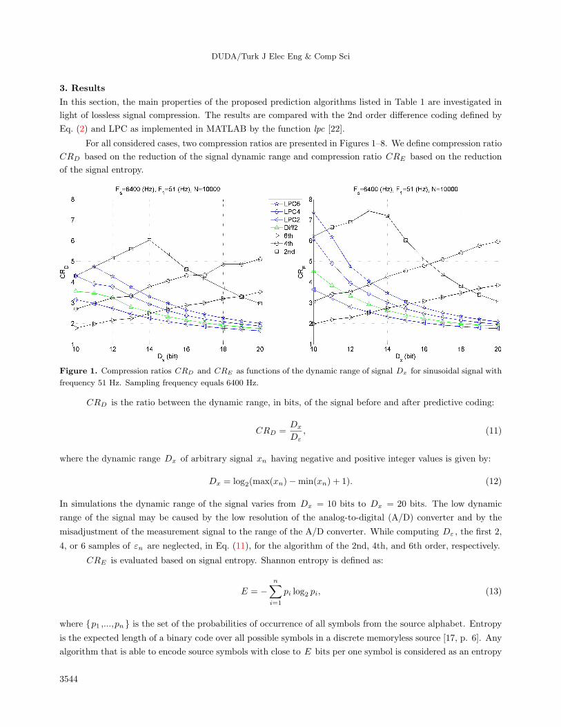
Figure 1. Compression ratios CRD and CRE as functions of the dynamic range of signal Dx for sinusoidal signal with

frequency 51 Hz. Sampling frequency equals 6400 Hz.

CRD is the ratio between the dynamic range, in bits, of the signal before and after predictive coding:

CRD =Dx

Dε, (11)

where the dynamic range Dx of arbitrary signal xn having negative and positive integer values is given by:

Dx = log2(max(xn)−min(xn) + 1). (12)

In simulations the dynamic range of the signal varies from Dx = 10 bits to Dx = 20 bits. The low dynamic

range of the signal may be caused by the low resolution of the analog-to-digital (A/D) converter and by the

misadjustment of the measurement signal to the range of the A/D converter. While computing Dε , the first 2,

4, or 6 samples of εn are neglected, in Eq. (11), for the algorithm of the 2nd, 4th, and 6th order, respectively.

CRE is evaluated based on signal entropy. Shannon entropy is defined as:

E = −n∑

i=1

pi log2 pi, (13)

where {p1 ,...,pn } is the set of the probabilities of occurrence of all symbols from the source alphabet. Entropy

is the expected length of a binary code over all possible symbols in a discrete memoryless source [17, p. 6]. Any

algorithm that is able to encode source symbols with close to E bits per one symbol is considered as an entropy

3544

DUDA/Turk J Elec Eng & Comp Sci

encoder. The most popular entropy encoders are the Huffman coder and the arithmetic coder, both described

in many available textbooks, e.g., [16,17].

The entropy-based compression ratio CRE is defined as the number of bits per one symbol in the original

signal divided by the entropy of the prediction error (i.e. the number of bits per one symbol after predictive

coding and entropy coding):

CRE =Dx

Eε. (14)

While computing Eε , the first 2, 4, or 6 samples of εn are neglected for the algorithm of the 2nd, 4th, and 6th

order, respectively.

CRD is obtained by predictive coding alone that may be used in systems with low computational resources

or high time demands. CRE is a close estimation of what could be obtained if the prediction error was

additionally encoded by entropy coder. This compression is well suited for the offline mode without high time

demands.

In the following, we analyze the coding performance with respect to sampling frequency value, off-nominal

frequency, harmonic distortion, simultaneous amplitude and frequency deviation, and the additive Gaussian

noise. The results are depicted in Figures 1–8. Each figure shows CRD and CRE as a function of the dynamic

range of the signal that varies from Dx = 10 bits to Dx = 20 bits. The curves show the results obtained for

the 6th order LPC (denoted by LPC6), the 4th order LPC (LPC4), the 2nd order LPC (LPC2), the 2nd order

differences defined by Eq. (2) (denoted by Diff2), and the proposed algorithms of the 6th, the 4th, and the 2nd

order (denoted by 6th, 4th, and 2nd). The prediction coefficients for the proposed algorithms are computed for

the nominal system frequency equal to 50 Hz, not for the actual frequency of the signal.

3.1. Sampling frequency

The range of sampling frequencies used in electric power measurements is quite broad. In all further simulations

the results are given for Fs = 6.4 kHz (128 samples per 50 Hz period) and Fs = 50 kHz (1000 samples per

50 Hz period).

3.2. Off-nominal frequency

Figures 1 and 2 show compression results for the sinusoidal signal with frequency 51 Hz. It is observed in

Figure 1 that, for Fs = 6.4 kHz, the proposed 2nd order predictor outperforms all other algorithms for the

dynamic range of the signal Dx lower than approximately 17 bits, and above this value the best results are

obtained by the proposed 4th order predictor. The performance of the 2nd order differences is significantly

worse than the performance of the proposed 2nd order predictor.

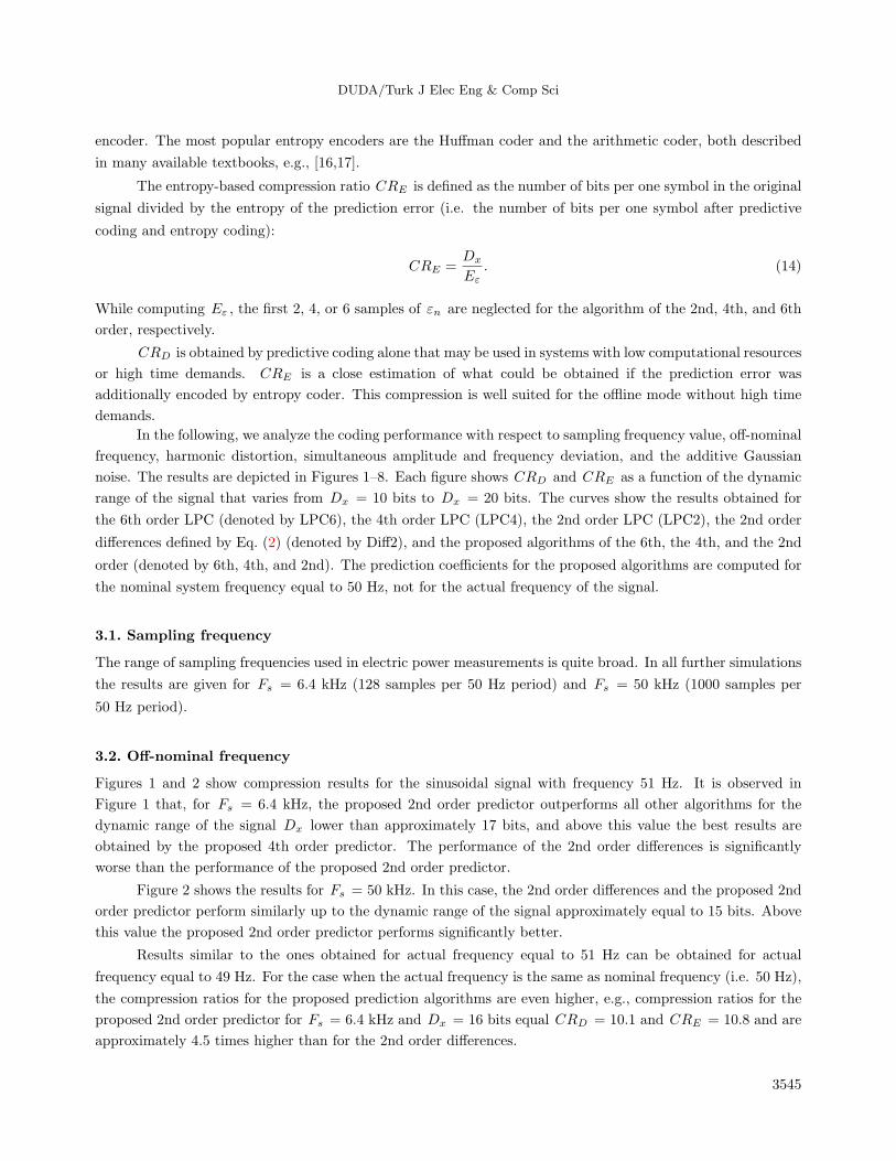
Figure 2 shows the results for Fs = 50 kHz. In this case, the 2nd order differences and the proposed 2nd

order predictor perform similarly up to the dynamic range of the signal approximately equal to 15 bits. Above

this value the proposed 2nd order predictor performs significantly better.

Results similar to the ones obtained for actual frequency equal to 51 Hz can be obtained for actual

frequency equal to 49 Hz. For the case when the actual frequency is the same as nominal frequency (i.e. 50 Hz),

the compression ratios for the proposed prediction algorithms are even higher, e.g., compression ratios for the

proposed 2nd order predictor for Fs = 6.4 kHz and Dx = 16 bits equal CRD = 10.1 and CRE = 10.8 and are

approximately 4.5 times higher than for the 2nd order differences.

3545

DUDA/Turk J Elec Eng & Comp Sci

Figure 2. Compression ratios CRD and CRE as functions of the dynamic range of signal Dx for sinusoidal signal with

frequency 51 Hz. Sampling frequency equals 50 kHz.

3.3. Harmonic distortion

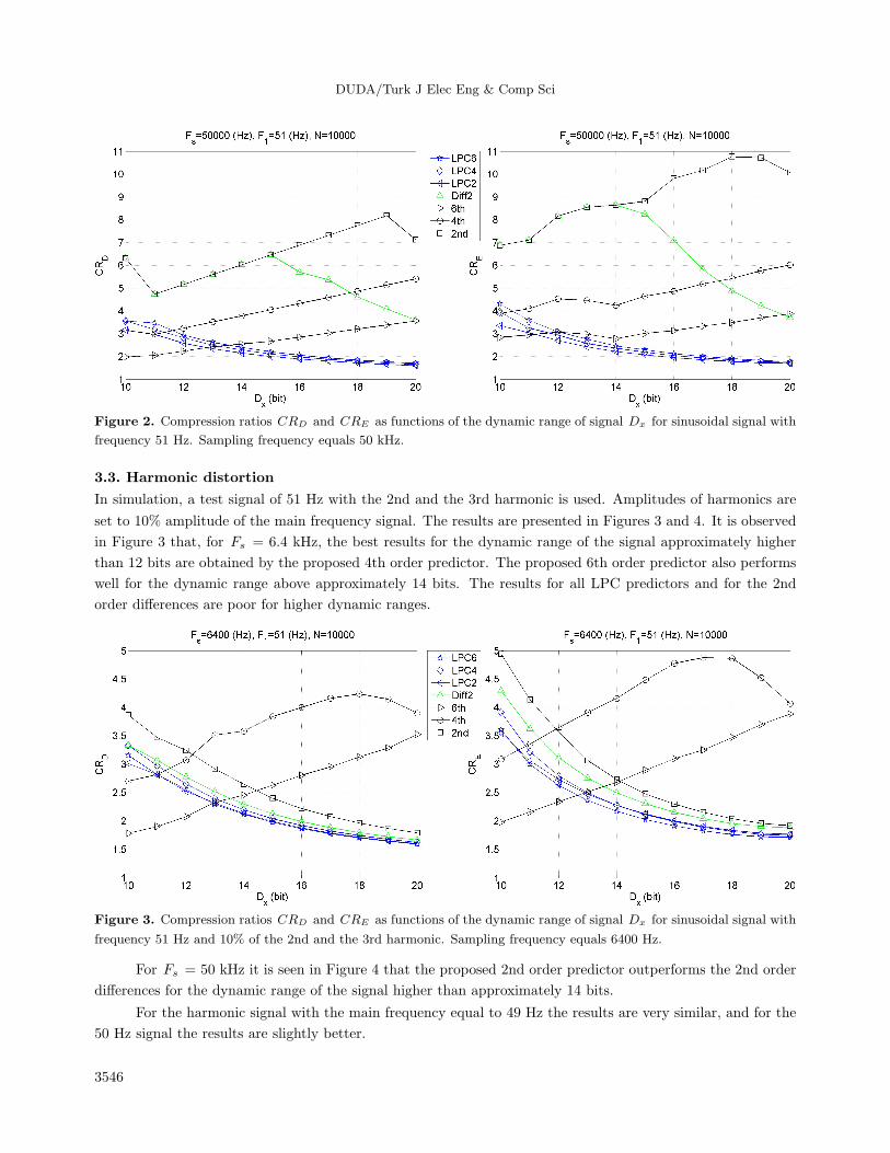
In simulation, a test signal of 51 Hz with the 2nd and the 3rd harmonic is used. Amplitudes of harmonics are

set to 10% amplitude of the main frequency signal. The results are presented in Figures 3 and 4. It is observed

in Figure 3 that, for Fs = 6.4 kHz, the best results for the dynamic range of the signal approximately higher

than 12 bits are obtained by the proposed 4th order predictor. The proposed 6th order predictor also performs

well for the dynamic range above approximately 14 bits. The results for all LPC predictors and for the 2nd

order differences are poor for higher dynamic ranges.

Figure 3. Compression ratios CRD and CRE as functions of the dynamic range of signal Dx for sinusoidal signal with

frequency 51 Hz and 10% of the 2nd and the 3rd harmonic. Sampling frequency equals 6400 Hz.

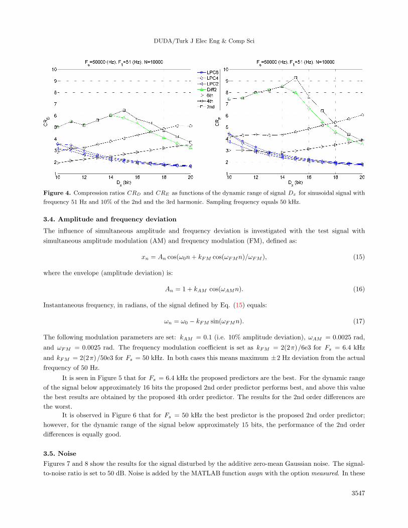
For Fs = 50 kHz it is seen in Figure 4 that the proposed 2nd order predictor outperforms the 2nd order

differences for the dynamic range of the signal higher than approximately 14 bits.

For the harmonic signal with the main frequency equal to 49 Hz the results are very similar, and for the

50 Hz signal the results are slightly better.

3546

DUDA/Turk J Elec Eng & Comp Sci

Figure 4. Compression ratios CRD and CRE as functions of the dynamic range of signal Dx for sinusoidal signal with

frequency 51 Hz and 10% of the 2nd and the 3rd harmonic. Sampling frequency equals 50 kHz.

3.4. Amplitude and frequency deviation

The influence of simultaneous amplitude and frequency deviation is investigated with the test signal with

simultaneous amplitude modulation (AM) and frequency modulation (FM), defined as:

xn = An cos(ω0n+ kFM cos(ωFMn)/ωFM ), (15)

where the envelope (amplitude deviation) is:

An = 1 + kAM cos(ωAMn). (16)

Instantaneous frequency, in radians, of the signal defined by Eq. (15) equals:

ωn = ω0 − kFM sin(ωFMn). (17)

The following modulation parameters are set: kAM = 0.1 (i.e. 10% amplitude deviation), ωAM = 0.0025 rad,

and ωFM = 0.0025 rad. The frequency modulation coefficient is set as kFM = 2(2π)/6e3 for Fs = 6.4 kHz

and kFM = 2(2π)/50e3 for Fs = 50 kHz. In both cases this means maximum ±2 Hz deviation from the actual

frequency of 50 Hz.

It is seen in Figure 5 that for Fs = 6.4 kHz the proposed predictors are the best. For the dynamic range

of the signal below approximately 16 bits the proposed 2nd order predictor performs best, and above this value

the best results are obtained by the proposed 4th order predictor. The results for the 2nd order differences are

the worst.

It is observed in Figure 6 that for Fs = 50 kHz the best predictor is the proposed 2nd order predictor;

however, for the dynamic range of the signal below approximately 15 bits, the performance of the 2nd order

differences is equally good.

3.5. Noise

Figures 7 and 8 show the results for the signal disturbed by the additive zero-mean Gaussian noise. The signal-

to-noise ratio is set to 50 dB. Noise is added by the MATLAB function awgn with the option measured. In these

3547

DUDA/Turk J Elec Eng & Comp Sci

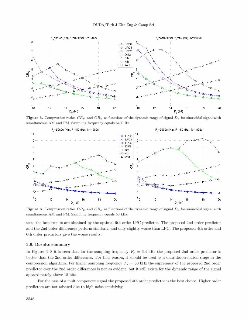
Figure 5. Compression ratios CRD and CRE as functions of the dynamic range of signal Dx for sinusoidal signal with

simultaneous AM and FM. Sampling frequency equals 6400 Hz.

Figure 6. Compression ratios CRD and CRE as functions of the dynamic range of signal Dx for sinusoidal signal with

simultaneous AM and FM. Sampling frequency equals 50 kHz.

tests the best results are obtained by the optimal 6th order LPC predictor. The proposed 2nd order predictor

and the 2nd order differences perform similarly, and only slightly worse than LPC. The proposed 4th order and

6th order predictors give the worse results.

3.6. Results summary

In Figures 1–8 it is seen that for the sampling frequency Fs = 6.4 kHz the proposed 2nd order predictor is

better than the 2nd order differences. For that reason, it should be used as a data decorrelation stage in the

compression algorithm. For higher sampling frequency Fs = 50 kHz the supremacy of the proposed 2nd order

predictor over the 2nd order differences is not as evident, but it still exists for the dynamic range of the signal

approximately above 15 bits.

For the case of a multicomponent signal the proposed 4th order predictor is the best choice. Higher order

predictors are not advised due to high noise sensitivity.

3548

DUDA/Turk J Elec Eng & Comp Sci

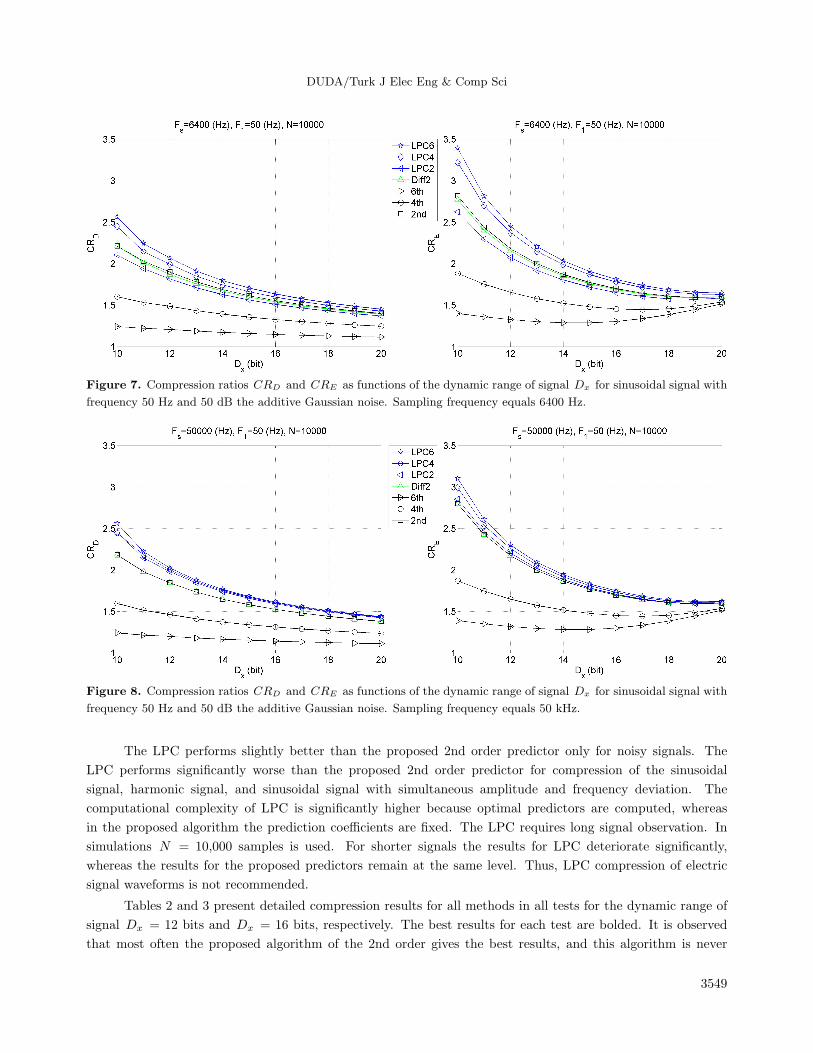
Figure 7. Compression ratios CRD and CRE as functions of the dynamic range of signal Dx for sinusoidal signal with

frequency 50 Hz and 50 dB the additive Gaussian noise. Sampling frequency equals 6400 Hz.

Figure 8. Compression ratios CRD and CRE as functions of the dynamic range of signal Dx for sinusoidal signal with

frequency 50 Hz and 50 dB the additive Gaussian noise. Sampling frequency equals 50 kHz.

The LPC performs slightly better than the proposed 2nd order predictor only for noisy signals. The

LPC performs significantly worse than the proposed 2nd order predictor for compression of the sinusoidal

signal, harmonic signal, and sinusoidal signal with simultaneous amplitude and frequency deviation. The

computational complexity of LPC is significantly higher because optimal predictors are computed, whereas

in the proposed algorithm the prediction coefficients are fixed. The LPC requires long signal observation. In

simulations N = 10,000 samples is used. For shorter signals the results for LPC deteriorate significantly,

whereas the results for the proposed predictors remain at the same level. Thus, LPC compression of electric

signal waveforms is not recommended.

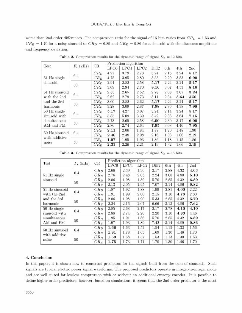
Tables 2 and 3 present detailed compression results for all methods in all tests for the dynamic range of

signal Dx = 12 bits and Dx = 16 bits, respectively. The best results for each test are bolded. It is observed

that most often the proposed algorithm of the 2nd order gives the best results, and this algorithm is never

3549

DUDA/Turk J Elec Eng & Comp Sci

worse than 2nd order differences. The compression ratio for the signal of 16 bits varies from CRD = 1.53 and

CRE = 1.70 for a noisy sinusoid to CRD = 6.89 and CRE = 9.86 for a sinusoid with simultaneous amplitude

and frequency deviation.

Table 2. Compression results for the dynamic range of signal Dx = 12 bits.

Test Fs (kHz) CRPrediction algorithmLPC6 LPC4 LPC2 Diff2 6th 4th 2nd

6.4CRD 4.27 3.79 2.73 3.24 2.16 3.24 5.17

51 Hz single CRE 4.75 3.95 2.80 3.33 2.29 3.53 6.90sinusoid

50CRD 2.94 2.82 2.58 5.17 2.24 3.24 5.17CRE 3.09 2.94 2.70 8.16 3.07 4.53 8.16

51 Hz sinusoid6.4

CRD 2.55 2.65 2.52 2.78 2.08 3.07 3.24with the 2nd CRE 2.62 2.79 2.73 3.11 2.34 3.64 3.56and the 3rd

50CRD 3.00 2.82 2.62 5.17 2.24 3.24 5.17

harmonic CRE 3.28 3.09 2.87 7.98 2.96 4.38 7.9850 Hz single

6.4CRD 5.17 4.27 3.07 3.24 2.14 3.24 5.17

sinusoid with CRE 5.85 5.09 3.39 3.42 2.33 3.64 7.15simultaneous

50CRD 2.73 2.65 2.58 6.00 2.30 3.47 6.00

AM and FM CRE 2.86 2.74 2.64 7.95 3.08 4.46 7.95

50 Hz sinusoid 6.4CRD 2.11 2.06 1.84 1.87 1.20 1.48 1.90

with additiveCRE 2.46 2.38 2.08 2.16 1.33 1.66 2.19

noise 50CRD 1.97 1.95 1.93 1.86 1.18 1.45 1.86CRE 2.31 2.26 2.21 2.19 1.32 1.66 2.19

Table 3. Compression results for the dynamic range of signal Dx = 16 bits.

Test Fs (kHz) CRPrediction algorithmLPC6 LPC4 LPC2 Diff2 6th 4th 2nd

6.4CRD 2.66 2.39 1.96 2.17 2.88 4.32 4.63

51 Hz single CRE 2.76 2.48 2.03 2.24 3.08 4.80 5.10sinusoid

50CRD 2.06 1.98 1.89 5.70 2.85 4.32 6.89CRE 2.13 2.05 1.95 7.07 3.14 4.86 9.82

51 Hz sinusoid6.4

CRD 1.87 1.92 1.88 1.99 2.81 4.00 2.22with the 2nd CRE 1.91 1.99 2.00 2.15 3.10 4.78 2.30and the 3rd

50CRD 2.06 1.98 1.90 5.33 2.85 4.32 5.70

harmonic CRE 2.24 2.16 2.07 6.66 3.13 4.86 7.6250 Hz single

6.4CRD 2.85 2.68 2.17 2.17 2.78 4.10 4.10

sinusoid with CRE 2.88 2.74 2.20 2.20 3.10 4.83 4.46simultaneous

50CRD 1.95 1.91 1.86 5.70 2.85 4.32 6.89

AM and FM CRE 1.97 1.93 1.89 7.42 3.14 4.89 9.86

50 Hz sinusoid 6.4CRD 1.66 1.63 1.52 1.54 1.15 1.32 1.56

with additiveCRE 1.81 1.78 1.65 1.69 1.30 1.46 1.70

noise 50CRD 1.59 1.58 1.57 1.53 1.13 1.30 1.53CRE 1.75 1.73 1.71 1.70 1.30 1.46 1.70

4. Conclusion

In this paper, it is shown how to construct predictors for the signals built from the sum of sinusoids. Such

signals are typical electric power signal waveforms. The proposed predictors operate in integer-to-integer mode

and are well suited for lossless compression with or without an additional entropy encoder. It is possible to

define higher order predictors; however, based on simulations, it seems that the 2nd order predictor is the most

3550

DUDA/Turk J Elec Eng & Comp Sci

versatile algorithm. The highest increase of the compression ratio obtained by the proposed 2nd order predictor

with respect to the 2nd order differences equals approximately 2.4 times for sampling frequency of 6.4 kHz and

14 bits dynamic range of the signal, and approximately 2 times for sampling frequency of 50 kHz and 19 bits

dynamic range of the signal. The obtained improvements are significant for the case of lossless compression.

Acknowledgment

This work was supported by the National Centre for Research and Development (NCBiR) under agreement

PBS1/A4/6/2012.

References

[1] Duda K, Zielinski TP. FIR filters compliant with the IEEE standard for M class PMU. Metrol Meas Syst 2016; 23:

623-636.

[2] Borkowski D, Wetula A, Bien A. New method for noninvasive measurement of utility harmonic impedance. In:

IEEE 2012 Power and Energy Society General Meeting; 22–26 July 2012; San Diego, CA, USA. New York, NY,

USA: IEEE. pp. 1-8.

[3] Vural B, Kızıl A, Uzunoglu M. A power quality monitoring system based on MATLAB server pages. Turk J Elec

Eng & Comp Sci 2010; 18: 313-325.

[4] Kocatepe C, Kekezoglu B, Bozkurt A, Yumurtacı R, Inan A, Arıkan O, Baysal M, Akkaya Y. Survey of power

quality in Turkish national transmission network. Turk J Elec Eng & Comp Sci 2013; 21: 1880-1892.

[5] Lisowski M. Lossless voltage data compression for power quality analysis–a Huffman–delta approach. In: IEEE 2013

Signal Processing: Algorithms, Architectures, Arrangements, and Applications; 26–28 September 2013; Poznan,

Poland. New York, NY, USA: IEEE. pp. 133-136.

[6] Tcheou MP, Lovisolo L, Ribeiro MV, da Silva EAB, Rodrigues MAM, Romano JMT, Diniz PSR. The compression

of electric signal waveforms for smart grids: state of the art and future trends. IEEE T Smart Grid 2014; 5: 291-302.

[7] Stacchini de Souza JC, Assis TML, Pal BC. Data compression in smart distribution systems via singular value

decomposition. IEEE T Smart Grid 2017; 8: 275-284.

[8] Loia V, Tomasiello S, Vaccaro A. Fuzzy transform based compression of electric signal waveforms for smart grids.

IEEE T Syst Man Cyb Cy A 2017; 47: 121-132.

[9] Tong X, Kang C, Xia Q. Smart metering load data compression based on load feature identification. IEEE T Smart

Grid 2016; 7: 2414-2422.

[10] Cormane J, Nascimento FAO. Spectral shape estimation in data compression for smart grid monitoring. IEEE T

Smart Grid 2016; 7: 1214-1221.

[11] Khan J, Bhuiyan SMA, Murphy G, Arline M. Embedded-zerotree-wavelet-based data denoising and compression

for smart grid. IEEE T Ind Appl 2015; 51: 4190-4200.

[12] Tate JE. Preprocessing and Golomb–Rice encoding for lossless compression of phasor angle data. IEEE T Smart

Grid 2016; 7: 718-729.

[13] Unterweger A, Engel D. Lossless compression of high-frequency voltage and current data in smart grids. In IEEE

2016 International Conference on Big Data; 5–8 December 2016; Washington, DC, USA. New York, NY, USA:

IEEE. pp. 3131-3139.

[14] Bien A, Borkowski D, Wetula A. Estimation of power system parameters based on load variance observations -

laboratory studies. In: IEEE 2007 Electrical Power Quality and Utilisation International Conference; 9–11 October

2007; Barcelona, Spain. New York, NY, USA: IEEE. pp. 1-6.

[15] Borkowski D, Barczentewicz S. Power grid impedance tracking with uncertainty estimation using two stage weighted

least squares. Metrol Meas Syst 2014; 21: 99-110.

3551

DUDA/Turk J Elec Eng & Comp Sci

[16] Salomon D. Data Compression: The Complete Reference. 3rd ed. New York, NY, USA: Springer, 2004.

[17] Acharya T, Tsai PS. JPEG2000 Standard for Image Compression Concepts, Algorithms and VLSI Architectures.

Hoboken, NJ, USA: Wiley & Sons, 2005.

[18] Zhang D, Bi Y, Zhao J. A new data compression algorithm for power quality online monitoring. In: IEEE 2009

Sustainable Power Generation and Supply International Conference; 6–7 April 2009, Nanjing, China. New York,

NY, USA: IEEE. pp. 1-4.

[19] Duda K. Lifting based compression algorithm for power system signals. Metrol Meas Syst 2008; 15: 69-83.

[20] Duda K. Integer fast Fourier transform - implementation and application. In: IEEE 2004 12th European Signal

Processing Conference; 6–10 September 2004; Vienna, Austria. New York, NY, USA: IEEE. pp. 1517-1520.

[21] Jackson LB. Digital Filters and Signal Processing. 2nd ed. Dordrecht, the Netherlands: Kluwer Academic Publishers,

1989.

[22] MathWorks. Signal Processing Toolbox User’s Guide. Natick, MA, USA: The MathWorks, Inc., 2006.

[23] Vaidyanathan PP. The Theory of Linear Prediction. San Rafael, CA, USA: Morgan & Claypool, 2008.

[24] Zielinski TP, Duda K. Frequency and damping estimation methods–an overview. Metrol Meas Syst 2011; 18: 505-

528.

[25] Duda K, Zielinski TP. Efficacy of the Frequency and damping estimation of real-value sinusoid. IEEE Instru Meas

Mag 2013; 16: 48-58.

[26] Borkowski D, Bien A. Improvement of accuracy of power system frequency analysis by coherent resampling. IEEE

T Power Deliver 2009; 24: 1004-1013.

3552