Low-Cost Real-Time License Plate Recognition for

a Vehicle PC

ERIK BERGENUDD

Master’s Degree Project

Stockholm, Sweden December 2006

XR-EE-SB 2006:023

© Erik Bergenudd, December 2006 KTH Signaler, sensorer och system SE-100 44 Stockholm SWEDEN XR-EE-SB 2006:023

iii

Abstract This thesis develops an algorithm for automatic license plate recognition

(ALPR). ALPR has gained much interest during the last decade along with the improvement of digital cameras and the gain in computational capacity. Earlier character recognition has been used in structured processes like bank cheque processing. Now the ability of recognising car license plates has gained interest. ALPR can be used in many areas from speed enforcement and toll collection to management of parking lots where the ability to recognise the identity of each car accurately provides the number of cars and the parking time of each car. The algorithm developed here is aimed to be lightweight so that it can be run on board a car in real-time. With images provided by a USB web-camera (with modified optics), the system will be able to recognise Swedish standard license plates under normal conditions.

The algorithm is built in three sections; the first is the initial detection of a possible license plate using edge and intensity features in the image; in the second, the text of the plate is found and normalized; last is the actual character recognition. The first step uses edge and intensity detection to extract information from the image. The information is then combined into segments, which are evaluated for the likeliness of containing a plate. The second step evaluates the selected segment to find the position and orientation of the plate. The plate is then rotated to horizontal alignment and normalized. The last step reads the characters by correlation template matching. Template matching is a simple but robust way of recognising structured text with a small set of characters.

The resulting implementation can successfully recognise Swedish standard license plates with a frame rate of around 10 frames per second. It manages different relative sizes of the plate in the picture, from very large to small plates of height about 20 pixels. The algorithm is though inferior recognising unevenly illuminated plates or plates with bright white surroundings such as snow. It utilises the match information from consecutive frames for decision support.

iv

v

Contents

Chapter 1 - Introduction .............................................................................1 1.1 Introduction to the topic ...............................................................1 1.2 Automatic License Plate Recognition ...........................................1 1.3 Thesis formulation .......................................................................2 1.4 Thesis Report Outline ..................................................................3

Chapter 2 - System model ...........................................................................5

2.1 Basic Concepts .............................................................................5 2.2 Structure of the Process ................................................................6 2.3 White Intensity Detection .............................................................7 2.4 Colour Edge Detection .................................................................7 2.5 Morphological Operations ............................................................8 2.6 Segmentation and Merging ..........................................................9 2.7 Hough Transform .......................................................................10 2.8 Rotation of the Image .................................................................10 2.9 Final Extraction and Normalization ............................................11 2.10 Optical Character Recognition .................................................12 2.11 Sequencing ..............................................................................13 2.12 Super-resolution .......................................................................14

Chapter 3 - Implementation ......................................................................15

3.1 Initial Considerations .................................................................15 3.2 Localization ...............................................................................15 3.3 Colour Edge Detection ...............................................................15 3.4 Intensity Binarization .................................................................17 3.5 Morphological Operations ..........................................................18 3.6 Segmentation .............................................................................19 3.7 Hough Transformation ...............................................................20 3.8 Affine Transformations ..............................................................22 3.9 Optical Character Recognition ...................................................24 3.10 Feature extraction .....................................................................25 3.11 Contrast enhancement ..............................................................27 3.12 Sequencing ..............................................................................28 3.13 Design Parameters .............................................. .......................29

Chapter 4 - Results ...................................................................................31

4.1 Future Work ...............................................................................32 References ................................................................................................35 Appendix A ..............................................................................................37

A.1 The Hough Transform ...............................................................37

vi

List of Figures

1.1 The mobile testbed TRÖGE...................................................................2 1.2 SMS replies from Swedish Road Administration ...................................3 2.1 Sample picture in full and work resolution.............................................5 2.2 Process structure flowchart ....................................................................6 2.3 Edge and intensity maps ........................................................................7 2.4 Edge and intensity maps after morphological operations........................9 2.5 Schematic view of bilinear rotation......................................................11 2.6 Examples of rotated and scaled pixel grids...........................................12 3.1 Segmented pictures..............................................................................20 3.2 The steps preceding Hough transform..................................................21 3.3 Detailed view of bilinear rotation.........................................................23 3.4 Character Templates with features marked...........................................26 3.5 Contrast enhancement..........................................................................28 3.6 Sequencing system ..............................................................................29 4.1 Screen-shot of the implementation.......................................................32 A.1 Example image with corresponding Hough plot..................................37

1

Chapter 1 - Introduction

1.1 Introduction to the topic During many years techniques to read text automatically have been developed.

First out were the banks that used magnetic ink to speed up cheque processing. With the development of better scanners and the gain in computer development, the interest for optical character recognition (OCR) has grown. Today there exists very advanced OCR programs that can read almost all written text [1]. The possibility to read structured text in documents has turned the interest to the ability to read texts and symbols in other areas. One such area is the automatic license plate recognition (ALPR), using a camera to take photos of passing vehicles to make is possible to identify them automatically. This thesis project aims at implementing a low-density ALPR system. The system is supposed to be installed into a car and continuously scan for vehicles in front of the car and read their license plates. Such a system could be used for instance in police cars to automatically look for wanted cars or just check the traffic status of the car, or in public buses to prevent misuse of reserved bus lanes etc.

1.2 Automatic License Plate Recognition ALPR is today used commercially in many places. There exist systems used

for car toll collection [2, 3], speed enforcement [4] and for instance to manage parking lots [5]. ALPR can be used almost anywhere to keep track of which or how many cars there are on a specific location, road, etc. These implementations mostly use high quality single shot cameras, which are mounted on fixed locations. Other assistance often used are infra-red flash to light up the plate and systems to detect when the car is in a specific location. For instance, the Stockholm trials [3] use laser scanners, which detect when a car is passing and it can distinguish between e.g. cars and motorbikes. A stationary implementation can use high performance computers and often has plenty of time to solve complex algorithms for each captured picture. In a mobile implementation, less performance is available to keep down heat production, size and power consumption. It is also harder to make assumptions about background and the presence of a car. The process of ALPR can basically be divided into three parts:

• to determine the region of interest in which the possible plate is assumed to be located,

• the orientation of the plate must be determined so it can be adjusted and normalized in size,

• an OCR process reads the plate and matches the registration number. These three steps are used by most ALPR implementations, although the algorithms in each step might vary.

2

1.3 Thesis formulation This thesis is a continuation of a previous 10-week “studienarbeit” [6], which

resulted in a C++ implementation. The program from the previous project can successfully read some license plates, although it is not very robust and fails rather often. This thesis uses the source code and theories from the previous project as a start, with the aim of improving the system to achieve an acceptable recognition rate.

The ALPR system is supposed to work automatically without human interaction in real-time. The camera does not know whether a car is present and will therefore continuously provide the system with pictures. No a priori knowledge about the position, size or orientation of the plate will be provided, nor information about the background. The camera delivers pictures of varying quality. Due to long shutter times, motion blur is common, as is blurring due to poor focusing and low focus depth caused by large apertures.

The system is designed to be fitted into a car and automatically read the license

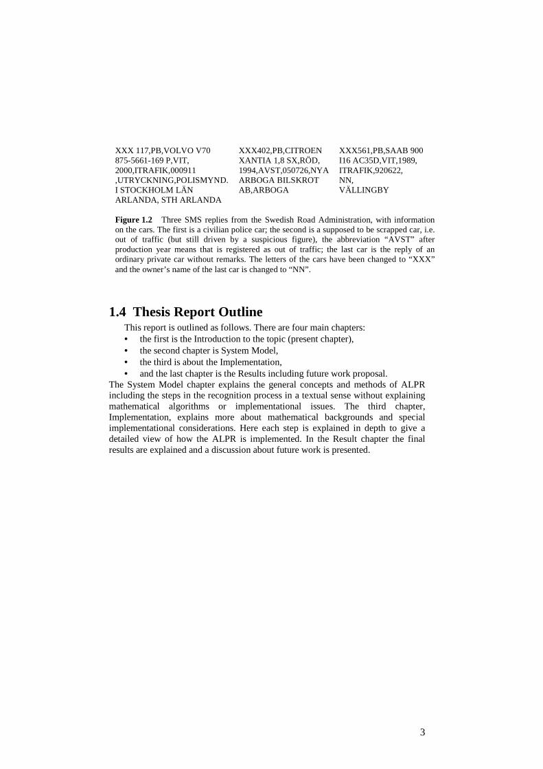
plate of the car in front. The camera is a standard USB webcam modified with new optics to get longer focal length. The system will be integrated into the mobile platform TRÖGE, see Figure 1.1. TRÖGE is a mobile testbed designed to be fitted into a car and perform tasks like GPS aided inertial navigation and ALPR. TRÖGE is based on standard PC components and it has a small touch screen (7”) for user input. It also supports USB, Wi-Fi networks and it has a GSM/GPRS modem. The GSM modem can be used to communicate the license plate number via SMS-messaging to the Swedish Road Administration, which returns a SMS with data on the vehicle [7]. The data provided is what kind of car it is, e.g. motor car, bus, truck, motorbike etc, which brand, model and colour it has, production year, traffic status, special status such as if it is stolen, leased, wanted, emergency vehicle etc, name of the owner and residence of the owner. See Figure 1.2 for three samples of SMS replies.

Figure 1.1 The TRÖGE testbed and the modified USB web camera used in this project. The sizes are not comparable, the screen of the TRÖGE testbed is 7 inch and the lens of the camera is standard diameter of 49 mm.

3

1.4 Thesis Report Outline This report is outlined as follows. There are four main chapters: • the first is the Introduction to the topic (present chapter), • the second chapter is System Model, • the third is about the Implementation, • and the last chapter is the Results including future work proposal.

The System Model chapter explains the general concepts and methods of ALPR including the steps in the recognition process in a textual sense without explaining mathematical algorithms or implementational issues. The third chapter, Implementation, explains more about mathematical backgrounds and special implementational considerations. Here each step is explained in depth to give a detailed view of how the ALPR is implemented. In the Result chapter the final results are explained and a discussion about future work is presented.

XXX 117,PB,VOLVO V70 XXX402,PB,CITROEN XXX561,PB,SAAB 900 875-5661-169 P,VIT, XANTIA 1,8 SX,RÖD, I16 AC35D,VIT,1989, 2000,ITRAFIK,000911 1994,AVST,050726,NYA ITRAFIK,920622, ,UTRYCKNING,POLISMYND. ARBOGA BILSKROT NN, I STOCKHOLM LÄN AB,ARBOGA VÄLLINGBY ARLANDA, STH ARLANDA Figure 1.2 Three SMS replies from the Swedish Road Administration, with information on the cars. The first is a civilian police car; the second is a supposed to be scrapped car, i.e. out of traffic (but still driven by a suspicious figure), the abbreviation “AVST” after production year means that is registered as out of traffic; the last car is the reply of an ordinary private car without remarks. The letters of the cars have been changed to “XXX” and the owner’s name of the last car is changed to “NN”.

4

5

Chapter 2 - System model This chapter explains in a general sense the structure of the methods in the

recognition process. It explains the algorithms in a textual sense and does not describe implementational issues.

2.1 Basic Concepts It is important to make the processing as fast as possible, without allowing the

recognition rate to fall. More processed pictures give more data, which in turn gives better support for a good decision, and the faster a picture is processed, the more relevant is the result. In computer processing, the complexity is often countedin required multiplications. To keep the number of operations down is it important to make sure that as few processes as possible are required.

There is however also another effective way of reducing the complexity: by reducing the size of the image, the number of required operations can be cut down significantly. The complexity of most algorithms used in this implementation is of degree n, i.e. a fixed number of multiplications are performed for each pixel in the picture. If the height and the width of the picture are cut by half, just a quarter of the computational time will be required. See Figure 2.1 for an example of the resolution of the acquired input image and the image in work-resolution. Another way of reducing the size of the picture is to optimize the information per pixel. The given picture from the camera is RGB coded with 256 intensity levels, i.e. it uses 8 bits per pixel and colour layer. During the processing, all that information is not always needed. In some levels only a black/white intensity value is needed, in other parts only a binary value representing whether the pixel is on or off. In the latter case, a 1 bit VGA picture requires 38,4 kilobyte (kB), whereas a 8 bit RGB coded picture requires 921,6 kB.

Figure 2.1 Sample picture. Left picture has original input resolution of 640x480 pixels. The right picture has the processing resolution of 128x96 pixels. No smoothing or interpolation is used in the reduction process, just every fifth pixel is extracted to the new picture to keep down processing time. The compressed picture is just used to localize the plate and as can be seen, the resolution is too low even for the human eye to read the characters. When the plate is found it is extracted from the high resolution picture to the left for further processing.

6

Less data speeds up the processing in several ways, it is faster to load and store, smaller variables can be processed faster and with binary values logical operations can be used, which are very fast. This program uses several consequence algorithms on the same picture, which requires loading and storing operations for each algorithm. This means a large gain in processing time if the number of pixels can be kept down.

2.2 Structure of the Process The recognition process is divided into three sections, which each contains a

sequence of related operations. The whole process can be studied in Figure 2.2. The first step in the picture processing is to identify areas that has a good white intensity and contains many shifts from black to white. When a number of such areas, or regions of interest, have been identified, they need to be validated and a primary area be selected. The area which is the most likely to contain a licence plate is cut out and sent on for further processing.

When an area that is likely to contain a plate is found, the plate’s location must be better determined. The way to do this can differs between implementations and in this thesis; the aim is to identify the upper and lower edge of the plate. This is done by performing a Hough transform. The Hough transform can be used to find straight lines in pictures, it can also be used to find other geometric patterns such as circles. The Hough transform results in two straight-line equations and is the first real non-pixel based information known about the plate. With the equations of the lines, assumed to describe the horizontal edges of the plate, the picture can be cut out and rotated along these lines.

Image Acquisition

and Reduction Colour Edge

Detection Intensity

Binarization

Morphological Operator

Morphological Operator

Segmentation Segmentation Merging and Selection

(First Part Done) ROI Obtained

Plate Inclination Detection

(Hough Transform)

Rotation and Scaling

Optical Character Recognition

Final Extraction (Part 2 Done)

Figure 2.2 Flow chart showing the steps in the plate detection and recognition process.

7

For the horizontal plate, is it easy to cut away the white frame so that the picture only contains the characters. Depending on the OCR method, the picture may need to be scaled to a nominal height for easier recognition.

2.3 White Intensity Detection The white intensity detection is used to find areas in the picture that have a

bright white colour. The idea behind the use of this algorithm is that the plate has a very white colour and reflexive background, which lights it up. The use of white-colour intensity detection suppresses the risk of detecting rear lights and other bright items as high intensity areas. The intensity map can either be determined for a fixed threshold, where all pixels more intense than the threshold are marked, or for a percentage threshold. The percentage threshold is calculated as the amount of bright pixels that should be above the threshold. The intensity map is then determined as for the fixed threshold. In Figure 2.3 the intensity map of the right picture from Figure 2.1 can be studied.

2.4 Colour Edge Detection The binary intensity profile is not enough too determine the region of interest

for further work. Another distinctive feature of the license plate is that it contains many edges from white to black and vice versa. An edge detection algorithm finds sharp shifts in intensity of the picture, i.e. edges. When checking for edges that are strong in all colour layers, primarily the black/white edges are found. The colour edge detection is performed as a convolution between the image and the mask horizontal mask, h = [0,5 0 -0,5]. This means that it traverses the picture row by row, takes the value for the preceding pixel and subtracts the value for the following pixel. If the values of all the three colour layers mark an edge, then the pixel will be filled. The horizontal mask does only mark vertical edges, and this does of course give less marked edges than a two dimensional algorithm would do.

Figure 2.3 The left picture is the intensity profile of the processing resolution picture from figure 2.1. All pixels brighter than the 20 % brightest pixels and which have a decent white colour are set. In this specific picture, the license plate is almost missed since there is a large field of very bright snow in the background, which results in a high threshold. Large fields of for instance snow can make the picture unreadable. The right picture is the vertical edge map of the same picture. Here all vertical edges in the picture are marked. The licence plate is easily seen as a marked rectangle.

8

The plate does however contain many vertical edges and by only searching for edges in one dimension, much computational time is saved. By only marking black/white edges, less relevant edges are excluded. In Figure 2.3 the edge map of the sample picture from Figure 1.1 can be studied.

2.5 Morphological Operations The intensity map is a binary picture containing scattered pixels marking bright

items and individual pixels that are noise. In addition, the edge map can contain much noise from small irrelevant edges. To get rid of some noise and to get the marked pixels around the plate connected, two algorithms called dilation and erosion are used. These algorithms are also called morphological operators. The algorithms take advantage of the fact that in the area of the plate, the marked pixels are closer to each other than in other parts of the picture. The order between these algorithms is very important since the reversed process would give a completely different result. The process to perform first dilation and then erosion with the same mask is called a morphological closing operation, the reverse is called opening operation. In this implementation, the masks are altered between dilation and erosion, why the result is just similar to the closing operation. The dilation process uses a mask, or a structuring element, which can have different size and pattern for different tasks. The algorithm fills a pixel if the mask centred over that pixel covers one or more set pixels in the input picture. The result is that holes in fields of marked pixels are filled and areas of filled pixels grow. Areas closer to each other than the size of the mask are connected. After the dilation is performed, an erosion algorithm is used on the result. The erosion is the opposite of the dilation. It does also use a structuring element, but it only marks pixels if all pixels covered by the mask are set. In this combination, the erosion mask is slightly larger than the dilation mask. The result is that areas connected only by a thin line of pixels are disconnected, that small sets of pixels are erased and the areas of marked pixels shrink. See Figure 2.4 for samples of the dilated picture and the result after the closing operator. Both the intensity map and the edge map are processed with the operators although the size of the mask differs between them. The final binary images look similar to each other, although they in the optimal case mark different areas except for the license plate, which both pictures should mark.

9

2.6 Segmentation and Merging When both the edge and the intensity maps are calculated, it is time to combine

the results. However, before the pictures can be combined they need to be more structured. Therefore, the pictures will be segmented, meaning that all fields of connected pixels are joined into numbered segments. The segmenting process goes through the binary picture and creates rectangular segments boxing in all connected pixels in an area. The segments are numbered and listed with their size and position. Two segments in the same picture may overlap each other. For instance in the upper left corner of picture c. in Figure 2.4, there is a large ‘c’-shaped field that will give a large square segment. This will overlap the small line segment in the middle of the ‘c’ opening. The reason not to merge these segments is to keep down the size of the interesting regions. When lists of the segments in the two pictures are produced, they can be combined so that segments from the two pictures that overlap each other are combined to create a region of interest (ROI). The ROI will have the size of the area that both segments cover. Segments that do not have a corresponding overlapping segment in the other picture are discarded. The details of the segmentation and merging process used in this implementation will be further explained in the Implementation chapter, section 3.6.

Often several ROIs are detected. Then one must be selected as the best and most probable to contain a plate. Criteria that can be used for selection are for instance the size and the amount and intensity of edges. When only one ROI is left, then that area is cut out from the original high-resolution picture for further processing.

a b

c Figure 2.4 Image b. shows the edge map from Figure 2.2 after the dilation operation is performed. As can be seen has the process stretched out all pixels in horizontal direction to connect neigh-bouring pixels. Image c. shows the dilated edge map after the erosion operator. This has reduced the size of all fields such that only fields originating from strongly edged areas are left. The plate can be seen as the rectangle in the middle. Image a. is the intensity map after both operations. Almost only the strong snow fields are left marked, of the plate only a single lone pixel in the middle remains.

10

2.7 Hough transform The license plate in the final ROI from the previous part has an inclination and

a size that is unknown. The purpose of the following steps is to extract the plate so that the picture just contains the characters and almost no parts of the white border. The first problem is to find the inclination of the plate and rotate the picture to an exact horizontal alignment. To determine the angle of which the plate is aligned, a process called Hough transform is used. To give a useful input for the Hough transform, edge detection is performed again. This time the edge detection is run column-wise in the picture to create a binary image with horizontal edges, such as the upper and lower edge of the plate, marked. The edge map is eroded using the erosion function to remove noise such as edges of the characters. The Hough transform works in the way that for every pixel set in the edge map, it creates a sine curve in Hough space as a direct mapping from the pixels coordinates. It creates a line for each pixel as long as the angular resolution demands. If all angles from 0 to 2 π radians are interesting and a resolution of 0.01 radians is needed, a 630 pixels long Hough space plot would have to be created. In this application, the size can be reduced severely due to the fact that licence plates normally are aligned almost horizontal. When lines have been drawn for all pixels, the Hough-space plot can be analysed. The strongest value in the plot corresponds to the strongest line in the original picture, with a direct mapping from the coordinates of the spot to that line’s equation. Now the angle and the equations of the lines of the upper and lower borders of the plate are known. See Appendix A for further details on the Hough transform.

2.8 Rotation of the Image To rotate the image, from its skewed form to a horizontal aligned form, a

mapping between two coordinate systems must be performed. This is a computationally nontrivial task. In a pixel-based picture, the individual pixels can be seen as squares with a specified area. The problem, when rotating, is that one pixel in the source picture cannot be directly mapped to a pixel in the destination grid with a good result. Due to the angular alignment, the source pixels will cover parts of normally four destination pixels, which all need a part of the contribution. See Figure 2.6 for an example of how larger pixel-grids intersect each other and how the areas of contribution vary in different parts when rotation is performed. In Figure 2.5 the mapping from the source pixels to a destination pixel is showed in detail. It is difficult to calculate the exact area of the coverage at each destination pixel, why there is much room for optimizations here. The most trivial implementation is the nearest neighbour approach, which means that the source pixel is assigned to the destination pixel, which it covers the most. This gives a pour result, especially in low resolution images were lines would be clearly disrupted when the nearest destination pixel moves from one row to the next, also called aliasing. This can be improved by using different kinds of interpolation. One way to make a simple improvement, that for smaller angular adjustments usually gives a good result, is to interpolate between the two closest pixels in x or y direction depending on which axis is used as a reference. Still, cuts will be found in straight lines, but just in one direction. In the other direction, the result will be smoothened lines. A final solution for a simple mapping algorithm can therefore be to interpolate between the four closest destination pixels, although there can be

11

cases with other constellations then that of four covered pixels and distortion will occur. This is also called bilinear interpolation [8, p 273].

2.9 Final Extraction and Normalization When the picture is horizontally aligned, the characters can be cut out. By

creating horizontal and vertical histograms over the picture, the darker characters can be distinguished from the white background border. The resulting image contains just the six characters of the plate and as little of the surrounding plate as possible. A last task before OCR is to normalize the size of the characters. The OCR method used in this implementation requires that the characters have a predefined size matching the templates. The height of the plate is used as size reference since it is easier to isolate and remove the white border above and below the characters, than it is to find the left and right border of the plate. The scaling is performed using bilinear interpolation. The method is the same as in the previous rotation, though the exact areas of the different covered pixels can be calculated, since the coverage of the new pixels on the old grid forms regular squares. See Figure 2.6 for an example of how pixel-grids intersect each other when scaling. Important to notice is that the picture can be both enlarged and reduced in size. The latter case is most common in this implementation, where the normalized height is set to twenty pixels, but in some cases, an enlargement is required.

Pd

Ps.1

Ps.2

Ps.3

Ps.4

Pd

Destination pixel

Contribution area of source pixel Ps.1

Contribution area of source pixel Ps.2

Contribution area of source pixel Ps.3

Contribution area of source pixel Ps.4

Source pixels

Figure 2.5 Picture describing how the source pixels are mapped to the destination picture (yellow) when the rotation is performed. The area of the coverage is estimated as a square from the position of the corner instead of calculating the exact area of the skewed quadrangle. The distortion increases the further from the middle of the destination pixel the centre of the source pixels get.

12

2.10 Optical Character Recognition There exist many techniques to perform OCR. The simplest way is to compare

the picture with template pictures of each character and choose the most likely one. This method is suitable to recognize highly structured text like in ALPR, where the font is known and the characters are structured with equal spacing and size together with a limited number of letters. If more fonts or possible characters and sizes were supposed to be recognizable, the number of templates to match with would grow fast and with that the computational time as well as the risk of a mismatch. To support the template match decisions, simple feature extracting can be suitable to use. For instance, if it is hard to distinguish between F and P, extra care should be taken to check the area of the P’s arc. Methods that are more sophisticated can analyse the characters to find features like arcs, lines and circles, which combined, together forms the pattern of a certain letter. That method is more independent of size and font of the character, but it is on the other hand more sensible to noise. Many OCR techniques use knowledge about spelling and grammar to support their decision in difficult cases. In ALPR most combinations of letters can occur (some combinations of letters are not used since they might be offending, but they are rather few and a check against such a list would correct very few decisions). The only assumption on the plate will therefore be that it contains three letters followed by a space for the tax mark and then three digits.

The present implementation will use the simple and robust method of comparing the plate with predefined templates. The comparison is done with normalized correlation calculation to get the degree of match. The Swedish license plates use all the ten numbers, but only 23 letters, since only capital letters are used and I, V and Q as well as Å, Ä, Ö are excluded due to the risk of misinterpretations. There also exist personal plates, which have a text of two to seven characters, letters or digits to form an individually selected word such as the owner’s nickname. Some plates have a different background colour: taxis – yellow, diplomatic cars - blue (plus a different character layout) and sale cars - green [9].

Figure 2.6 An example showing how pixels in a source grid (red) are mapped onto several pixels in a destination grid when rotation and scaling is performed. In both cases, some kind of interpolation must be used to calculate the new pixel magnitudes to avoid distortions in the output picture.

13

These will be difficult to detect since the algorithm takes advantage of the black/white design of regular plates and assumes it has a standard character layout. In addition, motorbike plates are excluded since they are square with the text in two rows.

2.11 Sequencing Since it is not known when a car is present and the program continuously will

seek for plates, it can happen that it reads areas, which do not at all contain a number plate and therefore gives rather random output. It will also happen that it misreads plates due to blur, noise or other disturbances. To cope with these problems, some form of decision assistance is needed for the program to be able to clearly state that a plate is found. It cannot directly decide whether it is a good plate or not just by looking at the calculated probability of one match. Some correctly read plates might gain high probabilities, up to 90 percent, whereas others just achieve, say 55 percent. Some incorrectly interpreted plates may still show probabilities over 60 percent, especially if just one or two characters are misread. One method would be to determine if it is good or not by looking at the character with the lowest probability. This could however still vary much due to local noise. A better way is to look at the last sequence of pictures and its results. Here many different methods can be used; the simplest one is to just have an accumulated probability for all letters, where the new probability is just added with a forgetting factor. This works fine if the same plate is present during a long time and there is not much hurry to get the decision. The time for the new probability to stabilize is highly dependant of the previously accumulated probability. If the probability for the present correct characters were very low previously it will take several picture frames until they have been increased so they dominate over the incorrect characters, which decrease in probability only as fast as the forgetting factor specifies, especially if those incorrect have a medium high probability also for this new plate. With such a simple system, it would be hard to decide when a correct plate is interpreted. A better, but more complex method would be to list the last found plates and if the same plate has occurred, say three times the last five picture frames, it is probably the correct combination. By this method, the stability of the decision would be more important than the probability of the match. To make an even better decision, the number of hits for the plate could be combined with the probability modified with a forgetting factor to give a good decision fast.

The sequencing part does only have the gathered information, i.e. the probability of each character from each picture frame. It can therefore not correct errors produced in the OCR process. If the OCR process has difficulties distinguishing between two closely related characters and produces a wrong decision in many cases, then the sequencing process cannot correct those errors unless the correct letter is found more frequently or with severely higher probability than the incorrect letter. This means that systematic errors in the implementation cannot be corrected using sequencing. Only random errors due to blur, intervening objects or failure in the process, like if it finds another area that looks more like a licence plate than the plate itself, can be helped by sequencing.

14

2.12 Super-resolution Another way of improving the results for reading text strings from video

sources is to combine the pictures by interpolation to create one single picture of higher resolution [10]. This is called super-resolution. Super-resolution can be performed using many different techniques of calculating the new picture. Problems to be solved are for example to compensate for motion and variation in the scene. The advantage over the simpler sequencing process mentioned before is that a readable super-resolution image can be made out of individually unreadable video frames. By using the fact that the car is moving and that the car up front is moving at about the same speed, irrelevant surroundings could be cancelled out by extracting the similarities between the frames. The price of this technique is that it is very complex and requires a lot of computational power; i.e. it is not yet suitable for a mobile real-time application. The complexity can though be varied depending on what technique is used to combine the frames [11]. Other techniques proposed use for instance Markov random fields to track the license plate over several frames [12].

15

Chapter 3 - Implementation

This chapter explains in detail how the system is implemented and how the algorithms are defined. The mathematical backgrounds and special considerations are described.

3.1 Initial Considerations When a picture is loaded into the program, it has a resolution of 640x480

pixels, known as VGA. This in not a very high resolution but the picture still contains over 300 000 pixels which results in a severe number of operations when manipulating it. To reduce the required computational time, the size of the picture is decreased. A reducing factor is used. Here it is set to five, which means that the picture is reduced by a factor five in both dimensions to the size of 128x96 pixels. The reduction is made in the simplest possible manner: every fifth pixel is extracted and put into the new picture. A lot of information in the picture is lost by not interpolating the values for the reduced picture and the new picture will become noisy. On the other hand, an interpolation takes unnecessary computational time and it smoothes the image, equivalent with a low-pass filtering, which is not beneficial for the later edge detection. The reduced smaller picture is used in the processing until the final ROI is found. For the processing of the final region of interest (ROI), the full resolution is used.

The pictures are colour coded in eight bit RGB, which is the same as Windows standard bitmaps, i.e. it has 256 intensity levels for each of the red, green and blue colour-layer. During processing, the information about each pixel is sometimes reduced to only be the black/white intensity or a binary value, depending on what the next algorithm requires in order to save memory and improve efficiency. For instance, the intensity and edge maps only require binary values in this application. When an intense pixel is found its intensity is not interesting, just that it belongs to the intense set of pixels. The same holds for the edge map, although the strength of the edge could be interesting in other applications, as in the evaluation of ROIs if several such are found.

3.2 Localization This first processing step sequence aims at finding and cutting out a ROI,

which is assumed to contain the license plate. During this step, colour-edge and intensity detection will be performed to extract feature data from the picture. Following that is an operator similar to morphological closing to filter and refine the results. The pictures are then segmented. The pictures’ segments are merged and validated for extraction of the final ROI.

3.3 Colour Edge Detection The colour edge map function filters the picture horizontally, i.e. row by row,

by performing a convolution with the filter mask h = [0,5 0 -0,5]. An edge is only

16

detected if the results from all three RGB layers indicate an edge and the lowest edge intensity value for any colour is larger than a selected noise margin. In this step, it is not interesting to know how strong the edges are, just that there is an edge; a threshold is though used to determine whether an edge should be marked. If the edge is weaker than the threshold, it is considered as just noise and discarded. The reason not to take advantage of the edge strength is mostly that it would result in algorithms that are more complex, but also that it is hard to judge whether a stronger edge is actually better than those of lower magnitude are. Therefore, the output is coded binary with just a true or false value for each pixel depending on whether it contained an edge stronger than the threshold or not.

Mathematically an edge can be described as a transition from high intensity to low or the reversed. If an edge is plotted as an intensity histogram, it looks like a slope. In order to find the slope of a curve the derivative can be useful. The maximum gradient in the image intensity curve is equal to the maximum value of the first derivative’s curve, or equal to the zero-crossings of the second derivative’s curve. The zero-crossings of the second derivative even highlight edges from high to low intensity. There exist many methods for edge detection, [8, p. 572-585], which mostly approximates differentiation of the image. For a discrete source such as a pixel image, the changes in intensity can be approximated by calculating the change in magnitude, ∆y over ∆x, instead of the derivative (just as the opposite of the definition of the differentiation). In Equation (3.1) this approximation is shown. This is equal to a one dimensional convolution with the mask h = [0,5 0 -0,5], if ∆x has the value 1, which is the smallest step in a discrete grid. See Equation (3.2) for the generalized discrete definition of convolution, where f is the function and h is the convolution kernel. This is similar to a one-dimensional version of the Sobel edge detection, [8, p. 578]. Since the image source is positive real-valued the mask h = [1 0 -1] is used, and the output will still be within the 8 bit boundaries.

( ) ( ) ( ) ( ) ( ) ( )1.3

2

,,,,lim

,0 x

yxxfyxxf

h

yxfyhxf

x

yxfh ∆

∆−−∆+≈−+=∂

∂→

( ) ( ) ( ) ( )2.3,,, ∑ ∑∞

−∞=

∞

−∞=−−=′

k l

lykxflkhyxf

Filtering the image with this mask is equal to assigning every pixel the

difference of its two closest neighbours in the row. The colour image is filtered over all three colour-layers and the resulting value from each layer is compared, the sign of the edge value has to be the same for all layers. The result is that only edges that are reasonable black/white are marked and e.g. red/black edges are suppressed. With this mask, only positive edges are found, i.e. from white to black, but not from black to white. This would not be a big problem for this task, except that the output would be asymmetric to the license plate. The dissymmetry would though be static and easy to compensate for. However, in the latest versions of the implementation, the absolute value is used so that even negative edges are counted. The edges are also filtered with respect to the magnitude so that small noise edges are discarded.

17

( ) ( ) ( )

( )( ) ( ) ( ) ( )

( )

>∆∆∆∆=∆=∆

=

=−−+=∆

otherwisefffand

fsignfsignfsignyxe

BGRcyxpyxpf

BGR

BGR

c

,025,,min

3.3,1

,

,,,1,1

This is described mathematical in (3.3) above. Where p(x,y) represent the pixel

value at the point (x,y), each pixel value holds the three values for each colour intensity (R,G,B), e(x,y) represents the binary output value. The threshold of minimum edge strength filtering is set to 25. The exact value of the threshold is not very sensitive. For good quality images, it can be varied rather much, ±20, while still being able to detect the plate. Noisy low contrast images are more sensitive though; a large value suppresses noise edges, but a low contrast image produces weaker edges, why some might be missed. The selected value is a good compromise between these effects. The result of edge detection can be studied in Figure 2.3, in the previous chapter.

3.4 Intensity Binarization At the same time as the edge map is calculated, an intensity map is created.

The intensity map function creates a binary picture in which all set pixels represent pixels that are above a certain intensity threshold. The threshold is calculated as the value that 20 percent of the brightest pixels exceed. The binary intensity map is then created by marking all pixels where all three RGB colour-layer values reach above the threshold. This suppresses the risk of finding red rear-lights and other bright coloured areas. The threshold is calculated by creating a histogram over the occurrence of all intensity values for all pixels in all colour layers. The highest intensity levels are then summarized until 20 percent of the brightest pixels are included inorder to determine the threshold. When a pixel is examined all three colour values have to be above the threshold. Pictures that have an uneven colour distribution, so that one colour is relatively stronger or weaker than the others, can have problems with the percentage threshold. In those cases, the pictures are processed again but with a fixed intensity threshold of 150, where all pixels with a magnitude greater than 150 for all layers are marked. The threshold of 20 percent is set so that it is supposed to include the license plate and not miss it even if there are some brighter items in the image, i.e. the plate is not assumed to cover 20 percent of the image. The process of examining the pixels where all three layers are compared to the threshold, results in a picture where less then 20 percent of the pixels in the image are set. This is because bright coloured areas, which have affected the threshold, are discarded since only white pixels are marked. The fixed threshold of 150 for the back-up process is selected rather low to allow for images being colour doped or images which have very bright areas like snow that might have affected the exposure in the camera. See Figure 2.3 from the previous System Model chapter for an example of an intensity map.

18

3.5 Morphological Operations The edge map might be quite noisy and the sections of edges are rarely

connected. To be able to segment the picture so that different areas of edges are grouped together, it is required that close edges are connected and noise be removed. This is done by performing the morphological dilation and erosion operators. This is similar to the closing operator except that the structuring elements can vary between the operators. The important thing here is to choose the right sizes of the structuring element for the dilation and erosion processes. In the previous System Model chapter, section 2.5, pictures showing the result of the operation can be found, see Figure 2.4. Now, a brief mathematical explanation of the process follows and then how it is implemented.

The dilation operation on binary images is a logical operation. The operation is controlled by defining the size and pattern of a structural element, also called a mask or kernel. The active regions of the mask that are to affect the image are set to one, the rest set to zero. The image is then convolved with the mask in such a way that if any part of the mask covers a set pixel in the image the result is one, otherwise it is zero. This can be defined with the set theory as in (3.4) below. ∪ denotes the union operation with binary values equivalent with logical OR, i.e. if any operand is one, the result is one. ∩ denotes the intersection equivalent to logical AND operation, i.e. if the operands is one the result is one, otherwise zero. The size of the kernel, k, is defined as ( ) ( )1212 +×+ sr .

( ) ( ) ( ) ( )

( ) ( ) ( ) ( )5.3,,,

4.3,,,

nmknymxfyxf

nmknymxfyxf

s

sn

r

rm

s

sn

r

rm

∩−−=′

∩−−=′

−=−=

−=−=

UU

UU

The erosion operation is the opposite of dilation. As for the dilation, the result

is controlled by defining a mask. The active regions of the mask are set to one also here, the rest to zero. When the image is convolved with the mask the output pixel is set to one only when all set positions in the mask has a corresponding set pixel, otherwise the output is zero. In Equation (3.5) the corresponding set theory definition of erosion is showed, where the bar denotes the set theory complement operator, with binary data equivalent to logical NOT operation.

The mask for dilation is rectangular with height one pixel and length thirteen pixels for the edge map. The result of the dilation is that every set pixel is replaced by a rectangle of set pixels the size of the mask. It is centred over the input pixel and symmetrically spread around it. The mask has odd numbers for the size only for symmetry reasons. The fact that the mask has only the height of one pixel results in a picture where all pixels have been stretched out row by row, but not connected in y-direction. The idea with this process is to create a solid box in the position of the license plate. The edge detection is supposed to have marked the vertical edges of the characters in the plate and the dilation mask will therefore stretch out the edges row-wise so they are connected. Following the dilation is the erosion operation with a mask of height three pixels and length nineteen pixels. The erosion mask is larger than the dilation mask to make sure that single pixels from the edge map are removed and close fields are disconnected.

19

The intensity map, which like the edge map is it very scattered and contains a

lot of noise, is also processed with the morphological dilation and erosion operators. The masks do however have different sizes for the intensity map: for dilation, the height is three pixels and the length is seven pixels, while it for the erosion is slightly larger: five times nine pixels. Noticeable here is that the dilation for the intensity map connects pixels also in the y-direction. This is because the pixels marked in the intensity map are more scattered than in the edge map and not structured in vertical lines like the edges in the edge map are, why the pixels must be connected in both x- and y-directions.

The sizes of the structuring elements have mostly been determined by testing for a large number of sample images in order to find out what seems to be a good compromise. The heights of the Structuring elements were determined to give the requested output. The lengths, however, have been tested and varied in order to find the size that best fits most images, only with the requirement that the erosion mask is slightly larger than the dilation mask in order to erase noise. Adjustments of the previous thresholds in the edge and intensity detection may result in required adjustments of the mask sizes. The lengths of the masks are not very sensitive, they could be adjusted a few units and still give practically the same result. Some plates that are found with the current setup might be missed, while others might be found. The current setup is the one that seems to give more hits than misses, compared to other tested.

3.6 Segmentation When the final edge and intensity maps are created, it is time to get some

knowledge about the pixels themselves. This is done by segmentation, i.e. by grouping connected pixels into segments of which size and coordinates are known. Finding out where the license plate might be located is achievable by matching the segments from the intensity and edge maps and finding areas marked in both. The segmentation checks for connected pixels and if any of these belong to a previous segment. If there is a previous segment, it enlarges it to include also the new pixel; otherwise, it creates a new segment. All segments are rectangular and horizontally aligned regardless of the shape of the connected pixels. The segmentation works in an iterative way: it goes through the image row-wise pixel by pixel and when a set pixel is found, it checks whether it is included in a previous segment, if it has a neighbouring segment or if it is the first pixel of a new segment. All set pixels that have neighbouring set pixels at any side belong to the same segment, but not if they are just connected diagonally, i.e. if one pixel has coordinates (r, s) and the other pixel has coordinates (r±1 , s±1), they will form separate segments.

The segmentation of the binary intensity and edge maps produces a list of segments from each map. These lists are matched against each other to find overlapping segments. When overlapping segments are found, a region of interest (ROI) is created. The ROI gets the size of the area that comprises both segments. In Figure 3.1 two segmented pictures and their corresponding merged segments are shown.

At best, only one ROI is found during the merging and this is where the license plate is supposed to be located. However, in many cases, several ROIs are found and the most probable one has to be selected, since it requires to much computational time to evaluate all ROIs completely. To evaluate the ROIs, edge

20

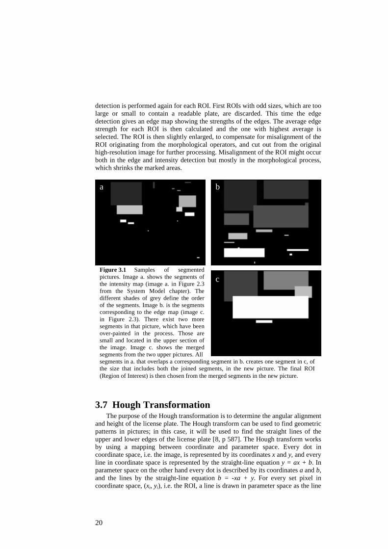
detection is performed again for each ROI. First ROIs with odd sizes, which are too large or small to contain a readable plate, are discarded. This time the edge detection gives an edge map showing the strengths of the edges. The average edge strength for each ROI is then calculated and the one with highest average is selected. The ROI is then slightly enlarged, to compensate for misalignment of the ROI originating from the morphological operators, and cut out from the original high-resolution image for further processing. Misalignment of the ROI might occur both in the edge and intensity detection but mostly in the morphological process, which shrinks the marked areas.

3.7 Hough Transformation The purpose of the Hough transformation is to determine the angular alignment

and height of the license plate. The Hough transform can be used to find geometric patterns in pictures; in this case, it will be used to find the straight lines of the upper and lower edges of the license plate [8, p 587]. The Hough transform works by using a mapping between coordinate and parameter space. Every dot in coordinate space, i.e. the image, is represented by its coordinates x and y, and every line in coordinate space is represented by the straight-line equation y = ax + b. In parameter space on the other hand every dot is described by its coordinates a and b, and the lines by the straight-line equation b = -xa + y. For every set pixel in coordinate space, (xi, yi), i.e. the ROI, a line is drawn in parameter space as the line

a b

c Figure 3.1 Samples of segmented pictures. Image a. shows the segments of the intensity map (image a. in Figure 2.3 from the System Model chapter). The different shades of grey define the order of the segments. Image b. is the segments corresponding to the edge map (image c. in Figure 2.3). There exist two more segments in that picture, which have been over-painted in the process. Those are small and located in the upper section of the image. Image c. shows the merged segments from the two upper pictures. All segments in a. that overlaps a corresponding segment in b. creates one segment in c, of the size that includes both the joined segments, in the new picture. The final ROI (Region of Interest) is then chosen from the merged segments in the new picture.

21

b = -xia + yi. When lines are drawn for all pixels, the point in parameter space, which most lines cross, is selected. Since the mapping between coordinate and parameter space is equal in both ways, the strongest dot in parameter space represent the strongest line in coordinate space. There is however a problem with the representation of a straight line as y = ax + b: When a line is close to the vertical the slope is approaching infinity. To cope with this problem the normal representation of a line can be used instead: x cos θ + y sin θ = ρ. With this representation of a line in coordinate space, the lines in parameter space are represented as sinusoidal curves. There are several advantages with this representation: the Hough space’s size is easier determinated, which is important for memory allocation matters when programming, and the angular resolution is equally distributed over the plot. The Hough transform with normal line representation is therefore used in this implementation. See Appendix A for further details and an example of a Hough plot.

The Hough transform requires reasonable input data, that is, in order to detect

lines from edges, edge detection is required so that every edge can be translated into lines. Before the edge detection is performed, the contrast of the picture is enhanced. The contrast enhancement algorithm in this stage is not really a contrast enhancer; it is more of a binarization method. The algorithm starts by calculating a threshold for each RGB colour that represents the 40 percent brightest pixels in the ROI. The threshold should represent the bright background part of the license plate, which at this stage is assumed to cover about 40 percent of the cut out ROI. For those pixels that have at least two colour values above the corresponding thresholds the output pixel will be set as bright, the rest is left unmarked, see Figure 3.2 b. The resulting binary picture, mostly showing just the plate background, is processed

Figure 3.2 Image a. shows the final ROI with the lines of the plate’s edge boarders from the Hough transform in green. Image b. is the contrast enhanced binary picture of the ROI. Image c. is the horizontal edge map of the contrast enhanced picture. Image d. is the final input to the Hough transform; it is the edge map after morphological erosion. The purpose of the Hough transform is to find the equations of the lines representing the upper and lower edge of the license plate. The input to the Hough transform needs to be a binary image with thin lines, which is most easily produced by an edge detection algorithm. The morphological erosion is used to get rid of unwanted edges like those from the characters.

a b

c d

22

with an edge detection algorithm. The edge detection in this step is similar to the earlier colour edge detection except this works vertically along the y-axis to find horizontal lines and the input is a single coloured binary image. It also only marks edges in the right direction, i.e. in the upper half of the picture, it only marks edges where it is dark above and bright below the edge and the opposite in the lower half. The edge detection also finds unwanted edges, like those from the characters, see Figure 3.2 c. These are however in rather small segments. These segments can be removed by using the morphological erosion again. The used structuring element now is one pixel high in y-direction and eleven pixels long in x-direction. It clears out all small edge segments and keeps only the long almost horizontal segments intact that are relevant for the Hough transform. The output of the edge detection is a binary picture where, in the optimal case, only the upper and lower edges of the licence plate are visible, see Figure 3.2 d.

The upper and lower halves of the ROI edge map are processed separately to make it easier to determine both of the equations for the upper and lower edge of the license plate. If the ROI would be processed in one piece, it would be harder to find the best lines. The parameters of the found equations for the lines are then equalized and compared. This gives a more accurate decision and a possibility to detect possible errors, such as if the difference of the angles are too large.

3.8 Affine Transformations The position and height of the license plate is now known. To be able to

perform the optical character recognition (OCR) the plate must be horizontally aligned and of uniform height. A set of steps to rotate and scale the plate will therefore be used. These are also called affine transformations. The first step is to rotate the picture. The rotation is performed with bilinear interpolation, earlier briefly described in Section 2.8. First, the size and position of the plate in the ROI are calculated using the line parameters from the Hough transform. A target image is allocated and for each output pixel the intensity level is calculated. The output image is filled row by row. The contribution to each destination pixel is calculated from the four closest source pixels. The contribution of each source pixel is calculated by taking the intensity times the covered area. Since no scaling is performed the whole area of both source and destination is set to one area unit. The calculation of the areas is simplified to give a fast but still reasonably accurate result, see Figure 3.3 and Equation (3.6) for how the rotated picture is determined. The motivation and description of the simplifications is as follows: The covered area is hard to calculate exactly, it is therefore estimated as the square from the corner of the source pixel to the corner of the destination pixel, instead of calculating the exact area of the quadrangle formed by the source and destination pixel, see Figure 3.3. In the example of Figure 3.3, it does not seem nontrivial to calculate the exact areas. Consider covering all the shapes and positions of the quadrangles when following the floating change from pixel to pixel. It will soon be troublesome to implement, and the complexity would drastically effect the computational time. See Figure 2.6 in the previous chapter for an example of how the intersections change in a larger grid. The size of the approximated squares is however easy to determine through the perpendicular distance from the beginning of the destination pixel, point A in Figure 3.3, to the point where the source pixels intersect, point B.

23

A perfect calculation of the covered areas would not be enough for an optimal output either. To be able to calculate the optimal output image more than just the covering pixels are needed in the input. For instance the more complex algorithm, bicubic interpolation, uses a neighbourhood of 4x4 pixels. Other methods found in sophisticated image manipulation programs use even more input pixels to feed higher complexity algorithms.

The horizontally aligned picture needs to be scaled to a specific height for the

OCR process to work optimally. To be able to scale the characters to the specific height the white background border above and below the symbols is removed. This is done by creating histograms over the joint row intensity, from which the beginning and end of the characters can be detected as the transition from the brighter borders to the darker characters. The resulting picture is then scaled using bilinear interpolation to the height of twenty pixels, regardless if it was larger or smaller from the beginning. The bilinear scaling is similar to the rotation but here the formed quadrangles in the intersections are at right angles which makes their

S1 Source pixel S2 A Destination pixel 0 d1 Reference points B d2 a d3 d4 θ 1 S3 S4 r s 0 b 1

( )

( )( ) ( )( ) ( )

( )

( ) ( )

( )6.3*cos,

*sin,

)1(*)1(*1,14

*1*,13

1**1,2

**,1

,sj

ri

bajiS

bajiS

bajiS

bajiS

srdθθ

==

−−++−+

−+=∑

Figure 3.3 The mathematical mapping from the red source pixels (S1,S2,S3,S4) to the blue destination pixel, d(r,s), when rotation using bilinear interpolation is performed by the angle θ. The coordinates (r,s) represent the pixel in the destination grid, (i,j) represents the source grid and is calculated from destination coordinates. The coordinates (a,b), (of the destination grid), of the intersection between the centre of the four source pixels (point B) is first determined. The approximated areas covering the destination pixel in form of the squares (d1, d2, d3, d4) can then easily be determined. The contribution from each source pixels is calculated as the fraction of the whole pixel that is covered.

24

sizes easy to determine exactly. The resulting image might still have flaws though. As has been explained earlier, more complex algorithms are required to create better output. The bilinear interpolation is just enough for this purpose though.

3.9 Optical Character Recognition The optical character recognition (OCR) algorithm works by comparing the

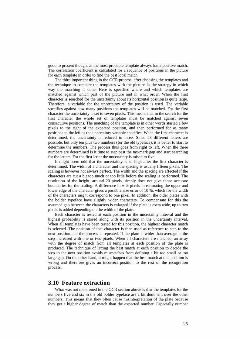
picture with predefined templates of the typeface used in the license plates of today. The templates are compared by calculating the normalized cross correlation. The templates were obtained from a typeface map from the Swedish Road Administration’s external plate manufacturer [13]. For the numbers four and five two different templates are used. Because a different, bolder, typeface was used during the years 1994 to 2001 [14], (it was a bold slightly modified Helvetica™ typeface). Those two templates were created by extracting them from a processed ROI of good quality. See Figure 3.4 for examples of how the templates look like. Before 1994 a third typeface was used, very similar to that of today, but with a few differing characters. No extra templates for these characters will be used since they are rather rare in traffic today.

The technique used to compare the picture with the templates is normalized cross correlation. The correlation is performed with a template and a section of the picture, both of size M x N pixels. A general form is presented in (3.7) below where f* denotes the complex conjugate. Images are however always real-valued why the conjugate can be ignored here. To get a uniform output with a comparable degree of match normalized cross correlation is used instead since the ordinary correlation described in (3.7), is sensitive to the amplitude of the image and the template.

( ) ( ) ( ) ( ) ( )∑∑−

=

−

=

∗ ++=1

0

1

0

7.3,,1

,,M

m

N

n

nymxhnmfMN

yxhyxf o

First, the pixel-values of the image and template are normalized to zero-mean

instead of being in the interval 0 to 255, i.e. the mean value is calculated and subtracted from each pixel. The normalized cross correlation is calculated with (3.8) where f and h now are zero-mean valued arrays of the image and template data.

( ) ( )

( ) ( )( )8.3

,,

,,

1

0

1

0

21

0

1

0

2

1

0

1

0

++=

∑∑∑∑

∑∑−

=

−

=

−

=

−

=

−

=

−

=

M

m

N

n

M

m

N

n

M

m

N

n

nmhnmf

nymxhnmfc

The resulting correlation coefficient, c, is in the interval -1 to 1. In the

application the result is scaled times one hundred and presented as a percentage. This is of course incorrect but the 0 % result would be the result of a correlation between the template and a randomized noise image. The negative result occurs only when there is more mismatch than randomness, e.g. c equal to -1 occurs only if the image is equal to the negative image of the template. The incorrect value is

25

good to present though, as the most probable template always has a positive match. The correlation coefficient is calculated for a sequence of positions in the picture for each template in order to find the best local match.

The third important thing in the OCR process, after choosing the templates and the technique to compare the templates with the picture, is the strategy in which way the matching is done. Here is specified where and which templates are matched against which part of the picture and in what order. When the first character is searched for the uncertainty about its horizontal position is quite large. Therefore, a variable for the uncertainty of the position is used. The variable specifies against how many positions the templates will be matched. For the first character the uncertainty is set to seven pixels. This means that in the search for the first character the whole set of templates must be matched against seven consecutive positions. The matching of the template is in other words started a few pixels to the right of the expected position, and then performed for as many positions to the left as the uncertainty variable specifies. When the first character is determined, the uncertainty is reduced to three. Since 23 different letters are possible, but only ten plus two numbers (for the old typeface), it is better to start to determine the numbers. The process thus goes from right to left. When the three numbers are determined is it time to step past the tax-mark gap and start searching for the letters. For the first letter the uncertainty is raised to five.

It might seem odd that the uncertainty is so high after the first character is determined. The width of a character and the spacing is usually fifteen pixels. The scaling is however not always perfect. The width and the spacing are affected if the characters are cut a bit too much or too little before the scaling is performed. The resolution of the height, around 20 pixels, simply does not give those accurate boundaries for the scaling. A difference in ± ½ pixels in estimating the upper and lower edge of the character gives a possible size error of 10 %, which for the width of the characters might correspond to one pixel. In addition, the older plates with the bolder typeface have slightly wider characters. To compensate for this the assumed gap between the characters is enlarged if the plate is extra wide, up to two pixels is added depending on the width of the plate.

Each character is tested at each position in the uncertainty interval and the highest probability is stored along with its position in the uncertainty interval. When all templates have been tested for this position, the highest character match is selected. The position of that character is then used as reference to step to the next position and the process is repeated. If the plate is wider than average is the step increased with one or two pixels. When all characters are matched, an array with the degree of match from all templates at each position of the plate is produced. The technique of letting the best match at each position to decide the step to the next position avoids mismatches from defining a bit too small or too large gap. On the other hand, it might happen that the best match at one position is wrong and therefore gives an incorrect position to the rest of the recognition process.

3.10 Feature extraction What was not mentioned in the OCR section above is that the templates for the

numbers five and six in the old bolder typeface are a bit dominant over the other numbers. This means that they often cause misinterpretation of the plate because they get a higher degree of match than the expected number. Especially number

26

eight often gets a lower match than five or six, although eight is actually correct. The degree of match between bold five and six are mostly very close. A reason to the better match of these templates might be that they were derived directly from a license plate processed by the program. For them, a good quality plate was processed in the program and the last, scaled and refined picture of the text was saved so that the numbers could be cut out and saved as templates. This make these templates a bit better fit to the characters than the other templates that were derived and scaled from a typeface-map.

To reduce the rate of failures, a simple version of feature extraction was

implemented. At first, the template for bold six is removed and not tested. Instead, the position of the best bold five is always stored separately. When all characters are matched against the current position, the picture is evaluated at the position where the bold five had its best match. The points of interest to evaluate for the character are the gaps in the upper right and lower left corners of the character 5, i.e. between the bar and the arc at the right side of the character and at the end of the lower arc, that if filled would form the ring of a 6. See Figure 3.4 where the areas are marked with a green frame. The mean value of the pixels in the assumed gaps are calculated and compared to the assumed mean value of a black/white bitmap, i.e. 127, to determine if the gap is filled or not. The probability of a bold six is then determined by increasing or reducing the degree of match of the template for the bold five depending on whether the gaps were filled or not. If the lower left gap is filled, the probability for a six is quite high, why its match is set

Figure 3.4 Some of templates used in the OCR process to read the text. The height is 20 pixels and the width is 11 pixels. For the numbers 4 and 5 are too different templates used, since they had a different shape during the years 1994 to 2001 when a bolder typeface were used. The bold template of the 6 is though not tested. Instead is the areas marked with green examined to see whether they are filled or not. This also prevents misdetection of an eight.

27

just above the probability of the five. If the upper right gap would be filled, neither a five nor a six is very probable, why their probabilities are reduced. This avoids misdetection of an eight. This technique to evaluate different fields of the picture to determine the characters could of course be used more extensively. Especially for the numbers it could probably be used for all matching since they are few and quite different. For the letters it could be harder since they have a larger variety in shape, which would narrow down the feature fields so much that it might require more work to figure out which letter is found than using the template matching.

3.11 Contrast enhancement In order for the correlation matching in the OCR process to produce as constant

results as possible a contrast enhancement is performed before the matching. The colours in the picture are mostly a bit blurred and the contrast is often low. The white colour is normally a light grey and the black is a darker shade of grey. With a uniform contrast, the result from different plates is more comparable. In the contrast enhancement, the colours are adjusted so that the darkest grey is ported to pure black and the brightest grey to clear white. All colours in-between are scaled so that they stretch out over the whole intensity scale. The thresholds, which define the intensity values that are mapped to maximum respectively minimum intensity of the picture, 255 or 0, are calculated from percentage values of the intensity distribution in the specific picture. In this implementation 20 percent is used for the dark threshold and 25 percent for the bright. The difference depends on the fact that the plate is assumed to contain larger white than black areas. The threshold is calculated from the defined percentage by counting the brightest and darkest pixels in a histogram, just like in the intensity binarization. See Figure 3.5 for an example of a processed image and a plot of the translation function. In Equation (3.9) the translation is described, where tmin is the low intensity threshold and tmax is the high intensity threshold represented as image intensity values [0, 255].

( )( )

( ) ( )( )

( )9.3

,,255

,,,

*255

,,0

,

max

maxminminmax

min

min

<

≤≤−

−<

=′

yxft

tyxfttt

tyxftyxf

yxf

The exact values of the percentage levels are not very important. It does not

make much difference if they would be 5 percentage points higher or lower. The selected values generally give a good result. If they would be too high, though, some pictures might be distorted. For instance, if both are set to 50 percent the picture will be mapped to a binary picture with values of either 0 or 255 and if the original picture only had 20 % dark areas, the least bright areas are mapped to black in order to fill up the quota of 50 percent. On the other hand, if the threshold would be too low the purpose of the enhancement is missed. The contrast enhancement is performed just before the OCR, after the scaling, in order to reduce the number of operations required, since the scaled picture normally has fewer pixels to manipulate.

28

3.12 Sequencing As is said before, the implementation cannot know from just one frame that a

correct license plate is found. The joint probability of a found plate’s characters varies between about 55 percent and up to 90 percent in the best cases. Incorrect plates, like plates where just one or two letters are misinterpreted might achieve a degree of match up to 65 percent or more. To support the decision of which license number is actually the correct one is the result from frame to frame sequenced. Since a car in front is likely to stay during several frames, the results from each frame can be combined. This is done by storing the probabilities for the most likely combinations in an array. The fact that the plate is found is also noted chronologically in a shift registry of length ten with the possibility of storing the hits for five different plates. Each time a new hit occurs, it is noted in the shift registry and the old hits are shifted back. If a previous found plate occurs in a latter frame the probability is updated with a forgetting factor of 80 percent. For those plates that does not occur is the probability decreased with a forgetting factor of 90 percent. The reason behind the different forgetting factors for hit or no hit is that the plate shift registry remembers the ten last interpreted frames so the probability is not supposed to be decreased too fast, but with a new hit, the new probability weight more compared to the stored value. If the frame-rate of the program gets too high, the shift-registry can be enlarged to cover more frames and the forgetting factor would need to be adjusted not to decrease the probabilities too fast. If the list is full and a new plate is found, it replaces the one with the lowest probability

255

0

0 tmin tmax 255 f(x,y)

f΄(x,y)

Figure 3.5 Schematic view over the mapping in the contrast enhancement from the original intensity values, f(x,y), at the x-axis to the enhanced scale in the new picture, y-axis, which uses the whole possible intensity range. The tmin and tmax represent the low and high intensity thresholds. All intensity values below tmin are mapped to zero, black, and all values above tmax are mapped to 255, white. The values in-between are scaled and stretched over the intensity range. To the right are two example pictures. The original above is black in the corners and clear white in the diagonal; the grey values are linearly fading. Below is the picture after processing with thresholds representing the 20 percent brightest and darkest pixels.

Original:

After processing with threshold 20 % for both dark and bright areas:

29

multiplied with the number of hits, regardless of whether the new plate’s probability is higher or not. With this method the accumulated probability of the found plates can be compared with how often they have occurred in order to give a good base for a correct decision of whether the interpreted plate is correct or not. The use of the forgetting factor also gives a chronological weight for each plate that assigns the last frames a higher significance. In Figure 3.6, an example of how the data stored in the sequencing arrays could look like after a few frames have been processed.

3.13 Design Parameters As has been mentioned previously in the different parts of the Implementation

chapter a set of design parameters are used. These parameters have the purpose of restricting the output of algorithms (e.g. define levels between possible noises and foreground, etc). The design parameters in the beginning adjust the ability to find ROIs in different images: These parameters are the scaling factor, defining the size of the initial work image, with influence on the computational time; the colour edge noise margin, defining the lowest accepted edge strength; the intensity threshold, defining the proportional intensity level; the morphological structuring element sizes. These parameters are important for the initial localization, where the approximate position and presence of a plate is determined. The effect of adjusting one parameter can be moderated by changing another one of them; it can therefore be hard to find the optimal setup. Different setups will have different abilities to detect the possible plate in different environments, e.g. if it is snowy or dark or if the plate is relatively small or large in the picture. The selected setup is the one that appears to be most general, i.e. it works for most of the samples.

These parameters cannot be optimized by mathematical methods since it is hard to define which results are incorrect and which are not. The parameters need to be balanced such that the plate is marked every time but not connected to other fields, which would make the ROI too large.

In the later processing part, the parameters are easier to determine since most of them only affects one step at a time. They can therefore be adjusted until an optimal result is reached for each individual function. Still it is hard to judge whether a parameter is optimal or not, maybe a failure is caused by the weakness of

Found plate Shift registry, frame n to n-9 n n-1 n-2 … … … … … … n-9 Σ hits Acc. P 1 ABC 123 1 1 1 1 1 5 57 % 2 DCE 456 1 1 23 % 3 FGH 789 1 1 1 3 83 % 4 FGH 289 1 1 67 % 5 - 0 0 % Figure 3.6 Example of how the sequencing is implemented. The plates are saved along with the probability and the time of occurrence. For each new interpreted frame the probabilities are decreased and the occurrence registry is shifted. The last found frame is noted in slot n, the previous hits in the n-1 and so on. By combining the data the most probable plate can be determined.

30

a later algorithm. Often the human eye is required to determine if the result is supposed to be good enough. These later design parameters are: the accepted size of a ROI after segmentation; the threshold of contrast enhancement before Hough transform; the limitations in angle in the Hough transform and the thresholds of the second contrast enhancement, just before OCR processing. In the following OCR process, several selected parameters are used, such as the expected step between characters and the uncertainty interval for each position. A change of these values affects the robustness contra computational time for the OCR process.

Last are the forgetting factors of the sequencing process and the length of its shift-registry. These parameters are mostly depending on the frame-rate and the required probability for a match to be considered correct.

To be able to evaluate the different parameter setups during the implementation a set of test images have been used. The test images are both from recorded sequences, as close to live detection as possible, and single shot images from the webcam and another higher quality camera. In addition, a set of images recorded indoors with the webcam filming a few high-resolution printed pictures. These last images might be the hardest to read since indoor light usually is more coloured than outdoor light, it is especially weak in the blue component.

31

Chapter 4 - Results This thesis has resulted in two implementations, one in Matlab® and one in

C++. Both implementations can recognise plates with a high probability of match. The C++ version can achieve a frame rate around 10 fps (tested on an 850 MHz 256 MB SDRAM laptop) depending on picture complexity and the relative size of the plate. As soon as the program finds out that it cannot possibly find a plate in the image, the processing of the next frame is started. The program will therefore be able to analyse more pictures when searching for not yet found plates or it can be restricted to a certain maximum frame-rate to spare computational resources for other applications.

This implementation has much higher recognition rate than the earlier version [6]. It can find smaller plates, like in Figure 4.1 where the distance between the green lines is 24 pixels. It can even recognise plates with text smaller than 20 pixels, which is equal to the height of the templates. A relatively small plate is of course more sensible to noise and even small misalignments in the detection might fail the detection since an error of one pixel in height is a relatively large error. This project’s implementation is very similar to one in [6], although all algorithms have been refined and developed. Parts of primarily the affine transformations have been more deeply altered. A part of the theory has been implemented as described, which was not the case before. The method of the Hough transform has been changed to make it more robust and it is now rarely the cause of a failure. The OCR method is somewhat better and significantly faster, although it might be a bit less robust since it assumes that the letters are perfectly narrowed in height and does not test the templates for different height positions. Otherwise, the implementation keeps much of the weaknesses from Schubert’s project. Bright areas such as snow or a bright white car might confuse the algorithm to find plates in other spots or so that it cannot narrow down the area of the plate. Colour doped images, which are very weak or too strong in one colour, causes the intensity or the colour edge detection to fail. Uneven lightning can make it difficult to distinguish between bright and dark areas, so that shadows can make a bright section look dark compared to a dark section that is illuminated.

A bottleneck in this project has been the camera. The now used web camera is sensitive to vibrations and fast changing targets since it has quite long shutter times. The optics used do not include auto-focus which would be useful. A good auto-focus makes large focus depth unnecessary, which allows for a larger aperture that can shorten the shutter time. A lower focus depth also reduces the background details, which might disturb the algorithm. A good feature reducing the effect of vibrations would be an image stabilizer. An infra-red camera along with an infra-red light source would give the best performance and weather independence [15]. Otherwise, the camera could be mounted in the grille of the car; the headlights would then give a good reflection in the license plate’s reflexive background.

32

Implementing in C++ gives powerful tools and fast programs. However, the

low-level hardware access has some drawbacks. Some misuse of the memory or indexing has made the implementation somewhat unstable. The program usually crashes after a while. Another remarkable note is that the C++ implementation is not always deterministic. The Matlab® implementation gives the same results for the same picture every time as it is supposed to, while it happens that the C++ version gives a different result from time to time, processing the same image. Usually it alters between a correct process and another one in some way incorrect, usually failed at the same erroneous state every time. The difference that has been noticed is that the Hough transform sometimes fails and does not give the correct alignment. But if the same picture is reprocessed again it does give the correct alignment. It also happens that it finds different ROIs from time to time. Generally the implementation has some problems with the memory handling which only makes it possible to analyse a few pictures at a time before the program needs to be restarted. Probably failed memory addressing and initialization cause the failures.

4.1 Future Work The implementation works quite well except for the reported software

problems. There is still room for improvement though. Here follows some things that can be improved.

Edge detection could be extended to feature a better colour filtering, i.e. it could be better to filter out colour-doped edges and accept a lower difference between the edge values from the different colour layers. For instance, the

Figure 4.1 Successful reading of a sample picture. This picture is harder than average to recognize since it contains a high level of details and bright areas of snow which might mislead the algorithms. On the other hand is the plate sharp which helps the OCR process. The low probability of match depends on the old bolder typeface of this plate which differs a bit from the templates used.

33

maximum difference between the strongest layer edge-magnitude and the lowest could be restricted. Experimental implementations of these techniques have been tested, but did not give a generally better result, i.e. it improved recognition of some pictures but failed in other previously recognised ones. Another method could be to produce a black/white image optimized to highlight the plate and then perform edge and intensity detection on it instead of the colour image. White areas have the properties of a very high intensity in all colour layers and a very low difference between the colour layers. By for instance selecting the lowest intensity value of each pixel and subtracting the difference between the highest and lowest colour values are intense white areas highlighted, intense coloured areas like rear lights are suppressed to almost black. This method requires though rather good images, the colouring needs to be even and no single colour can be too weak. The computing time of the transform to black/white would though be saved by the lower complexity of black/white images. In addition, the contrast enhancement just before the Hough transform might also be improved by better colour filtering.

The RGB colour representation used in this implementation is very simple to understand and manage in computer processing. It is though not optimized for describing license plates; plates are optimized to be readable by the human eye. By using the colour representation of HSV (hue, saturation, value) or HSI (hue, saturation, intensity) might an advantage be gained in finding the black/white features of the plates [16, 17]. Hue describes the main colour, saturation is the amount of whiteness in the colour and intensity is the brightness. The RGB representation makes it very hard to extend the implementation to recognise plates using other background than white, for instance taxi plates and diplomatic cars.

The segment merging function utilizes the segment output images and can not yet create ROIs from all the overlapping input segments. As in the sample pictures, Figure 2.4 and 3.1, where there exists small segments surrounded by large segments, but which are still not connected to the large ones and therefore supposed to be independent segments. Both the small and the large segments have corresponding segments in the other picture and should therefore yield two different but mostly overlapping ROIs, which is not the case in the current implementation. This issue is corrected for in the segmenting function by double-checking against the input picture if neighbouring segments exist and not against the supportive output image. To change the merging algorithm in a simple way is however not possible and it needs in large parts to be rewritten to support surrounded segments. It can already handle segments that partly overlap.

The implementation has a frame-rate that in some environments is much higher than what is necessary. The complexity of some algorithms could therefore be raised to gain in recognition rate. The selection of the ROI could be improved by letting more combinations of segments to be examined. The implementation could maybe even let several ROIs be examined parallel until the OCR processing is started.

The method of finding the plate in the ROI by searching for the upper and lower edge is robust. It is however harder to narrow down the exact location of the plate, especially if the ROI is much larger than the plate. The OCR method is sensitive to misalignment of the characters and to difference in size. This part is therefore clearly improvable.

34

35

References [1] http://www.vision.cmit.csiro.au/expertise/ocr/ Optical Character Recognition. Australia. 2006-04-07 [2] http://www.cclondon.com/ London Congestion Charging. 2006-05-10 [3] http://www.stockholmsforsoket.se/ “The Stockholm Trials” congestion charging. 2006-05-10 [4] http://www.speedcheck.co.uk/ SPECS speed cameras, United Kingdom. 2006-05-10 [5] http://www.singaporegateway.com/optasia/ IMPS, system for car park management, tolls etc in Singapore and Malaysia. 2006-05-10 [6] Schubert, Robin, “License plate recognition on a real-time testbed”, Royal Institute of Technology, Stockholm, November 2005, IR-SB-EX-0524 [7] http://www.vv.se/templates/page3____3771.aspx Sök fordons- och ägaruppgifter. Vägverket. Search for vehicle and owner information, Swedish Road Administration. 2006-05-31. (Only in Swedish) [8] Gonzalez, Rafael C. and Woods, Richard E. “Digital Image Processing” Prentice Hall, Inc. 2nd Edition. 2002. [9] http://www.vv.se/filer/1196/Registreringsskyltar.pdf Swedish license plates from the Swedish Road Administration. 2006-10-24 [10] Li Huiping and D. Doermann. “Superresolution-Based Enhancement of Text in Digital Video” In 15th International Conference on Pattern Recognition, 2000. Proceedings., pages: 847-850 vol.1, 2000 [11] Farsiua, S. et al. “Robust Shift and Add Approach to Super-Resolution” In Applications of Digital Image Processing XXVI. vol. 5203, 2003, pages: 121-130 [12] Yuntao Cui, Qian Huang. “Extracting characters of license plates from video sequences.” Machine Vision and Applications, Vol. 10, April 1998, pages: 308-320, Springer-Verlag. ISSN: 0932-8092 [13] http://www.absmc.se/ AB Scandinavian Motorcenter. The company that manufactures the Swedish license plates on behalf of the Swedish Road Administration. [14] http://sv.wikipedia.org/wiki/Registreringsskyltar_i_Sverige License plates in Sweden. 2006-06-07. (Only in Swedish)

36

[15] http://www.appian-tech.com/products/I-Star.htm Appian Technology PLC, ALPR solutions and cameras. 2006-05-18. [16] Beatriz Díaz Acosta, “Experiments in Image Segmentation for Automatic US License Plate Recognition”, Virginia Polytechnic Institute and State University, 2004-06-18, URN: etd-07022004-132444. [17] Chang, S. et al. “Automatic License Plate Recognition” In IEEE Transactions on Intelligent Transportation Systems. vol. 5, no. 1, March 2004, pages: 42-53.

37

Appendix A

A.1 The Hough Transform The Hough transform is used to find straight lines in images and it can also be

used to find more advanced patterns like circles. The following text will describe the method of finding lines. The transform works by taking advantage of the way a line is represented. If the normal representation of a line is used: x*cos θ + y*sin θ = ρ, where θ is the angle of the line, ρ is the intersection with the y-axis and x and y are the coordinates for the points on the line. A direct mapping can be defined between a line’s parameters in the picture, also called parameter space, and the coordinates of a spot in Hough space, and vice versa. To detect lines in the picture an empty Hough plot is first created. Then, for every set pixel in the picture, a sinusoid curve is added to the Hough plot. If the plot is oriented as the plot in figure A.1, the curve is plotted such that for every value on the horizontal axis (representing an angle of a possible line) the value on vertical axis is set to be the value of the y-axis intersection of that possible line. This gives a sine curve for every pixel. For every set of two pixels, there is an intersection of their sine-curves in Hough space representing the line between them. When a curve for each pixel is added to the Hough space, the strongest lines can be found by looking for local maxima. With the coordinates of the maxima given, the equations for the lines can be determined by the reversed mapping. To improve performance or to create useful input an edge detection algorithm might be used first.

Node A

Node B

Line B

Line A

Angle of line, θ

Inte

rse

ctio

n of

y-a

xis,

ρ

Figure A.1 The left picture is an intensity map with two strong lines, A and B. To the right is a Hough plot of the picture where sinus-curves have been added for all marked (white) pixels in the picture. For lines in the picture, several pixels will generate sinus-curves that intersect at the same point for angle and value of y-axis intersection. Therefore, the strongest lines in the picture can be found by looking for the strongest values in the plot. The nodes marked in the Hough plot corresponds to the lines A and B in the picture. The coordinates of that spot can be directly mapped to the equation of the line. Since the sinus curve is periodical, corresponding spots can be seen just in the beginning of the plot, representing the reversed angle.

Hough plot: