Page 1
Low default modelling: a comparison of techniques based on a
real Brazilian corporate portfolio.
Guilherme Fernandes and Carlos A. Rocha *
April 8th
, 2011
Abstract: Over the past decade modelling expected loss has been a subject of interest to
financial institutions. As defined by BIS Basel II accord, the probability of default (PD)
is a parameter of the expected loss of a portfolio. The methodologies for modelling the
PD on a retail credit portfolio are well explored [1997: Hand and Henley]. However,
financial institutions must deal with low default situations, for instance corporate
portfolio. Plutto&Tasche [2006] have shown a conservative methodology for estimating
the PD based on a previous defined rating. This paper explores and compares some
techniques to develop a PD rating on a low default scenario. First we revisited some
models that would fit in this situation, such as classical logistic regression, Bayesian
logistic regression and limited logistic regression. Artificial oversampling via SMOTE
[2002: Chawla et al.] was conducted to result on a balanced data and the state dependent
correction [1989: McCullagh and Nelder] was then applied to extract bias from
estimators. Those four techniques were used in the analysis of a real dataset based on
corporate companies from Brazil. There were a total of 1.327 enterprises of which 50
defaulted on a 12 month outcome window. Comparisons evaluated relied on ROC
curve, Gini coefficient and Kolmogorov-Smirnov statistics. Those three statistics were
analyzed after a bootstrap simulation. As results, limited logistic regression presented
slightly higher K-S statistics throughout the simulation. This model returned the highest
K-S statistics over 50% of the re-samplings. However, when Gini coefficient is
analyzed classical logistic regression performed better. Over 42% of all re-samplings
pointed towards this model as the best fit.
Key-words: Low default models, Bayesian logistic regression, state dependent
correction, limited logistic regression, corporate statistical modelling.
*Serasa Experian, Al. Quinimuras, 187, São Paulo, SP – Brazil.
E-mail: [email protected] , [email protected]
Page 2
1. Introduction
Banks and financial institutions play important role in the economy as money
multiplier. This implies to accelerated economic increase and creates a virtuous cycle of
borrowing, generating wealth, payment with interest and borrowing again. Nevertheless,
there is a systematic risk inherent to credit. The credit risk, better known due to BIS
Basel Accord, has been a subject of great interest to financial system entities.
Since the loss of a portfolio can be considered a random variable conditional to
some risk factors, it became a major research field to model those factors. As a random
variable, one can calculate the expectation of the loss function of a portfolio. The
expected loss (EL) can be understood as the most likely cost to a credit portfolio and as
so it sets the inferior limit to a safe reserve. As defined in BIS New Basel Accord
(2001), the expected loss (EL) can be expressed as the product of the probability of
default (PD), exposure at default (EAD) and loss given default (LGD).
There are many academic researches over those three factors, especially PD.
When it comes to a retail portfolio with plenty of default and observations, all usual
methods for modelling can be applied and evaluated. However, financial institutions
also deal with low default portfolios (LDP). The Basel Accord does not set a rule to
classify a portfolio as a LDP, however FSA [1] suggests three broad categories. One of
those is set as “no or insufficient data (…) available (…) to derive PD estimates”.
There are a numbered of papers that deals with PD bounds estimation, such as
Pluto [2], however most of them are based on previous rating grade. This paper explores
and compares some techniques to estimate a statistical model and an input to the rating
grade.
First we discuss the well-known classical logistic regression, one of the main
approaches to model PD of a non-LDP. Cramer [3] introduced a different technique, the
limited logistic regression, which is based on adding a parameter to the logistic model to
set an upper bound to the output probability. A Bayesian logistic regression was also
considered here using a non informative priori.
Since low event is the main source of concerning when modelling a LDP, an
oversampling technique could set a possible direction. Among many computational
algorithms to inflate the number of defaults, Chawla et al. [4] suggested the SMOTE
Page 3
technique, a method that artificially creates new default observations based on the pre-
existing ones. According to McCullagh [5] a logistic regression estimated from this new
dataset would present biased parameters, however the state-dependent correction solves
the bias.
A Brazilian corporate credit portfolio was the basis of comparison to the present
paper. A total of 1,327 companies were observed during a ten-year window and a one-
year outcome time horizon to determine default. This portfolio presented a 3.7% default
rate and 50 defaulted companies were detected. In spite of a rather high default rate, the
number of defaults causes a modelling difficulty.
As comparison measures we used the area under the ROC (AUROC) curve [6]
and the Kolmogorov-Smirnov statistic (KS) [7]. Uncertainty arises due to the low
number of defaults in the sample and hence, a bootstrap simulation [8] was run to
minimize this problem. The results of the simulation showed that Bayesian logistic
regression presented a high level of performance with a lower bootstrap variance.
2. Methodologies
On credit risk models one of the most commonly used techniques is logistic
regression because of its properties, such as, parameters that are easily interpreted and
linear combination of risk factors. As Hand and Henley [9] pointed out: “(…) there is
no overall „best‟ method”. Hence, our comparison is not an ultimate list for modelling
techniques that should be compared. Discriminant analysis, neural networks, time-
varying models and, why not, linear regression are only some plausible alternatives [9].
We cover primarily logistic regression like models.
a. Classical logistic regression
Logistic regression is part of a widely general family of models known as
generalized linear models [5]. The model is stated from a dichotomous response
variable. Let Yi be the observation of the default event over the outcome window where:
Page 4
{
(1)
The probability modelled is a non-linear link function to a linear combination of
the risk drivers (vector of endogenous variables xi‟). Therefore, the logistic regression is
described as follows.
[ ] ( )
( ) (2)
The equation (2) means that the probability of a credit lender honours the debt is
estimated conditionally on the endogenous variables (xi‟). The main reason of logistic
regression being chosen as the credit risk scoring methodology is the direct
interpretation of the parameters. In logistic regression exp(β) represents the odds ratio.
Also the direct probability of an event is more tangible idea to non-literates on statistical
modelling.
Risk factors effect over the probability of default (PD) is expressed by the β
parameters vector. The estimation method of these parameters in logistic regression is
the maximum likelihood estimation (MLE). The likelihood function is given by the joint
distribution of all observations conditioned to Xi variables, stated in (3).
( ) ∏ ( ) ∏ ( ( ))
( ( ))
(3)
The maximum of ( ) is also maximum of ( ) ( ( )).
( ) ∑ * (
( )) ( ) (
( ))+
(4)
After solving the system obtained from ( )
, the estimates are the
MLE. Hypothesis testing of those estimates is based on Wald’s statistic [10] and is
given by:
[
( )]
(5)
The W statistic has normal distribution under H0, so the regular test is applied.
The logistic regression perhaps, may present low quality estimates for the
vector [3]. Cramer [3] suggests a slight modification for that model adding one
Page 5
parameter. This model was called limited logistic regression and is stated in the
following section.
b. Limited logistic regression
The limited logistic regression presents an extra parameter that sets an upper
bound for the probability of default and is stated in (6).
[ ] ( )
( ) (6)
In equation (6) the Yi, xi‟ and have similar meaning as in classical logistic
regression, however is the additional parameter that bounds the probability (
). The probability distribution of Yi is once again Binomial( ( )) and, therefore, the
likelihood function is similar to (3). The log-likelihood function is presented in (7) and
the only difference from (4) is because of .
( ) ∑ * (
( )) ( ) (
( ))+
(7)
From equation (4) the system of equations ( )
is found and it leads to
a non-linear system on the parameters. To estimate both parameters and , an
iterative optimization method is needed and Newton-Raphson’s algorithm [11] was run.
The hypothesis testing for is also based on Wald’s statistics.
c. Bayesian logistic regression
In statistical modelling, Bayesian inference incorporates the level of uncertainty
towards the parameters. This uncertainty is reduced after data information is taken into
account. The prior distribution holds the uncertainty before data and the posterior
distribution is the parameters marginal distribution after data incorporation. The
equation (8) presents the relationship stated.
( ) ( ) ( )
∫ ( ) ( ) (8)
Page 6
Where ( ) is the prior distribution of the parameter of interest, ( ) is the
likelihood function and represents the data information added and, at last, ( ) is the
posterior distribution.
Equation (8) is based on the Bayes theorem and to solve this equation a series of
simulation methods have been developed, one of the most widely used is based on
Gibbs sampling [11]. Simulation diagnosis is needed and some useful tools are:
1. Time series graphics for simulation steps to showing stability and low
variability,
2. Autocorrelation graphics [12] to assure non-correlation,
3. Geweke test [13] as convergence criteria.
The three diagnosis tools have been used in this paper.
d. Artificial oversampling via SMOTE
As pointed by Cramér [3], most techniques loose performance and result on low
quality estimates modelling a rare event. Chawla et al [4] suggest a computational
method for artificially creating new observations and balance both events, default and
non default.
The synthetic minority oversampling technique, or SMOTE as it was called,
randomly creates observations from existing defaults. The randomness is embedded in
the selection of two existing observations and again to simulate a synthetic point inner
to the hypercube they define. The steps to simulate new observations are described as
follows.
Illustration 1 represents a data set with two possible covariates, X1 and X2, and
the observed individuals with those characteristics. Notice that black dots stands for
default and white dots for non default. The first step is to select only the minority class,
Illustration 2.
Page 7
Illustration 1 Illustration 2
The next step is represented in Illustration 3, where a pair of observations is
randomly sampled. Their coordinates define a semi-plan and within it the synthetic
observation is, once again randomly, created. Illustration 4 shows the results of the
SMOTE simulation after several iterations.
Illustration 3 Illustration 4
Based on the new data set at Illustration 4 the model is developed. Although it
solves the problem of low data, the lack of real proportion of default / non default
introduces bias to the estimates. This problem is called state-dependent sample and
McCullagh and Nelder [5] present a solution.
e. State-dependent correction
The SMOTE method increases the minority class to a reasonable rate of
default/non default. However, as mentioned, it introduces a bias to the parameters
estimation and the problem is called state-dependent sample. The equation (9) states
proposition in mathematical terms.
( ) ( ) (9)
X1
X2
X1
X2
X1
X2
X1
X2
Page 8
Where Yi = 1 means default state for the ith
observation and S is the sample for
modelling. After the SMOTE is run the resulting data set is a state-dependent sample
and the bias of estimation process is known. Equation (10) sets log-likelihood function
under state-dependent sample.
( ( )) ∑ ( (( ) ) (10)
Where wi is the weight of the observation given by (
) (
) ( ),
with is the real proportion of defaults and is the sample proportion of defaults.
Both covariates vector and parameters vector are represented as in (3). Although
the estimates are still biased, the correction presented in McCullagh and Nelder [5]
solves this problem. Equation (11) state the bias.
( ) ( ) ( ) (11)
Where ( [ ( ) ] [( ( ⁄ )) ( ⁄ )])) ; with W is the
weight diagonal matrix, 1is a ones-vector and is the vector of estimated
probabilities for each observation. At last, the estimated parameters are obtained
from ( ). According to King and Zeng [18] is consistent for all i ,
in other words, every parameters but the intercept. They suggest a simple
correction that is elucidated in Equation (12).
*(
) (
)+ (12)
f. Performance measures
In order to compare and evaluate the four methods for modelling LDP, two main
measures were calculated: Gini coefficient and Kolmogorov-Smirnov statistic. The first
one was introduced by Corrado Gini [14] and originally used to measure inequality.
Commonly found in sociology to quantify wealth distribution, can also scale
discriminatory power of a PD model.
Gini’s coefficient is based on the Lorenz curve and it is calculated as a ratio of
areas on Illustration 5. The line that delimits areas A and B is the Lorenz curve and it is
Page 9
plotted from the pairs of accumulated defaulted and non-defaulted observations for all
possible cut-offs on the ordered PD estimates.
Illustration 5
Gini’s coefficient is calculated as ( )⁄ . The higher is G, the better
discriminatory power the model presents. Therefore, if G = 1 then the model perfectly
separates defaulted and non-defaulted. Notice that Gini’s coefficient has a one-to-one
link to the area under the ROC curve.
The second performance measure used is the Kolmogorov-Smirnov statistic
[15], from now on KS. It is a non parametric statistic meant to compare empirical
distributions and is used to compare default and non-default PD estimates distributions.
Equation (13) presents Dn,n‟ as the KS statistic.
[ ( ) ( ) ] (13)
Notice that the KS statistic measures the maximum distance between empirical
accumulated distributions of both groups, while Gini’s coefficient evaluates the whole
curve. Although they usually points out to the same direction, the conclusions might be
divergent.
g. Bootstrap simulation
In 1979 Bradley Efron [8] introduced the bootstrap simulation. The algorithm
has been of great value in various statistical analysis situations, from estimation of
Acumulated non-defaulted
Acum
ula
ted
defa
ulted
A
B
Page 10
parameters to model validation. Here we resort to bootstrap as part of the model
evaluation analysis. Since performance measures are susceptible to high variability in
LDP, bootstrap has been a tool to bypass possible over-fitting besides measuring impact
of a few defaults.
The bootstrap algorithm is based on resampling the data set with reposition
criteria k times. Every resample must have the same size as the original data.
Bootstrapping relies on independent observations and perhaps it is a reasonable
assumption even in LDP.
At last we obtained several KS(k) statistics and Gini(k) coefficients. The analysis
is based on the distribution of both measures and the model with the highest average
statistic on both maybe chosen if variability is smaller.
3. Results
a. Data description
The data set used was a real corporate portfolio, which implies in company
revenues over US$ 130 million (R$ 200 million). The modelling period is from 2003
through 2008, resulting on 1.327 different companies. Default definition is based on
market default for a one-year performance window, such criterions resulted in 50
defaults over time.
Although a 3.76% default rate is not a rare event situation, the fifty defaulters
brings up the problem of a LDP. The main difficulty is found in estimating parameters
avoiding over fitting risk.
The period used for modelling process is punctuated by several characteristics,
most of them unique in Brazilian history. During this period the index [16] of variation
wages on a year-over-year basis, raised from -15% in 2003 to +4%. Credit over gross
national product ratio [16] also grew from 22% in 2003 to 36% in 2008. Nevertheless
credit delinquency [16] ranged from 3.5% to 5.0%. The propitious economic
environment induces a low default scenario and the challenge for modelling process is
established. The Graph 1 shows this scenario.
Page 11
Graph 1: Default rate over months
It is valuable to notice from Graph 1 that in the majority of months no defaults
were observed. Even the moving average (bold line) presents sharp edges. The crisis
period is observed after the fourth quarter of 2007 and here note that the default status is
evaluated under a twelve months window.
b. Approaches comparison
The analysis of the data set previously described began with a default correlation
overview through several covariates. Information value (IV) [17] was primarily
calculated for all eligible variables. IV is based on Weight of Evidence (WoE) adjusted
by cases percent in each class. Equation (14) presents the calculation need to obtain IV
for a continuous form. Equation (15) presents IV for discrete form.
∫( ) (
) (14)
∑( ) (15)
Where WoE = ln(DistDefault/DistNonDefault). A variable with higher IV has
better discriminating power. Notice that IVD is not sensible for default rate inversion,
thus a closer analysis is needed towards discrete variables.
0%
1%
2%
3%
4%
5%
6%
7%
0
10
20
30
40
50
60
set/
03
no
v/0
3
jan
/04
mar
/04
mai
/04
jul/
04
set/
04
no
v/0
4
jan
/05
mar
/05
mai
/05
jul/
05
set/
05
no
v/0
5
jan
/06
mar
/06
mai
/06
jul/
06
set/
06
no
v/0
6
jan
/07
mar
/07
mai
/07
jul/
07
set/
07
no
v/0
7
jan
/08
mar
/08
mai
/08
jul/
08
Non defaulted Defaulted Default Rate Moving Average Average Default Rate
Page 12
Variables available in the data set refer to information about: credit demand,
historical bureau delinquency, short-long indebtedness, suppliers’ info and balance
sheet accounts. After data cleaning, the 120 variables available for modelling only 54
presented IV higher than 0.3.
Multicollinearity is an issue that may lead to over-fitting and biased parameters
estimation. As a mean to solve it, each pair of covariates with Spearman correlation
coefficient higher than 0.5 were submitted to an IV comparison and the lowest one
excluded from the model. There were 29 variables after such analysis and none of them
had IV lower than 0.5.
The first model estimated was classical logistic regression and a sort of stepwise
procedure was conducted. The priority of variables tried on the model was defined by
the Information Value of each. The final model included the following variables: V1)
total negative bureau statements included over the past 30 days, V2) ratio of short term
debt over current assets, V3) number of banking past due contracts, V4) days since last
negative statement paid, V5) maximum of negative statements active at the same time,
V6) total enquiries over the past 15 days, and at last V7) number of negative statement
paid over the past 6 months. The Table 1 presents estimates and p-value for each
parameter.
Table 1: Parameters estimates and their hypothesis tests
The last columns of Table 1 also compares the discriminatory power of each
variable in the model by evaluating the PD change when varying each input values in a
ceteris paribus view held equal to their mean. Here notice that variable V7 (Negative
statement paid over the past 6 months) presents the highest difference in PD, followed
Standard Wald
Error Chi-Square Min Max Odds
Intercept -3.6228 0.5241 47.7843 <.0001
Ratio of short term debt over current assets higher than 25 0.8451 0.3132 7.2799 0.007 0.015 0.033 2.284
Total of negative bureau statements included over the
past 30 days higher than 81.0701 0.4509 5.6311 0.0176 0.018 0.051 2.818
Number of banking past due contracts (Max of 4) 0.2638 0.0954 7.6552 0.0057 0.015 0.042 2.794
Days since last negative statement paid (Max of 200 days) -
square root tranformation-0.1744 0.0503 12.0377 0.0005 0.058 0.005 11.154
Maximum of negative statements active at the same time
(Max of 120) - square root transformation0.1713 0.0571 8.9922 0.0027 0.010 0.060 6.200
Total number of enquiries over the past 15 days (Max of
50)0.0320 0.012 7.1265 0.0076 0.011 0.050 4.755
Total number of negative statement paid over the past 6
months (max of 45) - square root transformation-0.4637 0.128 13.1203 0.0003 0.064 0.003 21.069
PD RangeParameter Estimate P-value
Page 13
by V4 (Days since last negative statement was paid) and V5 (Maximum number of
statements active at the same time). The variable V6 (Total enquiries over the past 15
days) adds a meaningful discriminatory power increment.
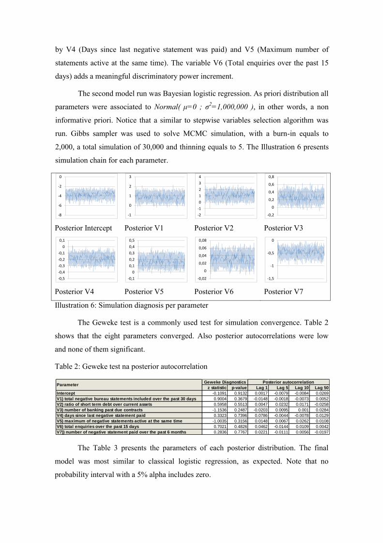
The second model run was Bayesian logistic regression. As priori distribution all
parameters were associated to Normal( μ=0 ; σ2=1,000,000 ), in other words, a non
informative priori. Notice that a similar to stepwise variables selection algorithm was
run. Gibbs sampler was used to solve MCMC simulation, with a burn-in equals to
2,000, a total simulation of 30,000 and thinning equals to 5. The Illustration 6 presents
simulation chain for each parameter.
Posterior Intercept
Posterior V1
Posterior V2
Posterior V3
Posterior V4
Posterior V5
Posterior V6
Posterior V7
Illustration 6: Simulation diagnosis per parameter
The Geweke test is a commonly used test for simulation convergence. Table 2
shows that the eight parameters converged. Also posterior autocorrelations were low
and none of them significant.
Table 2: Geweke test na posterior autocorrelation
The Table 3 presents the parameters of each posterior distribution. The final
model was most similar to classical logistic regression, as expected. Note that no
probability interval with a 5% alpha includes zero.
-8
-6
-4
-2
0
-1
0
1
2
3
-2
-1
0
1
2
3
4
-0,2
0
0,2
0,4
0,6
0,8
-0,5
-0,4
-0,3
-0,2
-0,1
0
0,1
-0,1
0
0,1
0,2
0,3
0,4
0,5
-0,02
0
0,02
0,04
0,06
0,08
-1,5
-1
-0,5
0
z statistic p-value Lag 1 Lag 5 Lag 10 Lag 50
Intercept -0.1091 0.9132 0.0017 -0.0079 -0.0084 0.0269
V1) total negative bureau statements included over the past 30 days 0.9004 0.3679 -0.0148 -0.0018 -0.0073 0.0052
V2) ratio of short term debt over current assets 0.5958 0.5513 0.0047 0.0232 0.0171 -0.0258
V3) number of banking past due contracts -1.1536 0.2487 -0.0203 0.0095 0.001 0.0284
V4) days since last negative statement paid 0.3323 0.7396 0.0786 -0.0044 -0.0078 0.0129
V5) maximum of negative statements active at the same time -1.0035 0.3156 0.0148 0.0067 0.0262 0.0108
V6) total enquiries over the past 15 days 0.7021 0.4826 0.0462 -0.0144 0.0109 0.0042
V7)) number of negative statement paid over the past 6 months 0.2836 0.7767 0.0221 -0.0111 0.0056 -0.0197
Geweke Diagnostics Posterior autocorrelationParameter
Page 14
Table 3: Posterior distributions and equal-tail interval
The last columns in Table 3 compare the discriminatory power of each variable
in the Bayesian model. The PD change was evaluated by varying its input values while
others variables are held fixed and equal to each mean. Once again, variable V7
(Negative statement paid over the past 6 months) presents the highest difference in PD,
followed by V4 (Days since last negative statement was paid) and V5 (Maximum
number of statements active at the same time). Variable V6 (Enquiries over the past 15
days) presented one of the widest PD range. The parameters found are slightly different
from the ones estimated in classical logistic regression, although it raised the odds in
PD range.
The third methodology presented was limited logistic regression. In order to
estimate the parameters of this model, the log-likelihood function (7) was defined and
maximized using the Newton-Raphson algorithm [11]. Table 4 presents estimated
parameters and p-value (H0: β=0). Once again a sort of stepwise selection method was
applied and the same variables entered the model. Note that w here represents the upper
bound of the PD.
Standard
Deviation Min Max Odds
Intercept -3.6974 0.5298 -4.7738 -2.7080
Ratio of short term debt over current assets higher than 25 0.8651 0.3178 0.2553 1.5130 0.013 0.031 2.333
Total of negative bureau statements included over the past
30 days higher than 81.0901 0.4585 0.1821 1.9817 0.016 0.047 2.882
Number of banking past due contracts (Max of 4) 0.2686 0.0975 0.0791 0.4596 0.014 0.039 2.853
Days since last negative statement paid (Max of 200 days) -
square root tranformation-0.1793 0.0515 -0.2839 -0.0814 0.054 0.005 11.992
Maximum of negative statements active at the same time
(Max of 120) - square root transformation0.1727 0.0583 0.0557 0.2837 0.009 0.055 6.323
Total number of enquiries over the past 15 days (Max of 50) 0.0324 0.0120 0.0090 0.0564 0.009 0.046 4.866
Total number of negative statement paid over the past 6
months (max of 45) - square root transformation-0.4718 0.1312 -0.7332 -0.2214 0.059 0.003 22.343
PD RangeMean
Equal-Tail Interval
(alpha 5%)Parameter
Page 15
Table 4: Parameters estimates and hypothesis tests
The last columns in Table 4 compare the discriminatory power of each variable
in the limited logistic model. The PD change was evaluated by varying its input values
while others variables are held fixed and equal to each mean. Once more variable V7
(Negative statement paid over the past 6 months) presents the highest difference in PD,
followed by V4 (Days since last negative statement was paid) and V5 (Maximum
number of statements active at the same time). Also the limited logistic regression
raised the odds in PD range considerably.
At last, the SMOTE oversampling method for artificial data creation was set to
generate a database of 1,277 non-defaulted (all original ones) and 430 defaulted (50
original observations and 380 synthetic data). The logistic regression estimation occurs
under the weighted maximum likelihood function where the weights are presented in
Equation (16).
{
(16)
The Table 5 presents parameters estimates, their hypothesis test with weight
matrix and the state-dependent corrected parameters after bias calculation (11). Notice
that the correction of the intercept has a slightly different formula (12). Most parameters
were almost bias-free prior to state-dependent correction.
Min Max Odds
w 0.146 <0.0001
Ratio of short term debt over current assets higher than
250.969 0.008 0.015 0.033 2.262
Total of negative bureau statements included over the
past 30 days higher than 82.127 0.018 0.017 0.077 4.502
Number of banking past due contracts (Max of 4) 0.303 0.006 0.015 0.041 2.695
Days since last negative statement paid (Max of 200
days) - square root tranformation-0.334 0.001 0.084 0.002 48.346
Maximum of negative statements active at the same
time (Max of 120) - square root transformation0.336 0.003 0.005 0.088 16.365
Total number of enquiries over the past 15 days (Max of
50)0.014 0.008 0.016 0.028 1.779
Total number of negative statement paid over the past 6
months (max of 45) - square root transformation-0.862 0.001 0.089 0.001 128.881
PD RangeParameter Mean P-value
Page 16
Table 5: Parameters
The last columns in Table 5 compare the discriminatory power of each variable
in the limited logistic model. Once more, the PD change was evaluated by varying its
input values while others variables are held fixed and equal to each mean. Variable V7
(Negative statement paid over the past 6 months) presents the highest difference in PD,
followed closely by V4 (Days since last negative statement was paid) and furthermore
by V5 (Maximum number of statements active at the same time).
In order to compare the four methodologies a bootstrap simulation was run with
10,000 re-samples. Gini coefficient and KS statistic were calculated in each re-sample.
At last, two boxplots completed the comparison, on for each performance measure.
Graph 2: KS comparison
Min Max Odds
Intercept -0.9824 <.0001 -2.1523 -3.1347
Ratio of short term debt over current assets higher than 25 1.0975 <.0001 0.0000 1.0975 0.015 0.042 2.912
Total of negative bureau statements included over the past
30 days higher than 80.7722 0.0001 0.0012 0.7710 0.020 0.042 2.113
Number of banking past due contracts (Max of 4) 0.2789 <.0001 0.0002 0.2787 0.016 0.048 2.951
Days since last negative statement paid (Max of 200 days) -
square root tranformation-0.1772 <.0001 -0.0001 -0.1771 0.064 0.006 11.526
Maximum of negative statements active at the same time
(Max of 120) - square root transformation0.1421 <.0001 0.0001 0.1420 0.012 0.054 4.538
Total number of negative statement paid over the past 6
months (max of 45) - square root transformation-0.3782 <.0001 -0.0002 -0.3780 0.056 0.005 11.976
Total number of distinct companies that enquiried over the
past 15 days was higher than 350.7395 <.0001 0.0000 0.7395 0.020 0.041 2.050
PD Range
Estimate P-value BiasCorrected
estimateParameter
35,00
40,00
45,00
50,00
55,00
60,00
65,00
Classical Model Limited Logistic Bayesian Model State Dependent
Boxplot for KS statistic
Page 17
Graph 3: Gini coefficient Comparison
At overall view to Graphs 2 and 3 suggests that state-dependent correction after
SMOTE oversampling presents lower median Gini coefficient and median KS statistic.
The limited logistic regression presents the highest median KS statistic, however Gini
coefficient is four points lower.
When comparing the median Gini and median KS for both Bayesian and
classical logistic regression they presented similar results. Nevertheless, KS
interquartile range was, by far, larger in the classical model. Apparently the MCMC
simulation provides a higher robustness to the posterior parameters in the Bayesian
model.
The default rate assortment along score quantiles also was found. Graph 4 shows
that when one splits the score into 15 ranges of equal proportion of observations, the
default rate in each class (bold line) rises in a rather assorted direction. The inverted
accumulated default rate (dashed line) presents a monotonically non-decreasing pattern.
40,00
45,00
50,00
55,00
60,00
65,00
70,00
75,00
Classical Model Limited Logistic Bayesian Model State Dependent
Boxplot for Gini coefficient
Page 18
Graph 4: Default rate assortment
4. Conclusion
Banks were always interested in risk measurement and after Basel accord its
importance increased substantially. Among risk parameters, PD occupies a central role.
In a retail portfolio no greater difficulties have been found to estimate PD models,
however when it comes to low default portfolios estimation issues arise. Pluto and
Tasche [2] introduced one of the most used methods for assessing PD. Nevertheless,
their method starts from a pre-existing rating grade. This paper illustrated and compared
four alternatives to obtain such a rating model.
Classical logistic regression, limited logistic regression, Bayesian logistic
regression and oversampling technique combined with state-dependent correction were
compared in a Brazilian LDP. The estimated parameters in final models were alike and
slight differences in estimates were found. However, after a bootstrap simulation of
Gini coefficient and KS statistic, the Bayesian model presented high performance with
lower variance.
Although limited logistic regression presented the best KS statistic, the top
performance was not repeated in Gini coefficient. SMOTE combined with state-
dependent correction provided a lower performance in both measures. Classical logistic
regression presented similar performance to Bayesian model, but the KS statistic
variance in bootstrap simulation was high and first quartile of classical model was
further lower than in the Bayesian model.
0,0% 0,0%1,1% 1,1% 1,1%
2,2%
0,0%
3,4%2,3%
3,4% 3,4%
1,1%
9,1%7,9%
20,5%
3,8% 4,0% 4,3% 4,6% 4,9% 5,3% 5,7%6,4% 6,8%
7,5%8,4%
9,6%
12,5%
14,1%
20,5%
0
10
20
30
40
50
60
70
80
90
100
0%
5%
10%
15%
20%
25%
0,2
9%
0,4
2%
0,5
6%
0,7
1%
0,8
5%
1,0
5%
1,3
2%
1,6
1%
2,0
0%
2,4
8%
3,0
8%
4,1
7%
5,6
5%
8,4
7%
20
,32
%
# o
bse
rvat
ion
s
De
fau
lt r
ate
Mean point per score class
Bayesian model - Default rate assortment
# observations Default rate Inverted accumulated default rate
Page 19
Another important aspect in PD modelling is the assortment of default rate
throughout score ranges. Bayesian model presented a rather increasing trend as score
would rise. For those reasons Bayesian logistic regression was considered the best
option for this situation.
An informative priori Bayesian model would be a subject of further studies.
Specialist information and external bureau odds ratio may be a way of assessing an
informative priori distribution.
5. Reference
[1] Financial Services Authority (2005): “Expert Group paper on Low Default
Portfolios.”, Credit Risk Standing Group, August 2005.
[2] Pluto, K. and Tasche, D. (2006) “Estimating Probabilities of Default for Low
Default Portfolios.”, Risk, April 2006.
[3] Cramer, S. (2004): “Scoring bank loans that may go wrong: a case study.” Statistica
Neerlandia, 2004, Vol. 58, n. 3.
[4] Chawla, N.; Bowyer, K.; Hall, L. and Kegelmeyer, W. (2002): “SMOTE: Synthetic
Minority Over-sampling Technique.”, Journal of Artificial Intelligence Research, June
2002.
[5] McCullagh, P. and Nelder, J.A. (1989): Generalized Linear Model, 2nd
Edition,
Chapman & Hall / CRC.
[6] Green, D.M. and Swets, J.M. (1966): Signal detection theory and psychophysics.
New York: John Wiley and Sons Inc.
[7] Smirnov, N.V. (1948): "Tables for estimating the goodness of fit of empirical
distributions", Annals of Mathematical Statistic, v. 19.
[8] Efron, B. (1979). "Bootstrap Methods: Another Look at the Jackknife". The Annals
of Statistics v. 7 (1).
[9] Hand, D.J. and Henley, W.E. (1997): “Statistical Classification Methods in
Consumer Credit Scoring: A Review”. Journal of the Royal Statistical Society – Series
A, Vol. 160, Issue 3.
Page 20
[10] Hosmer, W.D. and Lemeshow, S. (2000): Applied Logistic Regression. New York:
Wiley.
[11] Gelman, A.; Carlin, J.; Stern, H. and Rubin, D. (1995): Bayesian data analysis.
London: Chapman and Hall.
[12] Box, G.; Jenkins, G. and Reinsel, G. (1994): Time Series Analysis: Forecasting and
Control. Upper Saddle River, NJ: Prentice–Hall.
[13] Geweke, J. (1992), “Evaluating the Accuracy of Sampling-Based Approaches to
Calculating Posterior Moments” in J. M. Bernardo, J. O. Berger, A. P. Dawiv, and A. F.
M. Smith, eds., Bayesian Statistics, Vol. 4, Oxford, UK: Clarendon Press.
[14] Gini, C. (1912): “Variabilità e mutabilità” C. Cuppini, Bologna, 156 pages.
Reprinted in Memorie di metodologica statistica (Ed. Pizetti E, Salvemini, T). Rome:
Libreria Eredi Virgilio Veschi (1955).
[15] Corder, G.W. and Foreman, D.I. (2009).Nonparametric Statistics for Non-
Statisticians: A Step-by-Step Approach Wiley
[16] Central Bank of Brazil series.
[17] Hababou, M.; Cheng, Y. and Falk, R. (2006): “Variables selection in credit card
industry”, North East Sas User Group – Nesug 2006, Philadelphia, US.
[18] Moraes, D. (2008): Credit Card Fraud Models. Master degree dissertation, Federal
University of Sao Carlos, Brazil.