Low Energy Adaptive Routing Hierarchy Based on ...

INTERNATIONAL JOURNAL ON SMART SENSING AND INTELLIGENT SYSTEMS VOL. 6, NO. 2, APRIL 2013

523

Low Energy Adaptive Routing Hierarchy Based on Differential Evolution

Xiangyuan Yin [1,2], *Zhihao Ling [1,3] and Liping Guan

Shanghai, China, Email:

[2]

1 School of Information Science and Engineering, East China University of Science and Technology

yxy2000yxy@ zwu.edu.cn

2 Zhejiang Wanli University, Ningbo, China, Email: [email protected]

3 Key Laboratory of Advanced Control and Optimization for Chemical ProcessMinistry of Education,

China, Email: [email protected]

*Corresponding author: Zhihao Ling

Submitted: Dec. 17, 2012 Accepted: mar. 27, 2013 Published: Apr. 10, 2013

Abstract- In recent years, wireless sensor network (WSN) is a rapidly evolving technological platform

with tremendous and novel applications. Many routing protocols have been specially designed for WSN

because the sensor nodes are typically battery-power. To prolong the network lifetime, power

management and energy-efficient routing techniques become necessary. In large scale wireless sensor

networks, hierarchical routing has the advantage of providing scalable and resource efficient solutions.

To find an efficient way to decrease energy consumption and improve network lifetime, this paper

proposes a centralized routing called Low-Energy Adaptive routing Hierarchy Based on Differential

Evolution (LEACH-DE). Simulation results show that the proposed routing protocol outperforms other

well known protocols including LEACH and LEACH-C in the aspects of reducing overall energy

consumption and improving network lifetime.

Index terms: Routing Algorithm, Differential Evolution, Cluster Head, LEACH-DE.

brought to you by COREView metadata, citation and similar papers at core.ac.uk

provided by Exeley Inc.

https://core.ac.uk/display/226931451?utm_source=pdf&utm_medium=banner&utm_campaign=pdf-decoration-v1

mailto:[email protected]�

mailto:[email protected]�

http://www.showxiu.com/fan_yi/In_the_aspect_of/�

Xiangyuan Yin, Zhihao Ling, and Liping Guan, Low Energy Adaptive Routing Hierarchy Based on Differential Evolution

524

I. INTRODUCTION

Recently researches on wireless sensor network (WSN) have rapidly grown and new techniques

have been developed for efficient transmission. Typically, a WSN consists of hundreds or

thousands of low cost sensor nodes scattered among danger environments and difficult-to-reach

terrains and networked together for collaboratively gathering data from an area of interest [1].

Each sensor node always has an embedded processor, a wireless module, a non replaceable

energy and some on-board sensors. Once deployed, sensor node has a limited power supply since

it only rely on batteries so that sensor node may fail as a result of energy depletion,

communication link errors, and so on [2]. At the same time, where many applications in WSN

require many-to-one traffic pattern, multihop forwarding may lead to energy imbalance because

all the traffic must be routed through the nodes near the data sink, thus creating a hot spot around

the data sink. Nodes in hot spot are required to forward high amount of data and always die at a

very early stage. Therefore, energy-efficient routing algorithms, protocols and deployment

strategies play key roles in minimizing transmission energy and prolonging network lifetime.

According to the network structure, routing algorithm in WSN can be divided into flat-based

routing algorithm, hierarchical-based routing algorithm. Some flat routing algorithm including

SPIN (Sensor Protocols for Information via Negotiation), DD (Directed Diffusion), and MCFA

(Minimum Cost Forwarding Algorithm) are proposed in early years [3, 4, 5, 6]. Hierarchical

routing is an efficient way to lower energy consumption within a cluster and to decrease the

number of messages transmitted to the sink node by performing data aggregation. In hierarchical

networks, higher energy nodes can be used to process and send the information while low energy

nodes can be used to perform the sensing task [7, 8]. Hierarchical routing is typically separated

into two phases that one phase is used for selecting cluster heads and the other phase is used for

routing and transferring actual data. By clustering, nodes are organized into small groups called

clusters. Each cluster has a cluster head (CH) and some non cluster head (non CH) nodes.

Compared with flat routing, clustering protocol can provide obvious superiority with respect to

energy conservation by facilitating localized control and reducing the volume of inter-node

communication [9]. Some of routing protocols in this group are: LEACH [10], PEGASIS, TEEN

and APTEEN. LEACH [11] is one of the most studied and referred protocols, which is

considered as the ground work for other hierarchical routing.


525

The paper proposes another clustering-based routing protocol called LEACH based on

differential evolution (LEACH-DE), which utilizes differential evolution algorithm to find cluster

heads and set up clusters. The motivation behind the LEACH-DE is that selecting the most

appropriate CH for a group of sensor nodes by minimizing the distance between CHs and non CH

nodes. The rest of the paper is organized as follows. In the next section, the classical hierarchical

routing protocols are overviewed with detailed discussions. Section 3 exhibits the structure of

LEACH-DE and network model, respectively. In section 4, we evaluate the performance of

LEACH-DE and compare the performance of LEACH-DE with that of other hierarchical routing

algorithms. Finally, section 5 concludes the paper and highlights some future work directions.

II. RELATED WORK

As previously mentioned, cluster-based routing protocol is to efficiently maintain the energy

consumption of sensor nodes by selecting appropriate cluster heads (CHs) and by performing

data aggregation in order to decrease the number of transmitted messages to the sink. Among the

hierarchical routing protocols in wireless sensor networks, LEACH [11, 12] is a well-known

routing protocol, which is used as the ground work for several researches.

2.1 LEACH

In LEACH, time is partitioned into fixed intervals with equal length, which is called topology

update interval or round. Each round is generally separated into the setup phase and the steady

state phase. During the setup phase, each node decides whither or not to become a CH for the

current round based on a predetermined fraction of nodes and the threshold value, T(s). The

threshold value is calculated by Eq. (1).

∉

∈⋅−=

Gsif

Gsifprp

p

sT

0

))/1mod((1)( (1)

Where p = k/N is the percentage of cluster head accounted for all nodes, r is the number of

election rounds, )/1mod( pr ⋅ refers to the number of nodes elected in the previous r-1 round of

cycle, and G is a set of non elected nodes in the previous r-1 round. In steady-state phase, nodes

can begin sensing and transmitting data to the cluster heads during their allocated transmission


526

slot. To reduce energy dissipation, the radio of non cluster head node is immediately turned off

after transmitting data. Once the cluster head receivers all the data, it performs data aggregation

before sending data to the base station (BS).

2.2 LEACH-C

In [12, 13], an extension to LEACH, LEACH-C is proposed. In order to ensure energy load is

evenly distributed among all the nodes, the sink node in LEACH-C finds clusters using the

simulated annealing to solve the NP-hard problem of finding k optimal clusters. During the setup

phase, each sensor node transmits information about its location and remaining energy to the BS.

The BS computes the average node energy, and the nodes whose energy level is above this

average value may be selected as CH in the current round. This algorithm uses simulated

annealing algorithm for selecting CH, which can minimize the total sum of distances between CH

nodes and non CH nodes in order to decrease the total power consumption of the WSN. The

overall performance of LEACH-C is better than LEACH since LEACH-DE moves duty of

cluster formation to the base station (BS), predetermines the optimal number of cluster, selects

the appropriate nodes as CH.

2.3 TL-LEACH

As a single-hop routing algorithm for WSN, the CH collects and aggregates data from nodes and

transmits the information to BS directly in LEACH. According to the radio energy dissipation

model, both the free space ( 2d power loss) channel models and the multipath fading ( 4d power

loss) channel models are used. Which channel model is used depends on the distance between the

transmitter and receiver. To transmit a l -bit message for a distance d , the radio expends the

amount of energy is described by Eq. (2).

≥∗∗+<∗∗+

=0

40

2

),(dddllEdddllE

dlEmpelec

fselec

εε

(2)

The electronics energy Eelec

fsε

depends on factors such as the digital coding, modulation, filtering,

and spreading of the signal, whereas the amplifier energy or mpε depends on the distance to the

receiver and the acceptable bit-error rate. The short distance is defined as mp

fsd εε

=0 . In

LEACH, each CH directly communicates with sink no matter the distance between CH and BS is


527

far or near. CH will consume lots of energy for transmit data if the distance is greater the

threshold 0d . Losci et al. [13] proposed a two-level hierarchy for LEACH (TL-LEACH) which

uses one of CH that lie between the CH and the BS as a relay station. This algorithm utilizes two

levels of cluster heads (primary and secondary). The primary cluster head in each cluster

communicates with their secondaries, and the corresponding secondaries communicate with the

sensor nodes in their sub-cluster. The algorithm can effectively prolong the lifetime of battery-

powered sensor nodes because transmit distance is reduced. LEACH-type protocols have

received significant developed recently, but some shortcoming of those protocols should be

attention.

As mentioned above, LEACH and TL-LEACH [14] are completely distributed and requires no

any global knowledge of the network. LEACH-C is an improved scheme of LEACH in which a

centralized algorithm at BS makes cluster formation, which needs GPS or other location-tracking

method in order to gain the position of sensor nodes. The core algorithm of LEACH-C is

simulated annealing (SA) which is a traditional generic probabilistic metaheuristic for the global

optimization with slowly convergence [15]. SA is a randomized gradient descent algorithm,

which permits uphill moves with some probability so that it can escape local minima. But SA is

not universal and its performance is dependable on some requirements which make SA converge

very slowly in most the global optimization, these requirements include that the initial

temperature is high enough, the temperature is cooled slowly enough, etc. These protocols do not

guarantee that appropriate nodes are select as CHs [16].

2.4 Swarm intelligence

Swarm intelligence (SI) [17] is developed from the imitations which are learned from the social

behaviors of insects and animals, for example: Differential Evolution (DE) [18], ant colony

optimization (ACO) [19], particle swarm optimization (PSO) [20], and the like. SI has found

practical applications in areas such as intelligent control, robotics, and wireless sensor network.

Researchers have successfully used SI techniques to address many challenges in WSN. Among

these SI techniques, DE is successfully applied to a remarkable number of NP-hard problems

because of search through vast spaces of possible solutions [21]. Clustering a network to

minimize the total energy dissipation is an NP-hard problem. For the total number of sensor

nodes in WSN is N, a sensor node is either elected as CH or non CH in each solution so that there

http://en.wikipedia.org/wiki/Metaheuristic�

http://en.wikipedia.org/wiki/Global_optimization�





528

are 12 −N different combination of solutions for the WSN [11]. So DE can been applied for

solving NP-hard problem. Storn and Price(1995) firstly proposed the differential evolution (DE)

which has become one of the most frequently used evolutionary algorithms for solving the global

optimization problems [22]. Compared with most evolutionary algorithms, DE is based on a

mutation operator, which adds an amount obtained by the different of two randomly chosen

individuals of the current population. The algorithm of DE is shown as follow:

1. generate an initial population DXXXXP iN ∈= },,...,,{ 21

2. repeat

3. For i:=1 to N do

4. Generate a new trial vector iY

5. if )()( ii XfYf < , then y replace iX

6. end if

7. generate new population ,P

8. end for

9. until the termination condition is achieved

The next generation )1( +tXi

is determined by the following three operations: mutation,

crossover and selection.

Mutation

Mutation strategies were previously proposed in [23], the most popular mutation strategy called

DE/rand/1/bin. Mutate individual of DE/rand/1/bin is generated according to the following

equation:

)]()([)()(321

tXtXftXtY iimii −+=

Ni ,,2,1 = is the individual’s index of population; 1i

X ,2i

X ,3i

X are randomly chosen vectors

from the set { }pNi XX ,,

1 ; pN is the population size; the mutation factor mf is a parameter in

[ ]1,0 , which controls the amplification of the difference from two individuals so as to avoid

search stagnation [24]. The other frequently referenced mutation strategies are listed below:

(1) “DE/Best/1”: )]()([)()(21

tXtXftXtY iimbesti −+=


529

(2) “DE/RandToBest/1”: )]()([)]()([)()(211 tXtXftXtXftXtY iimibestmii −+−+=

(3) “DE/Best/2”: )]()([)]()([)()(4321 1 tXtXftXtXftXtY iimiimbesti −+−+=

(4) “DE/Rand/2”: )]()([)]()([)()(54321 1 tXtXftXtXftXtY iimiimii −+−+=

(5) “DE/RandToBest/2”:

)]()([)]()([)]()([)()(4321 21 tXtXftXtXftXtXftXtY iimiimibestmii −+−+−+=

Crossover

Crossover operations are applied to increase the potential diversity to the population which use

binomial crossover scheme. The binomial crossover scheme constructs the trial vector by

taking , in a random manner, elements either from the mutant vector )(tX i or from the current

element )(tYi , as is described in Eq.(3).

=<=

=otherwisetX

IjorCRrandiftYtY j

ij

j

i

i

i )()1,0()(

)(

(3)

iI is a randomly selected index from },2,1{ n which ensures that at least one component is take

from the mutant vector )(tYi .The parameter CR (crossover rate) is a user-specified constant

within the range [0,1] which controls the number of components inherited from the mutant vector

and influences the convergence speed.

Selection

When all N trial points )(tYi

have been generated, selection operation is applied. We must decide

which individual between )(tXi

and )(tYi

should survive in the next generation )1( +tX

i, the

selection operator is described as follows:

>

=+otherwisetX

tXftYfiftYtX

i

iiii )(

))(())(()()1(

In addition the DE dynamically tracks current searches with its unique memory capability to

adjust its search strategy. DE has comparatively strong global convergence capability and

robustness and no need with the help from information about the characteristics of problems [25].


530

III. THE PROPOSED ALGORITHM LEACH-DE

To increase the lifetime of WSN, this paper proposed an energy efficient routing algorithm, this

is, LEACH based on DE algorithm (LEACH-DE). LEACH-DE is a specially designed routing

algorithm for WSN with the sink being an essential component with complex computational

abilities, thus the other nodes being very simple and cost effective. LEACH-DE works in rounds

as LEACH and each round consists of two main phases, the setup phase and the steady state

phase. During the setup phase, the selection of the cluster-head follows the similar criteria as

LEACH, but the algorithm of selection cluster-head in LEACH-DE is differential evolution

algorithm. The setup phase is subdivided into selection of cluster-head phase and formation of

cluster phase. The flowcharts of selecting cluster-head phase and formatting of cluster phase are

respectively shown in Figure 1(a) and Figure 1(b).

no

yes

Get the position of all nodes

Confirm the best number of CH

Initialize population of DE

operate mutation , crossover and

selection

Create the new generate of population

Create the new generate of population

Compute the fitness of distance

Meet constraint condition?

Find CH and cluster formation

Node I isCluster-head

Wait for join-request message

Announce cluster-head status

Creat TDMA schedule and send to cluster members

Send join-request message

Wait for cluster-head announcements

Wait for schedule from cluster-head

Steady-state operation

Figure 1(a). Selection of cluster-head phase Figure 1(b). Formation of clustering phase.

In this paper, the simulation assumed that there are 100 sensor nodes and one sink which are

randomly dispersed in a two-dimensional square field and sensor network has the following

properties:

There are only one sink in the network, which is static and no energy constraints.

Sensor nodes are non-rechargeable, have equal initial energy and always have data to send.

Packets loss due to factors other than the energy exhausting of node not exist or is ignorable

Nodes are aware of their location.


531

Communication from each node can be used by the radio energy dissipation model which

presented in Eq.(2).

Each node can directly communicate with the sink.

The WSN in the paper can be modeled as an undirected graph ),( EVG = where, V is the node

set and E is an edge set. There are the total of N sensor nodes are initially distributed randomly

in a two-dimensional field A， S is a set of N and Nk ≤ a positive integer. A k -clustering of

S into k subsets kSSS 21 , .Each iS is called a cluster which has one CH and some non CH

nodes. Non CH node in the cluster sends data to its CH only. The goal of the clustering algorithm

attempts to minimize the amount of energy for the non cluster head nodes to transmit their data to

the cluster head, by minimize the total sum of distance between all the non CH nodes and the

closest cluster head. The clustering problem can be considered as k-mean problem which is NP-

Hard. So in the cluster iS , the number of the non CH nodes is N and the distance between CH

and the non CH node j can be computed as given below.

22 )()(),( jijii yyxxjSCHdis −+−= (4)

Where, ),( ii yx and ),( jj yx represent the position of the CH and the node j . According of the

goal of the clustering problem, we should find a set VS ∈ , with KS = so as to

∑∑= =

=K

i

N

ji jSCHdisVSt

1 1),(min),(cosmin (5)

Subject to : 100,0 ≤≤ ii yx

The objective function can be solved by different heuristics algorithms. For such routing

protocols, the number of clusters within the network is highly affecting to the network lifetime

and the energy consumption. The optimal number of clusters is very important. Numerical

simulate tests showed that if the number of clusters are not equal to an optimal number, the total

consumed energy of the sensor network per round is increased significantly. In [12], optk which is

the optimum number of CHs within the network can be calculated by Eq. (6).

2.2 toBSmp

fsopt d

MNkεε

π=

（6）

Where toBSd is the distance from the CH to the BS.

The pseudo-code of the LEACH-DE algorithm is given below:

http://dict.youdao.com/search?q=calculate&keyfrom=E2Ctranslation�


532

---------------------------------------------------------------------

Definitions:

D: Dimensions of problem, D=2 in the paper

NP：population size

CR：crossover rate

F: scale factor

MNG: maximum number of generations which is a termination criterion.

new_index(i,:): The vector index with the lowest cost

Cost(S,V): The distance of CHs and non CHs

MNG: Maximum number of generations specified

FM_popold: Initial population

FM_ui: New population

F_weigh: The weighted vector difference

Maxbound: The upper bound value, Maxbound=100

Minbound: The lower bound value, Minbound=0

find_min_dist: Distance calculation function

step 1: Generate one sink and 100 homogeneous sensor nodes, which are shown in Fig.2.

step 2: Initialize the values of D and key parameters (NP, CR, F and MNG).

step 3: Randomly generate population. The population consists of NP competitions, and

each competition has optk CH nodes in the study.

For i=1 : NP

{For j=1 to optk

InitCutou(i,j)=random number

{ x1(i,j)=x(1, InitCutou(i,j));

y1(i,j)=y(1,InitCutou(i,j)) }

Generate population: FM_popold=[x1,y1]}

step 4: Evaluate the Cost(S,V) of each vector according to Eq. (5), find out CHs.


533

For i=1 to NP

{Cost(S,V)=find_min_dist(x1(i,:),y1(i,:),size1,x2,y2,size2);

Find out new_index(i,:)}

Where x1(i,:), y1(i,:), size1 are the x- , y- coordinate and the number of CH respectively,

and x2,y2,size2 are the x-, y- coordinate and the number of non CH respectively.

step 5: Perform mutation, crossover, selection and evaluation of the objective function

Cost(S,V).

While (gen< MNG)

{ for i=1 to NP

Perform mutation for each target vector.

When the mutation strategy is DE/rand/1,

FM_ui = FM_pm3 + F_weight*(FM_pm1 - FM_pm2);（The other mutation strategies

can be seen in section 2）

Perform Binomial crossover.

If ( CRrand ≤)1,0( or iIj = )

FM_ui = FM_popold.*FM_mpo + FM_ui.*FM_mui;

Check whether new vector are within the bounds. If not, the new vector must be

restricted within the bounds.

if (FM_ui(k,j) > FVr_maxbound)

FM_ui(k,j) = maxbound + rand*( origin(k,j) - maxbound);

if (FM_ui(k,j) < FVr_minbound)

FM_ui(k,j) = minbound + rand*( origin(k,j) - minbound);}

Find out new CHs.

Through the above process, the five CHs calculated may be not sensor nodes. The

“new” CHs can be found out according to the minimal distance.

Cost(S,V)=find_min_dist(x1new(i,:),y1new(i,:),size1,x2,y2,size2)

Find out new_index(i,:)


534

Perform selection.

For i=1 to NP

{ if (costnew(i) <cost(i) )

new )(tX i= )(ˆ tYi

;

otherwise new )(tX i= )(tX i

}

Print the results and continue.

Print the results;

If (gen< MNG)

gen=gen+1

Jump to step 5.

---------------------------------------------------------------------

IV. PERFORMANCE EVALUATION

4.1 Comparison between different strategies of DE

The clustering of WSN is optimization problem in the sense that energy consumption is

distributed over all sensor nodes and the energy consumption of whole network is minimal. To

evaluate the performance of LEACH-DE, simulation experiments were tested with various

experimental scenarios which were simulated in Matlab. The experiments were carried out in two

major phases. In the first phase, the paper evaluates the different strategies of DE and determines

the most appropriate parameters and strategy. In the second phase, the paper compares the

performance of LEACH-DE with that of LEACH and LEACH-C in terms of the convergence

value and total remain energy in the network.

In the study, five strategies of DE are used to solve the Eq. (5). They are DE/Best/1,

DE/RandToBest/1, DE/Best/2, DE/Rand/2 and DE/RandToBest/2 which are given in section 2.

The result of the strategies are studied to find the most strategy and the most parameters for

minimize the total sum of distance between all the non CH and CH according to the Eq. (5). In

the simulation experiments, we set the parameters of WSN as [7], that is, N=100, M=100m,

75m< toBSd <185m, pJfs 10=ε , pJmp 0013.0=ε , and optk =5.


535

The simulated WSN consists of one sink which located at the origin of coordinate system and

100 homogeneous sensor nodes randomly deployed within the sensing field from (0,0) to

(100,100), which be shown in Figure 2.

Figure 2. Sensor nodes deployed in WSN

Figure 3 shows the example of dynamic cluster formation. All nodes marked with a given symbol

belong to the same cluster, and CHs are marked with a circle.

Figure 3. Example of dynamic cluster formation


536

In every generation, five nodes are selected as CHs which can be conceded as a seed in order to

minimize ),(cos VSt . Normally, NP (population size) should be about 5~10 times the number of

parameters in a vector, in the study, NP=10. Maximum number of generations (MNG) is the

number of iterations that the algorithm will run. For easy problems, one may start with 100

generations. Then, if necessary, the value can get increased until the algorithm can not improve

result. In the paper, MNG is 1000.

In order to validating the effectiveness of the LEACH-DE and determined the appropriate

parameter, 500 independent runs were performed in the paper. The performance of DE depends

on key parameters, namely, mutation strategy, CR, F, and NP. By choosing the key parameters

(mutation strategy, NP, CR, and F) appropriately, the problem of premature convergence can be

avoided to a large extent. The paper applies the simulation with the following parameter settings:

NP=10, MNG =1000. CR is varied from 0.1 to 1 at step of 0.1 and F is varied from 0.1 to 1 at

step of 0.1, which can be seen in the Table 1.

Table 1 Parameter setting of LEACH-DE NP MNG CR F Strategy

LEACH-DE 10 1000 (0.1~1) step=0.1

(0.1~1) step=0.1 1~5

Now, in order to study the effect of F and CR on various strategies, the criterion considered is

“converge to the minimum value”. In LEACH-DE, mf (scale factor) influences the diversity of

the set of mutant vectors and CR（crossover rate） controls the fraction of parameter values

copied from the mutant vector. In the study, the best combination of CR and mf are chosen by

trial and error. CR was varied from 0.1 to 1 at step of 0.1, mf was varied from 0.1 to 1 at step of

0.1，which leading to 100 combinations of CR and mf for the DE algorithm.

When the LEACH-DE algorithm is executed with five strategies for all the above combinations,

the results of numerical simulation show that the globe minimum value for Eq. (5) is 1635.5

which is likely to converge to the true global optimum. Every strategy can converge to the

minimum value（1635.5） but the numbers of converging the minimum is different. DE/Rand/2

Parameter

Algorithm


537

and DE/RandToBest/2 can reach the globe minimum more than 20 times and have the lower

average convergence value which means the two strategies have more superior performance than

other strategies. Table 1 shows the final convergence situation for different strategies.

Table 2 Final convergence situation for different strategies

Convergence value

Strategy

Average final

convergence value

Numbers of converging

to minimum

DE/Best/1

(Strategy 1) 1685.8 8

DE/RandToBest/1

(Strategy 2) 1690 3

DE/Best/2

(Strategy 3) 1732.4 5

DE/Rand/2

(Strategy 4) 1669 20

DE/RandToBest/2

(Strategy 5) 1646.4 21

The results in the Table 2 record the final convergence situation for different strategies. From the

Table 2, it is observed that if for a given certain condition, by using DE/best/1… (Strategy

numbers 1 to 5) the global minimum can be achieved in a certain generations. Results in the

Table 2 clearly illustrate that the strategy 4 and strategy 5 are significantly better than the other

strategies in that the strategy 4 and strategy 5 can converge to minimum value above twenty

times against other strategies can not.

Once good strategies are chosen, the next step is to study the effect of the key parameters of DE

to find the best combinations of F and CR for good strategies. So the study selects DE/Rand/2

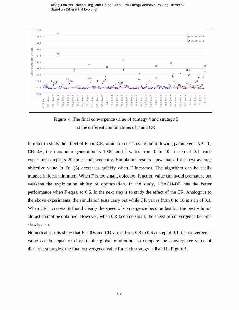
and DE/RandToBest/2 (strategy 4 and strategy 5) as the core strategies of LEACH-DE. Figure 4

shows the situation of final convergence value of strategy 4 and strategy 5 at the different

combinations of F and CR.


538

1620

1640

1660

1680

1700

1720

1740

1760

1780

1800

1820

F=0.

1 R=

0.1

F=0.

1 R=

0.4

F=0.

1 R=

0.7

F=0.

1 R=

10

F=0.

2 R=

0.3

F=0.

2 R=

0.6

F=0.

2 R=

0.9

F=0.

3 R=

0.2

F=0.

3 R=

0.5

F=0.

3 R=

0.8

F=0.

4 R=

0.1

F=0.

4 R=

0.4

F=0.

4 R=

0.7

F=0.

4 R=

1

F=0.

5 R=

0.3

F=0.

5 R=

0.6

F=0.

5 R=

0.9

F=0.

6 R=

0.2

F=0.

6 R=

0.5

F=0.

6 R=

0.8

F=0.

7 R=

0.1

F=0.

7 R=

0.4

F=0.

7 R=

0.7

F=0.

7 R=

1

F=0.

8 R=

0.3

F=0.

8 R=

0.6

F=0.

8 R=

0.9

F=0.

9 R=

0.2

F=0.

9 R=

0.5

F=0.

9 R=

0.8

F=1

R=0.

1

F=1

R=0.

4

F=1

R=0.

7

F=1

R=1

fina

l co

nver

genc

e va

lue

strategy 4

strategy 5

Figure 4. The final convergence value of strategy 4 and strategy 5

at the different combinations of F and CR

In order to study the effect of F and CR, simulation tests using the following parameters: NP=10,

CR=0.6, the maximum generation is 1000, and f varies from 0 to 10 at step of 0.1, each

experiments repeats 20 times independently. Simulation results show that all the best average

objective value in Eq. (5) decreases quickly when F increases. The algorithm can be easily

trapped in local minimum. When F is too small, objection function value can avoid premature but

weakens the exploitation ability of optimization. In the study, LEACH-DE has the better

performance when F equal to 0.6. In the next step is to study the effect of the CR. Analogous to

the above experiments, the simulation tests carry out while CR varies from 0 to 10 at step of 0.1.

When CR increases, it found clearly the speed of convergence become fast but the best solution

almost cannot be obtained. However, when CR become small, the speed of convergence become

slowly also.

Numerical results show that F is 0.6 and CR varies from 0.3 to 0.6 at step of 0.1, the convergence

value can be equal or close to the global minimum. To compare the convergence value of

different strategies, the final convergence value for each strategy is listed in Figure 5.


539

1610

1620

1630

1640

1650

1660

1670

1680

F=0.6R=0.3

F=0.6R=0.4

F=0.6R=0.5

F=0.6R=0.6

F=0.6R=0.7

F=0.6R=0.8

strategy 1

strategy 2

strategy 3

strategy 4

strategy 5

Figure 5. The final convergence value for each strategy at F is 0.6 and CR varies

When F =0.6 and CR =0.6, strategy 4 and strategy 5 can get excellent converge value. Compare

the situation of convergence from numerical test, it can draw a conclusion that the LEACH-DE

can be achieve good result when F =0.6 and CR =0.6.

In order to explain the process of simulation, the following Figures were given. Under the prefect

parameters, this is F =0.6, CR =0.6 and the number of strategy is five, simulation test was carry

out. Figure 2 shows the position of 100 sensor nodes in the monitor area and the CHS which is

decided by the LEACH–DE (surrounded by a circle) at the initialization iteration.

Figure 6(a~b) shows an example of the clusters formed of LEACH-DE（F=0.6 and CR=0.6）at

100 iteration，300 iteration respectively.


540

(a) (b)

Figure 6. Dynamic cluster formation at different iteration

Figure 7 shows the convergence value graphs for each generation. As it is clear from Figure7 the

curvatures are estimated pretty well and show how LEACH-DE can be efficient.

Figure 7. The convergence value graphs

4.2． Comparison LEACH-DE with other routing algorithms

In this section, the paper evaluates the performance of LEACH-DE protocol. Since LEACH-DE

is a hierarchal routing protocol, we compare it with other hierarchal routing protocol such as

LEACH and LEACH-C. Two performance criteria are selected to evaluate the performance of


541

three algorithms. The criteria are also described as follows: The convergence value and residual

Energy.

The convergence value: the total distance in whole WSN between CHS and non CH nodes.

The value can be computed by Eq. (5).

Residual Energy: equal to total initial energy minus energy consumption in the first n

iterations, transmit model can be seen in Eq. (2).

(1) Comparison of the convergence value

For comparing performance of LEACH-DE, LEACH and LEACH-C, three algorithms are

conducted for independent runs. In order to make direct comparisons possible, the LEACH-C and

LEACH have been applied to solve the routing problem. Each algorithm has its own parameters

that affect its performance and the quality of solution. Large numbers of simulation test are

conducted by varying different parameters for each routing algorithm in order to obtain the best

result. The core algorithm of LEACH-C is SA (simulate annealing algorithm) algorithm. SA’s

major advantage over other methods is an ability to avoid becoming trapped at local minima. The

algorithm employs a random search, which not only can accepts changes that decrease objective

function(make it better), but also accept some changes increase it(make it worse) with a

probability P. TeP /∆−= （7）

Where∆ is the increase in objective function, this is cost(iteration +1) minus cost(iteration) in

the study. T which is the value of the temperature and decreases in each iteration can be

computed by 1000 * exp(-iteration / 20). For comparing fairly with LEACH-DE, the LEACH-C

selects 10 solutions in each iteration to find the better convergence value. In the way, the

LEACH-C can expand optimization search range and reduce optimization time.

As demonstrated by the results shown in Figure 8, the LEACH-C can converge to the acceptable

results but difficult to converge global minimum. At the beginning stage of LEACH-C,

convergence graph is apparently fluctuant in that the SA can accept some worse results which

mean that the solution with a large objective value than the current objective solution can be

survived to the next generation. As number of iteration increase, the objective function value

decreases smoothly, but convergence speed is comparatively slow and at last the value is no

change after 800 generations. Figure 8 shows the convergence graph of LEACH-C which

converge to about 2200.


542

Figure 8. The convergence graph of LEACH-C

The number of CHS of LEACH-DE and LEACH-C is determined in Eq. (6) which is appropriate

to the WSN. The algorithms choose five sensor nodes as cluster head in each iteration. But in

LEACH, nodes organize themselves into clusters using a distributed algorithm periodically, this

is, sensor nodes elect themselves to be CHS with probability )(tPi in the literatrue [12]. So the

number of CHS in LEACH is uncertain, which lead to graph of the distance between CHS and

other nodes can not converge. The convergence graph of LEACH is shown in Figure 9.

Figure 9. The convergence graph of LEACH


543

From the view of “convergence” to consider, the LEACH-DE and LEACH-C are better

performance over LEACH for decrease the total communication distance which is direction

relationship with the energy consumption. In order to investigate the ability of converge of three

algorithm, a set of experiments has been performed with parameters unchanged, the results are

presented in Table 3.

Table 3 Comparison of LEACH, LEACH-C and LEACH-DE in Convergence value

Algorithm Average final

convergence value

After 100

iteration

After 200

iteration

After 1000

iteration LEACH 2765.8 2765.3 2767.3 2769.2

LEACH-C 2270.9 2264.6 2261.7 2260.1

LEACH-DE 1694 1676.7 1665.4 1657.3

The performance of LEACH, LEACH-C and LEACH-DE are compared in Table 3. From the

Table 3, it can be seen that LEACH-C can provide better result and at the same time LEACH

significantly worse than LEACH-C and LEACH-DE.

In order to study the actual energy consumption in the process of clustering and communication,

we add energy consumption program in conduct above experiments. The model of energy

consumption can be seen in Eq. (2) while other parameters are unchanged. Some additional

parameters are shown in the following:

. Initial Energy is Eo=5 in each sensor node;

8105 −×== RXTX EE

Transmit Amplifier types: 121010 −×=fsE ; 1210013.0 −×=mpE ;

In addition, all experiments are conducted for independent runs for LEACH, LEACH-C and

LEACH-DE. Simulation results presented in Table 4 that showed the total remain energy of

LEACH, LEACH-C and LEACH-DE after 1000 iterations.

Table 4. Comparison of LEACH, LEACH-C and LEACH-DE in the total remain energy

Protocol LEACH LEACH-C LEACH-DE

Remain energy 36.3 40.67 46.79

The number of CHs in LEACH-DE and LEACH-C are optimal, while that of LEACH is unstable.


544

From the view of “energy consumption”, it is quite clear that LEACH-DE and LEACH-C are

superior to the LEACH. From Table 4, it can be seen that LEACH-DE is about 20% reducing in

the energy consumption compared to LEACH. In general, as the convergence value and energy

consumption are considered, it is quit obvious that the overall performance of LEACH-DE is

better than that of LEACH and LEACH-C.

V. CONCLUSION AND FUTURE WORK

This paper demonstrates LEACH-DE which is the population-based protocol can provide

significant improvement in the optimal clustering and network lifetime compared to the

traditional routing protocols such as LEACH-C and LEACH. In this work, some preliminary

experiments have been performed to verify the performance of LEACH-DE. In addition, we

believe that some other excellent swarm intelligence algorithms such as PSO and GA can be used

for solving routing problem of WSN. In our future work, the effect will be studied in more detail

by varying the position of sensor nodes, creating an efficient ad-hoc net for reducing energy

consumption and aggregating data for enhance the performance of WSN.

ACKNOWLEDGMENTS

This research was supported by Shanghai Leading Academic Discipline Project (B504) of East

China University of Science, Ningbo Municipal Natural Science Foundation (2010A610177)，

and Research Center for Modern Port Service Industry and Cultural Creative Industry of

Zhejiang Province.

REFERENCES

[1] Nauman Aslam, William Phillips, William Robertson and Shyamala Sivakumar, “A multi-

criterion optimization technique for energy efficient cluster formation in wireless sensor

networks,” Information Fusion, vol. 12, pp. 202-212, July, 2011.

[2] A.Mahajan, C.Oesch, H.Padmanaban, L.Utterback, S.Chitikeshi and F.Figueroa, “Physical

and Virtual Intelligent Sensors for Integrated Health Management Systems,” International

Journal on Smart Sensing and Intelligent Systems, vol. 5, pp. 559-575, September, 2012.

[3] Chung-Horng Lung and Chenjuan Zhou, “Using hierarchical agglomerative clustering in

wireless sensor networks: An energy-efficient and flexible approach,” Ad Hoc Networks, vol.


545

8, pp. 328-344, May, 2010.

[4] Jamal N. Al-Karaki, Raza Ul-Mustafa, and Ahmed E. Kamal, “Data aggregation and routing

in Wireless Sensor Networks: Optimal and heuristic algorithms,” Computer Networks, vol.

53, pp.945-960, May, 2009.

[5] Janos Tran-Thanh, Gergely Treplan and Gabor Kiss, “Fading-aware reliable and energy

efficient routing in wireless sensor networks,” Computer Communications, vol. 33, pp. 102-

109, November, 2010.

[6] Jiann-Liang Chen, Yu-Ming Hsu and I-Cheng Chang, “Adaptive Routing Protocol for

Reliable Sensor Network Applications,” International Journal on Smart Sensing and

Intelligent Systems, vol. 2, pp. 515-539, December, 2009.

[7] Robin Doss , Gang Li, Vicky Mak and Menik Tissera, “Information discovery in mission-

critical wireless sensor networks,” Computer Networks, vol. 54, pp. 2383-2399, October,

2010.

[8] Halit üster and Hui Lin, “Integrated topology control and routing in wireless sensor networks

for prolonged network lifetime,” Ad Hoc Networks, vol. 9, pp. 835-851, July, 2011.

[9] Lianshan Yan, Wei Pan, Bin Luo, Xiaoyin Li and Jiangtao Liu, “Modified energy-efficient

protocol for wireless sensor networks in the presence of distributed optical fiber senor

link,”Ieee Sensors Journal, vol. 11, pp. 1815-1818, September, 2011.

[10] Aubin Jarry, Pierre Leon, Sotiris Nikoletseas and Jose Rolim, “Optimal data gathering paths

and energy-balance mechanisms in wireless networks,” Ad Hoc Networks, vol. 9, pp. 1036-

1048, August, 2011.

[11] Bara’a A.Attea and EnanA.Khalil, “A new evolutionary based routing protocol for clustered

heterogeneous wireless sensor networks,” Applied Soft Computing, vol. 4, pp. 1950-1957,

July, 2011.

[12] Wendi B. Heinzelman ,Anantha P. Chandrakasan and Hari Balakrishnan, “An application-

specific protocol architecture for wireless microsensor networks,” IEEE Transactions on

Wireless Communications, vol. 1, pp. 660-670, October, 2002.

[13] Abbas Nayebi and Hamid Sarbazi-Azad, “Performance modeling of the LEACH protocol for

mobile wireless sensor networks,” Journal of Parallel and Distributed Computing, vol.71, pp.

812-821, June, 2011.

[14] V. Loscrì, G. Morabito and S. Marano, “A Two-Levels Hierarchy for Low-Energy Adaptive


546

Clustering Hierarchy (TL-LEACH),” in Proc. of IEEE 62nd Conf. on Vehicular

Technology, pp. 1809-1813, September, 2005.

[15] Weiwei Cai and Lin Ma, “Applications of critical temperature in minimizing functions of

continuous variables with simulated annealing algorithm,” Computer Physics

Communications, vol.181, pp. 11-16, August, 2010.

[16] Babak Abbasi and Hashem Mahlooji, “Improving response surface methodology by using

artificial neural network and simulated annealing,” Expert Systems with Applications, vol.

39, pp. 3461-3468, February, 2012.

[17] Raghavendra V. Kulkarni , Anna Förster and Ganesh Kumar Venayagamoorthy,

“Computational Intelligence in Wireless Sensor Networks: A Survey,” IEEE

Communications Surveys and Tutorials, vol. 13, pp. 68-96, May, 2011.

[18] Josiah Adeyemo and Fred Otieno, “Differential evolution algorithm for solving multi-

objective crop planning model,” Agricultural Water Management, vol. 97, pp. 848-856, June,

2010.

[19] Luis Cobo , Alejandro Quintero and Samuel Pierre, “Ant-based routing for wireless

multimedia sensor networks using multiple QoS metrics,” Computer Networks, vol. 54, pp.

2991-3010, December, 2010.

[20] V. Savsani, R.V. Rao and D.P. Vakharia, “Optimal weight design of a gear train using

particle swarm optimization and simulated annealing algorithms,” Mechanism and Machine

Theory, vol. 5, pp. 531-541, March, 2010.

[21] Leandro dos Santos Coelho, Rodrigo Clemente Thom Souza and Viviana Cocco Mariani,

“ Improved differential evolution approach based on cultural algorithm and diversity

measure applied to solve economic load dispatch problems,” Mathematics and Computers in

Simulation, vol. 79, pp. 3136-3147, June, 2009.

[22] Isaac Triguero, SalvadorGarc and FranciscoHerrera, “Differential evolution for optimizing

the positioning of prototypes in nearest neighbor classification,” Pattern Recognition, vol. 44,

pp. 901-916, April, 2011.

[23] M.M. Ali, “Differential evolution with generalized differentials,” Journal of Computational

and Applied Mathematics, vol. 235, pp. 2205-2216, February, 2011.

[24] Daniela Zaharie, “Influence of crossover on the behavior of Differential Evolution

Algorithms,” Applied Soft Computing, vol. 9, pp. 1126-1138, June, 2009.


547

[25] Wei Kuang Lai, Chung Shuo Fan and Lin Yan Lin, “Arranging cluster sizes and

transmission ranges for wireless sensor networks,” Information Sciences, vol. 183, pp. 117-

131, January, 2012.

Date post:	20-Feb-2022
Category:	Documents
Upload:	others
View:	2 times
Download:	0 times

Low Energy Adaptive Routing Hierarchy Based on ...

Documents