Low-latency Image Recognition with GPU-accelerated Convolutional Networks for Web-based Services by Fu Jie Huang A dissertation submitted in partial fulfillment of the requirements for the degree of Doctor of Philosophy Department of Computer Science New York University January, 2014 Professor Yann LeCun
Transcript
Low-latency Image Recognition with
GPU-accelerated Convolutional Networks
for Web-based Services
by
Fu Jie Huang
A dissertation submitted in partial fulfillment
of the requirements for the degree of
Doctor of Philosophy
Department of Computer Science
New York University
January, 2014
Professor Yann LeCun
Abstract
In this work, we describe an application of convolutional networks to object
classification and detection in images. The task of image based object recogni-
tion is surveyed in the first chapter. Its application in internet advertisement is
one of the main motivations of this work.
The architecture of the convolutional networks is described in details in the
following chapter. Stochastic gradient descent is used to train the networks.
We then describe the data collection and labelling process. The set of train-
ing data labelled basically decides what kind of recognizer is being built. Four
binary classifiers are trained for the object types of sailboat, car, motorbike,
and dog.
GPU based massive parallel implementation of the convolutional networks
is built. This enables us to run the convolution operations at close to 40 times
faster than running on a traditional CPU. Details about how to implement the
convolutional operation on NVIDIA GPUs using CUDA is discussed.
In order to apply the object recognizer in a production environment where
millions of images are processed daily, we have built a platform with cloud
computing. We describe how large scale and low latency image processing can
4.2 Comparing the running time of CPU and GPU implementations 33
vii
Chapter 1
Introduction
Images are literally everywhere. The web brought us the first wave of online im-
ages. Then came the photo-sharing websites such as ImageShack, Photobucket,
Flickr that are dedicated to storing and sharing images. Social networking sites
like Facebook and Google+ pushed image sharing to an even larger scale. Then
came the mobile age, where smartphones equipped with cameras and apps such
as Instagram and Twitpic have enabled users to create and share images any-
where at anytime.
Unlike texts, images are not amenable to indexing, since raw pixels have
no meanings. Image understanding is sorely needed for any application that
generates value based on the semantics of images. One example is the online
advertisement. By placing ads that are relevant and compatible with the images
on the webpage, the clicking rate on the ads can be significantly boosted.
1.1 Image recognition
Our work is motivated by real-world applications such as internet advertisement.
We have built an image based object classification and detection system with
1
convolutional networks. Large data sets are labelled to train binary classifiers
to identify specific object types against non-object background. We show that
with bootstrapping, our classifiers can achieve good results on objects such as
sailboats, cars, motorbikes, and dogs.
Both recognition accuracy and speed are critical to the success of the sys-
tem. In the real-world environment, processing millions of images per day is
quite common. The economy of the technology becomes viable only when large
quantity of images can be processed efficiently. The user experiences also require
processing low latency, which in turn demands a robust and high performance
infrastructure.
In order to build a fast object classification and detection system, we have
explored using the new technology of GPU programming. GPUs grew out of
computer graphics applications, especially gaming, and have become the leading
technology for supercomputing. GPUs are also very affordable, compared with
the traditional supercomputing technologies. In this work, we show that with
some modification, our system can be ported to Nvidia’s GPU, and achieve close
to 40× speedup for convolution operations compared with running on a regular
CPU.
The last part of this work is the constructing of an image processing produc-
tion system. A fast web server has been built to respond to the online image
processing requests, and a robust queuing system to dispatch workloads across
a cluster of image processing instances. The system has been tested in real
revenue-generating production environment.
1.2 Previous works
Image based object recognition, including classification and detection, has been
an active and fruitful research field for decades. Many methods and approaches
2
have been proposed over the years. For example, color, texture, and contours
have been advocated in [16], the use of global appearance templates in [19, 18,
25], silhouettes and edge information [22, 29, 16, 5, 25], pose-invariant feature
histograms [17, 6, 1], distinctive local features [26, 35, 33, 12], and image
fragments [30].
Several multi-layer feed-forward architectures, other than the convolutional
nets [13, 31, 14, 15], have been proposed for object classification and detection.
Like convolutional nets, they are also inspired by Hubel and Wiesel’s classic
model of simple cell and complex cell for the early visual cortex. These in-
clude the Neocognitron [9], the hierarchies of features detectors based on image
fragments [8], and variants of the HMAX architecture [28].
These models are all based on stacking the modules of convolutional fil-
ters, the non-linearities, and the spatial subsampling. In [9], the filters are
learned with an unsupervised method that produces sparse features, and the
non-linearities are piecewise linear rectifications. In [8], the filters are image
fragments selected from training images using a mutual information criterion
with the objects labels. Since the filters are relatively selective and class-specific,
a large number of them is required. In [28], the first layer is simply a set of fixed
Gabor filters, and the non-linearity/subsampling is a max over local filter out-
puts. A large number of Gabor filters are necessary to cover the orientation/scale
space.
In Convolutional Networks [14, 36], all the filters are learned with a super-
vised gradient-based algorithm. Several recent works have shown advantages of
pre-training each layer of a deep network in unsupervised mode, before tuning
the whole system with a gradient-based algorithm [38, 39, 40].
3
Chapter 2
Object recognition with
Conv-Nets
Convolution network [14] is a specific kind of neural networks inspired by biology.
It has been used with great success in various image recognition applications,
such as handwriting recognition for OCR.
The convolutional net architecture is designed for image processing, con-
taining multiple alternated layers of trainable filters, point-wise non-linearities,
and spatial subsampling. It is trained in supervised mode using a gradient-
based algorithm that minimizes a loss function. Convolutional net have been
shown empirically to automatically learn salient image features and yield good
recognition accuracy [15].
2.1 Architecture
Convolutional nets have multi-layer architectures where the successive layers are
designed to learn progressively higher-level features, until the last layer which
4
produces categories. All the layers are trained simultaneously to minimize an
overall objective function. The feature extraction is therefore an integral part of
the classification system, rather than a separate module, and is entirely trained
from data, rather than designed.
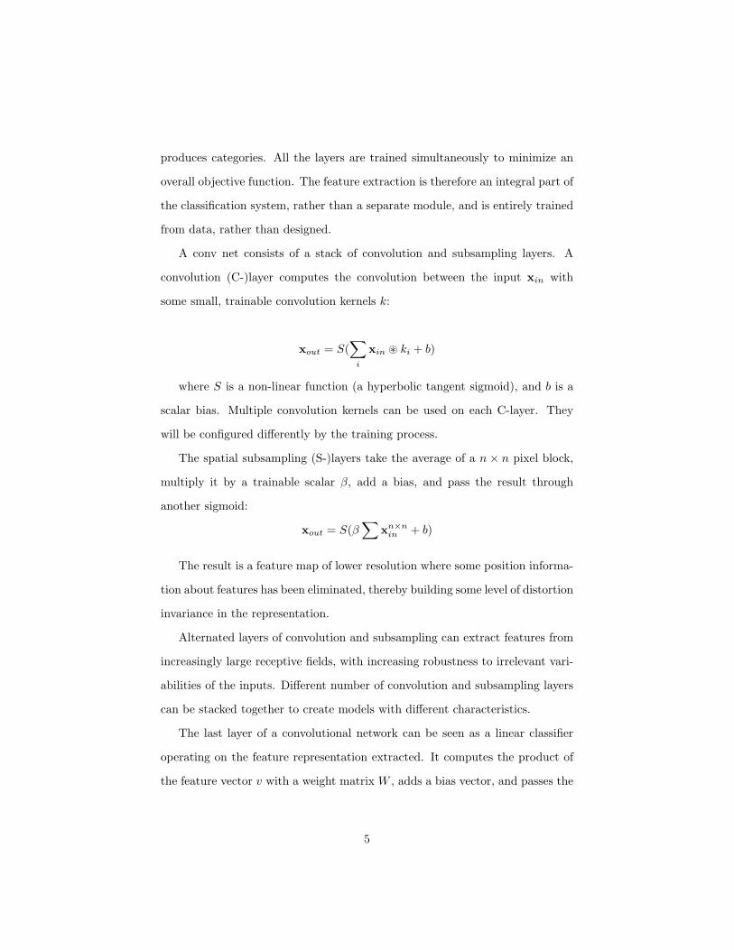
A conv net consists of a stack of convolution and subsampling layers. A
convolution (C-)layer computes the convolution between the input xin with
some small, trainable convolution kernels k:
xout = S(∑
i
xin ⊛ ki + b)
where S is a non-linear function (a hyperbolic tangent sigmoid), and b is a
scalar bias. Multiple convolution kernels can be used on each C-layer. They
will be configured differently by the training process.
The spatial subsampling (S-)layers take the average of a n × n pixel block,
multiply it by a trainable scalar β, add a bias, and pass the result through
another sigmoid:
xout = S(β∑
xn×nin + b)
The result is a feature map of lower resolution where some position informa-
tion about features has been eliminated, thereby building some level of distortion
invariance in the representation.
Alternated layers of convolution and subsampling can extract features from
increasingly large receptive fields, with increasing robustness to irrelevant vari-
abilities of the inputs. Different number of convolution and subsampling layers
can be stacked together to create models with different characteristics.
The last layer of a convolutional network can be seen as a linear classifier
operating on the feature representation extracted. It computes the product of
the feature vector v with a weight matrix W , adds a bias vector, and passes the
5
1x96x96
8x92x92
8x23x23
24x18x1824x6x6 100
5x5 convolution(8 kernels)
6x6 convolution(96 kernels)
6x6 convolution
(2400 kernels)
4x4 subsample
3x3 subsample
Figure 2.1: The architecture of the convolutional net used in this experiment.The input is an image of size 96 × 96, the system extracts 8 feature maps ofsize 92× 92, 8 maps of 23× 23, 24 maps of 18× 18, 24 maps of 6× 6, and 100dimensional feature vector. The feature vector is then transformed into a scalarin the last layer to compute the distance with target value.
result through sigmoid functions. The Euclidean distance between the output
vector and a target output vector T i is used as the loss function to be minimized:
L = ‖S(W.v + b)− T i‖2
where W is a trainable weight matrix of the last layer. T i can be a traditional
place code (one unit corresponding to the i-th element set to active, other units
inactive), i being the class label of the input x.
The network is trained by minimizing L. Gradient descent based algorithms
can be used for the optimization since all the layers are differentiable. The
training process is described in more details in later sections.
2.2 Example model
In our work, a six-layer conv net is used, as seen in figure 2.1. The layers in the
model are sequentially indexed, and named C1, S2, C3, S4, C5, and output.
In the figure, a testing image of size 96×96 is used. C1 uses 8 convolution
kernels of size 5×5 to generate 8 feature maps. There are 208 (200 on ki and
6
8 on b) trainable parameters in this layer. The output of C1 is a 8×92×92
3-dimensional array.
S2 is a 4×4 subsampling layer with 16 parameters, with output dimensions
8×23×23.
C3 uses 96 convolution kernels of size 6×6 to output 24 feature maps. The C3
layer contains 3,480 trainable parameters, with output dimensions 24×18×18.
S4 is a 3×3 subsampling layer which outputs feature maps of size 24×6×6.
C5 has 2400 kernels of size 6×6. A C5 layer outputting 100 feature maps
has 86,500 trainable parameters, about 95% of the whole system’s parameter
set. The output of the C5 layer is a 100-dimensional vector.
The output layer takes inputs from all C5 maps, transform them into a
scalar. The binary decision of whether the 96×96 has the object is based on
this scalar’s value.
2.3 Training with backpropagation
To minimize the loss function a stochastic version of the Levenberg-Marquardt
algorithm with diagonal approximation of the Hessian was used.
The whole data set can be used for multiple passes to get progressively better
results. The test error rate flattens out after about 10 passes. No significant
over-training was observed, and no early stopping was performed.
One parameter controlling the training procedure must be heuristically cho-
sen: the global step size of the stochastic gradient procedure. Best results are
obtained by adopting a schedule in which this step size is progressively decreased
from 2× 10⁻⁵ to 1× 10⁻⁶.
The convolutional nets are computationally very efficient. The training time
scales sub-linearly with dataset size in practice.
7
Chapter 3
Training the object
recognizer
In this chapter, we describe the application of the conv-nets to the image based
object recognition. This include the classification task, where objects are to be
decided whether present in the image, and the detection task where the objects
are localized within an image.
We describe how the training images are collected, labelled, and prepro-
cessed. The architectural details of conv-nets are described. We evaluate the
performance of the classification task with the recall-precision curve. We also
show some examples of the detection results.
The system described in this chapter has been implemented and tested in
a production environment. Daily processing of millions of images has been
achieved with a fast implementation of the system, and the recognizer has shown
impressive results in the real-world commercial environment.
8
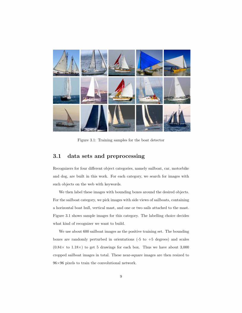
Figure 3.1: Training samples for the boat detector
3.1 data sets and preprocessing
Recognizers for four different object categories, namely sailboat, car, motorbike
and dog, are built in this work. For each category, we search for images with
such objects on the web with keywords.
We then label these images with bounding boxes around the desired objects.
For the sailboat category, we pick images with side views of sailboats, containing
a horizontal boat hull, vertical mast, and one or two sails attached to the mast.
Figure 3.1 shows sample images for this category. The labelling choice decides
what kind of recognizer we want to build.
We use about 600 sailboat images as the positive training set. The bounding
boxes are randomly perturbed in orientations (-5 to +5 degrees) and scales
(0.84× to 1.18×) to get 5 drawings for each box. Thus we have about 3,000
cropped sailboat images in total. These near-square images are then resized to
96×96 pixels to train the convolutional network.
9
Figure 3.2: The negative samples for the boat detector
The negative set are randomly cropped from a large number of images col-
lected from imageshack.com, after removing sailboat images. About 3,000 neg-
ative images are used in our experiment. By randomly cropping 5 patches from
each image, we have 15,000 negative samples for training. Figure 3.2 shows
sample image for this set.
The image samples are preprocessed carefully to remove influence of vari-
ations of color, lighting condition, and contrast. The color images are first
converted to gray scale. Then pixel intensity equalization is applied. Finally, a
19×19 high-pass filter is applied to the images. The operation makes the average
pixel intensity to be near 0, hence removes lighting condition variations.
Special attention is needed to deal with the filtering at image edges, where
for a pixel anchored with the center of the filter, not all surrounding pixels are
available. The filter coefficients that correspond to the missing pixels need to
be subtracted from the center coefficient of the filter.
10
3.2 training the recognizer
The convolutional network we used as the object recognizer has 5 layers: a
convolution layer with 8 filters of sizes 5×5, followed by a 4×4 subsampling layer,
then a second convolution layer 96 filters of sizes 6×6, and a 3×3 subsampling
layer, and another convolution layer with 2400 filters of sizes 6×6.
With this convolution network, each image patch of size 96×96 is trans-
formed into a 92×92×8 sized stack of features, then subsampled to 23×23×8.
The 8 layers of features are then combined with certain configuration by the
second batch of convolution filters to generate a 18×18×24 features, subsam-
pled to 6×6×24, and finally combined by the last convolution layer into a 100
dimensional feature vector. This feature vector is linearly combined to gener-
ate a output value. During training process, we adjust the network parameter,
through backpropagation such that for negative samples, the output value is as
close to −1.5 as possible, and for positive samples, the output value should be
pushed to near +1.5.
The stochastic gradient descent described in the previous chapter is used to
learn the parameters of the whole system. We gradually decrease the learning
step size from 2× 10⁻⁵ to 10−6 in the total 35 epochs used for training.
3.3 image classification, detection and evalua-
tions
For images larger than 96×96 in size, we can use the trained template, and
scan it through the image horizontally and vertically. Wherever a local patch
correlates with the template highly, we have a positive detection of this object.
The convolutional net we use does this scanning automatically, except that
it translates 12 pixels between two neighboring outputs, due to the two subsam-
11
pling (3×3 and 4×4) operations.
The process only detects objects of size 96×96. In reality, we wish to detect
objects of different sizes. We can either use a set of templates with different
sizes, or resize the image to different scales and use a fixed-size template which
works equivalently.
In our experiment, we systematically resize the original image into a set of 13
scales that are√2 apart, from 1/32× to 2× scaling of the image. Such scaled
images form a pyramid. Running the template with fixed 96×96 can detect
objects of all sizes ranging from 48×48 to 3072×3072.
Out of the 13 scales, only those with object size of interest are searched.
We use both an absolute size limit and a relative size bound. The choice of the
limits are empirical: the object has to be larger than 48 pixels, and it must be
larger than both 1/20 of the longer side of the image and 1/3 of the shorter side
of the image, and the object must also be smaller than the shorter side of the
image.
The performance of the system can be evaluated with two different tasks,
classification and detection. The classification task is to decide whether the
specific object is present in the image or not. This binary classification can be
measured by the recall-precision curve.
The curve can be obtained as following. For each test sample, a numerical
value is assigned by the classifier. This value is compared with pre-determined
threshold θ. If the value is higher than the threshold, then the system thinks at
least one instance of the object is present.
A testing sample with a value above the threshold falls in 2 categories. It is
a true positive (TP ) if it comes from the positive training set. And it is a false
positive (FP ) if it comes from the negative training set, i.e., it does not actually
contain the object.
12
On the other hand, a testing sample with a value lower than the threshold
can be either a true negative (TN) if it is from the negative set, or a false
negative (FN) if it is from the positive set and in fact does contain the object.
The above 4 elements of the confusion matrix contains all the information
about the classifier’s performance. But in the image retrieval applications, the
following two values are usually extracted from the confusion matrix to measure
specific aspects of the system.
The recall, TP/(TP + FN), is the number of true positive samples normal-
ized by the number of samples in the positive training set. This describes the
probability of detecting a positive testing sample. The recall value ranges from
0 to 1.
The precision, TP/(TP +FP ), is defined as among the samples with values
above the threshold, what percentage is true positives.
For a given testing set, each threshold values gives us a recall-precision pair.
And the recall-precision curve can be obtained by increasing the threshold from
minimum value to maximum.
Ideally, we would like to have a system with both high recall and hight
precision. But these two measures usually work against each other. We can
lower the threshold to get a higher recall rate, but then the precision will also
go lower. A suitable threshold can be chosen according to the requirement of
the application, depending whether a specific recall rate or a precision rate is
more desirable.
Figure 3.3 shows the recall-precision curve for the sailboat classification.
The testing set consists of 50 positive samples and 200 negative samples. The
threshold is adjusted in the range [0, 100] to obtain the data points on the curve.
The detection task is similar to the classification except some post-processings
are needed. For each scale, we threshold the array of the outputs. Those
13
0
0.1
0.2
0.3
0.4
0.5
0.6
0.7
0.8
0.9
1
0 0.1 0.2 0.3 0.4 0.5 0.6 0.7 0.8 0.9 1
Pre
cisi
on (
%)
Recall (%)
Recall-precision for boat
Figure 3.3: The recall-precision curve of the boat classifier
points with values above threshold are then transformed into equivalent bound-
ing boxes in the original image scale.
The bounding boxes collected from all scales are then compared with each
other to remove redundant ones. For a pair of neighboring boxes with significant
overlapping, the one with a smaller recognizer output value is removed. This is
based on the observation that an image patch with an object usually produce a
cluster of neighboring bounding boxes.
The detection performance is evaluated in a less rigorous way. We simply
run the system on the 50 positive images. The system’s localization results
are compared with the manual labelling. With a threshold of 60, there are
4 images where the boats are missed by the detector, and there is one false
positive detection on a non-boat background area. The correct detection rate is
therefore above 90%. Figure 3.4 shows some sample images with the detection
14
Figure 3.4: The sailboat samples with superposed detection bounding boxes
result bounding boxes drawn.
3.4 retraining with false positive samples
One difficulty in building an object recognizer is the lack of good negative train-
ing samples. Conceptually the positive samples populate only a small neigh-
borhood in the hyperspace due to their visual similarities, while the negative
samples span the remaining vast space. We often need a very large negative set
of samples to cover such space.
In the previous experiments, we collected the negative set by randomly crop-
ping image patches from non-object images. Even though this set is much bigger
than the positive set, these samples do not cover the non-object space well. This
results in a lot of false positives yielded by the classifier.
15
Figure 3.5: The targeted negative samples
In order to learn the decision boundary separating the positive and negative
spaces, we only need the samples that are close to the boundary on both sides.
That is, we need negative samples are easily confused with the positives. These
samples lie near the decision boundary.
The detector built in the previous experiment can help us to pick such neg-
ative samples efficiently. We run the learned detector through the negative set
and pick up the false positive patches, as shown in figure 3.5. These false pos-
itives are then merged into the negative training set to train a more refined
system. In the literature, this process is called bootstrapping [43].
In the sailboat experiment, we collected 3,500 image patches from the neg-
ative set. These patches are then perturbed to generate 7,000 samples. The
system is re-trained in the same way using this new training data. In our ex-
periment, we observed that the training process converges with less number of
epochs to a small training error. Figure 3.6 draws both the curve obtained in
16
0
0.1
0.2
0.3
0.4
0.5
0.6
0.7
0.8
0.9
1
0 0.1 0.2 0.3 0.4 0.5 0.6 0.7 0.8 0.9 1
Pre
cisi
on (
%)
Recall (%)
Recall-precision for boat
targeted negativesrandom negatives
Figure 3.6: Comparison of the recall-precision curves of the original classifier,and of the classifier trained with targeted negative samples
the previous sections and the curve with the new system trained with the com-
bined negative set. For the same recall rate, the precision rate is increased by
10% to 15%. The retraining with the newly collected data works very well.
3.5 why high precision for classification is hard
The recall-precision curve of the sailboat classifier in previous section is obtained
on a test set with 50 positive samples and 200 negative samples. The ratio
λ between the number of negative samples Nn versus the number of positive
samples Np, λ = Nn/Np, can change when we chose a different test set. This
ratio λ influence directly the result of the precision.
This can be seen by transforming the definition of the precision:
17
0
0.1
0.2
0.3
0.4
0.5
0.6
0.7
0.8
0.9
1
0 0.1 0.2 0.3 0.4 0.5 0.6 0.7 0.8 0.9 1
Pre
cisi
on (
%)
Recall (%)
Recall-precision for boat
ratio = 4ratio = 32
Figure 3.7: Comparison of the recall-precision curves of test set with differentnegative to positive ratios
where the true positive rate (TPr) and the false positive rate (FPr) are both
only dependent on the threshold θ. Therefore, when we increase the ratio λ,
TPr and FPr remain the same, while the precision decreases.
The reason for precision to be dependent on λ is that precision combines
results from both the positive set and negative set, and is therefore prior de-
pendent. Recall, on the other hand, is only related to the positive set.
Figure 3.7 shows the two recall-precision curves with different ratio λ for
the same sailboat classifier. The original curve is obtained with 200 negative
samples, and ratio 4. The red curve is for a negative set of 1600 samples, and
18
0
0.1
0.2
0.3
0.4
0.5
0.6
0.7
0.8
0.9
1
0 0.1 0.2 0.3 0.4 0.5 0.6 0.7 0.8 0.9 1
Pre
cisi
on (
%)
Recall (%)
Recall-precision for motorbike
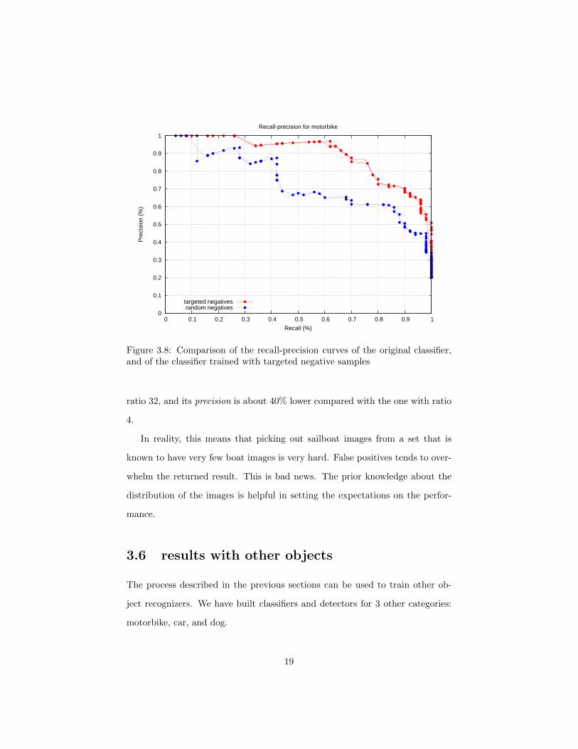
targeted negativesrandom negatives
Figure 3.8: Comparison of the recall-precision curves of the original classifier,and of the classifier trained with targeted negative samples
ratio 32, and its precision is about 40% lower compared with the one with ratio
4.
In reality, this means that picking out sailboat images from a set that is
known to have very few boat images is very hard. False positives tends to over-
whelm the returned result. This is bad news. The prior knowledge about the
distribution of the images is helpful in setting the expectations on the perfor-
mance.
3.6 results with other objects
The process described in the previous sections can be used to train other ob-
ject recognizers. We have built classifiers and detectors for 3 other categories:
motorbike, car, and dog.
19
0
0.1
0.2
0.3
0.4
0.5
0.6
0.7
0.8
0.9
1
0 0.1 0.2 0.3 0.4 0.5 0.6 0.7 0.8 0.9 1
Pre
cisi
on (
%)
Recall (%)
Recall-precision for car
targeted negativesrandom negatives
Figure 3.9: Comparison of the recall-precision curves of the original classifier,and of the classifier trained with targeted negative samples
The motorbike category is very similar to the boat in that most images have
side views of the objects. The car images have more view variations. The dog
category is even more challenging since the objects are not rigid and can have
different shapes depending on the configuration of the body parts.
The car training images contain mostly the between-front-and-side view,
where at least one head light and its closest wheel are visible. For the dog rec-
ognizer, we choose to recognize only the head part, and with frontal or between-
front-and-side views.
The same procedure of labeling, training and evaluation is used for these
objects. Between 500 to 900 images are labeled for each category, and the conv-
nets of the same architecture are trained. The trained detectors are then used
to collect false positive samples from the negative training set. The results are
combined with the randomly chosen negative samples to retrain the recognizer.
20
0
0.1
0.2
0.3
0.4
0.5
0.6
0.7
0.8
0.9
1
0 0.1 0.2 0.3 0.4 0.5 0.6 0.7 0.8 0.9 1
Pre
cisi
on (
%)
Recall (%)
Recall-precision for dog
targeted negativesrandom negatives
Figure 3.10: Comparison of the recall-precision curves of the original classifier,and of the classifier trained with targeted negative samples
Figure 3.8 shows the recall-precision curve for the motorbike recognizer. The
valuation set contains 50 positive samples and 200 negative samples. The lower
curve is from the system trained with random negative samples, while the other
curve is from the system trained with targeted negative samples. The retraining
boosts the precision rate by 10% to 20%. Figure 3.9 and figure 3.10 shows the
performances of the car and dog recognizers, respectively. Both these recog-
nizers have a much higher precision rate when retrained with targeted negative
samples.
21
Chapter 4
Fast Implementation of
Convolutions
The convolutional network has shown a remarkable capability for the object
recognition task, as we have shown in the last chapter. In order to apply this
technology in the real world environment, an efficient implementation of the
system is needed. In this chapter, we describe the work to implement the con-
volutional network on the GPU. The modern GPUs have thousands of cores
capable of general computing. These cores can be programmed to do massive
parallel computing on the desktop environment. We will show that the most
computationally intensive part of the recognition system, the convolution op-
eration, can be easily parallelized to achieve computing performance far above
running a traditional CPU.
22
4.1 Convolution operation is computationally in-
tensive
We first profile the convolutional net based object detection system to find the
hot spot, the component that takes up most of the computing time. The hot
spot is then optimized to speed up the system.
The system consists of three parts, the image preprocessing, convolution
nets, and the post-processing. The image preprocessing includes the color to
grayscale conversion, resizing, histogram equalization, filtering. These opera-
tions are well understood in terms of their computational complexities.
In the second step, the preprocessed image is fed through the convolution
net to produce a two-dimensional confidence map, representing the confidences
of a local image patch being of the target object. The post-processing marks
the locations where objects are detected, based on the confidence map.
In this work, we first implement a reference system in C++. The the runtime
complexity of the various steps can be measured with profilers. Figure 4.1 shows
a call graph when running the system with a 216×120 test image on an Intel
Q8200 CPU. Each node stands for one function, annotated with the accumulated
running time.
We can see that the overall detection on the image takes 29.1 ms, while
the convolutional operation, op convolution, takes 20.5 ms, which accounts for
about 70% of the whole process. It is obvious that optimizing the convolutional
operation would speed up the entire process.
In the next section, we analyze the complexity of the convolution operation,
and show that it can be easily parallelized.
23
object_detect(lenet7&, _IplIma... 29.1ms
lenet7::fprop(boost::multi_arr... 28.4ms
op_convolution(boost::multi_ar... 20.5ms
Figure 4.1: The call graph annotated with runtime complexity
4.2 Computational complexity of convolutions
Convolution operations can be applied to two arrays of the same dimensions.
The convolutions between two 1-dimensional vectors are often used in audio sig-
nal processing. The convolutions between two 2-dimensional arrays are popular
in image processing. The convolution net in this work uses a generalized version
of the 3-dimensional convolution.
The 1-dimensional convolutions between two vectors A and B, of size N and
k respectively, where N≫k, can be described as follows. From the longer vector
A of size N, we successively take sub-vectors of size k, with one element shifting
each time, and take the inner product between it and the smaller vector B,
the result is one element in the output vector C, as shown in 4.1. Obviously
this process involves two nested loops, with the inner loop computing the inner
product, and the computational complexity is O(k(N − k + 1)).
Listing 4.1: convolution between 1-d vectors
1 for ( int i =0; i<(N−k+1); ++i ) {2 C[ i ] = 0 ;3 for ( int j =0; j<k ; ++i )4 C[ i ] += A[ i+j ] ∗ B[ j ] ;5 }
Similarly, the complexity for the 2-d convolution between two arrays of size
N×N and k×k is O(k2(N − k+1)2) with 4 nested loops. And 3-d convolutions
24
between arrays of size N×N×N and k×k×k has complexity of O(k3(N−k+1)3)
with 6 nested loops.
The convolution net uses a generalized version of the 3-d convolution de-
scribed above. The first input array of the operation is of size D×N×N, and
the second input, the kernel array, is of size (d×P)×k×k. The first input is
considered as a stack of 2-d features maps, where the stack dimension is treated
differently from the other two dimensions of the feature maps.
For the operation, we take d feature maps out of the D maps, of size d×N×N,
and apply the regular 3-d convolution with the d×k×k subset of the kernel array.
We get an output array of size 1×(N-k+1)×(N-k+1), which can be degenerated
into a 2-d (N-k+1)×(N-k+1) matrix. We repeat this process P times, and stack
the output matrices together to get a 3-d array of size P×(N-k+1)×(N-k+1).
The choices of d out of D feature maps from the first input can be configured
in a table of size d×P whose elements range between 0 and D-1.
The operation described above can be implemented with 6-level nested loop
with P, N-k+1, N-k+1, d, k, k iterations respectively. The first 3 loops iterate
through each element of the P×(N-k+1)×(N-k+1) sized output array, and each
element is the inner product of two d×k×k arrays. The following code snippet
in 4.2 shows a detailed implement of the convolution operation.
25
Listing 4.2: Convolution operation
1 void op conv ( const f loat ∗o1 ,2 int extent 1 0 , int extent 1 1 , int extent 1 2 ,3 int s t r i d e 1 0 , int s t r i d e 1 1 , int s t r i d e 1 2 ,4 const f loat ∗o2 ,5 int extent 2 0 , int extent 2 1 , int extent 2 2 ,6 int s t r i d e 2 0 , int s t r i d e 2 1 , int s t r i d e 2 2 ,7 f loat ∗o3 ,8 int extent 3 0 , int extent 3 1 , int extent 3 2 ,9 int s t r i d e 3 0 , int s t r i d e 3 1 , int s t r i d e 3 2 ,
10 const int ∗o4 ,11 int extent 4 0 , int extent 4 1 ,12 int s t r i d e 4 0 , int s t r i d e 4 1 ,13 const f loat ∗o5 ,14 int s t r i d e 5 0 )15 {16 for ( int h=0; h < ex t en t 3 0 ; ++h) {17 for ( int i =0; i < ex t en t 3 1 ; ++i ) {18 for ( int j =0; j < ex t en t 3 2 ; ++j ) {19 const f loat ∗p3 1 = o1 + i ∗ s t r i d e 1 1 + j ∗ s t r i d e 1 2 ;20 const f loat ∗p3 2 = o2 + (h∗ ex t en t 4 0 ) ∗ s t r i d e 2 0 ;2122 f loat f = 0 ;23 for ( int k=0; k < ex t en t 4 0 ; k++) {24 const f loat ∗p2 1 = p3 1 + o4 [ k∗ s t r i d e 4 0+h ]∗ s t r i d e 1 0 ;25 const f loat ∗p2 2 = p3 2 + k ∗ s t r i d e 2 0 ;2627 for ( int m=0; m < ex t en t 2 1 ; ++m) {28 const f loat ∗p1 1 = p2 1 + m∗ s t r i d e 1 1 ;29 const f loat ∗p1 2 = p2 2 + m∗ s t r i d e 2 1 ;3031 for ( int n=0; n < ex t en t 2 2 ; ++n) {32 f += ∗p1 1++ ∗ ∗p1 2++;33 }34 }35 }36 f loat ∗p0 3 = o3+h∗ s t r i d e 3 0+i ∗ s t r i d e 3 1+j ∗ s t r i d e 3 2 ;37 const f loat ∗p0 5 = o5 + h∗ s t r i d e 5 0 ;38 ∗p0 3 = stds igmoid ( f + ∗p0 5 ) ;39 }40 }41 }42 }
The convolution operation described in 4.2 has a running cost of O(dP (N −
k + 1)2k2). In order to get a concrete idea of the run time complexity of the
convolutional net, let us consider using a real image with size 120×216. The feed
forward convolution net has 3 convolution layers and 2 subsampling layers. The
first convolution layer has d = 1, P = 8, k = 5, and it generates an output array
of size 8×116×212. The computational cost is 1×8×116×212×5×5 = 4.9×10⁶
Table 4.1: The count of floating operations in convolution layers with an exampleimage
fused multiply-add (FMA) operations, or about 10 millions floating operations,
with each FMA counted as 2 floating operations. The following subsampling
layer has k = 4, generating output of size 8 × 29 × 53. The next convolution
layer has d = 4, P = 24, k = 6, costing 3.9×10⁶ FMAs, and generates an output
of size 24×24×48. The following subsampling layer has k = 3, which brings the
output to 24 × 8 × 16. The last convolution layer has d = 24, P = 100, k = 6,
which takes 2.8 × 10⁶ FMAs to run and generates a confidence map of size
100× 3× 11.
With this example image, the total computational cost for convolutions adds
up to about 23 million floating operations, as shown in the first column of the
table 4.1. Profiled on an Intel Core2Quad 2.3 GHZ CPU Q8200, running in a
single thread, the convolutions add up to about 20 ms, as shown in the second
column in the same table. This yields about 1.2 GFLOPS performance. Note
that this performance is not only related to the hardware, but also the code
implementation and the compiling tools.
4.3 Parallelize the Convolution Operations
The previous sections have analyzed the computational complexity of the conv
nets, and established that the most runtime intensive part is the convolution
operations. To speed up the system, it is essential to implement the convolution
operation efficiently.
27
The convolution operations turn out to be very amenable to parallelization.
The key is to identify the parts that are independent of each other and can be run
by a separate thread. As previously analyzed, the operation consists of 6 nested
loops. The 3 inner-most loops compute the inner product between two d×k×k
arrays. These inner product computations are inherently independent from each
other. To make this fact more obvious, we can factor out the inner most 3 loops
and put them in a standalone function, as shown in 4.3, where there are 3 extra
arguments compared with the function op conv described in 4.2, namely, h, i,
j. This tuple identifies which inner product the function is computing.
Listing 4.3: Function with the 3 inner loop in the convolution operation
1 void op conv kerne l ( . . . , int h , int i , int j )2 {3 const f loat ∗p3 1 = o1 + i ∗ s t r i d e 1 1 + j ∗ s t r i d e 1 2 ;4 const f loat ∗p3 2 = o2 + (h∗ ex t en t 4 0 ) ∗ s t r i d e 2 0 ;56 f loat f = 0 ;7 for ( int k=0; k < ex t en t 4 0 ; k++) {8 const f loat ∗p2 1 = p3 1 + s t r i d e 1 0 ∗ o4 [ k∗ s t r i d e 4 0+h ] ;9 const f loat ∗p2 2 = p3 2 + s t r i d e 2 0 ∗ k ;
1011 for ( int m=0; m < ex t en t 2 1 ; ++m) {12 const f loat ∗p1 1 = p2 1 + m∗ s t r i d e 1 1 ;13 const f loat ∗p1 2 = p2 2 + m∗ s t r i d e 2 1 ;1415 for ( int n=0; n < ex t en t 2 2 ; ++n) {16 f += ∗p1 1++ ∗ ∗p1 2++;17 }18 }19 }20 f loat ∗p0 3 = o3 + h∗ s t r i d e 3 0+i ∗ s t r i d e 3 1+j ∗ s t r i d e 3 2 ;21 const f loat ∗p0 5 = o5 + h∗ s t r i d e 5 0 ;22 ∗p0 3 = stds igmoid ( f + ∗p0 5 ) ;23 }
The outer 3 loops iterate through each element of the output array. Each
iteration step invokes the above op conv kernel to compute the inner product,
as shown in 4.4.
28
Listing 4.4: Convolution operation
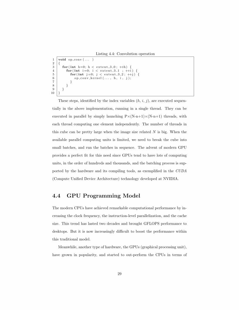
1 void op conv ( . . . )2 {3 for ( int h=0; h < ex t en t 3 0 ; ++h) {4 for ( int i =0; i < ex t en t 3 1 ; ++i ) {5 for ( int j =0; j < ex t en t 3 2 ; ++j ) {6 op conv kerne l ( . . . , h , i , j ) ;7 }8 }9 }
10 }
These steps, identified by the index variables (h, i, j), are executed sequen-
tially in the above implementation, running in a single thread. They can be
executed in parallel by simply launching P×(N-n+1)×(N-n+1) threads, with
each thread computing one element independently. The number of threads in
this cube can be pretty large when the image size related N is big. When the
available parallel computing units is limited, we need to break the cube into
small batches, and run the batches in sequence. The advent of modern GPU
provides a perfect fit for this need since GPUs tend to have lots of computing
units, in the order of hundreds and thousands, and the batching process is sup-
ported by the hardware and its compiling tools, as exemplified in the CUDA
(Compute Unified Device Architecture) technology developed at NVIDIA.
4.4 GPU Programming Model
The modern CPUs have achieved remarkable computational performance by in-
creasing the clock frequency, the instruction-level parallelization, and the cache
size. This trend has lasted two decades and brought GFLOPS performance to
desktops. But it is now increasingly difficult to boost the performance within
this traditional model.
Meanwhile, another type of hardware, the GPUs (graphical processing unit),
have grown in popularity, and started to out-perform the CPUs in terms of
29
computational power. The GPUs have a different design philosophy. They
usually have hundreds, even thousand of computing cores, compared with the
CPUs with just dual cores or quad cores. Even though GPU cores usually have
lower clock frequencies, and simplified control logic, their combined performance
can easily top off the CPUs.
The peak performance of the GPU by NVIDIA has reached 1 teraflops in
2009, 10 times of Intel CPU’s 100 gigaflops performance. And the gap has been
increasing since then.
The GPU-enabled program runs in two modes. Most part of the program
runs on the CPU, or the host. The part that needs to be parallelized runs on
the GPU, or the device. The host and device exchange data by copying between
the host memory and the device memory.
The CUDA framework extends the C++ syntax with a few key words that
are recognized by its compiler nvcc. Functions running on the device are prefixed
with global . Multiple copies of a device function can be launched simultane-
ously. Each one runs in its own thread, and is supplied with special variables
blockIdx and threadIdx to identify itself.
The following code snippet in 4.5 is a rewrite of the function op conv kernel
in 4.3. The compiler recognizes this function as a device function since it’s
prefixed with global . It will be compiled separately into GPU machine code.
Notice that its function arguments do not include the tuple (h, i, j). Instead,
they are computed from the special variables blockIdx and threadIdx.
This device function is remarkably similar to the regular CPU version. The
only difference is that since threads are launched in batches, some redundant
threads may be launched. We need to tell these threads to return without doing
anything, as shown on line 9 and 10. The variable c table on line 7 is a global
variable in the constant memory, a kind of memory specific to the GPU. We
30
store the configure in constant memory for faster access.
Listing 4.5: Device function computing inner product
1 g l o b a l void op conv kerne l ( . . . )2 {3 int h = blockIdx . z ∗ blockDim . z + threadIdx . z ;4 int i = blockIdx . y ∗ blockDim . y + threadIdx . y ;5 int j = blockIdx . x ∗ blockDim . x + threadIdx . x ;67 const int ∗o4 = &c t ab l e [ t b l o f f s e t ] ;89 i f ( ! (h < ex t en t 3 0 && i < ex t en t 3 1 && j < ex t en t 3 2 ) )
10 return ;1112 const f loat ∗p3 1 = o1 + i ∗ s t r i d e 1 1 + j ∗ s t r i d e 1 2 ;13 const f loat ∗p3 2 = o2 + (h∗ ex t en t 4 0 ) ∗ s t r i d e 2 0 ;1415 f loat f = 0 ;16 for ( int k=0; k < ex t en t 4 0 ; ++k) {17 const f loat ∗p2 1 = p3 1 + s t r i d e 1 0 ∗ o4 [ k ∗ s t r i d e 4 0 + h ] ;18 const f loat ∗p2 2 = p3 2 + s t r i d e 2 0 ∗ k ;1920 for ( int m=0; m < ex t en t 2 1 ; ++m ) {21 const f loat ∗p1 1 = p2 1 + m ∗ s t r i d e 1 1 ;22 const f loat ∗p1 2 = p2 2 + m ∗ s t r i d e 2 1 ;2324 for ( int n=0; n < ex t en t 2 2 ; ++n)25 f += ∗p1 1++ ∗ ∗p1 2++;26 }27 }28 f loat ∗p0 3 = o3 + h∗ s t r i d e 3 0 + i ∗ s t r i d e 3 1 + j ∗ s t r i d e 3 2 ;2930 const f loat ∗p0 5 = o5 + h ∗ s t r i d e 5 0 ;31 ∗p0 3 = stds igmoid ( f + ∗p0 5 ) ;32 }
The function op conv in 4.4 executes op conv kernel in sequence with a single
thread. This function also needs to be modified to instead launch a grid of
P×(N-k+1)×(N-k+1) threads, with each thread running a copy of the device
function.
CUDA provides a symbol 〈〈〈〉〉〉 between the device function name and its
parentheses to mark a thread-launching point. The compiler will fill in the
routine instructions that create threads, copy the device function machine code
to GPU, and start the GPU threads. The code in 4.6 shows the new op conv
that launches parallel threads, instead of having 3 nested loops.
The arguments passed into the 〈〈〈〉〉〉 specify the cube of threads, P×(N-
31
k+1)×(N-k+1) in our case. These threads are grouped into a 2-level hierarchy,
since the number of threads may exceeds the number of available execution units.
The threads in a block, whose size is specified by block size, are guaranteed to
execute at the same time. The P×(N-k+1)×(N-k+1) threads are grouped into
a grid of blocks, as specified by grid size. The grouping of threads is device
dependent, and can have an impact on the execution speed.
Listing 4.6: Host function for convolution operation
1 #define BLOCKWIDTH 162 #define BLOCK HEIGHT 163 void op conv ( . . . )4 {5 int s z 0 = ( int ) c e i l ( e x t en t 3 0 / ( f loat ) 1 ) ;6 int s z 1 = ( int ) c e i l ( e x t en t 3 1 / ( f loat ) BLOCK HEIGHT ) ;7 int s z 2 = ( int ) c e i l ( e x t en t 3 2 / ( f loat ) BLOCKWIDTH ) ;89 dim3 b l o c k s i z e ( BLOCKWIDTH, BLOCK HEIGHT, 1 ) ;
10 dim3 g r i d s i z e ( sz 2 , sz 1 , s z 0 ) ;1112 op conv kerne l<<< g r i d s i z e , b l o c k s i z e >>>( . . . ) ;13 }
4.5 Performance improvement with GPU
In this section, we will profile the GPU implementation of convolutions as de-
scribed in 4.5 and 4.6, tested on a NVIDIA GTX 560 Ti GPU. We show that
with the small code changes, the convolution operation can be run on the GPU
with 39× speedup, compared against running on an Intel CPU using a single
core.
We use the same testing image of size 216×120, and the same convolution
net with layers c-s-c-s-c, with the c-layer filter kernels of size 5×5, 6×6, 6×6,
and the s-layer subsampling rates of 4×4 and 3×3. The configuration tables for
the c-layers have parameters d×P as 1×8, 4×24, and 24×100.
The GTX 560 Ti GPU has 384 cores with clock frequency 1.7GHz. The
GPU has 1GB global memory of clock rate 2GHz. It has CUDA capability
Table 4.2: Comparing the running time of CPU and GPU implementations
version 2.1. This capability mainly concerns the hardware’s thread scheduling,
memory accessing mechanism etc.
We use the CUDA SDK toolkit version 4.0, including compiler, debugger,
profiler, and runtime library. The NVIDIA profiler computeprof generates de-
tailed information about the function running time, as well as a time trace of
the entire program.
Table 4.2 shows the real running time of the 3 op conv operations, on CPU
and GPU respectively, and the speedups. The column for CPU is the same as re-
ported in table 4.1. On average, the GPU implementation achieves 39× speedup
against the one that runs on a CPU. This is about 46 GFLOPS performance.
The profiler computeprof also generates a time trace of the program, as
shown in 4.2. This width plot shows the time stamp of various device functions,
represented by dark colored bars. The blank area is when the code is running
on the CPU. The unit of the plot is micro-second.
object_detect : 2.6 ms
fprop : 1.8 ms
op_convolution : 0.8 ms
Figure 4.2: The time trace of the object detection program
In the time trace, the 3 op convolution invocations and 2 op subsamples add
33
up to about 0.8 ms, decreased from the 22.4 ms of the CPU version. They
account for 30% of the running time of object detect, unlike in 4.1 where they
takes more than 70% of the running time.
The preprocessing part of the fprop, where the image is resized, filtered and
histogram equalized, uses the NPP library routines for GPU. Using function
from NPP also gains some speedup against the OpenCV library routines for
CPU.
The speedup of the system’s overall running time is governed by the Amdahl’s
law. The law formulates the speedup as a function on the runtime percentage
p of the part of code that can be parallelized, and the level of parallelization
N : 1/[(1 − p) + p/N ]. It tells the bad news about the parallelization. Assume
p is 50%, then when N approximates infinity, the speedup saturates at 2. That
is, we can at most get 2× speedup, no matter how much effort we put into
parallelizing the 50% of the program that can be parallelized.
In our work, about 90% of the entire object detect procedure can be paral-
lelized and run on a GPU. Hence it can reach about 10× speedup in theory.
The example testing image of size 216×120 takes about 2.6 ms to run a system
with the afore mentioned GPU, down from 20 ms on an Intel CPU.
4.6 Modular Design of Convolution Net
To close the discussion about the implementation, we briefly describe the data
structures and functions used. The functions described in the previous sections,
such as the op conv in 4.2, are low level functions which use arguments of plain
pointers and integers. These functions need to be wrapped in higher level ones
that are more descriptive and easier to understand anddebug.
The basic data structure used is the multi array type from the boost library.
It is a C++ template class parameterized with the element type and the dimen-
34
sionality of the array. The inputs and outputs of the convolution operation are
3-dim arrays with floating point elements, as multi array〈float, 3〉.
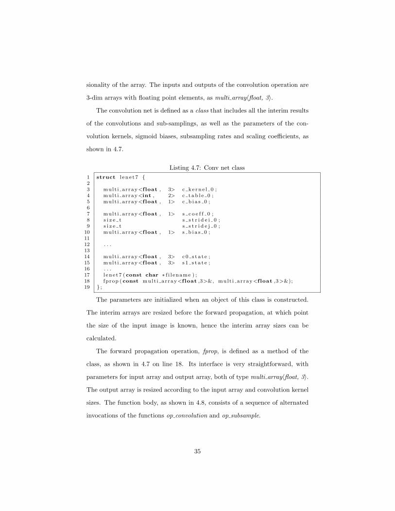
The convolution net is defined as a class that includes all the interim results
of the convolutions and sub-samplings, as well as the parameters of the con-
volution kernels, sigmoid biases, subsampling rates and scaling coefficients, as
shown in 4.7.
Listing 4.7: Conv net class
1 struct l e n e t 7 {23 mult i a r ray<f loat , 3> c k e r n e l 0 ;4 mult i a r ray<int , 2> c t a b l e 0 ;5 mult i a r ray<f loat , 1> c b i a s 0 ;67 mult i a r ray<f loat , 1> s c o e f f 0 ;8 s i z e t s s t r i d e i 0 ;9 s i z e t s s t r i d e j 0 ;
10 mult i a r ray<f loat , 1> s b i a s 0 ;1112 . . .1314 mult i a r ray<f loat , 3> c 0 s t a t e ;15 mult i a r ray<f loat , 3> s 1 s t a t e ;16 . . .17 l en e t 7 ( const char ∗ f i l ename ) ;18 fprop ( const mult i a r ray<f loat ,3>&, mult i a r ray<f loat ,3>&);19 } ;
The parameters are initialized when an object of this class is constructed.
The interim arrays are resized before the forward propagation, at which point
the size of the input image is known, hence the interim array sizes can be
calculated.
The forward propagation operation, fprop, is defined as a method of the
class, as shown in 4.7 on line 18. Its interface is very straightforward, with
parameters for input array and output array, both of type multi array〈float, 3〉.
The output array is resized according to the input array and convolution kernel
sizes. The function body, as shown in 4.8, consists of a sequence of alternated
invocations of the functions op convolution and op subsample.
35
Listing 4.8: The forward propagation method
1 void l e n e t 7 : : fprop ( const mult i a r ray<f loat , 3>& in ,2 mult i a r ray<f loat , 3>& out )3 {4 // r e s i z e the inter im and output arrays5 . . .6 op convo lut ion ( in , c k e rn e l 0 , c t ab l e 0 ,7 c b i a s 0 , c 0 s t a t e ) ;89 op subsample ( c0 s t a t e , s s t r i d e i 0 , s s t r i d e j 0 ,
10 s c o e f f 0 , s b i a s 0 , s 1 s t a t e ) ;11 . . .12 }
The convolution operation is implemented in the function op convolution.
The inputs to this function are the 3-dimensional input array in, the stack
of convolution kernels kernel. The output out and the inputs are all of type
multi array〈float, 3〉. The function is also passed in the configure table table
and the sigmoid bias as bias. This function invokes the op conv in 4.2, by
extracting the data pointer, dimension sizes, and strides.
Listing 4.9: The high level function for the convolution operation
1 void op convo lut ion ( const mult i a r ray<f loat , 3>& in ,2 const mult i a r ray<f loat , 3>& kerne l ,3 const mult i a r ray<int , 2>& table ,4 const mult i a r ray<f loat , 1>& bias ,5 mult i a r ray<f loat , 3>& out )
There have been other independent research efforts on implementing fast
convolutional networks with GPUs. The one in [44] implements 2D convolution
with highly-optimized GPU code for training a large convolutional network.
36
Chapter 5
Object Recognition System
We have described an object recognizer based on convolution networks, and its
GPU implementation in the previous chapters. To make the technology usable in
the real production environment, a robust and scalable infrastructure is needed
to support the recognition engine. More importantly, the system should be able
to interact with the outside world.
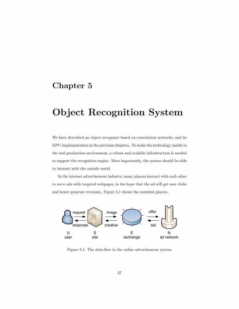
In the internet advertisement industry, many players interact with each other
to serve ads with targeted webpages, in the hope that the ad will get user clicks
and hence generate revenues. Figure 5.1 shows the essential players.
Uuser
Ssite
Eexchange
Nad network
offer
bid
request
response
image
creative
Figure 5.1: The data-flow in the online advertisement system
37
In the process, the internet user browses a certain webpage by sending a
request to the website. The requested webpage includes fixed contents (texts,
images, and videos), as well as spaces reserved for ads that needs to be decided
dynamically.
In our case, the ads are decided based on the prominent image on the current
page. The website sends the image URL to the exchange server. The exchange
server then offers to “sell” the ad space to the highest bidder. Our system acts
as the ad network in this scenario. In this role, we have an inventory of ads to be
served to webpages. Equipped with our object recognition system, we can find
the optimal webpages by understanding the image. And we bid for the optimal
ad spaces, under the assumption that serving ads on the right pages will garner
higher clicking rates.
Therefore, we need to interact with the exchange server. Our system should
able to receive recognition request over the web, retrieve the requested image,
give the image an unique ID, send the image into the recognition engines to be
processed, and send back the recognition result once it is done.
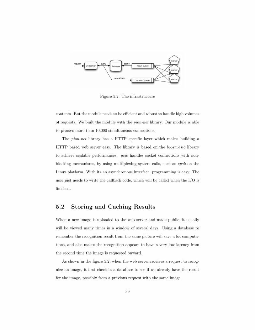
As shown in 5.2, our system includes a high throughput webserver responding
to web requests, a database that stores the recognition results, a queuing system
that hold temporarily requests and results, and a recognition engine that takes
requests from the queue and produce recognition metadata on the requested
images.
In the following sections, we discuss each subsystem.
5.1 Webserver
At the front end, the system receives web requests from the ad exchange. We
need a web server module for the task. Its functionality is simpler than a
traditional web server, such as Apache, in that it does not need to serve static
38
webserver database
request queue
result queue
worker
worker
worker
request query cache
submit jobs
Figure 5.2: The infrastructure
contents. But the module needs to be efficient and robust to handle high volumes
of requests. We built the module with the pion-net library. Our module is able
to process more than 10,000 simultaneous connections.
The pion-net library has a HTTP specific layer which makes building a
HTTP based web server easy. The library is based on the boost::asio library
to achieve scalable performances. asio handles socket connections with non-
blocking mechanisms, by using multiplexing system calls, such as epoll on the
Linux platform. With its an asynchronous interface, programming is easy. The
user just needs to write the callback code, which will be called when the I/O is
finished.
5.2 Storing and Caching Results
When a new image is uploaded to the web server and made public, it usually
will be viewed many times in a window of several days. Using a database to
remember the recognition result from the same picture will save a lot computa-
tions, and also makes the recognition appears to have a very low latency from
the second time the image is requested onward.
As shown in the figure 5.2, when the web server receives a request to recog-
nize an image, it first check in a database to see if we already have the result
for the image, possibly from a previous request with the same image.
39
If the image is seen for the first time, the front end puts the request and
image ID in a request queue to be processed by the back end. When the back
end finishes the processing, the result will be put in the result queue and then
stored into the database. If this image is requested again later, we can get an
immediate answer.
We can see that the web server only reads from the database, it never
write directly into the database. Traditional SQL databases, including MySQL,
tend to have slow reads. To bridge the fast web server module and the slower
database, we need some caching mechanism.
We use the memcached to cache MySQL reads. It uses the image ID as
the hashing key to retrieve the value that has the metadata about the image.
This pairing usage of memcached and MySQL is a quite common practice in the
industry.
5.3 Queuing System
The queuing system is the central link that connects the front end of web server
and the back end of a set of worker instances, as shown in figure 5.2. When
the web server finds that the request it received does not have an answer in
the database, it puts the request in the request queue. The workers later pick
up the requests and process them, and put the recognition results in the result
queue when done. The contents in the result queue are periodically taken out
and inserted into the database in the front end, so that they can be retrieved
and sent back to the requesting clients.
With the queuing system, the front end and the back end loosely coupled.
They are mutually unaware of the existence of each other. This makes the
system more robust. Both the front end and the back end could fail without af-
fecting the other. Queues should be tolerant to message overflow and underflow
40
when only one end of the system stops working.
We surveyed and experimented many existing queuing systems. Many of
them can not meet the requirements of heavy load and high throughput. We
used a modified version of Q4M as our queuing system. Q4M is a plug-able
storage engine for MySQL. Any table in MySQL using this storage engine works
like a queue. One row in the table is like a message in the queue. The rows can
not be sorted, only accessed in the order as they are inserted. It supports only
insert and delete, not update.
5.4 Recognizers
The back end of the system is the set of recognizers, or workers as they are
called in figure 5.2. They are configured to recognize and locate a specific type
of objects in images. These workers retrieve images from the queue, producing
results in uniform formats, and putting results into the result queue. They
function independently.
The workers run on virtual computer instances in a cloud computing envi-
ronment. Each worker is integrated into an instance image, which will automat-
ically run after booting up, and knows which request queue to read from, and
which result queue to write results to.
These instances can be dynamically scheduled. When the demand increases,
the system only needs to start up more instances to have more workers. We
used the cloud platform EC2 (Elastic Compute Cloud), provided by Amazon,
to manage the instances. The system is scalable, and cost effective compared
with using physical computing resources.
41
Chapter 6
Conclusions
This work is a natural extension of our previous works in [15, 36]. In this work,
we have labelled a large set of images for objects of four categories, sailboat, car,
motorbike, and dog. We have trained binary decision convolutional networks
to differentiate images of a specific category against backgrounds. We have
also used training processes similar to bootstrapping to improve recognition
accuracies. The recall-precision curves are used to measure the accuracies of our
classifiers. Object detectors are also built to find objects of different sizes up to
13 scales. The object classifiers and detectors have shown good performances.
Looking into the future, certainly detectors for objects of more categories
are desired. Larger training data sets are very needed to improve the perfor-
mances of the current classifiers. Some type of unsupervised learning for the
early convolutional layers maybe beneficial to speed up the training process, as
indicated in [38].
We built the detectors and classifiers for both CPU and GPU. The convolu-
tion operations show 40× speedup when running on GPU. The GPU technology
is still at the early stage of development, and is constantly evolving. We should
42
adapt our system to the new developments on both architecture and software
fronts, to make the system even more efficient.
We have tested our work in the real world environment of online advertise-
ment. Such applications provides solid validation to the research work. Infras-
tructures have been built to enable our system to process millions of images on
daily basis. At the same time, we expect more engineering challenges to bring
the research work into real applications.
43
Bibliography
[1] S. Belongie, J. Malik, and J. Puzicha. Matching shapes. In Proc. of ICCV,
IEEE, 2001.
[2] C. Burges, A Tutorial on Support Vector Machines for Pattern Recognition.
Data Mining and Knowledge Discovery, 1998
[3] A. Barla, F. Odone, and A. Verri. “Hausdorff kernel for 3D object acquisition
and detection,” ECCV, 2002
[4] A. Bordes, S. Ertekin, J. Weston and L. Bottou Fast Kernel Classifiers with
Online and Active Learning Journal of Machine Learning Research, vol. 6,
2005
[5] O. Carmichael, M. Hebert Object Recognition by a Cascade of Edge Probes.
Proc. British Mach. Vision Conf., 2002
[6] O. Chapelle, P. Haffner, and V. Vapnik, SVMs for Histogram-Based Image