Low-Resolution Vision for Autonomous Mobile Robots

Low-Resolution Vision for Autonomous Mobile

Robots

A Dissertation

Presented to

the Graduate School of

Clemson University

In Partial Fulfillment

of the Requirements for the Degree

Doctor of Philosophy

Electrical Engineering

by

Vidya N. Murali

August 2011

Accepted by:

Dr. Stanley T. Birchfield, Committee Chair

Dr. Adam W. Hoover

Dr. Ian D. Walker

Dr. Keith E. Green

Abstract

The goal of this research is to develop algorithms using low-resolution images

to perceive and understand a typical indoor environment and thereby enable a mo-

bile robot to autonomously navigate such an environment. We present techniques

for three problems: autonomous exploration, corridor classification, and minimalistic

geometric representation of an indoor environment for navigation. First, we present

a technique for mobile robot exploration in unknown indoor environments using only

a single forward-facing camera. Rather than processing all the data, the method in-

termittently examines only small 32 × 24 downsampled grayscale images. We show

that for the task of indoor exploration the visual information is highly redundant, al-

lowing successful navigation even using only a small fraction (0.02%) of the available

data. The method keeps the robot centered in the corridor by estimating two state

parameters: the orientation within the corridor and the distance to the end of the

corridor. The orientation is determined by combining the results of five complemen-

tary measures, while the estimated distance to the end combines the results of three

complementary measures. These measures, which are predominantly information-

theoretic, are analyzed independently, and the combined system is tested in several

unknown corridor buildings exhibiting a wide variety of appearances, showing the

sufficiency of low-resolution visual information for mobile robot exploration. Because

the algorithm discards such a large percentage (99.98%) of the information both spa-

ii

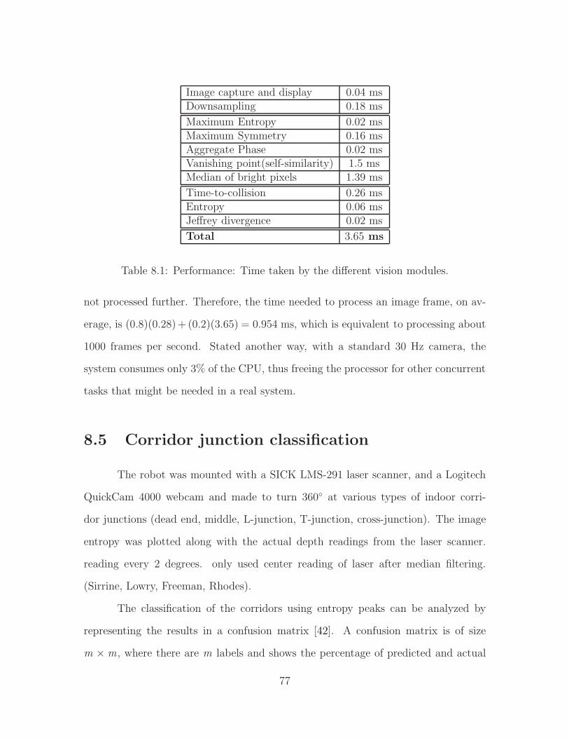
tially and temporally, processing occurs at an average of 1000 frames per second, or

equivalently takes a small fraction of the CPU.

Second, we present an algorithm using image entropy to detect and classify

corridor junctions from low resolution images. Because entropy can be used to per-

ceive depth, it can be used to detect an open corridor in a set of images recorded

by turning a robot at a junction by 360 degrees. Our algorithm involves detecting

peaks from continuously measured entropy values and determining the angular dis-

tance between the detected peaks to determine the type of junction that was recorded

(either middle, L-junction, T-junction, dead-end, or cross junction). We show that

the same algorithm can be used to detect open corridors from both monocular as well

as omnidirectional images.

Third, we propose a minimalistic corridor representation consisting of the ori-

entation line (center) and the wall-floor boundaries (lateral limit). The representa-

tion is extracted from low-resolution images using a novel combination of information

theoretic measures and gradient cues. Our study investigates the impact of image

resolution upon the accuracy of extracting such a geometry, showing that centerline

and wall-floor boundaries can be estimated with reasonable accuracy even in texture-

poor environments with low-resolution images. In a database of 7 unique corridor

sequences for orientation measurements, less than 2% additional error was observed

as the resolution of the image decreased by 99.9%.

iii

Dedication

This work is dedicated to all the researchers and scientists who have inspired

me all my life to ask questions and be persistent.

iv

Acknowledgments

The first thanks must go to my adviser Dr Stan Birchfield, who has been a wall

of support throughout. His patience and foresight have incessantly steered me in the

right direction while saving me from numerous pitfalls. He has taught us equanimity,

fortitude, perseverance and his teachings will be a positive influence in my life for

ever. I must thank Dr Adam Hoover and Dr Ian Walker for teaching me all the

important things early on and Dr Keith Green for introducing me to the creative

side of robotics in architecture. I also thank them for being on the committee and

for their help in directing the research to a credible conclusion by their continuous

positive guidance.

I sincerely thank Dr Rick Tyrrell from the Department of Psychology for the

research discussions with Dr Stan Birchfield, that introduced us to the influential

work by H.W. Leibowitz, that forms the motivation for our work on low-resolution

vision.

I thank Dr Andrew Duchowski of the Computer Science department for giving

me an opportunity to work in the exciting field of eye-tracking and for granting us

permission to use the Tobii eye-tracking equipment.

My fellow research group mates and seniors Zhichao Chen, Neeraj Kanhere,

Shrinivas Pundlik and Guang Zeng, have been very kind to me throughout and have

helped me in various ways to accomplish my research goals.

v

I particularly thank fellow lab-mates Bryan Willimon and Yinxiao Li for all

the research collaborations and the fun discussions we had on robotics and vision. I

also thank Anthony Threatt and Joe Manganelli of the Architecture department for

teaching me many things during our collaborative efforts for Architectural Robotics

class.

Thanks to all the people who helped develop Blepo — the computer vision

library in our department. It made all the code possible.

I extend my gratitude to all the researchers and students of robotics and vision

whose work has influenced and inspired me to start on this venture, without whom

this work would not have been possible.

I must extend my gratitude to National Institute of Medical Informatics for

their generous Ph.D Fellowship and to the Department of Electrical and Computer

Engineering at Clemson for their graduate assistantships throughout my degree pro-

gram.

I thank Lane Swanson and Elizabeth Gibisch for handling all my graduate

paperwork, keeping track of my student status and my assistantships with inimitable

patience.

I thank my friends Shubhada, Divina, Salil, Trupti, Ninad, Sumod and Rahul

for being there with me through these years. I had a wonderful time at Clemson,

mainly due to their unwavering support and friendship.

I thank the elders in the family for being supportive of my decisions and for

their blessings and for being there for me at all times. I also thank the young ones

for bringing cheer and laughter into my life.

Most of all, I thank my wonderful husband Ashwin, for giving me love and

encouragement when I needed it and for being a wall of support in my life.

vi

Table of Contents

Title Page . . . . . . . . . . . . . . . . . . . . . . . . . . . . . . . . . . . i

Abstract . . . . . . . . . . . . . . . . . . . . . . . . . . . . . . . . . . . . ii

Abstract . . . . . . . . . . . . . . . . . . . . . . . . . . . . . . . . . . . . ii

Dedication . . . . . . . . . . . . . . . . . . . . . . . . . . . . . . . . . . . iv

Acknowledgments . . . . . . . . . . . . . . . . . . . . . . . . . . . . . . . v

List of Tables . . . . . . . . . . . . . . . . . . . . . . . . . . . . . . . . . ix

List of Figures . . . . . . . . . . . . . . . . . . . . . . . . . . . . . . . . . x

1 Introduction . . . . . . . . . . . . . . . . . . . . . . . . . . . . . . . . 11.1 Low resolution vision . . . . . . . . . . . . . . . . . . . . . . . . . . . 11.2 The three problems . . . . . . . . . . . . . . . . . . . . . . . . . . . . 31.3 Monocular vision as the sensor . . . . . . . . . . . . . . . . . . . . . . 51.4 What resolution is needed? . . . . . . . . . . . . . . . . . . . . . . . . 61.5 Outline of this dissertation . . . . . . . . . . . . . . . . . . . . . . . . 9

2 Previous Work . . . . . . . . . . . . . . . . . . . . . . . . . . . . . . . 122.1 Low-resolution vision . . . . . . . . . . . . . . . . . . . . . . . . . . . 122.2 Vision based navigation – an overview . . . . . . . . . . . . . . . . . 16

3 Estimating the Orientation in a Corridor . . . . . . . . . . . . . . . 213.1 Entropy . . . . . . . . . . . . . . . . . . . . . . . . . . . . . . . . . . 213.2 Symmetry by mutual information . . . . . . . . . . . . . . . . . . . . 243.3 Aggregate phase . . . . . . . . . . . . . . . . . . . . . . . . . . . . . . 253.4 Vanishing point using self-similarity . . . . . . . . . . . . . . . . . . . 263.5 Median of bright pixels . . . . . . . . . . . . . . . . . . . . . . . . . . 28

4 Estimating the Distance to the End of a Corridor . . . . . . . . . . 304.1 Time-to-collision . . . . . . . . . . . . . . . . . . . . . . . . . . . . . 304.2 Jeffrey divergence . . . . . . . . . . . . . . . . . . . . . . . . . . . . . 31

vii

4.3 Entropy . . . . . . . . . . . . . . . . . . . . . . . . . . . . . . . . . . 32

5 Filtering the estimates using a Kalman filter . . . . . . . . . . . . . 335.1 Noise model development . . . . . . . . . . . . . . . . . . . . . . . . . 335.2 State space variables and parameters for the Kalman filter . . . . . . 425.3 Kalman filter in operation . . . . . . . . . . . . . . . . . . . . . . . . 45

6 Corridor Junction Classification . . . . . . . . . . . . . . . . . . . . 506.1 Junction classification from monocular images . . . . . . . . . . . . . 506.2 Junction classification from omnidirectional images . . . . . . . . . . 54

7 Estimating Corridor Geometry for Navigation . . . . . . . . . . . . 587.1 Minimalistic corridor geometry . . . . . . . . . . . . . . . . . . . . . 587.2 Minimalistic corridor reconstruction . . . . . . . . . . . . . . . . . . . 62

8 Experimental Results . . . . . . . . . . . . . . . . . . . . . . . . . . . 668.1 Orientation along the corridor . . . . . . . . . . . . . . . . . . . . . . 668.2 Distance to the end of the corridor . . . . . . . . . . . . . . . . . . . 688.3 Exploration in an unknown environment . . . . . . . . . . . . . . . . 728.4 Computational efficiency . . . . . . . . . . . . . . . . . . . . . . . . . 758.5 Corridor junction classification . . . . . . . . . . . . . . . . . . . . . . 778.6 Minimalistic corridor representation and reconstruction . . . . . . . . 79

9 Conclusion . . . . . . . . . . . . . . . . . . . . . . . . . . . . . . . . . 889.1 Contributions . . . . . . . . . . . . . . . . . . . . . . . . . . . . . . . 899.2 Future work . . . . . . . . . . . . . . . . . . . . . . . . . . . . . . . . 91

Appendices . . . . . . . . . . . . . . . . . . . . . . . . . . . . . . . . . . . 93

A Time-to-contact Relative to a Planar Surface . . . . . . . . . . . . 94

B Kalman Filter . . . . . . . . . . . . . . . . . . . . . . . . . . . . . . . 99B.1 Kalman filter, matrix notation . . . . . . . . . . . . . . . . . . . . . . 100B.2 Kalman filter in operation . . . . . . . . . . . . . . . . . . . . . . . . 102

C Visual Detection of Light Sources . . . . . . . . . . . . . . . . . . . 104

Bibliography . . . . . . . . . . . . . . . . . . . . . . . . . . . . . . . . . . 106

viii

List of Tables

5.1 Parameter values for the Kalman filter . . . . . . . . . . . . . . . . . 46

8.1 Performance: Time taken by the different vision modules. . . . . . . . 778.2 ROC from confusion matrix . . . . . . . . . . . . . . . . . . . . . . . 788.3 Confusion matrix for corridor classification . . . . . . . . . . . . . . . 79

ix

List of Figures

1.1 A typical corridor image at seven different resolutions . . . . . . . . . 31.2 A typical corridor shown at different image resolutions . . . . . . . . 71.3 Plots of entropy versus image resolution for four different scene types 81.4 k-means segmentation across resolutions . . . . . . . . . . . . . . . . 91.5 The variation of k-means (segmentation) over image resolution . . . . 10

2.1 A taxonomy of approaches to vision-based navigation . . . . . . . . . 17

3.1 Column in image with maximum entropy . . . . . . . . . . . . . . . . 233.2 Gradient phase vectors overlaid on corridor images . . . . . . . . . . 263.3 Vanishing point estimation from global self-similarity . . . . . . . . . 273.4 Comparison between vanishing point estimation techniques . . . . . . 283.5 K-means segmentation results for ceiling lights . . . . . . . . . . . . . 29

5.1 Noise model for median of ceiling lights . . . . . . . . . . . . . . . . . 365.2 Noise model for maximum entropy . . . . . . . . . . . . . . . . . . . 375.3 Noise model for maximum symmetry . . . . . . . . . . . . . . . . . . 385.4 Noise model for vanishing point . . . . . . . . . . . . . . . . . . . . . 395.5 Noise model for aggregate phase . . . . . . . . . . . . . . . . . . . . . 405.6 Noise model for distance to end parameters . . . . . . . . . . . . . . . 415.7 Orientation estimation using the Kalman filter . . . . . . . . . . . . . 485.8 Distance to the end estimation using the Kalman filter . . . . . . . . 49

6.1 Corridor junctions using entropy . . . . . . . . . . . . . . . . . . . . . 516.2 Corridor junction classification . . . . . . . . . . . . . . . . . . . . . . 536.3 1-D panaromic stack and entropy . . . . . . . . . . . . . . . . . . . . 556.4 Sample i=omnidirectional images . . . . . . . . . . . . . . . . . . . . 566.5 Corridor junctions using entropy in omnidirectional images . . . . . . 57

7.1 Ullman local contrast criterion . . . . . . . . . . . . . . . . . . . . . . 607.2 Orientation line estimation . . . . . . . . . . . . . . . . . . . . . . . . 617.3 Homography between image plane and top down view of corridor . . 637.4 Wall-floor boundary and corridor geometric representation . . . . . . 65

8.1 Buildings for orientation test data . . . . . . . . . . . . . . . . . . . . 67

x

8.2 Estimating the center of the corridor using various cues . . . . . . . . 698.3 Sample images from the orientation estimation in one corridor . . . . 708.4 Orientation estimation from 5 measures . . . . . . . . . . . . . . . . . 708.5 Distance to end estimate from 3 measures . . . . . . . . . . . . . . . 718.6 Exploration experiments for ten different corridors . . . . . . . . . . . 748.7 Problematic Corridors . . . . . . . . . . . . . . . . . . . . . . . . . . 758.8 Rapid perception for three different corridors . . . . . . . . . . . . . . 768.9 ROC curve for corridor classification . . . . . . . . . . . . . . . . . . 798.10 Mean error for orientation estimation . . . . . . . . . . . . . . . . . . 818.11 Comparison of results with Kong et al. . . . . . . . . . . . . . . . . . 828.12 Additional results for other corridors . . . . . . . . . . . . . . . . . . 838.13 Corridor structure reconstruction from the wall-floor boundary . . . . 858.14 Mean error for lateral position and width estimation . . . . . . . . . . 868.15 minimalistic representation in 4 resolutions . . . . . . . . . . . . . . . 87

A.1 Perspective projection. . . . . . . . . . . . . . . . . . . . . . . . . . . 95A.2 Camera motion . . . . . . . . . . . . . . . . . . . . . . . . . . . . . . 97

xi

Chapter 1

Introduction

1.1 Low resolution vision

It has been known for some time that natural visual systems contain parallel

pathways for recognition and guidance [100, 94, 77]. While recognition capabilities

deteriorate severely under poor visual conditions such as low-resolution or low illumi-

nation, guidance capabilities remain largely intact. Studying the behavior of human

drivers under adverse conditions, Leibowitz et al. [48, 69, 11] proposed the “selective

degradation hypothesis” to explain the fact that some visual abilities such as vehi-

cle steering and speed control remain relatively easy despite significant loss in visual

acuity and color vision. Their psychovisual experiments revealed that the subjective

magnitude of vection (that is, the vivid sensation of self-motion induced by optical

flow in the visual field) is unaffected by reductions of luminance of eight orders of

magnitude and by refractive errors of up to 20 diopters. In contrast, virtually all

aspects of focal vision (e.g., visual acuity, peak contrast sensitivity, and accommoda-

tion) deteriorate rapidly when light levels drop from daytime to night. Therefore, it

seems plausible that artificial robotic systems should be capable of solving guidance

1

tasks such as exploration and navigation even with impoverished sensing.

In related research, Schneider [2] showed that animals with poor vision were

able to orient themselves toward salient visual events. This research not only con-

firms the use of low resolution sensor data but also highlights a specific application,

namely, detecting salient regions in the visual field. Similarly, we envision mobile

robotic systems that automatically orient themselves toward visually salient regions

(or locations) using low-resolution images. For example, a mobile robot could mea-

sure the image entropy (as an information theoretic measure of saliency) in order to

orient itself toward an open corridor (the salient region).

Furthermore, psychological studies have shown that a human’s gaze while

driving or walking is determined largely by minimalistic information from the envi-

ronment. More specifically, people tend to focus their eye gaze on the direction of

the goal and also along bend points (tangent points) in curved roadways [102, 47].

Therefore, in indoor corridor environments we expect a minimalistic representation

(consisting of vanishing points and wall-floor boundaries) to be sufficient for mobile

robot navigation.

There has also been psychological and artistic perception of low-resolution vi-

sion, in which low-resolution movies are produced using very few LEDs (pixelated

representation).1 Even though the individual objects are not discernible at that reso-

lution, the human visual system is able to fill in gaps in the abstract data [24], making

the moving image perceivable. Such work validates the concept of low-resolution im-

agery.

1http://www.jimcampbell.tv/portfolio/low resolution works/

2

320x240 160x120 80x60 64x48

32x24 16x12 8x6

Figure 1.1: A typical corridor image at seven different resolutions. Even in resolutionsas low as 32 × 24, it is easy to recognize the structure of the corridor. For displaypurposes, the downsampled images we resized so that all of the images are shown inthe same size.

1.2 The three problems

Motivated by these psychological studies, we present solutions to three prob-

lems. First we present an algorithm for estimating the robot’s orientation in the

corridor along with its distance to the end of the corridor to enable autonomous

exploration in a typical unknown indoor environment. Our solution combines a num-

ber of complementary information theoretic measures obtained from low-resolution

grayscale images. After describing these individual measures, we present an inte-

grated system that is able to autonomously explore an unknown indoor environment,

recovering from difficult situations like corners, blank walls, and initial heading to-

ward a wall. All of this behavior is accomplished at a rate of 1000 Hz on a standard

computer using only 0.02% of the information available from a standard color VGA

(640× 480) video camera, discarding 99.98% of the information.

Second, we present a simple peak detection algorithm using a mixture of Gaus-

sians to detect and classify corridor junctions from forward facing monocular as well

3

as omnidirectional images. We show that entropy alone as a measure is enough to

detect open corridors even at a resolution as low as 32 × 24. We present an analy-

sis of the relationship between image entropy and depth of a corridor in an indoor

environment. The spatial property of entropy can be used to give a description of

corridor depth that has direct applications in autonomous corridor navigation using

monocular vision.

Third, we propose a minimalistic representation of a corridor using three lines

that capture the center of the corridor, the left wall-floor boundary, and the right

wall-floor boundary — the intersection of the orientation (center) line with the wall-

floor boundary detected is the vanishing point. We combine ceiling lights with other

metrics such as maximum entropy and maximum symmetry to estimate the center

of the corridor when ceiling lights are not visible. We also introduce the use of

a measure of local contrast in pixels as explained by Ullman [95] for reducing the

effect of specular reflections off the floor and walls. In our experiments, we present

data to establish the best resolution for a mobile robot to explore an indoor corridor,

considering the accuracy and time efficiency. Although higher resolutions may provide

richer information like door frames and sign recognition, which can be used for scene

interpretation, they are not necessary for basic robot navigation tasks.

For all three problems, we use low-resolution 32 × 24 grayscale images. For

all results, we simply downsample the image without smoothing, which decreases

computation time significantly by avoiding touching every pixel. Although there

are good theoretical reasons to smooth before downsampling, we adopt this extreme

approach to test the limits of such an idea. From the example in Figure 1.1, it can be

seen that the discernible elements of a corridor that enable recognition remain fairly

consistent across resolutions until 32× 24.

Why study low resolution? First, the reduced amount of data available leads to

4

greatly reduced processing times, which can be used either to facilitate the use of low-

cost, low-power embedded processors, or to free up the processor to spend more cycles

on higher-level focal vision tasks such as recognition. Secondly, the impoverished

sensor necessarily limits the variety of algorithms that can be applied, thus providing

focus and faster convergence to the research endeavor. Finally, by restricting ourselves

to such impoverished sensory data, it is possible to make quantitative claims about

how much information is needed to accomplish a given task.

1.3 Monocular vision as the sensor

Vision is potentially more informative than other sensors because vision pro-

vides different kinds of information about the environment, while other sensors (such

as sonars or lasers) only provide depth. For landmark detection and recognition,

vision provides direct ways to do so and is easy to represent because of the close

relation to the way humans understand landmarks. In addition lasers are expensive

and power-hungry, and sonars cause interference.

Navigating with a single camera is not easy. Perhaps this is why many ap-

proaches rely upon depth measurements from sonars, lasers, or stereo cameras to solve

the problem. Granted, knowledge of distances to either wall, the shape of obstacles,

and so on, would be directly useful for localizing the robot and building a geomet-

ric map of the environment. Stereo vision has its own difficulties (e.g., it requires

texture to compute correspondence, is computationally expensive and produces inac-

curate results for many pixels). Indoor environments in particular often lack texture,

rendering stereo matching an elusive problem in such places. In contrast, humans are

quite good at navigating indoors with one eye closed, even with blurry vision, thus

motivating us to find a different solution.

5

1.4 What resolution is needed?

1.4.1 Information content in an image

To get a sense of the visible content in a typical corridor image, Fig. 1.2 shows

an example image at successively downsampled resolutions. It can be seen that as the

image is decreased in size from 640×480 to 32×24, the corridor remains recognizable.

However, at the resolution of 16× 12, a noticeable drop in recognizability occurs, in

which it is difficult to discern that the image is of a corridor at all. This observation is

confirmed by noting that the Fourier coefficients are dominated by the low-frequency

terms.

To quantify these results, let I : Ω → V be a grayscale image, where x =

(x , y) ∈ Ω ⊂ R2 are the coordinates of a pixel in the image plane, v ∈ V = 0, . . . , 2n−

1 is a scalar intensity value, and n is the number of bits per pixel. If we assume that

the pixel values in the image were drawn independently according to the probability

mass function (PMF) p(v), then we can say that

H (V ; I ) =∑

v∈V

−p(v)log p(v), (1.1)

is a measure of the information content in the image, where H (V ; I ) is the entropy1 of

a random variable V with PMF p(v). Typically p(v) is estimated by the normalized

graylevel histogram of the image. The entropy of an image is a scalar representing

the statistical measure of randomness that can be used to characterize its texture.

According to Shannon’s theory of entropy [82], the entropy is the measure of infor-

mation content of a random variable and the rarer the random variable’s occurrence

1Note that by the term entropy, we mean the quantity defined according to information theory.Other definitions of entropy, such as those used in thermodynamics or other fields, are not relevantto this work.

6

640× 480 128× 96 64× 48 32× 24 16× 12

Figure 1.2: Top: A typical corridor shown at different image resolutions. As theimage resolution drops from 640× 480 to 32× 24, the pattern of the corridor is stillobservable, but at 16× 12 it is difficult to recognize the scene at all. Bottom: Thecorresponding Fourier coefficients (logarithmic display) show that the low frequencycoefficients are more prominent.

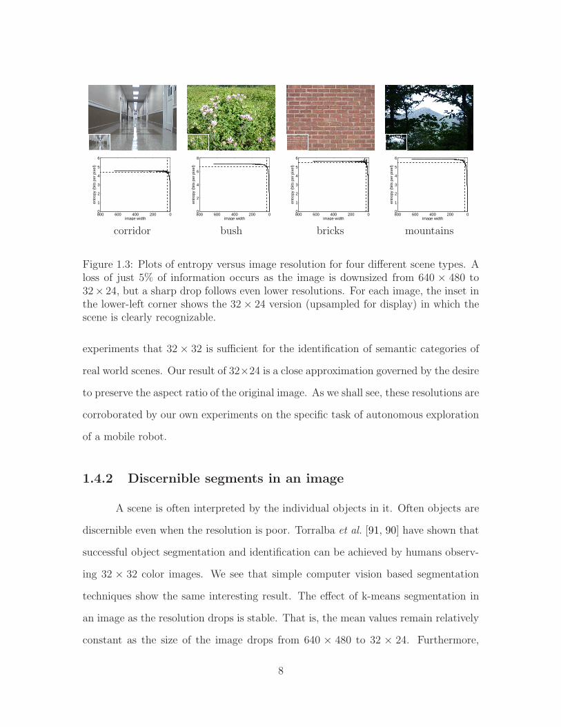
the greater the information content of the random variable. Fig. 1.3 shows that for a

variety of environments, the entropy of an image does not change significantly as the

image is downsized from 640×480 to 32×24. In fact, at the latter resolution, there is

only a 5% drop in entropy from the original image. However, as the resolution drops

below 32× 24, the entropy drops sharply.

Of course, the entropy of the random variable associated with the graylevel

values of the pixels in an image is not the only way to measure information content.

As a result, this experiment does not necessarily establish any validity to the claim

that for any given task such a resolution is sufficient. However, we argue that there is

a close connection between the coarse information needed for autonomous guidance

(whether exploration or navigation) of a mobile robot and the more general problem of

scene recognition. In both cases, the task is aimed at gleaning summary information

from the entire image rather than discovering particular identities of objects in the

scene. To this end, it is interesting to note that our results are similar to those

of Torralba and colleagues [90, 91]. Their independent work on determining the

spatial resolution limit for scene recognition has established through psychovisual

7

800 600 400 200 00

1

2

3

4

5

6

image width

entr

opy

(bits

per

pix

el)

800 600 400 200 00

2

4

6

8

image width

entr

opy

(bits

per

pix

el)

800 600 400 200 00

1

2

3

4

5

6

image width

entr

opy

(bits

per

pix

el)

800 600 400 200 00

1

2

3

4

5

6

image width

entr

opy

(bits

per

pix

el)

corridor bush bricks mountains

Figure 1.3: Plots of entropy versus image resolution for four different scene types. Aloss of just 5% of information occurs as the image is downsized from 640 × 480 to32× 24, but a sharp drop follows even lower resolutions. For each image, the inset inthe lower-left corner shows the 32× 24 version (upsampled for display) in which thescene is clearly recognizable.

experiments that 32 × 32 is sufficient for the identification of semantic categories of

real world scenes. Our result of 32×24 is a close approximation governed by the desire

to preserve the aspect ratio of the original image. As we shall see, these resolutions are

corroborated by our own experiments on the specific task of autonomous exploration

of a mobile robot.

1.4.2 Discernible segments in an image

A scene is often interpreted by the individual objects in it. Often objects are

discernible even when the resolution is poor. Torralba et al. [91, 90] have shown that

successful object segmentation and identification can be achieved by humans observ-

ing 32 × 32 color images. We see that simple computer vision based segmentation

techniques show the same interesting result. The effect of k-means segmentation in

an image as the resolution drops is stable. That is, the mean values remain relatively

constant as the size of the image drops from 640 × 480 to 32 × 24. Furthermore,

8

the segments are discernible and distinct even as resolution drops and they begin to

coalesce only after the resolution of 32× 24. See Figures 1.4 and 1.5.

640x480 320x240 160x120 80x60

64x48 32x24 16x12 8x6

Figure 1.4: The figure shows the k-means segmentation results on a typical corridorimage with k=10. It can be seen that the individual segments are discernible andconsistent across resolutions until the resolution of 32×24. For resolutions lower thanthat, the segments begin to merge.

From the above discussions, we can see that there is sufficient evidence from a

number of sources: psychology, independent research by Torralba et al. [90, 91], infor-

mation theoretic measurements on images (entropy) and observing the segmentation

of images across resolutions, that 32×24 seems to be approximately the optimal low-

resolution that is necessary and sufficient for a variety of simple tasks like detection

and recognition. We will show that the same confidence can be extended to robot

navigation/exploration tasks.

1.5 Outline of this dissertation

The next chapter gives a summary of the work done previously in vision based

navigation, the different approaches, the achievements, limitations, and ongoing work.

Chapters 3, 4, 5, and 6 describe the detailed structure of the algorithms, the percepts,

9

640x480 320x240 160x120 80x60 64x48 32x24 16x12 8x6 4x3 2x180

90

100

110

120

130

140

150

image resolution

k−m

eans

640x480 320x240 160x120 80x60 64x48 32x24 16x12 8x6 4x3 2x160

80

100

120

140

160

180

200

image resolution

k−m

eans

k = 2 k = 3

640x480 320x240 160x120 80x60 64x48 32x24 16x12 8x6 4x3 2x160

80

100

120

140

160

180

200

220

240

image resolution

k−m

eans

640x480 320x240 160x120 80x60 64x48 32x24 16x12 8x6 4x3 2x10

50

100

150

200

250

image resolution

k−m

eans

k = 5 k = 10

Figure 1.5: The variation of the mean values for different values of k . It can beseen that when resolution drops, the mean values do not change significantly until32 × 24 after which all means converge rapidly. This highlights that objects in animage retain their composition in general as resolution drops until the approximatelyoptimal size of 32× 24.

10

the visual processing for navigation. Chapter 7 discusses a number of experiments

conducted on the robot in an indoor environment, with supporting plots, graphs and

image sequences. These give us a sense of the reliability of the algorithms and their

limitations. Chapter 8 gives a summary of the dissertation, an outline of future work

and concluding discussions.

11

Chapter 2

Previous Work

2.1 Low-resolution vision

Experiments conducted by Torralba and Sinha [92] have established lower

bounds on image resolution needed for reliable discrimination between face and non-

face patterns, indicating that the human visual system is surprisingly effective at

detecting faces in low resolutions. Similarly, Hayashi and Hasegawa [26] have de-

veloped a method that achieves a face detection rate of 71% for as small as 6 × 6

face patterns extracted from larger images. Torralba et al. [91, 90] in their recent

work have presented several psychovisual experiments to show that 32 × 24 images

are sufficient for human beings to successfully performs basic scene classification,

object segmentation, identification . They have shown results on an extensively con-

structed database of 80 million images that make a powerful argument in favor of

low-resolution vision for non-parametric object and scene recognition. The applica-

tion to person detection and localization is particularly noteworthy considering that

they have produced good results with low-resolution images that are comparable to

that of the Viola-Jones detector which uses high-resolution images. The whole spirit

12

of low-resolution is strengthened by this argument and one can see that low-resolution

images provide enough information for basic visual processing. Judd et al. [34] con-

ducted psycho-visual experiments to investigate how image resolution affects fixation

locations and consistency across humans through an eye-tracking experiment. They

found that fixations from lower resolution images can predict fixations on higher res-

olution images, that human fixations are biased toward the center for all resolutions,

and this bias is stronger at lower resolutions. Furthermore they found that human fix-

ations become more consistent as resolution increases until around 16-64 pixels (1/2

to 2 cycles per degree) after which consistency remains relatively constant despite the

spread of fixations away from the center. Here again the work shows interestingly

consistent results at image resolutions 32× 32.

There is a connection between low-resolution vision and the notion of scale

space [103, 50]. Scale space processing emphasizes extracting information from mul-

tiple scales and is the basis of popular feature detection algorithms such as SIFT [52]

and SURF [5]. Koenderink [40] speaks of the “deep structure” within images, arguing

that human visual system perceives images at several levels of resolution simultane-

ously. His distinction between deep and superficial structure is closely related to the

distinction between focal (for recognition) and ambient (for guidance) vision [100].

There is also a recent emphasis on minimalistic sensing. Tovar et al. [93]

in their recent work have developed an advanced data structure for constructing a

minimal representation based entirely on critical events in online sensor measure-

ments made by the robot. The goal was to enable mobile robotic systems to perform

sophisticated visibility-based tasks with minimal sensing requirements. Because pre-

vious algorithmic efforts like SLAM often assume the availability of perfect geometric

models, they are susceptible to problems such as mapping uncertainty, registration,

segmentation, localization and control errors. In their work, depth discontinuities

13

are encoded in a simple data structure called the Gap Navigation Tree (GNT) which

evolves over time from online sensor measurements (two laser range sensors), to pro-

vide the robot the shortest path to the goal. O’Kane and LaValle in their work [68]

have described an ‘almost-sensorless localization’ system, using only a compass, a

contact sensor and a map of the environment. Because no odometry is available,

the robot can only make make maximal linear motions in a chosen direction in an

environment till the limits. The history of such actions is also available to the robot.

They have shown that a simple system like this is actually capable of localization.

There has also been an emphasis on ‘lightweight’ or ‘low-feature’ SLAM tech-

niques with the goal of reducing the computational burden in embedded robotic sys-

tems. Nguyen et al. [67] have developed a system that performs lightweight SLAM, an

algorithm that uses only perpendicular or parallel lines in the environment for map-

ping because they represent the main structure of most of the indoor environments.

By using orthogonality as a geometric constraint in the environment, many unwanted

dynamic objects are removed in the desired reconstruction leading to a rather precise

and consistent mapping. This is synonymous with the spirit of downsampling an

image to remove noise/reflections. Choi et al. [16] have also developed a line-feature

based SLAM in a geometrically constrained extended Kalman filter framework. They

have developed an efficient line extraction algorithm that works on measurements ob-

tained from sparse, low-grade sensors which reduce the search space by representing

the indoor environment using a combination of these line features. They have shown

results in which a room has been modeled using the geometry of the room as well as

rectangular objects present in the room. Localization is shown to be achieved with

good accuracy even with impoverished sensor information.

Representation of indoor environments has largely been geometric. While

previous studies suggest that humans rely on geometric visual information (hallway

14

structure) rather than non-geometric visual information (e.g., doors, signs and light-

ing) for acquiring cognitive maps of novel indoor layouts, Kalia et al. [35] in their

recent work have shown that humans rely on both geometric and non-geometric cues

under constraints of low-vision.

Vision-based mobile robot navigation has been studied by many researchers.

From the early work of the Stanford Cart [63] to the current Aibo (the toy robot

built by Sony), navigation has been recognized as a fundamental capability that

needs to be developed. According to the survey of DeSouza et al. [22], significant

achievements have been made in indoor navigation, with FINALE [45] being one of the

more successful systems. FINALE requires a model-based geometric representation

of the environment and uses ultrasonic sensors for obstacle avoidance. NEURO-

NAV [59] is another oft cited system that uses a topological representation of the

environment and responds to human-like commands. RHINO [12] is an example of a

robust indoor navigating robot. The highly notable NAVLAB [88] is an example of

proficient outdoor navigation system which use a combination of vision and a variety

of other sensors for navigation and obstacle avoidance. Moravec [63] and Nelson et

al. [66], however, have emphasized the importance of low-level vision in mobile robot

navigation, and Horswill [30] implemented a hierarchical and complete end-to-end

vision-based navigational robot based on prior training of the environment.

Historically, low-resolution images have been used for various mobile robotic

tasks because of the limitations of processing speeds. For example, in developing

a tour-giving autonomous navigating robot, Horswill [31] used 64 × 48 images for

navigation and 16 × 12 images for place recognition. Similarly, the ALVINN neural

network controlled the autonomous CMU NAVLAB using just 30 × 32 images as

input [70]. Robust obstacle avoidance was achieved by Lorigo et al. [51] using 64×48

images. In contrast to this historical work, our approach is driven not by hardware

15

limitations by rather inspired by the limits of possibility, as in Torralba et al. [91,

92] and in Basu and Li [4], who argue that different resolutions should be used for

different robotic tasks. Our work is unique in that we demonstrate autonomous

navigation in unknown indoor environments using not only low-resolution images but

also intermittent processing.

2.2 Vision based navigation – an overview

Typically using on-board computation and standard off the shelf hardware,

mobile robots using multiple sensors have been developed for land, sea and aerial

navigation and are deployed in the manufacturing, military, security, consumer and

entertainment industries. Vision is powerful because it is inexpensive, non-intrusive

and scalable. The various ways in which vision is used for navigation have been

described in detail, by Desouza et al. [22]. Vision-based navigation systems can be

classified as shown in Figure 2.1 which is a summary of [22]. This thesis aims to

form a bridge between map-building systems and mapless systems, thus combining

the goal of autonomous exploration and mapping.

2.2.1 Mapless navigation

Mapless navigation using vision predominantly uses primitive visual compe-

tencies like measurements of 2D motion (such a optical flow), structure from motion,

independent motion detection, estimating time-to-contact and object tracking [22].

While some/all of these can and have been used to develop a wandering robot, many

open points of research need to be mentioned. None of these have been tested before

on low-resolution systems (as low as 32 × 24). All of these visual competencies are

known to face problems in textureless environments. These competencies can be used

16

Figure 2.1: A taxonomy of approaches to vision-based navigation, summarizing [22].

for continuous navigation in a predictable path. At a point of discontinuity such as a

corridor end, however, these competencies themselves do not provide a solution.

2.2.2 Map-based navigation

Map-based navigation systems are a complete solution to the goal-based nav-

igation problem. The definition of landmarks is a vital necessity of such a system.

Again, historically there have been two types of visual landmarks: Sparse feature

based landmarks and higher level abstract landmarks.

• Sparse feature based landmarks : Some of the prominent landmarks used today

to represent visual landmarks in SLAM based systems, are based on edges,

rotation invariant features, or corners. These are in fact represented by the

three popular visual landmark representation techniques: SIFT (Scale Invariant

Feature Transform) [79], Harris Corners [25] or Shi-Tomasi feature points [84].

These have the advantage of being robust, scale invariant and sparse [39]. But

again the important points to be noted are as follows. These representations

17

are computationally quite expensive. Some work has been done to develop real-

time feature detectors, like real-time SLAM [21], GLOH [60] and SURF [6].

FAST [74, 75] is promising for high-speed, feature-based representations, but

such approaches often leave little CPU time for other tasks and may not work

well with textureless environments. These features work well in well-textured

environments with high-resolution. In poorly textured environments with low

resolution, sparse features are not robust enough. SIFT in particular is fairly

sensitive to resolution and texture.

• High level abstract landmarks : Another way of representing landmarks is to use

all of the pixels together like the entire image itself, or reduced pixel information.

Template matching is a very simple, common yet powerful landmarks represen-

tation/matching technique. Histograms, color maps and other measures are

also popular.

2.2.3 SLAM: Simultaneous Localization and Mapping

With regard to mapping, the recent developments in Simultaneous Localiza-

tion and Mapping (SLAM) have been based primarily upon the use of range sensors

[62, 72, 9]. A few researchers have applied this work to the problem of building maps

using monocular cameras, such as in the vSLAM approach [37], which is a software

platform for visual mapping and localization using sparse visual features. An alter-

nate approach is that of Davison et al. [20, 19], who also use sparse image features to

build 3D geometric maps.

In these visual SLAM techniques, either a complex matching process for a

simple landmark representation [73] or a simple matching process for a complex land-

mark representation [79] is needed for robust robot localization. In indoor corridor

18

environments, however, the lack of texture poses a major obstacle to such an ap-

proach. Indeed, popular techniques such as the Scale Invariant Feature Transform

(SIFT) [79] or other feature representations have difficulty in such cases. Moreover,

the computationally demanding nature of these algorithms often leaves little room

for additional processing, and their design requires higher resolution images.

2.2.4 Map-building based navigation

The whole task of map-building described in modern SLAM, visual or not,

always has a manual/tele-operated phase [18, 78, 20]. It is important to note that in

most map-building systems, the robot is controlled manually. Autonomous naviga-

tion is rare, and autonomous vision-based mapping is even more rare [22]. Notable

initiatives include the work done by Matsumoto et al. [55], who used omnidirectional

cameras with stereo and optical flow to control navigation, and Shah et al. [81],

who implemented an autonomous navigation system using a calibrated fish eye stereo

lens system. However, these approaches require specialized cameras. Similarly, au-

tonomous vision-based navigation is rare, with many techniques requiring a training

phase in which the robot is controlled manually [8, 13, 56, 57, 33]. As a result, efficient

autonomous map building of indoor environments using a single off-the-shelf camera

has remained an elusive problem.

Team ARobAS of INRIA have made a compelling statement in their annual

report [87] about the incompleteness of SLAM. They state that the problem of explo-

rative motion strategy of the robot (or reactive navigation) has rarely been a part of

SLAM. They argue that autonomous navigation and SLAM cannot be treated sepa-

rately and that a unified framework is needed for perception, modeling and control.

Very few notable initiatives have completely automated the system for collecting the

19

data required to build a map while navigating. Robust perception is a basic neces-

sity for a navigating robot that can be deployed in an environment without human

intervention.

It is also important to distinguish our work from the large body of SLAM

literature [89]. Simultaneous localization and mapping (SLAM) aims to produce a

map of the environment while at the same time determining the robot’s location

within the map. Such approaches do not typically focus on autonomous exploration.

One notable exception is the RatSLAM system [61], which is capable of robust au-

tonomous exploration, mapping, localization, and navigation using a combination of

vision, laser, sonar, and odometry sensors. RatSLAM is inspired by biological systems

which demonstrate the ability to build and maintain spatial representations that are

used as the basis of goal directed navigation throughout the lifetime of the organism.

The localization and mapping algorithm is based on computational models of parts

of the rodent’s brain. The system built was a mobile robotic platform that is capable

of mock delivery tasks in an office building. However even though vision is used in

the mapping process, only lasers, sonars, and odometry are used to aid autonomous

navigation around obstacles and straight line navigation. In contrast, our approach

achieves more modest objectives but relies on vision alone.

20

Chapter 3

Estimating the Orientation in a

Corridor

In order for a mobile robot to autonomously maneuver through an indoor

office environment, one obvious parameter that must be estimated is the robot’s

orientation within the corridor. We propose to combine five complementary ways

of estimating this value from low-resolution images: the entropy of the image, the

symmetry as measured by mutual information, aggregate phase, vanishing points

using self-similarity of the image, and the median of the bright pixels. The goal is

to learn a mapping f : I → θ, where I is the low-resolution image and θ is the

orientation of the robot with respect the primary axis of the corridor.

3.1 Entropy

We have found empirically that, as a general rule, entropy is maximum when

the camera is pointing down the corridor. The reason for this (perhaps surprising)

result is that such an orientation causes scene surfaces from a variety of depths to

21

be visible, yielding an increase of image information at this orientation. In contrast,

when the robot is turned so that it faces one of the side walls, the range of visible

depths is much smaller and therefore the variety of pixel intensities usually decreases.

A similar observation has been noted by other researchers in the context of using

omnidirectional images [10, 23], but we show that the relationship between entropy

and orientation holds even for standard camera geometries. In addition, we have

found that the relationship is not significantly affected whether or not the walls are

textured.

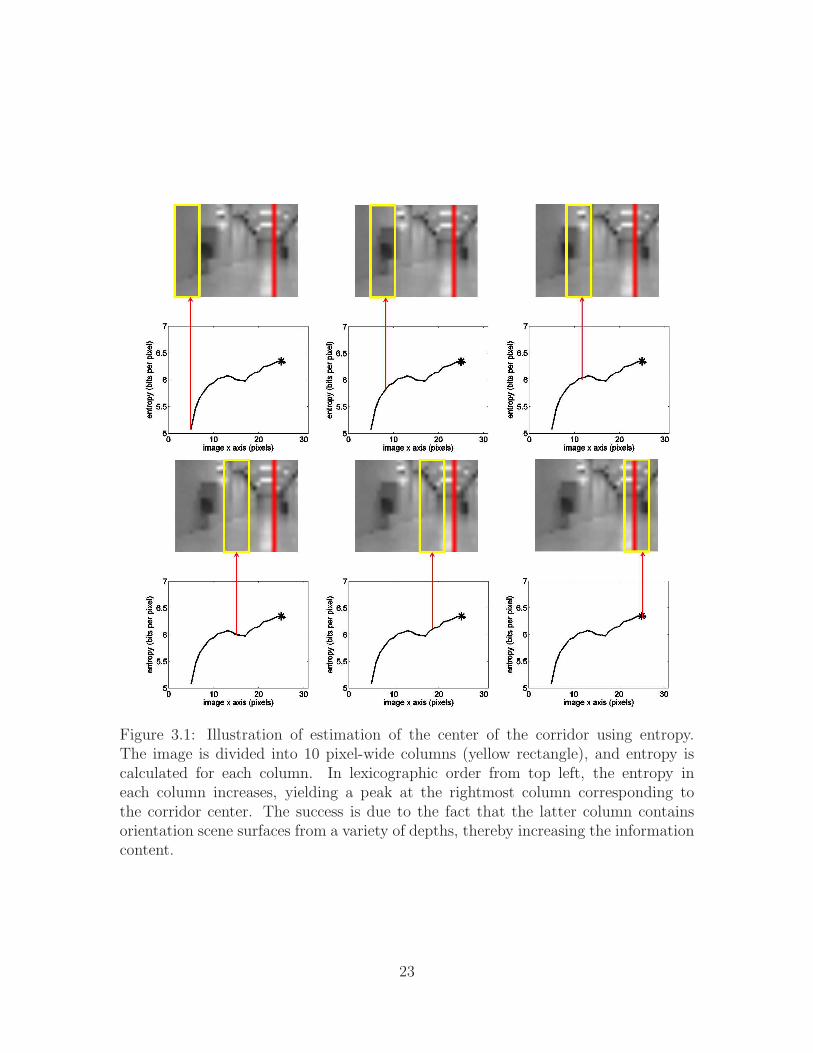
We exploit this property by dividing the image into overlapping vertical slices

and computing the graylevel entropy of the image pixels in each slice. The hor-

izontal coordinate yielding the maximum entropy is then an estimate of the ori-

entation. More precisely, let us define a vertical slice of pixels centered at x as

Cω(x ) = (x ′, y ′) : ω2≤| x − x ′ |< ω

2, where ω is the width of the slice. If p(v ; x ) is

the normalized histogram of pixel values in Cω(x ), then the graylevel entropy of the

slice is given by H (V ; I , x ) = −∑

v∈V p(v ; x ) log p(v ; x ). This is illustrated in Fig-

ure 3.1. The orientation estimate is then given by f1(I ) = ψ(argmaxx H (V ; I , x )),

where the function ψ converts from pixels to degrees. With a flat image sensor and no

lens distortion, the horizontal pixel coordinate is proportional to the tangent of the

angle that the projection ray makes with the optical axis. Since the tangent function

is approximately linear for angles less than 30 degrees, we approximate this trans-

formation by applying a scalar factor: ψ(x ) = αx , where the factor α is determined

empirically.

22

Figure 3.1: Illustration of estimation of the center of the corridor using entropy.The image is divided into 10 pixel-wide columns (yellow rectangle), and entropy iscalculated for each column. In lexicographic order from top left, the entropy ineach column increases, yielding a peak at the rightmost column corresponding tothe corridor center. The success is due to the fact that the latter column containsorientation scene surfaces from a variety of depths, thereby increasing the informationcontent.

23

3.2 Symmetry by mutual information

Symmetry is defined as the invariance of a configuration of elements under a

group of automorphic transformations [101]. However, the exact mathematical def-

inition is inadequate to describe and quantify the symmetries found in the natural

world nor those found in the visual world. Zabradosky et al. [104] mention that even

perfectly symmetric objects lose their exact symmetry when projected onto the im-

age plane or the retina due to occlusion, perspective transformations, digitization,

etc. Thus, although symmetry is usually considered a binary feature, (i.e. an ob-

ject is either symmetric or it is not symmetric), we view symmetry as a continuous

feature where intermediate values of symmetry denote some intermediate amount of

symmetry [104]. Much of the work related to symmetry concerns symmetry detection

(symmetry in the binary sense) as in [14, 86, 3, 83]. Very few noteworthy contributions

exist that venture to measure the amount of symmetry in an image. Zabradosky et al.

[104], Marola [54], Kanatani [36], van Gool [97] are some of the prominant authors in

this respect. However all of these experiments associate symmetry with shape, which

requires shape computation/comparison of some kind with respect to a discrete set.

To the best of our knowledge a continuous measure of symmetry using low level image

information (the raw image bits) in low resolution has not been developed before. We

propose a new measure of symmetry using information theoretic clues.

Another property of corridors is that they tend to be symmetric about their

primary axis. Various approaches to detecting and measuring symmetry have been

proposed [104, 46, 3, 14]. However, in our problem domain it is important to measure

the amount of symmetry rather than to simply detect axes of symmetry. One way

to measure the amount of reflective symmetry about an axis is to compare the two

regions on either side of the axis using mutual information. Mutual information is

24

a measure of the amount of information that one random variable contains about

another random variable, or equivalently, it is the reduction in the uncertainty of one

random variable due to the knowledge of the other. Mutual information has emerged

in recent years as an effective similarity measure for comparing images [38, 76, 27]. As

with entropy, for each horizontal coordinate x a column of pixels C(x ) is considered,

where we have dropped the ω subscript for notational simplicity. The column is

divided in half along its vertical center into two columns CL(x ) and CR(x ). The

normalized graylevel histograms of these two regions are used as the two probability

mass functions (PMFs), and the mutual information between the two functions is

computed:

MI (x ) =∑

v∈V

∑

w∈V

p(v ,w ; x ) logp(v ,w ; x )

pL(v ; x )pR(w ; x ), (3.1)

where p(v ,w ; x ) is the joint PMF of the intensities in both sides, and pL(v ; x ) and

pR(w ; x ) are the PMFs computed separately of the intensities of the two sides. As

before, the orientation estimate is given by f2(I ) = ψ(argmaxx MI (x )).

3.3 Aggregate phase

A third property of corridors is that the dominant intensity edges tend to

point down the length of the corridor. Therefore, near the center of the corridor,

the phase angles of these edges on the left and right sides will balance each other,

yielding a small sum when they are added together. We compute the gradient of the

image using a Sobel operator and retain only the phase φ(x , y) of the gradient at each

pixel. For each horizontal coordinate x we simply add the phase angle of all the pixels

in the vertical slice: AP(x ) =∑

(x ,y)∈C(x) φ(x , y). The orientation estimate is given

by f3(I ) = ψ(argminx AP(x )). Phase angles overlaid on several example images are

25

corridor to the left corridor centered corridor to the right

Figure 3.2: Gradient phase vectors overlaid on corridor images. From left to right:The center of the corridor is on the left side of the image, in the center of the image,and on the right side of the image. The phase vectors generally point toward thecenter of the corridor, so that in a vertical stripe near the center, the vectors balanceeach other.

shown in Figure 3.2.

3.4 Vanishing point using self-similarity

An additional property of corridors is the vanishing point, which is nearly

always present in the image when the robot is facing down the corridor. Our approach

is based on the work of Kogan et al. [41], who developed a novel self-similarity based

method for vanishing point estimation in man-made scenes. The key idea of their

approach, based upon the work of Stentiford [85], is that a central vanishing point

(meaning a vanishing point that is visible in the image) corresponds to the point

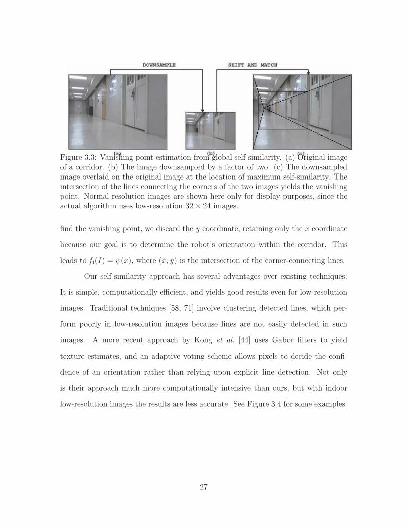
around which the image is locally self similar under scaling changes. See Figure 3.3.

While Kogan et al. [41] use 1D cross-sections of the image for similarity matching

using affine transformation and cross correlation, we instead shift the downsampled

image across the original image and calculate the mutual information between the

two windows. The point at which the mutual information between the two images is

maximum yields a location for the downsampled image. The vanishing point is then

found by intersecting the lines connecting the corners of the two images. Once we

26

Figure 3.3: Vanishing point estimation from global self-similarity. (a) Original imageof a corridor. (b) The image downsampled by a factor of two. (c) The downsampledimage overlaid on the original image at the location of maximum self-similarity. Theintersection of the lines connecting the corners of the two images yields the vanishingpoint. Normal resolution images are shown here only for display purposes, since theactual algorithm uses low-resolution 32× 24 images.

find the vanishing point, we discard the y coordinate, retaining only the x coordinate

because our goal is to determine the robot’s orientation within the corridor. This

leads to f4(I ) = ψ(x ), where (x , y) is the intersection of the corner-connecting lines.

Our self-similarity approach has several advantages over existing techniques:

It is simple, computationally efficient, and yields good results even for low-resolution

images. Traditional techniques [58, 71] involve clustering detected lines, which per-

form poorly in low-resolution images because lines are not easily detected in such

images. A more recent approach by Kong et al. [44] uses Gabor filters to yield

texture estimates, and an adaptive voting scheme allows pixels to decide the confi-

dence of an orientation rather than relying upon explicit line detection. Not only

is their approach much more computationally intensive than ours, but with indoor

low-resolution images the results are less accurate. See Figure 3.4 for some examples.

27

Figure 3.4: Comparison between our vanishing point estimation approach (greencircle) using self-similarity and that of Kong et al. [44] (red plus). Our approach ismore robust to the scenario of low texture information which is common in indoorscenes.

3.5 Median of bright pixels

The ceiling lights, which are usually symmetric with respect to the main cor-

ridor axis, provide another important cue. Due to the low resolution of the image, it

is not possible to analyze the shape of the lights, as in [15]. Moreover, sometimes the

lights are not in the center of the corridor but rather on the sides. A simple technique

that overcomes these difficulties is to apply the k -means algorithm [53] to the graylevel

values in the upper half of the image, with k = 2. The median horizontal position

of the brighter of the two regions is calculated, yielding an estimate of the center of

the corridor. (The use of median as opposed to mean prevents the result from being

affected by specular reflections on either wall.) We have found this approach to be not

only simpler, but also more accurate and more generally applicable, than the shape-

based technique in [15]. Note that ceiling lights provide an added advantage over

vanishing points because they are affected by translation, thus enabling the robot to

remain in the center of the corridor while also aligning its orientation with the walls.

As with the previous measure, the horizontal coordinate is transformed to an angle

by applying the same scalar factor. Therefore, f5(I ) = ψ(medx : (x , y) ∈ Rbright),

where Rbright is the set of bright pixels. Some segmentation results are shown in

Figure 3.5.

28

Figure 3.5: K-means segmentation results for ceiling lights, with k=2 (top), andcorresponding estimate (red vertical line) of the center of the corridor bottom.

29

Chapter 4

Estimating the Distance to the

End of a Corridor

The second state parameter to be estimated is the distance to the end of the

corridor. To solve this problem, we combine three complementary measures: time-

to-collision, Jeffrey divergence, and entropy.

4.1 Time-to-collision

Time-to-collision (TTC) is defined as the time it will take the center of pro-

jection of a camera to reach the opaque surface intersecting the optical axis, if the

relative velocity between the camera and the surface remains constant. Traditional

methods of computing TTC [1, 17] require computing the divergence of the estimated

optical flow, which is not only computationally intensive but, more importantly, re-

quires a significant amount of texture in the scene. To overcome these problems, Horn

et al. [29] have recently described a direct method to determine the time-to-collision

using image brightness derivatives (temporal and spatial) without any calibration,

30

tracking, or optical flow estimation. The method computes the TTC using just two

frames of a sequence, filtering the output using a median filter, to yield a reliable

estimate as the camera approaches the object. This method is particularly applicable

to our scenario in which the robot approaches a planar surface by translating in a

direction parallel to the optical axis, a scenario for which the algorithm achieves an

extremely simple formulation. Given two successive image frames I (1) and I (2) taken

at different times, the TTC is computed as

τ(I (1), I (2)) =−∑

x ,y(G (x , y))2∑

x ,y G (x , y) It(x , y), (4.1)

where G (x , y) = xIx(x , y)+yIy(x , y), Ix and Iy are the spatial derivatives of the image

intensity function, and It(x , y) is the temporal derivative. Normally, the summation

would be computed over the desired planar object, but in our case we compute the

sum over the entire image. Although the scene is not strictly planar when the robot

is at the beginning of the corridor, we have found empirically that the TTC values

are nevertheless higher at the beginning of the corridor, indicating that the method

succeeds in estimate the TTC qualitatively even at larger distances. As the robot

approaches the end of the corridor, the scene in the field of view becomes more

planar, thereby increasing the accuracy of the estimated TTC. We transform the

TTC to an estimate of the distance to the end by dividing the robot speed by it:

g1(I(1), I (2)) = s/τ(I (1), I (2)), where s is the robot translational speed.

4.2 Jeffrey divergence

As the robot approaches the end of the corridor, the pixel velocities increase,

thereby causing the image to change more rapidly. As a result, another way to

31

estimate the distance to the end is to measure the distance between two images. A

convenient way to compare two images is to measure the Jeffrey divergence [96], which

is a symmetric version of the Kullback-Leibler divergence:

J (p, q) =∑

v∈V

(

p(v) log

(

p(v)

q(v)

)

+ q(v) log

(

q(v)

p(v)

))

, (4.2)

where p and q are the graylevel histograms of the two successive images I (1) and

I (2), respectively, and the summations are over the entire image. There is an inverse

relationship between the divergence and the distance, so we transform this value to

an estimate of the distance to the end by subtracting a scaled version from a constant

to keep the result non-negative: g2(I(1), I (2)) = β2 − α2J (p

(1), q (2)), where β2 is the

offset.

4.3 Entropy

It is also true that, as the robot approaches the end of the corridor, the entropy

of the image increases more rapidly. An alternate way to estimate the distance to the

end, then, is to compute the difference in entropy between consecutive image frames,

which also has an inverse relationship with distance: g3(I(1), I (2)) = α3/(H (V ; I (1))−

H (V ; I (2))), where α3 is a scale factor.

32

Chapter 5

Filtering the estimates using a

Kalman filter

In our previous work we estimated orientation using only the median of bright

pixels and distance to the end of the corridor was largely determined by entropy

[64]. In recent work we showed that a linear combination (weighted average) of

five (orientation) and three (distance to the end) complementary measures is more

effective for achieving success in multiple environments [65]. However we now show a

state space representation of the variables to be estimated, namely orientation in the

corridor (θ) and distance to the end (d). We show that a Kalman filter combining

the measurements is most effective in this case, providing more reliable estimates over

time than a simple weighted average.

5.1 Noise model development

In order to reduce the effects of noise that corrupts the measurements from

the image, we need to set up a filter to remove/reduce the noise in the state space

33

represented by orientation in the corridor and the distance to the end of the corridor.

We know that the motion of the robot along a straight line in the corridor is linear

and assuming that the noise is Gaussian, we can use a Kalman filter to achieve robust

state estimation as shown in Appendix 2. Two major statistical properties are studied

to analyze the noise characteristics and evaluate the noise models: the histogram

and the autocorrelation function [32, 98]. Our goal of modeling a sensor system is

to construct a probabilistic model using some commonly used random variables or

processes. Additive White Gaussian Noise (AWGN) is a typical random process for

this scenario. Since techniques relating AWGN are well-developed, analysis would

be simplified if the sensor noise of interest is AWGN or can be approximated as

such. By contrast, if the characteristics exhibited by the data are too complex to be

modeled easily and model accuracy is less important, use of a typical random process

or combinations of several of them are justifiable for rough approximation.

5.1.1 Histogram (estimation of Gaussian probability density

function)

For a given single location, if multiple sensor readings are takes and the mea-

surements are analyzed, the histogram of the residuals of the measurements gives

us an approximation of the probability density of the noise involved. Jenkins et al.

[32] showed that if the histogram approximates a bell shaped curve, then the noise

characteristics can be considered Gaussian.

5.1.2 Sample autocorrelation function (White Noise)

The autocorrelation function describes the second order statistics of a random

process. It is used here because it gives a visual picture of the degree to which samples

34

in the process are dependent upon each other as a function of the separation between

points in the data series. From Jenkins [32], the autocovariance function (ACVF)

estimates of a discrete time series could be defined as following: If the observations

X1, X2, .... Xn are a discrete set of values corresponding to multiple measurements

for the same actual (unobservable) value, the discrete autocovariance estimate is:

cxx (k) =1

N

N−k∑

i=1

(xi − x )(xi+k − x ), k = 0, 1, ...N − 1 (5.1)

where x = 1N

∑N

i=1 xi . Estimates of the autocorrelation function (ACF), also called

sample ACF, are obtainable by dividing the above ACVF estimates by the estimate

of the variance, which is

rxx (k) =cxx (k)

cxx (0)(5.2)

The ACF of an ideal white Gaussian process is always zero. So ACF of a set

of residual test data which settle down at zero or are close to zero can be considered/-

modeled as white Gaussian noise.

5.1.3 Noise model for orientation measurements

We estimate the noise model for the five orientation measurements, median of

ceiling lights, maximum entropy, maximum symmetry, vanishing points and aggregate

phase. In each case we show that the histogram of the residual noise for a few token

well separated orientation measurements closely match the Gaussian. We also show

that the ACF approaches zero in each case, establishing the noise in each case to be

AWGN.

35

−20 −15 −10 −5 0 50

2

4

6

8

10

residual values (pixels)

no o

f sam

ples

−20 −10 0 10 200

5

10

15

20


no o

f sam

ples

−10 0 10 200

5

10

15


no o

f sam

ples

0 10 20 30 40 50−20

−15

−10

−5

0

5

sample number

resi

dual

val

ues

(pix

els)

0 10 20 30 40 50−15

−10

−5

0

5

10

15

sample number

resi

dual

val

ues

(pix

els)

0 10 20 30 40 50−10

−5

0

5

10

15

20

sample number

resi

dual

val

ues

(pix

els)

0 10 20 30 40 50−0.3

−0.2

−0.1

0

0.1

0.2

sample number

sam

ple

AC

F

0 10 20 30 40 50−0.6

−0.4

−0.2

0

0.2

0.4

sample number

sam

ple

AC

F

0 10 20 30 40 50−0.2

−0.1

0

0.1

0.2

0.3

sample number

sam

ple

AC

F

−15 0 +15

Figure 5.1: Showing histogram (TOP), residual noise(MIDDLE), ACF (BOT-TOM) for three token orientations in the corridor −15(LEFT), 0(CENTER),+15(RIGHT).

36

−20 −15 −10 −5 0 50

2

4

6

8

10


no o

f sam

ples

−15 −10 −5 0 5 100

1

2

3

4

5

6


no o

f sam

ples

−10 −5 0 5 10 150

2

4

6

8


no o

f sam

ples

0 10 20 30 40 50−20

−15

−10

−5

0

5

sample number

resi

dual

val

ues

(pix

els)

0 10 20 30 40 50−15

−10

−5

0

5

10

sample number

resi

dual

val

ues

(pix

els)

0 10 20 30 40 50−10

−5

0

5

10

15

sample number

resi

dual

val

ues

(pix

els)

0 10 20 30 40 50−0.4

−0.2

0

0.2

0.4

sample number

sam

ple

AC

F

0 10 20 30 40 50−0.4

−0.2

0

0.2

0.4

sample number

sam

ple

AC

F

0 10 20 30 40 50−0.4

−0.2

0

0.2

0.4

sample number

sam

ple

AC

F

−15 0 +15

Figure 5.2: Showing histogram (TOP), residual noise(MIDDLE), ACF (BOT-TOM) for three token orientations in the corridor −15o(LEFT), 0o(CENTER),+15o(RIGHT).

37

−20 −10 0 100

2

4

6

8

10


no o

f sam

ples

−15 −10 −5 0 5 100

2

4

6

8


no o

f sam

ples

−5 0 5 10 150

2

4

6

8

10


no o

f sam

ples

0 10 20 30 40 50−20

−15

−10

−5

0

5

10

sample number

resi

dual

val

ues

(pix

els)

0 10 20 30 40 50−15

−10

−5

0

5

10

sample number

resi

dual

val

ues

(pix

els)

0 10 20 30 40 50−5

0

5

10

15

sample numberre

sidu

al v

alue

s (p

ixel

s)

0 10 20 30 40 50−0.4

−0.2

0

0.2

0.4

sample number

sam

ple

AC

F

0 10 20 30 40 50−0.4

−0.2

0

0.2

0.4

sample number

sam

ple

AC

F

0 10 20 30 40 50−0.2

0

0.2

0.4

0.6

sample number

sam

ple

AC

F

−15 0 +15


38

−15 −10 −5 0 50

5

10

15


no o

f sam

ples

−10 −5 0 5 100

1

2

3

4

5


no o

f sam

ples

−5 0 5 10 150

5

10

15


no o

f sam

ples

0 10 20 30 40 50−15

−10

−5

0

5

sample number

resi

dual

val

ues

(pix

els)

0 10 20 30 40 50−10

−5

0

5

10

sample number

resi

dual

val

ues

(pix

els)

0 10 20 30 40 50−5

0

5

10

15

sample number

resi

dual

val

ues

(pix

els)

0 10 20 30 40 50−0.4

−0.2

0

0.2

0.4

sample number

sam

ple

AC

F

0 10 20 30 40 50−0.4

−0.2

0

0.2

0.4

sample number

sam

ple

AC

F

0 10 20 30 40 50−0.2

0

0.2

0.4

0.6

sample number

sam

ple

AC

F

−15 0 +15


39

−15 −10 −5 0 5 100

2

4

6

8

10


no o

f sam

ples

−15 −10 −5 0 5 100

2

4

6

8

10


no o

f sam

ples

−20 −10 0 10 200

2

4

6

8


no o

f sam

ples

0 10 20 30 40 50−15

−10

−5

0

5

10

sample number

resi

dual

val

ues

(pix

els)

0 10 20 30 40 50−15

−10

−5

0

5

10

sample number

resi

dual

val

ues

(pix

els)

0 10 20 30 40 50−15

−10

−5

0

5

10

15

sample number

resi

dual

val

ues

(pix

els)

0 10 20 30 40 50−0.4

−0.2

0

0.2

0.4

sample number

sam

ple

AC

F

0 10 20 30 40 50−0.4

−0.2

0

0.2

0.4

sample number

sam

ple

AC

F

0 10 20 30 40 50−0.2

−0.1

0

0.1

0.2

sample number

sam

ple

AC

F

−15 0 +15


40

0 5 10 15 20 25−0.6

−0.4

−0.2

0

0.2

sample number

resi

dual

val

ues

(pix

els)

0 5 10 15 20 25−50

0

50

100

150

sample number

resi

dual

val

ues

(pix

els)

0 5 10 15 20 25−100

0

100

200

300

400

sample number

resi

dual

val

ues

(pix

els)

−0.6 −0.4 −0.2 0 0.20

2

4

6

8

10


no o

f sam

ples

−50 0 50 100 1500

1

2

3

4

5


no o

f sam

ples

−100 0 100 200 300 4000

2

4

6

8

10


no o

f sam

ples

0 5 10 15 20 25−0.2

0

0.2

0.4

0.6

sample number

sam

ple

AC

F

0 5 10 15 20 25−0.4

−0.2

0

0.2

0.4

0.6

sample number

sam

ple

AC

F

0 5 10 15 20 25−0.2

−0.1

0

0.1

0.2

0.3

sample number

sam

ple

AC

F

Figure 5.6: Showing histogram (TOP), residual noise(MIDDLE), ACF (BOTTOM)for entropy(LEFT), Jeffrey divergence(CENTER), time-to-collision(RIGHT).

5.1.4 Distance to the end

We estimate the noise model for the three distance to end measurements,

entropy, Jeffrey divergence and time-to-collision. In each case we show that the his-

togram of the residual noise for a few token well separated orientation measurements

closely match the Gaussian. We also show that the ACF approaches zero in each

case, establishing the noise in each case to be AWGN.

41

5.2 State space variables and parameters for the

Kalman filter

The state is defined by local variables θ and d . While most typical robotic

systems work on a x , Y , θ systems, for simplicity and keeping in view the minimalistic

design, we use only two. Also because we directly use the estimated θ for setting

the rotational velocity, and because we are not measuring or controlling the lateral

position directly (the robot being non-holonomic). Also the robot travels at a constant

velocity which is set to zero when the distance to the end estimated as d falls below

a threshold (generally 1.5 m away from the end of the wall).

5.2.1 State

X =

θ

θ

d

d

(5.3)

where θ is the robot orientation in the corridor and d is the distance to the end of

the corridor. θ and d are corresponding velocities.

dt+t = dt + dtT + 0

θt+1 = θt + θtT + 0

˙dt+1 = dt + ηd where ηd ∈ N (0, σd)

˙θt+1 = θt + ηθ where ηθ ∈ N (0, σθ)

(5.4)

42

X =

θ

θ

d

d

=

1 T 0 0

0 1 0 0

0 0 1 T

0 0 0 1

θ

θ

d

d

+

0

ηθ

0

ηd

(5.5)

Xt+1 = ΦXt + Ut (5.6)

where Φ is called the state transition matrix and Ut stands for the random acceleration

in the time period T .

5.2.2 Measurements

Y =

[

c1 c2 c3 c4 c5 z1 z2 z3

]T

(5.7)

where c1, c2, c3, c4, c5 stand for the horizontal position orientation in the image

corresponding to the center of corridor by using median of ceiling lights, maximum

entropy, maximum symmetry, vanishing point using self-similarity, and aggregate

phase. z1, z2 and z3 correspondingly stand for distance between two consecutive

images that correspond to the distance to the end estimated from time-to-collision

(s), Jeffrey divergence (bits/pixel) and entropy difference (bits/pixel).

ci =θki+ ηci where i = (1..5) and ηci ∈ N (0, σci)

zi =dli+ ηzi where i = (1..3) and ηzi ∈ N (0, σzi)

(5.8)

where k1,k2, k3, k4, k5, l1, l2, l3 are all constants estimated from a linear fit between the

measurements and the ground truth orientation θ described in the previous section.

43

c1

c2

c3

c4

c5

z1

z2

z3

=

1k1

0 0 0

1k2

0 0 0

1k3

0 0 0

1k4

0 0 0

1k5

0 0 0

0 0 1l1

0

0 0 1l2

0

0 0 1l3

0

θ

θ

d

d

+

ησc1

ησc2

ησc3

ησc4

ησc5

ησz1

ησz2

ησz3

(5.9)

Yt = MXt + Nt (5.10)

where M is the observation matrix which contains the constants corresponding to the

linear fit for the different measurements as shown in equation ( 5.9).

5.2.3 Noise

R =

σ2c1 0 0 0 0 0 0 0

0 σ2c2 0 0 0 0 0 0

0 0 σ2c3 0 0 0 0 0

0 0 0 σ2c4 0 0 0 0

0 0 0 0 σ2c5 0 0 0

0 0 0 0 0 σ2z1 0 0

0 0 0 0 0 0 σ2z2 0

0 0 0 0 0 0 0 σ2z3

(5.11)

The observation noise covariance matrix is given by R and the values in this

matrix are obtained from the residual variances from the noise model developed in

44

the Section 5.1.2.

Q =

0 0 0 0

0 σ2uθ

0 0

0 0 0 0

0 0 0 σ2ud

(5.12)

The dynamic noise covariance matrix is given by Q which corresponds to the random

acceleration in the system, where σ2uθ

and σ2ud

represent the dynamic noise in the

rotational and translational velocities of the robot respectively.

These parameters were plugged in the Kalman filter equations described in

Appendix 2 to achieve state space filtering.

5.3 Kalman filter in operation

Based on the noise models, variances of measurement noise and the Kalman

filter model shown in the previous sections, we now show the working of the Kalman

filter model on sample sequences collected from three corridors for orientation and

distance to end estimations. In Appendix 2, we show the equations for real-time oper-

ation of the Kalman filter. We recorded a set of images along three corridors in three

buildings (Riggs, Lowry and Freeman) (with the Logitech pro 4000 webcam) along

with ground truth measurements using a SICK LMS-291 scanning laser. Deliberate

noise was introduced by randomly changing the orientation in each case. For each

image all the eight (5 orientation + 3 distance to end) measurements were obtained.

These measurements were plugged into the Kalman filter equations described in the

previous section and Appendix 2, to arrive at the state estimations. Figure 5.7 shows

the results of the Kalman filter based orientation estimation for the three corridor

45

1/k1 = -0.35 ησc1= 16.1 σ2

c1= 15

1/k2 = -0.41 ησc2= 16.7 σ2

c2= 31

1/k3 = -0.29 ησc3= 16.08 σ2

c3= 31

1/k4 = -0.22 ησc4= 16.61 σ2

c4= 30

1/k5 = -0.30 ησc5= 14.75 σ2

c5= 57

1/l1 = -0.0001 ησz1= 0.9 σ2

z1= 0.24

1/l2 = -0.022 ησz2= 56 σ2

z2= 8350

1/l3 = -0.0064 ησz3= 40.03 σ2

z3= 8350

Table 5.1: Parameter values for the Kalman filtered estimated from the collected dataand the noise model development

sequences.

5.3.1 Initialization of the Kalman filter

Initial values of the state and the parameters for tuning the Kalman filter are

presented as follows.

X0,0 =

0

0

15

−0.4

(5.13)

, where the initial value of θ is 0 because initially the robot is oriented straight towards

the center of the corridor. The initial value of d is set to some arbitrary large value

15m here for convenience, because the distance reduces as the robot approaches the

end of the corridor and is expected to reach 0 at the end of the corridor. The velocities

are set to be 0 for rotation and −0.4m/s translation. The values for M and N are

as follows obtained from linear fits to the data collected during testing (See Section

8.1). The values for R, the observation noise covariance matrix, are obtained from

the variances of the

Values from Table 5.1 are to be plugged into Equations (5.9) and (5.11). The

46

tuning of the filter is achieved by changing the values of σuθ and σud till the results are

optimal. The values obtained were σuθ = 0.03 and σud = 4000. The value of T (time

step) was set to be 0.06s for all our experiments. The low frame-rate is because of

the SICK laser (ground truth sensor), which requires a large delay between captures

for synchronization.

47

0 10 20 30 40 50 60−20

−10

0

10

20

30

time (s)

orie

ntat

ion

estim

ate

(deg

rees

)

unfiltered estimateground truthKalman filtered estimate

0 10 20 30 40 50 60

−20

−10

0

10

20

30

time (s)

orie

ntat

ion

estim

ate

(deg

rees

)


0 10 20 30 40 50 60

−20

−10

0

10

20

30

time (s)

orie

ntat

ion

estim

ate

(deg

rees

)


Figure 5.7: Orientation estimation for sequences of images collected in three corri-dors. In each case, the unfiltered measurements (linear weighted average of the fivemeasurements), (blue solid) are shown along with the ground truth (red dashed) andthe Kalman filtered estimate (green dotted).

48

0 5 10 15 20 25−5

0

5

10

15

20

25

30

35

time (s)

dist

ance

to th

e en

d es

timat

e (m

)

ground truthKalman filtered estimateunfiltered estimate

0 5 10 15 20 25

0

5

10

15

20

time (s)

dist

ance

to th

e en

d es

timat

e (m

)


0 5 10 15 20 25−5

0

5

10

15

time (s)

dist

ance

to th

e en

d es

timat

e (m

)


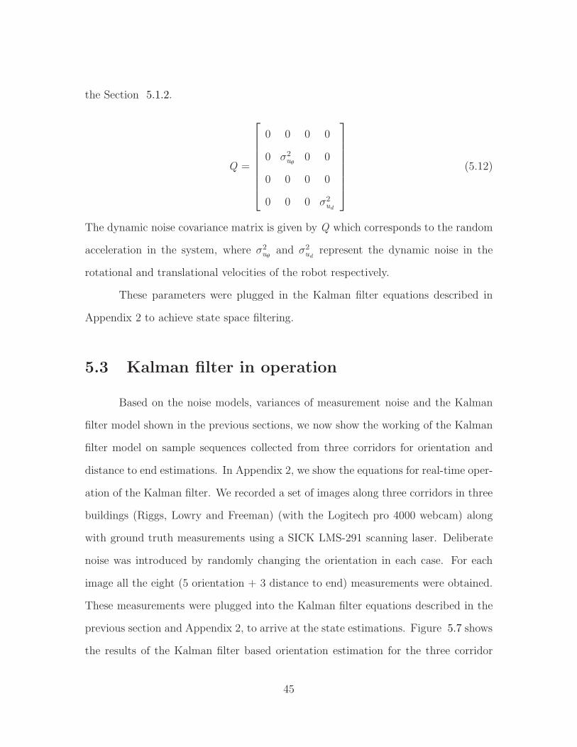
Figure 5.8: Distance to the end estimation for sequences of images collected in threecorridors. In each case, the unfiltered measurements (linear weighted average of thefive measurements),(blue solid) are shown along with the ground truth (red dashed)and the Kalman filtered estimate (green dotted).

49

Chapter 6

Corridor Junction Classification

6.1 Junction classification from monocular images

Apart from determining the orientation and distance to the end of the cor-

ridors for reactive navigation in unknown environments, we also show that image

entropy alone can be used to detect new corridors at a junction and to classify the

junction based on the information. The procedure followed for this experiment is as

follows. The robot was mounted with a SICK LMS-291 laser scanner, and a Logitech

QuickCam 4000 webcam and made to turn 360 at various types of indoor corridor

junctions (dead end (D), middle (M), L-junction (L), T-junction (T), cross-junction

(X)). Images were collected for junctions in 9 different corridors in 6 different build-

ings (Sirrine, Lowry, Freeman, Rhodes, Riggs and EIB). The robot was rotated at

a speed of 2 degrees per second, and data was stored at the rate of 0.5 Hz, leading

to densely sampled data approximately 1 degree apart. The laser provided depth

readings in a 180-degree horizontal plane in increments of 1 degree, leading to 180

laser depth readings per sample time. Only the reading corresponding to ) degrees

was considered for depth after smoothing. The image entropy is plotted along with

50

0 50 100 150 200 250 300 350 4000

0.5

1

1.5

2

2.5

3

3.5

4

4.5

5N

eare

st d

ista

nce

from

wal

l (10

−1 m

), E

ntro

py

theta (degrees)

EntropyDistance

0 50 100 150 200 250 300 350 4000

1

2

3

4

5

6

theta (degrees)

Nea

rest

dis

tanc

e fr

om w

all (

10−

1 m),

Ent

ropy

EntropyDistance

050 110 150 180 250 300 000 050 100 275 300 360

Figure 6.1: Top: Entropy (red solid line) and distance (blue dashed line) as the robotturned at a corridor T-junction in three different corridors. Distance was measuredusing a SICK scanning laser. Bottom: Images of the corridor approximately showingthe orientation with respect to the depth values corresponding to them above.

the actual depth readings from the laser scanner. See Figure 6.1.

For each 0 to 360 degree sequence, the entropy values are treated as a one-

dimensional vector. It is smoothed using a Gaussian filter and is convolved with the

derivative of a Gaussian. Boundaries are pruned and central zero-crossings are ob-

tained for peaks and valleys in the 1-D signal from the convolved derivative. Amongst

multiple close peaks/valleys detected, only the highest peak or lowest valley is chosen,

and the rest is discarded, thus enforcing a minimum threshold distance between two

peaks or valleys. In every signal, the number of peaks and the approximate angle

between them is extracted to arrive at the type of junction. The signal between two

valleys is taken and the mean (µ) and standard deviation (σ) are calculated. Gaus-

sians are fitted at each of the peaks using this information. The detected peaks and

fitted Gaussians for several corridors are shown in Figure 6.1.

51

0 50 100 1500

0.5

1

1.5

2

2.5

frame numberdist

ance

to n

eare

st w

all 1

0−1 m

, ent

ropy

entropydistance

0 50 100 150−0.5

0

0.5

1

1.5

2

2.5

frame numberdist

ance

to n

eare

st w

all 1

0−1 m

, ent

ropy

entropydistance

0 50 100 1500

0.5

1

1.5

2

frame numberdist

ance

to n

eare

st w

all 1

0−1 m

, ent

ropy

entropydistance

Freeman 1 Freeman 1 Freeman 1

0 50 100 1500

0.5

1

1.5

2

2.5

3

frame numberdist

ance

to n

eare

st w

all 1

0−1 m

, ent

ropy

entropydistance

0 50 100 1500

1

2

3

4

frame numberdist

ance

to n

eare

st w

all 1

0−1 m

, ent

ropy

entropydistance

0 50 100 1500

1

2

3

4

frame numberdist

ance

to n

eare

st w

all 1

0−1 m

, ent

ropy

entropydistance

Rhodes 2 Rhodes 3 Rhodes 3

0 50 100 150−1

0

1

2

3

frame numberdist

ance

to n

eare

st w

all 1

0−1 m

, ent

ropy

entropydistance

0 50 100 1500

0.5

1

1.5

2

2.5

frame numberdist

ance

to n

eare

st w

all 1

0−1 m

, ent

ropy

entropydistance

0 50 100 150−0.5

0

0.5

1

1.5

2

2.5

frame numberdist

ance

to n

eare

st w

all 1

0−1 m

, ent

ropy

entropydistance

Sirrine 1 Sirrine 1 Sirrine 1

0 50 100 1500

0.5

1

1.5

2

2.5

3

frame numberdist

ance

to n

eare

st w

all 1

0−1 m

, ent

ropy

entropydistance

0 50 100 150−0.5

0

0.5

1

1.5

2

2.5

frame numberdist

ance

to n

eare

st w

all 1

0−1 m

, ent

ropy

entropydistance

0 50 100 1500

0.5

1

1.5

2

2.5

3

frame numberdist

ance

to n

eare

st w

all 1

0−1 m

, ent

ropy

entropydistance


52

0 50 100 1500

1

2

3

4

frame numberdist

ance

to n

eare

st w

all 1

0−1 m

, ent

ropy

entropydistance

0 50 100 1500

0.5

1

1.5

2

frame numberdist

ance

to n

eare

st w

all 1

0−1 m

, ent

ropy

entropydistance

0 50 100 1500

0.5

1

1.5

2

2.5

frame numberdist

ance

to n

eare

st w

all 1

0−1 m

, ent

ropy

entropydistance

Freeman 1 Freeman 1 Freeman 1

0 50 100 1500

1

2

3

4

frame numberdist

ance

to n

eare

st w

all 1

0−1 m

, ent

ropy

entropydistance

0 50 100 1500

1

2

3

4

frame numberdist

ance

to n

eare

st w

all 1

0−1 m

, ent

ropy

entropydistance

0 50 100 1500

0.5

1

1.5

2

2.5

3

frame numberdist

ance

to n

eare

st w

all 1

0−1 m

, ent

ropy

entropydistance

Lowry 1 Lowry 1 Lowry 2

0 50 100 1500

1

2

3

4

frame numberdist

ance

to n

eare

st w

all 1

0−1 m

, ent

ropy

entropydistance

0 50 100 150−1

0

1

2

3

4

frame numberdist

ance

to n

eare

st w

all 1

0−1 m

, ent

ropy

entropydistance

0 50 100 1500

1

2

3

4

frame numberdist

ance

to n

eare

st w

all 1

0−1 m

, ent

ropy

entropydistance

Rhodes 2 Rhodes 3 Rhodes 3

0 50 100 1500

1

2

3

4

frame numberdist

ance

to n

eare

st w

all 1

0−1 m

, ent

ropy

entropydistance

0 50 100 1500

0.5

1

1.5

2

2.5

frame numberdist

ance

to n

eare

st w

all 1

0−1 m

, ent

ropy

entropydistance

0 50 100 150−1

0

1

2

3

4

frame numberdist

ance

to n

eare

st w

all 1

0−1 m

, ent

ropy

entropydistance


Figure 6.2: Corridor classification: Example junctions with Gaussian mixture modelsoverlaid on the entropy peaks. Entropy as seen is powerful in itself to determinecorridor depth when the depth change (due to structure) is significant. The greensquares and red circles correspond to the detected peaks and valleys, respectively.

53

6.2 Junction classification from omnidirectional im-

ages

Catadioptric sensors have an advantage over monocular cameras (even though

they are specialized) because they provide the robot with a 360 field of view thereby

giving more abundant and rich information, which can be exploited in different ways

for navigation [10]. The unwrapping of the image so obtained to a 1-D panaromic

stack is convenient for analysis. See some example corridor images in Figure 6.4.

Bonev et al. [10] have previously shown that entropy is powerful for determining

open corridors in omnidirectional images. We however have previously independently

shown that this works for standard monocular images in low-resolution. We show

some examples in Figure 6.2 that strengthens the hypothesis in [10]. We have also

shown in the previous section that the entropy peaks can be used to determine junc-

tion types in corridors. We show that the same technique can be applied to omnidirec-

tional images to determine corridor junction types based on entropy peaks detected.

Some examples are shown in Figure 6.5.

54

(a)

(b)

(c)

Figure 6.3: (a): Omnidirectional image of a corridor. The image was downsampledto 164×24 before processing(b):1-D panaromic rectified image. (c):The entropy mapof the 1-D panaromic stack of a sequence of images along the same corridor. Entropywas calculated for each column (10 pixel wide) in the gradient magnitude image.Dark tones correspond to low entropy and light tones correspond to high entropy.

55

Figure 6.4: Sample omnidirectional images obtained with a camera and a hyperbolicmirror (TOP) and the rectified panaromic images (BOTTOM).

56

0 200 400 600 800 10000

2

4

6

8

x (pixels)

Ent

ropy

(bi

ts/p

ixel

)

0 200 400 600 800 10000

2

4

6

8

x (pixels)

Ent

ropy

(bi

ts/p

ixel

)

Figure 6.5: The entropy peak detection method used for monocular images workswell on (unwrapped) omnidirectional images. The entropy values are smoothed usinga Gaussian filter and are convolved with the derivative of a Gaussian. Boundaries arepruned and central zero-crossings are obtained for peaks (red asterisk) and valleys inthe 1-D signal from the convolved derivative. Amongst multiple close peaks/valleysdetected, only the highest peak or lowest valley is chosen, and the rest are discarded,thus enforcing a minimum distance between two peaks or valleys. The signal betweentwo valleys is taken and the mean (µ) and standard deviation (σ) are calculated.Gaussians are fitted at each of the peaks using this information, shown as red solidcurves.

57

Chapter 7

Estimating Corridor Geometry for

Navigation

We present a minimalistic representation of the corridor geometry using low-

resolution images for autonomous mobile robot navigation. We show a combination of

percepts, orientation line and wall-floor boundary, to result in a three-line representa-

tion intersecting at the vanishing point. The orientation line can be used to keep the

robot oriented along the corridor and the wall-floor boundaries can be used to keep

the robot away from the walls (lateral limit). We also show that this representation

can be achieved consistently across different resolutions from 320 × 240 to 16 × 12

with very little loss of accuracy.

7.1 Minimalistic corridor geometry

7.1.1 Estimating the orientation line

The orientation line is estimated using three of the above describes methods

(maximum entropy, median of ceiling lights and maximum symmetry) for reasons

58

of simplicity. At standard resolution (320 × 240), the calculation of the median of

ceiling lights is corrupted by reflections. To solve this problem, we add an additional

constraint using local contrast [95] along with k-means to segment the bright pixels.

Only if local contrast exceeds a threshold, the pixels are considered to be from a light

source. See Appendix 3 for details. It can be seen from Figure 7.1 that the effect of

reflections are avoided to a great extent using this method. However, in low-resolution

images the effect of the method is negligible.

The maximum symmetry and maximum entropy based orientation estimations

however, remain the same. We combine the estimates as a weighted average: f (I ) =

αl(I )fl(I )+αh(I )fh(I )+αs(I )fs(I ). Because of the reliability of the bright pixels, we

set αl = 0.8, αh = αs = 0.1. An example result obtained for different resolutions is


7.1.2 Estimating the wall-floor boundary

We adapt the floor segmentation method introduced by Li and Birchfield [49]

which has been shown to be successfully robust to reflections on the floor. For the

seven different resolutions, we compute the minimum acceptance length of the hori-

zontal line segments lh as lh = ln ηd , where d =√w 2 + h2 is the length of the diagonal

of the image, w and h are the width and height of the image, respectively, and η = 5

is a scaling factor.

According to the floor segmentation method [49], there are three different

scores (structure score, homogeneous score, and bottom score) that contribute to the

final wall-floor boundary detection. When applying the method to different resolu-

tions, we notice the structure score always shows the best accuracy while the bottom

score always fails when decreasing the resolution. Therefore, we adapt the weights

59

Regular Ullman

Figure 7.1: Comparison between the median of ceiling lights obtained for high resolu-tion images using regular k-means and that by applying the local contrast threshold(described by Ullman [95]).

60

320x240 160x120 80x60 64x48

32x24 16x12 8x6

Figure 7.2: The orientation line estimate (vertical green line) for the images shown inFigure 1.1. Down to a resolution of 16×12, the results remain essentially unchanged.Only at the lowest resolution of 8×6 is the technique unable to recover the orientationline accurately.

for the three scores according to the resolution so that the Φtotal (ℓh) is relatively high

for line segments near the wall-floor boundary. At the same time, when combining

with the orientation line, we compute the intersection of the orientation line and the

wall-floor boundary, which is considered as the vanishing point. Then we apply the

line-fitting algorithm to both half wall-floor boundaries separated by the vanishing

point. Using the slopes and the computed vanishing point, it is easy to find the two

terminal points on the image border. Finally, we connect the vanishing point, two

terminal points, as well as the orientation line and obtain the structure of the corridor.

The sample results are shown in Figure 8.12 and the second row of Figure 7.4.

61

7.2 Minimalistic corridor reconstruction

7.2.1 Orientation line in the corridor

Estimating the pose of the robot or the orientation line of the robot in a

typical indoor corridor is one of the necessary tasks for robot exploration/navigation.

While many authors have contributed to this work, by estimating vanishing points

in a corridor, [80, 7, 58, 71], the emphasis is on clustering detected lines, which

perform poorly in low-resolution and textureless images because lines are not easily

detected in such images. A more recent approach by Kong et al. [43] approaches the

problem similarly but uses texture orientation rather than explicit line detection. In

their approach, Gabor filters yield texture estimates, and an adaptive voting scheme

allows pixels to decide the confidence of an orientation. However we show that not

only is our method better suited for indoor images in low-resolution, but is also much

faster. See Section 7.2.3.

7.2.2 Width of the corridor

The distance between the two end-points in the wall-floor boundary yields the

width of the corridor (in pixels). We use a homography obtained during a calibration

process to transform to world coordinates. The process is briefly illustrated in Figure

7.3. A square pattern on the floor and the corresponding real-world dimensions were

used to obtain a homography between the image plane and the top-down view of the

corridor. The homography was applied to the end points of the wall-floor boundary

to obtain the top-down view of the reconstructed corridor.

62

Figure 7.3: Top: A square with top-down ground truth world measurements (right)projects onto the image as a quadrilateral on the floor (left). The four points aresufficient for estimating a homography between the image and the top-down view ofthe corridor. Bottom: The homography is then applied to the end points of thewall-floor boundary to reconstruct the top-down view of the corridor. Shown on theright is a plot of such top-down coordinates (red dots) as the robot drives along astraight path (blue dashed line).

63

7.2.3 Lateral position in the corridor

The position of the orientation line with respect to the wall-floor boundaries

will give the lateral position in the corridor. The top down dimensions of the recon-

structed corridor gives us the distance from the center to the left wall and to the right

wall. This can be used to obtain the lateral position of the robot in the corridor. The

center of the corridor is assumed to be zero. For ground truth comparisons, the laser

span readings were converted from polar to Cartesian to give a top-down measure-

ment of the corridor at every instance of the image collection. Several examples are


64

320x240

160x120

80x60

64x48

32x24

16x12

8x6

Figure 7.4: Left: The wall-floor boundary found by the algorithm described in [49]for the different resolution images of Figure 1.1. The accuracy degrades slightly untilthe resolution of 32 × 24, after which the errors become more pronounced. Right:

The three-line model estimate of the corridor found by combining the orientation linewith the wall-floor boundary, on the same images.

65

Chapter 8

Experimental Results

To test the approaches shown for solving the first problem (estimating the

orientation and distance to the end), we analyze the accuracy of the various individual

measures for the orientation and distance to the end. Then we describe the combined

system and evaluate its performance exploring several unknown environments. For the

second problem (corridor classification) we show the classification results for different

buildings with different junction types. We also evaluate the classifier performance

for the parameters used. For the third problem (minimalistic corridor geometry),

we show orientation line estimated and wall-floor boundaries for different corridor

across different resolutions. We then show a combined system with the three-line

representation for all the resolutions. We evaluate the performance with respect to

ground truth measurements and show the error for each resolution tested on.

8.1 Orientation along the corridor

We collected data for 10 unique corridors in 5 different buildings on our cam-

pus, shown in Figure 8.1. Multiple corridors were used for the same building only

66

Figure 8.1: 10 distinct corridors in 5 different buildings. The inset shows the 32× 24downsampled version, upsampled to make it more visible. In lexicographic order,the corridors are Riggs-0, Riggs-1, Riggs-2, Riggs-3, Rhodes-4, Sirrine-0, Sirrine-2,Freeman-0, Lowry-0, Lowry-2, where the number indicates the floor.

when they were located on different floors and exhibited varying appearances. For

every corridor, at equally spaced 15 feet intervals along the corridor we rotated the

robot from −20 degrees to +20 degrees while collecting odometry data, laser readings,

and images. The equipment used was an ActivMedia P3AT mobile robot, a SICK

LMS-291 laser, and a forward-facing Logitech QuickCam Pro 4000 webcam. The

robot was rotated at a speed of 2 degrees per second, and data was stored at the rate

of 0.5 Hz, leading to densely sampled data approximately 1 degree apart. The laser

provided depth readings in a 180-degree horizontal plane in increments of 1 degree,

leading to 180 laser depth readings per sample time. The peak of these depth laser

readings, after smoothing, was used to estimate the ground truth orientation, except

for one corridor containing large specular surfaces (Lowry-0), where the heading was

obtained from the odometry readings.

Figure 8.2 shows the orientation estimates of the five different measures on six

example images from different corridors and buildings. For each image, the vertical

red line indicates the estimate of the corridor centerline. There is in general wide

agreement between the various measures, and their error with respect to ground

truth is generally less than about 5 degrees. Overall, the median of the bright pixels

67

yields the most accurate estimate, with the accuracy from entropy being only slightly

degraded. The other three techniques also produce good results, but their accuracy

is noticeably less. From the plots below, it can also be seen that the median of the

bright pixels yields a very sharp peak compared with the other measures.

To determine the broad applicability of the approach, Figure 8.3 shows the

results of the five measures on the database. Half of the data was used for developing

algorithm parameters, so these results are shown for the other half of the database.

The error bars show the range ±2σ capturing 95% of the data, where σ is the standard

deviation of the error. As can be seen, the error for entropy is generally less than 10

degrees, the error for bright pixels is less than 5 degrees, and the error for the other

techniques is less than approximately 15 degrees. For entropy and bright pixels, the

error does not vary significantly across headings, while for the other three measures

the error varies widely.

For driving a robot down the center of the corridor, the most important infor-

mation is whether the orientation estimate is in the correct direction. In other words,

the estimate should tell the robot to turn right when it is pointing to the left, and it

should tell the robot to turn left when it is pointing to the right. Figure 8.4 shows the

percentage of locations in which each of the five measures computes the correct sign

for the orientation, with the center of the image defined as the zero heading. Again,

outside a 5- to 10-degree range around the center of the corridor, both the entropy

and bright light measures nearly always produce the correct direction.

8.2 Distance to the end of the corridor

For the same 10 corridors mentioned earlier, we drove the robot down the

corridor three times: down the center of the corridor, down the left side (1.5 feet

68

0 10 20 30

6

6.1

6.2

6.3

6.4

6.5

image x axis (pixels)

entr

opy

(bits

per

pix

el)

0 10 20 305.2

5.4

5.6

5.8

6

6.2

6.4


entr

opy

(bits

per

pix

el)

0 10 20 30

5.2

5.4

5.6

5.8

6

6.2


entr

opy

(bits

per

pix

el)

0 10 20 30

5.4

5.6

5.8

6

6.2


entr

opy

(bits

per

pix

el)

0 10 20 305.2

5.4

5.6

5.8

6


entr

opy

(bits

per

pix

el)

0 10 20 30

5

5.5

6

6.5


entr

opy

(bits

per

pix

el)

0 10 20 30

4.4

4.6

4.8

5

5.2


Mut

ual I

nfor

mat

ion

(bits

per

pix

el)

0 10 20 303.5

4

4.5

5


Mut

ual I

nfor

mat

ion

(bits

per

pix

el)

0 10 20 30

3

3.5

4

4.5

5


Mut

ual I

nfor

mat

ion

(bits

per

pix

el)

0 10 20 30

3.5

4

4.5

5


Mut

ual I

nfor

mat

ion

(bits

per

pix

el)

0 10 20 30

3.8

4

4.2

4.4

4.6

4.8


Mut

ual I

nfor

mat

ion

(bits

per

pix

el)

0 10 20 30

3

3.5

4

4.5

5


Mut

ual I

nfor

mat

ion

(bits

per

pix

el)

0 10 20 300

0.5

1

1.5

2

2.5

3


Agg

rega

te P

hase

(ra

dian

s)

0 10 20 300

1

2

3

4

5

6


Agg

rega

te P

hase

(ra

dian

s)

0 10 20 300

1

2

3

4

5


Agg

rega

te P

hase

(ra

dian

s)

0 10 20 300

1

2

3

4

5


Agg

rega

te P

hase

(ra

dian

s)

0 10 20 300

1

2

3

4

5

6

7


Agg

rega

te P

hase

(ra

dian

s)

0 10 20 301

2

3

4

5

6

7


Agg

rega

te P

hase

(ra

dian

s)

0 10 20 300

5

10

15


brig

ht p

ixel

s

0 10 20 300

2

4

6

8

10

12

14


brig

ht p

ixel

s

0 10 20 300

2

4

6

8


brig

ht p

ixel

s

0 10 20 300

2

4

6

8


brig

ht p

ixel

s

0 10 20 300

2

4

6

8


brig

ht p

ixel

s

0 10 20 300

5

10

15


brig

ht p

ixel

s

Figure 8.2: Estimating the center of the corridor using various cues. Top rows:

Six example tiny corridor images, with the pixel column corresponding to the centerof the corridor overlaid for each of the five different methods: entropy, symmetry,aggregate phase, vanishing point, and bright pixels. Bottom rows: Plots of thefunction computed for four of these measures — No plot for vanishing point is shown,since the technique directly produces an estimate.

69

−20o −13.3o −6.7o 0o 6.7o 13.3o 20o

−20 −10 0 10 20−20

−15

−10

−5

0

5

10

15

20

ground truth angle (degrees)

estim

ated

ang

le (

degr

ees)

−20 −10 0 10 20−20

−15

−10

−5

0

5

10

15

20


estim

ated

ang

le (

degr

ees)

−20 −10 0 10 20−20

−15

−10

−5

0

5

10

15

20

ground truth angle (degrees)es

timat

ed a

ngle

(de

gree

s)

−20 −10 0 10 20−20

−15

−10

−5

0

5

10

15

20


estim

ated

ang

le (

degr

ees)

−20 −10 0 10 20−20

−15

−10

−5

0

5

10

15

20


estim

ated

ang

le (

degr

ees)

maximum entropy symmetry aggregate phase self-similarity bright pixels

Figure 8.3: Top: Sample images from the orientation experiment in one corridor.Bottom: Orientation estimate plots for the five measures on the database. Eachplot shows, for each angle of the robot, the mean estimated angle across the databasealong with error bars indicating indicates ±2σ, where σ is the standard deviation.The diagonal line is the ground truth. Note again the high accuracy of the brightpixels.

−20 −10 0 10 200

0.2

0.4

0.6

0.8

1

ground truth angle (degrees)perc

enta

ge o

f est

imat

ed a

ngle

s w

ith c

orre

ct s

ign

−20 −10 0 10 200

0.2

0.4

0.6

0.8

1


enta

ge o

f est

imat

ed a

ngle

s w

ith c

orre

ct s

ign

−20 −10 0 10 200

0.2

0.4

0.6

0.8

1


enta

ge o

f est

imat

ed a

ngle

s w

ith c

orre

ct s

ign

−20 −10 0 10 200

0.2

0.4

0.6

0.8

1


enta

ge o

f est

imat

ed a

ngle

s w

ith c

orre

ct s

ign

−20 −10 0 10 200

0.2

0.4

0.6

0.8

1


enta

ge o

f est

imat

ed a

ngle

s w

ith c

orre

ct s

ign

maximum entropy symmetry aggregate phase self-similarity bright pixels

Figure 8.4: Plots of the orientation sign estimates for the five techniques. Each plotshows, for each angle of the robot, the percentage of images across the database inwhich the technique estimated the sign of the orientation correctly, with the centerof the image corresponding to a heading of zero.

70

0 0.5 1 1.5 2 2.50

20

40

60

80

100

120

ground truth distance to end (m)

Tim

e−to

−co

llisi

on (

s)

0 0.5 1 1.5 2 2.50

10

20

30

40

50


Jeffr

ey D

iver

genc

e (b

its/p

ixel

)

0 0.5 1 1.5 2 2.50

0.2

0.4

0.6

0.8


Ent

ropy

(bi

ts/p

ixel

)

0 0.5 1 1.5 2 2.50

0.5

1

1.5

2

2.5


estim

ated

dis

tanc

e to

end

(m

)

0 0.5 1 1.5 2 2.5

0.5

1

1.5

2

2.5


estim

ated

dis

tanc

e to

end

(m

)

0 0.5 1 1.5 2 2.50

0.5

1

1.5

2

2.5


estim

ated

dis

tanc

e to

end

(m

)

time-to-collision Jeffrey divergence entropy

Figure 8.5: Top: The three measures plotted versus the distance from the robot tothe end of the corridor. As the robot approaches the end, the entropy and time-to-collision decrease, while the Jeffrey divergence increases. Each line is a separaterun of the robot along a different corridor / location within the corridor. Bottom:Estimated distance to the end of the corridor plotted against ground truth (obtainedfrom the laser) for all three measures. Each vertical error bar indicates ±2σ, whereσ is the standard deviation.

from the center), and down the right side (1.5 feet from the center). While driving,

the robot collected 640× 480 images along with their corresponding 180-degree laser

readings. The three measures for estimating the distance to the end were compared

with ground truth, which was estimated from the central laser reading after median

filtering.

Figure 8.5 shows the results of the three measures. After performing a linear fit

to determine the two scale factors α2 and α3, all three measures performed reasonably

well at estimating the distance to the end, with time-to-collision being the most

accurate. All measures performed more accurately as the robot approached the end

of the corridor, until a distance of about 0.25 meters.

71

8.3 Exploration in an unknown environment

The completed system consisted of the mobile base with a single forward-

facing camera on the front. The only input to the system consisted of the tiny

32× 24 downsampled grayscale images from the camera.

The exploration capability of the robot was tested in several corridors. The

robot did not have any knowledge of the corridor before the run, and its goal was to

autonomously explore the environment by repeatedly driving down the corridor and

turning at the end. The turning direction at the end of a corridor was determined by

attempting the two possibilities of turning right / turning left in an arbitrary order,

using the entropy to distinguish between an open side corridor and a wall. In the

event of a dead end, in which case both turning right and turning left are not possible,

the robot made a 180-degree turn to return along the direction from which it came.

Results of the system showing successful end-to-end autonomous exploration

in several different corridors are displayed in Figure 8.6. The robot was able to stay

in the center of the corridor, detect the end, stop, turn 90 degrees in the appropriate

direction, and continue driving. The layout of the buildings, along with the path

taken by the robot in each run, are shown in the figure. Note that the laser readings

were used only to generate the plots, not to guide the robot. We also conducted

experiments in which the robot started facing the wall, or started close to a wall; in

both cases the robot corrected its orientation and position and continued exploring the

environment. The longest successful exploration was a corridor in which the robot

continuously ran for 45 minutes, navigating a total (overlapping) distance greater

than 850 meters.

A few failure situations are also evident from the plots in the figure. In Riggs-0

and Lowry-0, the final corridor ends in a pair of transparent glass doors or reflective

72

0 10 20 30 40

−20

−15

−10

−5

0

5

10

x (m)

y (m

)1 2

34 5

0 10 20 30 40

0

10

20

30

x (m)

y (m

)

1

2 3

4

−30 −20 −10 0 10 20

0

10

20

30

x (m)

y (m

)

12

3

4 5

0 10 20 300

5

10

15

20

25

30

x (m)

y (m

)

1

2 3

wall which confuse all the methods for determining the end of the corridor. In Riggs-

1, the presence of a brightly textured vending machine in the final corridor causes

erroneous estimates for the robot orientation. Note that the robot successfully ex-

plores other corridors containing vending machines because the robot has sufficient

time to react, in this corridor the machine is located close to the turn so that it

dominates the robot’s field of view immediately after the final left turn. Images from

these environments are shown in Figure 8.7.

In the introduction, we referred to psychological evidence that humans do not

need to process image data continuously in order to successfully navigate an environ-

ment. And in fact, as a robot moves down a corridor, it is easy to see that consecutive

images usually differ from each other by only a small amount. Therefore, we compare

the entropy of consecutive images from the current frame t and previous frame t − 1,

73

−20 −10 0 10 20 300

10

20

30

40

x (m)

y (m

)

1

2

0 5 10 150

5

10

15

20

x (m)

y (m

)

1

3

5

2

4

−20 −10 0 10 20 30−10

0

10

20

30

40

50

x (m)

y (m

)

3

2

4

1

−25 −20 −15 −10 −5 0

0

5

10

15

20

25

y (m

)

1

2

4

3

0 10 20 30 40 50

0

10

20

30

x (m)

y (m

)

2 3

41

−20 0 20

0

10

20

30

x (m)

y (m

)

1

2 3

Figure 8.6: Exploration experiments for ten different corridors, showing is the pathtaken by the robot (red dashed, obtained from laser measurements) and the end-of-corridor detections (green asterisks) along different corridors (blue solid, manuallymeasured). The numbering shows the temporal sequence of the robot’s locationsfrom start to end. In lexicographic order, the corridors are Riggs-0, Riggs-1, Riggs-3,Lowry-0,Lowry-2, Freeman-0,Riggs-2, Sirrine-0, Sirrine-2 and Rhodes-4

74

(a) (b) (c) (d)

Figure 8.7: Problematic corridors: (a) reflective glass doors in Riggs-0, (b) reflectivewall in Lowry-0, and (c) soda machine in Riggs-1, and (d) glass structures and lackof ceiling lights in EIB-1.

normalized by the first frame of the corridor (which presumably is near the maxi-

mum, since the entropy difference decreases as the robot travels down the corridor):∣

∣H (V ; I (t))−H (V ; I (t−1))∣

∣ /H (V ; I (1)). A histogram of these normalized entropy

differences is shown in the top of Figure 8.8 for three different corridors, from which

it is clear that most differences are small. As a result, our final system processes each

image a minimal amount in order to determine whether the image needs to be fully

processed by the five methods for orientation and three methods for distance-to-the-

end. If the normalized entropy difference is less than 0.01 (10%), then no further

processing is performed on the image. The results of this rapid perception are shown

in the middle and bottom of the figure, from which it can be seen that nearly 80% of

the images are only minimally processed.

8.4 Computational efficiency

To perform the entire processing on a single image (all five measures for esti-

mating the orientation, plus all three measures for estimating the distance to the end),

the system takes 3.65 ms. However, the rapid perception module mentioned above

quickly determines whether the current image needs to be processed in its entirety.

This module requires just 0.28 ms to make that decision, and 80% of the images are

75

0 0.005 0.01 0.015 0.020

5

10

15

20

25

30

35

entropy difference between consecutive images

freq

uenc

y of

occ

uren

ce

0 0.005 0.01 0.015 0.020

5

10

15

20

25

30


freq

uenc

y of

occ

uren

ce

0 0.005 0.01 0.015 0.020

10

20

30

40

50


freq

uenc

y of

occ

uren

ce

0 500 1000 1500 2000 25000

20

40

temporal index

no. i

mag

es

0 500 1000 1500 2000 25000

20

40

temporal index

dist

ance

(m

)

0 500 1000 1500 2000 25000

20

40

temporal index

no. i

mag

es

0 500 1000 1500 2000 25000

20

40

temporal index

dist

ance

(m

)

0 500 1000 15000

20

40

temporal index

no. i

mag

es0 500 1000 1500

0

20

40

temporal indexdi

stan

ce (

m)

(a) Riggs-0 (b) Riggs-1 (c) Lowry-0

Figure 8.8: Rapid perception for three different corridors. Top: Histogram of nor-malized entropy difference between consecutive images; most values are less than 0.01.Middle: The number of images fully processed by the system versus the temporalindex in the image sequence; most images are discarded after the rapid perceptionprocessing. Each bin captures 50 consecutive images, so that complete processing ofall frames would be indicated by all bars reaching a height of 50. The percentageof frames fully processed, approximately 20%, is therefore the area under the curvedivided by the area of the rectangle of height 50 and length equal to the numberof frames in the sequence. Bottom: The distance from the robot to the end ofthe corridor versus the image index. By comparing the two plots for each corridor,note that when the robot nears the end of the corridor, the number of images fullyprocessed increases.

76

Image capture and display 0.04 msDownsampling 0.18 ms

Maximum Entropy 0.02 msMaximum Symmetry 0.16 msAggregate Phase 0.02 msVanishing point(self-similarity) 1.5 msMedian of bright pixels 1.39 ms

Time-to-collision 0.26 msEntropy 0.06 msJeffrey divergence 0.02 ms

Total 3.65 ms

Table 8.1: Performance: Time taken by the different vision modules.

not processed further. Therefore, the time needed to process an image frame, on av-

erage, is (0.8)(0.28)+ (0.2)(3.65) = 0.954 ms, which is equivalent to processing about

1000 frames per second. Stated another way, with a standard 30 Hz camera, the

system consumes only 3% of the CPU, thus freeing the processor for other concurrent

tasks that might be needed in a real system.

8.5 Corridor junction classification

The robot was mounted with a SICK LMS-291 laser scanner, and a Logitech

QuickCam 4000 webcam and made to turn 360 at various types of indoor corri-

dor junctions (dead end, middle, L-junction, T-junction, cross-junction). The image

entropy was plotted along with the actual depth readings from the laser scanner.

reading every 2 degrees. only used center reading of laser after median filtering.

(Sirrine, Lowry, Freeman, Rhodes).

The classification of the corridors using entropy peaks can be analyzed by

representing the results in a confusion matrix [42]. A confusion matrix is of size

m × m, where there are m labels and shows the percentage of predicted and actual

77

p n totalp’ True Positive False Positive P’n’ False Negative True Negative N’

Total p n

Table 8.2: Table representing the four outcomes of a problem. true positive, truenegative, false positive, false negative. These can be used to construct the ROC(receiver operating characteristics) curve.

classifications. Metrics accuracy, true positive rate, true negative rate, precision, false

positive rate, false negative rate can be calculated using the confusion matrix as shown

in Table 8.5. In signal detection theory, a receiver operating characteristic (ROC),

or simply ROC curve, is a graphical plot of the sensitivity, or true positive rate,

vs. false positive rate, for a binary classifier system as its discrimination threshold

is varied. The ROC can also be represented equivalently by plotting the fraction of

false negatives out of the positives (FAR = false acceptance rate) vs. the fraction

of true positives out of the negatives (TPR = true positive rate). Also known as a

Relative Operating Characteristic curve, because it is a comparison of two operating

characteristics (FAR and TPR) as the criterion changes.

TPR =FN

P=

TP

(TP + FN )(8.1)

FAR =FP

N=

FP

(FP + TN )(8.2)

There are two discriminating criteria in the algorithm used for detecting/clas-

sifying peaks. One is the Gaussian kernel size used for smoothing k (σ is dependent

on k by the following relationship σ =√

k/2. The second parameter is the minimum

distance between peaks w . By keeping the k as 80 by trial and error, we plot the ROC

curve for varying w to obtain the optimum value. The ERR (Equal error rate) is the

78

D M L T XD 3 3 0 1 0M 0 30 0 1 0L 0 1 3 4 0T 0 2 0 5 0X 0 0 0 0 1

Table 8.3: Corridor classification

0 0.2 0.4 0.6 0.8 10

0.2

0.4

0.6

0.8

1

FAR (false acceptance rate)

TR

P (

true

pos

itive

rat

e)

Figure 8.9: ROC curve depicting the success of the classifier. The ERR was found tobe 0.14 and the corresponding value of the parameter w was found to be 32.

endtabular

value at which the FAR = (1-TPR) and we can identify the corresponding values of

the parameter for that. Its corresponds to the best performance that can be obtained

from the classifier. See Figure 8.9.

8.6 Minimalistic corridor representation and re-

construction

For orientation, we collected data for 4 different buildings, 8 unique corridors

(1 training + 7 for testing). For every unique corridor, at equally spaced intervals

79

along the corridor (15 ft), we rotated the robot from −20to + 20 and collected

corresponding odometry (heading), laser readings (span of −90to+90) and images.

We ran the entropy detector, light detector and symmetry detector on the images

and compared with ground truth (odometry and/or laser). Since a linear relationship

exits between the detected pixel location corresponding to the center of the corridor

and the robot orientation as explained in previous sections, we use either the estimate

fl or (fh + fs)/2.

For wall-floor boundary and corridor reconstruction, we collected data for 11

distinct corridors in 6 different buildings. Drove robot three times (middle, left, right

separated by 1.5 feet) along each corridor. and collected images along with their

corresponding laser readings (−90to + 90 sweep)

The parameters for a linear fit between the location of the orientation line

and predicted orientation were estimated by using one of the corridors as a training

set. Using the trained parameters, the orientations for all the other data for the

remaining 7 test corridors (θ) were predicted from the mean pixel locations using the

above equations. The mean error between ground truth (laser) and predicted values

of heading was calculated for each of the 7 resolutions considered 320×240, 160×120,

80× 60, 64× 48, 32× 24, 16× 12 and 8× 6. The results are shown in Figure 8.10.

We show that, with indoor low-resolution images the results of Kong et al.

[43] are significantly less accurate for determining the wall-floor boundary as well as

the orientation line (and therefore the vanishing point). See Figure 8.11 for some

examples.

A comparison of our results on four different resolutions is shown in Figure

8.15. It can be seen that the results are consistent across all the four resolutions,

320 × 240, 80× 60, 32 × 24 and 16× 12. This strengthens our argument in favor of

using low-resolution information for basic navigation tasks.

80

320x240 160x120 80x60 64x48 32x24 16x12 8x60

1

2

3

4

5

6

image resolution

mea

n er

ror

(deg

rees

)

corr−1corr−2corr−3corr−4corr−5corr−6corr−7

320x240 160x120 80x60 64x48 32x24 16x12 8x61

1.1

1.2

1.3

1.4

1.5

1.6

1.7

1.8

1.9

image resolution

mea

n er

ror

(deg

rees

)

Figure 8.10: Minimalistic geometric information is obtained by the algorithm at verylow image resolutions. Top: Mean error (degrees) for each of the 7 test corridors.Bottom: Mean error (degrees) of all the 7 test corridors. The orientation estimationerror remains relatively stable across different image resolutions. In fact the errordrops for a few corridors at 32 × 24, primarily due to the fact that downsamplingremoves artifacts such as reflections and other noise on the walls and floor.

81

320x240 80x60 32x24

320x240 80x60 32x24

Figure 8.11: Comparison between our results (three yellow lines) and those of Konget al. [43] (pink region). Our algorithm achieves more accurate estimation of boththe orientation line and the wall-floor boundary in indoor scenes, particularly at lowresolutions.

82

320x240 80x60 32x24

Figure 8.12: Additional results for other corridors, including one without ceilinglights. In some cases, the low-resolution images yield more accurate results.

83

GT

−2 −1.5 −1 −0.5 0 0.5 1 1.5 20

5

10

15

20

25

x (m)

y (m

)

−2 −1.5 −1 −0.5 0 0.5 1 1.5 20

5

10

15

20

25

x (m)

y (m

)

−2 −1.5 −1 −0.5 0 0.5 1 1.5 20

5

10

15

20

25

x (m)

y (m

)

320x240

−2 0 20

5

10

15

20

25

x (m)

y (m

)

−2 0 20

5

10

15

20

25

x (m)

y (m

)

−2 0 20

5

10

15

20

25

x (m)

y (m

)

160x120

−2 0 20

5

10

15

20

25

x (m)

y (m

)

−2 0 20

5

10

15

20

25

x (m)

y (m

)

−2 0 20

5

10

15

20

25

x (m)

y (m

)

80x60

−2 0 20

5

10

15

20

25

x (m)

y (m

)

−2 0 20

5

10

15

20

25

x (m)

y (m

)

−2 0 20

5

10

15

20

25

x (m)

y (m

)

64x48

−2 0 20

5

10

15

20

25

x (m)

y (m

)

−2 0 20

5

10

15

20

25

x (m)

y (m

)

−2 0 20

5

10

15

20

25

x (m)

y (m

)

84

32x24

−2 0 20

5

10

15

20

25

x (m)

y (m

)

−2 0 20

5

10

15

20

25

x (m)

y (m

)

−2 0 20

5

10

15

20

25

x (m)

y (m

)

16x12

−2 0 20

5

10

15

20

25

x (m)

y (m

)

−2 0 20

5

10

15

20

25

x (m)

y (m

)

−2 0 20

5

10

15

20

25

x (m)

y (m

)

8x6

−2 0 20

5

10

15

20

25

x (m)

y (m

)

−2 0 20

5

10

15

20

25

x (m)

y (m

)

−2 0 20

5

10

15

20

25

x (m)

y (m

)

Left Center Right

Figure 8.13: Corridor structure reconstruction from the wall-floor boundary, displayedas a top-down view. The topmost row in blue shows the ground truth location ofthe walls (Cartesian conversion of polar laser readings), and the next 7 rows in redshow the reconstruction results from the wall-floor boundaries on different resolutionimages. Each column represents a different run of the robot in the same corridor,with the robot placed at a different lateral position in the corridor for each run (Theposition of the robot is shown by the dotted line at 0). Surprisingly, the structurewas captured accurately in all resolutions. The error in the results for 86 resolutionfor the central trial run are spikes that become more pronounced when warped usingthe floor-image homography.

85

320x240 160x120 80x60 64x48 32x24 16x12 8x60

0.05

0.1

0.15

0.2

0.25

image resolution

mea

n er

ror

(m)

leftcenterright

320x240 160x120 80x60 64x48 32x24 16x12 8x60

0.05

0.1

0.15

0.2

0.25

0.3

0.35

0.4

image resolution

mea

n er

ror

(m)

leftcenterright

Figure 8.14: Top: Mean error (m) for estimating the lateral position of the robotfor three runs in a single corridor. The structure was accurately captured in all threecases. Bottom: Mean error (m) for the estimation of the corridor width. There isnot much difference in estimation error rates across the different resolutions, and infact the error drops in some cases for 32x24 and 16x12 sizes due to the removal ofnoise and artifacts by downsampling.

86

Frame 002 Frame 053 Frame 102



Figure 8.15: Showing four different resolutions (320 × 240, 80 × 60, 32 × 24 and16 × 12), with minimalistic geometry estimation for corridor sequences. It can beseen that the results show consistent success across varying resolutions and in comecases better results for the lower resolutions.

87

Chapter 9

Conclusion

The study of low-resolution images plays an important role in the understand-

ing of visual scenes. Interpretation of scenes for primitive tasks can be accomplished

using information obtained from images at exceedingly low-resolutions represented by

less than 5000 bits at every frame captured. The ability to understand the elementary

properties of an image at lower resolutions may be the key to solving a large number

of computer vision tasks at increasingly higher orders of speed. Some standard chal-

lenges faced by standard computer vision algorithms such as lack of texture and lack

of edges are addressed well by low-resolution techniques. Optimization of speed is

also achieved as a result of using low-resolution images that is conducive for systems

like hand-held devices and micro-embedded devices which are constrained in memory

and processor speed due to miniaturization. Furthermore there is evidence to show

that certain processes (peripheral vision) occur in low-resolution in humans motivat-

ing the need for developing algorithms in computer vision that can successfully work

with low-resolution images.

88

9.1 Contributions

This work represents a collection of some algorithms that work on exceedingly

low-resolution images to provide basic information for indoor robot navigation. The

main contributions of this dissertation are listed below:

9.1.1 Autonomous exploration

We have presented a low-resolution vision-based robot exploration system that

can navigate down the center of a typical unknown indoor corridor, and turn at the

end of the corridor. The exploratory behavior of a mobile robot is modeled by a set of

visual percepts that work in conjunction to correct its path in an indoor environment

based on different measures. Special emphasis is placed on using low-resolution images

for computational efficiency, and on measures that capture information content that

cannot be represented using traditional point features and methods. The resultant

algorithm enables end-to-end navigation in indoor environments with self-directed

decision making at corridor ends, without the use of any prior information or map.

The primary contribution of this work is the spatio-temporal compression of image

information that is needed for computing navigation parameters of the robot, yielding

a high computational efficiency while maintaining robustness.

We throw away 99.75% of spatial information (downsampling) and 80% of

temporal information (rapid perception), leading to an algorithm that works on just

0.02% of the information available. The advantage of such information reduction

is not only the tremendous computational efficiency which frees processor cycles to

perform higher-level tasks such as recognition, but also the proof-of-concept regarding

the amount of information needed for a particular task, in the spirit of minimalistic

sensing.

89

9.1.2 Junction classification

We have presented a classification of junction types for indoor environments

using information theory. Our approach showed a correlation between image entropy

and corridor depth. We show a classifier that it built using entropy values mea-

sured as a robot turns at corridor junctions that classifies five different junction types

(dead-end, middle, T-junction, L-junction, X-junction) with reasonable accuracy. We

extend the concept to unwrapped omnidirectional images and we show that the same

algorithm can be used to detect and classify corridors in such images with the added

advantage that only a single image is needed at each junction for such a classifica-

tion. The proposed algorithm was tested on images from several corridors showing

the feasibility of using entropy for detecting open corridors.

9.1.3 Minimalistic corridor representation

We have proposed an algorithm to extract a minimalistic geometric representa-

tion of a typical indoor corridor environment using low resolution images. Motivated

by the “selective degradation hypothesis,” our approach exploits the redundancy of

image information in order to extract useful information for mobile robotic tasks

with minimal processing. Our algorithm combines two ideas: extracting the wall-

floor boundary by combining intensity edges and specular reflection removal, and

centerline estimation using a combination of information theoretic cues and bright

pixel estimation. Previous approaches for these problems have been extended and

modified to facilitate low resolution processing.

The proposed algorithm was tested on images from several different corridors,

showing that the accuracy of the estimation of the orientation line or corridor geom-

etry changed very little even when more than 99% of the original information was

90

discarded by downsampling the image to an extremely low resolution. Our approach

can be seen as an exploration into identifying how much information is needed for

basic mobile robot tasks such as corridor exploration and navigation. By reducing

the resolution required for these basic tasks, the CPU time is freed for other tasks

that potentially require higher resolutions and more involved processing.

9.2 Future work

One of the major outcomes of our research endeavor is the presentation of a set

of techniques using information theory to identify the optimal resolution needed for

robot exploration. The same technique can be used to develop a general methodology

for several such applications and new problems in computer vision. Information

theory can be used to determine the amount of information needed to perform a

specific tasks. Some examples include determining the resolution for automatic target

recognition (ATR) and the resolution needed for video transmission.

There is much room for improvement in this line of work. First, all the al-

gorithms are challenged by specular or transparent surfaces, particularly when they

dominate the field of view. However, this limitation does not seem to be intrinsic to

the reduced amount of information, since a human viewer has no trouble interpret-

ing the low-resolution information. This leads to the question of exploring atypical

corridors and environments in which the algorithm currently fails. A potential task

could be to tailor the information theoretic measures combined with other measures

to achieve autonomous exploration in different indoor structures like atriums, court-

yards, lounges, office spaces, labs, and rooms in general, where the general structure

of the corridor could change from being long and rectangular to a square room, curved

structures, corridors, and so on. Apart from exploration such indoor environments

91

would also require some sort of dynamic obstacle avoidance. One suggestion would

be the use of relative entropy and crude optical flow techniques to detect and avoid

obstacles.

Another improvement would be to combine the low-level exploration capabili-

ties of such a robot with high-level recognition algorithms to provide a more detailed

sense of the robot’s location within the environment by recognizing landmarks. Ul-

timately, we believe that minimalistic low-resolution sensing is a promising approach

for low-level mobile robot tasks such as navigation and exploration.

We intend to explore the concept of self-similarity for vanishing points over

different scales and study the effect of scale both spatially and temporally for robot ex-

ploration tasks. Experiments performed with even lower spatial resolutions of 16×12

and 8 × 6 will help establish the spatial limit for different measures. Other future

work may involve achieving localization by combining this exploration technique with

existing vision based SLAM algorithms. The ultimate goal is to achieve local-global

localization by an autonomous navigating robot in an environment-independent man-

ner with strong emphasis on low-resolution and simplicity of the algorithms used.

92

Appendices

93

Appendix A

Time-to-contact Relative to a

Planar Surface

Horn et al. [29] have described the calculation of time-to-contact using spatial

and temporal image derivatives and can be computed using just two frames in a se-

quence. The system does not use any tracking or calibration. The camera is assumed

to be moving perpendicular to a planar surface.

If the distance from the approaching surface is Z , then the time-to-contact is

defined as

T =−ZdZdt

where dZdt

is the derivative of the distance with respect to time. According to perspec-

tive projection equations, if S is the length of the cross-section of the approaching

planar object and s is the size of its image, then, sf= S

Zwhere f is the focal length

of the camera, which implies that S dZdt

+ Z dsdt

= 0 (see Figure A.1).

94

Figure A.1: Perspective projection.

Then S dZdt

= −Z dsdt

which implies that

−ZdZdt

= τTTC =Sdsdt

(A.1)

Considering the brightness constancy assumption of an image E , (the bright-

ness of a pixel corresponding to a point on the object does not change with time), we

have

E (x +∆x , y +∆y , t +∆t) = E (x , y , t)

Assuming small motion between successive frames (small ∆x and ∆y), the above can

be expanded using first order Taylor’s series to get

Ex

dx

dt+ Ey

dy

dt+ Et = 0

or

uEx + vEy + Et = 0 (A.2)

where u = dxdt

and v = dy

dtrespectively , Ex = ∂E

∂xand Ey = ∂E

∂yare spatial image

95

brightness derivatives and Et =∂E∂t

is the temporal brightness derivative.

Once again obtaining perspective projection equations of the camera

x

f=

X

Zand

y

f=

Y

Z(A.3)

where X , Y , and Z are coordinates of a point in space and x , y are corresponding

image coordinates. Differentiating equation (A.3) with respect to time, we get

u

f=

U

Z− X

Z

W

Zand

v

f=

V

Z− Y

Z

V

Z(A.4)

where U , V , W are temporal derivatives of X , Y , Z respectively and represent

velocity of the point on the object relative to the camera. u, v are temporal derivatives

of x and y (the motion field in the image). Substituting equation (A.3) in equation

(A.4), we get

u

f=

U

Z− x

f

W

Z, and

v

f=

V

Z− y

f

V

Z(A.5)

which leads to

u =1

Z(fU − xW ) and v =

1

Z(fV − yW ) (A.6)

Considering the simple case where the translation is perpendicular to the op-

tical axis (see Figure A.2), U and V can be set to 0 in equation (A.6).

u = −xW

Zand v = −y

V

Z(A.7)

96

Figure A.2: Camera moving such that optical axis is perpendicular to the approachingsurface.

Substituting equation (A.7) in equation (A.2), we get

− W

Z(xEx + yEy) + Et = 0 (A.8)

or

CG + Et = 0 (A.9)

where C = −WZ

from equation (A.1) and is the inverse of TTC, and G = xEx + yEy .

Formulating a least squares method to minimize∑

(CG + Et)2 where the sum

is over all pixels of interest, which could be the whole image, we get

∑

(CG + Et)G = 0

C =

∑

G (x , y)Et

−∑

(G (x , y))2(A.10)

It is evident that when C increases, TTC decreases. Intuitively this explains

that as the camera approaches the surface being viewed, the temporal change in

brightness values increases rapidly and the spatial change decreases (because when

97

the object/surface grows bigger, the sum of spatial gradients is lower), and therefore

the TTC decreases as the object/surface looms closer to the camera.

98

Appendix B

Kalman Filter

If we consider a process of a system described by a linear model, in discrete

time, we can describe the process state, the input, the measurements and the measure-

ment and process noise. The Kalman filter is a powerful state estimation technique

that can then be used to estimate the state (unknown) of the system by using a

sequence of measurements and the input. The Kalman filter can produce true values

of measurements by predicting a state value, while estimating the uncertainty of the

predicted value, and computing a weighted average of the predicted value and the

measured value where the weights are associated with the noise covariances in the

measurements and the process [28]. For the success of a Kalman filter there are two

important assumptions. One is that the process has a linear model. The other is that

the noise (measurement and process) have a normal distribution. According to the

descriptions of Bishop and Welch [99], the equations of the Kalman filter fall into two

groups: time update equations and measurement update equations. The time update

equations are responsible for incorporating a new measurement into the a priori esti-

mate to obtain an improved a posteriori estimate. The time update equations can be

described as predictor equations, and the measurement update equations as corrector

99

equations.

B.1 Kalman filter, matrix notation

This section is described from class notes [28]. We show here for illustration,

a two variable state (position and velocity). We will now proceed to show the setting

up of the Kalman filter essentials in matrix form that will make is easier to set up

the equations. The measurements can be represented as follows (we assume a linear

relationship between the state and the measurements).

Yt = MXt + Nt (B.1)

where Yt is the measurements, Xt is the actual state of system(position and velocity)

at time t , M is the observation matrix (the part of system that is observable and

this constitutes measurements from different sensing modalities in general) and Nt

Random noise during sensing. In this illustration, only the position was measured at

each instance of time.

[ yt ] = [ 1 0 ]

xt

xt

+ [ nt ] (B.2)

Similarly, the state transition can be written as

Xt+1 = ΦXt + Ut (B.3)

where Ut represents the random dynamics between t and t +1, Xt+1 the actual state

of system at time t + 1 and Φ is the state transition matrix. We are assuming a

100

constant velocity model here. The detailed equation is re-written as

xt+1

˙xt+1

=

1 T

0 1

xt

xt

+

0

ut

(B.4)

where ut is the random acceleration during t ...t+1. For simplicity, the dynamic noise

during T , is assumed to be zero. This leads us to,

Xt+1 = ΦXt (B.5)

The filtering equation can be written as

Xt ,t = Xt ,t−1 +Kt(Yt −MXt ,t−1) (B.6)

where Xt ,t−1 is the predicted state from previous measurements, Xt ,t is the Kalman

filtered state from two estimates, Kt is the Kalman gain matrix (weighting of esti-

mates). The Kalman gain is calculated at every time step as follows

Kt = St ,t−1 +M T[

Rt +MSt ,t−tMT]−1

(B.7)

where St ,t−1 is the predicted covariance from previous estimates and Rt observation

noise covariance. An estimate of our accuracy at prediction is also calculated at each

step. The prediction can be written as

St+1,t = ΦSt ,tΦT +Qt (B.8)

101

where Qt dynamic noise covariance. The update of the covariance can be written as:

St ,t = [I − KtM ]St ,t−1 (B.9)

where I identity matrix.

B.2 Kalman filter in operation

The Kalman filter algorithm works in a loop with predict/update calculations

at eat time-step. We start by assuming in most cases that the state is unknown. In

this illustration, we assume zero position and velocity. The initial prediction is also

assumed to be zero (or unknown).

X0,0 = 0X1,0 = 0 (B.10)

The measurement noise covariance matrix is known. The measurement noise

can be obtained in various ways by observing the measurements for a specific position

over a period of time. Assuming a constant velocity model, we have

R = [σ2] (B.11)

The dynamic noise covariance matrix is

Q =

0 0

0 σ2u

(B.12)

where σu is the dynamic state noise and described the random acceleration in the

system. This is in general very difficult to measure and is obtained by tuning the

102

Kalman filter once the other constants are established.

We initialize S , the accuracy of the predictions to the dynamic covariance Q for

simplicity.

S0,0 = S1,0 = Q (B.13)

The following steps are repeated in a loop for Kalman filter operation and at

the end of each loop t is incremented.

Kt = St ,t−1MT [MSt ,t−1M

T + R]−1 (B.14)

Xt ,t = Xt ,t−1 +Kt [Yt −MXt ,t−1] (B.15)

St ,t = [I − KtM ]St ,t−1 (B.16)

Xt+1,t = ΦXt ,tSt+1,1 = ΦXt ,tSt ,tΦT +Qt (B.17)

103

Appendix C

Visual Detection of Light Sources

In a classic paper Ullman [95] describes six factors that are associated with

the detection of light sources in an image and therefore can be used to differentiate it

from the specular reflections. This is of enormous importance in indoor environments

where reflections occur far too often.

• The highest intensity in the visual field: Ullman states that having the highest

intensity in the scene is neither a necessary nor a sufficient condition for a light

source. Reflections and light sources often have the same intensities.

• High absolute intensity value: Pixels associated with a light source need not

have high absolute intensity. There are examples of dim lamps viewed against

a dark background as an example.

• Local contrast: Local contrast is an important and differentiating factor to

be considered for evaluating a point as a light source. The contrast between

intensity I1 and intensity I2 can be defined as I1−I2I1+I2

, according to Ullman. This

happens to be a monotonic function of I1I2

indicating how many timed a pixel is

brighter than another (neighboring pixel).

104

• Global contrast: Contrast when applied globally in the image compares the

brightest and the darkest intensities in the image.

• Intensity compared with the average intensity in the scene: Another factor that

has been considered is the influence of changes in average illumination. It was

deemed by Ullman that it does not affect the detection rate of light sources.

• Lightness computation: Lightness can be used to differentiate between sharp

intensity changes and the gradual intensity changes. In other words intensity

gradient along a certain direction can be used to determine the presence of a

light source. Sharp intensity changes signify the presence of a light source.

It can be seen from the discussion of the factors that the only two factors

which play a role in determining the light sources are ‘contrast’ and ‘lightness’.

105

Bibliography

[1] N. Ancona and T. Poggio. Optical flow from 1-D correlation: Application toa simple time-to-crash detector. International Journal of Computer Vision,14(2):131–146, Mar. 1995.

[2] J. Andre, D. A. Owens, and L. O. Harvey, Jr., editors. Visual perception :The influence of H. W. Leibowitz. Washington, DC: American PsychologicalAssociation, 2003.

[3] M. Atallah. On symmetry detection. In IEEE Transactions on Computers,34(‘7):663–666, 1985.

[4] A. Basu and X. Li. A framework for variable-resolution vision. In Proceedingsof the International Conference on Computing and Information: Advances inComputing and Information, pages 721–732, 1991.

[5] H. Bay, A. Ess, T. Tuytelaars, and L. V. Gool. SURF: Speeded up robustfeatures. Computer Vision and Image Understanding, 110(3):346–359, June2008.

[6] H. Bay, T. Tuytelaars, and L. V. Gool. SURF: Speeded up robust features. In9th European Conference on Computer Vision, Graz Austria, May 2006.

[7] E. Bayramoglu, N. Andersen, N. Kjolstad Poulsen, J. Andersen, and O. Ravn.Mobile robot navigation in a corridor using visual odometry. In InternationalConference on Advanced Robotics, pages 1 –6, June 2009.

[8] G. Blanc, Y. Mezouar, and P. Martinet. Indoor navigation of a wheeled mobilerobot along visual routes. In Proceedings of the IEEE International Conferenceon Robotics and Automation (ICRA), pages 3354–3359, 2005.

[9] J.-L. Blanco, J.-A. Fernandez-Madrigal, and J. Gonzalez. A new approachfor large-scale localization and mapping: Hybrid metric-topological SLAM. InProceedings of the International Conference on Robotics and Automation, 2007.

[10] B. Bonev, M. Cazorla, and F. Escolano. Robot navigation behaviors basedon omnidirectional vision and information theory. Journal of Physical Agents,1(1):27–35, September 2007.

106

[11] J. C. Brooks and D. A. Owens. Effects of luminance, blur, and tunnel visionon postural stability. Journal of Vision, 1(3):304, 2001.

[12] J. M. Buhmann, W. Burgard, A. B. Cremers, D. Fox, T. Hofmann, F. E.Schneider, J. Strikos, and S. Thrun. The mobile robot RHINO. AI Magazine,16(2):31–38, 1995.

[13] Z. Chen and S. T. Birchfield. Qualitative vision-based mobile robot naviga-tion. In Proceedings of the IEEE International Conference on Robotics andAutomation (ICRA), pages 2686–2692, May 2006.

[14] M. Cho and K. Lee. Bilateral symmetry detection via symmetry-growing. InIn the Proceedings of the British Machine Vision Conference, pages 1–8, 2009.

[15] K. Choi, S. Bae, Y. Lee, and C. Park. A lateral position and orientation esti-mating algorithm for the navigation of the vision-based wheeled mobile robotin a corridor. In SICE 2003 Annual Conference, volume 3, 2003.

[16] Y.-H. Choi, T.-K. Lee, and S.-Y. Oh. A line feature based SLAM with low graderange sensors using geometric constraints and active exploration for mobilerobot. Autonomous Robots, 24(1):13–27, January 2008.

[17] D. Coombs, M. Herman, T. Hong, and M. Nashman. Real-time obstacle avoid-ance using central flow divergence and peripheral flow. IEEE Transactions onRobotics and Automation, 14(1):49–59, Feb 1998.

[18] A. J. Davison and N. Kita. 3D simultaneous localisation and map-buildingusing active vision for a robot moving on undulating terrain. In Proceedingsof the IEEE Conference on Computer Vision and Pattern Recognition, pages384–391, 2001.

[19] A. J. Davison and N. Kita. Sequential localization and map-building forreal-time computer vision and robotics. Robotics and Autonomous Systems,36(4):171–183, 2001.

[20] A. J. Davison and D. W. Murray. Simultaneous localization and map-buildingusing active vision. IEEE Transactions on Pattern Analysis and Machine In-telligence, 24(7):865–880, July 2002.

[21] A. J. Davison, I. D. Reid, N. D. Molton, and O. Stasse. MonoSLAM: Real-time single camera slam. IEEE Transactions on Pattern Analysis and MachineIntelligence, 29(6):1052–1067, June 2007.

[22] G. N. DeSouza and A. C. Kak. Vision for mobile robot navigation: A survey.IEEE Transactions on Pattern Analysis and Machine Intelligence, 24(2):237–267, 2002.

107

[23] F. Escolano, B. Bonev, P. Suau, W. Aguilar, Y. Frauel, J. Saez, and M. Ca-zorla. Contextual visual localization: cascaded submap classification, optimizedsaliency detection, and fast view matching. In IEEE International Conferenceon Intelligent Robots and Systems, 2007.

[24] S. Han, G. W. Humphreys, and L. Chen. Uniform connectedness and clas-sical gestalt principles of perceptual grouping. Perception & Psychophysics,61(4):661–674, 1999.

[25] C. G. Harris and M. Stephens. A combined corner and edge detector. InProceedings of the 4th Alvey Vision Conference, pages 147–151, 1988.

[26] S. Hayashi and O. Hasegawa. Detecting faces from low-resolution images. InProceedings of the 7th Asian Conference on Computer Vision, pages 787–796,2006.

[27] H. Hirschmuller. Stereo processing by semi-global matching and mutual in-formation. IEEE Transactions on Pattern Analysis and Machine Intelligence,30(2):328–341, Feb. 2008.

[28] A. Hoover, 2006. Class Notes in Analysis of Robotic Systems.

[29] B. K. P. Horn, Y. Fang, and I. Masaki. Time to contact relative to a planarsurface. IEEE Intelligent Vehicles Symposium, pages 68–74, June 2007.

[30] I. Horswill. Specialization of perceptual processes. Technical Report AITR-1511, MIT-AI, 1994.

[31] I. D. Horswill. Polly: A vision-based artificial agent. In Proceedings of theNational Conference on Artificial Intelligence, pages 824–829, 1993.

[32] G. M. Jenkins and D. G. Watts. Spectral Analysis and its applications. Holden-Day, 1968.

[33] S. D. Jones, C. S. Andersen, and J. L. Crowley. Appearance based processes forvisual navigation. In Proceedings of the IEEE/RSJ International Conferenceon Intelligent Robots and Systems (IROS), pages 551–557, 1997.

[34] T. Judd, F. Durand, and A. Torralba. Fixations on low-resolution images.Journal of Vision, 11(4):1–20, 2011.

[35] A. A. Kalia, G. E. Legge, and N. A. Giudice. Learning building layouts withnon-geometric visual information: The effects of visual impairment and ages.Perception, 37(11):1677–1699, Nov 2008.

[36] K. Kanatani. Symmetry as a continuous feature. IEEE Transactions on PatternAnalysis and Machine Intelligence, 19(3):246–247, Mar. 1997.

108

[37] N. Karlsson, E. D. Bernard, J. Ostrowski, L. Goncalves, P. Pirjanian, andM. E. Munich. The vSLAM algorithm for robust localization and mapping. InProceedings of the IEEE International Conference on Robotics and Automation(ICRA), pages 24–29, 2005.

[38] J. Kim, V. Kolmogorov, and R. Zabih. Visual correspondence using energyminimization and mutual information. In Proceedings of the International Con-ference on Computer Vision, 2003.

[39] J. Klippenstein and H. Zhang. Quantitative evaluation of feature extractorsfor visual SLAM. In CRV ’07: Proceedings of the Fourth Canadian Conferenceon Computer and Robot Vision, pages 157–164, Washington, DC, USA, 2007.IEEE Computer Society.

[40] J. J. Koenderink. The structure of images. Biological Cybernetics, V50(5):363–370, 1984.

[41] H. Kogan, R. Maurer, and R. Keshet. Vanishing points estimation by self-similarity. In Proceedings of the IEEE Conference on Computer Vision andPattern Recognition, pages 755–761, 2009.

[42] R. Kohavi and F. Provost. Glossary of Terms. Machine Learning, 30(2-3):271–274, 1998.

[43] H. Kong, J. Y. Audibert, and J. Ponce. General road detection from a singleimage. In IEEE Conference on Computer Vision and Pattern Recognition, 2009.

[44] H. Kong, J.-Y. Audibert, and J. Ponce. General road detection from a singleimage. IEEE Transactions on Image Processing, 19(8):2211 – 2220, Aug. 2010.

[45] A. Kosaka and A. C. Kak. Fast vision-guided mobile robot navigation usingmodel-based reasoning and prediction of uncertainties. CVGIP: Image Under-standing, 56(3):271–329, Nov. 1992.

[46] P. Kovesi. Symmetry and asymmetry from local phase. In Tenth AustralianJoint Conference on Artificial Intelligence, pages 185–190, Dec. 1997.

[47] M. F. Land and B. W. Tatler. Steering with the head: The visual strategy ofa racing driver. Current Biology, 11(15):1215 – 1220, 2001.

[48] H. W. Leibowitz, C. S. Rodemer, and J. Dichgans. The independence of dy-namic spatial orientation from luminance and refractive error. Perception &Psychophysics, 25(2):75–79, Feb. 1979.

[49] Y. Li and S. T. Birchfield. Image-based segmentation of indoor corridor floorsfor a mobile robot. In Proceedings of the IEEE Conference on Intelligent Robotsand Systems (IROS), Oct. 2010.

109

[50] T. Lindeberg. Scale-space theory: A basic tool for analysing structures atdifferent scales. Journal of Applied Statistics, 21(2):224–270, 1994.

[51] L. M. Lorigo, R. A. Brooks, and W. E. L. Grimson. Visually-guided obstacleavoidance in unstructured environments. In IEEE Conference on IntelligentRobots and Systems, volume 1, pages 373–379, Sept. 1997.

[52] D. G. Lowe. Distinctive image features from scale-invariant keypoints. Inter-national Journal of Computer Vision, 60(2):91–110, 2004.

[53] J. MacQueen. Some methods for classification and analysis of multivariateobservations. In Proceedings of the 5th Berkeley Symposium on MathematicalStatistics and Probability, pages 281–297, 1967.

[54] G. Marola. On the detection of the axes of symmetry of symmetric and almostsymmetric planar images. IEEE Transactions on Pattern Analysis and MachineIntelligence, 11(1):104–108, January 1989.

[55] Y. Matsumoto, K. Ikeda, M. Inaba, and H. Inoue. Exploration and navigationin corridor environment based on omni-view sequence. In Proceedings of theInternational Conference on Intelligent Robots and Systems, volume 2, pages1505–1510, 2000.

[56] Y. Matsumoto, M. Inaba, and H. Inoue. Visual navigation using view-sequencedroute representation. In Proceedings of the IEEE International Conference onRobotics and Automation (ICRA), volume 1, pages 83–88, 1996.

[57] Y. Matsumoto, K. Sakai, M. Inaba, and H. Inoue. View-based approach torobot navigation. In Proceedings of the International Conference on IntelligentRobots and Systems, pages 545–550, 2000.

[58] G. McLean and D. Kotturi. Vanishing point detection by line clustering. IEEETransactions on Pattern Analysis and Machine Intelligence, 17(11):1090–1095,1995.

[59] M. Meng and A. Kak. NEURO-NAV: A neural network based architecture forvision-guided mobile robot navigation using non-metrical models of the envi-ronment. In Proceedings of the IEEE International Conference on Robotics andAutomation, volume 2, pages 750–757, 1993.

[60] K. Mikolajczyk and C. Schmid. A performance evaluation of local descriptors.IEEE Transactions on Pattern Analysis and Machine Intelligence, 27(10):1615–1630, Oct 2005.

[61] M. Milford and G. Wyeth. Persistent navigation and mapping using a biolog-ically inspired SLAM system. The International Journal of Robotics Research,29(9):1131–1153, Aug. 2010.

110

[62] M. Montemerlo, S. Thrun, D. Koller, and B. Wegbreit. FastSLAM: A factoredsolution to the simultaneous localization and mapping problem. In Proceedingsof the AAAI National Conference on Artificial Intelligence, 2002.

[63] H. Moravec. Locomotion, vision and intelligence. In M. Brady and R. Paul,editors, Robotics Research: The First International Symposium, pages 215–244.Cambridge, Massachusetts: The MIT Press, Aug. 1984.

[64] V. N. Murali and S. T. Birchfield. Autonomous navigation and mapping usingmonocular low-resolution grayscale vision. In Workshop on Visual Localizationfor Mobile Platforms (in association with CVPR), June 2008.

[65] V. N. Murali and S. T. Birchfield. Autonomous exploration using rapid percep-tion of low-resolution image information (under review). Autonomous Robots(Under Review), 2011(submitted).

[66] R. C. Nelson and J. Aloimonos. Using flow field divergence for obstacle avoid-ance towards qualitative vision. In Proceedings of the 2nd International Con-ference on Computer Vision, pages 188–196, 1988.

[67] V. Nguyen, A. Harati, A. Martinelli, R. Siegwart, and N. Tomatis. OrthogonalSLAM: a step toward lightweight indoor autonomous navigation. In IEEE/RSJInternational Conference on Intelligent Robots and Systems, pages 5007 –5012,oct. 2006.

[68] J. M. O’Kane and S. M. LaValle. Almost-sensorless localization. In Proc. IEEEInternational Conference on Robotics and Automation, 2005.

[69] D. A. Owens. Twilight vision and road safety. In J. Andre, D. A. Owens, andL. O. Harvey, Jr., editors, Visual perception : The influence of H. W. Leibowitz.Washington, DC: American Psychological Association, 2003.

[70] D. A. Pomerleau. Efficient training of artificial neural networks for autonomousnavigation. Neural Computation, 3(1):88–97, 1991.

[71] L. Quan and R. Mohr. Determining perspective structures using hierarchicalhough transform. Pattern Recognition Letters, 9(4):279–286, May 1989.

[72] F. T. Ramos, J. I. Nieto, and H. F. Durrant-Whyte. Recognising and modellinglandmarks to close loops in outdoor SLAM. In In Proceedings IEEE Interna-tional Conference on Robotics and Automation (ICRA), pages 2036–2041, Apr.2007.

[73] A. Ranganathan, E. Menegatti, and F. Dellaert. Bayesian inference in the spaceof topological maps. IEEE Transactions on Robotics, pages 92–107, 2006.

111

[74] E. Rosten and T. Drummond. Fusing points and lines for high performancetracking. In IEEE International Conference on Computer Vision, volume 2,pages 1508–1511, October 2005.

[75] E. Rosten and T. Drummond. Machine learning for high-speed corner detection.In European Conference on Computer Vision, volume 1, pages 430–443, May2006.

[76] D. B. Russakoff, C. Tomasi, T. Rohlfing, and C. R. Maurer. Image similarityusing mutual information of regions. In 8th European Conference on ComputerVision (ECCV), pages 596–607. Springer, 2004.

[77] G. E. Schneider. Two visual systems. Science, 163(3870):895–902, Feb. 1969.

[78] S. Se, D. Lowe, and J. Little. Vision-based mobile robot localization and map-ping using scale-invariant features. In Proceedings of the IEEE InternationalConference on Robotics and Automation (ICRA), volume 2, 2001.

[79] S. Se, D. Lowe, and J. J. Little. Vision-based global localization and mappingfor mobile robots. IEEE Transactions on Robotics, pages 364–375, 2005.

[80] S. Segvic and S. Ribaric. Determining the absolute orientation in a corridorusing projective geometry and active vision. IEEE Transactions on IndustrialElectronics, 48(3):696 –710, June 2001.

[81] S. Shah and J. K. Aggarwal. Mobile robot navigation and scene modeling usingstereo fish-eye lens system. Machine Vision and Applications, 10(4):159–173,1997.

[82] C. E. Shannon. A mathematical theory of communication. Bell System Tech-nical Journal, 27:379–423,623–656, 1948.

[83] D. Shen, H. Ip, K. Cheung, and E. Teoh. Symmetry detection by generalizedcomplex (GC) moments: A close-form solution. IEEE Transactions on PatternAnalysis and Machine Intelligence, 21(5):466–476, May 1999.

[84] J. Shi and C. Tomasi. Good features to track. In Proceedings of the IEEEConference on Computer Vision and Pattern Recognition, pages 593–600, 1994.

[85] F. Stentiford. Attention-based vanishing point detection. In Proceedings of theIEEE International Conference on Image Processing, pages 417–420, 2006.

[86] C. Sun. Symmetry detection using gradient information. Pattern RecognitionLetters, 16(9):987–996, September 1995.

[87] Team ARobAS. Advanced robotics and autonomous systems: 2007 ActivityReport. Technical Report RA2007, INRIA, 2007.

112

[88] C. Thorpe, M. H. Hebert, T. Kanade, and S. A. Shafer. Vision and navigationfor the Carnegie-Mellon NAVLAB. IEEE Transactions on Pattern Analysis andMachine Intelligence, 10(3):362–372, May 1988.

[89] S. Thrun. Robotic mapping: A survey. In G. Lakemeyer and B. Nebel, edi-tors, Exploring Artificial Intelligence in the New Millenium. Morgan Kaufmann,2002.

[90] A. Torralba. How many pixels make an image? Visual Neuroscience,26(01):123–131, 2009.

[91] A. Torralba, R. Fergus, and W. T. Freeman. 80 million tiny images: A largedata set for nonparametric object and scene recognition. IEEE Transactionson Pattern Analysis and Machine Intelligence, 30(11):1958 –1970, Nov. 2008.

[92] A. Torralba and P. Sinha. Detecting faces in impoverished images. A.I. Memo2001-28, MIT-AI, May 2001.

[93] B. Tovar, L. Guilamo, and S. M. Lavalle. Gap navigation trees: Minimal rep-resentation for visibility-based tasks. In In Proceedings of the Workshop on theAlgorithmic Foundations of Robotics, pages 11–26, 2004.

[94] C. B. Trevarthen. Two mechanisms of vision in primates. PsychologischeForschung, 31(4):299–337, 1968.

[95] S. Ullman. On visual detection of light sources. Biological Cybernetics,21(4):205–212, 1976.

[96] I. Ulrich and I. Nourbakhsh. Appearance-based place recognition for topologicallocalization. In Proceedings of the IEEE International Conference on Roboticsand Automation (ICRA), pages 1023–1029, Apr. 2000.

[97] L. Van Gool, T. Moons, D. Ungureanu, and E. Pauwels. Symmetry fromshape and shape from symmetry. International Journal Of Robotics Research,14(5):407–424, October 1995.

[98] J. Wang, S. Chao, and A. Agogino. Sensor noise model development of alongitudinal positioning system for avcs. In Proceedings of the 1999 AmericanControl Conference, 1999, volume 6, pages 3760–3764, 1999.

[99] G. Welch and G. Bishop, 1995. An Introduction to the Kalman Filter,http://www.cs.unc.edu/∼welch/kalman/.

[100] J. S. Werner and L. M. Chalupa. The visual neurosciences. The MIT Press,2004.

[101] H. Weyl. Symmetry. Princeton Univ. Press, Princeton, NJ, 1952.

113

[102] R. M. Wilkie, J. P. Wann, and R. S. Allison. Active gaze, visual look-ahead,and locomotor control. Journal Of Experimental Psychology. Human Perceptionand Performance, 34(5):1150–64, Oct. 2008.

[103] A. Witkin. Scale space filtering. In Proceedings of the International JointConference on Artificial Intelligence, 1983.

[104] H. Zabrodsky, S. Peleg, and D. Avnir. Symmetry as a continuous feature.Pattern Analysis and Machine Intelligence, IEEE Transactions on, 17(12):1154–1166, Dec. 1995.

114

Date post:	10-Jan-2022
Category:	Documents
Upload:	others
View:	5 times
Download:	0 times

Low-Resolution Vision for Autonomous Mobile Robots

Documents