Low Temperature Fluidized Bed Coal Drying:
Experiment, Analysis and Simulation
By:
Tahere Dejahang
A thesis submitted in partial fulfillment of the requirements for the degree of
Master of Science
In
Chemical Engineering
Department of Chemical and Materials Engineering
University of Alberta
©Tahere Dejahang, 2015
ii
Abstract
Drying kinetic of Canadian lignite was studied in a pilot scale fluidized bed
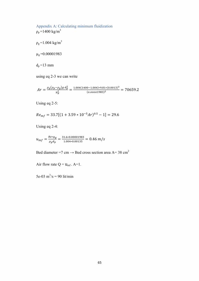
dryer using low temperature air (T≤70 ˚C). Minimum fluidization velocity was
calculated and applied to the experiment. Samples showed poor fluidization
due to large particle size (1-2.8 mm) and density (1400 kg/m3). The effect of
drying parameters was studied experimentally. Gas temperature showed a
great effect on increasing drying rate in the constant drying period and low
effect in the falling rate period. Increasing gas velocity proved to be poorly
effective in drying due to low fluidization. Smaller particle size led to higher
drying rate. Drying curves were curve fitted to available kinetic models in the
literature and logarithmic model showed the best fit. Diffusion coefficient,
activation energy and pre-exponential factor of lignite drying were calculated
and showed good agreement with reported values in the literature. CFD
analysis was carried out in Ansys-Fluent 14.0 and tuning the solid-fluid
exchange coefficient, the constant rate drying period was successfully
simulated. Spontaneous combustion kinetics of Canadian lignite was studied
experimentally and analytically.
iii
Dedicated to my beloved:
“Mother”
….
iv
Acknowledgement
I would like to thank my kind supervisor Dr. Gupta for his guidance
and patience and mention how grateful I am to Dr. Nikrityuk for his support
and help in the course of this thesis.
My gratitude extends to all our group members specially Dr. Mehdi
Mohammad Ali Pour for their help and support.
Finally, I would like to thank C5MPT and department of chemical and
material engineering staff for their cooperation which made this project
possible.
v
List of Figures
Figure 1-1: types of water in coal [15] .......................................................................... 4
Figure 2-1: pressure drop vs. fluid velocity for packed and fluidized beds [23] ........ 10
Figure 3-1: Fluidized bed setup for coal cleaning [49] ............................................... 20
Figure 3-2: Fluidized bed ............................................................................................ 20
Figure 4-1: weight vs. time plots of 1-1.7 mm size under 90 lit/min for 100 gr of
samples ........................................................................................................................ 22
Figure 4-2: weight loss% vs. time plot for 1-1.7 mm size under 90 lit/min for 100 gr
sample ......................................................................................................................... 22
Figure 4-3: drying rate vs. X (gr water/gr dry coal) .................................................... 24
Figure 4-4: weight vs. time for 1-1,7 and T=50 ˚C at different air flow rates ............ 25
Figure 4-5: Moisture reduction % vs time for 1-1.7 mm size at 50 C under different
air flow rate ................................................................................................................. 25
Figure 4-6: drying rate vs. X for 1-1.7 mm at 50 ˚C for different gas flow rates ....... 26
Figure 4-7: weight vs. time in T=50 ˚C and Q=90 lit/min .......................................... 27
Figure 4-8: drying rate vs X % at T=50 °C and Q=90 lit/min .................................... 27
Figure 4-9: weight vs time curve for 1-1.7 mm .......................................................... 28
Figure 4-10: drying rate vs. X % at 70 C .................................................................... 28
Figure 4-11: weight vs. time for different drying conditions of 1-1.7 mm size .......... 30
Figure 4-12: X vs. time for 1-1.7 mm dried in 70 C and 90 lit/min and diffusion fit . 31
Figure 4-13: X vs. time for 1-1.7 mm dried in 70 C and 90 lit/min and logarithmic fit
.................................................................................................................................... 31
Figure 4-14: plot of ln MR vs time for dp=1-1.7, T=70 °C, Q=90 lit/min, ................. 34
Figure 4-15: Ln MR vs. time for t=0-900 sec, T=70 ˚C , Q=90 lit/min ...................... 35
Figure 4-16: Ln MR vs. time fort=900-1750 sec, T=70 ˚C, Q=90 lit/min .................. 36
Figure 4-17: weight vs. time for T=70 ˚C, Q=90 lit/min and dp=1-1.7 mm ............... 38
Figure 4-18: weight vs time for different drying conditions and fitted linear curves . 39
Figure 4-19: natural logarithmic plot of k vs. 1/T ....................................................... 43
vi
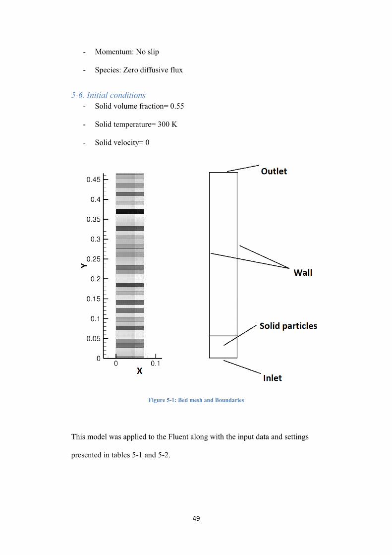
Figure 5-1: Bed mesh and Boundaries ........................................................................ 49
Figure 5-2: solid volume fraction in the first 1.13 sec using Syamlal-Obrein Drag
model .......................................................................................................................... 51
Figure 5-3: solid volume fraction calculated by tuned Syamlal-Obrein drag model .. 52
Figure 5-4: mass flux vs. time of H2O at the outlet for T=20 ˚C and 70 ˚C ............... 53
Figure 6-1: TGA-DSC signal of 2 C/min test ............................................................. 54
Figure 6-2: weight loss derivative of dried samples at 0.4, 1, 2 ˚C/min ..................... 55
Figure 6-3: ln rate vs. 1/T at conversion of 0.5 ........................................................... 57
vii
List of Tables
Table 1-1: top 10 brown coal producers of 2013 [1] .................................................... 1
Table 2-1: approximate ranges of moisture content of coal required for various
processes [17] ............................................................................................................... 6
Table 3-1: Proximate analysis of Boundary Dam coal ............................................... 19
Table 4-1: thin layer equations suggested in the literature [29] .................................. 30
Table 4-2: fitting equations and calculated coefficients for different drying conditions
.................................................................................................................................... 32
Table 4-3: diffusion coefficient for different drying conditions ................................. 36
Table 4-4: mass transfer coefficients for different drying conditions ......................... 37
Table 4-5: results of cA2 and NA for different drying conditions................................. 40
Table 4-6: Mass flux of water leaving the bed calculated by Stefan approach ........... 41
Table 4-7: corrected Stefan values and experimental values for mas flux.................. 42
Table 4-8: k and ln (k) values of each temperature for 1-1.7 mm size and 90 lit/min
gas flow rate ................................................................................................................ 43
Table 4-9: k values taken from diffusion curve fitted to the experimental results...... 44
Table 5-1: Input parameters for Fluent ....................................................................... 50
Table 5-2: Solver Spatial discretization ...................................................................... 50
Table 6-1: kinetic values of combustion in different heating rates ............................. 56
Table 6-2: thermodynamic and kinetic of dried coal .................................................. 57
viii
Table of Contents Chapter 1: Introduction ................................................................................................. 1
1-1. Coal structure and formation ............................................................................ 1
1-2. Canada’s coal reserves ..................................................................................... 2
1-3. Importance of lignite upgrading ........................................................................ 2
1-4. Types of water in coal ........................................................................................ 4
1-5. Scope of the study .............................................................................................. 5
Chapter 2: Literature review ......................................................................................... 6
2-1. Necessity of coal drying ..................................................................................... 6
2-2. Coal drying methods .......................................................................................... 7
2-2-1. Evaporating drying .................................................................................... 7
2-2-1-1. Rotary drum steam tube dryer ................................................................ 7
2-2-1-2. Integrated flash mill drying systems ....................................................... 7
2-2-1-3. Fluidized bed dryer ................................................................................. 8
2-2-2. Non-evaporating drying ............................................................................. 8
2-2-2-1. Fleissner Process .................................................................................... 8
2-2-2-2. Hydrothermal dewatering ....................................................................... 8
2-3. Fluidized bed ..................................................................................................... 9
2-3-1. Fluidization definition ................................................................................ 9
2-3-2. advantages and disadvantages ................................................................. 10
2-3-3. Geldart Powder classification .................................................................. 10
2-3-4. Fluidized bed equations............................................................................ 11
2-3-4-1. bed pressure drop ................................................................................. 11
2-3-4-2. Minimum fluidization velocity ............................................................... 12
2-4. Drying kinetics ................................................................................................. 13
2-4-1. Effect of drying parameters ...................................................................... 13
2-4-2. Modeling Kinetics .................................................................................... 14
2-5. CFD modeling ................................................................................................. 16
2-6. Coal spontaneous combustion ......................................................................... 17
Chapter 3: Setup and Experiments .............................................................................. 19
3-1. Material ........................................................................................................... 19
3-2. Material density measurement ......................................................................... 19
3-3. Fluidized bed setup and procedure ................................................................. 20
3-4. Thermogravimetric procedure ......................................................................... 21
ix
Chapter 4: Results and discussion ............................................................................... 22
4-1. Effect of drying conditions on drying rate in Fluidized bed ............................ 22
4-1-1. Effect of inlet gas temperature ................................................................. 22
4-1-2. Effect of gas inlet rate .............................................................................. 24
4-1-3. Effect of particle size ................................................................................ 26
4-2. Lignite drying using thermogravimetric method ............................................. 28
4-3. Mathematical modeling of drying of lignite in fluidized bed ........................... 29
4-4. Calculating the mass transfer rate kc .............................................................. 33
4-4-1. Diffusion coefficient ................................................................................. 33
4-4-2. Mass transfer coefficient .......................................................................... 36
4-4-3. Mass flux .................................................................................................. 37
4-4-4. Mass transfer coefficient using Stefan problem approach ....................... 40
4-5. Calculating the activation energy of drying .................................................... 42
Chapter 5: CFD modeling of lignite drying in a fluidized bed ................................... 45
5-1. Introduction ..................................................................................................... 45
5-2. CFD Multiphase Models ................................................................................. 45
5-2-1. The Euler-Lagrange approach ................................................................. 45
5-2-2. The Euler-Euler approach........................................................................ 46
5-2-2-1.The VOF ................................................................................................. 46
5-2-2-2.The mixture ............................................................................................ 46
5-2-2-3.The Eulerian ........................................................................................... 46
5-3. Equations for Eulerian model .......................................................................... 46
5-4. Syamlal-O’brein Drag model .......................................................................... 47
5-5. Boundary conditions ........................................................................................ 48
5-6. Initial conditions .............................................................................................. 49
5-4. Tuned Syamlal-Obrein model .......................................................................... 51
Chapter 6: Spontaneous combustion of lignite ........................................................... 54
Chapter 7: Summary and Conclusion ......................................................................... 58
7-1. Summary .............................................................................................................. 58
7-2. Conclusion ........................................................................................................... 59
Appendix A: Calculating minimum fluidization ........................................................ 65
1
Chapter 1: Introduction
1-1. Coal structure and formation
Coal is an organic composition of mainly carbon, oxygen and hydrogen. It is a
fossil fuel which with almost 109 years of remaining in the whole world is far
more abundant than oil and gas. While it can be found in almost all countries,
the largest reserves include the US, Russia, China and India. Over 6185
million tonnes (Mt) of hard coal and 1042 Mt of brown coal/ lignite is
currently produced worldwide. Coal is formed by the consolidation of
vegetables between rocks under pressure and heat over millions of years [1].
Lignite (brown coal) is the lowest rank of coal because of having a low
heating value and high moisture content. This low energy density and
relatively high moisture content makes it economically inefficient to transport,
thus, mostly burnt in power plants situated near the area where it is mined [2].
However in future, lignite can have other applications because of some
advantages it has over black coal; including low mining cost, high volatile
content and reactivity and low mineral matters such as sulfur and nitrogen [3].
China, Germany, Russia, Australia, the US and Canada are among countries
mining lignite [2]. Table 1-1 shows the top 10 Brown coal producers of 2013.
Table 1-1: top 10 brown coal producers of 2013 [1]
Germany 183 Mt Australia Germany
Russia 73 Mt Greece Russia
USA 70 Mt India USA
Poland 66 Mt Czech Republic Poland
Turkey 63 Mt Serbia Turkey
2
1-2. Canada’s coal reserves
In Canada, with 6.6 billion tonnes of recoverable reserves, coal is certainly the
most abundant fossil fuel. Types of Canada’s coal deposits include bituminous
coal, sub-bituminous coal, lignite and anthracite. West provinces contain more
than 90 % of the coal deposits which along with the oil-sand deposits and
access to the west coast ports, provide a great advantage for the country.
Canada has 24 coal mines in total which are in British Colombia, Alberta,
Saskatchewan and Nova Scotia [4]. In Alberta, coal mining in started in 1800s.
The province contains 70 % of the country’s coal deposits. Alberta spends
more than 25 million tonnes of coal for electricity generation annually.
Alberta coal has low sulphur content and thus produces less pollutants
compared to many other coals around the world [5].
1-3. Importance of lignite upgrading
In comparison to bituminous coal, lignite burning power plants have lower
efficiency which is due to high moisture content of lignite. When wet coal is
burnt in a power plant, a large portion of the fuel’s heat input (20-25%) is
spent on evaporating the water contents [6], which reduces the plant efficiency
significantly. High moisture also increases the transportation costs as well as
stack flue gas flow rate and the risk of spontaneous combustion [3].
Apart from the economic issues of burning low rank coal, a number of
environmental issues arise when using coal as a fuel. Coal is a major source of
releasing greenhouse gases (GHG) and toxic minerals to the atmosphere. The
greenhouse gases emitted by coal burning power plants include Carbon
Dioxide (CO2), Carbon Monoxide (CO) and Methane (CH4) [7]. At present the
CO2 produced by burning lignite for generating a MWh electricity is one third
3
more than that of black coals [6]. If coal moisture content is reduced from
60% to 40%, a relative reduction of 30% in the CO2/MWh will be resulted [8].
These environmental issues have motivated researchers and industries to look
for alternatives for coal and other fossil fuels. Innovative techniques and
materials like biomass were suggested, but high production and installation
costs, as well as maintenance expenses are barriers stopping investors from
applying these new technologies. This signifies the importance of producing
low moisture clean coal to feed power plants which are environmental friendly
[9].
Countries with largest lignite reserves like Germany, Australia and the U.S
are the pioneers in searching for effective coal-dewatering and drying
techniques [10].
The amount, distribution and type of bounding of water in coal are factors
determining the ease of its removing from coal. Coal matrix is composed of
small and large capillaries which control the transport of the gases (water,
oxygen etc.) through it [11]. Understanding the characteristics of the coal
which is to be dried is the key factor in choosing the right technique and
designing efficient setup for water removal.
The majority of the developed techniques use high-grade heat to dry coal or
require complex and expensive equipment, increasing the cost of thermal
drying, and thus preventing the application of these techniques in large
industrial scales [12].
Moreover, use of carbon capture technology at power plants which burn low-
rank, high-moisture coals signifies the need for efficient, inexpensive coal
4
drying methods to recover a portion of the efficiency loss due to the
compression of carbon dioxide (CO2), so that, future power plants, employing
CCS, would benefit from thermally dried coal [12].
1-4. Types of water in coal
The nature and type of water and its boundings in coal have been studied in
the literature and different classifications have been suggested. It is widely
accepted that water can be as a free or bound phase in coal [13]. In the primary
researches, water in coal was classified as freezable and non-freezable.
Freezable water was the larger fractions of water in the coal structure which
was able to crystallite and create ice, while non-freezable water referred to
adsorbed water on the internal surfaces or the water in small pores which was
incapable of creating crystal ice [14]. Another classification by (Allardic and
Evans 1971) suggested 2 types of water in coal: chemically adsorbed water
which can only be removed by temperature increase and thus thermal
decomposition, and water which can be removed by evacuation. Increasing the
temperature will result in progressive removal of the first moisture type.
Figure 1-1: types of water in coal [15]
5
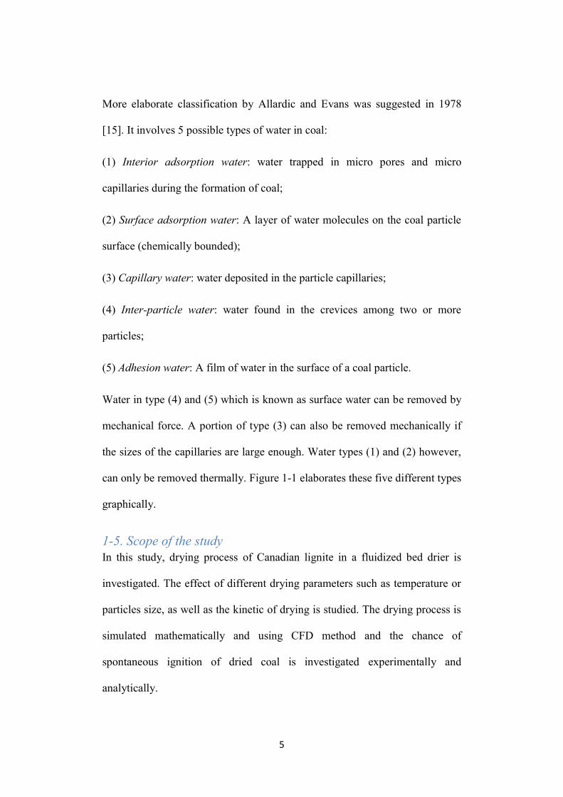
More elaborate classification by Allardic and Evans was suggested in 1978
[15]. It involves 5 possible types of water in coal:
(1) Interior adsorption water: water trapped in micro pores and micro
capillaries during the formation of coal;
(2) Surface adsorption water: A layer of water molecules on the coal particle
surface (chemically bounded);
(3) Capillary water: water deposited in the particle capillaries;
(4) Inter-particle water: water found in the crevices among two or more
particles;
(5) Adhesion water: A film of water in the surface of a coal particle.
Water in type (4) and (5) which is known as surface water can be removed by
mechanical force. A portion of type (3) can also be removed mechanically if
the sizes of the capillaries are large enough. Water types (1) and (2) however,
can only be removed thermally. Figure 1-1 elaborates these five different types
graphically.
1-5. Scope of the study
In this study, drying process of Canadian lignite in a fluidized bed drier is
investigated. The effect of different drying parameters such as temperature or
particles size, as well as the kinetic of drying is studied. The drying process is
simulated mathematically and using CFD method and the chance of
spontaneous ignition of dried coal is investigated experimentally and
analytically.
6
Chapter 2: Literature review
2-1. Necessity of coal drying
Coal is a cost-effective fuel for power plants and industries due to its high
abundance and low cost. Around 45 % of the world’s coal reservoirs consist of
lignite, a cheap coal type, low in sulfur but high in moisture (25-40%),
resulting in a low calorific value compared to other coal types [16], [17]. Great
tendency for spontaneous combustion, and high transportation costs are other
disadvantages of lignite, making it undesirable for industrial processes.
Moisture reduction can increase the quality and efficiency of coal to a
desirable amount for different processes. However, due to high amount of
moisture in lignite, drying requires a large amount of energy [17]. Table 2-1
shows the approximate ranges of moisture content of coal for different
processes.
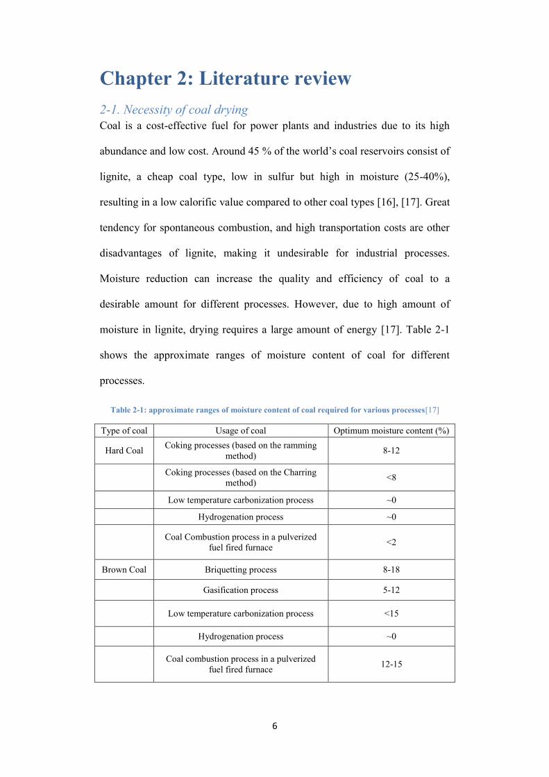
Table 2-1: approximate ranges of moisture content of coal required for various processes[17]
Type of coal Usage of coal Optimum moisture content (%)
Hard Coal Coking processes (based on the ramming
method) 8-12
Coking processes (based on the Charring
method) ˂8
Low temperature carbonization process ~0
Hydrogenation process ~0
Coal Combustion process in a pulverized
fuel fired furnace ˂2
Brown Coal Briquetting process 8-18
Gasification process 5-12
Low temperature carbonization process ˂15
Hydrogenation process ~0
Coal combustion process in a pulverized
fuel fired furnace 12-15
7
2-2. Coal drying methods
Drying is defined as reducing the water content of coal to a desired level. This
can be done through (i) evaporating drying or (ii) non-evaporating drying.
2-2-1. Evaporating drying
When the water content of the coal is transferred into gas phase to be
removed, the process is called evaporating drying [10]. This method mostly
uses superheated steam, hot air or combustion gases. Typical dryers working
based on this principle include: fixed and fluidized beds, rotary kiln and
entrained systems [17]. Generally, in the evaporative drying methods, Coal is
introduced into a rotary vessel where superheated steam is applied. The
discharged steam is partially condensed, just enough to subtract the added
water by the drying process, with the remaining steam being reheated to enter
the cycle again [10]. Besides increasing thermal efficiency of coal, this
method reduces the risk of spontaneous combustion of coal by decreasing coal
reactivity in the presence of oxygen [18].
2-2-1-1. Rotary drum steam tube dryer
This evaporating drying technique is currently used by industries in Germany
and India. It includes a steam drum with coal passing through the tubes inside
the drum. This method reduces the risk of fire by dried coal significantly [10].
2-2-1-2. Integrated flash mill drying systems
This method is used for ground brown coals. The brown coal is crushed into
powder in a “beater” mill and is exposed to hot flow gas. The gas is then
recycled from the furnace exit. In another similar technology, the gas
temperature is increased by burning some coal or natural gas and then is fed to
the mill [10].
8
2-2-1-3. Fluidized bed dryer
Fluidized beds consist of a bed of particles exposed to an upward pressurized
fluid which results in particles showing fluid-like behaviour. They are widely
used in food and other industries dealing with granular solids [19].
2-2-2. Non-evaporating drying
Non-Evaporating drying includes methods distracting water in coal by
applying pressure and mechanical forces. Examples include: Fleissner Process,
K-Fuel, mechanical thermal expression (MTE) and hydrothermal dewatering
(HTD). These methods mainly use heat and pressure to increase the heat value
of coal and reduce impurities such as mercury and sulfur dioxides and nitrogen
oxides in coal physically and chemically [10][17].
2-2-2-1. Fleissner Process
In this process lump coal particles, without being crushed into smaller sizes,
can be economically dried. Coal lumps are placed in a batch autoclave and
heated in 180-240 °C steam under 400 pounds of pressure. The steam
carrying the moisture leaves the dryer and the remaining moisture is removed
using a vacuum pump. The dried lump contains less than 10 % moisture and a
heating value of 10000 Btu/pound. It can be ground to powder form easily and
even burns efficiently in the lump form. Several industries in Europe use this
technique [10].
2-2-2-2. Hydrothermal dewatering
Hydrothermal dewatering is a process in which coal is heated up under
pressure to temperatures above 180 °C. In such process physical and chemical
mechanisms release an increasing amount of water from coal. In hydrothermal
dewatering hot water, instead of steam, is utilised as the heating medium. The
9
pressure is kept high enough to make sure water in coal remains in the liquid
form [20].
2-3. Fluidized bed
Fluidized beds are widely used in different industrial processes including
drying, cooling, granulation, coating etc. They can be used for both heat
sensitive and non-heat sensitive materials. In coal industry, fluidized beds are
used in processes such as drying, gasification and de-volatilization. Fluidized
bed dryers (FBD) are useful for drying powders, granulates, agglomerates, and
pellets in the size range of 50 to 5000 µm. Particles out of this size range are
either too small or too big to fluidize and may require additional forces, i.e.
vibration, to fluidize[21], [22].
2-3-1. Fluidization definition
When an upward fluid is passed through a bed of particles, due to the
frictional forces between the fluid and the particles, fluid pressure will
decrease. Increasing the fluid flow will increase the pressure drop up to a
certain point where a small reduction in the pressure drop is observed (figure
2-1). For air superficial velocities larger than that no more increase in the
pressure drop will be observed. The velocity at which the pressure drop stops
increasing is called the minimum fluidization velocity, where the drag force
applied to the particles will be equal to the apparent weight of the particles.
This leads to particles being lifted slightly by the fluid and the bed is
considered fluidized [23].
10
Figure 2-1: pressure drop vs. fluid velocity for packed and fluidized beds [23]
2-3-2. advantages and disadvantages
Some of fluidized bed advantages are:
- high surface area contact between solid and fluid particles
- Quick heat and mass transfer between solid and fluid particles
- Fast particle mixing
- Low maintenance cost [24], [19], [9].
And a few disadvantages include:
- Not sustainable for particles with low sphericity or wide particle size
range [17]
- Solid particle erosion due to solid-solid and solid-wall collisions
- Back mixing [25]
To overcome the disadvantages of fluidized beds, several solutions have been
proposed. Installing mechanical vibration to the fluidized bed dryer is one of
the solutions which increases the uniformity of the process and has been
accepted and used by industries [24].
2-3-3. Geldart Powder classification
Geldart (1973) classified materials in terms of their fluidization behaviour into
four categories:
Group A:
Materials with a small mean size (less than 30 µm) and/or low density (less
than 1.4 g/cm3) are classified in this group. They are easily fluidized and
11
slowly collapse when the gas supply is cut off. Face centred cubic catalysts
are among this group.
Group B:
This group contains materials in size range of 40-500 µm with a density in
range of 4-1.4 g/m3. Bed expansion is small in this group and it collapses
immediately when the air supply is cut off. Bubbles will be formed at air
supply velocities a little above fluidization. Sand is the most typical example
of this group.
Group C:
Cohesive fine powders belong to this group. Fluidizing this group of materials
is very difficult because they lift in plugs of small channels due to their inter-
particle attractions being greater than the force applied by the fluid. Flour and
cosmetic powders belong to this group.
Group D:
Very large or very dense materials belong to this group. Fluidizing this group
is difficult and solid particle mixing is quite poor. Vegetable grains such as
bean and coal (including lignite) belong to this group of powders.[9][26]
2-3-4. Fluidized bed equations
2-3-4-1. bed pressure drop
As explained above, fluidization happens when the upward drag force applied
on particles from the fluid equals the apparent weight of particles. Righting the
force balance in this situation leads to:
Fluid pressure drop across the bed =𝑝𝑎𝑟𝑡𝑖𝑐𝑙𝑒 𝑤𝑒𝑖𝑔ℎ𝑡 − 𝑢𝑝𝑡ℎ𝑟𝑢𝑠𝑡 𝑜𝑛 𝑝𝑎𝑟𝑡𝑖𝑐𝑙𝑒𝑠
𝑏𝑒𝑑 𝑐𝑟𝑜𝑠𝑠 𝑠𝑒𝑐𝑡𝑖𝑜𝑛 𝑎𝑟𝑒𝑎
Or 𝛥𝑝 =𝐻𝐴(1−𝜀)(ρp−ρg)𝑔
𝐴= 𝐻(1 − 휀)(ρp − ρg)𝑔 (2-1)
12
Where:
H: bed height in (m)
A: bed cross section area (m2)
ρp: Particle density in (kg/m3)
ρf: Fluid density in (kg/m3)
ε: Bed voidage (dimensionless)
Knowing the bed voidage and particle and gas properties the pressure drop can
be calculated.
2-3-4-2. Minimum fluidization velocity
Minimum fluidization velocity Umf is the air supply superficial velocity at
which the fluidization occurs. Below this velocity a packed bed is obtained
and above that bubbling or spouting bed is reached. Umf increases with particle
size and density as is directly affected by the fluid properties [23].
To write an expression for the Umf we can equate the pressure loss equation of
a fluidized bed (equation 1) with that of a packed bed. Using this method and
taking some assumptions Wen and Yu (1966) produced an equation in the
form of:
𝐴𝑟 = 1652𝑅𝑒𝑚𝑓 + 4.51𝑅𝑒𝑚𝑓1 (2-2)
In equation 2-2, Ar is the dimensionless number known as Archimedes
number defined as:
𝐴𝑟 =𝜌𝑔(𝜌𝑝−𝜌𝑔)𝑔 𝑑𝑝
3
µ𝑔2 (2-3)
And Remf is the Reynolds number at the fluidization velocity:
𝑅𝑒𝑚𝑓 =𝑈𝑚𝑓𝜌𝑔𝑑𝑝
µ𝑔 (2-4)
Wen and Yu correlation can also be expressed in the form:
13
𝑅𝑒𝑚𝑓 = 33.7[(1 + 3.59 ∗ 10−5𝐴𝑟)0.5 − 1] (2-5)
Valid for spheres larger than 100 µm in the Remf range of 0.01-1000 [23].
For particles smaller than 100 µm Beayens and Geldart correlation (1974) can
be used:
𝑈𝑚𝑓 =(𝜌𝑝−𝜌𝑓)
0.934𝑔0.934𝐷𝑝
1.8
1110µ0.87𝜌𝑓0.066 (2-6)
2-4. Drying kinetics
Studying drying kinetics and characteristics of coal provides important data to
be able to pick the most efficient drying technique with the optimum setup
built based on that technique. Before employing the setup in the industrial
scale, a laboratory scale setup and analysis is required to characterize the
whole process under a well- controlled environment [27].
2-4-1. Effect of drying parameters
Vorres [28] and Tahmasebi et al [29] used a thermogravimetric analyzer to
study the drying behavior of Wyodak subbituminous coal and Chines lignite
respectively. Vorres included that the rate of moisture removal in the sample is
affected by the drying temperature, inlet gas flow rate and the sample size.
Wang et al [30] reported that if the air flow temperature is increased with a
constant rate, weight loss will show a sharp decrease in the first minutes, and
then a gradual decrease will be observed till the end of the experiment. Zhao et
al [24] investigated the effect of drying conditions on a vibration fluidized bed
and concluded that higher frequency and lower bed height were favorable for
drying.
14
2-4-2. Modeling Kinetics
C.Srinivasakannan and N.Balasubramanian suggested a simplified equation to
model the constant rate period of drying in a batch fluidized bed. The model
divides the bed into dense and bubble phases. Using the characteristics of the
materials and the bed shape, it predicts the drying rate of the constant rate
period. They compared the predicted drying rate with the experimental results
of different materials in different conditions (gas velocity, solid hold-up, bed
shape and diameter etc.) and found that the model is in satisfactory agreement
with experimental data [31].
Chandran et al [32] introduced a simple model to predict both the constant and
falling rate of drying in a fluidized bed. They assumed that the falling rate is
linear with starting point at the critical moisture content and ending point at
the equilibrium moisture content. Their model predicts the moisture content of
the bed material at any time by knowing the initial, critical and equilibrium
moisture content as well as the drying rate coefficient R, which is expressed as
the weight of water evaporated per unit weight of dry solid.
Edward K. Levy et al [33] studied the drying of coal in a bubbling fluidized
bed. They used the conservation of mass and energy and wrote an ODE for
coal moisture and bed temperature as a function of time. Solving the ODE
numerically and comparing the results with the experiment results of a high
moisture sample in the bed, showed good agreement between the two sets of
data.
Ciesielczyk et al [34] assumed that heat delivered to the particle is entirely
used to remove the moisture and the particle surface is completely covered
with the moisture. They also assumed that moisture removal only occurs at the
15
external surface of the particle and that the temperature of the particle is the
wet bulb temperature. They wrote an expression for the drying rate as a
function of dry solid mass, specific surface area, solid holdup, concentration
gradient and mean mass transfer coefficient. To calculate the mean mass
transfer coefficient they used the bubbling bed model.
Syahrul, S et al [35] studied mass, energy and entropy balance of fluidized bed
dryers with corn and wheat particles. They studied the thermal efficiency of
the bed under different drying conditions such as initial moisture content of
the particles, air flow rate etc.
Cai et al [36] presented a general empirical kinetic model for solid state
reactions. Their proposed model is f(𝛼) = 𝛼𝑚(1 − 𝑞𝛼)𝑛 (m and n are
empirical coefficients), where α is the conversion degree in the form of:
𝛼 =𝑊𝑖−𝑊
𝑊−𝑊𝑓 (2-7)
Where:
Wi: initial weight of solids
W: weight of solid at any time
Wf: final weight of solid at the end of the reaction
And f(α) is the kinetic model in differential form. They showed that other
kinetic models in the literature can be fitted with their model by calculating
proper values for m, n and q in each case. Kang et al [37] studied these kinetic
models validity in predicting isothermal and non-isothermal drying of
Indonesian coal and concluded that phase boundary reaction in the form of
f(α) =1- (1- α)1/3
was the best fit for drying Indonesian coal mechanism in an
isothermal fixed be reactor.
16
Burgschweiger et al [38] studied the drying kinetics of a single particle as well
as a bubbling fluidized bed of the particles. They believed batch fluidized bed
drying curves could be predicted using the single particle and material
equilibrium data and their developed model. They derived their model by
writing mass and energy balance for the suspension gas and bubbles as well as
energy balance for the bed walls. They used van Meel normalization approach
but defined a modified normalized drying rate with a mass flux with a sorptive
driving force term. Their model coped well with experimental data of single
particle drying and batch fluidized bed drying.
Tahmasebi et al [29] and studied lignite drying kinetics using
thermogravimetric method. Using the data obtained from the experiment they
calculated the apparent diffusion coefficient and activation energy of drying
lignite. Mirzaee et al [39]used the same method for drying of apricot in a
packed bed.
2-5. CFD modeling
CFD modeling is a very useful numerical method to help optimize processes
and improve energy efficiency of industrial cycles [40].
Azizi et al [41] used CFD method to model a spouted bed of glass particles.
They used multiphase Eulerian-Eulerian approach based on kinetic theory and
using Gidasow’s drag model for predicting gas-solid momentum exchange.
They studied the effect of solids mass fraction as well as gas flow rate on the
distribution of pressure along the spouted bed.
Roman et al [40] used CFD to study heat and mass transfer for drying of
grains in a spouted bed. They used Eulerian-Eulerian approach and the applied
17
heat and mass transfer models using user defined files (UDF) to Fluent 6.1.
They concluded that their model predicts mass transfer, Nusselt and Sherwood
number accurately but is poorly successful in predicting heat transfer.
Jamaleddine and Ray [42] studied drying of sludge in a cyclone dryer using
CFD analysis. They wrote a UDF to simulate constant and falling rate drying
periods. The hydrodynamics analysis showed a nun-uniform particle
distribution across the dryer. Moisture content, temperature, and velocity were
monitored and the model showed a good degree of success in predicting the
process.
2-6. Coal spontaneous combustion
Spontaneous combustion of coal has been a serious problem for coal
producers and users industries [43]. This phenomenon can result in disastrous
economic losses and casualties. Spontaneous combustion happens due to the
low temperature oxidation of coal particles. As this process is exothermic, if
proper ventilation is not provided, the coal temperature can increase to a point
when combustion occurs [44].
Yongliang et al [45] calculated the shortest period of coal spontaneous
combustion on the basis of oxidation heat release and coal thermal capacity at
different temperatures. They showed that the shortest spontaneous combustion
period increases when oxidation absorption is decreased and the activation
energy is increased.
Qi et al [46] used DSC experiments to observe the heat behaviour of coal to
determine the kinetic parameters and predict the oxidation process. Their
study successfully predicted temperature profile of coal in the self-heating
18
process. Zhao et al [47] used the same DSC instrument as Qi et al and
measured activation energy of spontaneous combustion for cotton. Using the
Semenov model, they calculated the self-heating oxidation temperature
(SHOT) of cotton in different heating rates.
In this study, data obtained from fluidized bed dryer is analyzed using the
same apparent diffusion approach used by Tahmasebi [29] and Mirzaee [39].
This method uses the conversion and time data and does not require coal
particles temperature which is difficult to measure during the experiments in
the bed. CFD modeling is carried out to model the drying process using a
constant rate input, and spontaneous combustion risk of Canadian lignite is
studied in a TGA-DSC with the same approach as Zhao [47] and Qi [46].
19
Chapter 3: Setup and Experiments
3-1. Material
The coal sample used in this study is Boundary Dam lignite. Samples were
sieved and kept sealed before and after experiments. The proximate analysis of
Boundary Dam coal was measured using a Leco TGA701 thermogravimetric
analyzer and is presented in table 3-1.
Table 3-1: Proximate analysis of Boundary Dam coal
Fixed carbon% Moisture % Volatile
matter% Ashe%
23.4 21 40.5 13.4
3-2. Material density measurement
The particle density used in fluidized beds is the apparent density defined as
particle mass divided by its hydrodynamic volume. This volume is the one
seen by the fluid and includes the particle and its open and close pores. This
density is different from the absolute density which accounts for the real
volume of the particle (apparent volume minus the pores). Measuring the
apparent density of porous materials is not an easy procedure because
common methods measure the absolute density [23]. In this study the apparent
density of coal samples was measured using water displacement method [48].
A bottle of known weight was filled with an amount of water with measured
weight. A small number of coal particles were weight measured and added to
the bottle. The change in the water level was written down immediately,
before water diffuses into the particles pores. The measured density for
Boundary Dam coal was 1400 kg/m3.
20
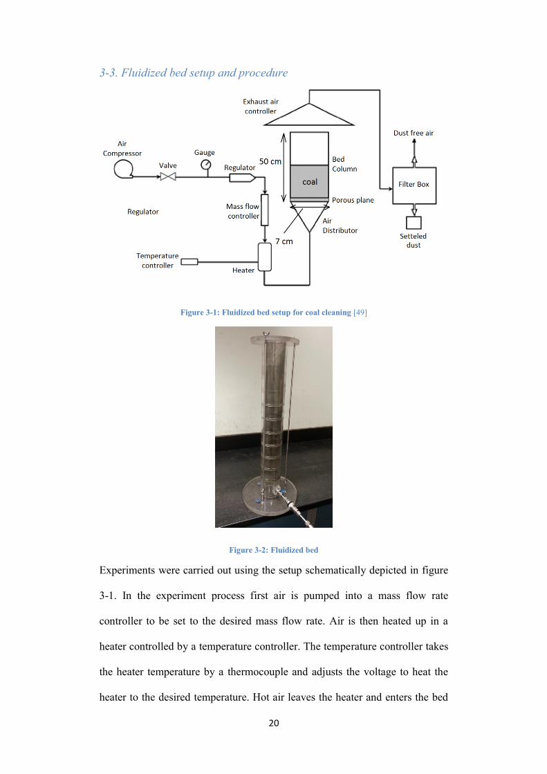
3-3. Fluidized bed setup and procedure
Figure 3-1: Fluidized bed setup for coal cleaning [49]
Figure 3-2: Fluidized bed
Experiments were carried out using the setup schematically depicted in figure
3-1. In the experiment process first air is pumped into a mass flow rate
controller to be set to the desired mass flow rate. Air is then heated up in a
heater controlled by a temperature controller. The temperature controller takes
the heater temperature by a thermocouple and adjusts the voltage to heat the
heater to the desired temperature. Hot air leaves the heater and enters the bed
21
through a porous distributer to keep the air flow uniform across the bed
entrance. After the desired temperature is reached, a certain amount of coal is
introduced to the bed and the experiment starts. The air flow rate is stopped at
certain time intervals and the weight of the whole bed is measured using a
microbalance. The experiment continues until no significant change is
observed in the bed weight. Subtracting the weight of the empty bed from the
measured weight values, the mass of samples in the bed is calculated at each
time interval.
3-4. Thermogravimetric procedure
Lignite samples were tested in a Leco TGA701 thermogravimetric analyzer
for 10 hours. Air with a flow rate of 7 ml/min was continuously purged into
the instrument chamber at isothermal conditions. Samples weight was
measured and recorded constantly during the experiments.
22
Chapter 4: Results and discussion
4-1. Effect of drying conditions on drying rate in Fluidized bed
4-1-1. Effect of inlet gas temperature
In order to investigate the effect of the inlet gas temperature on the drying
behavior of Boundary Dam coal, tests with Tair=20 °C and Tair=50 °C and
Tair =70 °C were carried out in the bed. The sample size was 1-1.7 mm, the
mass of input sample was 100 gr (±5 %) and the initial moisture
was 21 % (g of water /g of wet coal) with air flow rate of 90 lit/min
(corresponding minimum fluidization velocity, see Appendix A). Figures 4-1
and 4-2 show the test results.
Figure 4-1: weight vs. time plots of 1-1.7 mm size under 90 lit/min for 100 gr of samples
Figure 4-2: weight loss% vs. time plot for 1-1.7 mm size under 90 lit/min for 100 gr sample
75
80
85
90
95
100
105
0 20 40 60 80 100 120
we
igh
t (g
r)
time (min)
T=70 ˚C
T=50 ˚C
T=20 ˚C
0
20
40
60
80
100
0 20 40 60 80 100 120
mo
istu
re lo
ss %
time(min)
T=70 ˚C
T=50 ˚C
T=20 ˚C
23
As you can see in the graphs, there is a constant rate drying in the first stage
followed by a falling rate drying. The constant rate drying corresponds to the
removal of surface moisture of the particles which are poorly bound to the
coal particle (water types of 4 and 5 in Allardic classification). When this
moisture is removed a critical moisture content is left and the drying process
enters the falling rate stage. The falling rate coresponds to the removal of the
water inside the capilaries and pores of the particles (water type 3 of Allardic
classification) which can be partially removed by physical treatments. This
water has to diffuse to the surface to be removed by the air flow.
Figure 4-2 shows that air flow temperature directly affects the drying rate of
coal particles in the constant rate stage. Comparing the results of 20 °C air
inlet temperature, where no heat transfer occurs in bed, and the results of
70 °C, we can see that by increasing the drying temperature, moisture removal
increases by around 40 % in the fisrt stage. In this stage higher air temperature
increases evaporation rate and the particle surface temperature, resulting in
higher moisture removal [29]. In the falling rate stage however, were interior
water has to diffuse to the particle surface, temperature is not an effective
parameter becasue the diffusion driving force is the concentration gradient
from inside the particle towards the surface which is a function of particle
moisture content and air moisture. Air moisture content is proven to be zero in
all temperatures and thus, the falling rate stage is not affected by the
temperature change significantly.
24
Figure 4-3: drying rate vs. X (gr water/gr dry coal)
Figure 4-3 shows the drying rate (g of removed water/g of dry coal per
second) versus X (g of water/g of dry coal) for the same tests. It is obvious
that by increasing the drying temperature from 20 °C to 70 °C, maximum
drying rate (occurring in the constant rate period) is increased from around
0.00015 to 0.0004 [(g water)/(g dry coal).(s)] which is around 2.5 times faster.
4-1-2. Effect of gas inlet rate
To investigate the effect of gas inlet flow rate samples of 1-1.7 mm size with
initial moisture of 21 % were tested under Tair=50 °C and different air flow
rates. Air flow rates of 90 lit/min, 70 lit/min and 50 lit/min were applied to the
samples.
0
0.00005
0.0001
0.00015
0.0002
0.00025
0.0003
0.00035
0.0004
0.00045
0 5 10 15 20 25 30
dry
ing
rate
(g/
g.s)
X % (g of water/g of dry coal)
T=70 ˚C
T=50 ˚C
T=20 ˚C
25
Figure 4-4: weight vs. time for 1-1,7 and T=50 ˚C at different air flow rates
Figure 4-5: Moisture reduction % vs time for 1-1.7 mm size at 50 C under different air flow rate
As shown in figures 4-4 and 4-5 the air flow rate doesn’t affect the drying of
coal particles significantly. In 80 minutes of drying, the moisture reduction
difference for the three flow rates is less than 6 %, suggesting the poor effect
of air flow rate in the process. This is because coal particles, belonging to
group D of Geldard classification, hardly show fluidization behavior. When
the gas velocity corresponding to the minimum fluidization (calculated
theoretically in Appendix A) is applied to the coal particles, we can hardly
observe fluidization behavior and what can be seen is that particles mainly
remain in a packed bed settlement due to low sphericity and high density. In
75
80
85
90
95
100
0 20 40 60 80 100 120
we
igh
t (g
)
time (min)
Q=50 lit/min
Q=90 lit/min
Q=70 lit/min
0
10
20
30
40
50
60
70
80
90
100
0 20 40 60 80 100 120
mo
istu
re lo
ss %
time (min)
Q=90 lit/min
Q=70 lit/min
Q=50 lit/min
26
this condition, the upper particles receive more freedom and move slightly
while except for some bubbles, not much movement happens inside the bed. In
this situation, applying a gas flow rate to uniformly expand the bed and keep
particle slightly separated from each other (the fluidization) is not possible. It
can be concluded that if a bubbling and channeling bed is not desired, it is
more economically efficient to keep the gas flow rate lower than the minimum
fluidization velocity. In this study the term “fluidized bed” will be used only
because tests were performed at the theoretical fluidization velocity. Figure 4-
6 shows poor effect of gas flow rate in the bed.
Figure 4-6: drying rate vs. X for 1-1.7 mm at 50 ˚C for different gas flow rates
4-1-3. Effect of particle size
To investigate the effect of particle size on the drying of lignite, two samples
in the size range of 1-1.7 mm and 1.7-2.8 mm were dried in the fluidized bed
under the same temperature and air velocity.
0
0.00005
0.0001
0.00015
0.0002
0.00025
0.0003
0.00035
0.0004
0 5 10 15 20 25 30
dry
ing
rate
(gr
/gr.
s)
X % (gr water/ gr dry coal)
Q=90 lit/min
Q=70 lit/min
Q=50 lit/min
27
Figure 4-7: weight vs. time in T=50 ˚C and Q=90 lit/min
Weight loss vs time plot of the tests is presented in figure 4-7. As shown in the
figure, the smaller size sample dries faster. Smaller particle means larger total
surface area which leads to a higher heat and mass transfer. It is also
accompanied by less thermal resistance and mass transfer resistance inside
particles [29].
Figure 4-8: drying rate vs X % at T=50 °C and Q=90 lit/min
Figure 4-8 is a plot of the drying rate versus X and as expected, shows a lower
final moisture content (equilibrium moisture content) for the smaller sized as
well as a higher drying rate (around 50 % higher than coarse size).
75
80
85
90
95
100
0 20 40 60 80 100
we
igh
t (g
r)
time (min)
1.7-2.8 mm
1-1.7 mm
0
0.00005
0.0001
0.00015
0.0002
0.00025
0.0003
0.00035
0.0004
0 5 10 15 20 25 30
dry
ing
rate
(gr
/gr.
s)
X %(gr water/dry coal %)
1-1.7 mm
1.7-2.8 mm
28
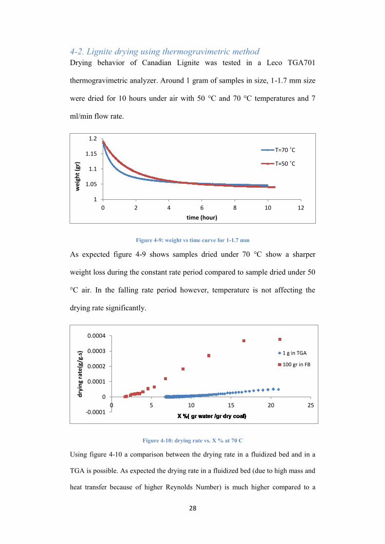
4-2. Lignite drying using thermogravimetric method
Drying behavior of Canadian Lignite was tested in a Leco TGA701
thermogravimetric analyzer. Around 1 gram of samples in size, 1-1.7 mm size
were dried for 10 hours under air with 50 °C and 70 °C temperatures and 7
ml/min flow rate.
Figure 4-9: weight vs time curve for 1-1.7 mm
As expected figure 4-9 shows samples dried under 70 °C show a sharper
weight loss during the constant rate period compared to sample dried under 50
°C air. In the falling rate period however, temperature is not affecting the
drying rate significantly.
Figure 4-10: drying rate vs. X % at 70 C
Using figure 4-10 a comparison between the drying rate in a fluidized bed and in a
TGA is possible. As expected the drying rate in a fluidized bed (due to high mass and
heat transfer because of higher Reynolds Number) is much higher compared to a
1
1.05
1.1
1.15
1.2
0 2 4 6 8 10 12
we
igh
t (g
r)
time (hour)
T=70 ˚C
T=50 ˚C
-0.0001
0
0.0001
0.0002
0.0003
0.0004
0 5 10 15 20 25
dry
ing
rate
(g/g
.s) 1 g in TGA
100 gr in FB
29
drying condition where packed bed of particle are exposed to low air flow rates in
chambers. The maximum drying rate in a fluidized bed is almost 10 times more
which is due to high particle-air contact area leading to faster heat and mass transfer.
4-3. Mathematical modeling of drying of lignite in fluidized bed
Drying is a complex process comprising the heat and mass transfer between a
particle and its surrounding and inside the particle. The movement of moisture
from inside the particle towards the surface and from surface to the
surrounding atmosphere depends on the structure and properties of the drying
material, temperature and moisture concentration of the surrounding
atmosphere and the amount and type of moisture in the particle [50].
Simulating this process provides information for assessment of energy and
time conservation. Simulation is advantageous because real size experiments
of a phenomenon can be time and energy consuming, expensive and even
dangerous.
Mathematical models proposed in the literature include theoretical, semi-
theoretical and empirical equations [50]. Theoretical models are derived from
diffusion equation or simultaneous solving of mass and heat transfer. Semi-
theoretical models are proposed based on Newton’s cooling law which relates
drying rate to the difference between moisture content at each time and the
equilibrium moisture value of the sample [29]. Empirical models use the
experimental data inclusively and suggest mathematical equations fitting the
data.
In this chapter the drying data obtained from the experiment is curve fitted to
some mathematical models introduced in the literature [29].
30
Figure 4-11: weight vs. time for different drying conditions of 1-1.7 mm size
Figure 4-11 presents the weight loss due to moisture removal vs. time for
different drying conditions (temperature and air flow rates) of BD lignite.
Drying starts with a constant rate and continues to a falling rate reaching zero
rate at the end of each experiment. To find the best mathematical model which
fits the process, 4 of the known models in the literature were used for curve
fitting (table4-1).
Table 4-1: thin layer equations suggested in the literature [29]
Model name
Equation
Logarithmic 𝑋 = 𝑎 𝑒𝑥𝑝(−𝑘𝑡) + 𝑏
Diffusion X = 𝑎 𝑒𝑥𝑝(−𝑘𝑡) + (1 − 𝑎)𝑒𝑥𝑝(−𝑘𝑏𝑡)
Simplified Fick 𝑋 = 𝑎 exp (−𝑐(𝑡 𝐿2))⁄
Midilli-Kucuk 𝑋 = 𝑎 exp(−𝑘(𝑡𝑛)) + 𝑏𝑡
75
80
85
90
95
100
0 20 40 60 80 100 120
coal
we
igh
t (g
)
time (min)
T=20 ˚C, Q=90 lit/min
T=50 ˚C, Q=90 lit/min
T=70 ˚C, Q=90 lit/min
T=50 ˚C, Q=50 lit/min
31
The moisture data of sample (X=g water/g dry solid) at each time interval was
plot vs. time and each of the models presented in the table 4-1 was curve fitted
to the data. Regression was carried out using the commercially available data
analyzer Matlab. The package uses the least square algorithm to iterate the
analysis and adjust the parameters.
Figure 4-12: X vs. time for 1-1.7 mm dried in 70 C and 90 lit/min and diffusion fit
Figure 4-13: X vs. time for 1-1.7 mm dried in 70 C and 90 lit/min and logarithmic fit
0 20 40 60 80 100
0.05
0.1
0.15
0.2
0.25
time (min)
X (g
H2O
/g d
ry c
oal)
X vs. time
diffusion
0 20 40 60 80 100
0.05
0.1
0.15
0.2
0.25
time(min)
X (
g H
2O
/g d
ry c
oa
l)
X vs time
logarithmic
32
Table 4-2: fitting equations and calculated coefficients for different drying conditions
Q(lit/min) T(˚C) model coefficients R2 SSE RMSE
90 70
𝑋 = 𝑎 𝑒𝑥𝑝(−𝑘𝑡) + 𝑏 a = 0.2903
k = 0.1486
b = 0.0179
0.996 0.000395 0.004559
90 70
X = 𝑎 𝑒𝑥𝑝(−𝑘𝑡) + (1− 𝑎)𝑒𝑥𝑝(−𝑘𝑏𝑡)
a = 0.7111
b = 0.0220
k = 5.297
0.964
2 0.000352 0.01362
90 70
𝑋 = 𝑎 exp (−𝑐(𝑡 𝐿2))⁄ a =0.2919
c = 0.222
L = 1.37
0.964
2 0.003527 0.01363
90 70
𝑋 = 𝑎 exp(−𝑘(𝑡𝑛)) + 𝑏𝑡 a =3.14
k=0.1635
b=0.00024
n=0.9071
0.991
5 0.000833 0.006805
90 50
𝑋 = 𝑎 𝑒𝑥𝑝(−𝑘𝑡) + 𝑏 a=0.2744
b=0.0192
k=0.09586
0.997
5 0.000460 0.003917
90 50
X = 𝑎 𝑒𝑥𝑝(−𝑘𝑡) + (1− 𝑎)𝑒𝑥𝑝(−𝑘𝑏𝑡)
a=0.7241
b=0.01495
k=4.937
0.975
5 0.004313 0.003984
90 50 𝑋 = 𝑎 exp (−𝑐(𝑡 𝐿2))⁄ a = 0.2778
b = 0.2912
c = 1.978
0.976
9 0.004334 0.01201
90 50
𝑋 = 𝑎 exp(−𝑘(𝑡𝑛)) + 𝑏𝑡 a = 0.2993
b = 0.0002
k = 0.1082
n = 0.9118
0.995
1 0.000917 0.005625
90 20 𝑋 = 𝑎 𝑒𝑥𝑝(−𝑘𝑡) + 𝑏 a = 0.2171
k =0.04059
b =0.06435
0.996
9 0.000534 0.003852
90 20
X = 𝑎 𝑒𝑥𝑝(−𝑘𝑡) + (1− 𝑎)𝑒𝑥𝑝(−𝑘𝑏𝑡)
a = 0.7517
b=0.00497
k = 3.58
0.913
8 0.01464 0.02017
90 20
𝑋 = 𝑎 exp (−𝑐(𝑡 𝐿2))⁄ a = 0.2514
b = 0.1163
c = 2.528
0.911
7 0.01499 0.02041
90 20
𝑋 = 𝑎 exp(−𝑘(𝑡𝑛)) + 𝑏𝑡 a=0.277
b=0.00051
k=0.0306
n=0.9891
0.997
6 0.000414 0.003441
In table 4-2, RMSE stands for the root mean standard deviation, SSE is the
sum of squares due to error and R-square is the coefficient of determination.
Taking R-square as the main fit goodness parameter, the results of curve
fitting shows that logarithmic model seems to be the best model to predict the
drying behavior of lignite in the fluidized bed.
33
4-4. Calculating the mass transfer rate kc
Drying materials in large scale is possible when a prior complete analysis of
the process is available. Physical and thermal properties of the material to be
dried, as well as heat and mass transfer conditions need to be studied. In case
of drying in a fluidized bed, understanding the kinetic parameters is a crucial
data required to design the drier. In this section the diffusion coefficient, mass
transfer coefficient and the activation energy of lignite drying process is
determined from the experimental data.
4-4-1. Diffusion coefficient
Mass diffusion is a type of mass transfer defined as “the movement of a fluid
from an area of higher concentration to an area of lower concentration [51].”
The general equation for the diffusion of the property momentum, heat or
mass in the ɀ direction is [52]:
𝜓ɀ = −𝛿𝑑𝛤
𝑑ɀ (4-1)
Where:
- ψɀ is the flux of the property perpendicular to the area per unit of time
- δ is the diffusion coefficient (m2/s)
- dΓ/dɀ is the driving force (concentration gradient in mass transfer, temperature
difference in heat transfer…) per unit length
For diffusion mass transfer the above equation is expressed in the first Fick’s
law of diffusion as follows:
𝐽𝐴ɀ = −𝐷𝐴𝐵𝑑𝑐𝐴
𝑑ɀ (4-2)
which determines the flux of the diffusion of Material A into B in the direction
of ɀ [52].
34
To calculate the diffusion coefficient for the fluidized bed the following series
proposed by Crank [53] is used:
𝑀𝑅 =𝑀
𝑀°=
8
𝜋2∑
1
(2𝑛−1)∞𝑛=1 exp (−
(2𝑛−1)2𝜋2𝐷𝐴𝐵𝑡
4𝐿2) (4-3)
In this series the MR is the moisture ratio defined as the ratio of the moisture
at each time divided by the initial moisture. M is the moisture content (gr
water/gr dry coal) and M° is the initial moisture content, and L is the thickness
which is the particle radius (rp) in this study.
The first term of the above equation is used for a long drying time [39].
Hence:
𝑀𝑅 =8
𝜋2exp (
𝜋2𝐷𝐴𝐵𝑡
4𝐿2) (4-4)
Taking the Ln of both sides gives:
𝐿𝑛(𝑀𝑅) = 𝐿𝑛 (8
𝜋2) +
𝜋2𝐷𝐴𝐵
4𝐿2𝑡 = 𝑎 + 𝑏𝑡 (4-5)
Plotting Ln (MR) vs. time will give the slop of b. We can write:
𝐷𝐴𝐵 =4𝐿2𝑏
𝜋2 (4-6)
The above equation along with the experimental data can be used to calculate
the diffusion coefficient of lignite particles drying in the fluidized bed.
Figure 4-14: plot of ln MR vs time for dp=1-1.7, T=70 °C, Q=90 lit/min,
-3
-2.5
-2
-1.5
-1
-0.5
0
0.5
0 500 1000 1500 2000 2500 3000 3500 4000
LnM
R
time (sec)
35
Figure 4-14 shows the plot of Ln (MR) vs time for a particle size range of 1-
1.7 mm, in 90 lit/min air flow of 70 °C.
Observing the plot we can see that the curve does not show one linear slope as
expected. Thus we can include that the diffusion coefficient does not remain
constant during the drying and as the particles moisture content reduces, the
diffusion is also decreased.
As discussed in the previous section, in the first 900 seconds of drying, when
the surface moisture is high enough to maintain drying at a constant rate there
is a higher diffusion coefficient (constant rate drying period). As particles
loose surface moisture, the water content inside the capillaries and micro pores
need to be diffused to the surface by overcoming the resistance. This leads to a
reduction in the moisture removal rate and a reduced diffusion coefficient
(falling rate period).
The first and second stages of the process are presented in figures 4-15 and
4-16 with the linear lines fitted to the data.
Figure 4-15: Ln MR vs. time for t=0-900 sec, T=70 ˚C , Q=90 lit/min
y = -0.0023x + 0.1811 R² = 0.997
-1.8-1.6-1.4-1.2
-1-0.8-0.6-0.4-0.2
00.2
0 100 200 300 400 500 600 700 800 900
Ln M
R
time (sec)
36
Figure 4-16: Ln MR vs. time fort=900-1750 sec, T=70 ˚C, Q=90 lit/min
As shown in the figures, the slope of the graph in the first stage is 2.3e-03 and
for the second stage is 0.5e-03. The corresponding diffusion coefficient of the
two stages will be 3.98e-10 m2/s and 0.85e-10 m
2/s. The diffusion coefficient
of other drying conditions is presented in table 4-3. Calculated values are in
good agreement with data in the literature [29].
Table 4-3: diffusion coefficient for different drying conditions
dp(mm) T(˚C) Q(lit/min) b1 D1(m/s) b2 D2(m/s)
1-1.7 70 90 2.3e-03 3.98-10 0.5e-03 0.85-10
1-1.7 50 90 1.2e-03 2.05-10 0.3e-03 0.51e-10
1-1.7 20 90 0.5e-03 0.85e-10 0.2e-03 0.34e-10
1-1.7 50 70 1.2e-03 2.05e-10 0.2e-03 0.34e-10
4-4-2. Mass transfer coefficient
For the Reynolds number in the range of 10-10000, for gases in a packed bed
the correlation for mass transfer is as follows [52]:
𝐽𝐷 =0.4548
𝜀𝑅𝑒−0.4069 (4-7)
y = -0.0005x - 1.421 R² = 0.9712
-3
-2.5
-2
-1.5
-1
-0.5
0
0 500 1000 1500 2000 2500 3000
Ln M
R
time (sec)
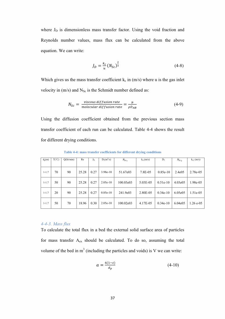
37
where JD is dimensionless mass transfer factor. Using the void fraction and
Reynolds number values, mass flux can be calculated from the above
equation. We can write:
𝐽𝐷 =𝑘𝑐
𝑢(𝑁𝑆𝑐)
2
3 (4-8)
Which gives us the mass transfer coefficient kc in (m/s) where u is the gas inlet
velocity in (m/s) and NSc is the Schmidt number defined as:
𝑁𝑆𝑐 = 𝑣𝑖𝑠𝑐𝑜𝑢𝑠 𝑑𝑖𝑓𝑓𝑢𝑠𝑖𝑜𝑛 𝑟𝑎𝑡𝑒
𝑚𝑜𝑙𝑒𝑐𝑢𝑙𝑎𝑟 𝑑𝑖𝑓𝑓𝑢𝑠𝑖𝑜𝑛 𝑟𝑎𝑡𝑒=
µ
𝜌𝐷𝐴𝐵 (4-9)
Using the diffusion coefficient obtained from the previous section mass
transfer coefficient of each run can be calculated. Table 4-4 shows the result
for different drying conditions.
Table 4-4: mass transfer coefficients for different drying conditions
dp(m) T(˚C) Q(lit/min) Re JD D1(m2/s) 𝑁𝑆𝑐1 kc1(m/s) D2 𝑁𝑆𝑐2 kc2 (m/s)
1-1.7 70 90 25.28 0.27 3.98e-10 51.67e03 7.8E-05 0.85e-10 2.4e05 2.78e-05
1-1.7 50 90 25.28 0.27 2.05e-10 100.03e03 5.03E-05 0.51e-10 4.03e05 1.98e-05
1-1.7 20 90 25.28 0.27 0.85e-10 241.9e03 2.80E-05 0.34e-10 6.05e05 1.51e-05
1-1.7 50 70 18.96 0.30 2.05e-10 100.02e03 4.17E-05 0.34e-10 6.04e05 1.26 e-05
4-4-3. Mass flux
To calculate the total flux in a bed the external solid surface area of particles
for mass transfer Aex should be calculated. To do so, assuming the total
volume of the bed in m3 (including the particles and voids) is V we can write:
𝑎 =6(1−𝜀)
𝑑𝑝 (4-10)
38
Where a is the surface area/total volume of bed with spherical particles
(m2/m
3).
𝐴𝑒𝑥 = 𝑎𝑉 (4-11)
Mass conservation equation can be written as:
𝑁𝐴𝐴𝑒𝑥 = 𝑄(𝑐𝐴2 − 𝑐𝐴1) (4-12)
In the above equations cA1 can be taken as zero (zero inlet air moisture
amount). To calculate the mass transfer rate of the bed plot of weight (g) vs
time (s) can be used.
Figure 4-17: weight vs. time for T=70 ˚C, Q=90 lit/min and dp=1-1.7 mm
As we can see in figure 4-17 and discussed before, in the first 600 seconds a
constant diffusion coefficient can be detected.
Calculating the slop of the weigh curve in the first 600 seconds we can write:
M1=0.022 g/s. This is the amount of moisture released from the bed of coals in
every second for the first 600 seconds in the outlet. This mass flow can be
expressed as kg of water/ m3 of air in the below equation:
75
77
79
81
83
85
87
89
91
0 500 1000 1500 2000 2500 3000 3500 4000 4500
we
igh
t (g
r)
time (s)
39
𝑐𝐴2 =𝑚𝑎𝑠𝑠 𝑓𝑙𝑜𝑤 𝑜𝑓 𝑤𝑎𝑡𝑒𝑟 (
𝑔𝑠)
𝑣𝑜𝑙𝑢𝑚𝑒 𝑜𝑓 𝑎𝑖𝑟 𝑝𝑒𝑟 𝑠𝑒𝑐𝑜𝑛𝑑 (𝑚3
𝑠 )=
0.022
1.5 ∗ 10−3= 14.66 (
𝑔 𝑜𝑓 𝐻2𝑂
𝑚3𝑜𝑓 𝑎𝑖𝑟)
For the external surface area we can write:
𝑎 =6(1 − 휀)
𝑑𝑝=6 ∗ 0.55
0.0013= 2538.46
𝐴𝑒𝑥 = 𝑎𝑉 = 2538.46 ∗ 0.0038 ∗ 0.05 = 0.48 𝑚2
And substituting in equation 20 we will have:
𝑁𝐴 =14.66 ∗ 1.5 ∗ 10−3
0.48= 0.046
𝑔𝑚2. 𝑠⁄
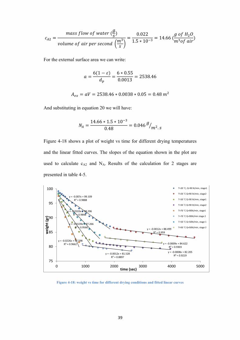
Figure 4-18 shows a plot of weight vs time for different drying temperatures
and the linear fitted curves. The slopes of the equation shown in the plot are
used to calculate cA2 and NA. Results of the calculation for 2 stages are
presented in table 4-5.
Figure 4-18: weight vs time for different drying conditions and fitted linear curves
y = -0.007x + 99.109 R² = 0.9888
y = -0.0012x + 88.499 R² = 0.959
y = -0.0139x + 97.266 R² = 0.9566
y = -0.0008x + 82.205 R² = 0.9219
y = -0.0226x + 97.598 R² = 0.9662
y = -0.0012x + 81.528 R² = 0.8897
y = -0.0103x + 98.296 R² = 0.9848
y = -0.0009x + 84.622 R² = 0.9303
75
80
85
90
95
100
0 1000 2000 3000 4000 5000
we
igh
t (g
r)
time (sec)
T=20 ˚C, Q=90 lit/min, stage1
T=20 ˚C Q=90 lit/min, stage2
T=50 ˚C Q=90 lit/min, stage1
T=50 ˚C Q=90 lit/min, stage2
T=70 ˚C Q=90lit/min, stage1
T=70 ˚C Q=90lit/min stage 2
T=50 ˚C Q=50lit/min, stage 1
T=50 ˚C Q=50lit/min, stage 2
40
Table 4-5: results of cA2 and NA for different drying conditions
dp(m) T(˚C) Q(lit/min) Re Aex(m) cA2
stage1(g/m3) NA
stage1(g/m2.s)
cA2
stage2(g/m2.s)
NA
stage2(g/m3)
1-1.7 70 90 25.28 0.48 14.66 0.046 0.8 0.0025
1-1.7 50 90 25.28 0.48 10 0.031 0.53 0.0016
1-1.7 20 90 25.28 0.48 4.26 0.013 0.8 0.0025
1-1.7 50 70 18.96 0.48 8.82 0.021 0.6 0.0014
4-4-4. Mass transfer coefficient using Stefan problem approach
The general mass transfer of species A can be expressed as:
Mass flow of species A per unit area=Mass flow of species A associated with bulk flow per unit
area-Mass flow of species A associated with molecular diffusion per unit area
Or:
��𝐴” = 𝑌𝐴(��”𝐴 + ��”𝐵) − 𝜌𝐷𝐴𝐵𝑑𝑌𝐴
𝑑𝑥 (4-13)
Where:
m”A: mass flux of species A which is mA/A (mass flow rate per unit area)
YA: mass fraction of species A
DAB: binary diffusivity of water and air (m2/s)
X: direction of mass transfer (m)
ρ: density (kg/m3)
One of the simplest approaches to calculate the rate of moisture removal in the
fluidized bed is the assumption of coal moisture to be free water contained in a
column and exposed to air flow. Taking water vapor as species A and the air
as species B we can write m”B= 0 (air is not diffusing in water vapor)
and thus the mass transfer rate equation becomes [54]:
𝑚𝐴 ” = 𝑌𝐴��”𝐴 − 𝜌𝐷𝐴𝐵𝑑𝑌𝐴
𝑑𝑥 (4-14)
Saturation mass fraction of water:
𝑌𝑤𝑎𝑡𝑒𝑟 =𝑃𝑠𝑎𝑡(𝑇)
𝑃.𝑀𝑤𝑎𝑡𝑒𝑟
𝑀 𝑚𝑖𝑥 (4-15)
41
Where Psat(T) is the saturation pressure at the drying temperature, P is the
atmosphere pressure, Mwater is the molecular weight of water and Mmix is the
interface mixture molecular weight.
Rearranging the equation and integrating will result in:
��”𝐴 =𝜌𝐷𝐴𝐵
𝐿ln (
1−𝑌∞𝑤𝑎𝑡𝑒𝑟
1−𝑌𝑤𝑎𝑡𝑒𝑟) (4-16)
To simplify the equation L=1 and we know Y∞water=0 (no moisture in the air).
Thus above equation becomes:
��”𝐴 = 𝜌𝐷𝐴𝐵ln (1
1−𝑌𝑤𝑎𝑡𝑒𝑟) (4-17)
Table 4-6: Mass flux of water leaving the bed calculated by Stefan approach
T(˚C) Psat (pa) Ywater m˙A(g/m2.s)
70 30866 0.22 7.40E-03
50 12210 0.079 2.25E-03 20 2310 0.0144 3.80E-04
Table 4-6 shows the mass flux values calculated using equation (4-17).
Comparing the flux values in tables 4-5 and 4-6, it can be seen that the value
of mass flux calculated by Stefan problem approach is significantly smaller
than that of the experiments. However, we can apply the following correction
to the mass transfer rate [55]:
��”𝐴 = [𝜌𝐷𝐴𝐵 ln (1
1−𝑌𝑤𝑎𝑡𝑒𝑟)]𝑆ℎ
2 (4-18)
Where Sh is the Sherwood number which can be calculated using Gunn
correlation [56]:
𝑆ℎ = 𝑁𝑢 = (7 − 10휀 + 5휀2). (1 + 0.7𝑅𝑒15⁄ 𝑃𝑟
13⁄ )
+ (1.33 − 2.4휀 + 1.2휀2)𝑅𝑒0.7𝑃𝑟13⁄
42
Where Re is calculated using equation (2-4) and Pr number value is 0.7 for air
[57] . The calculated Sh number is 11.88 and the corrected mass transfer rates
are presented in
Table 4-7: corrected Stefan values and experimental values for mas flux
T(˚C) Corrected mass flux
(g/m2.s) *10
3
Experimental mass
flux (g/m2.s) *10
3
70 43.95 46
50 13.36 31
20 2.28 13
As table 4-7 shows, applying the Sherwood number correction improves the
mass flux value for 70 ˚C drying significantly, but fails to result in an accurate
value for lower drying temperatures.
4-5. Calculating the activation energy of drying
To calculate the activation energy of drying process of lignite, the drying rate
k as a function of temperature can be expressed by Arrhenius equation as
follows:
𝑘 = 𝐴 𝑒𝑥𝑝(−𝐸𝑎 𝑅𝑇⁄ ) (4-18)
Where k is the drying rate, A is the pre exponential factor, Ea is the activation
energy, R is the universal gas constant (8.3143 kJ/mol) and T is the
temperature in kelvin.
Value of k is calculated based on the first 10 minutes of drying which follows
a constant rate in all temperatures for 1-1.7 mm sample and 90 lit/min gas
flow rate. Values are presented in table 4-8.
43
Table 4-8: k and ln (k) values of each temperature for 1-1.7 mm size and 90 lit/min gas flow rate
Temperature (k) Drying rate k (g/g.s) Ln(k)
343 2.92E -04 -8.14
323 1.79E -04 -8.63
293 0.89E-04 -9.33
To obtain the E and A values, the natural logarithm of drying rate versus the
reciprocal of temperature can be plot:
𝑙𝑛𝑘 = −(𝐸𝑎 𝑅)(1 𝑇⁄⁄ ) + 𝑙𝑛𝐴 (4-19)
Figure 4-9 is the plot of lnk vs. 1/T and the linear curve fitted gives the
coefficients of equation 4-18.
Figure 4-19: natural logarithmic plot of k vs. 1/T
The calculated activation energy and frequency factor are 19.68 kJ/mol and
0.283 s-1
respectively. These values are comparable with values reported in the
literature [29].
The values of k can also be taken from the diffusion model (table 4-1) which
proved to be the best fit for drying Canadian lignite. K values are presented in
table 4-9.
y = -2367x - 1.2623 R² = 0.9967
-9.6
-9.4
-9.2
-9
-8.8
-8.6
-8.4
-8.2
-8
0.0028 0.0029 0.003 0.0031 0.0032 0.0033 0.0034 0.0035
ln(K
)
1/T(1/K)
44
Table 4-9: k values taken from diffusion curve fitted to the experimental results
T (˚C) K lnk
70 0.1486 -1.90
50 0.0959 -2.34
20 0.0406 -3.20
The corresponding activation energy and pre exponential factors are 21.78
kJ/mol and 312.82 s-1
respectively.
Comparing the results with the values of 21.17 kJ/mol and 0.877 s-1
from the
literature [29], it can be concluded that the diffusion fit overpredicts the value
of frequency factor but predicts the activation energy precisely.
45
Chapter 5: CFD modeling of lignite
drying in a fluidized bed
5-1. Introduction
CFD modeling of fluidized beds is a challenging task due to the complex
nature of the problem. The hydrodynamics and phase interaction of gas-solid
flow are some of the problem complexities [49]. In this chapter, Ansys-Fluent
14.0 package has been used to simulate the drying of lignite particles in a
fluidized bed. Despite the effort to model the drying process using the
Arrhenius model (with the parameters calculated in section 4-5), only the
constant rate drying period was successfully modeled in this study.
5-2. CFD Multiphase Models
In CFD analysis, two different approaches are available to model multiphase
problems (i.e. gas-solid interaction in fluidized beds): the Euler-Lagrange
approach and the Euler-Euler approach.
5-2-1. The Euler-Lagrange approach
In this approach the fluid phase is analyzed as a continuum and Navier-Stokes
equations are solved for this phase. The dispersed phase is solved by tracing
individual particles in the fluid field. The two phases exchange transport
properties, i.e momentum etc. The main assumption made in this model is that
the dispersed phase is occupying a low volume fraction in the system. This
assumption makes this model appropriate to model spray dryers, and fuel
combustion but poorly useful in modeling liquid-liquid mixtures, fluidized
beds or generally systems with a large volume fraction of the dispersed phase
[56][49] .
46
5-2-2. The Euler-Euler approach
In this approach both the fluid and the dispersed phases are treated as
interpenetrating continua. Conservation equations are written for both phases
and each phase’s equations are related to the other using constitutive relations
obtained from empirical information of the kinetic theory [56].
Fluent provides three different Euler-Euler models:
5-2-2-1.The VOF
The VOF is a surface tracking method suitable for immiscible fluids when the
fluids interface position is to be studied. This model is applicable in problems
such as free surface fluids [56].
5-2-2-2.The mixture
This model is designed for two or more phases of fluids or particulates. The
model solves the mixture momentum equations, and using the relative
velocities, solves for the dispersed phases. Sedimentation is a good example of
application of this model [56].
5-2-2-3.The Eulerian
This is the most sophisticated model for multiphase analysis. It solves
momentum and continuity equations for each phase and couples the results
using pressure and exchange coefficients between the phases. Fluidized beds
are solved using this method [56].
In this study, Eulerian model was used to simulate the fluidized bed dryer.
5-3. Equations for Eulerian model
Conservation of mass [56]:
1
𝜌𝑟𝑞(𝜕
𝜕𝑡(𝛼𝑞𝜌𝑞) + 𝛻. (𝛼𝑞𝜌𝑞𝑣𝑞) = ∑ (𝑚𝑝𝑞
. −𝑚𝑞𝑝. ))𝑛
𝑝=1 (5-1)
47
Conservation of energy [56]:
𝜕
𝜕𝑡(𝛼𝑞𝜌𝑞ℎ𝑞) + 𝛻. (𝛼𝑝𝜌𝑝��𝑞ℎ𝑞) = −𝛼𝑞
𝜕𝑝𝑞
𝜕𝑡+ 𝜏𝑞: 𝛻��𝑞 − 𝛻. 𝑞𝑞 + 𝑆𝑞 +
∑ (𝑄𝑝𝑔 +𝑚˙𝑝𝑞ℎ𝑝𝑞 −𝑚˙𝑞𝑝ℎ𝑞𝑝𝑛𝑝=1 ) (5-2)
Fluid- Fluid Momentum balance for fluid phase q [56]:
𝜕
𝜕𝑡(𝛼𝑞𝜌𝑞𝑣𝑞) + 𝛻. (𝛼𝑞𝜌𝑞𝑣𝑞𝑣𝑞) = −𝛼𝑞𝛻𝑝 + 𝛻. 𝜏𝑞 + 𝛼𝑞𝜌𝑞𝑔 +
∑ (𝐾𝑝𝑞(��𝑝 − ��𝑞) + 𝑚𝑝𝑞. ��𝑝𝑞 −𝑚𝑞𝑝
. ��𝑞𝑝) + (𝐹𝑞 + 𝐹𝑙𝑖𝑓𝑡,𝑞𝑛𝑝=1 + 𝐹𝑣𝑚,𝑞) (5-3)
Where 𝜏q is the stress-strain tensor [56]:
𝜏𝑞 = 𝛼𝑞µ𝑞(𝛻𝑣𝑞 + 𝛻𝑣𝑞𝑇) + 𝛼𝑞 (𝜆𝑞 −
2
3µ𝑞)𝛻. 𝑣𝑞𝐼 (5-4)
And Kpq is the interphase momentum exchange coefficient.
For solid- fluid momentum exchange an equation similar to (5-3) is used with
Kls, momentum exchange coefficient between fluid l and solid s. Fluent uses
different models to define this momentum exchange coefficient. Some of the
available models include Syamlal-Obrein, Gidaspow, Wen-Yu etc. The best
model to predict the solid-gas exchange coefficient for fluidized beds is
proved to be Syamlal-Obrein.
In this study, Syamlal-Obrein drag was used to evaluate the fluidization
behavior.
5-4. Syamlal-O’brein Drag model
The general form for the solid-gas exchange coefficient is[56]:
𝐾𝑙𝑠 =𝑎𝑠𝜌𝑠𝑓
𝜏𝑠 (5-5)
Where 𝜏s is the “particulate relaxation time” in the form of:
𝜏𝑠 =𝜌𝑠𝑑𝑝
2
18µ𝑙 (5-6)
48
and f includes a drag function CD based on relative Reynolds number.
In the model suggested by Syamlal and Obrein (1987) CD is defined as:
𝐶𝐷 = (0.63 +4.8
√𝑅𝑒𝑠𝑣𝑟,𝑠
)
2
(5-7)
Where Res is defined as:
𝑅𝑒𝑠 =𝜌𝑙𝑑𝑝(|��𝑠−��𝑔|)
µ𝑙 (5-8)
And vr,s is the terminal velocity ratio:
𝑣𝑟𝑠 = 0.5(𝐴 − 0.06𝑅𝑒𝑠 +√(0.06𝑅𝑒𝑠)2 + 0.12𝑅𝑒𝑠(2𝐵 − 𝐴) + 𝐴
2 ) [58] (5-9)
With: 𝐴 = 𝛼𝑔4.14 (5-10) and
𝐵 = 𝑝𝛼𝑔1.28 (5-11) for αg ≤0.85
And 𝐵 = 𝛼𝑔𝑞 (5-12) for αg ˃0.85
The values of p and q are 0.8 and 2.56 respectively. Then the solid-fluid
exchange coefficient becomes [58]:
𝐾𝑠𝑙 =3𝛼𝑠𝛼𝑔𝜌𝑔
4𝑣𝑟𝑠2 𝑑𝑠
𝐶𝐷 (𝑅𝑒𝑠
𝑣𝑟𝑠) |��𝑠 − ��𝑔| (5-13)
5-5. Boundary conditions
Inlet:
- Gas velocity = 0.4 m/s
- Gas temperature = 293K, 343 K
- Mass fraction of H2O= 0
Outlet:
- outflow
Wall:
49
- Momentum: No slip
- Species: Zero diffusive flux
5-6. Initial conditions
- Solid volume fraction= 0.55
- Solid temperature= 300 K
- Solid velocity= 0
Figure 5-1: Bed mesh and Boundaries
This model was applied to the Fluent along with the input data and settings
presented in tables 5-1 and 5-2.
50
Table 5-2: Solver Spatial discretization
Parameter Spatial Discretization
Gradient Least square cell based
Momentum Quick
Volume fraction Modified HRIC
Energy Quick
Gas species Quick
Solid species Quick
In table 5-1, the value for mass transfer rate is the experimental values for 70
˚C and 20 ˚C tests. The model predicts minimum fluidization velocity of 30.66
m/s for the bed which is 25% less than 0.4 m/s. This model was used to model
the bed momentum exchange and the results for solid volume fraction are
shown in figure 5-2.
Parameter Value
Particle diameter 1.3e-03 m
Particle density 1400 kg/m3
Solid volume fraction 0.55
Packing limit 0.58
Gas velocity 0.4 m/s
Gas temperature 20˚C and 70 ˚C
Solid initial temperature 20 ˚C (293 K)
Mass transfer rate 0.06 and 0.21 kg/m3.s
Time steps 10e-04 s
No. of iteration per time step 70
Operating pressure 101325 pa
Number of mesh cells 5544
Min/Max cell size 2.35e-03/2.493-03 m2
Mesh aspect ratio 1.45
Smallest Residual 10e-04
Table 5-1: Input parameters for Fluent
51
Figure 5-2: solid volume fraction in the first 1.13 sec using Syamlal-Obrein Drag model
As you can see in figure 5-2, the solid phase leaves the bed in the first 1.13 sec
entirely, proving that the drag model does not predict the bed behavior
correctly.
5-4. Tuned Syamlal-Obrein model
To make Syamlal-Obrein drag model predict the bed momentum exchange
correctly, p and q coefficients need to be tuned to predict the appropriate
velocity. To do so, we need to know the value for the particle terminal velocity
ratio. We can write:
𝑣𝑟,𝑠 =𝑅𝑒𝑠
𝐴𝑟∗ (5-14)
Where Res can be calculated from equation (5-8) and Ar* is a dimensionless
function of the Archimedes number as:
𝐴𝑟∗ =
(
√4.82+2.52(√
4𝐴𝑟
3)−4.8
1.26
)
2
(5-15)
52
Substituting the value for vr,s as 0.164, ( which can be compared to 0.277, the
value calculated by default p and q numbers) in equation 5-9 and iterating for
A and B (using a programming code) the calculated values of coefficients p
and q for this case were 0.491 and 5.66223 respectively. These values were
used in a UDF file which is compiled by fluent to evaluate the solid-gas
momentum exchange coefficient using Syamlal-Obrein model. Figure 5-3
shows the solid volume fraction during the first 5.22 sec of the modeling using
the tuned drag model. It can be noticed that the bed reached a stable condition
in 0.5 sec.
Figure 5-3: solid volume fraction calculated by tuned Syamlal-Obrein drag model
53
Figure 5-4: mass flux vs. time of H2O at the outlet for T=20 ˚C and 70 ˚C
Figure 5-4 shows a plot of mass flux of water versus time for 2 different
drying temperatures. The plot shows that the water flux for 70 ˚C is almost 5
times higher than that of 20 ˚C. Comparing the software results with that of
the experiment (table 4-5), it can be seen that the software has predicted the
moisture removal successfully.
0
0.005
0.01
0.015
0.02
0.025
0.03
0.035
0.04
0.045
0.05
0 1 2 3 4 5 6 7
mas
s fl
ux
(g/m
2 .s)
time (sec)
70 ˚C, simulation
20 ˚C, simulation
T= 70 ˚C, experiment
T=20 ˚C, experiment
54
Chapter 6: Spontaneous combustion of
lignite To evaluate the spontaneous combustion risk of dried lignite, a series of
experiments in a TGA-DSC were carried out. Around 10 mg of dried samples
were heated up in the TGA-DSC in air atmosphere. Samples were heated up
from room to 400 °C at different heating rates of 0.4 °C/min, 1 °C/min and 2
°C/min. Sample was then kept in an isotherm condition for 1 hour before
cooling down to room temperature. The weight loss and heat flow of the
samples were recorded by the instrument.
Figure 6-1: TGA-DSC signal of 2 C/min test
Figure 6-1 is the plot of weight, weight derivative and heat flow versus
temperature for the 1 °C/min run. As you can see in the plot, the peaks
indicate a reaction in the sample at a certain temperature. In the heat flow
curve, the highest peak corresponds to the combustion of coal sample. In this
55
study, the onset temperature of the curves, were the sample starts releasing
heat is taken as the temperature of spontaneous reaction.
Figure 6-2: weight loss derivative of dried samples at 0.4, 1, 2 ˚C/min
Figure 6-2 is a plot of the weight derivative vs. temperature for the three runs.
As expected, in higher heating rates, the reaction happens in a higher
temperature which is due to a thermal lag.
To study the spontaneous combustion kinetics, the Semenov theory was used.
According to this theory, the difference between the heat production and heat
loss of the system defines the risk of an explosion in the system. Writing the
energy balance in this way we can have [47]:
𝐶𝑝𝑀0𝑑𝑇
𝑑𝑡= 𝛥𝐻𝑀0 𝐴𝑒𝑥𝑝(−
𝐸𝑎
𝑅𝑇) − 𝑈𝑆(𝑇 − 𝑇0) (6-1)
Where:
Cp is the heat capacity of the system
M0 is the initial mass of the reactant
ΔH is the heat of combustion per unit mass of reactant
56
A is the pre exponential factor
Ea is the activation energy
U is the overall heat transfer rate
S is the total surface area
T0 is the ambient temperature
At the critical temperature both dT/dt and d(dT/dt)/dT are equal to zero and
the ambient temperature must be equal to the self-heating oxidation (SHOT)
[47]. So we will have:
𝛥𝐻𝐴𝑀0 exp (−𝐸𝑎
𝑅𝑇𝑐𝑟) = 𝑈𝑆(𝑇𝑐𝑟 − 𝑇0) (6-2)
And
𝛥𝐻𝐴𝑀0𝐸𝑎
𝑅𝑇𝑐𝑟2 exp (−
𝐸𝑎
𝑅𝑇𝑐𝑟) = 𝑈𝑆 (6-3)
Dividing the two equations and rearranging for T0 will give:
𝑇0 = 𝑆𝐻𝑂𝑇 = 𝑇𝑐𝑟 −𝑅𝑇𝑐𝑟
2
𝐸𝑎 (6-4)
To be able to calculate SHOT, activation energy, heat of combustion and pre-
exponential factor can be calculated using the TGA-DSC data.
The same calculations that were carried out for activation energy of drying can
be used to calculate spontaneous combustion activation energy. This included
plotting LnK vs. 1/T for the reaction and taking a linear regression. In here the
reaction rate and T data of different heating rate runs were used at 50 % of
conversion.
Table 6-1: kinetic values of combustion in different heating rates
T (˚C)
Heating rate
(˚C/min)
Reaction rate
(mg/min) ln Rate
259.18 0.4 0.034 -3.372
315.23 1 0.069 -2.662
333.06 2 0.18 -1.682
57
Figure 6-3: ln rate vs. 1/T at conversion of 0.5
As figure 6-3 shows, linear regression of the data gives the activation energy
of 131.29 kj/mol and pre-exponential factor of 3.77e10 1/s.
Table 6-2: thermodynamic and kinetic of dried coal
Heating
rate
(°C/min)
ΔH
(J/kg) M0 (mg) S (mm2) T onset(°C) Tcr (°C) SHOT(°C)
0.4 8785 13.47 580.347 148 154.5 142.9265
1 14458 10.5 452.386 160 164 151.9064
2 15243 12.96 558.374 178.3 176 163.2331
Table 6-2 presents the SHOT calculated values. As you can see SHOT values
are good estimation of the onset temperature at which coal particles start
releasing heat, leading to the spontaneous combustion.
y = -15791x + 24.353 R² = 0.9705
-4
-3.5
-3
-2.5
-2
-1.5
-1
-0.5
00.00164 0.00166 0.00168 0.0017 0.00172 0.00174 0.00176 0.00178
58
Chapter 7: Summary and Conclusion
7-1. Summary
Low temperature coal drying was studied in a pilot scale fluidized bed
dryer. Lignite samples in the size range of 1-2.8 mm, with initial moisture
of 21% were dried in the temperature range of 20 ˚C to 70 ˚C.
Samples density was measured to be 1400 kg/m3 using the water
displacement method.
Fluidization regime was not effectively achieved in the bed because lignite
samples, belonging to the group D of Geldard classification (known to be
difficult to be fluidized) have high density, large particle size and low
sphericity.
Temperature showed a great effect on the drying rate in the constant rate
period while being poorly effective in the falling rate period.
Decreasing gas flow rate to 30 % below the theoretical minimum
fluidization velocity showed satisfactory drying results.
Modeling the lignite drying as a packed bed of free water exposed to low
air stream under predicted the drying rate. Because despite the fact that
particles are not fluidized in the bed, the upward air velocity through
particles provides a high mass and heat transfer.
Increasing particle size decreased the mass transfer rate and coefficient due
to thermal lag and a smaller surface area contact.
Drying data was curve fitted using mathematical models available in the
literature and the logarithmic model best fitted the drying of lignite.
59
Diffusion coefficient of lignite drying was calculated using the experiment
data and was in a good degree of agreement with the value reported in the
literature.
Fluidized bed dryer was modeled using CFD analysis. Default Syamlal-
Obrein drag model failed to predict the velocity profile correctly but
tuning the model’s coefficients improved the accuracy of the model
compared to the experiment. Constant rate drying was successfully
modeled in Fluent using a single mass transfer mechanism.
Spontaneous combustion kinetic of dried lignite was studied. The onset
temperature of the mass derivative curve, corresponding to the
spontaneous combustion was measured experimentally and using the
Semenov theory the temperature was calculated and showed good
agreement with the measured value.
7-2. Conclusion
Based on the data analysis, when drying lignite coal particles in a packed
bed dryer, it is more efficient to use higher drying temperatures in the
constant drying period and lower drying temperatures in the falling rate
period.
If spouted bed is not desired to be used for lignite drying, packed bed of
lignite particles can be dried efficiently without increasing air velocity to
the theoretical minimum fluidization.
The self-heating oxidation temperature of lignite can be calculated using
the Semenov theory. This temperature can be calculated and used to
predict the reaction temperature.
60
Reference
[1] “world coal association” http://www.worldcoal.org. [Accessed: 20-Oct-
2014].
[2] “Energy industry today” http://www.energy.einnews.com. [Accessed:
22-Sep-2014].
[3] J. Yu, A. Tahmasebi, Y. Han, F. Yin, and X. Li, “A review on water in
low rank coals: The existence, interaction with coal structure and
effects on coal utilization,” Fuel Process. Technol., vol. 106, pp. 9–20,
Feb. 2013.
[4] coal association of Canada, “careers in coal.”
http://www.careersincoal.ca/mine-map/.
[5] “Alberta energy” http://www.energy.alberta.ca
[6] R. S. D.J. Allardice, L.M. Clemow, G. Favas, W.R. Jackson, M.
Marshall, “The characterisation of different forms of water in low rank
coals and some hydrothermally dried products,” Fuel, vol. 82, pp. 661–
667, 2003.
[7] J. Choung, C. Mak, Z. Xu, “Fine coal beneficiation using an air dense
medium,” coal Prep., pp. 1–15, 2006.
[8] R. G. Domazetis, P. Barilla, B.D. James, “Treatments of low rank coals
for improved power generation and reduction in greenhouse gas
emissions,” Fuel Process. Technol., vol. 89, pp. 68–76, 2008.
[9] P. C. Dave, “Dry Cleaning of Coal by a Laboratory Continuous Air
Dense Medium Fluidized Bed Separator", MSc thesis, Mining
Engineering, University of Alberta, 2012.
[10] H. Katalambula and R. Gupta, “Low-Grade Coals : A Review of Some
Prospective Upgrading Technologies,” Energy and Fuels, vol 23, pp.
3392–3405, 2009.
[11] C.E. Salmas, A.H. Tsetsekou, K.S. Hatzilyberis, G.P.
Androutsopoulos, “Evolution lignite mesopore structure during drying.
effect of temperature and heating time,” Dry. Technol., vol. 19, pp. 35–
64, 2001.
[12] N. Sarunac, E. K. Levy, M. Ness, C. W. Bullinger, J. P. Mathews, and
P. M. Halleck, “A Novel Fluidized Bed Drying and Density
Segregation Process for Upgrading Low-Rank Coals,” Int. J. Coal
Prep. Util, vol. 29, no. 6, pp. 317–332, Dec. 2009.
61
[13] I.J. Lynch, D.S. Webster, “Effect of thermal treatment on the
interaction of brown coal and water: a nuclear magnetic resonance
study,” Fuel, vol. 61, pp. 271–275, 1982.
[14] S.C. Mraw, D.F. Naas-O'Rourke, “Water in coal pores: low-
temperature heat capacity behavior of the moisture in Wyodak coal,”
Science, vol. 205, pp. 901–902, 1979.
[15] D.J. Allardice, D.G. Evans, "Analytical Methods for Coal and Coal
Products". New York: Academic Press, 1978.
[16] W. G. Willson, D. Walsh, and W. (Bill)Irwinc, “Overview of Low-
Rank Coal (LRC) Drying,” Coal Prep., vol. 18, no. 1–2, pp. 1–15, Jan.
1997.
[17] M. Karthikeyan, W. Zhonghua, and A. S. Mujumdar, “Low-Rank Coal
Drying Technologies—Current Status and New Developments,” Dry.
Technol., vol. 27, no. 3, pp. 403–415, Feb. 2009.
[18] P. K. Chen, Z., Wu, W., Agarwal, “Steam-drying of coal. Part 1.
Modeling the behavior of a single particle,” Fuel, vol. 79, pp. 961–973,
2000.
[19] “ http://www.wikipedia.com" [Accessed: 22-Oct-2014].
[20] Bergins, Christian, “Science and Technology of the Mechanical /
Thermal Dewatering,” 2005.
[21] GEA group, “GEA Process Engineering Inc.” http://www.niroinc.com.
[Accessed: 22-Oct-2014].
[22] C. Mak, “Fine coal cleaning using an air dense medium fluidized bed,”
Alberta, 2007.
[23] M. Rhodes, “Introduction to particle technology,” 2nd ed., M. Rhodes,
Ed. pp. 193–235.
[24] P. Zhao, Y. Zhao, Z. Luo, Z. Chen, C. Duan, and S. Song, “Effect of
operating conditions on drying of Chinese lignite in a vibration
fluidized bed,” Fuel Process. Technol., vol. 128, pp. 257–264, Dec.
2014.
[25] G. Chase, “Solids notes,” 2004, pp. 5–1 to 5–11.
[26] D. Geldart, “Types of Gas Fhidization,” Powder Technol., vol. 7, pp.
285–292, 1973.
[27] W.-C. Wang, “Laboratory investigation of drying process of Illinois
coals,” Powder Technol., vol. 225, pp. 72–85, Jul. 2012.
62
[28] K. S. Vorres, “Effect of Temperature, Sample Size, and Gas Flow Rate
on Drying on Beulah-Zap Lignite and Wyodak Subbituminous Coal,”
Energy & Fuels, vol. 8, no. 2, pp. 320–323, Mar. 1994.
[29] A. Tahmasebi, J. Yu, Y. Han, H. Zhao, and S. Bhattacharya,
“Thermogravimetric study and modeling for the drying of a Chinese
lignite,” ASIA-PACIFIC J. Chem. Eng., vol. 8, no. February, pp. 793–
803, 2013.
[30] H. Wang, “Kinetic Analysis of Dehydration of a Bituminous Coal
Using the TGA Technique,” no. 10, pp. 3070–3075, 2007.
[31] C.Srinivasakannan and N.Balasubramanian, “A simplified approach to
the drying of solids in a batch fluidized bed,” Brazilian J. Chem. Eng.,
vol. 19, pp. 293–298, 2002.
[32] A. N. Chandran, S. Subba Rao, and Y. B. G. Varma, “Fluidized Bed
Drying of Solids,” AIChE J., vol. 36, pp. 29–38, 1990.
[33] E. K. Levy, H. S. Caram, Z. Yao, Z. Wei, and N. Sarunac, “Kinetics of
coal drying in bubbling fluidized beds” Proceedings Fifth World
Congress on Particle Technology, Orlando, Florida. 2006.
[34] W. Ciesielczyk and J. Iwanowski, “Analysis of Fluidized Bed Drying
Kinetics on the Basis of Interphase Mass Transfer Coefficient,” Dry.
Technol., vol. 24, no. 9, pp. 1153–1157, Sep. 2006.
[35] S. Syahrul, I. Dincer, and F. Hamdullahpur, “Thermodynamic modeling
of fluidized bed drying of moist particles,” Int. J. Therm. Sci., vol. 42,
no. 7, pp. 691–701, Jul. 2003.
[36] J. Cai and R. Liu, “Kinetic Analysis of Solid-State Reactions: A
General Empirical Kinetic Model,” Ind. Eng. Chem. Res., vol. 48, no. 6,
pp. 3249–3253, Mar. 2009.
[37] T.-J. Kang, H. Namkung, L.-H. Xu, S. Lee, S. Kim, H.-B. Kwon, and
H.-T. Kim, “The drying kinetics of Indonesian low rank coal (IBC)
using a lab scale fixed-bed reactor and thermobalance to apply catalytic
gasification process,” Renew. Energy, vol. 54, pp. 138–143, Jun. 2013.
[38] J. Burgschweiger, H. Groenewold, C. Hirschmann, and E. Tsotsas,
“From hygroscopic single particle to batch fluidized bed drying
kinetics,” Can. J. Chem. Eng., vol. 77, no. 2, pp. 333–341, Apr. 1999.
[39] E. Mirzaee, S. Rafiee, and A. Keyhani, “Determining of moisture
diffusivity and activation energy in drying of apricots,” vol. 2009, no.
Yadollahinia 2006, pp. 114–120, 2009.
63
[40] R. G. Szafran and A. Kmiec, “CFD Modeling of Heat and Mass
Transfer in a Spouted Bed Dryer,” Ind. Eng. Chem. Res., vol. 43, no. 4,
pp. 1113–1124, Feb. 2004.
[41] S. Azizi, S. H. Hosseini, M. Moraveji, and G. Ahmadi, “CFD modeling
of a spouted bed with a porous draft tube,” Particuology, vol. 8, no. 5,
pp. 415–424, Oct. 2010.
[42] T. J. Jamaleddine and M. B. Ray, “The Drying of Sludge in a Cyclone
Dryer Using Computational Fluid Dynamics,” Dry. Technol., vol. 29,
no. 12, pp. 1365–1377, Sep. 2011.
[43] W. Sujanti and D. Zhang, “A laboratory study of spontaneous
combustion of coal: the influence of inorganic matter and reactor size,”
Fuel, vol. 78, no. 5, pp. 549–556, Apr. 1999.
[44] Z. Mao, H. Zhu, X. Zhao, J. Sun, and Q. Wang, “Experimental Study
on Characteristic Parameters of Coal Spontaneous Combustion,”
Procedia Eng., vol. 62, pp. 1081–1086, 2013.
[45] Y. Yang, Z. Li, S. Hou, F. Gu, S. Gao, and Y. Tang, “The shortest
period of coal spontaneous combustion on the basis of oxidative heat
release intensity,” Int. J. Min. Sci. Technol., vol. 24, no. 1, pp. 99–103,
Jan. 2014.
[46] G. Qi, D. Wang, Y. Chen, H. Xin, X. Qi, and X. Zhong, “The
application of kinetics based simulation method in thermal risk
prediction of coal,” J. Loss Prev. Process Ind., vol. 29, pp. 22–29, May
2014.
[47] X. Zhao, H. Xiao, Q. Wang, P. Ping, and J. Sun, “Study on spontaneous
combustion risk of cotton using a micro-calorimeter technique,” Ind.
Crops Prod., vol. 50, pp. 383–390, Oct. 2013.
[48] “ASTM B311-13, Standard Test Method for Density of Powder
Metallurgy (PM) Materials Containing Less Than Two Percent
Porosity, ASTM International, West Conshohocken, PA, 2013,
www.astm.org.”
[49] E. Azimi, “Simulation and performance characterization of air dense
medium fluidized bed for coal beneficiation", PhD thesis, University of
Alberta, 2014
[50] M. a. Hossain and B. K. Bala, “Thin-Layer Drying Characteristics for
Green Chilli,” Dry. Technol., vol. 20, no. 2, pp. 489–505, Feb. 2002.
[51] www.chemistry.about.com.
[52] C. J. Geankoplis, "Transport Processes and Separation Process
Principles", Fourth ed. 2003.
64
[53] J. Crank," The mathematics of diffusion", 2nd
edition. Oxford university
press, 1975.
[54] S. R. Turns, "An introduction to Combustion", 3rd
edition.
McGraw.Hill, 2012, pp. 88–93.
[55] Petr A. Nikrityuk, B. Meyer, (Eds). "Gasification Processes Modeling
and Simulation". Wiley-VCH, p. 127.
[56] "ANSYS-FLUENT® Theory Guide, Release 14.0, 2013.” .
[57] www.engineeringtoolbox.com. [Accessed: 15-Jun-2014].
[58] P. Lela, N. Ramesh, M. Raajenthiren, “A review of some existing drag
models describing the interaction between the solid- gaseous phase in
CFB,” Int. J. Eng. Sci. Technol., vol. 2, no. 5, pp. 1047–1051, 2010.
65
Appendix A: Calculating minimum fluidization
ρp =1400 kg/m3
ρg =1.004 kg/m3
µg =0.00001983
dp =13 mm
using eq 2-3 we can write
𝐴𝑟 =𝜌𝑔(𝜌𝑝−𝜌𝑔)𝑔 𝑑𝑝
3
µ𝑔2 =
1.004(1400−1.004)∗9.81∗(0.0013)3
(𝑜.𝑜𝑜𝑜𝑜1983)2= 70659.2
Using eq 2-5:
𝑅𝑒𝑚𝑓 = 33.7[(1 + 3.59 ∗ 10−5𝐴𝑟)0.5 − 1] = 29.6
Using eq 2-4:
𝑢𝑚𝑓 =𝑅𝑒∗µ𝑔
𝜌𝑔𝑑𝑝=31.6∗0.00001983
1.004∗0.00135= 0.46 𝑚/𝑠
Bed diameter =7 cm → Bed cross section area A= 38 cm2
Air flow rate Q = umf . A=1.
5e-03 m3/s = 90 lit/min