LP-based solution methods for single-machine schedulingproblemsCitation for published version (APA):Akker, van den, J. M. (1994). LP-based solution methods for single-machine scheduling problems. TechnischeUniversiteit Eindhoven. https://doi.org/10.6100/IR428838

DOI:10.6100/IR428838

Document status and date:Published: 01/01/1994

Document Version:Publisher’s PDF, also known as Version of Record (includes final page, issue and volume numbers)

Please check the document version of this publication:

• A submitted manuscript is the version of the article upon submission and before peer-review. There can beimportant differences between the submitted version and the official published version of record. Peopleinterested in the research are advised to contact the author for the final version of the publication, or visit theDOI to the publisher's website.• The final author version and the galley proof are versions of the publication after peer review.• The final published version features the final layout of the paper including the volume, issue and pagenumbers.Link to publication

General rightsCopyright and moral rights for the publications made accessible in the public portal are retained by the authors and/or other copyright ownersand it is a condition of accessing publications that users recognise and abide by the legal requirements associated with these rights.

• Users may download and print one copy of any publication from the public portal for the purpose of private study or research. • You may not further distribute the material or use it for any profit-making activity or commercial gain • You may freely distribute the URL identifying the publication in the public portal.

If the publication is distributed under the terms of Article 25fa of the Dutch Copyright Act, indicated by the “Taverne” license above, pleasefollow below link for the End User Agreement:www.tue.nl/taverne

Take down policyIf you believe that this document breaches copyright please contact us at:openaccess@tue.nlproviding details and we will investigate your claim.

Download date: 25. Mar. 2022

LP-based solution methods

for

single-machine scheduling problems

,• - - - -·' , ' , '

' '

•

• •

Marjan van den Akker

LP-based solution methods for

single-machine scheduling problems

LP-based solution methods for

single-machine scheduling problems

PROEFSCHRIFT

ter verkrijging van de graad van doctor aan de Technische Universiteit Eindhoven, op gezag van de Rector Magnificus, prof.dr. J.H. van Lint, voor een commissie aangewezen door het College van Dekanen in het openbaar te verdedigen op

woensdag 21 december 1994 om 16.00 uur

door

JANNA MAGRIETJE VAN DEN AKKER

geboren te Gouda

Dit proefschrift is goedgekeurd door de promotoren

prof.dr. J .K. Lenstra en prof.dr. M.W.P. Savelsbergh

Copromotor: dr.ir. C.A.J. Hurkens

Ter herinnering aan mijn vader, voor mijn moeder en mijn broer.

Acknowledgements

The process of writing this thesis has been completed successfully thanks to the help of a nurnber of people.

In the first place, 1 want to thank my supervisors Jan Karel Lenstra and Martin Savelsbergh. Jan Karel was an excellent manager and gave many valuable com­ments on rny manuscripts. Martin helped to ask the right question at the right moment. I want to thank him for the many stimulating discussions we had and for his help in writing this thesis.

I feel much indebted to Stan van Hoesel. While having coffee, we generated many good ideas concerning valid inequafüies. I am grateful to Cor Hurkens, especially for a very useful remark concerning the characterization and for all his help with the computer. I thank my roommate Cleola van Eyl for always being there to solve practical problems and Ann Vandevelde for helping me to draw pictures with the computer. Furthermore, I want to thank Frits Spieksma for sending me unpublished notes and Bob Bixby for solving sorne large test instances.

1 want to thank Jack Kooien for bis friendship and for the many humorous discus­sions.

Finally, 1 want to thank Han for being involved in so many ways.

Marjan van den Akker

1

Contents

1 Introduction 5 1.1 Scheduling . . ~ . . . . . . . 5 1.2 Complexity ......... 7 1.3 Integer linear programming . 7 1.4 Polyhedral combinatorics . 8 1.5 Branch-and-cut ... 11 1.6 Column generation 12 1.7 Outline of the thesis . 14

2 Mixed-integer programming formulations for single-machine sche­duling problems 17 2.1 Introduction . . . . . . . . . . . . . . . . . . . . . . . . . . . . . . 17 2.2 Formulations based on completion times . . . . . . . . . . . . . . . 17 2.3 Formulations based on start times and sequence determining variables 20 2.4 Time-indexed formulations . . . . . . . . . . . . . . . . . . . . . . 24 2.5 A formulation based on positional start times and position deter-

mining variables . . . . . . . . . . . . . . . . . . . . . . . . . . . . 26

3 Facets and characterizations 3.1 Introduction .... 3.2 Special cases . . . .

3.2.1 Minimîzing Ci 3.2.2 Minimizing wiCi

3.3 Basic properties of the polyhedral structure 3.4 Facet inducing inequalities wit.h right-hand side 1 . 3.5 Facet inducing inequalities with right-hand sîde 2 .

3.5.1 Case (Ia) 3.5.2 Case (Ib) 3.5.3 Case (2) .

3.6 Related research .

2

29 29 30 30 32 37 39 42 46 53 59 67

4 Separation and computation 4.1 Introduction . . . . . . . . . 4.2 Separation . . . . . . . . . . . . . . . . . . . . . . . . . . . . . . .

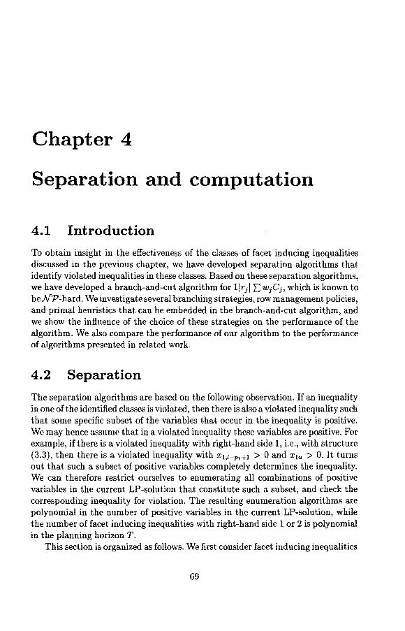
4.2.1 A separation algorithm for facet inducing inequalities with right-hand side 1 ...................... .

4.2.2 Separation algorithms for facet inducing inequalities with right-hand side 2 .......... .

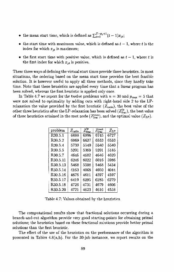
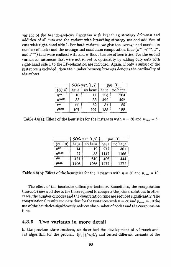
4.3 A branch-and-cut algorithm for l lr11 :L wiCi 4.3.1 Quality of the lower bounds 4.3.2 Branching strategies 4.3.3 Row management . . . . . . 4.3.4 Prima! heuristics ..... . 4.3.5 Two variants in more detail .

4.4 Related work . . . . . . . . . . . .

5 Column generation 5.1 Introduction .............. . 5.2 Solving the LP-relaxation . . . . . .. . 5.3 Combining row and column generation 5.4 Branching . . . . 5.5 Key formulations

Bibliography

Samenvatting

Curriculum vitae

3

69 69 69

70

71 77 78 80 84 88 90 91

95 95 96

103 109 110

117

123

129

Chapter 1

Introduction

1.1 Sched uling

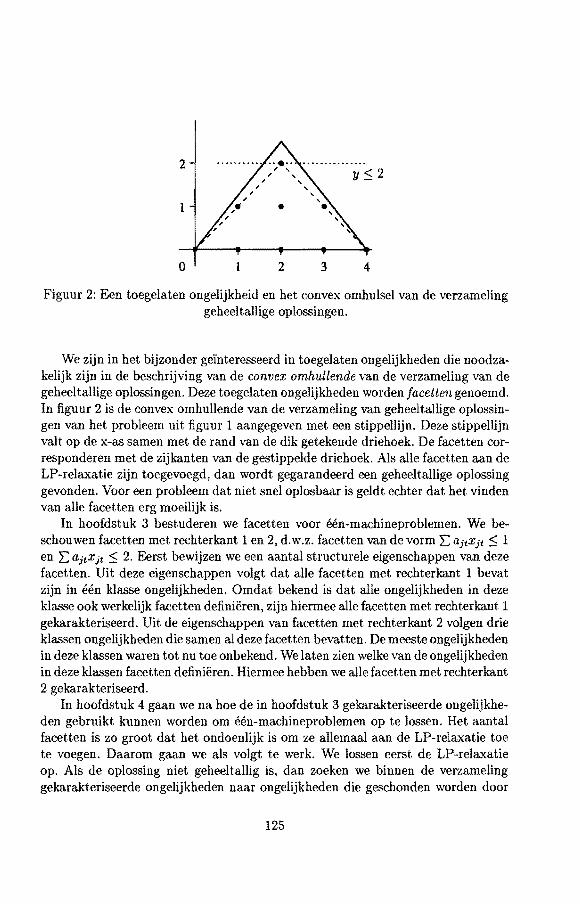
Imagine one of the following situations. In a factory products have to be manufac­tured by different machines, where each machine can handle at most one product at a time. Tasks assigned toa multiprogrammed computer system compete for pro­cessing on a timesharing basis. In a school lessons have to be assigned to teachers such that each lesson is given by a teacher capable of teaching that lesson. Planes requesting to use an airport runway are assigned places in a queue. In each of these situations a number of tasks has to be processed using one or more resources with limited capacity and availability, such as machines, tools, or employees. Usually, one wants to find an allocation of the tasks to the resources such that the workload of any resource does not exceed its capacity and the costs are minimal. Many of such problems can be modeled as scheduling problems, which are problems that concern the allocation of jobs to machinesoflimited capacity and availability. For instance, in the school example the jobs are the lessons and the machines are the teachers. Motivated and stimulated by the practical relevance, scheduling has become an important area of operations research.

We consider nonpreemptive single-machine scheduling problems. The usual set­ting for such a problem is as follows. A set of n jobs has to be scheduled on a single machine. Each job j (j = 1, ... , n) must be processed without interruption during a period of length Pi· The machine can handle no more than one job at a time and is continuously available from time zero onwards. We are asked to find an optima} feasible schedule, that is, a set of complet.ion times such that the capacity and avail­ability constraints are met and a given objectivdunction is minimized. It is possible that precedence relations have been specified, i.e., for each job j (j 1, ... , n) there is a set of jobs that have to precede job j and a set of jobs that have to succeed job j in any feasible schedule. It. is further possible that each job is only available for processing during a prespecified period of time; job j may have a release date rj, at which it becomes available, and a deadline dj, by which it must be completed. In addition, it may have a positive weight w3, which expresses its importance with

5

respect to the other jobs, and a due date dj, which indicates the time by which it ideally should be completed. A due date differs from a deadline in the sense that a deadline is 'hard', whereas a due date may be exceeded at a certain cost. The weights and due dates are typically used to define the objective function. Some well-known objective functions are the weighted sum of the completion times and the weighted sum of the tardinesses; the tardiness Tj of job j is equal to the amount of time by which it exceeds its due date, if it is completed after that time, and 0 otherwise, i.e., T1 = max{O, Ci d1 }, where C1 denotes the completion time of job j. In the sequel, scheduling problems will be specified in terms of a three-field classification al.Bh', where

• a describes the machine environment: fora single-machine scheduling prob­lem we have a = 1;

• ,8 describes the job characteristics: pree indicates that precedence relations have been specified, sepa that the precedence relations are series-parallel, pj = p that all processing times are equal top, and ri and dj that release dates and deadlines have been specified, respectively;

• 7 represents the objective function.

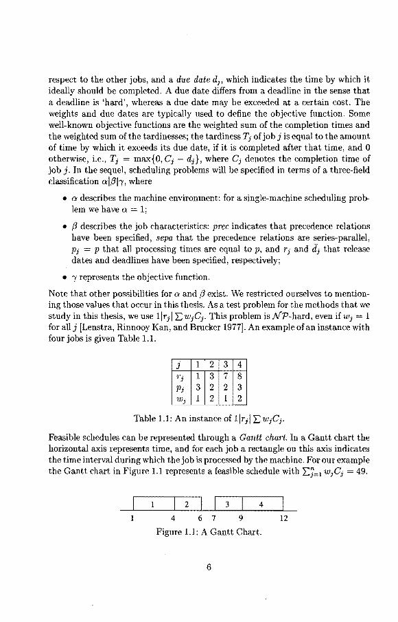
Note that other possibilities fora: and ,8 exist. We restricted ourselves to mention­ing those values that occur in this thesis. As a test problem for the methods that we study in this thesis, we use 1lrj1 L: wjCj. This problem is NP-hard, even if Wj = 1 for allj [Lenstra, Rinnooy Kan, and Brucker 1977]. An example of an instance with four jobs is given Table 1.1.

j 1 2 3 4 Tj 1 3 7 8 Pj 3 2 2 3 Wj 1 2 1 2

Table 1.1: An instance of llrJI L: WJC;.

Feasible schedules can be represented through a Gantt chart. In a Gantt chart the horizontal axis represents time, and for each job a rectangle on this axis indicates the time interval during which the job is processed by the machine. For our example the Gantt chart in Figure 1.1 represents a feasible schedule with L:j=1 wjCj = 49.

4 6 7 9 12

Figure 1.1: A Gantt Chart.

6

1.2 Complexity The scheduling problems that are considered in this thesis fall in the area of com­binatorial optimization. Combinatorial optimization involves problems in which we have to choose an optimal solution from a fini te number of potential solutions. We consider a solution to be optimal if it has minimum objective value. Many combinatorial optimization problems, including some well-known single-machine scheduling problems, are N'P-hard. This means that no algorithm is known that solves each instance of the problem to optimality in time polynomial with respect to the size of the instance, and that it is considered very unlikely that such an algorithm exists. Hence, if we wish to solve the problem to optimality, then we should allow for algorithms that may take exponential time. An example of such an approach is branch-and-bound, which implicitly enumerates the set of all feasible solutions. Branch-and-bound proceeds by splitting the set of feasible solutions into subsets (this is the branching part). For each generated subset a lower bound on the value of the best solution is computed. If this lower bound exceeds the value of a known feasible solution, then we can skip the subset without further inspection (this is the bounding part). In order to be able to apply branch-and-bound effec­tively, it is of the utmost importance to find good lower bounds that can be easily computed.

1.3 Integer linear programming

Combinatorial optimization problems can be formulated as integer linear pro­grams, which implies that integer linear programming is N'P-hard. If we relax the integrality conditions, then we obtain a linear programming problem, which is called the LP-relaxation; the optimal valne of this problem is a lower bound on the optimal value of the original problem. Since there are algorithms that solve any instance of linear programming to optimality in polynomial time (Khachiyan [1979], Karmarkar [1984]), this lower bound can be computed efficiently. Solving LP-relaxations can hence be used as a lower bounding strategy in a branch-and­bound algorithm.

For nonpreemptive single-machine scheduling problems different mixed-integer programming formulations have been proposed; we give a survey in the next chap­ter. In this thesis, we consider a time-inde.Ted formulation that bas been studied before by Sousa and Wolsey [1992]. This formulation is based on time-discretization, i.e., time is divided into periods, where period t starts at timet 1 and ends at time t. The planning horizon is denoted by T, which means that we consider the time­periods 1, 2, ... , T; each job must be completed by time T. We introduce a binary variable Xjt for each job j (j = 1, ... , n) and time period t (t = 1, ... , T- Pj + 1), which equals 1 if job j is started in period t and 0 otherwise. The formulation is as follows:

7

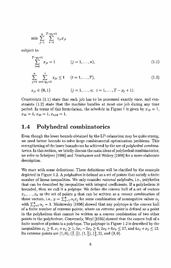
n T-p;+l

min L L CjtXjt j=l t=l

subject to

T-p;+l

L Xjt = 1 (j = 1, ... , n), (1.1) t=l

n t

L L Xjs~l (t=l,".,T), (1.2) j=l s=t-p;+l

Xjt E {0, l} (j = 1, ... , n; t = 1, ... , T - Pj + 1).

Constraints (1.1) state that each job has to be processed exactly once, and con­straints (1.2) state that the machine handles at most one job during any time period. In terms of this formulation, the schedule in Figure 1 is given by x12 = 1, X25 = 1, X3s = 1, X4,10 = 1.

1.4 Polyhedral combinatorics

Even though the lower bounds obtained by the LP-relaxation may be quite strong, we need better bounds to solve large combinatorial optimization problems. This strengthening of the lower bounds can be achieved by the use of polyhedral combina­torics. In this section, we briefiy discuss the main ideas of polyhedral combinatorics; we refer to Schrijver [1986] and Nemhauser and Wolsey [1988] fora more elaborate descri ption.

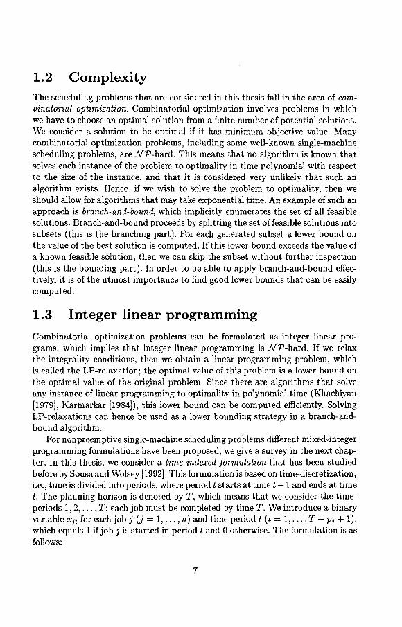
We start with some definitions. These definitions will be clarified by the example depicted in Figure 1.2. A polyhedron is defined as a set of points that satisfy a fini te number of linear inequalities. We only consider rational polyhedm, i.e., polyhedra that can be described by inequalities with integral coefficients. If a polyhedron is bounded, then we call it a polytope. We define the convex hull of a set of vectors x 1, ••• , Xk as the set of points y that can be written as a convex combination of these vectors, i.e., y = I:j=1 ajXj for some combination of nonnegative values aj

with I:j=1 aj = 1. Minkowsky [1896] showed that any polytope is the convex hull of a finite number of extreme points, where an extreme point is defined as a point in the polyhedron that cannot be written as a convex combination of two other points in the polyhedron. Conversely, Weyl [1935] showed that the convex hull of a fini te number of points is a polytope. The polytope in Figure 1. 2 is described by the inequalities x1 ~ 0, x1 + x2 ~ 1, 5x1 - 2x2 ~ 0, 2x1 + 6x2 ~ 17, and 4x1 + x2 ~ 12. lts extreme points are (1, 0), ( t, ~), (1, ~ ), ( ~, 2), and (3, 0).

8

Figure 1.2: A polytope.

We define the affine hull of the set of vectors x 1, ... , xk as the set of points y that can be written as an affine combination of these vectors, i.e., y = EJ=1 O:jXJ

for some combination of values a3 such that Ej=1 aJ = 1. Note that the affine hull of two different points is the line through these points, whereas the convex hull is equal to the line-segment bet.ween these two points. A set x 1, .•• , xk of vectors is called affinely independent if none of these vectors is in the affine hull of the other k - 1 vectors; this is the case if and only if the system of equations Ej=1 a3xj 0 and Ej=1 aJ = 0 has aJ = 0 (j 1, ... , k) as a unique solution. Observe that the maximum number of affinely independent points in a k-dimensional space is (k+ 1 ). The dimension of a polyhedron is the dimension of the smallest affine space that contains the polyhedron. A polyhedron P has dimension kif the maximum number of affinely independent points in Pis (k + 1). We have that fora k-dimensional polyhedron P in nn there are exactly ( n - k) linearly independent equations that are satisfied by all points in P. A polyhedron in 'R..'1 that bas dimension nis called full-dimensional. In order to show that the dimension of a polyhedron p in nn equals k, we have to determine ( n - k) linearly independent equations satisfied by all elements of P and ( k + 1) affinely independent points in P; the first part shows that k is an upper bound on the dimension of P, whereas the second part shows that k is a lower bound. Instead of determining ( k + 1) affinely independent points, one can also determine k linearly independent direction vectors in P, where a direction vector in Pis a vector that can be written as x y for some x, y E P. As the affine independence of the vectors Xj (j = 1, ... k + 1) is equivalent to the linear independence of the vectors Xj - x 1 (j = 2, ... , k + 1), the determination of ( k + 1) affinely independent points boils down to the determination of k linearly independent direction vectors with a fixed endpoint. In many situations it is easier

9

to point out linearly independent direction vectors. The polytope in Figure 1.2 is a polytope in R 2

; its dimension is hence at most 2. Since the vectors (1, 0), (3, 0), and (~,~)are affinely independent, its dimension equals 2, i.e., it is full-dimensional.

Consider an integer linear programming problem given by min{cx 1 x ES}, where S { x 1 Ax :$ b, x ~ 0, x integral } with A and b integral. The LP-relaxation is given bymin{cx 1 Ax :$ b,x ~ O}. Bydefinition, thesetoffeasiblesolutionsofthe LP-relaxation, denoted by PLP, is a polyhedron. lt is easy to see that the optima! value of the integer programming problem min{ ex 1 x E S} satisfies

min{cx 1 x ES} min{ ex 1 x E conv(S)}.

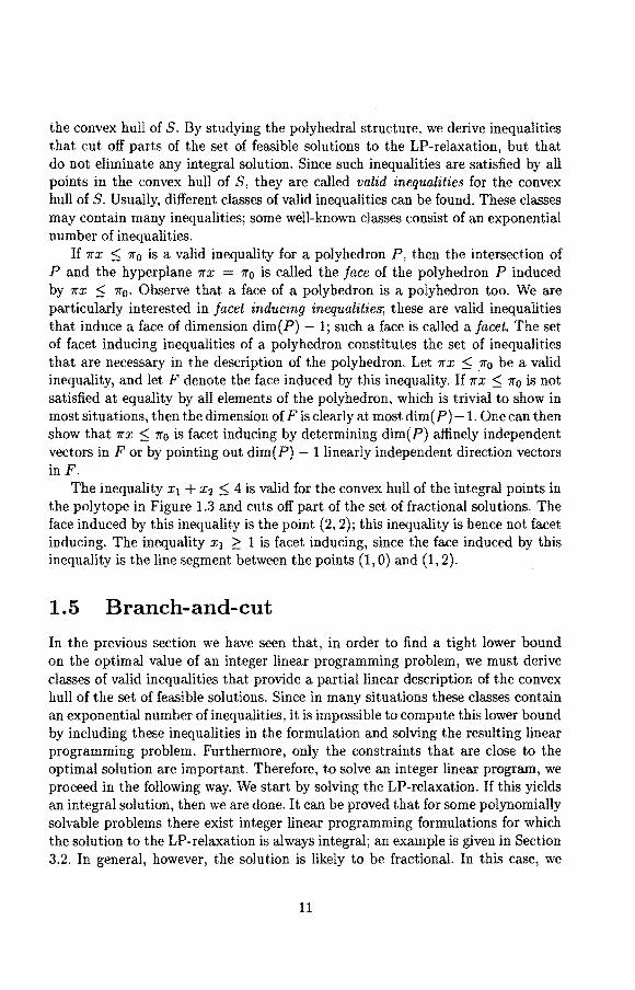
Using resultsof Giles and Pulleyblank [1979], one can show that the convex huil of S is also a rational polyhedron (see Nemhauser and Wolsey [1988]). This polyhedron is clearly contained in PLP. Note that, if we consider a problem in terms of binary variables, then S is finite and the convex hull of S hence is a polytope. In Figure 1.3 the convex hull of the integral points in the polytope of Figure 1.2 is indicated by a dashed quadrangle.

Figure 1.3: The convex hull of the set of integral solutions.

Suppose that we have a linear description of the convex hull of S. Since, by definition, each extreme point of the convex hull is integral, we can solve the integer linear programming problem to optimality through the simplex method, which is known to find an extreme point. In general, however, it is hard to find a linear description of the convex hull of S, which could be expected, since the integer linear programming problem isNP-hard. Therefore, we try to find a partial description of

10

the convex hull of S. By studying the polyhedral structure, we derive inequalities that cut off parts of the set of feasible solutions to the LP-relaxation, hut that do not eliminate any integral solution. Since such inequalities are satisfied by all points in the convex hull of S, they are called valid inequalities for the convex hull of S. Usually, different classes of valid inequalities can be found. These classes may contain many inequalities; some well-known classes consist of an exponential number of inequalities.

If 1rX :::.; 7ro is a valid inequality for a polyhedron P, then the intersection of P and the hyperplane 7rX 7ro is called the face of the polyhedron P induced by 1rX ~ 7r0 . Observe that a face of a polyhedron is a polyhedron too. We are particularly interested in facet inducing inequalities; these are valid inequalities that induce a face of dimension dim(P) - 1; such a face is called a facet. The set of facet inducing inequalities of a polyhedron constitutes the set of inequalities that are necessary in the description of the polyhedron. Let 1rX ~ ,1ro be a valid inequality, and let F denote the face induced by this inequality. If 1rX :::.; 7ro is not satisfied at equality by all elements of the polyhedron, which is trivial to show in most situations, then the dimension of Fis clearly at most dim(P)-1. One can then show that 1rX :::.; 7ro is facet inducing by determining dim(P) affinely independent vectors in F or by pointing out dim(P) - l linearly independent direct.ion vectors in F.

The inequality x1 + x2 ~ 4 is valid for the convex hull of the integral points in the polytope in Figure 1.3 and cuts off part of the set of fractional solutions. The face induced by this inequalit.y is the point. (2, 2); this inequalit.y is hence not facet inducing. The inequalîty x 1 ~ 1 is facet inducing, since the face induced by this inequality is the line segment bet.ween the points (1, 0) and (1, 2).

1.5 Branch-and-cut

In the previous section we have seen that, in order to find a tight lower bound on the optimal value of an integer linear programming problem, we must derive classes of valid inequalities that provide a partial linear description of the convex hull of the set of feasible solutions. Since in many situations these classes contain an exponential number of inequalities, it is impossible to compute this lower bound by including these inequalities in the formulation and solving the resulting linear programming problem. Furthermore, only the constraints that are close to the optima} solution are important. Therefore, to solve an integer linear program, we proceed in the following way. We start by solving the LP-relaxation. If this yields an integral solution, then we are done. It can be proved that for some polynomially solvable problems there exist integer linear programming formulations for which the salut.ion to the LP-relaxation is always integral; an example is given in Section 3.2. In general, however, the solution is likely to be fractional. In this case, we

11

select from the set of known valid inequalities one or more inequalities that are violated by the current fractional solution. Adding these inequalities to our linear programming problem yields a new problem to which the current fractional solution is no longer feasible. We solve this new problem and, in case of a fractional solution, add violated inequalities again. This process is repeated until either an integral solution is found, or until we cannot find any valid inequality that is violated by the current fractional solution. This procedure is called a cutting plane algorithm, since the added inequalities cut off the current fractional solution. The process of finding violated inequalities for a given fractional solution is called separation.

If we do not find an integral solution by just adding cutting planes, then we proceed by applying branch-and-bound. In case of a formulation that uses binary variables, one possible branching strategy is to fix the value of a fractional variable at either 0 or 1. Obviously, there are many other possible branching strategies. It is well known that the choice of a branching strategy has great influence on the per­formance of a branch-and-bound algorithm. U nfortunately, it is difficult to indicate beforehand which branching strategy will perform best. Often, however, it pays off to take the specific structure of the problem into account. A branching strategy partitions the original problem into smaller subproblems that are characterized by one or more additional constraints; for example, if we fix the value of a variable x at 0, then the additional constraint is x 0. For each subproblem we compute a lower bound by applying the cutting plane algorithm to the current formulation includ­ing the additional constraint. For this reason, such a branch-and-bound algorithm is called a branch-and-cut algorithm. Since we can discard any subproblem with a lower bound that is greater than or equal to the value of the best known solution, we are also interested in good integral solutions. These may be found by applying some heuristic, for instance, by transforming a fractional solution into an integral one.

1.6 Column generation

Computational experiments indicate that the time-indexed formulation yields good lower bounds. A limitation to the applicability of these lower bounds in a branch­and-cut algorithm is formed by the considerable amount of time needed to compute them, i.e., the time needed to solve LP-relaxations. This is mainly due to the large number of constraints in the formulation. Empirica! findings indicate that the typical number of iterations needed by the simplex method increases proportionally with the number of rows and only very slowly with the number of columns (see for example Dantzig [1963]); it is sometimes said that for a fixed number of rows the number of iterations is proportional to the logarithm of the number of columns (see Chvátal [1983]). The time-indexed formulation contains n + T constraints and approximately nT variables, where T ? E'J=I Pi· Hence, especially in case of

12

instances with large processing times, we may expect large running times when the linear programming problems are solved through the simplex method.

To reduce the number of constraints we apply Dantzig- Wolfe decomposition. This decomposition proceeds as follows. The set of constraints Ax $ bis partitioned into two subsets, say AO>x $ b(1) and A(2lx $ b(2). We assume that the polyhedron described by the constraints A<2>x $ b(2) is bounded; the boundedness assumption is not necessary and is made purely for simplicity of exposition. Any point satisfying these constraints can hence be written as a convex combination of extreme points, say x = 1::J;=1 Àkxk, with Ef=1 Àk = 1 and Àk ~ 0 (k = 1, ... , K). If we substitute this representation in the objective function and in the constraint set A<llx :5 b(l),

then we obtain a problem in the variables Àk, which is called the master problem and is given by:

K

min I:(cxk)Àk k=l

subject to

K

L(ACl>x1c)Àk $ b< 1>, (1.3) k=l

(1.4)

(k = 1, ... 'I<).

Observe that by this reformulat.ion the number of constraints has been decreased. However, as the number of variables equals the number of extreme points of the polytope A<2>x $ b<2>, it. may have been increased enormously. This does not really matter, though, since the application of Dantzig-Wolfe decomposition enables us to solve the master problem by column generation.

The column generation technique has been developed t.o solve linear programs with a large number of variables. A column generation algorithm always works with a restricted problem in the sense that. only a subset of the variables is taken into account; the variables outside the subset are implicitly fixed at zero. Suppose that we have selected a subset of the columns that yields a feasible restricted problem. From the theory of linear programming it is known that, after solving this restricted problem to optimalit.y, each included variable has nonnegative reduced cost. The reduced cost of the variable À1c is given by

m

cxk - I:(A<1>x1c);u.; v, i=l

13

where u; denotes the dual variable of the ith constraint, and v denotes the dual variable of the convexity constraint. If each variable that is not included in the re­stricted problem also bas nonnegative reduced cost, then we have found an optimal solution to the complete problem. If there exist variables with negative reduced cost, then we have to choose one or more of these variables to be included in the restricted problem. The main idea bebind column generation is that the occurrence of variables with negative reduced cost is not checked by enumerating all variables hut by solving an optimization problem. This optimization problem is called the pri,cing problem and is defined as the problem of finding the variable with minimal reduced cost. This means that we have to find the extreme point xk of the polytope described by the constraints A(2lx ::; b(2) for which cxk :L;~1 (A(I)xk);u; - v is minimal. To solve this problem, we use the structure imposed by the constraints AC2lx ::; b(2), i.e., we consider 'solutions' to the original problem that are feasi­ble with respect to only a subset of the constraints. To apply column generation effectively, it is important to find a good method for solving the pricing problem.

If the column generation algorithm does not find an integral solution, then we proceed by applying branch-and-bound. A branch-and-bound algorithm in which the lower bounds are computed by solving LP-relaxations through column gen­eration is called a branch-and-pri,ce algorithm. Observe that in any subproblem that arises from branching, only columns may be added that correspond to ex­treme points of the polytope A<2lx ::; b(2) that satisfy the constraints defining the subproblem. This leads to a pricing problem with additional constraints that may complicate the problem. Therefore, it is very important to choose a branching strategy that does not deteriorate the structure of the pricing problem too much.

Up to now little attention has been paid to the combination of column and row generation, i.e., the combination of column generation and the addition of valid inequalities. If constraints are added to the master problem, then the dual variables corresponding to these constraints will occur in the reduced cost, and will hence play a role in the pricing problem, which may seriously complicate this problem. In most situations column generation is applied toa problem formulation obtained through Dantzig-Wolfe decomposition. Two kinds of valid inequalities can hence be distinguished: valid inequalities that are obtained from the original formulation and are translated to the reformulation, and valid inequalities that are obtained directly from the reformulation. In Chapter 5, we show that in many cases valid inequalities of the first kind can easily be handled, whereas valid inequalities of the second kind seem harder to deal with.

1. 7 Outline of the thesis

The main goal of our research is to provide basic tools for the development of improved LP-based branch-and-bound algorithms for single-machine scheduling

14

problems. For these problems several mixed-integer programming formulations have been proposed. None of these formulations clearly dominates all others. In Chapter 2, we discuss these different formulations and their respective advantages and disadvantages.

In this thesis, we consider the time-indexed formulation that has been studied by Sousa and Wolsey [1992]. In Chapter 3, we investigate the polyhedral structure of this formulation. We first show that for some special objective functions the LP-relaxation of the formulation solves the problem. The main results presented in this chapter are complete characterizations of all facet inducing inequalities with right-hand side 1 or 2. This chapter is based on Van den Akker, Van Hoesel, and Savelsbergh [1993].

In Chapter 4, we first derive separation algorithms for the classes of inequali­ties that were identified in Chapter 3. Aft.er that, we discuss the development and implementation of a branch-and-cut algorithm for J.jril 2:: WjCj and give computa­tional results. This chapter is based on Van den Akker, Hurkens, and Savelsbergh [1994A].

Due to the fact that the time-indexed formulation contains a large number of constraints and variables, the major part of the computation time of the branch­and-cut algorithm presented in Chapter 4 is spent on solving linear programming problems. lt may hence be worthwhile to solve these problems by column gener­ation. This technique is discussed in Chapter 5. We first show how to solve the LP-relaxation. Then we discuss how to combine column generation and the addi­tion of the facet inducing inequalities that were identified in Chapter 3. We also consider the combination of row and column generation in a more general con­text. We further study the possibility of applying branch-and-bound. Finally, we discuss the application of so-called key formulations, We also give some computa­tional results. This chapter is based on Van den Akker, Hurkens, and Savelsbergh [1994B].

15

16

Chapter 2

Mixed-integer programming formulations for single-machine scheduling problems

2 .1 Introd uction

Recently developed polyhedral methods have yielded substantial progress in solving important NP-hard combinatorial optimization problems. A well-known example is the traveling salesman problem [Padberg and Rinaldi, 1991]. Relatively few pa­pers, however, have been written on polyhedral methods for scheduling problems. lnvestigation and development of such methods is important, because for many NP-hard scheduling problems it is difficult to obtain tight lower bounds. Lower bounds can be used in a branch-and-bound algorithm or may help to determine the quality of solutions obtained through some heuristic. Moreover, the lower bounds obtained by a polyhedral method can often be used to derive good solutions. Most of the research conducted on polyhedral methods for scheduling problems deals with single-machine scheduling problems. For these problems several mixed-integer pro­gramming formulations in terms of different kinds of varia bles have been proposed. None of these formulations clearly dominates all others. In this chapter, we discuss these formulations and their respective advantages and disadvantages.

2.2 Formulations based on completion times

We describe formulations in which the variables represent the completion times Ci of jobs j = l, ... , n. The problem that we use to illustrate this formulation is lll L:,wiCi. Smith [1956] showed that this problem is solved in polynomial time by scheduling the jobs in order of nonincreasing ratio w)p1. The problem can be

17

formulated as follows:

subject to

(j = 1, ... , n),

(i,j = l, ... ,n,i <j).

(2.1)

(2.2)

Constraints (2.1) state that no job can start before time zero. The disjunctive con­straints (2.2) model the machine availability constraints. They state that no two jobs can overlap in their execution. Observe that this formulation is not an integer linear programming formulation; it contains disjunctive constraints instead of in­tegrality constraints. This formulation has been studied by Queyranne [1986]. He shows that a complete description of the convex hull of the set of feasible solutions is given by the inequalities

.L: Pic1 ;::: .L: PiPj (Sç {1,".,n}). (2.3) jES i,jES:i5,j

This description contains an exponential number of inequalities. However, there exists an O(nlogn) separation algorithm for these inequalities.

Queyranne and Wang [1991A] incorporate precedence constraints in the above formulation. Let A denote the set of ordered pairs of jobs between which a prece­dence relation has been specified: (i,j) E A means that job i bas to be processed before job j. These precedence constraints can be included in the formulation by replacing constraint (2.2) for any pair of jobs (i,j) E A by

Ci - C; 2: Pi·

They present three classes of valid inequalities. These classes are associated with parallel decomposition, series decomposition, and Z-induced subgraphs, where a Z­induced subgraph is a subgraph on four points, say v1 , v2 , v3 , v4 with edges ( v1 , v2 ),

(v3 , v4 ), and (v3 , v2 ). The first class consists of the inequalities (2.3). They show un­der which conditions the inequalities in these classes are facet inducing. They con­sider the special case of series-parallel precedence constraints, i.e., 1 lsepal E wiCi. Lawler [1978] showed that this problem is polynomially solvable, and that the general problem llprecl EwiCi is NP-hard. The last result was also obtained by Lenst.ra and Rinnooy Kan [1978]. Queyranne and Wang show that, in case the precedence constraints are series-parallel, the facet-inducing inequalities in the first two classes provide a complete descript.ion of the convex hull of the set of feasible solutions. Note that in this case the precedence graph does not contain Z-induced subgraphs and hence the third class of inequalities does not apply. They present a

18

computational study on the problem with general precedence constraints in a sub­sequent report (Queyranne and Wang [1991B]). In their cutting plane algorithm, they consider inequalities associated with parallel decomposition and a subset of the class of inequalities associated with series decomposition. For all these inequal­ities separation can be performed in polynomial time. In all their test problems the gap between the lower bound obtained by the cutting plane algorithm and the upper bound provided by a feasible solution is less than 1 percent. To find good feasible solutions two heuristics are used; one of these heuristics is based on the optimal solution of the LP-relaxation.

Von Arnim and Schrader [1993] also consider this formulation for the problem l lprecl E wiCi. They study the special case in which the precedence constraints are P4-sparse, which means that in the precedence graph any subset of five jobs contains at most one Z-induced subgraph. Note that this case includes the case of series-parallel precedence constraints. They give three types of valid inequalities and show that these inequalities completely describe the convex huil of the set of feasible solutions. Precedence constraints are also studied by Von Arnim and Schulz [1994]. For general precedence constraints, they present a description of the geometrie structure of the convex huil of the set of feasible solutions that depends on the series decomposition of the precedence graph and prove a dimension formula. They further show which of the inequalities identified by Von Arnim and Schrader [1993] are facet inducing and give a minimal description of the convex huil of the set of feasible solutions for the special case of P4-sparse precedence constraints.

In his pioneering work on scheduling polyhedra, Balas [1985] investigates com­pletion time based formulations for the job shop scheduling problem. As a special case, he considers the problem Ilril EwiCi and derives some facet inducing in­equalities for this problem.

The main advantage of this formulation is that it contains only n variables. This implies that instances with a large number of jobs or with large processing times can be handled by this formulation in the sense that these instances do not yield extremely large linear programs. A disadvantage is that only problems with a linear objective function in the completion times can be modeled in a straightforward way. In other situations, new variables and constraints have to be introduced. If the objective is to minimize the makespan, then we have to represent the makespan by a new variable Cmax and add the constraints Cmax ~ Ci (j = 1, ... , n). lf the objective is to minimize total weighted tardiness, where the tardiness T1 of job j is defined as max{O, Ci - di} fora given due date dh then this can be modeled by adding for each job ja nonnegative variable Ti denoting the tardiness of job j and ad ding the constraints Ti ~ Ci - di (j = 1, ... , n). Observe that, if extra varia bles are added, then the results concerning complete descriptions no langer hold.

19

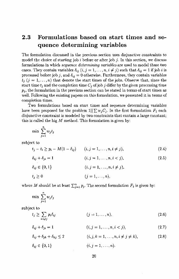
2.3 Formulations based on start times and se­quence determining variables

The formulation discussed in the previous section uses disjunctive constraints to model the choice of starting job i before or after job j. In this section, we discuss formulations in which sequence determining variables are used to model these two cases. They contain variables 8i1 ( i, j = 1, ... , n, i i= j) such that 8;1 1 if job i is processed before job j, and 8;3 = 0 otherwise. Furthermore, they contain variables t1 (j 1, ... , n) that denote the start times of the jobs. Observe that, since the start time tj and the completion time Ci of job j differ by the given processing time Pi, the formulation in the previous section can be stated in terms of start times as well. Following the existing papers on this formulation, we presented it in terms of completion times.

Two formulations based on start times and sequence determining variables have been proposed for the problem 1 l I L, wjCj. In the first formulation F1 each disjunctive constraint is modeled by two constraints that contain a large constant; this is called the big M method. This formulation is given by:

n

min :Ewjt; j=l

subject to

t1 - t; 2:: p; - M(l - 8;1)

{Jij+ bji = 1

8ii E {0,1}

t > 0 J -

(i,j 1, ... ,n,i#j),

( i, j = 1, ... , n, i < j),

(i,j= 1, ... ,n,i#j),

(j 1, ... , n),

where M should be at least L,'J=1 Pi· The second formulation F2 is given by:

n

min LWiti j=l

subject to

tj ;;::: :E p;b;j i:i#j

b;j E {O, 1}

(j l, ... ,n),

(i,j = 1, .. "n, i < j),

(i,j, k = 1, ... , n, i i= j i= k),

(i,j 1, ... , n).

20

(2.4)

(2.5)

(2.6)

(2.7)

(2.8)

Constraints (2.8) state that the order of the jobs defined by the variables óii is acyclic. In formulation F1 this is imposed by the constraints (2.4). Observe that the number of constraints in F1 is of order n2 , whereas the number of constraints in F2 is of order n3 . Therefore, it may be worthwhile to generate the constraints (2.8) as cutting planes. An important disadvantage of formulation F1 is that the big M makes the LP-relaxation very weak: Óij = ~ for all i, j and ti 0 for all j is a feasible solution. Therefore, this formulation is only used as a theoretical concept and not for solving real problems.

For the problem lil L,wiCi, Wolsey [1985] shows that the projection into the t-space, i.e., the subspace spanned by the variables ti, of the polytope described by the constraints

t1 '.2'.: L PiÓij i:i~j

(j = 1, ... , n),

(i,j = 1,".,n,i < j),

(i,j = 1, . .. ,n),

is the convex hull of the set of feasible schedules. In the previous section, we have seen that Queyranne [1986] directly describes this polytope in the t-space. Peters [1988] showed that for this problem constraints (2.8) can be omitted from the LP­relaxation of F2 without changing its optima} value. Nemhauser and Savelsbergh [1992] show that the LP-relaxation of F2 gives the optimal value. Hence, this also holds if the constraints (2.8) are omitted. Note that the last two results are im­plied by the results presented by Wolsey [1985]; they were however established independently. Nemhauser and Savelsbergh fort.her show that the constraints in F2 give a complete description of the convex hull of the set of feasible solutions in the space spanned by the variables t1 and Ó;j· They also show that the inequalities derived in Queyranne [1986] can be written as nonnegative linear combinations of the inequalities in the above linear program.

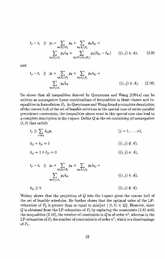
Wolsey [1990] investigates the (t,ó)-formulations for llprecjL,w1C1, i.e., the problem of minimizing the weighted sum of the completion times subject to prece­dence constraints. Precedence constraints can easily be included in the formulation. Again, let A denote the set of pairs (i,j) such that job i has to precede job j. The constraints ó;1 + ó1; = 1 are replaced by óii = 1 and ó1; = 0 for each pair ( i, j) E A. Define Si and P; as the set of successors and predecessors of job j, respectively, i.e., 81 = {kl(j, k) E A} and P1 {kl(k,j) E A}. Wolscy presents the following two classes of valid inequalities:

21

tj - ti > Pi+ I: Pk+ I: Pkóki + kES;nP; kES;\P;

I: PkÓik + I: Pk(6ki - 6ki) ((i,j) E A), (2.9) kEP;\S; kEN\(S;UP;)

and

tj - ti > Pi+ I: Pk+ I: PkÓkj + kES;nP; kES;\P;

I: Pkóik ((i,j) E A). (2.10) kEP;\S;

He shows that all inequalities derived by Queyranne and Wang [1991A] can be written as nonnegative linear combinations of inequalities in these classes and in­equalities in formulation F2 • As Queyranne and Wang fonnd a complete description of the convex hull of the set of feasible solutions in the special case of series-parallel precedence constraints, the inequalities above must in this special case also lead to a complete description in the t-space. Define Q as the set containing all nonnegative (t, 6) that satisfy

tj ~ L Ó;jPi i+/j

tj t; > Pi+ L Pk+ L PkÓkj + kES;nPi kES;\PJ

I: p1;.Ó;k kEP;\S;

Ó·· > 0 •J -

(j=l,".,n),

((i,j) r/: A),

((i,j) E A),

((i,j) E A),

((i,j) fj. A).

Wolsey shows that the projection of Q into the t-space gives the convex hull of the set of feasible schedules. He further shows that the optimal valne of the LP­relaxation of F2 is greater than or equal to min{wt 1 (t, 6) E Q}. However, since Q is obtained from the LP-relaxation of F 2 by replacing the constraints (2.8) with the inequalities (2.10), the number of constraints in Q is of order n2 , whereas in the LP-relaxation of F2 the number of constraints is of order n3 , which is a disadvantage of F2•

22

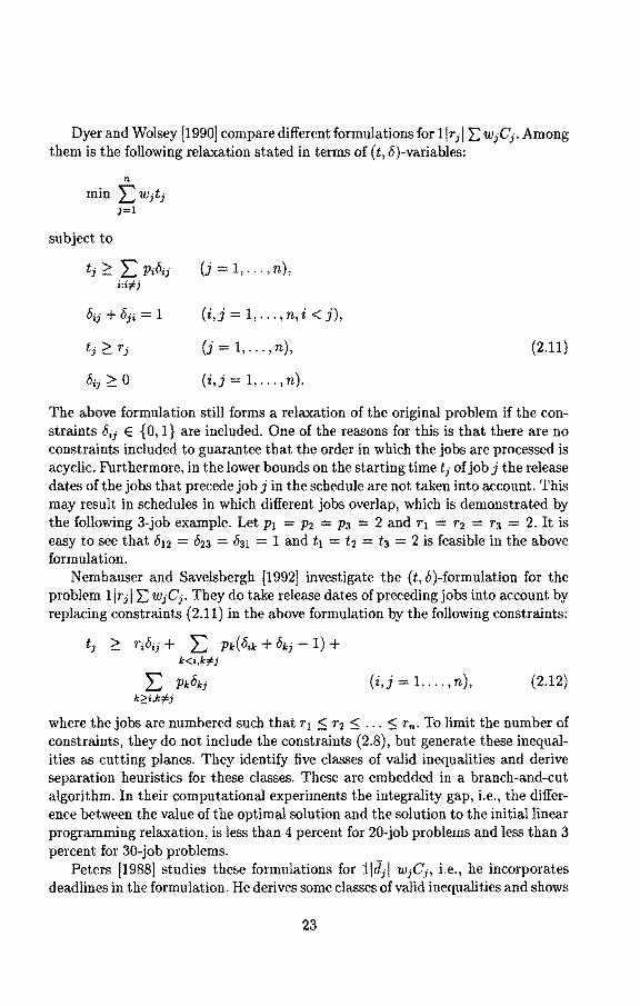
Dyer and Wolsey [1990] compare different formulations for 1lrj1 E WjCj. Among them is the following relaxation stated in terms of (t, 8)-variables:

n

min L:wjtj j=l

subject to

tj?: L Pi8ij i:fr/:j

t· > T· J - J

8" > 0 •J -

(j = 1,.", n),

(i,j = l" .. ,n,i <j),

(j = 1". "n),

(i,j=l, ... ,n).

(2.11)

The above formulation still forms a relaxation of the original problem if the con­straints 8ij E { 0, 1} are included. One of the reasons for this is that there are no constraints included to guarantee that the order in which the jobs are processed is acyclic. Furthermore, in the lower bounds on the starting time tj of job j the release dates of the jobs that precede job j in the schedule are not taken into account. This may result in schedules in which different jobs overlap, which is demonstrated by the following 3-job example. Let p 1 = P2 = p3 = 2 and r1 = r2 = T3 = 2. It is easy to see that 812 823 = 831 = 1 and t1 = t2 = ta = 2 is feasible in the above formulation.

Nemhauser and Savelsbergh [1992] investigate the (t, 6)-formulation for the problem 1Irj1 E Wj Ci. They do take release dates of preceding jobs int.o account by replacing constraints (2.11) in the above formulation by the following constraints:

tj ?: ri8ii + L Pk(8ik +6kj -1) + k<i,k#j

L Pk8kj k"?_i,k#j

(i,j=l,.",n), (2.12)

where the jobs are numbered such that r 1 :5 r2 :5 ... :5 Tn. To limit the number of constraints, they do not include the constraints (2.8), hut generate these inequal­ities as cutting planes. They identify five classes of valid inequalities and derive separat.ion heuristics for these classes. These are embedded in a branch-and-cut algorithm. In their computational experiments the integrality gap, i.e" the differ­ence between the value of the optimal solution and the solution to the initia} linear programming relaxation, is less than 4 percent for 20-job problems and less than 3 percent for 30-job problems.

Peters [1988] studies these formulations for :1.ldil wiCi, i.e" he incorporates deadlines in the formulation. He derives some classes of valid inequalities and shows

23

how to use dominance rules to fix some of the 6-variables. These results are used in the implementation of a branch-and-cut algorithm.

The formulations discussed in this section can be considered as extensions of the formulation discussed in the previous section. The above results indicate that the extended formulations are stronger than the formulation based on completion times; they contain more variables though. The above results further suggest that in this formulation fewer inequalities are needed to obtain a tight lower bound. Consider for example the case in which no release dates, deadlines, or precedence relations have been specified. The set of valid inequalities in terms of this formu­lation that provides a complete description of the convex hull of the set of feasible schedules is of polynomial size; in the formulation based on completion times an exponential number of inequalities is needed. The modeling of the objective func­tions proceeds in the same way as in case of a formulation based on completion times.

Observe that, if we restrict ourselves to the varia bles 6ij, then a feasible solution to the scheduling problem defines a linear ordering. Therefore, valid inequalities for the linear ordering problem (see for example Grötschel, Jiinger, and Reinelt [1985]) are also valid for the (t, 6)-formulation, and hence may also be used in a branch­and-cut algorithm based on this formulation. Miiller [1994] studies the interval ordering polytope, which is an extension of the linear ordering polytope. He shows that the application of some known results on the interval ordering polytope to the linear ordering polytope may help to obtain better lower bounds for single-machine scheduling problems.

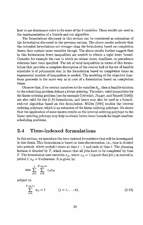
2.4 Time-indexed formulations

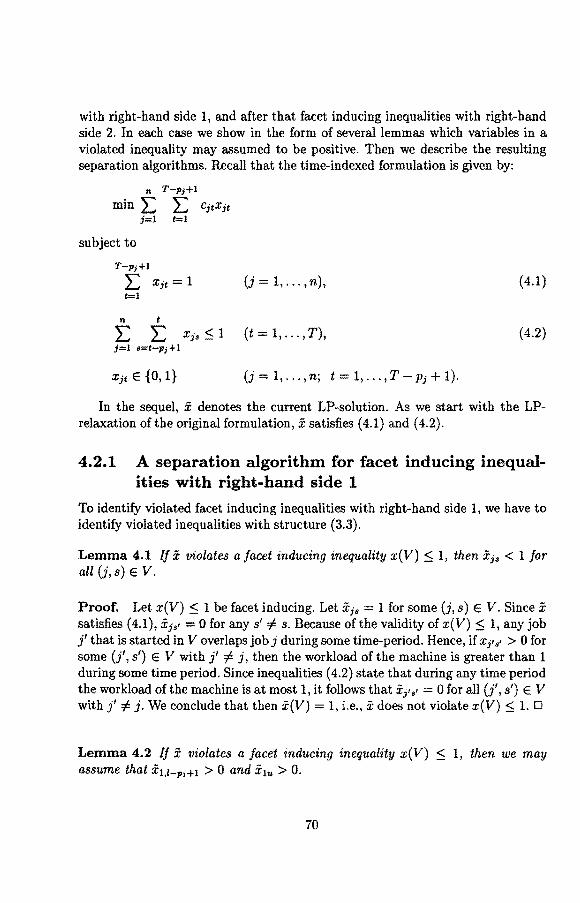
In this section, we introduce the time-indexed formulation that will be investigated in this thesis. This formulation is based on time-discretization, i.e., time is divided into periods, where period t starts at timet - 1 and ends at timet. The planning horizon is denoted by T, which means that all jobs have to be completed by time T. The formulation uses variables Xjt, where Xjt = 1 signals that job j is started in period t; Xjt = 0 otherwise. It is given by:

n T-pi+l

min :E :E CjtXjt j=l t=l

subject to

T-p;+I

:E Xjt = 1 t=l

(j = 1, .. "n), (2.13)

24

n t

L L Xjs 5 1 (t = 1,"., T), (2.14) j=l s=t-p;+l

XjtE{0,1} (j=l, ... ,n; t=l, ... ,T Pi+l).

Constraints (2.13) state that each job bas to be processed exactly once; constraints (2.14) state that the machine handles at most one job during any time period.

Other variants of time-indexed formulations have been considered by Sousa [1989] and Dyer and Wolsey [1990]. They consider a formulation in tenns of variables Y;t. where Y)t = 1 signals that job j is processed during period t; Yit = 0 otherwise. Sousa also considers a formulation in terms of variables Zjt, where Zjt = 1 signals that job j has been started in or before period t; Zjt = 0 otherwise. He shows that these formulations are equivalent to the above formulation in the sense that the associated polyhedra have the same facial structure.

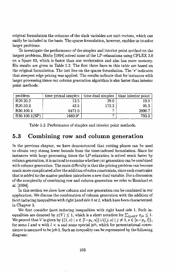
Sousa and Wolsey [1992] introduce three classes of valid inequalities for the time-indexed formulation in terms of the variables Xjt· The first class consists of inequalities with right-hand side 1, whereas the second and third class consist of inequalities with right-hand side k E {2, ... , n}. They show that the inequalities in the first class are facet inducing. Their computational experiments reveal that the bounds obtained from the time-indexed formulation are strong compared to the bounds obtained from other mixed integer programming formulations.

Crama and Spieksma [1993] investigate the formulation in terms of variables Xjt for the special case of equal processing times. They exhibita class of objective functions for which the optimal solution to the LP-relaxation is integral. Further­more, they completely characterize all facet inducing inequalities with right-hand side 1 and present two other classes of facet inducing inequalities with right-hand side k E { 2, ... , n}. These facet inducing inequalities are embedded in a simple cutting plane algorithm. They tested this algorithm on problems with randomly generated cost coefficients Cjt and on the problem llPi = p, ri, djl EwiCi, where the release dates and deadlines may be violated at high cost. Their computational experiments indicate that all classes of inequalities effectively improve the lower bound provided by the LP-relaxation and that the cutting plane algorithm often finds an integral solution.

As mentioned in the previous section, Dyer and Wolsey [1990] compare different formulations for the problem llril EwiCi. They show that Zó::; Zy::; Zx, where Zx and Zy are the optima! values of the LP-relaxations of the formulations in terms of the variables Xjt and Yit respectively, and Zó is the optimal value of the relaxation stated in terms of the (t, 6)-variables that. was present.ed in the previous section.

As the Jatter relaxation may be qui te weak, the above result does not necessarily imply that the time-indexed formulation yields stronger lower bounds than the

25

formulations discussed in the previous two sections. Computational experiments, however, indicate that this formulation does yield strong lower bounds.

A disadvantage of the time-indexed formulation is that it contains a large num­ber of constraints and a large number of variables. There are n + T constraints and approximately nT variables. As T bas to be at least 'L.'J=1 PJ, the formulation is pseudo-polynomial, since its size also depends on the processing times, whereas the formulations in the previous sections are polynomial, since their sizes only depend on the number of jobs. Therefore, to handle instances with a large number of jobs or large processing times we have to consider solution techniques specifically designed for large linear programs.

An advantage of this formulation is that it can be used to model many variants of the nonpreemptive single-machine scheduling problem. We can model all objective functions of the form L.'J=I fJ(tJ) by just setting Cjt = fj(t - 1), whereas in the other formulations we can only deal with cost functions fj(tj) that are linear. If the objective is to minimize the weighted sum of the tardinesses, then we set Cjt Wj(t + Pj dj 1) fort+ Pi - 1 > dj and Cjt = 0 fort+ Pj - 1 :::; dj,

and we do not have to resort to introducing new variables and constraints. If we want to minimize the makespan, then we have to add an extra variable and extra constraints, however. Release dates and deadlines are incorporated in the model by restricting the set of variables. If there are release dates Tj, then we discard the variables Xjt for t l, ... , rj; this means that these variables are implicitly fixed at O. Deadlines are incorporated in a similar way. Therefore, if release dates or deadlines are included, then the convex hull of the set. of feasible solutions is a face of the original convex hull. This means that the set of facet inducing inequalities is contained in the set of facet inducing inequalities for the original problem. To include precedence constraints, we have to add extra constraints. This implies that it is more complicated to incorporate precedence constraints in this formulation than in the previous formulations.

2.5 A formulation based on positional start times and position determining variables

In this section, we discuss the formulation proposed by Lasserre and Queyranne [1992], which is based on positional start times and position determining varia bles. This model is inspired by a control theoretic view of scheduling decisions. In this view, a con trol is applied at discrete time instants specifying which job the machine will start processing. This formulation is based on variables tk, where tk denotes the start time of the kth job, and binary variables u{ indicating which job j is processed in the kth position. The set of feasible schedules is described by the following set of constraints:

26

n

L:u{ 1 (k=l,.",n), (2.15) j=l

(j=l,.",n), (2.16)

n

tk - tk-l - LPiUL1 ;:::: 0 (k=2,""n), (2.17) i=l

u{ E {0,1} (j,k = 1, . .. ,n),

where constraints (2.15) state that one job is chosen at each decision time, con­straints (2.16) state that each job bas to be processed exactly once, and constraints (2.17) state that no two jobs should overlap in their execution. Release dates r1 and deadlines d1 are included in the formulation by introducing the following con­straints:

n

tk - I>1u{;:::: o (k = 1" ."n), (2.18) j=l

n

- tk + 2:::)-PJ + d1)uj. 2'.: 0 (k = l,""n). (2.19) j=l

Lasserre and Queyranne present a characterization of the set of feasible schedules in the subspace spanned by the varia bles u{. For the problem 1 l I E w1C1, they give complete descriptions of the projections of the convex hull of the set of feasible schedules into the subspace spanned by the positional start times, the subspace spanned by the positional completion times, and, for the special case of equal processing times, the subspace spanned by both these sets of variables.

In their computational experiments they compare this formulation and the time­indexed formulation on the basis of two problems. These problems are l lr1, d1 ICma.x• where Cma.x denotes the makespan, and ljr11Lmax, where Lmax denotes the maxi­mum lateness and the lateness L1 of job j is defined as the difference between its completion time and its due date d1. In this formulation the makespan is given by tn + E'J=1 U~Pi· The lateness of the kthjob is given by tk + E'J=1 u{(P1 -d1)· We can model the problem of minimizing maximum lateness by choosing as objective the minimization of the variable L that denotes the maximum lateness and ad ding the constraints L ;:::: tk + E'J=1 u{(p1 - d1) (k = 1, ... , n). For all their test instances, they compute the lower bounds provided by the LP-relaxations of the above for­mulation and the time-indexed formulation. Their results indicate that the bounds are comparable and that for these problems no formulation is clearly superior to the other in terms of the quality of the LP-relaxation.

27

This formulation differs from the previous formulations in the sense that it allows for easy modeling of different types of problems. On the one hand, this formulation can also be used to formulate so-called generic scheduling problems. An example of such a problem is the positional due date problem studied by Hall [1986] and Hall, Sethi, and Sriskandarajah [1991]. This problem has the special feature that a number of deadlines bas been specified at which a given number of jobs must be completed; only the number, and not the identity, of the completed jobs is important. As we have seen, the makespan given by tn + E'J=1 Piu~ is a linear function in this formulation, whereas it is nonlinear in the formulations in the previous sections. On the other hand, the start time of job j is given by E~=I u{tk, w hich is nonlinear. Therefore, the weighted sum of the start times does not seem to admit a simple linear formulation in this model. We have seen that release dates and deadlines can be included in this formulation by the addition of extra constraints. To include precedence constraints we have to add (n 1) extra constraints for each precedence relation: if job i bas to be processed before job j, then this can be modeled by adding the constraints

k-1 uj <'°'ui

k - L,, 1 j=l

(k 2,".,n).

The number ofvariables in this formulation is of the order n 2• Hence, it contains

more variables than the formulation in terms of completion times and fewer vari­ables than the time-indexed formulation. The formulation in terms of start times and sequence determining variables also contains approximately n 2 variables. For the test problems of Lasserre and Queyranne the strength of the LP-relaxation is comparable with the time-indexed formulation, which suggests that for these problems it is more beneficial to use this formulation; objective functions that are linear in the start or completion times of the jobs are however nonlinear in this formulation.

28

Chapter 3

Facets and characterizations

3.1 lntroduction

We present new results for the time-indexed formulation of nonpreemptive single­machine scheduling problems studied by Sousa and Wolsey [1992]; see Section 2.4 fora brief description. Sousa and Wolsey introduce three classes ofinequalities. The first class consists of inequalities with right-hand side 1; the second and third class of inequalities with right-hand side k E {2, ... , n }. In their cutting plane algorithm, they use an exact separation method only for inequalities with right-hand side 1 and for inequalities with right-hand side 2 in the second class; they use a simple heuristic to identify violated inequalities in the third class. Their computational experiments revealed that the bounds obtained are strong compared to bounds obtained from other mixed integer programming formulations.

These promising computational results stimulated us to study the inequalities with right-hand side 1or2 more thoroughly. This has resulted in complete charac­terizations of all facet inducing inequalities with integral coefficients and right-hand side 1 or 2. Since only some of the classes of inequalities used in the computational experiments by Sousa and Wolsey are facet inducing, we expect that our results can be used to improve their cutting plane algorithm for single-machine schedul­ing problems. The development and implementation of a branch-and-cut algorithm based on the identified classes ofinequalities will be discussed in Chapter 4 together with some computational results.

Recall that the time-indexed formulation studied by Sousa and Wolsey [1992] is based on time-discretization, i.e., time is divided into periods, where period t starts at timet 1 and ends at timet. The planning horizon is denoted by T, which means that all jobs have to be completed by time T. The formulation is as follows:

29

n T-p;+l

min L L: CjtXjt j=l t=l

subject to

T-p;+l

L Xjt = 1 (j=l, ... ,n), t=l

n t

L L Xjs:::; 1 (t = 1, ... , T), j=l s=t-p;+I

Xjt E {0, 1} (j 1, ... , n; t 1" .. , T - PJ + 1),

where x jt = 1 if job j is started in period t and x Jt = 0 otherwise. This formulation can be used to model several single-machine scheduling problems by an appropriate choice of the objective coefficients and possibly a restriction of the set of variables. For instance, if the objective is to minimize the weighted sum of the starting times, then we choose coefficients Cjt Wj(t - 1), where w1 denotes the weight of job j; if there are release dates r1, then we discard the variables x11 fort 1, ... , r1.

This chapter is organized as follows. In Section 3.2, we show that in some special cases the LP-relaxation of the time-indexed formulation solves the problem. These are the problems of minimizing the sum of the completion times and the weighted sum of the completion times. For the first one, we prove that the LP-relaxation always has an integral solution. For the second one, the LP-relaxation provides the optimal value of the problem; its optimal solution may be fractional, though. In Section 3.3, we present some basic concepts concerning the polyhedral structure of the time-indexed formulation. In Sections 3.4 and 3.5, we give complete character­izations of all facet inducing inequalities with right-hand side 1 and 2. We conclude this chapter with a brief discussion of related research in Section 3.6.

3.2 Special cases

3.2.1 Minimizing E Ci

We consider the problem of minimizing the sum of the completion times. This problem is solved by sched uling the jobs in order of nondecreasing processing times without idletimeinserted; itis modeled by choosingc1t = t+p1-I (j = 1, ... , n, t = 1, ... , T PJ + 1). We need the following preliminary lemma.

30

Lemma 3.1 Suppose that nm jobs have to be scheduled on m parallel identical machines in such a way that L,'];:1 Ci is minimal. Then for any optimal schedule we have the following: (a) Each machine processes n jobs. (b) For each pair of jobs i and i', if job i is succeeded by fewer jobs on its machine than job i', then Pi ~ Pi'.

Proof. (a) The main idea bebind the proof is that if jobsi1, i 2 , ••• , ik are scheduled on a machine in this order, then the sum of the completion times equals (p;i) + (Pi1 + Pi2) + ... + (Pi1 + Pi2 + ... +Pik)= E;=1(k + 1 - l)pi" i.e., the processing time of the last job is counted once, that of the last hut one job is counted twice, and so on. Suppose that there is a machine that contains more than n jobs. Then there clearly also is a machine processing less than n jobs. It follows from the above observation that the sum of the completion times is decreased by moving the job on the first position on the overloaded machine to the first position on the underloaded machine.

(b) Since job i has fewer successors on its machine than job i', Pi is counted not as often as Pi' in L,j;;-1 Ci. To guarantee optimality, we need Pi ~Pi'· D

Theorem 3.1 IJ the objective function is the sum of the completion times, then the set of optimal solutions to the LP-relaxation of the time-indexed formulation is a face of the convex hull of the set of integral solutions.

Proof. Consider any fractional optimal solution x• of the LP-relaxation of the time-indexed formulation. Let L be the least common multiple of the denominators of the nonzero values in x•.

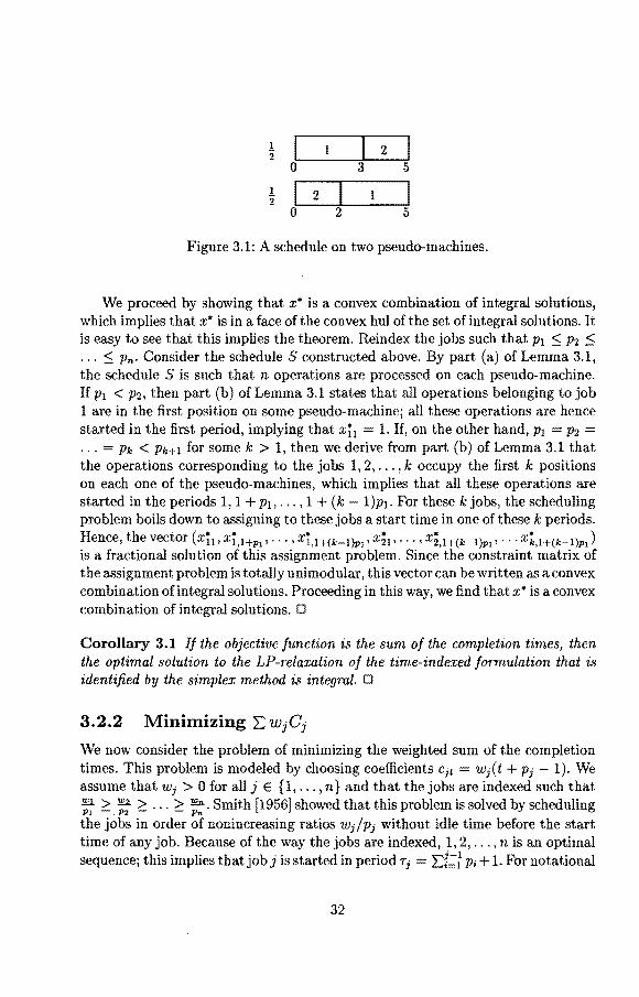
We start with showing that x• corresponds to a schedule on L machines that also minimizes the sum of the completion times. We divide the machine into L parallel pseudo-machines of capacity t each, and each job j into L operations Oii, ... , OiL· Operation Oik has processing time Pi and must be processed on one pseudo-machine without preemption. Operations belonging to the same job are allowed to be processed simultaneously. Each pseudo-machine can process one job at a time. We say that, if xjt = ·Î;. then l operations belonging to job j are started in period ton l different pseudo-machines. In this way, x• corresponds toa schedule Sof the nL operations on the L parallel pseudo-machines. For example, if n = 2,p1 = 3,p2 = 2, and xi1 = ~,xi3 = ~,xh = ~,x24 = ~, then L = 2 and S is the schedule depicted in Figure 3.1.

It is easy to see that the sum of the completion times of the operations Oik

in the schedule S equals L x E'J=1 L,'{'=71+1(t +Pi - l)xit· Hence, the schedule S

minimizes the sum of the completion times of the operations oik·

31

1 1 1 1 2 1 2

0 3 5

l 2 1 2 0 2 5

Figure 3.1: A schedule on two pseudo-machines.

We proceed by showing that x• is a convex combination of integral solutions, which implies that x• is in a face of the convex hul of the set of integral solutions. It is easy to see that this implies the theorem. Reindex the jobs such that p1 ::; p2 ::;

... ::; Pn· Consider the schedule S constructed above. By part (a) of Lemma 3.1, the schedule Sis such that n operations are processed on each pseudo-machine. If p1 < p2, then part (b) of Lemma 3.1 states that all operations belonging to job 1 are in the first position on some pseudo-machine; all these operations are hence started in the first period, implying that xi1 1. If, on the other hand, p1 P2 = ... = Pk < Pk+l for some k > l, then we derive from part (b) of Lemma 3.1 that the operations corresponding to the jobs 1, 2, ... , k occupy the first k positions on each one of the pseudo-machines, which implies that all these operations are started in the periods 1, 1+p1, .•. ,1 + (k l)p1. For these k jobs, the scheduling problem boils down to assigning to these jobs a start time in one of these k periods. H th t ( • • • • • .• ) ence, e vee or x11 , x1,i+pi, .•. , x1.l+(k-l)pi, x21 , ... , x2,i+(k-l)pi, ... xk,l+(k-I)pi

is a fractional solution of this assignment problem. Since the constraint matrix of the assignment problem is totally unimodular, this vector can be written as a convex combination of integral solutions. Proceeding in this way, we find that x• is a convex combination of integral solutions. D

Corollary 3.1 IJ the objective function is the sum of the completion times, then the optimal solution to the LP-relaxation of the time-indexed formulation that is identified by the simplex method is integral. D

3.2.2 Minimizing I; w1C1 We now consider the problem of minimizing the weighted sum of the completion times. This problem is modeled by choosing coefficients Cjt = Wj(t +Pi - 1). We assume that Wj > 0 for all j E {1, ... , n} and that the jobs are indexed such that ;:- 2:: ;: 2:: ... 2:: ~·Smith [1956] showed that this problem is solved by scheduling the jobs in order of nonincreasing ratios wi/Pi without idle time before the start time of any job. Because of the way the jobs are indexed, 1, 2, ... , nis an optimal sequence; this implies that job j is started in period Tj L:f::i Pi+ 1. For notational

32

convenience, we define w_1 = +oo and Wn+i 0. Let ZLP and Z1p be the optima} value of the LP-relaxation and the integer programming problem, respectively.

Theorem 3.2 IJ the objective Junction is Ej=1 WjCj, then (1) ZLP = Z1p,

(2) il ~ > !!!i = ... = ~ > wk±i with i < k, then in any optimal solution to :1 Pi-! Pi Pk Pk+! -

the LP-relaxation the jobs i, i + 1, ... , k are entirely processed during the periods Ti,Ti + 1, ... ,Tk+l -1, i.e., if Xjt > 0 with j E {i,i + 1, ... ,k}, then Ti :5 t :5 Tk+l Pj·

Proof. (1) Observe that, by Smith's rule, the vector x•, which is defined by

* { 1 xit = 0 if t = Tj,

otherwise,

is an optima} solution to the integer programming problem and that the optimal value Z1p is equal to Ej=1 wi(ri + Pj - 1). We will now show that x• is also an optima} solution to the LP-relaxation by defining a feasible solution (u*, v*) to the dual of the LP-relaxation such that x* and ( u*, v*) satisfy the complementary slackness relations.

The dual Dof the LP-relaxation is given by

n T

max 'L:uj + 'L:vt j=l t=l

subject to

t+p1-l

Uj + L V8 :5 (t +Pi - l)wi s=t

We define (u", v*) by

w·+k~ ' Pj

0

Tj+P;-l

uj = (ri +Pi l)w; - L: v; 1=-r;

33

(j = 1, ... , n, t = 1, ... , T- Pi+ 1),

(t = 1, . .. ,T).

ift=rj+k, withjE {l, ... ,n},

k E {0,1, ... ,pj},

n

if t 2: E Pj + 1, j=l

(j = 1,2, ... ,n).

Note that -v; equals the total weight of the work that still bas to be done at the beginning of period t if the jobs are processed in the order 1, 2, ... , n. Note further that v; is defined twice if t = Tj and that both values coincide.

We first show that x* and ( u•, v*) satisfy the complementary slackness relations, i.e., for all t with t = 1, ... , T we have

n t

v;(~= L xjs - 1) = 0 j=I •=t-pj+l

and for all j, t with j 1, ... , n, t = 1, ... , T Pj + 1 we have

t+pj-1

xjt((t + Pj - l)wj - uj - L v;) = 0. •=t

The second relation trivially holds, since xjt is positive only if t = Ti, but then

(t +Pi - l)wj - uj E!!??-1 v; = 0 by definition. As to the first relation, note that, since x• corresponds to a schedule without idle time, Ej=1 E~=t-pj+I xj. 1 for 1 $ t $ Ej=1 Pi· As v; 0 for all t ?::: Ej=1 Pi + 1 by definition, we have that the first relation holds.

What is left to show is that ( u•, v*) is feasible. Clearly, v; $ 0 for all t. We have to show that for all j and for all t

Vj(t) $ lj(t),

where Vj(t) andli(t) aredefinedas Vj(t) = E~!~j-l v; andlj(t) = (t+Pi l)wi-uj. We prove that the above inequality holds by showing below that for each j the piecewise-linear function t'1(t) connecting all values Vj(t) is a concave function that coincides from timet = Ti until timet Tj + 1 with the line ii(t) connecting all values lj(t).

Consider any job j. Observe that for all t with Tj $ t < Tj +Pi = Tj+i, we have v;+ 1 - v; = ~, and that for all t with t 2". Tn+i = E'J=1 Pi + 1, we have vt*+1 - vt• = 0. Since !!!l. > ~ > ... > !!!ll. > 0, we have that the piece-wise linear

p1-p2- -p"

function connecting the values v; is concave. Hence, t'1(t) is a concave function as well, since it is the sum of a finite number of concave functions. The line fi(t) has slope Wj and, by definition, Vj(t) = li(t) fort = Ti· As to the slope of t'1(t) between t = Ti and t Tj + 1, we have

implying that fi(t) and t'1(t) coincide from time Tj until time Tj + 1.

34

We conclude that ( u•, v*) is an optimal solution to D that satisfies the com­plementary slackness relations with x•, which is an optimal solution to the integer programming problem and hence also to the LP-relaxation.

(2) Let x denote any optimal solution to the LP-relaxation. We know from linear programming theory that, since (u*, v*) is an optimal solution to D, x and ( u*, v*) must satisfy the complementary slackness relations. Let i ~ k be such that ;:~: > ~p-· ••• = ~ > wk+i. By definition, we have v;. - v;._1 = w;-i, v;+1 vt• = !::i.

• Pk Pk+I • • P•-1 p,

for all t with ri :5 t < Tk+1, and v~+i+l - v;•+i = ;:;:.Let j be any job from the job set { i, i + l, ... , k}. Since x and ( u•, v*) satisfy the complementary slackness relations, it follows that if Xjt > 0, then Vj(t) = lJ(t). By definition, Vj(t) = lj(t) fort= TJ· For all t with Ti :5 t ~ 7H1 - Pi, we have

Vj(t + 1) - Vj(t) = v;+p· - v; =Pi w; ' Pi

Hence, the points Vj( t) ( r; ~ t ~ rk+1

implies that for all t with r; :5 t ~ Tk+l

Pi+ 1) lie on a line wit.h slope wi, which Pi+ 1 we have

Vj(t) = lj(t).

F\J.rthermore,

Vj(ri)-Vj(r; -1) v;,+P;-l -v;,_1 = (v;,+P;-l -v;;) + (v;, -v;,_1)

( l) W; Wi-1 _ ( l)Wj Wi-1 = Pj - - + -- - Pi - - + > Wj,

Pi Pi-1 Pj Pï-1

and

W; Wk+l Wj + (PJ - 1)- = -- +(Pi -1)- < wi. Pk+l Pi Pk+l Pi

Since "Cj(t) is concave, it follows that for all t with t < T; ort > Tk+l - PJ + 1 we have

Vj(t) < lj(t).

We conclude that, if Xjt > 0, then T; :5 t :5 Tk+l - Pi+ 1. Note that if i k = j, i.e., the value of the ratio ;f is unique, then we find that Xjt can only be positive

for t = TJ or t = Tj + l. We now show that x;t 0 fort= Tk+l - Pi+ l, which implies that in case the

value of the ratio ;f is unique, Xjt can only be posit.ive for t = Tj.

35

Since x and ( u"', v*) satisfy the complementary slackness relations, we have that v;(1 - E~=t-p;+I x3,) = 0 for all t. Since v; < 0 for all t with 1 $ t $ E'J=1 Pi• it must be that E~=t-pj+l xi• = 1 for all t with 1 $ t $ E'J=1 Pi· Hence, although x may be fractional, the machine bas a workload equal to 1 in the time periods 1 until ~~- p ·. Now suppose that !!ll. = !!!2. = ... = .!!!.&. > wo+i • The machine bas

.l.J3-l J ' PI P2 Pk Pk+I

workload 1 during the time periods 1 until P1 + ... +Pk = Tk+I 1. Furthermore, from the above it follows that the jobs j E {1, 2, ... , k} are the only jobs that may have Xjt > 0 for some t with 1 ~ t $ rk+1 -1, i.e., the only jobs that may be started in time periods 1, ... , rk+I - 1. Hence, the jobs 1, 2, ... , k have been completed at the end of time period rk+1 - 1. Proceeding in this way we find that (2) holds. D

Corollary 3.2 IJ the objective fenction is Ej-=1 w3Cj, then (1) if w;- 1 > "!!1.. > w;+1 /or some j E {1, 2, ... , n}, then Xjr = 1 in any optimal

PJ-1 PJ PJ+l J

solution to the LP-relaxation, (2) ij !!ll. > ~ > ... > ~, then the optimal solution to the LP-relaxation is

Pl P2 Pn integral and unique. D

Remark. Theorem 3.2 also holds if we do not rest.riet ourselves to positive weights Wj· Letland m be such that Wj > 0 for j E {1,2, ... ,l}, Wj = 0 for j E {l + 1, ... ,m -1}, and w3 < 0 for j E {m, ... ,n}. We define Tj = Ei<JPi + 1 for j E {1,2" ",m - 1} and Tj = T Eï?_jPi + 1 for j E {m". "n}. The proof proceeds along the same lines if we define v* by

v* t

w·+k"!!.l • Pi

0

j-1 E W; + k"!!.l

i=m PJ

if t = Tj + k with j E {1, 2, .. "l},

k E {O, 1" .. ,pi - 1},

if t = Tj + k with j E { m, " . , n},

kE{O,l,.",pi-1}.

In case of arbitrary weights, the first part of Corollary 3.2 still bolds for all j with wi :f:. 0, but the second part of Corollary 3.2 has to be reformulated as follows: If !!!.l.P > !!!2.P > ... > then the optimal solution to the LP-relaxation is integral and

1 2 Pn unique with the exception of the variables corresponding to a job with wi = 0.

From the above, one might get the impression that the optima! value of the LP­relaxation is always optima! for any scbeduling problem that can be modeled by this formulation and that is solvable in polynomial time. The following instance of

36

the problem lldil E Ci shows that this is not the case. Smith [1956] showed that this problem is solved in O(nlogn) time by the following backward scheduling rule: schedule in the last position the job with the largest processing time that is allowed to be completed there. Consider the following 3-job example with T = 20, Pi 1, P2 = 3, and Pa 10, and d1 = d2 20 and d3 = 13. By the above rule, the optima! integral solution is xu = x2,12 = x32 = L For this schedule we have

Ei'=l cj = Ei=l E[=7;+l(t +Pi l)Xjt = 26. However, Xu = X12 = X13 l, X21 = l, x2,14 ~'and x34 = 1 is a feasible solution to the LP-relaxation and has

Ej"'1 E;:7;+i ( t +Pi - 1 )Xjt 22Ï · This shows that the optimal value of the LP­relaxation can be strictly smaller than the optima! value of the original problem.

3.3 Basic properties of the polyhedral struc­ture

In the time-indexed formulation, the convex hull of the set of feasible schedules is not full-dimensionaL As it is often easier to study full-dimensional polyhedra, we consider the polyhedron P that is associated with an extended set of solutions and defined by

T-p;+l

L Xjt ~ 1 (j = 1," "n), (3.1) t=l

n t

L L Xjs ~ 1 (t=l, ... ,T), (3.2) j=l •=t-p;+l

Xjt E {0, 1} (j=l, ... ,n; t=l, •.. ,T-pi+l).

In this relaxation we no langer demand that each job has to be started. Although it may seem more natura} to relax the equations into inequalities with sense greater­than-or-equal instead of less-than-or-equal, we have chosen for the lat.ter option, since it has the advantage that the origin and the unit vectors are elements of the polyhedron, which is often convenient for dealing with affine independence. For instance, it is not hard to show that the inequalities Xjs ~ 0 are facet inducing. Note that the collection of facet inducing inequalities for the polyhedron associated with the extended set of solutions includes the collection of facet inducing inequalities for the polyhedron associated with the original set of solutions. In this chapter, we say that any feasible solution to the above formulation is a feasible schedule, even though not all jobs have to be processed.

Before we present our analysis of the structure of facet inducing inequalities with right-hand side 1 or 2, we introduce some notation and definitions.

37

The index-set of variables with nonzero coefficients in an inequality is denoted by V. The set of varia bles with nonzero coefficients in an inequality associated with job j defines a set of time periods Vj = { sl(j, s) E V}. If job j is started in period s E Vj, then we say that job j is started in V. With each set Vj we associate two values

and

Uj max{sls E Vj}.

For convenience, let li = oo and Uj = -oo if Vj 0. Note that if Vj ::f:: 0, then li is the first period in which job j can be finished if it is started in V, and that ui is the last period in which job j can be started in V. Furthermore, let l = min{li IJ E

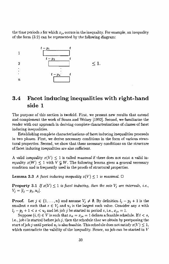
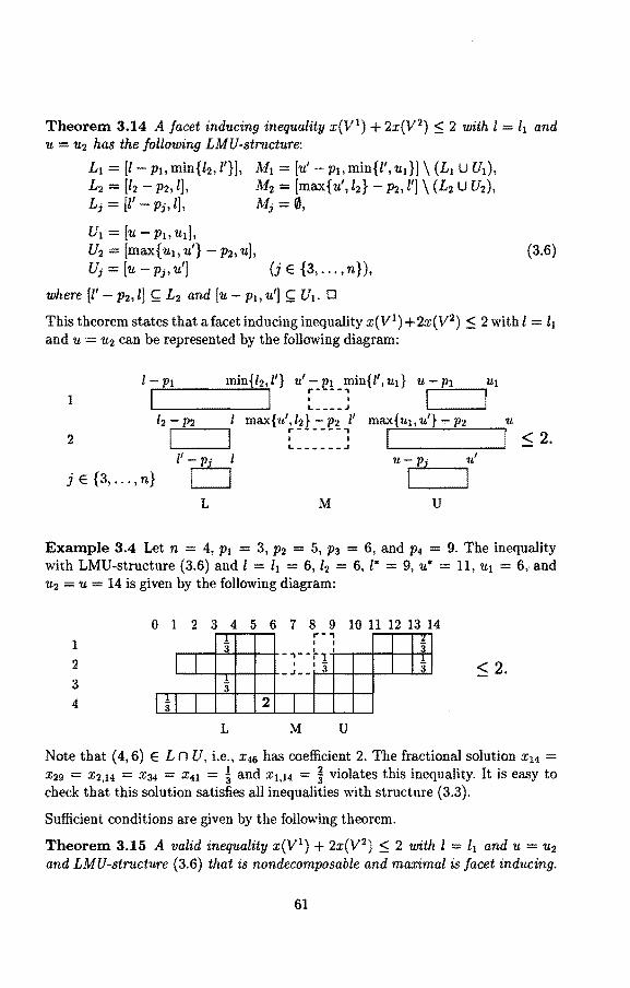
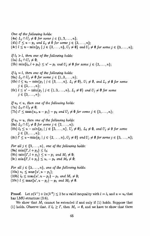
{l,"., n}} and u = max{ uill E {l" .. , n}}. We define an interval [a, b] as the set of periods { a + 1, a + 2, ... , b}, i.e" the set

of periods between time a and time b. If a ~ b, then [a, b] = 0.

Lemma 3.2 A facet inducing inequality ax ::::; b with integral coefficients ajs and integral right-hand si de has either b ? 0 and coefficients ai• in { 0, 1, ... , b} or is a positive scalar multiple of -xi• ::::; 0 for some (j, s) with 1 ::::; s ::::; T Pi+ 1.

Proof. Since the origin is an element of the polyhedron, any valid inequality ax $ b must have a nonnegative right-hand side. Since the schedule x defined by Xjs 1 and Xj's' = 0 for all (j', s') ::f:: (j, s) is feasible for every (j, s ), a valid inequality ax $ b does not have coefficients greater than b. We now show that a facet inducing inequality does not have negative coefficients, unless it is a positive scalar multiple of -xi• ::::; 0. Let ax ::::; b be a valid inequality with ai• < 0. Let x be any feasible schedule with Xjs = 1. lf Xjs = 1 is replaced by Xjs = 0, then the schedule remains feasible and ax is increased. Therefore, any feasible schedule such that ax = b satisfies Xjs = 0. Since Pis full-dimensional, it follows that the inequality ax $ b cannot be facet inducing, unless ax =bis equivalent to Xjs = 0, i.e., ax $ b is a positive scalar multiple of -Xjs ::; 0. D

Observe that this lemma implies that the inequalit.ies Xjs ~ 0 are the only facet inducing inequalities with right-hand side 0. For presentational convenience, we use x(S) to denote E(j,s)ES Xjs· As a consequence of the previous lemma, valid in­equalities with right-hand side 1 will be denoted by x(V) ::::; 1 and valid inequalities with right-hand side 2 will be denoted by x(V 1

) + 2x(V2) ::::; 2, where V = V1 u V 2

and V 1 n V2 = 0. Furthermore, we define Vj2 {si (j, s) E V 2}.

In the sequel, we shall often represent inequalities by dîagrams. A diagram contains a line for each job. The blocks on the line associated with job j indicate

38

the time periods s for which Xjs occurs in the inequality. For example, an inequality of the form (3.2) can be represented by the following diagram:

3.4 Facet inducing inequalities with right-hand side 1

The purpose of this section is twofold. First, we present new results that extend and complement the work of Sousa and Wolsey [1992]. Second, we familiarize the reader with our approach in deriving complete characterizations of classes of facet inducing inequalities.

Establishing complete characterizations of facet inducing inequalities proceeds in two phases. First, we derive necessary conditions in the form of various struc­tural properties. Second, we show that these necessary conditions on the structure of facet inducing inequalities are also sufficient.

A valid inequality x(V) S 1 is called maximal if there does not exist a valid in­equality x(W) S 1 with V ~W. The following lemma gives a general necessary condition and is frequently used in the proofs of structural properties.

Lemma 3.3 A facet inducing inequality x(V) S 1 is maximal. D

Property 3.1 /f x(V) S 1 is facet inducing, then the sets Vj are intervals, i.e., Vj= [lj - Pi, Ujl·

Proof. Let j E {l, ... , n} and assume Vj #- 0. By definition li - Pi+ 1 is the smallest s such that s E Vj and ui is the largest such value. Consider any s with li - Pi + 1 < s < ui and let job j be started in period s, i.e., Xjs = 1.

Suppose (i, t) E Vis such that Xit = Xjs = 1 defines a feasible schedule. Ift < s, i.e" job i is started before job j, then the schedule that we obtain by postponing the start of job j until period ui is also feasible. This schedule does not satisfy x(V) S 1, which contradicts the validity of the inequalit.y. Hence, no job can be started in V

39

before job j. Similarly, we obtain a contradiction if t > s, which implies that no job can be started in V after job j.

We conclude that choosing Xjs = 1 prohibits any job from starting in V. Be­cause of the maximality of x(V) ;:; 1, we must have (j, s) E V. D

Property 3.2 Let x(V) :::; 1 be facet inducing. (a) Assume l = l1 :::; l2 = min{ljlJ E {2, ... , n}}. Then Vi = [l - p1,l2] and Vj= [lj - Pi, l] for all j E {2, ... , n}. (b) Assume u = u1 2: u2 = max{uilJ E {2, ... , n}}. Then Vi = [u2 - P1,u] and Vj= [u - Pi, ui] for all j E {2, ... , n}.

Proof. (a) Let x(V) $ 1 be facet inducing with l = li $ l2 min{lj 1 j E {2, ... , n} }. Observe that Property 3.1 implies that Vi is an interval and that by definition its lower bound equals l - p1. We now show that the upper bound is equal to l2. Since X2.12-p2+1 1 and x1• = 1 defines a feasible schedule for any s > l2, we have that only one of these variables can occur in x(V) $ 1; as by definition (2, h - p2 + 1) E V, it follows that the upper bound of Vi is at most l2. Now, let X1s = 1 for some s E [l - PI, l2]. Reasoning as in the proof of Property 3.1 we can show that since l - PI + 1 E Vi it follows that no job can be started in V aft.er job 1. As s $ l2 = min{ljlJ E {2, ... , n} }, it is impossible to start any job in V before job 1. From the maximality of x(V) $ 1 we conclude that Vi = [l - p1 , l2]. Similar arguments can be applied to show that Vj [li - Pi, l] for all j E {2, ... , n}.

The proof of (b) is similar to that of (a). D

Observe that by Property 3.2(a) a facet inducing inequality x(V) $ 1 with l = l1

necessarily has uI = u. Consequently, Properties 3.2(a) and 3.2(b) can be combined to give the following theorem.

Theorem 3.3 A facet inducing inequality x(V) $ 1 has the following structure:

Vi = [l - pi, u], Vj= [u - P1 1 l] (j E {2, ... ,n}),

(3.3)

where l = l1 $ u1 = u. D

This theorem states that a facet inducing inequality with right-hand side 1 can be represented by the following diagram:

l - PI u

1 1

u-pi l :::; 1. j E {2, ... ,n} l 1

40

Note that if Vj= 0 for all j E {2, ... ,n}, l =PI, and u = T- PI+ 1, then the inequalities with structure (3.3) coincide with the inequalities (3.1 ); if l = u, then the inequalities with structure (3.3) coincide with the inequalities (3.2).

Example 3.1 Let n = 3, PI = 3, p2 = 4, and p3 = 5. The inequality with structure (3.3), l = lI = 6 and u = uI = 7 is given by the following diagram:

1

2

3

2 3 4 5 6 7

m ~ 1.

Note that the fractional solution XI 4 = x17 = x33 = ! violates this inequality.

Sousa and Wolsey [1992] have shown that the given necessary conditions are also su:fficient.

Theorem 3.4 A valid inequality x(V) :'.S 1 with structure (3.3) that is maximal is facet inducing. D

Specific necessary and su:fficient conditions for a valid inequality x(V) :'.S 1 with structure (3.3) to be maximal are given by the following theorem. In the proof we use the following observation. If a valid inequality x(V) :'.S 1 is maximal, then for any (j, s) et V there must be a feasible schedule with Xjs = 1 and x(V) = 1. We call such a schedule a counterexample for (j, s ).

Theorem 3.5 A valid inequality x(V) :'.S 1 with structure (3.3) is maximal if and only if Vj =fa 0 for some j E {2, ... , n}, or x(V) :'.S 1 is one of the inequalities (3.1), i.e., l =PI and u .= T - PI+ 1.

Proof. Let x(V) :'.S 1 be a valid inequality with structure (3.3). Let x(V) :'.S 1 be maximal and suppose that Vj = 0 for all j E {2, ... , n }. It is not hard to see that x(V) :'.S 1 must be one of the inequalities (3.1), and hence l = PI and u = T - PI+ 1. On the other hand, it is easy to see that if Vj =fa 0 for some j E { 2, ... , n}, then there is a counterexample for any (j, s) et V. Hence x(V) :'.S 1 is maxima!. Analogously, if x(V) :'.S 1 is one of the inequalities (3.1), then it is maximal. D

41

3.5 Facet inducing inequalities with right-hand side 2

In the previous section, we have derived a complete characterization of all facet inducing inequalities with right-hand side 1. We now derive a similar characteriza­tion of all facet inducing inequalities with right-hand side 2.

First, we study the structure of valid inequalities with right-hand side 2 and coeffi­cients 0, 1, and 2. Consider a valid inequality x(V1) + 2x(V2) $ 2. Clearly, at most two jobs can be started in V. Let j E {l, ... , n} and s E lf;. It is easy to see that, if job j is started in period s, at least one of the following three statements is true.

(i) It is impossible to start any job in V before job j, and at most one job can be started in V af ter job j.

(ii) There exists a job i with i # j such that job i can be started in V before as well as after job j and any job j' with j' # j, i cannot be started in V.

(iii) At most one job can be started in V before job j, and it is impossible to start any job in V after job j.

Therefore, we can write V = L U MU U, where L Ç Vis the set of variables for which statement (i) holds, M Ç V is the set of variables for which statement (ii) holds, and U Ç Vis the set of varia bles for which statement (iii) holds. Analogously, we can write V; = Li u Mi u Ui. No te that each of the sets L1, Mi> and U1 may be empty.

lf job j is started in a period in ~2 , then it is impossible to start any job in V before or after job j. lt follows that ~2 Ç Lj n Ui for all j, and hence V 2 Ç L n U. It is not hard to see that if Li i- 0 and Ui i- 0, then the minimum of Li is less than or equal to the minimum of Uj, and the maximum of Lj is less than or equal to the maximum of Ui. By definition Lj n Mi= 0 and Min Ui 0. The set M consists of periods between the maximum of Li and the minimum of U1 and hence M1 must be empty if Li n Uj i- 0. By definition, of the sets Land U, x(L) $ 1 and x(U) $ 1 are valid inequalities.

We conclude that a valid inequality x(V1) + 2x(V2 ) $ 2 can be represented by a collection of sets L1, M1, and Ui. To derive necessary conditions on the structure of facet inducing inequalities with right-hand side 2, we study this LMU-structure more closely.

A valid inequality x(V1 ) + 2x(V2) $ 2 is called nondecom.posable if it cannot be

written as the sum of two valid inequalities x(W) $ 1 and x(W') ::::;; 1. A valid

42

inequality x(V1) + 2x(V2) :5 2 is called maximal if there does not exist a valid

inequality x(W1) + 2x(W2

) :5 2 with V Ç W, V2 Ç W 2, where at least one of the

subsets is a proper subset. The following lemma yields a general necessary condition and will be used frequently to prove structural properties.

Lemma 3.4 A facet inducing inequality x(V1) + 2x(V2 ) :5 2 is nondecomposable

and maximal. D

The remaining part of the analysis of the LMU-structure proceeds in two phases. In the first phase, we derive conditions on the structure of the sets L and U by considering them separately from the other ~ts. The structural properties thus derived reveal that we have to distinguish three situations when we consider the overall LMU-structure, based on how the sets L and U can be joined. In the second phase, we investigate each of these three situations and derive conditions on the structure of the set M.

Property 3.3 IJ x(V1) + 2x(V2) :5 2 is facet inducing, then the sets L1, M1, and uj are intervals.

Proof. Let j E {l, ... , n} and assume L1 i 0. By definition l; - PJ + 1 is the smallest s such that s E Lj. Let 8 1 denote the largest such value. Consider any 8

with l; - Pi + 1 < s < 8 1 and let job j be started in period 8, i.e., Xjs = 1. Reasoning as in the proof of Property 3.1, we can show that from 8 1 E L; it

follows that no job can be started in V before job j. Suppose (ii. t 1), (i2 , t2) E V with s < t 1 and 8 < tz are such that Xjs = Xi 1t1 Xi2t 2 = 1 defines a feasible schedule. Then the schedule obtained by startingjob j in period l1 Pi+ 1 instead of in period 8 is also feasible, which contradicts l; - Pi+ 1 E L;. Hence, at most one job can be started in V af ter job j.

We conclude that if XJs = 1, then no job can be started in V before job j and at most one job can be started in V after job j. Because of the maximality of x(V1) + 2x(V2 ) :5 2, we must have s E L; and Li hence is an interval. Analogously, the sets MJ and U1 are intervals. D

Consider a facet inducing inequality x(V1) + 2x(V2

) :5 2. We have seen that V 2 Ç L n U. Observe that if job j is started in LJ n U;, then it is impossible to start any job in V before or after job j. Since x(V 1) + 2x(V2 ) :5 2 is maximal, this implies V/ = Li n u1 for all j, i.e., V 2 = L n U.

Property 3.4 Let x(V1) + 2x(V2 ) :5 2 be facet inducing. (a) Assume l l1 :5 l2 :5 min{l1 1 j E {3, ... , n}}. Then L1 = [l - P1, h] and L1 = [l1 - Pi• l] for all j E {2, ... , n }. Furthermore, there exists a j E {2,.", n} such that L1 i 0.

43

(b) Assume u = u1 2 u2 2 max{ui li E {3, ... ,n}}. Then Ui= [u2 p1iu] and Ui= [u -pj, u1] for all j E {2, ... , n}. Furlhermore, there exists a j E {2, ... , n} such that Ui #= 0.

Proof. (a) Let x(V1) + 2x(V2 ) S 2 be facet inducing with l = l1 S l2 S min{lj 1

j E { 3, ... , n}}. No te that by definition l - p1 + 1 E Vi. Since the earliest possible completion time of a job started in Vis l, we must have l - p1 + 1 E L1• Reasoning as in the proof of Property 3.2, we find that Li is an interval with lower bound equal to l - p1 and with upper bound at most equal to l2. Now, let xis = 1 for some s E [l p1, l2]. As in the proof of the Property 3.3, we can show that from l - p1 + 1 E L1, it follows that at most one job can be started in V after job l. Since s s l2 , it is impossible to start any job in V before job 1. Because of the maximality of x(V1) + 2x(V2 ) s 2, we conclude that s E Lj and hence L 1 = [l - p1, l2]. Similar arguments can be applied to show that Lj [lJ PJ, l] for all j E {2, ... , n }.

Now suppose Lj = 0 for all j E {2, ... , n}. We show that in this case x(V1) +

2x(V2) s 2 can be written as the sum of two valid inequalities with right-hand side 1, which contradicts the fact that x(V1) + 2x(V2

) s 2 is facet inducing. Define W {(1,s) 1 s E L1 n Ui} u {(j,s) 1 j E {2" .. ,n}, s E Vj} and W' = {(1, s) 1 s E Vi}. We first show that EsEV; Xjs S 1 is a valid inequality. For all j E {2" .. , n} we have, since by assumption Lj = 0, li Pi 2 l, i.e., s > l for all s E Vj. Consequently, if Xji 81 = x32. 2 = 1 defines a feasible schedule such that Ej=2 EsEV; Xjs = 2, then X1,1-v1+1 = XJis 1 = X32 82 1 also defines a feasible schedule, which contradicts the validity of x(V1) + 2x(V2 ) s 2. Hence, Ej=2 EsEV; Xjs S 1 is a valid inequality and it easily follows that x(W) S 1 is also valid. Clearly, x(W') s 1 is a valid inequality and x(W)+x(W') x(V1 )+2x(V2).

We conclude that x(V1) + 2x(V2) s 2 is not facet inducing. Hence, Lj #= 0 for some jE{2, ... ,n}.

The proof of (b) is similar to that of (a). D

Like the proof of Theorem 3.5, many of the proofs of the properties and theorems presented in this section use counterexamples. If x(V 1) + 2x(V2) s 2 is facet inducing, then, since x(V1

) + 2x(V2) s 2 is maximal, for any (j, s) <f. V there is a feasible schedule such that Xjs = 1 and x(V1 ) + 2x(V2 ) = 2. We call such a schedule a counterexample for (j, s).

Property 3.5 Let x(V1) + 2x(V2 ) S 2 be facet inducing. (a) Assume l = l1 s l2 S l*, where l* = min{lj 1 j E {3, "., n}}. Then for all j E {3, ... ,n} such that L1 #= 0 we have l1 = l*, and for all j E {3, ... , n} such that L1 = 0 we have t• - Pi 2 l, i.e" L1 = [l*" - P;, l] Jor all j E {3". "n}. (b) Assume u = u1 2 u2 2 u*", where u* = max{ u1 1 j E {3" ", n }}. Then for all j E { 3" .. , n} such that Ui #= 0 we have u1 = u*, and Jor all j E { 3, . " , n} such that UJ = 0 we have u* s u p1, i.e., U1 = [u p1, u*] Jor all j E {3, ... , n}.

44

Proof. (a) Let x(V 1) + 2x(V2) $ 2 be facet inducing with l = 11 $ l2 $ l*. By

definition of l* and Property 3.4, Li Ç [l* - Pi• l] for all j E {3, ... , n }. We assume without loss of generality that l* = l3• Suppose that Li ::/= [l* - Pi, l] for some j E { 4, ... , n }, say L4 ::/= [l* - p4, l]. Clearly, if l* - p4 ;::: l, then L4 = 0 and hence L4 = [l* - p4 1 l]. Consequently l* - p4 < land l4 > l*, i.e., l* - p4 + 1 f/. l14. Since x(V1) + 2x(V2 ) $ 2 is maximal, there is a counterexample for ( 4, l* p4 + 1 ). Let X4,1•-p4+1 = xii•i = x32.2 = 1 define such acounterexample. Since l*-p4 +1 $ l, the jobsji andj2 are started after job4. Clearly one of the jobs 1, 2, and 3does not occur in {j1, h}; suppose that it is job 3. It is now easy to see that X3,1•-p3+1 = Xj1 s 1 = Xj282 = 1 is afeasibleschedule, which contradicts thevalidityof x(V 1 )+2x(V2) $ 2. If job 1 or job 2 does not occur in {ji, h} we obtain a contradiction in the same way.

The proof of (b) is similar to that of (a). O

Properties 3.4 and 3.5 state that if x(V1) + 2x(V2

) $ 2 is facet inducing and we assume l = li $ l2 $ l*, then the set L can be represented by the following diagram:

1

2

j E {3" .. , n}

Similarly, if we assume u u1 ~ u2 ;::: u•, then the set U can be represented by the following diagram:

1

u - P2 u2

2 1 1

u - Pi u•

j E { 3" .. , n} !.....______.

Observe that a facet inducing inequality with right-hand side 2 bas at most three types of intervals L3, each characterized by the definition of the first period of the interval, and at most three types of intervals Uj, each characterized by the defini­tion of the last period of the interval. Stated slightly differently the intervals Lj have the same structure for all jobs hut two. Similarly, the intervals U3 have the same structure for all hut two jobs. It turns out that, when we study the overall

45

LMU-structure, it suffices to consider three situations, based on the jobs with the deviant intervals Lj and Ui:

(la) l = l1 < l2::; l* and u u1 > u2 ;::: u*, where l* = min{lj 1 j E {3,.", n}} and u* = max{ui Ij E {3, ... , n}};

(1 b) l = li < l2 ::; l*, u = u1 > U3 ;::: u•, and lj > l2 or ui < u3 for all j E {2, ... , n }, where t• min{li Ij E {3, ... , n}} and u• = max{uj Ij E {2,4, ... ,n}};

Before we investigate each of the three situations, we prove a property that applies to case 1.

Property 3.6 IJ x(V1 )+2x(V2) ::; 2 is facet inducing with l l1 < '2 = min{li 1

j E {2, ... , n}} and u u1 >ui max{ui 1 j E {2, .. "n}}, then l2 <ui.

Proof. Suppose that l2 ;::: ui. We show that x(V1) + 2x(V2 ) ::; 2 can be written as the sum of two valid inequalities with right-hand side 1, which contradicts the fact that x(V1

) + 2x(V2) ::; 2 is facet inducing. Let W = { (1, s) 1 s E L1 n U1 } U { (j, s) 1

j E {2, ... ,n}, s E Vj} and W' = {(1,s) 1 s E Vi} U {(j,s) 1 j E {2, ... ,n}, s E Li n Ui}· Clearly x(W) + x(W') = x(V1) + 2x(V2 ) and x(W') ::; 1 is a valid inequality. From Vj Ç [lj - Pi, uil Ç [l2 - Pi• u;] for all j E {2, ... , n} and h ;::: u;, it easily follows that L:sEV; Xjs ::; 1 is a valid inequality and hence x(W) ::; 1 is also valid. D

3.5.1 Case {la)

Observe that the conditions on li and ui and Properties 3.4 and 3.5 completely determine the sets Land U. Therefore, all that remains to be investigated is the structure of the set M.

Property 3. 7 IJ x(V1) + 2x(V2 ) ::; 2 is facet inducing with l = l1 < '2 ::; l* and u = u1 > u2 ;::: u*, then we have that M1 [u* - p1 , l*] n [l2 , u2 - p1],

M2 [u* P2, t•]n [l, u - P2] n [h - p2, u2], and Mi [u2 Pi, l2] n [l, u - Pil /or jE{3"",n}.

Proof. Let x(V 1) + 2x(V2

) ::; 2 be facet inducing with l = l1 < l2 ::; l* and u = u1 > u2 ;::: u*. lf job 1 is started in M 1 , then, since li ::; l* and u2 ~ u•, it should be possible to start job 2 in V before as well as after job 1, which implies that M1 Ç [h, u2 - pi]. Furthermore, it should be impossible to start any job j E {3, ... , n} in

46

V and hence MI Ç [u* - PI, l*]. We conclude that M1 Ç [u* - PI, l*] n [l2, u2 - p1]. If job 1 is started in period s E [u* pi, l*] n [l2, u2 P1], then, since s E [l2, u2 - P1L [l2, u2-P1] C [l pi, u], and L2nU2 = [u P2, l], job 2 cannot be started in L 2 nU2•

Sincex(V1)+2x(V2) $ 2 is maximal, itfollows that M 1 = [u* -p1, l*]n [12, u2-p1]. By definition M2 Ç [l2 - p2, u2j. If job 2 is started in M 2, then, since l l1

and u = ui, it should be possible to start job 1 in V before as well as after job 2, which implies that M 2 Ç [l, u - p2]. Furthermore, it should be impossible to start any job j E {3, .. "n} in V and hence M2 Ç [u* - p2, r]. We conclude that M2 Ç [u* - p2, l*] n [l, u - p2] n [12 p2, u2]. If job 2 is started in period s E [u* - P2, l*J n [l, u - p2] n [l2 - P2, u2], then, since s E [l2 - P2, u2] and L1 n U1 = [u2-p1, 12],job 1 cannot be startedin L1 nU1. Sincex(V1)+2x(V2) $ 2 ismaximal, it follows that M2 = [u* - P2, l*] n [l, u P2] n [l2 - P2, u2].

Let j E { 3, ... , n}. If job j is started in M" then it should be possible to start job 1 in V before as well as after job j, which implies that Mi Ç [l, u Pil· Furthermore, it should be impossible to start any job j' E {2, 3, ... , n} \ {j} in V and hence Mi Ç [u2 - Pi, l2]. We conclude that Mj Ç [u2 - Pi, l2] n [l, u - Pi]. If job j is started in period s E [u2 -pi, l2] n [l, u-pi], then, since s E [u2 -pi, l2], LI nU1 = [u2 p1, l2], and, by Property 3.6, h < u 2, job 1 cannot be started in L1 n U1. Since x(V1

) + 2x(V2) $ 2 is maxima!, it follows that Mi [u2 Pi> l2] n [l, u - Pil·

Observe that by definition Mk Ç [lk - Pk, uk] for all k E {1, ... , n} and that for all but k = 2 this condition is dominated by other conditions. D

Properties 3.4, 3.5, and 3. 7 completely determine the LMU-structure of a facet inducing inequality x(V 1)+2x(V2 ) $ 2 with l = l1 < 12 $ l* and u = u1 > u2 2: u*. However, in order to emphasize the inherent structure of the intervals Mi, we prefer to use a different representation of the set M. It is easy to show that, if x(V1) + 2x(V2

) $ 2 is facet inducing with l l1 < l2 $ l* and u = uI > u2 2: u•, then for all j E {3, ... , n} we have [u2 - Pi• l] Ç Li and (u Pi• l2] Ç Ui. We can use this observation to show that Properties 3.4, 3.5, and 3.7 can be combined to give the following theorem.

Theorem 3.6 A facet inducing inequality x(V1) + 2x(V2 ) :S 2 with l = 11 < l2 :S l* and u = u 1 > u2 ;::: u* has the following LMU-structure:

LI = [l - PI, l2J, M1 = [u* - Pi. l*] \ (L1 U U1), L2 = [l2 - P2, l], M2 [max{ u*, l2} - P2, min{l*, u2}] \ (L2 U U2), Li = [l* - Pi, l], Mi= [u2 Pi, l2] \ (Li U Ui),

U1 = [u2 P1i u], U2 = [u P2, u2], Ui= [u-pj,u*] (j E {3,.",n}),

where [u2 - Pi, l] Ç Lj and [u PJ, l2] Ç Ui for all j E {3" .. , n}. D

47

(3.4)

This theorem states that a facet inducing inequality x(V1) + 2x(V2) S 2 with

l = l1 < l2 S l* and u = uI > u2 2 u* can be represented by the following diagram:

l-p1 /2 u* - PI l* U2 - u r----, 1 1 1

1. - - - - .J l2 - P2 l max{u*,12} p2 min{l*,u2} u - P2 u2

1 1

"------, 1 1 $; 2. 2 1 1

'-------.J

j E {3, ... ,n} l* - p · 1 u2 - Pi

Ö "., 1 1

... · t2 L M u

Example 3.2 Let n = 4, PI 3, P2 5, p3 6, and p4 = 9. The inequality with LMU-structure (3.4) and l lI 7, l2 9, l* 12, u* 14, u2 = 16, and u = uI = 19 is given by the following diagram:

3 4 5 6 7 8 9 10 11 12 13 14 15 16 17 18 19 "., 1

1 1 1 1

I,".ï"ï

2 ~äJ __ ~_J < 2. 3 " -, 4 2 1 1

... - .J

L M u Note that the fractional solution XIs xI,19 = X2,10 x2,16 = X4,4 = Î violates this inequality. It is easy to check that this solution satisfies all inequalities with structure (3.3).

Suffi.cient conditions are given by the following theorem.

Theorem 3. 7 A valid inequality x(V1) + 2x(V2 ) S 2 with l = l1 < l2 S l* and

u = u1 > u2 2: u* and LMU-structure (3.4) that is nondecomposable and maximal is facet inducing.

Proof. Let x(V 1) + 2x(V2 ) :S 2 be a valid inequality with l = l1 < l 2 S l* and u = u1 > u2 2 u* and LMU-structure (3.4) that is nondecomposable and maximal, and let F = {x E Plx(V1) + 2x(V2) = 2}. We show that dim(F) = dim(P) -1 by exhibiting dim(P) l linearly independent direction vectors in F; a direction vector in Fis a vector d = x y with x, y E F. For notational convenience, a direction vector will be specified by its nonzero component.s. We give three sets of direction vectors: unit vectors dj• 1 forall (j, s) ~ V, d1• = 1, vectorsdI,1-pi+l = d2" 2 -1

48

for all (j, 8) E V2, and a set of IV l - IV2 I - 1 linearly independent direction vectors dit•i = 1, dJv2 = -1 with (ji, 81), (h 82) E V\ V 2• Together these give dim(P)-1 linearly independent direction vectors in F.

If (j, 8) <f. V, then, since x(V1) + 2x(V2) ~ 2 is maximal, there is a counterex­ample for (j, 8) defined by, say, Xjs = XiJsi = x3282 1. Clearly this schedule is an element of F. Note that the schedule Yiisi = y3282 = 1 also is an element of F and hence d = x - y yields the direction vector djs = 1.

Note that for (j, 8) E V2 the schedule defined by Xjs 1 is an element of F. Since l < l2 and, by Property 3.6, l2 < u2, we have that Y1,l-pi+l = Y2u2 = 1 defines a feasible schedule. This schedule also is an element of F and hence djs = 1, d1,1-p1+i = d2u2 = -1 is a direction vector in F for all (j, 8) E V 2.

We determine the IVI IV21 - 1 direction vectors dit•i = 1, d32•2 -1 with (ji, 8 1), (j2, 8 2 ) E V \ V 2 in such a way that the undirected graph G whose vertices are the elements of V \ V 2 and whose edges are given by the pairs { (j 1, 8 1), (j2 , 8 2)}

corresponding to the determined direction vectors is a spanning tree. This implies that the determined direction vectors are linearly independent.

Observe that dj1•1 = 1, d32s2 -1 with U1, 81), U2, 82) E v \ v2 is a direction vector in F if there exists an index (i, t) E V \ V 2 such that XJisi Xit = 1 and y32.2 = Yit = 1 both define feasible schedules. In this case, we say that dii•i = 1, dj2 s 2 = -1 is a direction vector by (i, t).

First, we determine direction vectors that correspond to edges in G within the sets { (j, 8) 1 8 E (Li u Mi) \ U1} and { (j, 8) 1 8 E UJ \ Li}. For 8 - 1, 8 E L1 \ Ui, di,s-1 = -1, d1. = 1 is a direction vector by (2, u2). If M1 =/:- 0, then d112 = -1, dim = 1 is a direction vector by (2, u2), where mis the minimum of Mi, and for 8 - 1, 8 E Mi, di,s-l = -1, d1• = 1 is a direction vector by (2, u2). Furthermore, for 8 - 1, 8 E U1 \ L1, di,s-I = -1, d18 1 is a direction vector by (2, l2 - P2 + 1). Now, let j E {2, ... , n }. For 8 - 1, 8 E Li \ Uj, dj,s-I = l, di• = 1 is a direction vector by (1, u). If Mj =f:. 0, then dj1 = -1, dim = 1 is a direction vector by (1, u), where mis the minimum of Mj, and for 8 - l,8 E Mj, dj,s-l = -1,djs = 1 is a direct.ion vector by (1, u). Furthermore, for 8 1, 8 E Uj \ Lj, d1,s-1 -1, d1• = 1 is a direction vector by ( 1, l - p1 + 1).

Second, we determine direction vectors that. correspond to edges in G between sets {(j,8) 1 8 E (L1 u M1) \ Uj} belonging to different jobs and bet.ween sets {(j,8) 1 8 E Uj \ L1} belonging to different jobs. We define W = {(l,8) 1 8 E L1 nUi}u{(j,8) jj E {2,".,n}, 8 E Yj} and W' {(1,8) 18EYj}U{(j,s)1 j E {2,".,n},s E Li n Uj}· Clearly x(W) + x(W1

) = x(V1) + 2x(V2) and

x(W1) ~ 1 is a valid inequality. Since x(V1 ) + 2x(V2

) ~ 2 is nondecomposable, there must be a feasible schedule such that x(W) = 2, i.e., L:seV; Xjs = 2. Let Xjis 1 = x32•2 1 with 8 1 < s2 define such a schedule. It is easy to see that we may assume s 1 lii -pii + 1 and s2 = u32. Since l = li, Yi,1-p1 +1 = Yhuh = 1 also defines a feasible schedule, it follows that di,t-p1+1 = -1,dJi,lii-Pii+l = 1 is a direction vector by U2, s2). In the same way, since u = ul> YJi,lii-Pii +1 = Y1 ... = 1 defines a

49

feasible schedule, it follows that d1u = -1, d12u; = 1 is adirection vector by (j1, s1). For j E {2, ... , n} \ {ji} such that Lj U Mi #= 0, d31,1;

1-Ph +l = -1, dj,li-Pi+1 1 is

a direction vector by (1, u). Furthermore, for j E {2, ... , n} \ {h} such that Uj #= 0, dhuh = -1, dJu; = 1 is a direction vector by (1, l - p1 + 1 ).

Finally, we determine a direction vector that corresponds to an edge in G be­tween L U Mand U. Since x(V1) + 2x(V2 ) ::; 2 is nondecomposable and x(U) ::; 1 is a valid inequality, there exists a feasible schedule with x(L) + x(M) 2. Let Xj181 = x12•2 = 1 define such a schedule. Since l1 = l, we may assume without loss of generality that J1 = 1. Since s2 E L32 U Mh, Yhs2 = Y1u = 1 also is a feasible schedule. It follows that dJs1 = -1, d1u = 1 is a direction vector by (j2, s2).

It is easy to see that the determined direction vectors form a spanning tree of G and we hence have determined IVl- IV2 l-1 linearly independent direction vectors. D

Specific necessary and sufficient conditions fora valid inequality with l = l1 < l2 :5 l* and u = u1 > u2 ;:::: u* and LMU-structure (3.4) to be nondecomposable and maxima! are given in the following two theorems.

Theorem 3.8 A valid inequality x(V1) + 2x(V2 ) :5 2 with l l1 < l2 :$. l* and u = u1 > u2 ;:::: u* that has LMU-structure (3.4) is nondecomposable ij and only ij MJ #= 0 j or some j E { 1, ... , n}, and l* < u2 or l2 < u •.

Proof. Let x(V1) + 2x(V2 ) :$. 2 be a valid inequality with l l1 < l2 :$. l* and u = u1 > u2 ;:::: u* that has LMU-structure (3.4).

Suppose that x(V 1) + 2x(V2) :$. 2 is nondecomposable. Since x(L) :$. 1 and x(U) :5 1 are valid inequalities, we must have Mi #= 0 for some j E {l, ... , n }. Suppose l* 2:: u2 and l2 ;:::: u*. Let W = {(1, s) 1 s E L1 n Ui} U {(j, s) 1 j E {2, ... ,n}, s E Vj} and W' {(1,s) 1 s E Vi} U {(j,s) 1 j E {2, ... ,n}, s E LjnUJ}· Clearly x(W)+x(W') = x(V1 )+2x(V2

) and x(W')::::; 1 is valid. Observe that Vi Ç [l2 - p2,u2] and, for j E {3,""n}, Vj Ç [l* PJ,u*] Ç [u2 - Pi 1 l2]. Since, by Property 3.6, l2 < u2, it follows that 'L'J= 2 LsEV; Xj 8 :S. 1 is valid and hence x(W) :::; 1 is also valid, which yields a contradiction. This implies that l* < u2 or l2 < u*.

Suppose that Mi #= 0 for some j E {1, ... , n}, and l* < u2 or lz < u•. Let Wand W' besuch that x(W)+x(W') = x(V 1 )+2x(V2) and x(W) :S. 1 and x(W') :::; 1 are valid inequalities. We assume without loss of generality that (1, l p1 + 1) E W. Note that Xu-p1+1 = X2u2 = 1 is a feasible schedule. The validity of x(W) :::; 1 and (1; l p1 + 1) E W imply that (2, u2 ) E W'. We conclude that, since l < u 2

and (1,l p1 +1) E W, we have (2,u2) E W'. We show that (l,u) E W' and (2,h P2 + 1) E W. By assumption either l* < u2 or l2 < u•. Suppose l* < u2. Note that in this case U2 #= 0 and Lj #= 0 for some j E { 3, ... , n}. Since l* < u2

and (2,u2) E W', we have (j,l* - Pj + 1) E W for all j E {3". "n} such that

50

Li # 0. Furthermore, since l* < u2 < u, it follows that (1, u) E W', and since l2 < u2 < u, it follows that (2, h - P2 + 1) E W. Analogously, (2, l2 - p2 + 1) E W and (1,u) E W' ifl2 < u*.

By assumption Mi # 0 for some j E {1, ... , n }. Suppose that Mj -=f:. 0 for some j E {2, .. "n }. If job j is started in Mi, then job 1 can be started in V before or after job j. If s E Mj, then, since x1,1-p1+1 = Xjs 1 is a feasible schedule and (1, l-p1+1) E W, it follows that (j, s) E W'. We find thatxjs = x1u lisafeasible schedule such that x(W1

) 2, which yields a contradiction. We conclude that from (1, l p1 +1) E W, (1, u) E W' and Mi -=f:. 0, it follows that x(V1) + 2x(V2 )::;; 2 is nondecomposable.

Suppose that M1 # 0. If job 1 is started in M 1 t.hen job 2 can be started in V before as well as after job 1. As int.he previous case, from (2, l2 - P2 + 1) E W, (2, u2) E W', and M1 -=f:. 0, it follows that x(V1) + 2x(V2)::; 2 is nondecornposable. D

Theorem 3.9 A valid inequality x(V1) + 2x(V2) ::; 2 with l = l1 < l2 ::; l* and u = u1 > u2 ;::: u*, that has LMU-structure (3.4) is maximal if and only if each of the following eight hold:

(1) IJ u* < l2 and l < l2 P2, then L1 n U1 # 0;

(2) IJ u2 < l* and u2 < u p2, then L1 n U1 # 0; One of the following holds: (3a) LJ n U1 # 0 /or some j E {2,.", n}; (3b) l::; u* p2 and L2 # 0 and U1 # 0 /or some j E {3, ... , n}; (3c) l::; u2 rnin{pj / j E {3, ... , n}, Lj # 0} and U2 # 0 and L1 # 0 /or some

jE{3,".,n}; .

One of the following holds: (4a) Lj n Ui# 0 /or some j E {2, .. "n}; ( 4b) l* ::;; u - P2 and U2 # 0 and Lj # 0 /or some j E { 3, ... , n}; (4c) l2 ::; u min{pi 1 j E {3, ... , n}, Uj # 0} and L2 # 0 and Uj # 0 /ar some

j E {3" .. , n};

One of the following holds: (5a) Li n U1 # 0; (5b) min{l2, l + p2}::; u* - p1 and Ui# 0 /or some j E {3"." n}; (5c) min{l2, l + P2}::; u - min{pj 1 j E {3, ... , n}, Mi# 0} and Mi# 0 /ar

some j E {3, ". ,n};

One of the following holds: (6a) L1 n U1 # 0; (6b) l* ::; max{ u2, u P2} - P1 and Lj # 0 /ar some j E {3, ... , n }; (6c) l ::;; max{ u2, u P2} - min{pj IJ E {3" ", n }, Mi # 0} and M1 # 0 /ar

somej E {3, .. "n};

51

For all j E { 3, ... , n}, one of the following holds: (7a) min{t•, l +Pi} S u2 - Pi and Mi # 0; (7b) min{z•,z +Pi} S u - P2 and M2 # 0; (7c) min{l",l +pi} :S l2;

For all j E { 3, ... , n}, one of the following holds: (Ba) l2 :S max{u*, u - Pi} - Pi and M1 # 0; (Bb) l :S max{u*, u - Pi} - P2 and M2 # 0; (Be) u2 :S max{u•, u - Pi}·

Proof. Let x(Vi) + 2x(V2) S 2 be a valid inequality with l = l1 < '2 :S l* and

u u1 > u2 ~ u* thathasLMU-structure (3.4). Observethatx(V1)+2x(V2 ) S 2 is maximal if and only if it is impossible to extend any of the intervals Lj, Mi and uj.

First, we show that M1 cannot be extended. If l2 < u* pi, i.e" [12 , u* - pi] # 0, then x2,12 -p2 +1 = xis = Xju• = 1 defines a counterexample for (1, s) for all s E [l2, u* - pi], where j E {3, ... , n} is such that ui u*. If l* < u2 - p1 , i.e., [l*, u2-Pd # 0, then Xj,l•-pi+l = X1s = X2u2 = 1 defines acounterexample for (1, s) fors E [l*, u2 - p1], where j E {3, ... , n} is such that lj = l*. Hence, M1 cannot be extended. In the same way we can show that the intervals Mi with j E { 3, ... , n} cannot be extended.

We show that M 2 cannot be extended if and only if (1) and (2) hold. Suppose that (1) does not hold, i.e., u* < h, l < l2 p2, and L1 n U1 0. Clearly (2, l2 - P2) <f. V. Let job 2 be started in period h P2· Since l* > h, it is impossible to start a job j E {3, ... , n} in V before job 2. Since u* < l2 , it is impossible to start a job j E { 3, ... , n} in V after job 2. Clearly, job 1 cannot be started in L1 n U1, and we find that M 2 can be extended by l2 p2 • In the same way, if u2 < l*, u2 < u - p2, and L1 n U1 = 0, then M2 can be extended by u2 + 1.

Now, suppose that (1) and (2) hold. Suppose u* ~ l2 , i.e., [l,max{u*,l2 }

P2] = [l, u* - P2]. If l < u* - P2, then X1,1-p1+1 = X28 = Xju• = 1 defines a counterexample for (2,s) for all s E [l,u* - p2], where j E {3, ... ,n} is such that ui = u•. Suppose that u* < l2, i.e., [l, max{ u•, l2} - P2] = [l, l2 - p2]. If l < '2 - P2, then, by (1), Li n U1 # 0 and X2s = x112 = 1 defines a counterexample for (2, s) for all s E [l, '2 p2]. Hence, there is a counterexample for (2, s) for all s E [l, max{u*, '2}-p2]. In thesameway, wecanshowthat thereisacounterexample for (2, s) for all s E [min{l*, u2}, u P2]. We conclude that M 2 cannot be extended.

Clearly, the upper bound of L1 cannot be increased. The lower bound of L1

cannot be decreased if and only if there is a counterexample for (1, l - pi). Such a counterexample is given by a feasible schedule xi,1-p1 = Xjs = 1 with (j, s) E V 2

or by a feasible schedule X1,1-P1 = Xji 81 = Xj282 = 1 with (ji, s1), (j2, s2) E V \ V2•

Observe that if j E {2, ... 'n} is such that Lj n uj # 0, then X1,l-PI Xjl 1 defines a counterexample for (1, l P1 ). We find that there is a counterexample of the first type if and only if (3a) holds. Consider a counterexample of the second

52

type. Since u2 2'.: max{ ui 1 j E { 3, ... , n}}, we may assume that job 2 occurs in this counterexample, i.e., the counterexample contains job 2 and a job j 1 E {3, ... , n }. Suppose that job 2 is started before job j 1. It is easy to see that job 2 is started in L2• So L2 # 0 and job 2 is started in period l. Furthermore, job j 1 is started in Uil. Hence, l $ u* - P2 and Uli # 0. We find that there is a counterexample of the second type such that job 2 is started before job j 1 if and only if {3b) holds. If job 2 is started after job j 1 , then job j 1 is started in period land job 2 in U2• Job j 1 may be chosen such that Pii = min {Pi 1 j E { 3, ... , n}, Li # 0}. We find that there is a counterexample of the second type such that job 2 is started after job j 1 if and only if {3c) holds. We conclude that the lower bound of L 1 cannot be decreased if and only if (3) holds. Analogously, U1 cannot be extended if and only if (4) holds.

Clearly, L 2 cannot be extended if and only if there is a counterexample for (2, l 2 - p2) if L 2 # 0, and a counterexample for (2, l) if L 2 = 0, i.e" if and only if there is a counterexample for {2, y- p2 ), where y = min{l2, l + p2}. The proof that there is such a counterexample if and only if (5) holds, is similar to the proof that there is a counterexample for (1, l - pi) if and only if {3) holds. Analogously, U2

cannot be extended if and only if (6) holds. Let j E {3". "n}. It is easy to see that Li cannot be extended if and only

if there is a counterexample for (j,y - Pi), where y = min{l*,l + p3}. Suppose y $ h. If L1 n U1 # 0, then Xj,y-p1 = x112 = 1 defines a counterexample for (j, y p3). lf L1 n U1 = 0, i.e" h $ U2 pi, then Xi,Y-Pj = X112 X2u2 defines such a counterexample. Hence, if y $ [z, then there is a counterexample for (j, y - p3).

Now, suppose y > l2 • Since x(U) $ 1, in any counterexample at least one job is started in L U M. If xi,u-P; = 1, then job 1 and 2 are the only jobs that can be started in L u M. It is now easy to see that a counterexample for {j, y Pi) contains job 1 and job 2, and we find that there is such a counterexample if and only if (7a) or {7b) hol ds. Analogously, the intervals Ui with j E { 3, ... , n} cannot be extended if and only if (8) holds. D

3.5.2 Case (lb)

As in case (la), the conditions on l1 and ui and Properties 3.4 and 3.5 completely determine the sets L and U. From these properties we can easily derive that, if h = l* and u3 = u*, then L; # 0 and U; # 0 for all i such that p; = max{p3 1 j E {2, ... , n} }. But then l; l2 and U; u3 , and we are in case (la). We conclude that l2 < l* or u3 > u*. All that remains to be investigated is the structure of the set M.

Property 3.8 IJ x(V 1 ) + 2x(V2) $ 2 is facet inducing with l = l1 < lz $ l*, u = u1 > u3 2'.: u*, and l3 > l2 or ui< U3 /or allj E {2"",n}, then M1 = 0, M2 = [u3-p2,l*]n[l,u-p2]n[lz-p2,u*], M3 = [u*-p3,l2]n[l,u-p3)rî[l*-p3,u3], and M3 = [u3 -p3,h] n [l,u - p3] /or j E {4, ".,n}.

53

Proof. Let x(V1) + 2x(V2 ) :::; 2 be facet inducing with l = l1 < l2 :::; l*, u u1 > u3 ;;::: u*, and li > l2 or ui < u3 for all j E {2, ... , n }. If job 1 is started in V and it is possibletostart ajobin V beforejob 1, then, since '2 = min{li 1 j E {2, ... , n}}, job 2 can be started in V before job L If it is possible to start a job in V after job 1, then, since u3 = max{ uj 1 j E {2, ... , n} }, job 3 can be started after job 1. This implies that M 1 = 0.

By definition M 2 Ç [l2 - p2 , u•]. If job 2 is started in M 2 , then, since l = l1

and u = u1, it should be possible to start job 1 in V before as well as after job 2, which implies that M 2 Ç [l, u p2]. Furthermore, it should be impossible to start any job j E {3, ... , n} in V and hence M 2 Ç [u3 - p2 , l*]. We conclude that M2 Ç [u3 - P2, l*] n [l, u P2] n [l2 - P2, u*]. If job 2 is started in period s E [u3-p2, l*]n[l, u-P2]n[l2-p2, u•], then, since s E ['2-P2, u•], L 1 nU1 [u3-P1, l2], and u3 ;;::: u•, job 1 cannot be started in L 1 n U1. Since x(V1) + 2x(V2 ) :5 2 is max­imal, it follows that M2 [u3 - P2, l*] n [l, u - P2] n [l2 p2, u•]. Analogously, M3 = [u• - p3, l2] n [l, u p3] n [l* p3, u3] and Mi = [u3 - Pi, l2] n [l, u - Pil for j E {4, ... ,n}. D

Properties 3.4, 3.5, and 3.8 determine the LMU-structure of a facet inducing in­equality x(V1) + 2x(V2) :::; 2 with l = l1 < l2 :::; l*, u = u1 > u3 ;;::: u•, and li > l2 or ui < u3 for all j E {2, ... , n }. As in case (la), we prefer to use a different representation of the set M in order to emphasize the inherent structure of the intervals Mi. It turns out that a facet inducing inequality x(V1) + 2x(V2 ) s 2 with l = l1 < l2 :5 l*, u u1 > u3 2 u•, and li < l2 or ui < U3 for all j E {2, ... , n} bas the following property, which restricts the class of inequalities determined by Properties 3.4, 3.5, and 3.8 and leads toa simpler form of the intervals Mi.

Property 3.9 IJ x(V1) + 2x(V2 ) ::::; 2 is facet inducing with l = l1 < l2 s t•,

u = u1 > u3 2 u•, and li > l2 or ui < u3 /or all j E {2, .. "n}, then l* :5 u*.

Proof. Let x(V1) + 2x(V2) s 2 be facet inducing with l = l 1 < 12 s l*, u = u1 > U3 2 u•, and li > l2 or Uj < u3 for all j E {2, ... , n }. To be able to prove that l* S u•,wefirstshowthat[u3-p2,min{l*,u3}] Ç \/2and[max{u*,l2}-p3,l2] Ç V3. It is easy to see that if job 2 is started in [u3 - p2, min{ l*, u3}], then it is impossible to start any job j E {3, ... , n} in V and job 1 cannot be started in L1 n U1.

Since x(V1) + 2x(V2) :5 2 is maximal, it follows that [u3 - p2,min{l*,u3}] Ç \/2. Analogously, [max{ u•, l2} - p3, l2] Ç V3. Since, by assumption, li > l2 or Uj < U3 for all j E {2," "n }, we have [3 > l2 and u2 < u3. From [u3 p2, min{[•, u3}] Ç V2 and u2 < u3, we conclude that l* < u3. Analogously, u• > l2• From t• < u3 and u• > l2, it follows that l* < u• if h = t• or u3 u•. We still have to show that l* :5 u• if l 2 < l* and U3 > u•.

Suppose l2 < l* and U3 > u•. We show that [u Pi> l*] Ç Uj for all j E {2, 4". "n}. Let j E {2, 4" .. , n }, and let job j be started in [u - Pi, l*J. Clearly, any job i E { 3, ... , n} \ {j} cannot be started before job j. If job 2 is started before

54

job j, then, since M2 Ç [u3 - P;. l*] and z• < u3, job 2 is not started in M2, and job 2 is hence started in L2• It is now easy to see that at most one job can be started in V before job j. Since L1 n U1 = [u3 - pi, h] and 12 < l* < u3, job 1 cannot be started in L1 n U1• Because of the maximality of x(V1) + 2x(V2) :5 2, we conclude that [u - Pi, z•] ç Ui. Observe that from l2 < u• and Property 3.8 follows that Ui =f. 0 for some j E {2, 4, .. "n} or M2 =f. 0. If Ui =f. 0 for some j E {2,4, ... , n}, then, since [u - Pi• l"] Ç Ui, z• :5 u•. If M2 =/. 0, then since, by Property 3.8, M2 = [u3 - P2, l*] n [l, u - P2] n [l2 - P2, u*J, we must have u3 - P2 < z•. It is easy to see that if job 2 is started in [u3 - P2, l*] n [l, u - p2], then job 1 is the only job that can be started before as well as after job 2 and job 1 cannot be started in L1 n U1•

Since x(V1 ) + 2x(V2) :5 2 is maxima!, this implies M2 = [u3 p2, l*] n [l, u - P2] and we conclude that l* :5 u*. D

It is not hard to see that Properties 3.4, 3.5, 3.8, and 3.9 can be combined to the following theorem.

Theorem 3.10 A facet inducing inequality x(V1) + 2x(V2 ) :5 2 with l = l1 < l2 S [•, U U1 > U3 ~ u•, and li > l2 or Uj < U3 for all j E {2, ... , n} has the following LMU-structure:

Li = [l - Pi.l2], Mi= 0, L2 = [l2 - P2, l], Mz = [u3 - P2, l*] \ (Li U U2), L3 = [l* p3, l], M3 = [u* - p3, l2] \ (L3 U U3), Li = [l" Pi, l], Mi= [u3 - Pi, l2] \ (Li U Ui),

U1 = [u3 - P1,u], U2 = [u - P2, u*J, U3 = [u p3, u3], Ui=[u Pi,u•] (jE{4, ... ,n}),

where l* :5 u•. 0

(3.5)

This theorem states that a facet inducing inequality x(V1) + 2x(V2) :5 2 with l = l1 < '2 :5 l*, u = u1 > u3 ~ u*, and li > l2 or ui < U3 for all j E {2, ... , n} can be represented by the following diagram:

l - Pl 12 U3 - P1 u 1

12 - P2 l U3 P2 l" u -p2 u•

2 1 1 ~-------:

. . L-------' 1

l* - p3 l u* p3 12 u-p3 U3 :::; 2. 3 D ~----;

L-----' 1 1 l* - Pi l U3 - Pi l2

1 1 [~J u -pi u•

1 j E {4". "n} L M u

55

Example 3.3 Let n = 4, p1 = 3, P2 = 5, p3 = 6, and p4 = 9. The inequality with LMU-structure (3.5) and l = li = 5, l2 = 7, z· = 9, u• = 12, U3 = 13, and u = u1 = 16 is given by the following diagram:

0 1 2 3 4 5 6 7 8 9 10 11 12 13 14 15 16 1 2

" -" 2 1 1 ::; 2. '"l" L - .J

3 1 - 1 2 1 2 1 --.- -4 2 1

--·- -L M u

Note that the fractional solution x1,16 = X31 = X3,13 = X41 = ~ and X14 = i violates this inequality. It is easy to check that this solution satisfies all inequalities with structure (3.3).

Sufficient conditions are given in the following theorem.

Theorem 3.11 A valid inequality x(V1) + 2x(V2 ) :::; 2 with l = l1 < l2 :::; z•, u = u1 > u3 2'.: u•, and li > l2 or ui < U3 for all j E {2, ... , n} and LMU­structure (3.5) that is nondecomposable and maxima[ is facet inducing. D

The proof of this theorem is similar to that of Theorem 3.7. Specific necessary and sufficient conditions for a valid inequality given by

x(V1) + 2x(V2 ) :::; 2 with l = li < l2 :::; l*, u = u1 > u3 2'.: u•, and li > l2 or ui < u3 for all j E {2, ... , n }, and LMU-structure (3.5) to be nondecomposable and maximal are given in the following two theorems.

Theorem 3.12 A valid inequality x(V1) + 2x(V2) :::; 2 with l = li < l2 :::; z•, u = u1 > u3 2'.: u•, and li > l2 or ui< u3 for all j E {2, ... ,n}, that has LMU­structure (3.5) is nondecomposable if and only if Mi # 0 for some j E {2, ... , n }.

Proof. Let x(V1) + 2x(V2 ) :::; 2 be a valid inequality with l = l1 < l2 :::; z•,

u = u1 > U3 2'.: u•, and li > 12 or ui < u3 for all j E { 2, ... , n}, that has LMU­structure (3.5). If x(V1

) + 2x(V2) :::; 2 is nondecomposable, then, since x(L) :::; 1 and x(U) :::; 1 are valid inequalities, Mi # 0 for some j E {2, ... , n }.

Suppose Mi# 0 for some j E {2, ... , n}. Let Wand W' be such that x(W) + x(W') = x(V1) + 2x(V2), and x(W) :::; 1 and x(W') :::; 1 are valid. We assume with­out loss of generality that (1, l-p1+1) E W.Sincel < l2 < U3,X1,l-pi+l = X3u3 = 1 is a feasible schedule. From (1, l - p1 + 1) E W and x(W) :::; 1 it follows that (3, u3) E W'. In the same way, since h < u3 and (3, u3) E W', it follows that

56

(2, h - P2 + 1) E W and, since l2 < u, it follows that (1, u) E W'. Now, let j E {2, ... , n} be such that Mi # 0. If job j is started in Mi, then job 1 can be started in V before as well as after job j. If s E Mj, then, since xi,l-pi+l Xjs = 1 is a feasible schedule and (1, l p1 + 1) E W, we have (j, s) E W'. We find that Xjs Xiu = 1 is a feasible schedule such that x(W') = 2, which yields a contra­diction. We conclude that from (1, l - p1 + 1) E W, (1, u) E W', and M3 # 0, it follows that x(V1) + 2x(V2 ) ::5 2 is nondecomposable. D

Theorem 3.13 A valid inequality x(V1) + 2x(V2) ::5 2 with l = l1 < l2 ::5 z•, u = u1 > ua? u*, and lj > l2 or u; < ua /or all j E {2, ... , n}, that has LMU­structure (3.5) is maxima[ ij and only ij each of the following six hold:

One of the f ollowing holds: (la) Lj n U3 # 0 /or some j E {2, .. "n }; (lb) l ::5 u* - pa, La# 0, and U3 # 0 /or somej E {2,4, ... ,n}; (lc) l :5. ua-min{pj 1 j E {2,4, ... ,n}, L3 # 0};

One of the f ollowing holds: (2a) L3 n Ui # 0 /or some j E {2,.", n }; (2b) l* ::5 u - P2, U2 # 0, and Lj # 0 /or some j E {3" .. , n}; (2c) l2 :5. u - min{p3 1 j E {3, ... , n}, U3 # 0};

One of the f ollowing holds: (3a) min{l*,l +Pa} ::5 u P2 and M2 # 0; (3b) min{l*, l +Pa} :5 l2 and L1 n U1 # 0; (3c) min{l*,l +Pa} :5 l2 and min{l*,l +Pa} :5. u* - P1; (3d) min{l*, l +Pa} ::5 l2, min{l*, l + p3} ::5 u - min{p3 Ij E { 4, ... , n}, Mi# 0},

and Mi# 0 /or some j E {4, ... ,n};

One of the following holds: (4a) l :5. max{u*,u - P2}- p3 and Ma# 0; (4b) u3 ::5 max{u*, u - P2} and L1 n Ui# 0; (4c) u3 ::5 max{u*,u - P2} and l* ::5 max{u*,u - P2} P1; (4d) ua :5. max{u*, u-p2}, l ::5 max{u*, u-p2}-min{p3 1 j E {4, ... , n}, M3 # 0},

and M3 # 0 /or some j E { 4, ... , n };

For all j E { 4, ... , n}, one of the following holds: (5a) min{l*,l + p3} ::5 u - P2 and M2 # 0; (5b) min{l*,l+pj} ::5 l2;

For all j E { 4, ... , n}, one of the following holds: (6a) l :5. max{u*,u - p3} - Pa and Ma# 0; (6b) u3 ::5 max{u*,u - p,}.

57

Proof. Let x(V 1) + 2x(V2

) $ 2 be a valid inequality with l = l1 < l2 :::; l*, u = u1 > U3 ;::: u•, and l; > l2 or ui < U3 for all j E {2, ... , n}, that has LMU­structure (3.5). Observe that x(V1) + 2x(V2 ) $ 2 is maxima} if and only if it is impossible to extend any of the intervals Li, Mi, and Ui.

In the same way as in the proof of Theo rem 3.9 it can be shown that the intervals Mi cannot be extended.

We show that L2 cannot be extended. Note that since l2 < u3, we have L2 i= 0. It is now easy to see that it suffices to show that there is a counterexample for (2, l2 - p2). If L1 n U1 i= 0, then x2,12 -p2 = xu2 = 1 defines a counterexample for (2, l2 - 1J2). If L1 n U1 = 0, i.e., l2 :::; U3 P11 then X2h-p2 = X112 = X3u3 = 1 defines a counterexample for (2, l2 - P2). Hence L2 cannot be extended. Analogously, U3 cannot be extended.

Clearly, L1 cannot be extended if and only if there is a counterexample for (1, l-p1). If such acounterexample isgiven by the schedule x1,1-p1 Xjis 1 = x12.2 = 1 with (j1,s1),(j2,s2) E V \ V 2

, then, since u3 max{uJ 1 j E {2" .. ,n}}, we may assume that job 3 occurs in this counterexample. We can use this observation to show that L1 cannot be extended if and only if ( 1) holds. Analogously, U1 cannot be extended if and only if (2) holds.

It is easy to see that L3 cannot be extended if and only if there is a counterex­ample for (3,y - p3), where y = min{l*,l + p3}. Since u1 = u, we may assume that such a counterexample contains job 1. Suppose y > l2• Since x(U) $ 1, in any counterexample at least one job is started in L u M. If x3,y-p3 = 1, then job 2 is the only job that can be started in L U M. Hence, in a counterexample for (3, y - p3 )

job 2 is started in M2 and job 1 is started in U1. Such a counterexample exists if and only if (3a) holds. If y $ l2 and x 3,y-p3 = 1, then job 1 and any job j E {2, 4, ... , n} with Mj i= 0 may be started in L U M. It is now not hard to see that there is a counterexample for (3, y - p3 ) if and only if (3) holds. Analogously, U2 cannot be extended if and only if (4) holds.

Let j E { 4, ... , n}. It is easy to see that Li cannot be extended if and only if there is a counterexample for (j, y-, Pi), where y = min{l*, l +Pi}· Suppose y:::; l2. If L1 n U1 i= 0, then Xj,y-p; = x 112 = 1 defines a counterexample for (j, y - p;). If L1 n U1 = 0, i.e., l2 :::; U3 - PI; t.hen Xj,y-p; = X112 X3"3 1 defines such a counterexample. Hence, if y $ l2, then there is a counterexample for (j, y Pi)· Now, suppose y > b Since x(U) $ 1, in any counterexample at least one job is started in L u M. If xi.Y-P; 1, then job 2 is the only job that can be started in LU M. It is now easy to see that a counterexample for (j, y-pi) contains job 1 and job 2, and we find that there is such a counterexample if and only if (5a) holds. We conclude that the intervals Li with j E { 4, ... , n} cannot be extended if and only if (5) holds. Analogously, the intervals U1 with j E { 4, ... , n} cannot be extended if and only if (6) holds. D

58

Remark. It may seem more natural to define case (la) as l = l1 < l2 < l* and u = u1 > u2 > u*, and case (lb) as l = 11 < l2 $ l* and u = u 1 > u3 ~ u*. Since under this definition Property 3.9 does not hold, we prefer the given definition.

This is illustrated by the following example. Let n = 4, P1 = 5, P2 = 2, p3 = 4, and p4 = 2. The following diagram represents a facet inducing inequality with structure (3.5) and l = l1 = u* = 5, l2 = l* = 6, u3 = 9, and u = u1 = 11, i.e" u• = l < l*. Note that (1, 4), (1, 5) E L n U, i.e., x14 and x15 have coefficient 2.

0 1 2 3 4 5 6 7 8 9 10 11

1 1 1

: :2w:~ 1 1 1 1 1

2 < 2. 3 rn 4

L M u

3.5.3 Case (2)

Observe that in this case the conditions on lj and Uj and Properties 3.4 and 3.5 do not completely determine the sets Land U. It turns out to be beneficial to introduce a notion slightly different from that of l* and u*, namely 11 = min{lj 1 j E {3, ... , n}} and u' = max{ Uj 1 j E {3, ... , n }}. Note that it is possible that l2 > 11 or u1 < u', i.e., l' and u' do not necessarily coincide with l* and u* as defined in Property 3.5. We can however prove the following property that is similar to Property 3.5.

Property 3.10 Let x(V1)+2x(V2) $ 2 be facet inducing with l = 11 and u = u2. (a) For all j E {3, ... , n} such that Li :f:. 0, we have li = l', and for all j E

{3, ... , n} such that Li = 0, we have l' - Pi ~ l, i.e., Li = [l' - Pi• l] for all j E {3, ... ,n}. (b) For all j E {3, ... ,n} such that U1 :f:. 0, we have u1 = u', and for all j E {3, ... , n} such that U1 = 0, we have u' $ u pj, i.e., U1 = [u - p1, u'] for all jE{3,".,n}.D

Proof. (a)ByProperty3.4,L; Ç [l1-p1,l]forallj E {3, ... ,n}.Assumewithout loss of generality that l' = 13• Suppose that L1 :f:. Il' PJ, l] for some j E { 4, .. "n }, say L4 :f:. [l' - p4, l]. Clearly, if l' - p4 ~ l, then L4 = 0 and hence L4 = [l' - p4, l]. Consequently, l' - p4 < land 14 > l', i.e., l' - p4 +1 ~ l/4. Since x(V1) + 2x(V2 ) $ 2 ismaximal, thereis acounterexample for (4,l1 -p4 +1). Let 01, s1), 02, s2) E V be such that x4,l'-P•+l = Xj 181 X32 82 = 1 is a feasible schedule. Since l' - p4 + 1 $ l, the jobs j 1 and j 2 are started after job 4. Assume that job j 1 is started before job j 2 • If job 2 does not occur in {j1 , j 2}, then, since u2 = u, job i2 may be replaced by job 2. So we may assume thatjob 2 occurs in {j1,j2}. It follows that one of the

59

jobs 1 and 3 does not occur in {j1,]2}; suppose this is job 3. It is now easy to see that x3,1'-pa+l XJis1 = xh.2 1 is a feasible schedule. This schedule violates the inequality, which yields a contradiction. If job 1 does not occur in {j1, ]2}, then we find a contradiction in the same way.

The proof of (b) is similar to that of (a). D

We next investigate the structure of the set M.

Property 3.11 IJ x(V1) + 2x(V2 ) ~ 2 is facet inducing with l l1 and u = u2 ,

then Mi = [u1 · P1. l1

] n [min{'2, l'}, u - P1] n [l Pi. ui], M2 = [u' P2, l'J n [l, max{ ub u'} - P2] n [l2 - P2, u], and Mj = 0 /or j E {3, .. "n}. D

Proof. Let x(V1 ) + 2x(V2) ~ 2 be facet inducing with l l1 and u = u2 . To determine M 1 we consider two cases: l2 2'.: l' and Zi < l'. Suppose '2 2'.: l'. Let job 1 be started in V. If it is possible to start a job in V after job 1, then, since u2 = u, job 2 can be started in V after job 1. If it is possible to start a job in V before job 1, then, since l1 ~ l2 , there exists a j E { 3, ... , n} such that job j can be started in V before job 1. It easily follows that M1 = 0. Suppose l 2 < l'. By definition M1 Ç [l pi, ui]. If job 1 is started in M 1 , then it should be possible to start job 2 in V before as well as after job 1, which implies that M1 Ç [min{ l2 , l'}, u - pi]. Furthermore, it should be impossible to start any job j E { 3, ... , n} in V, and hence M1 Ç [u' - p1, l1

].

We conclude that M1 Ç [u' - p1, l'] n [min{l2 , l1}, u pi] n [l - p1, u1]. If job 1 is started in period s E [u1

- p1, l'] n [min{l2 , l'}, u p1] n [l - pi, u1], then, since s E [l - pi, ui] and L2 n U2 = [max{ ui, u'} - p2 , l], job 2 cannot be started in L2 n U2. Hence, if l2 < l', then M1 = [u' - Pll l1

] n [min{l2, l'}, u pi] n [l - p1, u1]. Note that the intersection of these three intervals is empty if l2 2'.: l'. We conclude that M1 = [u' P1,l'J n [min{l2,i1},u - pi] n [l - P1,u1]. Analogously M2 = [u1 p2,l'] n [l,max{u1,u'}- P2] n [l2 P2,u].

Let j E {3, ... , n }. If job j is started in V and it is possible to start a job in V before job j, then, since l1 = l, job 1 can be started before job j. If it is possible to start a job in V after job j, then, since u2 u, job 2 can be started after job j. It follows that Mi = 0. D

Properties 3.4, 3.10, and 3.11 completely determine the LMU-structure of a facet inducing inequality x(V1) + 2x(V2 ) ~ 2 with l = l1 and u = u2 • As in the previous two cases, we prefer to use a different representation of the set M, in order to emphasize the inherent structure of the intervals Mj. It is easy to show that if x(V1) + 2x(V2) ~ 2 is facet inducing with l li and u = u2 , then [l' - P2, l] Ç L2 and [u - Pliu'J Ç U1. It is now not hard to see that Properties 3.4, 3.10, and 3.11 can be combined to give the following theorem.

60

Theorem 3.14 A facet inducing inequality x(V1) + 2x(V2) :5 2 with l = l1 and u = u2 has the following LMU-structure:

Li = [l - Pi, min{l2, l'}], Mi = [u' - pi, min{l', ui}J \ (Li U Ui), L2 = [l2 - p2, l], M2 = [max{ u', h} - P2, l'] \ (L2 U U2), L; = [l' - P;,l], M; = 0,

Ui = !u - Pi, uiJ, U2 = [max{ ui, u'} - P2, u], (3.6) U;=[u p;,u'] (jE{3,.",n}),

where [l1 - P2, l] Ç L2 and [u - Pi. u'J Ç Ui. 0

This theorem states that a facet inducing inequality x(V1) + 2x(V2) ::; 2 with l = li and u = u2 can be represented by the following diagram:

1

l - P1 min{ l2, l'} u' - Pt min{ l', ut} u - PI u1 ,......:.-=-----_....;;;..:, ~ ~ ~ ~ ~ J r-1 ~--,1

max{u'~'1L:e~,l' max{u1,u'}- P2 u .__I ______ [ < 2. 2 1 1 ... _ ----.J tt- Pi u'

j E {3, ... ,n} 1

L M u

Example 3.4 Let n 4, p1 = 3, P2 = 5, p3 = 6, and p4 = 9. The inequality with LMU-structure (3.6) and l = l1 = 6, l2 = 6, l* = 9, u* = 11, u1 = 6, and u2 = u = 14 is given by the following diagram:

0 1 2 3 4 5 6 7 8 9 10 11 12 13 14 "-, 1 3

1 1 1 1

2 -,--i1

~ 2. -~--· 3 3 3 4 2

L M u

Note that ( 4, 6) E L n U, i.e., x 46 has coefficient 2. The fractional solutîon x 14 = X29 = x2,14 = X34 = X41 = ~ and x1,14 i violates this inequality. lt is easy to check that this solution satisfies all inequalities with structure (3.3).

Sufficient conditions are given by the following theorem.

Theorem 3.15 A valid inequality x(Vi) + 2x(V2) :5 2 with l = 11 and u = u2

and LMU-structure (3.6) that is nondecomposable and maximal is facet inducing.

61

Proof. The proof proceeds along the same lines as that of Theorem 3.7. The first and second set of direction vectors can be determined as in the proof of Theorem 3. 7. We consider the third set of direction vectors, i.e., we determine the IVI - IV21- 1 direction vectors diisi 1, dJ2s2 -1 with (Ji, s1), (h, s2) E V \ V 2 in such a way that the undirected graph G whose vertices are the elements of V \ V 2 and whose edges are given by the pairs { (ji, s1), (h, s2)} corresponding to the determined direction vectors is a spanning tree.

First, we determine direction vectors that correspond to edges in G within the sets {(j,s) 1 s E (LJ u M;) \ U;} and {(j,s) 1 s E Ui\ LJ}· Fors l,s E Li \ Ui, di,s-i = -1, d18 = 1 is a direction vector by (2, u). lf M1 :fa 0, then di,min{12 ,1•} = dim 1 is a direction vector by (2, u), where mis the minimum of Mi; for s-1, s E Mi, di,s-i = -1, dis = 1 is also a direction vector by (2, u). Let s-1, s E U1 \Li. Note that s-1 > min{l2 , l'}. lf l2 s; l 1

, then di,s-i dis 1 is a direction vector by {2,l2 - p2 + 1). lf l2 > l 1

, then di,s-i = -l,dis = 1 is a direction vector by (j,l' Pi+ 1), where j E {3, ... ,n} is such that l; = l1

•

In the same way we find that fors - 1, s E L2 \ U2 , d2,s-i = d2s = 1 is a direction vector by (1, u1) if ui ~ u' and by (j, u1

) if ui < u', where j E {3, ... , n} is such that Uj = u1

• Observe that, if job 2 is started in M 2 , then job 1 is the only job that can be started before or after job 2. We find that, if L2 :fa 0 and M 2 :fa 0, then d21 -l,d2m = 1 is a direction vector by (1, ui), where mis the minimum of M2• Fors - 1, s E M2 , dz,s-I = d2• = 1 is also a direction vector by ( 1, ui). Furthermore, for s 1, s E U2 \ L 2, d2,s-I = -1, d2s = 1 is a direction vector by (l,l Pi+ 1). Now, let j E {3". "n}. Note that M; 0. Clearly, for s - 1, s E Lj \ U;, d;,s-i = -1, djs = 1 is a direction vector by (2, u), and for s - 1, s E U; \ L;. d;,s-i = -1, dis 1 is a direction vector by (1, l - p1 + 1).

Second, we determine direction vectors that correspond to edges in G between the sets { (j, s) 1 s E ( Li U M;) \ U;} belonging to different jobs and between sets {(j, s) 1 s E U; \ L;} belonging to different jobs. It is easy to see that for j E {3, ... , n} such that L; :fa 0, di,1-p,+i = -1, d1'-p;+i 1 is a direction vector by (2,u}. For j E {3"."n} such that Ui :fa 0, d2u = -1,d;u' = 1 is a direction vector by ( 1, l-pi + 1). We still have to determine a direction vector that corresponds to an edge in G between {(2, s) 1 s E (L2 U M2) \ U2} and one of the sets { (j, s) 1 s E ( L; U Mi)\ Ui} with j E { 1, 3, ... , n} and a direction vector that corresponds to an edge in G between {(1, s) 1 s E Ui\ Li} and one of the sets { (j, s) 1 s E U; \L;} with j E {2, ... , n }. Observe that, since x(V1) + 2x(V2 ) s; 2 is nondecomposable, we must have (L2 U M2) \ U2 :fa 0. We define W = {(1, s) 1 s E Vi} U {(2, s) 1 s E L2 n U2}u{(j,s) 1 j E {3" .. ,n}, s E L;}and W 1 {(1,s) 1sEL1nU1}U{(2,s)1 s E Vi}U{(j,s) 1 j E {3". "n}, s EU;}. Notethatx(W)+x(W1

) x(V1)+2x(V2 ).

Since x(V1) + 2x(V2) s; 2 is nondecomposable, there exists a feasible schedule such that x(W) 2, or there exists a feasible schedule such that x(W1

) = 2. Suppose that there exists a feasible schedule such that x(W) = 2. lt is easy to see that in such a schedule some job j E { 3, ... , n}, say job j 1 , is started in L;, and that job 1

62

is started after job j 1• It easily follows that XJi,t'-Pii +1 = x1" 1 = 1 defines a feasible schedule. If L2 ::/:: 0, then, since [l' - p2 , l] Ç L2 , we have l2 s l'. It follows that Y2.12-p2 +1 = Y1u1 1 defines a feasible schedule. If job 2 is started in M 2 , then job 1 can be started after job 2. Hence, if M2 ::/:: 0, then Y2,12 -p2+1 = y1" 1 = 1 also defines a feasible schedule. We conclude that d2.12-p2+1 = dii.l'-Pit +1 = 1 is a direction vector by (1, u1 ). As Xji,l'-p;

1 +1 X1u1 = 1 defines a feasible schedule, Yii.l'-p;

1 +1 =

Y2u 1 clearly also defines a feasible schedule. We find that d1" 1 = -1, d2u 1 is a direction vector by U1, l' - P11 + 1 ).

Suppose that there is a feasible schedule such that x(W') = 2. It is now not hard to see that x2.12-p2 +1 = Xju' = 1 is a feasible schedule for some job j E {3, ... , n}, say for job j 1, such that Ui :f:: 0. Similarly to the previous case, we find that d2,1z-p2+1 = l,d1,1-pi+I = -1 is a direction vector by (j1,u') and that d11 ,"1 = 1, dl ui = -1 is a direction vector by (2, l2 - P2 + 1).

Finally, we determine a direction vector that corresponds to an edge in G be­tween L U Mand U. Since x(V1) + 2x(V2) s 2 is nondecomposable and x(U) s 1 is a valid inequality, there is a feasible schedule such that x(L) + x(M) = 2. It is easy to see that in such a schedule job 1 and job 2 are started in L u M. Let X1s1 = X2s 2 = 1 be such a schedule. Since s1 E L1 U Mi, Y1s 1 = Y2u = 1 is also a feasible schedule. It follows that d2s2 = 1, d2u = -1 is a direction vector by (1, s1).

It is easy to see that the determined direction vectors form a spanning tree of G and we have hence determined /VI- jV2 j-1 linearly independent direction vectors. 0

Specific necessary and sufficient conditions fora valid inequality x(V 1 )+2x(V2 ) s 2 with l = li and u = u2 that bas LMU-structure (3.6) to be nondecomposable and maximal are given in the following two theorems.

Theorem 3.16 A valid inequality x(V1 )+2x(V2) s 2 with l = li and u = u2 that

has LMU-strocture (3.6) is nondecomposable ij and only ij M 1 ::/:: 0 or M2 ::/:: 0, and l' < u 1 or l2 < u1

•

Proof. Let x(V1) + 2x(V2 ) s 2 be a valid inequality with l = l1 and u u2 that has LMU-structure (3.6).

Suppose that x(V1) + 2x(V2 ) s 2 is nondecomposable. Since x(L) s 1 and x(U) s 1 are valid inequalities, we must have Mi :f:: 0 for some j E {1, ... , n}; since bydefinition of LMU-structure (3.6), Mi= 0 for allj E {3, ... ,n}, it follows that M1 ::/:: 0 or M2 ::/:: 0. Suppose that l' 2:: u1 and l2 2:: u'. We define W = {(l,s) 1 s E Vi} U {(2,s) 1 s E L2 n U2} U {(j,s) 1 j E {3,".,n}, s E LJ} and W' = {(1,s) 1 s E L1 n Ui} U {(2,s) 1 s E Vi} U {(j,s) 1 j E {3". "n}, s E U1}. Clearly x(W) + x(W') = x(V1

) + 2x(V2). Since l' 2:: ui, it follows that

LsEVi X1s + I:'J=3 LsEL; Xjs s 1 is valid, and hence x(W) S 1 is valid. In the same

63

way, it follows from l2 2". u1 that x(W1) :::; 1 is a valid inequality, which yields a

contradiction. We conclude that l1 <ui or l2 < u1•

Suppose that M1 # 0 or M 2 # 0, and l 1 < ui or 12 < u1• Let Wand W1 be

such that x(W) + x(W1) = x(vi) + 2x(V2) and x(W) :::; 1 and x(W') :::; 1 are

valid inequalities. We assume without loss of generality that ( 1, l Pi + 1) E W. Since l < u, Xi,l-pi+l = X2u = 1 is a feasible schedule. As x(W) :::; 1 is valid and (1, l - p1 +1) E W, it follows that (2, u) E W'. We conclude that, since l < u and (1, l - Pi+ 1) E W, we have (2, u) E W'. If L1 # 0 for some j E {3, .. "n}, then l' < u. Since l' < u and (2, u) E W', (j, l' - Pi+ 1) E W for allj E {3, ... , n} such that L; # 0. In the same way, if U; # 0 for some j E { 3, ... , n}, then l < u'. Since l < u' and (1, l - Pi+ 1) E W, (j,u') E W' for allj E {3, .. "n} such that U1 # 0. By assumption Mi # 0 or M2 # 0. We consider each of these two cases.

Suppose Mi # 0. To prove that x(Vi) + 2x(V2) :::; 2 is nondecomposable, we first show that (2,l2 - P2 + 1) E W. By assumption l' < ui or 12 < u'. Suppose l' < ui. Note that U1 # 0 and L; # 0 for some j E {3,"., n}. Since l' < ui and (j, l' - P; + 1) E W for all j E {3, ... , n} such that Li # 0, it follows that (1, u1) E W'. Observe that if job 1 is started in M1, then job 2 can be started in V befoi:e job 1. It follows that x2.12-p2+1 = x1s 1 is a feasible schedule for all s E M1, and hence X2.12-P2+1 = x1"1 = 1 is a feasible schedule. Since (1, u1) E W', we find that(2,'2-P2+1) E W.Now,supposel2 < u'.NotethatL2 # 0andUi # 0forsome j E {3" .. ,n}.Sincel2 < u'and(j,u') E W'forallj E {3, ... ,n}suchthatUj # 0, it also follows that (2, 12 P2 + 1) E W. If s E Mi, then, as x2.12-P2+1 = x18 = 1 is a feasible schedule and (2,lz - p2 + 1) E W, we have (1,s) E W'. We find that x 18 = X2u = 1 is a feasible schedule such that x(W') = 2, which yields a contradiction. We conclude that from (2, '2 - p2 + 1) E W, (2, u) E Wt, and M1 # 0, it follows that x(V1

) + 2x(V2) ~ 2 is nondecomposable. Analogously, if M 2 # 0, then (1,u1) E W', and from (1,l - p1 +1) E W,

(1, u1) E W', and M2 # 0, it follows that x(V1) + 2x(V2 ) ~ 2 is nondecomposable. D

Theorem 3.17 A valid inequality x(V1) + 2x(V2) ~ 2 with l = li and u = u2 that has LMU-structure (3.6) is maxima[ if and only ij each of the following ten hold:

One of the following holds: (3a) LJ n U; # 0for some j E {2, ... , n}; (3b) l ~ u' - P2, L2 # 0, and Ui # 0 for some j E {3, ... , n }; (3c) l 5 u-mîn{p1 Ij E {3,.",n}, L1 #0} andL1#0forsomej E {3,.",n};

64

One of the f ollowing holds: (4a) Li n Ui f. 0 /or some j E {1,3, ... , n}; (4b) l' :5 u - P1 and Lj f. 0 /or some j E {3" .. , n}; (4c) l :$ u-min{pj li E {3, ... , n}, U1 f 0} and U1 f. 0 /or some j E {3, ... , n};

IJ l2 > l, then one of the following holds: (5a) Li n U1 f 0; (5b) min{l2, l + P2} :5 u' - P1 and U1 f. 0 /or some j E {3, ... , n };

IJ l2 l, then one of the f ollowing holds: (6a) Lj n U1 f. 0 /or some j E {1, 3, ... , n}; (6b) l S u1 - min{pi 1 j E {3, ... ,n}, L1f.0}, Ui f. 0, and L1f.0 /or some

j E {3, ... ,n}; (6c) l s u' - min{pi 1jE{1,3, ... , n}, Lj f. 0} and Uj f. 0 /or some

j E {3, ... ,n};

IJ u1 < u, then one of the following holds: (7a) L2 n U2 f 0; (7b) l's max{ui. u P1} - pz and U1 f. 0 /or some j E {3, ... , n};

IJ u 1 = u, then one of the following holds: (8a) Lj n Ui f. 0 /or some j E {2, ... , n}; (8b) l2 S u - min{pi /j E {3, ... , n}, Uj f 0}, L2 f 0, and Ui f. 0 /or some

j E {3, ... , n}; (8c) l's u-min{pi /j E {2" .. ,n}, Uj f. 0} and Ui f. 0/orsomej E {3, ... ,n};

For all j E {3, ... , n}, one of the following holds: (9a) min{l',l+pj} s l2; (9b)min{l',l+pj}su P1 andM1f0; (9c) min{l', l + Pj} Sui Pz and M2 f. 0;

For all j E { 3, ... , n}, one of the f ollowing holds: (10a) u1 S max{u', u - Pi}; {lOb) '2 S max{u', u - Pj} Pi and M1 f. 0; (lOc) l S max{u', u - Pi} - P2 and M2 f 0.

Proof. Let x(V1) + 2x(V2 ) :$ 2 be a valid inequality with l = 11 and u = u2 that

ha.s LMU-structure (3.6). We show that M1 cannot be extended if and only if (1) holds. Suppose that

(1) holds. Observe that, if l2 ~ l', then M 1 = 0, and we have to show that there

65

is a counterexample for all (1, 8) with 8 E [l', u - Pi]. If l2 < l', then we have to show that there is a counterexample for all {l, 8) with 8 E [l2 , u' - Pi] or 8 E [min{l1

, ui}, u Pi]. If l1 < u pi, then Xj,l'-P;+i = X!B X2u = 1 defines a counterexample for all (1, 8) with 8 E [l', u - Pi], where j E {3,"., n} is such that lj = l1

• If 12 2:: l1, this implies that Mi cannot be extended. Now, suppose '2 < l. If ui < l1 and u 1 < u Pi. then by (1) ui - P2 + 1 E L2 n U2 and we find that x 2,u1-p2+i = xi. = 1 defines a counterexample for all (1, 8) with 8 E [ui, u - Pi]. It follows that there is a counterexample for all (1, 8) with 8 E [min{l1, ui}, u - Pi]· Clearly, if l2 < u' - Pi, then X12 -p2+i = Xi. Xju' = 1 defines a counterexample for all (1, s) with 8 E [l2 , u1 p1], where j E {3, "., n} is such that Uj = u'. We conclude that Mi cannot be extended. It is not hard to see that, if (1) does not hold, then M1 can be extended by max { u1

- Pi, ui} + 1. Hence Mi cannot be extended if and only if (1) holds. Analogously, M 2 cannot be extended if and only if (2) holds.

In the same way as in the proof of Theorem 3.9, it can be shown that L1 cannot be extended if and only if (3) holds. Analogously, U2 cannot be extended if and only if ( 4) hol ds.

Clearly, L2 cannot be extended if and only if there is a counterexample for (2, y P2), where y min{h, l + P2}· It is not hard to see that if y > l, i.e" l2 > l, then any counterexample for (2, y - p2 ) contains job 1. Such a counterexample exists if and only if (5) holds. Now, suppose y = l, i.e., l2 = l. We assume without loss of generality that p3 ;:::: p4 ;:::: •.• ;?: Pn· Note that by this assumption we have that if L3 =/:- 0 for some j E {3, ... , n}, then L3 =/:- 0, and if U3 =/:- 0 for some j E {3, ... , n }, then U3 =/:- 0. Clearly, there is a counterexample for (2, l - p2) defined by x2,1_p2 = x3, = 1 with (j, 8) E V 2 if and only if (6a) holds. We show that there is a counterexample for (2, l - P2) defined by X2,1-p2 = x31 , 1 = X32,2 = 1 with (j1,81),(j2,82) E V \ V 2 if and only if (6b) and (6c) hold. If (6b) holds, then x2,1-p2 = Xj11 = X1u1 1 defines a counterexample for (2, l - P2), where ii E {3, ... n} is such that L31 =/:- 0 and Pit min{pj 1 j E {3, ... , n }, L3 =/:- 0}. Now, suppose (6c) holds. Note that U3 =/:- 0. Let ii E {1, 3, ... , n} be such that Pj1 = min{Pi 1 j E {1, 3, ... , n }, L3 =/:- 0}. If i1 =/:- 3, then X2,1-p2 = x311 = Xau' = 1 defines a counterexample for (2, l p2). If ii 3, then, since Li =/:- 0 and p31 = min{p3 1 j E {1,3,""n}, Lj =/:- 0}, we have p1 2: p3. Note that since x(V1

) + 2x(V2) ~ 2 has LMU-structure (3.6), we have [u - Pi. u1] Ç Ui.

Since U3 =/:- 0 and [u pi, u'] Ç Ui, it follows that U1 =/:- 0 and hence ui 2: u'. It follows that (6b) holds, and hence there is a counterexample for (2, l - p2 ). Now, let X2,1-p2 = Xjis 1 = Xjzs2 = 1 with {ji, 8i), (i2, 82) E V \ V 2 and 8i < 82 define a counterexample for {2, l p2 ). It is easy to see that if j 2 1, then (6b) holds, and if i2 E {3, ... , n }, then (6c) holds. We find that, if y = l, then L2 cannot be extended if and only if (6) holds. We conclude that L2 cannot be extended if and only if (5) and (6) hold. Analogously, U1 cannot be extended if and only if {7) and {8) hold.

In thesameway asin theproof ofTheorem 3.9, it can beshown that the intervals L3 with j E {3, ... , n} cannot be extended if and only if (9) holds. Analogously,

66

the intervals Ui with j E {3, ... , n} cannot be extended if and only if (10) holds. 0

3.6 Related research

As mentioned in the introduction, Sousa and Wolsey [1992] and Crama and Spieks­ma [1991] have also studied the time-indexed formulation of single machine schedul­ing problems. In this section, we briefly indicate the relation between their research and our research.

Sousa and Wolsey present three classes of valid inequalities. The first class consists ofinequalities with right-handside 1, and the second and third classconsist of inequalities with right-hand side k E { 2, ... , n - 1}. Each class of inequalities is derived by considering a set of jobs and a certain time period. The right-hand side of the resulting inequality is equal to the cardinality of the considered set of jobs.

They show that the inequalities in the first class, which is exactly the class of inequalities with structure (3.3), are all facet inducing. In Section 3, we have complemented this result by showing that all facet inducing inequalities with right­hand si de 1 are in this class. With respect to the other two classes of valid inequalities we make the following observations. Any inequality in the second class that has right-hand side 2 can be lifted to an inequality with LMU-structure (3.4) if Pki =F Pk2

and to an inequality with LMU-structure (3.6) if Pki = Pk2 , where { k1, k2} is the set of jobs considered. Any inequality in the third class that has right-hand side 2 can be written as the sum of two valid inequalities with right-hand side 1. For either of the two classes, Sousa and Wolsey give an example of a fractional solution that violates one of the inequalities in the class and for which they claim that it does not violate any valid inequality with right-hand side 1. We found that in both cases the latter claim is false.

Crama and Spieksma investigate the special case of equal processing times. They completely characterize all facet inducing inequalities with right-hand side 1 and present two other classes of facet inducing inequalities with right-hand side kE{2, ... ,n-l}.

Our characterization of all facet inducing inequalities with right-hand side 1 was found independently and generalizes their result. The inequalities in their second class that have right-hand side 2 are special cases of the inequalities with LMU­structure (3.6), and the inequalities in their third class that have right-hand side 2 are special cases of the inequalities with LMU-structure (3.4). In addition to the facet inducing inequalities reported in their paper, they have identified other classes of facet inducing inequalities with right-hand side 2 [Spieksma 1991].

67

68

Chapter 4

Separation and computation

4.1 Introduction

To obtain insight in the effectiveness of the classes of facet inducing inequalities discussed in the previous chapter, we have developed separation algorithms that identify violated inequalities in these classes. Based on these separation algorithms, we have developed a branch-and-cut algorithm for 11rjl :L wjCj, which is known to be NP-hard. We investigate several branching strategies, row management policies, and primal heuristics that can be embedded in the branch-and-cut algorithm, and we show the influence of the choice of these strategies on the performance of the algorithm. We also compare the performance of our algorithm to the performance of algorithms presented in related work.

4.2 Separation

The separation algorithms are based on the following observation. If an inequality in one of the identified classes is violated, then there is also a violated inequality such that some specific subset of the variables that occur in the inequality is positive. We may hence assume that in a violated inequality these variables are positive. For example, if there is a violated inequality with right-hand side 1, i.e., with structure (3.3), then there is a violated inequality with x1,1-p,+I > 0 and x1u > 0. It turns out that such a subset of positive variables completely determines the inequality. We can therefore restrict ourselves to enumerating all combinations of positive variables in the current LP-solution that constitute such a subset, and check the corresponding inequality for violation. The resulting enumeration algorithms are polynomial in the number of positive variables in the current LP-solution, while the number of facet inducing inequalities with right-hand side 1 or 2 is polynomial in the planning horizon T.

This section is organized as follows. We first consider facet inducing inequalities

69

with right-hand side 1, and after that facet inducing inequalities with right-hand side 2. In each case we show in the form of several lemrnas which variables in a violated inequality may assumed to be positive. Then we describe the resulting separation algorithms. Recall that the time-indexed formulation is given by:

n T-p;+I

min L L CjtXit i=l t=l

subject to

T-p;+l

L Xjt = 1 (j = 1, ... , n), (4.1) t=l

n t

L L XjsSl (t=l, ... ,T), (4.2) i=l s=t-p;+l

Xjt E {0, l} (j = 1, ... , n; t = 1, ... , T - Pi+ 1).

In the sequel, x denotes the current LP-solution. As we start with the LP­relaxation of the original formulation, x satisfies (4.1) and (4.2).

4.2.1 A separation algorithm for facet inducing inequal­ities with right-hand side 1

To identify violated facet inducing inequalities with right-hand side 1, we have to identify violated inequalities with structure (3.3).

Lemma 4.1 IJ x violates a facet inducing inequality x(V) S 1, then fi;s < 1 for all (j,s) EV.

Proof. Let x(V) S 1 be facet inducing. Let Xjs = 1 for some (j, s) E V. Since x satisfies (4.1), fi;s• = 0 for any s' :f. s. Because of the validity of x(V) s 1, any job j' that is started in V overlaps job j during some time-period. Hence, if x;'s' > 0 for some (j', s') E V with j' :f. j, then the workload of the machine is greater than 1 during some time period. Since inequalities (4.2) state that during any time period the workload of the machine is at most 1, it follows that xi's' = 0 for all (j', s') E V with j' :f. j. We conclude that then x(V) = 1, i.e., x does not violate x(V) :5 1. D

Lemma 4.2 IJ x violates a facet inducing inequality x(V) < 1, then we may assume that fi1,1-p1+1 > 0 and X1u > 0.

70

Proof. Let i violate a facet inducing inequality x(V) ::; 1. Since i satisfies ( 4.2), x(V) 5 1 is such that l < u. Suppose i 1,i-p1+1 0. If we increase l by 1, then the variable x1,1-p1+1 is removed from x(V) ::; 1 and the variables Xj,t+i with j f 1 such that u - Pi < l + 1 are added to this inequality. In this way we obtain another facet inducing inequality. Since i 1,1-p1+1 = 0, i also violates the new inequality. We conclude that if ii,t-p1 +1 = 0, then by increasing l we obtain another violated inequality and we may hence assume :î\1-p1+1 > 0. In the same way we can show that we may assume i 1u > 0. D

Since the current LP-solution i satisfies inequalities ( 4.1), fora violated inequality x(V) 5 1 we must have Vj "I 0 for some j E { 2, ... , n} and hence u - max{p; 1 j E {2, ... , n}} < l. A facet inducing inequality x(V) ::; 1 is determined by ajob j and numbers l and u. The number of such inequalities is of order nTPmax, where Pmax

denotes the maximum processing time. The previous lemma shows that the number of inequalities that we have to check is bounded by the square of the number of fractional variables in the current LP-solution. We find the following separation algorithm.

Sepal(i)

begin for all jobs j E {1, "., n} do

for all l such that 0 < Xj,l-p;+I < 1 do

end.

for all u such that l < u < l + max{p; 1 i "Ij} and 0 < Xju < 1 do if Ese[l-p;,u] Xjs +Ei#; Ese[u-p;,l] x;. > 1

then violated inequality identified;

4.2.2 Separation algorithms for facet inducing inequali-ties with right-hand side 2

Facet inducing inequalities with right-hand side 2 are inequalities with structure (3.4), (3.5), or (3.6). We first show which variables may assumed to be positive in a violated inequality with one of these structures. If a facet inducing inequality x(V1) + 2x(V2) ::; 2 is violated and the set of positive variables yields an inequality that is nondecomposable, then this inequality will be identified by the separation algorithm. Because of the complexity of the necessary and sufficient conditions for inequalities with structure (3.4), (3.5), or (3.6) to be maximal, we do not guarantee that the identified inequality is maximal; it may hence not be facet inducing. If the set of positive variables yields an inequality that is the sum of two valid inequalities

71

with right-hand side 1, then no violated inequality will be identified, hut there clearly exists a violated inequality with right-hand side 1.

Lemma 4.3 IJ x violates the inequality x(V1) + 2x(V2) :5 2 and satisfies all valid inequalities x(W) :5 1 with W Ç V, then Xj8 < 1 /or all (j, s) E V.

Proof. Let x violate x(V1) + 2x(V2) :5 2 and satisfy all valid inequalities x(W) :5 1 with W Ç V. We show that if xi• = 1 for some (j, s) E V, then x(V1) + 2x(V2) :::; 2, i.e" x does not violate x(V1) + 2x(V2) :5 2. Note that any inequality x(V1) + 2x(V2) :5 2 can be represented by sets L, M and U.

If xi• = 1 for some (j, s) such that s E Mi, then, by definition of the set M, there is a job i such that job i is the only job that can be started before or after job j and hence XJ'•' = 0 for all (j', s') E V with j 1 E {1, 2, ... , n} \ { i,j}. lt is now easy to see that x does not violate x(V1) + 2x(V2 ) :5 2.

Suppose that Xjs = 1 for some (j, s) such that s E Li. Clearly, Xjs' = 0 for all s -:/= s1

• By definition of the set L, xi'•' = 0 for all (j1, s1

) -:/= (j, s) with s' E Li'. Define J M (j) as the set of jobs i such that if job i is started in Mi, then job j is the only job that can be started before or after job j. Since xi• = 1, xi'•' = 0 for all (j', s') with s' E M;· and j' rt J M (j). To show that x(V1) + 2x(V2 ) :5 2 we still have to show that L:ieJM(j) E.eM; Xis + L:i;i:j EseU; Xis :5 1. By definition of the set U, L:i;i:i E.eu, x;. :5 1 is a valid inequality. F\irthermore, if job i E JM(j) is started in M;, then any job j' -:/= j cannot be started after job i and hence L:;;1:J Eseu; xis = 0. It is now easy to see that L:;eJM{i) EseM; x;, + 1:;;1:3 Eseu; x;. :5 1 is a valid inequality. By assumption x satisfies this inequality and we conclude that x(V1) + 2x(V2) :5 2, i.e., x does not violate x(V1

) + 2x(V2) :5 2.

Analogously, x does not violate x(V1) + 2x(V2) :5 2, if x3• = 1 for some (j, s) with s E Ui. D

Lemma 4.4 IJ x violates the inequality x(V1) + 2x(V2 ) :5 2 with structure (3.4), (3.5), or (3.6) then we may assume that one of the following holds: (i) x(V1) + 2x(V2

) :5 2 has structure (3.4) or (3.5), x 1,1-pi+1 > 0, and X1u > O; (ii) x(V1

) + 2x(V2) :5 2 has structure (3.6), X1,1-p1+1 > 0, and X2u > 0.

Proof. Let x violate x(V1) + 2x(V2 ) :5 2 with structure (3.4) or (3.5). Suppose that i1,1-p1 +1 = 0. We show that by increasing l we obtain another violated in­equality. If 12 > l + 1 and we increase l by 1, then the variable x1,i-p1+1 is removed from the inequality and some of the variables Xj,l+l with j E {2, ... , n} are added to the inequality. We obtain another violated inequality with the same structure. Suppose that 12 = l + 1. If x(V1) + 2x(V2

) :5 2 has structure (3.4) and we increase l by 1 in x(V1

) + 2x(V2) :5 2, then the new inequality has l = 12 and by interchanging

72

jobs 1 and 2 we find that this inequality has structure (3.6). If x(V1) + 2x(V2) :::; 2 has structure (3.5) and we increase l by 1, then the new inequality has MJ = 0 for j E {3, ... , n}. lt is not hard to see that, since M3 = 0, the inequality can be lifted by increasing u• to u3• In this way we also obtain an inequality with structure (3.6). As in the proof of Lemma 4.2, we conclude that we may assume that either i1,1-p1+1 > 0, or that there exists a violated inequality with structure (3.6). In the first case we analogously find that there exists a violated inequality such that also X1u > 0, i.e., we may assume that (i) holds, or that there exists a violated inequality with structure (3.6).

Now, let x violate x(V 1) + 2x(V2

) :::; 2 with structure (3.6). As in the previous case, we can show that we may assume x1,t-p1+1 > 0, or l2 =land i2,1-p2+I > 0, since otherwise l can be increased. Analogously, we may assume x2u > 0, or u1 u and X1u > 0. If X1,1-p1 +1 > 0 and X2u > 0, then (ii) holds.

Suppose that x1,t-p1+1 0. We show that we may assume that (i) or (ii) holds. By the above we may assume l2 = l and x2,1-p2+1 > 0. If u1 u and x1u > 0, then (ii) holds with jobs 1 and 2 interchanged. Suppose that u1 < u or x1u 1 O; hence, we may assume i2u > 0. If we interchange jobs 1 and 2, then we find an inequality with structure (3.4) or (3.5) with l = l2 and possibly u = u2• Note that in the new inequality i1,1-p1+1 > 0 and X1u > 0. Since in this inequality i2.12-p2 + 1 = 0, we ob­tain another violated inequality by increasing [i. Similarly, if in the new inequality u = u 2, then we obtain another violated inequality by decreasing u2• We may hence assume that (i) holds. We conclude that if i\1-vi+l = 0, then we may assume that either (ii) holds with jobs 1 and 2 interchanged, or that (i) holds. Analogously, we find that we may assume that either (i) or (ii) holds if x2" = 0. 0

Note that for an inequality x(V1 )+2x(V2) :::; 2 with structure (3.4), [u2-pj, l] Ç Lj and Mi= [u2 - Pi• l2] \ (Li U Uj) for all j E {3, ... , n}. This implies that l* 5 u2,

unless Lj = 0 and Mi 0 for alJ j E {3, ... , n}. In the latter case u2 - Pi ~ l for all j E {3, ... , n }, and it is easy to see that the structure of the inequality does not change if we define l* = u2 • We may hence assume l* 5 u2 , although under this assumption l* = min{li 1 j E {3, ... , n}} may not hold. In the separation algorithm we assume l* :::; u2 , and similarly we assume l2 5 u*. lt is not hard to see that these assumptions imply that l2 u* if L2 0 and u2 l* if U2 = 0.

Observe that for l2 = l* or u2 u• an inequality with structure (3.4) also has structure (3.5). The following lemma shows that it is beneficia! for the separation algorithm to check some of the inequalities with structure (3.5) while it is consider­ing inequalities with structure (3.5). Therefore, in the separation algorithm these inequalities are also seen as inequalities with structure (3.5), i.e" we allow structure (3.5) with li = l2 and Uj = u3 for some j E {2, ... , n }.

Lemma 4.5 IJ x violates an inequality x(V1) + 2x(V2 ) 5 2 with structure (3.4) or (3.5), then we may assume that one of the following two holds:

73

(i) x(V1) + 2x(V2):::; 2 has structure (3.4), i2.12-P2+1 > 0, and x2"2 > O; (ii) x(V1) + 2x(V2

):::; 2 has structure (3.5) possibly with l; = l2 and Uj u3 /or some j E {2, ... , n}, i2,12 -p2+1 > 0, and X3"3 > 0.

Proof. Suppose that x violates the inequality x(V1) + 2x(V2) :::; 2 with structure (3.4 ); suppose further that i2,12 -p2 +1 = 0. We first show that we may assume l2 = l*. Let l2 < r. Note that l2 :::; u•. If l2 < u•, then we obtain another violated inequality by increasing l2• lf l2 = u•, then we obtain such an inequality by increasing l2 and u• simultaneously. Hence, we may assume l2 = l*, i.e., x(V1) + 2x(V2) :::; 2 can be represented by the following diagram:

1

2

t• - P2 l u• - P2 l* 1 1 ~------~ ~-----', L------j

u~--=P...;;2 ___ ~u2

z· - p3 u2 - p3 z· u - p3 u• ~ 2. 3

~ ~-~--~

L__j L----j 1

j E {4, ... ,n} u2 - Pit• r-,

L M u

Observe that since z· = l2 < U2 and Mj = [u2-p3, l2] \ (L3 UU;) for j E {3" "' n}, we must have L; # 0 for some j E {3, ... , n}. We may assume x;,1•-p;+1 > 0 for some j E {3, ... , n}, since otherwise we obtain another violated inequality by increasing l*; w.l.o.g. we assume x3,i·-p3 +1 > 0. Note that by assumption l* h :::; u•. It is easy to see that x(V1) + 2x(V2 ) ~ 2 also bas structure (3.5) with job 3 as job 2. If u2 > u*, then we may assume x2" 2 > 0, and we find that (ii) holds with jobs 2 and 3 interchanged. If u* = u2, then by Property 3.6, l* = l2 < u2 = u*, and it is not hard to see that we may assume !i ju• > 0 for some j E { 2, ... , n}. lf j = 3, then (i) holds with job 3 and as job 2. lf j # 3, then x violates an inequality with structure (3.5), possibly with lj l2 , and u; = u3 for some j E {2, ... , n} and we find that (ii) holds. We conclude that if !i2h-p2+1 = 0, then we may assume that (i) holds with job 3 as job 2 or (ii) holds. Analogously, we can show that we may assume that (i) or (ii) holds if i2"2 > 0.

Let x viola.te x(V1) + 2x(V2) ~ 2 with structure (3.5). We have that we may assume xz2-p;+I > 0 for some j such that l; = l2 , since otherwise we obtain another violated inequality by increasing h. lf h < l*, then we must have j = 2. Note that, if l2 = z•, then the sets Vj with j E {2, 4, ... , n} all have the same structure. Furthermore, by definition of case (Ib), we have la > h. It now easily follows that we may assume j 2. Analogously, we may assume x3" 3 > 0. We conclude that we may assume that (ii) holds. D

74

The proofs of the following lemmas proceed along the same lines as those of the previous ones.

Lemma 4.6 IJ x violates x(V1) + 2x(V2) s 2 with structure (3.6), then we may assume that (a) if l2 > l, then xu2 > O; (b) ij Ui < u, then X2,u1-p1 +1 > 0. D

Lemma 4. 7 IJ x violates x(V1 ) + 2x(V2) s 2 with structure (3.4), then we may assume that (a) ij t• > l2, then either Xu• > 0, Mi =f 0, and t• is the maximum of Mi, or x21· > 0, M2 # 0, and t• is the maximum of M2 ;

(b) if u• < u2, then either X1u•-p1 +1 > 0, Mi # 0, and u• -pi+ 1 is the minimum of Mi, or i2u•-p2+i > 0, M2 # 0, and u• - P2 + 1 is the minimum of M2. 0

Note thatfor an inequality x(V1) + 2x(V2 ) s 2 with structure (3.4) with '2 < t• we have that Mi # 0 and l* is the maximum of M1 if and only if u• - Pi < l* s u2 - Pi. The other conditions in the above lemma can be rewritten in a similar way.

Lemma 4.8 IJ x violates x(Vi) + 2x(V2 ) s 2 with structure (3.5), then we may assume that (a) ijl* > '2, then i21• > 0, M2 # 0, and l* is the maximum of M2; (b) ij u* < ua, then Xau•-p3 +1 > 0, Ma =f 0, and u• p3 + 1 is the minimum of M3 . D

Lemma 4.9 IJ x violates x(Vi) + 2x(V2) s 2 with structure (3.6), then we may

assume that (a) if l' > '2, then either ftu, > 0, Mi =f 0, and l' is the maximum of Mi, or i211 > 0, M2 # 0, and l' is the maximum of M2; (b) if u1 < u 1, then either Xiu'-pi+l > 0, M1 # 0, and u' -p1 +1 is the minimum of Mi, or i2u•-p2+i > 0, M2 # 0, and u' - P2 + 1 is the minimum of M2. D

Based on the previous lemmas, one can derive separation algorithms for inequal­ities x(V1) + 2x(V2 ) s 2 with structure (3.4), (3.5), or (3.6). We do not describe these algorithms in full detail; we give the main lines of the separation algorithm for inequalities with structure (3.4).

The algorithm identifies inequalities that are nondecomposable. Let x(V 1) + 2x(V2 ) s 2 with structure(3.4) be nondecomposable. Since x(vi) + 2x(V2 ) s 2 bas M # 0, we must have u > l+Pmin, where Pmin is the minimum of the processing times. Furthermore, it is not hard to see that Li =f 0 for some j E {2, ... , n}

75

and Ui 1- 0 for some j E { 2, ... , n}; it follows that l2 < l + max{pi Ij 1- 1} and u2 > u-max{pj 1j1- 1}. Note thatif L2 = 0 and U2 = 0, then u* = l2 and l* = u2. It is now easy to see that, since, by Property 3.6, l2 < u2, x(V1) + 2x(V2

) :::; 2 is the sum of two valid inequalities x(W) ~ 1 and x(W') ~ 1, where W = {{1, s) 1 s E L1 nU1} u{(j,s) Ij E {2, ... ,n}, s E Vj} and W' = {{1,s) 1 s E Vi} u {(j,s) 1 j E { 2, ... , n}, s E Lj n Uj}. Hence L2 # 0 or U2 1- 0.

In the separation algorithm 11a(ji,j2,l,l2,l*,u*,u2,u) denotes the left-hand side of the inequality with structure (3.4) with job j 1 as job 1, job j 2 as job 2, and the numbers l, l2, l*, u*, u2 and u as indicated. The number of such inequalities is O(n2T4p~ax). The number of inequalities that are checked by the separation algorithm is bounded by the sixth power of the number of positive variables in the current LP-solution. The separation algorithm is as follows.

Sepa21a(i) begin

for i1 and l such that Xj1,t-p;i +1 > 0 and there exists au such that xh .u and U > l+Pmin do for hand h such that x32,1;

2-p;

2+1 > 0, j2 1- j1, l2 > l, and

l2 < l + max{pj 1 j # ji} do for U2 such that X]2,u2 > 0, Uz > l2, uj2 1- 0 if L32 0, and there exists au

such that Xjt.u > 0, u - max{pj 1 j # i1} < Uz < u, and u > l + Pmin do for u such that Xj1 ,u > 0, u - max{p; 1 j # )1} < Uz < u, and

U > l + Pmin do ifl2 - p32 ~ l {L32 = 0}

then Sepa21aL2emp(x, j 1,j2 , l, '2, u2, u);

else if U2 ~ u - Pi2 {U32 = 0}

then Sepa21aU2emp(x,j1,h, l, fi, Uz, u);

else {Lh 1- 0 and U32 1- 0} Sepa21anonemp(x,ji,j2, l, 12 , u2 , u);

end.

Sepa21aL2emp(i,j1,j2, l, l2 , u2, u) begin

u* = '2; for l* = l2 and l* > l2 such that condition (a) of Lemma 4.7 is satisfied do

ifl1aU1,j2,l,l2,l*,u•,u2,u) > 2 then violated inequality identified;

end.

76

Sepa21aU2emp(i,ji,j2, l, l2, u2, u) begin

[* = U2j

for u• = u2 and u• < u2 such that condition (b) of Lemma 4.7 is satisfied do if I1a(ji,}2,l, l2, l*, u•, U2, u) > 2

then violated inequality identified; end.

Sepa2lanonemp(x,Ji,j2, l, l2, u2, u) begin l*='2;{Mii=0} for u• u2 and u• < u2 such that X]2,u•-p-h+l > 0, M32 f 0, and

u• - Pi2 + 1 is the minimum of Miz do ifl1a(J1,J2,l,l2,l*,u•,u2,u) > 2

then violated inequality identified; u* = u2; {MJi = 0} for z• > l2 such that fi;a.i- > O, Miz f 0, and z• is the maximum of M32 do

if I1a(ji,j2,l,l2,l•,u•,u2,u) > 2 then violated inequality identified;

for l* > 12 and u• < u2 such that the conditions from Lemma 4.7 are satisfied do if I1a(J1,}2,l,l2,l*,u*,u2,u) > 2

then violated inequality identified; end.

4.3 A branch-and-cut algorithm for llr1I 2:: w1C1

Based on the separation algorithms derived in the previous section, we have devel­oped a branch-and-cut algorithm for 1 Jril 2:: wiC3. In this section we describe this branch-and-cut algorithm and report on its performance. In Subsection 4.3.1, we discuss the performance of the cutting plane algorithm, i.e., we study the quality of the lower bounds obtained by adding violated inequalities to the LP-relaxation. To apply a branch-and-cut algorithm, we have to specify a branching strategy, a row management policy, and what primal heuristic is used. Different chokes lead to different variants of the branch-and-cut algorithm. In Subsections 4.3.2, 4.3.3, and 4.3.4, we discuss several branching strategies, row management policies, and primal heuristics, and we present the results of the computational experiments that we have conducted to empirically test the performance of the several variants of the algorithm. In Subsection 4.3.5, we present the computational results of two variants that seem to dominate the other variants of the branch-and-cut algorithm. In Subsection 4.3.6, we compare the performance of our algorithm to those of the

77

algorithms presented by Sousa and Wolsey [1992] and Crama and Spieksma [1993] and to 'standard' branch-and-bound algorithms.

We report results for five sets of twenty randomly generated instances with uniformly distributed parameters; the weights are in [1, 10], the release dates are in [O, t Ej=1 Pil, and the processing times are in [1,Pmaxl· We consider three sets of 20-job instances with Pmax equal to 5, 10, and 20, respectively, and two sets of 30-job instances with Pmax equal to 5 and 10, respectively. Recall that the number of constraints is n + T and the number of varia bles is approximately nT. Since T 2:'. Ej=1 Pi• the size of the linear program increases when the number of jobs increases as well as when the processing times increase. For the 30-job problems we did not consider Pmax = 20, as in this case the linear programs turned out to be too large for our branch-and-cut algorithm.

We have embedded all variants of the algorithm in MINTO. MINTO, a Mixed INTeger Optimizer [Nemhauser, Savelsbergh, and Sigismondi, 1994], is a software system that solves mixed-integer linear program8 by a branch-and-bound algorithm with linear relaxations. It also provides automatic constraint classification, prepro­cessing, primal heuristics, and constraint generation. Moreover, the user can enrich the basic algorithm by providing a variety of specialized application functions that can customize MINTO to achieve maximum efficiency for a problem class. Our computational experiments have been conducted with MINTO 1.6/CPLEX 2.1 and have been run on a SUN Sparcstation.

4.3.1 Quality of the lower bounds

The goal of our first experiments is to test the quality of the lower bounds that are obtained by the cutting plane algorithm. The results for the one hundred test instances are summarized in Tables 4.1and4.2. Let Z LB denote a lower bound on the optimal value Z1 Pof the integer programming problem. The gap G LB corresponding to this lower bound is defined by

G - Z1p - ZLB lOOCrl LB - z X 10.

IP

Note that this gap is expressed as a percentage. In Table 4.1, we report for each set of twenty instances corresponding to the same combination (n,Pmax) the following numbers:

• Gi,J, and G1fjf: the average gap after solving the LP-relaxation and the max­imum of these gaps;

• Gîv and Gjax: the average gap after the addition of cuts with right-hand side 1 and the maximum of these gaps;

• Gîv and Giax: the average gap after the addition of cuts with right-hand side 1 and 2 and the maximum of these gaps.

78

LP 1 2 (n,Pmax) aav LP amax LP aav

1 amax

1 aav

2 amax

2 (20, 5) 0.379 1.346 0.157 1.228 0.058 0.572 (20,10) 0.64 1.959 0.233 1.337 0.054 0.407 (20,20) 0.507 1.657 0.126 0.966 0.047 0.385 (30, 5) 0.390 1.309 0.179 0.664 0.121 0.599

1 (30,10) 0.478 1.099 0.121 0.934 0.096 0.592

Table 4.1: Quality of the bounds.

We observed that many instances were solved to optimality by the cutting plane algorithm. Table 4.2 provides some more statistics on the frequency with which this occurs. More precisely, we report:

• nLp: the number of instances for which the optimal solution of the LP­relaxation was integral;

• n 1: the total number of instances that were solved to optimality after the addition of cuts with right-hand side 1;

• n2 : the total number of instances that were solved to optimality after the addition of cuts with right-hand sîde 1 and 2.

(n,Pmax) nLp n1 n2

(20, 5) 5 12 18 (20,10) 0 6 16

• (20,20) 4 13 17

1 (30, 5) 5 6 8 (30,10) 0 5 9

Table 4.2: Number of înstances that were solved to optimalîty.

The results show that both classes of inequalities are effective in reducing the integrality gap. Table 4.1 indicates that for most of the instances the addition of cuts with right-hand side 1 doses at least half of the integrality gap and that addition of cuts with right-hand side 2 reduces this gap even further. From Table 4.2 we conclude that the addition of cuts with right-hand side 2 significantly increases the number of instances that are solved without branching.

79

4.3.2 Branching strategies

If we have not found an integral solution after the addition of cutting planes to the LP-relaxation, then we have to branch to find an integral solution. In this subsection, we discuss several branching strategies that can be used in the branch­and-cut algorithm and test their influence on the performance of the algorithm. In our computational experiments, the lower bounds are computed by adding all cuts with right-hand side 1 and 2 to the LP-relaxation; all primal heuristics that will be discussed in Section 4.3.4 are applied.

To apply a branch-and-bound algorithm, we not only have to specify how to partition the set of feasible solutions, but also how to select the next subproblem to be considered. We consider two selection strategies: depth-first and best-bound. Depth-first search selects among the subproblems that have not yet been evaluated the one that was created last. This means that we select asubproblem at the deepest level in the tree. Depth-first search is applied in the hope to find a good feasible solution fast. This feasible solution gives an upper bound, which can be used to fathom nodes, i.e., to skip subproblems from further consideration. Best-bound search selects the subproblem with the best lower bound. In case of minimization this means that it selects the subproblem with the smallest lower bound. Best­bound search is motivated by the observations that the subproblem with the best lower bound has to be evaluated anyway and that it is more likely to contain the optimal solution than any other node.

We tested three kinds of branching strategies. The first kind of strategy can be used for 0-1 programming problems in general, the second one for 0-1 programming problems that contain constraints of the form Exi:::; 1 or Exi = 1, whereas the third one employs the structure of the scheduling problem.

The first kind of strategy is based on fixing the value of variables to either 0 or 1. In the first one of these strategies a variable with value closest to 4 is fixed. The idea bebind this strategy is that it fixes a variable of which it is hard to determine the value in an optimal solution. In the other strategy a fractional variable with value closest to 1 is fixed. The idea here is that the fixed variable will probably have value 1 in the optima! solution and that the node corresponding to value 0 can hence be fathomed quickly. It turns out that these two branching strategies perform best in combination with best-bound search.

The second kind of strategy performs so-called special ordered set (SOS) branch­ing. Such strategies can be applied to 0-1 programming problems that contain con­straints of the form E Xj :::; 1 or E Xj = 1. In our problem the constraints ( 4.1 ), which state that each job bas to be started exactly once, are of the latter form. The subproblems are defined by the constraints E::1 Xjt = 0 and Ef~~+i 1

Xjt = 0 for some j E {1, ... , n} and t* E {1, ... , T p1 +1}. This branching strategy splits the interval in which a given job j is allowed to be started in the parts [O, t*] and [t•, T Pi+ l]. We consider two diffrerent ways to select j and t•. The first one is to

80

choose the job j that covers the largest time interval, i.e., the job for which the dif­ference between the first and the last period with positive X;t is maximal. Then we choose t* equal to the mean start time of job j, which is given by E'{°=-r+1 (t- l)x;t· The idea bebind this strategy is that for the job that covers the largest time interval the current solution deviates most from a single start time. Splitting the interval at the mean start time leads to an even division of the solution space according to the current fractional solution. The second method is to choose j and t* in such a way that E~:1 Xjt is closest to ~· This strategy farces job j to be started entirely in the time interval in which its 'earlier half' is started, or in the time interval in which its 'later half' is started. These branching strategies make more general deci­sions about the starting time of jobs than strategies that fixa single variable. They provide a more even division of the solution space and hence a more balanced tree. There is however no indication that a feasible solution will be found quickly. These strategies also perform best in combination with best-bound search.

The last branching strategy is based on fixing jobs at certain positions in the schedule. At level d in the branch-and-bound tree some job is fixed at position d. At this level the jobs in positions 1, ... , d 1 have already been fixed. Note that, if ajob j is fixed in position d in a schedule in which the jobs in positions 1, ... , d- 1 have already been fixed, then its starting time can be set equal to the maximum of its release date and the completion time of the ( d - 1 )st job. Hence, we can fix one of the variables Xjt at 1. As a dominance rule, we do not allow a job to be fixed in position d if its release date is so large that it is possible to complete some other job that bas not yet been fixed before this release date. This branching strategy is applied in combination with depth-first search. The subproblems at level d are defined by fixing the jobs that have not yet been fixed at position d. The order in which these subproblems are selected is determined on the basis of an ordering of the jobs suggested by the fractional solution. The jobs are put in nondecreasing order of virtual start times. The virtual start times can be defined in different ways: equal to the mean start time, which is given by E'i':r+1(t - l)x;t. equal tot 1, where t is the index for which x;t is maximal, or equal tot 1, where t is the first time period for which Xjt is positive. lt turns out that choosing the virtual start time equal to the mean start time yields the best performance. Therefore, we only consider this choice for the virtual start time in our branch-and-cut algorithm, and we do not report on computational experiments with the other possibilities. In Subsection 4.3.4, we shall discuss the use of virtual start times in primal heuristics.

In Tables 4.3(a,b) and 4.4 we report on the performance of the different branch­ing strategies for the twelve instances with n = 30 and Pma.x = 5 and the eleven instances with n = 30 and Pma.x = 10 that were not solved to optimality by the cutting plane algorithm. Since the majority of the 20-job instances was solved to optimality without branching, we do not report results on these instances. The conclusions we draw from the 30-job instances also hold for the 20-job instances.

Table 4.3(a) shows for the instances with n 30 and Pmax 5 the performance

81

of the different branching strategies:

• pos: fixing jobs at certain positions using mean start times;

• SOS-mst: SOS-branching with j and t• such that j is the job that covers the largest time interval and t• is the mean start time of job j;

• SOS-half. SOS-branching with j and t• such that L::~ 1 Xjt is as close as pos­sible to î;

• half. fixing the value of a variable closest to Î;

• max-frac: fixing the value of the fractional variable with maximum value.

If the results are based on a subset of the instances, then the number between brack­ets indicates the cardinality of the subset. For the instances that are excluded, there was insufficient memory, except for SOS-mst(lO), where an outlier was omitted. In the first three rows of both tables, we report on the number of nodes in the branch­and-bound tree: the average number (nav), the maximum number (nma.x), and the standard deviation (an). In the second part of the table, we give the same informa­tion on the computation time (tav, tma.x, and at)·

• (30,5) pos SOS-mst SOS-half()O) halj(ll) max-frac( 11) 1 nav 96 10 210 351 1388 !

• nmax 219 33 1081 1511 7049 an 66 8. 334 529 2223 tav 94 60 1052 970 3751 tmax 219 107 4401 4385 20526 at 52 31 1615 1428 6228

Table 4.3(a): Performance of the different branching strategies for n = 30 and Pmax = 5.

From Table 4.3(a), we conclude that the branching strategies half, max-frac, and SOS-half display an erratic behavior. Strategy half performs better than strategy max-frac, and strategy SOS-half is dominat.ed by SOS-mst. Therefore, we have decided not to include the strategies max-frac and SOS-half in our computations for the 30-job instances with Pmax = 10. The performance of the other strategies is reported in Table 4.3(b ).

For the instances with n = 30 and Pmax = 5, Table 4.4 reports on the perfor­mance of the strategies pos, SOS-mst, and half in more detail. lt shows for each instance the number of nodes and the computation time that was required to solve the instance to optimality. A '?' means that there was not enough memory.

82

(30,10) pos SOS-mst SOS-mst(lO) hal.ftlO) na.v 134 49 14 49 nma.x 353 403 27 159 O"n 122 112 7 54 ta.v 691 1742 421

13521 tma.x 2648 14952 1106 3854 Ut 750 4189 330 1390

Table 4.3(b ): Performance of the different branching strategies for n = 30 and Pma.x 10.

pos 1 SOS-mst half 1 problem # nodes time 1 # nodes time # nodes time

R30.5.l 29 37 7 47 36 44 R30.5.2 18 93 3 85 3 88 R30.5.4 90 78 7 39 19 62 R30.5.5 116 86 8 27 1271 4385 R30.5.7 92 79 21 107 ? ? R30.5.11 6 27 3 26 3 18 R30.5.13 26 27 5 35 1511 2868 R30.5.14 126 106 33 107 229 447 R30.5.16 198 219 9 39 87 452 R30.5.17 219 126 7 22 3 39 R30.5.18 134 104 6 44 5 52 R30.5.20 92 142 15 82 689 2214

Table 4.4: Performance of the three best branching strategies for the instances with n = 30 and Pmax = 5.

On our instances the strategy SOS-mst performs best. However, for n = 30 and Pma.x = 10, the average computation time that is required exceeds the computation time that is required by half (10) and pos, due to one outlier. Recall that this outlier was omitted in column SOS-mst(lO). It bas also been omitted in column half (10), because of lack of memory. This might indicate that the strategy pos is more robust than SOS-mst, i.e., the number of nodes that have to be evaluated does not vary as much as the number of nodes that have to be evaluated by SOS-mst.

An advantage of the strategy SOS-mst is that it can be applied for all objective functions Ej=1 Ef;t;+i CJtXJt· The strategy pos is based on the assumption that it is most favorable to start ajob as early as possible, which implies that pos can only

83

be used in case the objective function is non-decreasing in the completion times of the jobs.

On the other hand, for the strategy pos the total number of nodes in the branch­and-bound tree only depends on the number of jobs n, whereas for SOS-mst this number also depends on the horizon Tand hence on the size of the processing times. This suggests that pos may perform better for instances with large processing times.

Since the strategies pos and SOS-mst clearly dominate all other strategies, we from now on only consider these two strategies.

During the branch-and-cut algorithm it may happen that in a number of consec­utive iterations violated inequalities are identified and added to the current LP­relaxation, hut that the optimal value hardly changes; this effect is called tailing off. To prevent tailing off, we sometimes force a branching step in a node other than the root node. A branching step is forced whenever the value of the current LP-relaxation bas improved less than 0.5 percent during the last three iterations. In many cases, this means that outside the root node a branching step is performed after three iterations. lt turns out that this forced branching strongly reduces the computation time.

4.3.3 Row management

In this subsection, we study the infiuence of different row management policies on the performance of the branch-and-cut algorithm. Row management involves the way in which violated inequalities that have been identified by the separation algorithm are handled. The main issues are the following. Which of the identified inequalities are added to the formulation? Do we remove inequalities that do not seem to play a role anymore, i.e., inequalities whose slack variable bas exceeded a certain value or whose dual variable is equal to O? We have to deal with the following tra.de-off. On the one hand, the best lower bound is obtained by adding as many violated inequalities as possible. On the other hand, the time needed to solve the linear programming problems may increase significantly if we add many inequalities.

Our separation procedure works as follows. First, it is checked if there are vio­lated inequalities with right-hand side 1. If no such inequalities are identified, then it is subsequently checked whether there are violated inequalities with structure (3.5), (3.4), or (3.6). If violated inequalities are identified in one of these classes, then all these inequalities are added to the formulation and the other classes are skipped from further inspection.

To investigate the effect of the addition of cutting planes on the performance of the branch-and-bound algorithm, we tested the following policies:

84

• noinq: do not add cuts;

• [1]: add only cuts with right-hand side 1;

• [1, 2]: add cuts with right-hand 1 and 2;

• r2: add cuts with right-hand side 1 and 2 in the root node, and add no cuts in the rest of the tree;

• r21: add cuts with right-hand side 1 and 2 in the root node, and add only cuts with right-hand side 1 in the rest of the tree.

The last two policies are motivated by the observation that it is important to find a good lower bound in the root node, since this bound can be used in all other nodes that are evaluated. lnequalities that are generated in the rest of the tree only play a role in a part of the tree, while adding them increases the time needed to solve the linear programs.

The performance of these policies is reported in the Tables 4.5(a-d) and 4.6. As in the previous section, we only report on results for the instances with 30 jobs. The conclusions that we draw also hold for the 20-job instances. In Tables 4.5(a-d), we report on the performance of these policies when combined with the branching strategies pos and SOS-mst. Again, nav and nmax denote the average and maximum number of nodes, and tav and tmax denote the average and maximum computation time. Furthermore, #inqav and #inqmax denote the average and maximum number of înequalities that have been added. Again, if the results are not based on all instances, then the number between brackets indicates how many instances are included. In Table 4.5( d) the outlier that was omitted in Table4.3(b) for the strategy SOS-mst has been excluded for all policies. This instance turns out to be very hard to solve with SOS-mst: for most policies of adding cutting planes, there was not enough memory.

(30,5) noinq [1] r2 r21 [1, 2] nav 751 225 225 167 96 nmax 1975 492 564 344 219 tav 204 87 105 94 94 tmax 448 188 179 183 219 #inqav 0 55 112 123 170

. #inqmax 0 118 440 440 1 440 i

Table 4.5(a): Comparing different policies of adding cuts for pos with n = 30 and Pmax = 5.

85

(30, 10) noinq [1] r2(10) r21 [1, 2] n"'v 2609 316 272 228 134 nmax 10406 1147 831 828 353 t"'v 1788 457 461 536 691 tmax 7528 1277 1189 1549 2648

: #inq"'v 0 170 292 402 601 i #inqmax 0 498 1007 1188 2071

Table 4.5(b): Comparing different policies of adding cuts for pos with n = 30 and Pmax = 10.

(30, 5) noinq [1 J r2 r21 [1, 2] nav 96 42 16 10 10 nmax 383 339 41 21 33 t"'v 174 145 56 51 60 tmax 868 1170 142 95 107 #inq"'v 0 84 112 126 135 #inqmax 0 382. 440 440 440

Table 4.5( c ): Comparing different policies of adding cuts for SOS-mst witb n = 30 and Pmax = 5.

(30, 10) noinq(9) [1](10) r2(10) r21(10) [1, 2](10) n"'v 328 55 28 17 14 nmax 1035 279 75 45 27 t"'v 4991 1135 442 433 421 tmax 16346 3570 929 1229 1106 #inq"'v 0 192 . 292 ! 327 341 #inqma.x 0 485. 1007. 1008 1008

Table 4.5( d): Comparing different policies of adding cuts for SOS-mst with n = 30 and Pma.x = 10.

As could be expected, the results presented in Tables 4.5(a-d) indicate tbat the number of nodes tbat have to be evaluated increases when only inequalities witb right-band side 1 are added, and increases even more when no inequalities are added. The addition of cutting planes clearly reduces the computation time.

86

In case of positional branching, the average computation time was minimal when only cuts with right-hand side 1 were added. However, for the instances with Pma.x = 5 the difference between this strategy and [1, 2], r2, and r21 was qui te small. For the instances with Pmax 10 the difference with r2 is also small, hut the results on the latter policy are not based on all instances.

In case of branching strategy SOS-mst the policies in which inequalities with right-hand side 2 are involved provide minimal computation times, hut none of these policies clearly dominates the others.

Overall, the branching strategy SOS-mst in combination with policies in which inequalities with right-hand side 2 are involved seems to perform best, although no variant is clearly dominant.

As we have seen in Table 4.2, including only cuts with right-hand side 1 instead of all cuts decreases the number of instances that are solved without branching. Fora better comparison between [1] and [l, 2], we report in Table 4.6 the average computation time per combination of n and Pmax with branching strategies pos and SOS-mst. All instances that are not solved to optimality by adding cuts with right­hand side 1 to the LP-relaxation are included, including the ones with 20 jobs. We omit the outlier with n 30 and PmáJf. 10 from the regular average calculation and present it separately.

pos SOS-mst (n,Pmax) # instances [1] [l, 2] [l] [l, 2] (20, 5) 8 12 12 20 13 (20,10) 14 38 52 69 46 (20,20) 7 166 134 107 136 (30, 5) 14 81 83 128 54 (30,10) 14 344 367 890 314

. R30.10.16 1 1277 2648 ? 14952

Table 4.6: A verage computation times.

The results in Table 4.6 show that for the 20-job instances no strategy dominates the others. For the 30-job instances SOS-mst in combination with [l, 2] seems to perform best, except for one nasty instance. For positional branching policy [l] performs slightly better than policy [l, 2].

In the computational experiments in the next sections, we restrict ourselves for each branchîng strategy to one of the row management policies that performs best. We consider the combinations of branching strategy SOS-mst with policy [1, 2] and of branching strategy pos with policy [l].

87

Instead of adding all inequalities that are identified by the separation algorithm, one can also add a restricted number of inequalities, say the m most violated in­equalities, where mis some small number. It turned out that for most of our test problems the performance of the branch-and-cut algorithm hardly changes if we choose m = 5. This can be explained by the fact that the number of inequalities that are added per iteration is not too large; for most of the instances this number is less than 10. If we only add the most violated inequality, i.e., m = 1, then the number of linear programs that have to be solved and the number of nodes that have to be evaluated increase significantly. Since only a small number of inequalities are added, the linear programs can be solved more quickly, and therefore the com­putation time does not increase that much; for some instances it even decreases. For some of the instances with n 30 and Pmax = 10, the branch-and-cut algo­rithm needs too much memory when all identified inequalities are added, whereas the problem is solvable when in each iteration only the most violated inequality is added.

To prevent the size of the linear programs from growing too much, we remove in­equalities whose slack variable has exceeded a certain value. Every five iterations, we remove all inequalities with slack variables greater than 0.1. The deletion of inactive inequalities decreases the computation time of the branch-and-cut algo­rithm. Increasing the frequency of removing inequalities to for example every two iterations has hardly any influence on the performance of the algorithm.

4.3.4 Primal heuristics In this subsection we describe the primal heuristics that we use in the branch-and­cut algorithm. The availability of good feasible solutions may reduce the number of nodes that have to be evaluated considerably, since any node with a lower bound greater than or equal to the value of the best known solution can be skipped from further consideration. Good feasible solutions can often be derived from fractional solutions that are optimal for the current LP-relaxation.

We have implemented four primal heuristics. The first heuristic is derived from Smith's rule, which states that the problem is solved by scheduling the jobs in order of nonincreasing wi/Pi ratio in case no release dates or deadlines have been specified. This first heuristic schedules the jobs according to the following rule. The job in the first position is the job with the smallest release date. When a job is completed, select from all available jobs the one with the smallest wi /Pi ratio to be scheduled next.

The other three heuristics make use of the values in the current fractional solu­tion. They schedule the jobs according to the virtual orderings that were mentioned in Section 4.3.2. Recall that these orderings are based on virtual start times, which can be defined in three different ways. The virtual start time of job j can be defined by:

88

• the mean start time, which is defined as r;'[,:;_P;+l ( t - 1 )Xjt;

• the start time with maximum value, which is defined ast - 1, where t is the index for which Xjt is maximum;

• the first start time with positive value, which is defined ast - 1, where t is the first index for which Xjt is positive.

These three ways of defining the virtual start times provide three heuristics. In most situations, the ordering based on the mean start time provides the best feasible solution. It is however useful to apply all three methods, since they hardly take time. Note that these heuristics are applied every time that a linear program has been solved, whereas the first heuristic is applied only once.

In Table 4.7 we report for the twelve problems with n = 30 and Pma.x 5 that were not solved to optimality by adding cuts with right-hand side 2 to the LP­relaxation the value provided by the first heuristic (Zratio), the best value of the other three heuristics after the LP-relaxation has been solved (z:~.J, the best value of these heuristics attained in the root node (Zf~;:,t), and the optima! value (Zrp).

problem Zratio z:~ac zroot fra.c Zrp

R30.5.l 6888 6996 6745 6727 R30.5.2 6869 6637 6533 6533 R30.5.4 5739 5540 5540 5540 R30.5.5 5201 5369 5201 5185 R30.5.7 4646 4682 4646 4620 R30.5.ll 6246 6022 6016 5986 R30.5.13 5468 5508 5468 5434 R30.5.14 4163 4068 4050 4044

i R30.5.16 4676 4611 4597 4597 • R30.5.17 6419 6295 6285 6279 1 R30.5.18 4726 4731 4679 4606

R30.5.20 4721 4623 4616 4558.

Table 4.7: Values obtained by the heuristics.

The computational results show that fractional solutions occurring during a branch-and-cut algorithm provide very good starting-points for obtaining primal solutions; the heuristics based on these fractional solutions provide better prima! solutions than the first heuristic.

The effect of the use of the heuristics on the performance of the algorithm is presented in Tables 4.8(a,b). For the 30-job instances, we report results on the

89

variant of the branch-and-cut algorithm with branching strategy SOS-mst and addition of all cuts and the variant with branching strategy pos and addition of cuts with right-hand side 1. For both variants, we give the average and maximum number of nodes and the average and maximum computation time ( n"v, nma.x, t"v, and tma.x) that were realized with and without the use of heuristics. For the second variant all instances that were not solved to optimality by adding only cuts with right-hand side 1 to the LP-relaxation are included. Again, if only a subset of the instances is included, then the number between brackets denotes the cardinality of the subset.

SOS-mst, {l, 2j pos, !IJ (30, 5) beur no beur beur no heur n"v 10 11 203 204 1

nma.x 33 33 492 492 . t"v 60 62 81 85 tma.x 107 101 188 188

Table 4.8(a): Effect of the heuristics for the instances with n = 30 and Pma.x = 5.

SOS-mst, !I, 2] pos, [l] (30, 10) beur noheur beur no heur n"v 14 19 277 301 nma.x 27 53 1147 1166 t"v 421 610 406 444 tmax 1106 1966 1277 1272

Table 4.8(b ): Effect of the heuristics for the instances with n = 30 and Pma.x = 10.

The effect of the heuristics differs per instance. Sometimes, the computation time increases a bit due to the time required to compute the prima] solution. In other cases, the number of nodes and the computation time are reduced significantly. The computational results indicate that for the instances with n = 30 and Pma.x = 10 the use of the heuristics significantly reduces the number of nodes and the computation time.

4.3.5 Two variants in more detail

In the previous three sections, we described the development of a branch-and­cut algorithm for the problem llr;I E w;CJ and tested different variants of the

90

algorithm. For each of the branching strategies pos and SOS-mst, we report in detail on the performance of a variant of the branch-and-cut algorithm that seems to perform best. In Table 4.9 we report on the performance of the algorithm when inequalities with right-hand side 1 and 2 were added and the branching strategy SOS-mst was used; in Table 4.10 we consider the case of adding only inequalities with right-hand side 1 in combination with branching strategy pos. Table 4.9 shows for each instance that was not solved to optimality by the cutting plane algorithm the number of inequalities with right-hand side 1 and 2 that have been added (#inql and #inq2), the number of linear programs that have been solved (#lp), the number of nodes that have been evaluated ( #nodes ), and the computation time (time). Table 4.10 shows the same figures except for #inq2.

4.4 Related work

Sousa and Wolsey [1992] implemented a cutting plane algorithm based on their three classes of valid inequalities, which have already been discussed in Section 3.6. Their separation algorithms for inequalities with right-hand side 1 and for inequalities with right-hand side 2 in the second class were based on enumeration; they used a simple heuristic to identify violated inequalities in the third class, whereas inequalities with right-hand side k > 2 in the second class are left out of consideration. All twenty of their test instances were solved to optimality in the root node. Since they provided us with only four of these instances, which we solved in the root node as well, we were not able to compare both algorithms on a solid basis.

Crama and Spieksma [1993] presented a branch-and-cut algorithm for the case that all processing times are equal. All of their separation algorithms are based on the enumeration of inequalities. They tested their algorithm on two classes of problems. The first one concerns problems in which the coefficients Cjt of the objective function are randomly generated. The second one concerns problems in which Cjt = wAt ri) if ri $. t $. di and Cjt = M otherwise, where Mis some large integer. These are problems in which we have to minimize the weighted sum of the completion times subject to release dates and deadlines; the release dates and deadlines may however be violated at large cost. For the first class of problems, the quality of the lower bounds obtained by the addition of cutting planes is almost equal for our algorithm and theirs. For all the thirty instances in the second class their algorithm finds an integral solution without branching. For twenty-eight of these instances our algorithm finds the optima! value by the addition of cuts with right-hand 1 and 2 to the LP-relaxation. For some of these instances we still have to branch to find an integral solution, hut we only have to evaluate a small number of nodes.

For the problem llril wiCi, different 'standard' branch-and-bound algo-

91

rithms, i.e., branch-and-bound algorithms that are not ba.sed on linear program­ming relaxations, have been developed. An example is the algorithm presented by Belouadah, Posner, and Potts [1992]. The lower bounds in their algorithm are ba.sed on job-splitting. lt turns out that the number of nodes that have to be evaluated by their algorithm is much larger than the number of nodes that have to be evaluated by our algorithm, hut their algorithm requires much less computation time. This indicates that our lower bounds are better, hut that we need much more time to compute them. This is due to the fa.et that we have to solve large linear programs. Recall that the size of the linear programs increa.ses, when the processing times increase. Therefore, their algorithm can handle instances with larger processing times. However, our branch-and-cut algorithm can easily be applied to many types of scheduling problems with various objective functions, whereas these 'standard' branch-and-bound algorithms are designed for one specific problem type.

92

problem #inql #inq2 #lp #nodes time• R20.5.10 44 32 36 15 35 R20.5.18 16 4 28 17 16 R20.10.2 71 86 43 7 87 R20.10.4 165 284 77 7 167 R20.10.8 38 4· 14 5 23 R20.10.13 52 4 22 7 40

1 R20.20.5 91 131 27 5 288 i R20.20.8 75 15 21 3 160

R20.20.17 58 8 23 9 23 R30.5.l 39 36 36 7 43 R30.5.2 87 353 55 3 85 R30.5.4 30 75 32 7 39 R30.5.5 55 18 29 8 27 R30.5.7 73 39 67 21 107 R30.5.ll 29 17 20 3 26 R30.5.13 25 8 19 5 35 R30.5.14 66 51 78 7 107 R30.5.16 90 176 42 9 93 R30.5.17 21 2 15 7 22 R30.5.18 77 61 31 6 44 R30.5.20 77 119 60 15 82 R30.10.1 95 67 28 3 104 R30.10.5 99 15 43 21 397 R30.10.7 107 16 23 7 104 R30.10.9 293 715 64 15 921 R30.10.10 68 17 38 15 113 R30.10.12 265 488 104 27 1106 R30.10.14 136 330 69 13 589 R30.10.15 189 287 51 7 384 R30.10.16 2084 2089 936 403 14952 R30.10.17 84 62 41 13 324 R30.10.20 71 4 28 17 189 i

Table 4.9: Performance of the branch-and-cut algorithm with SOS-mst and [1, 2].

93

problem #inql #lp #nodes time R20.5.10 44 85 71 29 R20.5.18 14 69 58 19 R20.10.2 58 41 32 62

• R20.10.4 116 63 42 74 R20.10.8 31 58 52 34. R20.10.13 41 60 56 50 1

R20.20.5 34 125 114 189 R20.20.8 72 23 11 119 R20.20.17 51 41 35 63 R30.5.1 55 226 204 73 R30.5.2 55 77 66 44 R30.5.4 24 143 134 56 R30.5.5 73 227 194 74 R30.5.7 53 297 273 93 R30.5.11 22 70 61 37 R30.5.13 26 45 38 25 R30.5.14 55 365 344 112 R30.5.16 90 207 188 93 R30.5.17 19 500 492 161 R30.5.18 118 532 486 188

. R30.5.20 74 252 221 90 R30.10.1 95 82 64 120 R30.10.5 102 159 130 366 R30.10.7 125 165 144 322 R30.10.9 224 37 20 291 R30.10.10 67 386 362 349 R30.10.12 375 465 407 740 R30.10.14 200 923 837 991 R30.10.15 Ü5 238 219 334 R30.10.16 498 1287 1147 1277 R30.10.17 24 82 77 109. R30.10.20 42 71 64 131

Table 4.10: Performance of the branch-and-cut algorithm with pos and [l].

94

Chapter 5

Column generation

5.1 Introduction

The main disadvantage of the time-indexed formulation is its size; there are n + T constraints and approximately nT variables, where T is at least Ej=1 p1. As a consequence, for instances with many jobs or large processing times, the memory requirements and the solution times will be large. This was confirmed by our com­putational experiments. An analysis of the division of the total computation time over the various components of the branch-and-cut algorithm discussed in the pre­vious chapter revealed that a major part of the time was spent on solving linear programs. Recall that the typical number of simplex iterations is proportional to the number of constraints and to the logarithm of the number of variables.

We explore two reformulations of the LP-relaxation that may alleviate some of the problems mentioned above. The first reformulation is relatively simple and straightforward and only reduces the number of nonzeros in the constraint matrix. Therefore, it primarily addresses t.he memory issue. The second reformulation is based on Dantzig-Wolfe decomposition and reduces the number of rows from n + T ton+ 1 at the expense of many more variables. However, this does not really matter, since the reformulated problem can be solved by means of column generation. Consequently, it addresses both the memory issue and the solution time issue.

In Section 5.2, we discuss these reformulations in more detail and explain the column generation procedure. In Section 5.3, we investigate the possibility of adding cutting planes when the linear programs are solved by column generation. We first study the addition of the facet inducing inequalities that were identified in Chapter 3. After that, we study the combination of row and column generation in a more general context. In Section 5.4, we present some branching schemes that are compatible with the column generation procedure. Finally, in Section 5.5, we explore the possibilities of key formulations that may reduce the amount of computation time and memory required by the column generation algorithrn.

95

5.2 Solving the LP-relaxation

Recall that the LP-relaxation of the time-indexed formulation is given by:

n T-p;+l

min L L CjtXjt j=l t=l

subject to

T-p;+l

L Xjt = 1 t=l

n t

L L Xj8 ~1 j=l s=t-p;+l

(j = 1, .. . ,n),

(t = 1, ... , T),

(5.1)

(5.2)

(j=1, ... ,n; t=1, ... ,T-pi+1).

Since the constraints Xjt ~ 1 are dominated by the constraints (5.2), they are omitted. In the constraint matrix of this formulation the column associated with variable x;s bas aone in the row of constraint (5.1) corresponding to job j and in the rows of the constraints (5.2) with t = s, ... , s + P; 1. This column hence contains Pi+ 1 ones, with Pi of them in consecutive positions. The following reformulation reduces the number of nonzeros in the constraint matrix to three per column. First, we transform the constraints (5.2) into equations by adding slack variables Zt

(t = 1, ... , T). Then, we subtract constraint (5.2) with t - 1 from constraint (5.2) with t for t = 2, ... , T. The reformulation is given by

n T-11;+1

min L L C;tXjt j=l t=l

subject to

T-11;+1

L Xjt = 1 t=l

n

LX;1+Z1=1, j=l

n

(j = 1, ... , n),

L(X;t - Xit-p;) + Zt - Zt-1 = 0 (t = 2, ... 'T), i=l

(5.3)

(5.4)

(5.5)

Xit 2'.: Û

Zt 2'.: Û

(j=l, ... ,n; t=l,".,T-pi+l),

(t 1, .. "T).

In the sequel, we shall refer to this reformulation as the sparse formulation.

96

Much more gain, however, might be expected from the application of Dantzig­Wolfe decomposition (see Chapter 1 ). The constraints (5.1) constitute the set of constraints in the master problem; the constraints (5.2) and the constraints x;t ;:=: 0 (j = 1, ... , n, t 1, ... , T- P; + 1) describe the polytope P that is written as the convex hull of its extreme points. To obtain the reformulation explicitly, we have to determine the extreme points of P.

The polytope P is described by the system

where A<2l denotes the matrix representing the constraints (5.2) and I the identity matrix. The variable x;. occurs in the constraint (5.2) corresponding tot if and only if s $ t $ s + P; - 1. This means that in the matrix A<2> the column corresponding to x;. has a one in the positions s, ... , s + P; - 1, i.e., the ones are in consecutive positions. Therefore, Ä.(2) is an interval matrix; such matrices are known to be totally unimodular (see for example Schrijver [1986]). This implies that constraint matrix (4~~), which describes the polytope P, is totally unimodular. The extreme points of P are hence integral. As the constraints (5.1) are not included in the description of P, the extreme points of P form integral 'solutions' to the original problem that satisfy the constraints (5.2) but not necessarily the constraints (5.1). Since the latter constraints state that each job has to be started exactly once, the extreme points of P can be considered as schedules in which jobs do not have to be processed exactly once. In the sequel, such schedules will be called pseudo-schedules.

Let xk (k = 1, ... , K) be the extreme points of P; hence, any x E P can be written as Ef=1 Àkxk for some nonnegative values Àk such that Ef=1 Àk 1. The master problem is then as follows:

K n T-p1+l

min .~)L L CjtxJt) Àk k=l j=l t=l

subject to

K T-p;+l

E< E x~tPk 1 (j 1, ... ,n), (5.6) k=l t=l

(5.7)

(k = 1, .. "K).

97

Observe that the jth element of the column corresponding to ..\i., i.e., E[,;;t;+I xjt, is equal to the number of times that job j occurs in the pseudo-schedule x"'. This means that the column corresponding to the pseudo-schedule x"' only indicates how many times each job occurs in this schedule. The cost coefficient of the variable ..\i. is equal to the cost of the pseudo-schedule x"'. Consider the following two-job example with p1 = 2 and p2 = 3. The variable ..\i. corresponding to the pseudo-schedule x 11 = x13 = 1 has cost coefficient c 11 + c13 and column (2, 0, l)T, where the one in the last entry sterns from the convexity constraint (5.7).

By reformulating the problem in this way, the number of constraints is decreased from n + T to n + 1. On the other hand, the number of variables is significantly increased. Fortunately, this does not matter, since the master problem can be solved through column generation. To apply column generation, we have to find an efficient way to determine a column with minimal reduced cost, i.e., to solve the pricing problem. The reduced cost of the variable ,\kis given by

n T-p;+l n T-p;+l

L L c;txjt - L 7r;( L xJt) a:, j=l t=l j=l t=l

where 'lrj denotes the dual variable of constraint (5.6) for job j, and a denotes the dual variable of constraint (5.7). This can be rewritten as

n T-p;+l

L L (c;t - 7r;)xjt - a. j=l t=l

Recall that each extreme point x"' represents a pseudo-schedule in which jobs do not need to be processed exactly once. Such pseudo-schedules can be represented by paths in a network in the following way. The nodes of the network correspond to time periods 1, 2, ... , T + 1. The arcs correspond to the use of the machine during these time periods; for each job j and each period s, with s ~ T P; + 1, there is an are from s to s + Pi that indicates that the machine processes job j from times to times+ p;; we say that this are belongsto the variable x; •. Furthermore, for each time period t there is an idle time are from t to t + 1 that indicates that the machine is idle in period t. In the sequel, we denote this network by N. The path corresponding to pseudo-schedule x"' is the path containing all arcs belonging to the variables with value 1 in x"' completed by idle time arcs. From now on we refer to this path as path k. Note that the correspondence bet.ween the extreme points x"' and paths in the network N can also be established by observing that the matrix .A.<2J is a network matrix corresponding to the net.work N. Figure 5.1 depicts this network for our 2-job example with p1 = 2, P2 = 3, and T = 6. The solution xu = x13 = 1 corresponds to the path contaîning the are from 1 to 3, the are from 3 to 5, the are from 5 to 6 and the are from 6 to 7.

98

Figure 5.1: The network N fora 2-job example.

If we set the length of the are belonging to Xjt equal to Cjt - 'lrj, for all j and t, and the length of all idle time arcs equal to 0 (see Figure 5.2), then the reduced cost of the variable >.,., equals the length of path k plus the dual variable a. Therefore, solving the pricing problem boils down to finding the shortest path in the network N with the lengths of the arcs defined as above. As the network is directed and acyclic, the shortest path problem can be solved in 0( nT) time by dynamic programming. We conclude that the pricing problem is solvable in O(nT) time too.

Figure 5.2: The network N for the 2-job example with cost on the arcs.

A slightly different way to view the prieing problem is the following. Note that h ed d f h . hl \ . l "'n "'T-p;+l k "'n k t er uee cost o t e vana e ""'is equa to L-j=I L-t=I CjtXjt - L-j=l ni'lri - a,

where nj denotes the number of times that job j oecurs in the pseudo-schedule x"', i.e., the number of arcs belonging to job j in path k. To achieve that the length of this path equals the reduced cost of the variable >.r., we have to give a length Cjt to the are eorresponding to XJt• which sterns from the cost coefficient. Furthermore, as for each job j the dual variable 'lrj oceurs in the reduced cost as many times as an are belonging to job j oceurs in the path, we have to subtract 'lrj from the length of each are belonging to job j. We see that the dual variable of a eonstraint (5.6) oecurs in the length of the arcs belonging to variables in this eonstraint.

Observe that the optimal solution of the master problem is given in terms of the variables >.k and that the columns only indicate how many times each job oceurs in the corresponding pseudo-sehedule. Therefore, to derive the solution in terms of the original variables, we have to maintain the pseudo-schedules corresponding to the columns. Consider the following three-job example with p1 = 2, P2 3, p3 3

99

and T = 8. Suppose that the solution in terms of the reformulation bas Àk = ~ for the columns (1, 2, 0, l)T and (1, 0, 2, l)T, where the first columns corresponds to the pseudo-schedule x 11 = x23 = x 26 = 1 and the second one to the pseudo-schedule x31 = x34 = x 11 = 1. In terms of the original formulation this solution is given by X - 1 x - 1 x - 1 x - 1 x - 1 andx - 1

11 - 2• 17 - 2• 23 - 2• 26 - 2• 31 - 2• 34 - 2· lt turns out that the optima} solution found by the column generation algo-

rithm does not necessarily correspond to an extreme point in terms of the original formulation. The solution in the previous example yields such an extreme point. If, however, the pseudo-schedule corresponding to the second column is replaced by x11 = x33 = x36 = 1, then the solution in terms of the original formulation is

1 1 1 1 l h. h . b" t• f h xu = ,X23 = 2,x26 = 2,X33 2,X35 = 2• w ic lS a convex com ma ion o t e feasible schedules xu = X23 = x36 = 1 and xu = X26 = X33 = 1.

We tested the performance of the column generation algorithm on the LP-relaxation of the time-indexed formulation for llril I: wiCi. We report results for twelve sets of five randomly generated instances with uniformly distributed weights in [1, 10] and uniformly distributed release dates in [O, ~ l:}=i Pil. Half of the instances have twenty jobs, the others have thirty jobs. The processing times are in [1, Pma.x], where Pmax equals 5, 10, 20, 30, 50, or 100. We have five instances for each combination of n and Pma.xi these instances are called Rn.pma.x.i, where i is the number of the instance. As in the previous chapter, our computational experiments have been conducted with MINTO 1.6/CPLEX 2.1 and have been run on a Spare Workstation.

The computational results are given in Tables 5.l(a) and 5.l(b). These tables show the number of columns that have been generated (#col), the running time of the column generation algorithm (time cg), the time required to solve the LP­relaxation of the original formulation by the simplex method (time lp), and the time required to solve the LP-relaxation of the sparse formulation by the simplex method (time lp-sp). All running times are in seconds.

A '?' in the tables means that there was insufficient memory. These kind of problems mainly occurred for instances with (n,Pma.x) equal to (20, 100), (30, 50), and (30, 100). For these kinds of instances the size of the constraint matrix approx­imately equals 1500 x 25000, 1200 x 29000, and 2300 x 56000, respectively. The number ofnonzeros is about 1,300,000, 740,000, and 2,900,000. The computational results indicate that the number of columns that are generated mainly depends on the number of jobs and hardly depends on the size of the processing times. lt turns out that for problems with small processing times the simplex method is faster. For problems with larger processing times, i.e., with Pmax ;::: 20, the column generation algorithm clearly outperforms the simplex method. For these large problems the simplex method requires a lot of memory as well as a large running time. Contrar­ily to what one might expect, the sparse formulation increases the running time of the simplex algorithm. This is due to the fact that for the sparse formulation the simplex method needs a lot of time to find a feasible basis, whereas in case of the

100

problem #col time cg time lp time lp-sp R20.5.1 349 30 5 8 R20.5.2 350 28 5 8 R20.5.3 311 22 3 4 R20.5.4 360 28 4 4 R20.5.5 285 21 5 7 R20.10.l 384 46 11 17 R20.10.2 247 23 11 . 14 R20.10.3 228 19 12 16 R20.10.4 238 18 8 12 R20.10.5 293 28 10 13 R20.20.l 391 53 43 44 R20.20.2 278 31 45 58 R20.20.3 287. 37 58 94 R20.20.4 266 i 29 29 70 R20.20.5 290 34 47 72 R20.30.l 299 41 65 149 R20.30.2 321 41 53 97 R20.30.3 354 49 64 125 R20.30.4 425 62 55 178 R20.30.5 257 33 69 131 R20.50.l 303 61 293 800 R20.50.2 278 48 128 288 R20.50.3 254 50 283 764 R20.50.4 259 45 262 307 R20.50.5 315 66 291 880 R20.100.1 304 102 ? 3275 R20.100.2 375 116 ? 4271 R20.100.3 356 127 ? 5710 R20.100.4 452 150 ? 3913 R20.100.5 306 103 ? 4755

Table 5.l(a): Performance of the column generation algorithm and the simplex method for the 20-job instances.

101

problem #col time cg time lp time lp-sp R30.5.1 747 142 8 25 R30.5.2 503 71 10 31 R30.5.3 535 81 11 30 R30.5.4 751 138 11 32 R30.5.5 763 132 8 16 R30.10.1 567 107 33 75 R30.10.2 699 140 20 80 R30.10.3 744 145 34 86 R30.10.4 635 120 29 70 R30.10.5 603 132 58 147 i

R30.20.1 815 249 327 675 R30.20.2 809 229 164 439 R30.20.3 548 129 219 549 R30.20.4 531 110 160 264 R30.20.5 521 118 173 565 R30.30.1 584 173 289 1150 R30.30.2 812 338 ? 1951 R30.30.3 666 219 523 1114 R30.30.4 627 202 408 1284.

R30.30.5 545 181 ? 1612 R30.50.1 534 ! 244 ? 3868 R30.50.2 679 290 ? 2135 R30.50.3 569 233 ? 5249 R30.50.4 714 i 312 ? 3786 R30.50.5 615 261 ? 3954 R30.100.1 587 451 ? ? R30.100.2 639 450 ? ? R30.100.3 553 374 ? ?

R30.100.4 714 589 ? ? R30.100.5 802 482 ? ?

Table 5.l(b): Performance of the column generation algorithm and the simplex method for the 30-job instances.

102

original formulation the columns of the slack variables are unit-vectors, which can easily be included in the basis. The sparse formulation, however, enables us to solve larger problems.

To investigate the performance of the simplex and interior point method on the largest problems, Bixby [1994] solved some of the LP-relaxations using CPLEX 3.0 on a Spare 10, which is faster than our workstation and also has more memory. His results are given in Table 5.2. The first three lines in this table are based on the original formulation. The last line on the sparse formulation. The'*' indicates that steepest edge pricing was applied. The results indicate that for instances with larger processing times our column generation algorithm is also faster than interior point methods.

problem time prima! simplex time dual simplex time interior point R20.20.2 12.5 29.0 19.9 R20.50.2 42.5 172.2 95.3

• R30.100.l 6471.0 ? 2990.7 R30.100.l(SP) 1689.0* ? 793.0

Table 5.2: Performance of simplex and interior point methods.

5.3 Combining row and column generation

In the previous chapter, we have demonstrated that cutting planes can be used to obtain very strong lower bounds from the time-indexed formulation. Since for instances with large processing times the LP-relaxation is solved much faster by column generation, it is natura! to examine whether cut generation can be combined with column generation. The main difficulty is that the pricing problem can become much more complicated after the addition of extra constraints, since each constraint that is added to the master problem introduces a new dual variable. Fora discussion of the complexity of combining row and column generation we refer to Barnhart et al. [1994].

In this section we show how column and row generation can be combined in our application. We discuss the combination of column generation with the addition of facet inducing inequalities with right hand side 1or2, which have been characterized in Chapter 3.

We first consider facet inducing inequalities with right hand side 1. Such in­equalities are denoted by x(V) ;::; 1, which is a short notation for 2:0.•)EV Xjs ;::; 1. We proved that Visgiven by {(1, s) l s E [l-pi, u]}U{(j, s) Ij =f. 1, s E [u-pi, l]}, for some l and u with l < u and some special job, which for presentational conve­nience is assumed to be job 1. Such an inequality can be represented by the following diagram:

103

l - P1 u 1 l 1

u-p:i l :::; 1. jE{2" .. ,n} 1 1

Suppose that we add such an inequality x(V) :5 1 to the Dantzig-Wolfe master problem. In terms of the variables À1c in the master problem it is given by

K

:E ( :E xj")À" :5 i. k=l (j,.t)EV

We see that the coefficient of À1c equals the number of varia bles in V in the pseudo­schedule x"', i.e" the number of arcs in the corresponding path that belong to a varia bie in V. We denote this number by nt; note that nt is readily determined and that all the arcs belonging to a variable in V leave from a vertex corresponding to a period between l Pmax and u. lt is hence not hard to express inequalities of this type in terms of the reformulation, which implies that these constraints can easily be added and that it is not hard to compute elements of newly generated columns corresponding to additional constraints. Aft.er a facet inducing inequality x(V) ::;; 1 bas been added, the master problem becomes:

K n T-p;+1

min L(L L CJtXjt) À" k=l j=l t=l

subject to

(j = l, ... ,n),

(k l, ... ,I<).

We denote the dual variable of the additional constraint by µ 1• The reduced cost of the variable Àk is given by

n T-p;+l n

L L CJtXjt - L nj'll"; - a j=l t=l j=l

104

It is easy to see that the pricing problem boils down to determining the shortest path in the network N, where the length of the are belonging to the variable Xj•

equals Cjs 1fj - µ1 if (j, s) E V and Cjs - 1fj if (j, s) ~ V; the length of the idle time arcs is equal to zero. In fact, we solve the original pricing problem in which µ 1 has been subtracted from the length of the arcs belonging to variables in V. If already some constraints have been added, then the length of the arcs is adapted in the same way for each additional constraint. Hence, the addition of this kind of constraints does not change the structure of the pricing problem. We conclude that we can combine column generation with the addition of facet inducing inequalities with right hand side 1.

The addition of facet inducing inequalities with right hand side 2 proceeds in a similar way. As in Chapter 3, a valid inequality with right hand side 2 is denoted by x(V1

) + 2x(V2) ::; 2, which is a short notation for E(j,•)EV1 Xjs + 2 E(j,•)EV2 Xjs ::; 2,

where V 1 n V2 = 0; recall that all facet indudng inequalities with right hand side 2 belong to the classes (3.4), (3.5), and (3.6), which have been described in Chapter 3. In terms of the variables Àk in the master problem, such an inequality is given by

K

:LC L xj. + 2 L xj.)>.k ::; 2. k=l (j,s)EVl (j,s)EV2

The coefficient of >.k equals the value of the left hand side of the original inequality obtained by substitution of the pseudo-schedule xk; it hence equals the number of arcs in the corresponding path that belang to variables in V 1 plus two times the number of such arcs belonging to V 2 . We denote these numbers by nt1 and nt2, respectively. Just like in the case of facet inducing inequalities with right hand side 1, these numbers can easily be computed, which implies that it is easy to express facet inducing inequalities with right hand side 2 in terms of the reformulation. Observe that if an inequality x(V1

) + 2x(V2) ::; 2 has been added to the master

problem, then the reduced cost is given by

where µ 2 is the dual variable corresponding to the additional constraint. We again have to solve the original pricing problem in which /t2 has been subtracted from the length of the arcs belonging to a variable in V 1 and 2µ2 from the length of the arcs belonging to a variable in V 2 • Clearly, several facet inducing inequalities with right hand side 2 can be added in this way. The same holds for a combination of facet inducing inequalities with right hand sides 1 and 2.

Summarizing, we conclude that for each additional constraint the coefficient of Àk is equal to the value of the left hand side of the constraint obtained when the pseudo-schedule xk is substituted. Furthermore, the dual variables of additional

105

constraints do not change the structure of the pricing problem; they only change the coefficients of the objective function.

We show that this principle also holds in other contexts in which column gen­eration based on a reformulation obtained through Dantzig-Wolfe decomposition is combined with the addition of constraints that are given in terms of the original formulation.

Consider the linear programming problem that is defined by min{ ex 1 A<1>x ~ b<1>,A<2>x ~ b(2l}, where c E n,n, A(l) E n,mixn, and b(l) E n,mi, and where for presentational convenience, we assume that A<2lx ~ b(2) describes a bounded set and hence a polytope. Let xk ( k = 1, ... , K) be the extreme points of this polytope. The master problem obtained through Dantzig-Wolfe decomposition is as follows:

K n

min E<E c;xj),\k k=l i=l

subject to

K n '°'('°' a~9xk),\ < b~ 1 ) L.,, L.,, ., j k - • k=l i=l

(i=l, ... ,m1),

(k=l, ... ,K).

The reduced cost of the variable ,\k is equal to n m1 n

E CJxj - E 7r;(L a~Jlxj) - o:, j=l i=l j=l

where 11"; denotes the dual variable of the ith constraint and o: the dual variable of the convexity constraint. The pricing problem can hence be written as

n m1

min{l:(c; - E 1r;aU>)xj - o: 1k=1, ... , K}. j=l i=l

Theorem 5.1 IJ the pricing problem is solved without using some special struc­ture of the cost coefficients ei, then the addition of a valid inequality dx ~ do stated in terms of the original formulation does not complicate the pricing problem.

Proof. In terms of the Dantzig-Wolfe reformulation the inequality dx ~ do is given by

K

l:(dxk),\k ~do. k=l

106

The coefficient of Àk is hence equal to the value of the left hand side of the inequality when the extreme point xk is substituted. Observe that after the addition of this inequality the reduced cost is given by

n m1 n n

L CjXJ - L 1fi(L aWxj) - o: - a(L djxj), j=l i=l j=l i=l

where a denotes the dual variable of the additional constraint. The pricing problem is hence given by

n m1

min{l::(ci - L 1fiaW - adi)xj o: 1 k 1, .. "K}. j=l i=l

Observe that the new pricing problem differs from the original pricing problem only in the objective coefficients. Hence, if we can solve the pricing problem with­out using some special structure of the objective coefficients, i.e" we can solve this problem for arbitrary c1, then the addition of constraints does not complicate the pricing problem. D

If, on the other hand, some valid inequality Ef=1 9kÀk ::; 90 stated in terms of the reformulation has been added, then the pricing problem becomes min{Ej=1 (c1 -

E~\ 1f;aU))xj - o: - agk 1 k = 1, ... , K}. This means that by the addition of this constraint some extra term 9k is included in the cost of each feasible solution xk to the pricing problem. As there may be no obvious way to transform the cost 9k into casts on the variables xj, the additional constraint can complicate the structure of the pricing problem. An example of this situation is the addition of clique constraints to the set partitioning formulation of the generalized assignment problem that was discussed by Savelsbergh [1993].

We implemented acutting plane algorithm based on facet inducing inequalities with right hand side 1 in which the linear programs were solved by column generation. In our application it turns out to be beneficia! to add only a small number of violated inequalities in each separation step. The reason is that in this way we limit the number of rows in the linear programs and the number of dual variables that are involved in the pricing problem. We report preliminary results for the problems Rn.pma.x.Î with n = 20 and Pma.x = 5, 10, 20, 30, 50, and n 30 and Pma.x = 5, 10, 20, 30. lt appears that for larger instances there is not enough memory. We omit instances for which the LP-relaxation has an integral solution. The results concerning the case in which only the most violated inequality is added in each separation step are found in Tables 5.3(a) and 5.3(b). They show the number of columns that have been generated ( # col), the number of inequalities that have been added ( # inq cg), and the running time (time cg). They further show the number of added inequalities ( # inq orf) and the running time (time orf) when the

107

original formulation was used. A '?' in the tables means that there is not enough memory.

problem #col # inq cg time cg # inq orf time orf R20.5.3 648 2 78 1 4 ,,..,.,,,....,,... .... 5 473 1 46 1 5 R20.10.1 955 14 221 9 18 R20.10.2 852 9 169 10 18 R20.10.3 629 22 150 13 18 R20.10.4 1105 33 454 30 19 R20.10.5 766 3 117 5 13 R20.20.2 1404 21 636 21 87 R20.20.3 410 1 58 1 62 R20.20.4 1358 34 673 36 84 R20.20.5 641 7 127 7 63 R20.30.1 ·r ? ? 109 457 R20.30.2 693 3 125 3 72 i R20.30.3 1119 16 392 12 101 R20.30.5 2336 31 1834 39 163 R20.50.l 1420 22 . 690 ? ? R20.50.2 950 14 309 ? ? R20.50.3 2596 44 3456 ? ? R20.50.4 2955 49 4443 ? ? R20.50.5 974 5 297 ? ?

Table 5.3(a): Combining row and column generation for the 20-job problems.

These results indicate that in our current implementation the combination of row and column generation requires a lot of running time and memory. However, column generation enables us to solve larger problems, such as the instances with n = 20, Pmax = 50 and n = 30, Pmax 30.

It turns out that the major part of the computation time is used for solving linear programming problems. Each time a column generation step is performed a linear program has to be solved. Since we add one column at a time this means that a linear program has to be solved for each generated column. As the size of these linear programs increases during the process, this may result in large running times.

Therefore, it might be interesting to delete previously generated columns whose reduced cost have a large positive value; it is very unlikely that such columns will enter the basis again. Besides the running time, this may also reduce the amount

108

problem #col # inq cg time cg # inq orf time orf R30.5.l 2804 16 2559 14 13 R30.5.2 1753 15 1091 12 16 R30.5.3 1330 11 653 7 14 R30.5.4 1378 10 691 6 13 R30.5.5 2324 12 1683 10 12 R30.10.1 3580 28 5464 32 70 R30.10.2 3936 11 5002 9 28 R30.10.3 3075 30 3903 25 60 R30.10.4 ? ? ? 55 85 R30.10.5 3059 22 3876 21 100 R30.20.l 3468 31 5751 27 650 R30.20.2 4311 22 5819 22 248 R30.20.3 3065 33 5204 34 343 R30.20.4 ? ? ? 64 351 R30.20.5 ? ? ? 96 679 R30.30.l 4470 39 12762 ? ? R30.30.2 1990 17 3407 ? ? R30.30.3 4550 48 12711 ? ? R30.30.4 ? ? ? ? ?

R30.30.5 ? ? ? ? ?

Table 5.3(b): Combining row and column generation for the 30-job problems.

of memory that is required. This is due to the fact that we do not only have to include each column in the constraint matrix, hut we also have to maintain the pseudo-schedules corresponding to each column.

lt may also be worthwhile to investigate column generation schemes in which more than one column is added in each iteration. In this way fewer column genera­tion steps have to be performed and hence fewer linear programs have to be solved. These issues are interesting topics for further research.

5 .4 Branching

Recall that if we do not find an integral solution by the addition of cutting planes to the LP-relaxation, then we proceed by branching. In this section we investigate what kind ofbranching strategies can be combined with the column generation algorithm. We show that all branching strategies from the previous chapter can be applied. As in our application the addition of facet inducing inequalities with right hand side 1 or 2 does not change the structure of the pricing problem, these branching

109

strategies can also be applied in case of combined column and row generation, i.e., it is possible to combine a branch-and-price algorithm with the addition of facet inducing inequalities with right hand side 1 or 2.

In each node of the branch-and-bound tree we are only allowed to generate columns that satisfy the constraints defining the subproblem in that node. Some well-known branching strategies are based on variable fixing. Given a fractional variable >.k, we split the problem into two subproblems that are defined by the constraints >.k = 0 and >.k = 1. It is then very likely that in the subproblem defined by >.k = 0 the column corresponding to >.k is the optima! solution to the pricing problem and will hence be generated again. This implies that this solution has to be excluded from the pricing problem. If more variables are fixed, then more solutions have to be excluded. It turns out that this branching strategy complicates the pricing problem too much.

This indicates that we have to choose a branching strategy that does not destroy the structure of the pricing problem. We show that in our application any branching strategy that fixes variables in the original formulation can be applied. Suppose that in a subproblem the variable x;. is fixed at zero. Then we are only allowed to generate columns that represent a path not cont.aining the are belonging to the variable X;s· This can be achieved by omitting this are from the network N. Suppose, on the other hand, that this variable is fixed at one. Then all columns that are generated have to correspond to pat.hs containing t.he are belonging to x;., i.e., the path determined by the pricing problem has to contain the are from s to s + P; corresponding to job j. This means that the pricing problem decomposes into two subproblems. We have to determine the shortest path from 0 tos and the shortest path from s + P; to T + 1.

From the above, we conclude that the branching strategies that were discussed the previous chapter can be applied in combination with column generation. Es­pecially, the strategy pos that fixes jobs at certain positions in the schedule can be applied, since it fixes variables at 1. SOS-branching fixes the sum of a set of variables at 0. Hence, it fixes a set of variables at 0. I t follows that SOS-branching can be applied by omitting a set of arcs from the network N.

5.5 Key formulations

In this section we discuss so-called key formulations. The main idea behind key f ormulations is to reformulate the master problem by choosing a key extreme point and writing the columns corresponding to the other extreme points as their differ­ence with the column corresponding to the key extreme point. Key formulations allow implicit handling of the convexity constraints, which reduces the number of constraints. They also reduce the number of nonzeros in the constraint matrix. As our master problem contains only one convexity constraint, we only gain in the

110

second respect. More benefit might be expected from alternative key formulations. The idea bebind these formulations is to represent columns as combinations of elementary columns. The use of these formulations might reduce the number of columns that are used by the column generation algorithm. As we have not im­plemented the application of key formulations or alternative key formulations, we restrict ourselves toa theoretica! description.

Most column generation algorithms are based on formulations that can be ob­tained through Dantzig-Wolfe decomposition. Dantzig and Van Slyke [1967] and Rosen [1964j present specialized solution procedures for linear programs that have the structure of a Dantzig-Wolfe master problem. Both these procedures use key formulations. The use of key formulations in column generation algorithms and some of its applications are discussed by Barnhart et al. [1994].

Recall that the main idea of key formulations is to reformulate the master prob­lem by choosing a key extreme point x* and replacing the corresponding variable Àk· by 1 - Lk#" Àk· As in our case the extreme points represent paths, the key extreme point is called the key path. We obtain the following key formulation:

n T-pj+l

xjt) )>.k + L L CjtXJt j=l t=l

subject to

T-p;+l T-pj+l

2::( E (xJt xj1) )>.k = 1 - E xjt (j 1, ... , n), (5.8) k#" t=l t=l

E >.k 5 1, (5.9) k#"

Àk ~ 0 (k 1, ... 'I<, k =f- k*).

The coefficient of Àk in the constraint (5.8) corresponding to job j equals the dif­ference between the number of times that job j occurs in the pseudo-schedule xk

and the number of times that this job occurs in the key path x•. Constraint (5.9) states that the variable corresponding to the key path is nonnegative. The reduced cost of the variable ,\k is given by

n T-pj+l n T-pj+l

L L Cjt(xj1 - xj1) - L tr1( L (xj1 - xj1)) - a, j=l t:l i=l t=l

where 7rj denotes the dual variable of constraint (5.8) for job j and a denotes the dual variable of constraint (5.9). This can be rewritten as

n T-p;+l n T-pi+I

L L (cjt - 1r1)xj1 - a L L (cjt - 1r1)x}t· j=l t=l j=l t=I

111

As the last two terms are independent of k, the pricing problem does not change by this reformulation. Note that although the key path is a feasible solution to this pricing problem, it does not correspond to a column in the reformulation. As this path is implicitly included in any restricted problem occurring during the column generation algorithm, the column corresponding to the key path will not be identified as a column with negative reduced cost.

Key formulations have mainly been used to be able to omit the convexity con­straints, and thus to reduce the number of rows. The convexity constraints ensure the nonnegativity of the variables belonging to the key extreme points; these con­straints can be handled implicitly by changing the key extreme point whenever the corresponding variable tends to become negative. Especially in case of problems with many subproblems, such as for example the multi-commodity flow problem in which the flow of each commodity is represented by a subset of the columns, the application ofkey formulations bas been reported to yield a considerable reduction in computation time [Barnhart et al., 1991]. Since our problem contains only one convexity constraint, the advantage of applying key formulations is limited from this respect. We still have the advantage, however, that the reformulation provides us with a constraint matrix that contains fewer nonzero element.s.

More benefit may be expected from the application of alternative key formulations. The idea bebind the alternative key formulation is to represent columns as combi­nations of elementary columns. Barnhart et al. [1994] describe the application of alternative key formulations to the multi-commodity flow problem. Our problem is similar to this problem in the sense that in the column generation formulations of both problems the columns represent paths in a network. Therefore, we can apply key formulations in a way similar to theirs.

In the key formulation of our problem, each column corresponds to the difference of the key path and some other path in the network. It is easy to see that this difference boils down to a set of disjoint cycles. Any column in the key formulation can hence be written as the sum of a set of columns that all represent a single cycle. The alternative key formulation uses such columns; these are called simple columns. Since several single cycles can be combined with the key path to obtain a new path, we have to allow for solutions with Lk#• Àk > 1, which means that the constraint (5.9) is no longer valid. We replace it by a set of constraints, one constraint for each are on the key path to ensure that the are is exchanged at most once. Note that in this way the number of constraints is increased. As in the case of a standard key formulation, however, the convexity constraints can be handled implicitly by changing the key path whenever one of the arcs on this path tends to be exchanged more than once. The main advantage that can be expected from the alternative key formulation approach is that fewer columns need to be included in the formulation. Computational advantages of this approach have been reported by Vance [1993].

112

Let the key path consistof thearcs a(j1 , si), a(h, s2), .•. , a(jL, st), where a(j, s) denotes the are belonging to the variable Xjs if j E {1, ... , n} and the idle time are of period s if j = 0. We assume without loss of generality that s1 < s2 < ... < sL. Let xi (i E J) be the set of pseudo-schedules that correspond to paths that differ from the key path by a single cycle, and let Ci ( i E J) be the set of corresponding cycles. Clearly, I Ç K. The alternative key formulation is as follows:

n T-pj+l n T-p;+l

min I:;(I:; L CJt(x~t xjt))Ài + L L CjtXJt iEI j=l t=l j=l t=l

subject to

T-pj+l T-pj+l

I:;( L (x;t - xjt)).\i = 1 - L xjt (j = 1, ... , n), (5.10) iEl t=l t=l

2: À;~ 1 (l = 1, .. . ,L), (5.11) i:a(j1,•1 )EC;

(iEJ).

Note that the constraints (5.10) state that each key path are is exchanged at most once. In genera!, the change of the convexity constraints may weaken the LP-relaxation. lf, for example, the convexity constraints in the alternative key formulation are given by

À1 + À2 < 1,

À1 + À3 < 1,

À2 + À3 < 1,

then the solution .\1 = .\2 = .\3 = ~ is feasible with respect to these constraints, but is excluded by the convexity constraint in the standard key formulation. In our application, however, this complication does not occur due to the total unimodular­ity of the matrix representing the convexity constraints. The total unimodularity follows from the fact that any single cycle contains a set of consecutive arcs of the key path; each column of the matrix hence has its ones in consecutive positions.

In the column generation framework we may generate columns that are combi­nations of simple columns. Each column that is generated, however, can be decom­posed into simple columns; only the simple columns that are not already present in the restricted master problem are added. The reduced cost of a column equals the sum of the reduced costs of the simple columns of which it is composed. The reduced cost of the simple columns corresponding to Ài is given by

n T-p;+I n T-p;+l

L L CJt(x;t - xjt) - L 1fi L (x;t xjt) - 2: (Ti, (5.12) j=l t=l j=l t=l l:a(j"si)EC;

113

where 7rj denotes the dual variable of constraint (5.10) corresponding to job j and a1 the dual of constraint (5.11) for key path are a(j1, s1). Now consider the reduced cost of a column that is the sum of several simple columns; suppose that this column corresponds to path k and that it is composed of the columns of the variables ,\i with i E J'. The reduced cost of this column equals the sum over i E I' of the cost (5.12). As x" x* = Ï:;e1,(xi - x*), this cost is given by

n T-p;+I n T-p;+I

L L CJt(xJt - xjt) - L 11"; L (xJt - xjt) - L L a1. i=I t=l j=l t=l iEl' l:a(j1,s1)EC;

This can be rewritten as

n T-p;+I n T-p;+l

L L (cJt - 11"j)xjt L L a1 - L L (CJt -11"J)xjt· j=l t=l iEf' l:a(ji,sz)EC; j=l t=l

These reduced costs are equal to the reduced costs in the standard key formulation except for the term containing the dual variables of the convexity constraints: this term has become dependent of the path k. It equals the sum of the dual variables of the convexity constraints belonging to those key path arcs that are not in the path k. The pricing problem still boils down to finding the shortest path in the network N. To achieve that the length of a path is equal to the reduced cost of the corresponding column, the lengths of the arcs have to be set as follows. The length of the arcs on the key path is equal to the length in the original pricing problem. The length of the arcs outside the key path has to be set such that, for any path k, the sum of the dual variables of the convexity const.raint.s belonging to the key path arcs not in the path kis included in the lengt.hof this path. This can be achieved by subtracting the sum of the dual variables corresponding to the part of the key path that is overlapped by an are outside the key path from its length in the original pricing problem. To be more precise, for the are a,(j, s) we de.fine S(j, s) as the time interval between its endpoints, i.e., S(j, s) = [s, s +Pil for an are corresponding to jobj E {1,2,".,n} and S(j,s) = [s,s + 1] for idle time arcs. By !SI we denote the number of time periods in the interval S. Let a(j, s) be an are outside the key path. By definition, it overlaps jS(j, s)I time periods. Fora key path are a(j1, s1)

it overlaps IS(j, s) n S(j1, s1)1 periods that are also overlapped by this key path are and it hence overlaps a fraction IS(i.•lr;S(jz,•z)I of this key path are. Therefore

' IS(11.•1)I ' for each key path are we subtract this fraction times the dual variable a1 from the original length of the are. The length of are a(j, s) belonging to job j E {1, 2, ... , n} has to be set equal to

• Cjs - 11"j if a(j, s) is on the key path;

otherwise.

114

Analogously, the length of an idle time are a(j, s) has to be set equal to

• 0 if a(j, s) is on the key path;

otherwise.

We conclude that for alternative key formulations the pricing problem still boils down to finding the shortest path in the network N; the costs on the arcs are however different from the costs in case of the original formulation. Computational experiments have to show whether the use of alternative key formulations improves the column generation algorithm.

115

116

Bibliography

[1] E. BALAS (1985). On the fadal structure of scheduling polyhedra. Mathe­matical Progmmming Study 24, 179-218.

[2] C. BARNHART, C.A. HANE, E.L. JOHNSON, AND C.G. SIGIS­MONDI (1991). An alternative formulation and solution strategy for multi­commodity network flow problems. Report COC-9102, Georgia Institute of Technology, Atlanta.

[3] C. BARNHART, E.L. JOHNSON, G.L. NEMHAUSER, M.W.P. SAVELS­BERGH, AND P .H. VANCE (1994). Branch-and-price: column generation for solving huge integer programs. Report COC-9403, Georgia Institute of Technology, Atlanta.

141 H. BELOUADAH, M.E. POSNER, AND C.N. POTTS (1992). Scheduling with release dates on a single machine to minimize total weighted completion time. Discrete Applied Mathematics 36, 213-231.

[5] B. BIXBY (1994). Private communication.

[6J V. CHÁTAL (1983). Linear programming. W.H. Freeman and Company, New York.

[7] Y. CRAMA AND F.C.R. SPIEKSMA (1993). Scheduling jobs of equal length: complexity and facets. Report M 93-09, Faculty of Economics, University of Limburg, Maastricht.

(8) H. CROWDER, E.L. JOHNSON, AND M.W. PADBERG (1983). Solving large-scale zero-one linear programming problems. Operations Research 31, 803-834.

[9] G.B. DANTZIG (1963). Linear Programming and Extensions. Princeton Uni­versity Press, Princeton.

[10] G.B. DANTZIG AND R.M. VAN SLYKE (1967). Generalized upper bounding techniques. Joumal of Computer System Science 1, 213-266.

117

[11] M.E. DYER AND L.A. WOLSEY (1990). Formulating the single machine sequencing problem with release dates as a mixed integer program. Discrete Applied Mathematics 26, 255-270.

[12] A.M. GEOFFRION (1974). Lagrangean relaxation for integer programming. Mathematical Progmmming Studies 2, 82-114.

[13] M. GRÖTSCHEL, M. JÜNGER, AND G.REINELT (1985). Facets of the linear ordering polytope. M athematical Progmmming 33, 43-60.

[14] R. GILES AND W.R. PULLEYBLANK (1979). Total dual integrality and integral polyhedra. Linear Algebra and lts Applications 25, 191-196.

[15] N.G. HALL (1986). Scheduling problems with generalized due dates. IEEE Trnnsactions 18, 220-222.

[16] N.G. HALL, S.P. SETHI, AND c. SRISKANDARAJAH (1991). On the com­plexity of generalized due dates scheduling problems. European Journal of Opemtions Research 51 100-109.

[17] K.L. HOFFMAN AND M.W. PADBERG (1985). LP-based combinatorial problem solving. Annals of Opemtions Research 4, 145-194.

[18] N. KARMARKAR (1984). A new polynomial-time algorithm for linear pro­gramming. Combinatorica 4, 373-395.

[19] L.G. KHACHIYAN (1979). A polynomial algorithm in linear programming (in Russian). Doklady Akademii Nauk SSSR 244, 1093-1096. English trans­lation: Sviet Mathematics Doklady 20, 191-194.

[20] J.B. LASSERRE AND M. QuEYRANNE (1992). Generic scheduling poly­hedra and a new mixed-integer formulation for single-machine scheduling. E. BALAS, G. CoRNUEJOLS, R. KANNAN (EDS.). Integer progmmming and combinatorial optimization, Proceedings of the IPCO-conference held at Carnegie Mellon University, University Printing and Publications, Carnegie Mellon University, Pittsburgh.

[21] E.L. LAWLER (1978). Sequencing jobs to minimize total weighted comple­tion time subject to precedence constraints. Annals of Discrete Mathematics 2, 75-90.

[22] J.K. LENSTRA, A.H.G. RINNOOY KAN, AND P. BRUCKER(1977).Com­plexity of machine scheduling problems. Annals of Discrete Mathematics 1, 343-362.

118

[23] J .K. LENSTRA AND A.H.G RINNOOY KAN (1978). Complexity ofschedul­ing under precedence constraints. Operations Research 26, 22-35.

[24] H. MINKOWSKI (1896). Geometrie der Zahlen {Erste Lieferung). Teubner, Leipzig. Reprinted: Chelsea, New York, 1967.

[25J R. MÜLLER (1994). The linear ordering polytope as a basis for integer pro­gramsformachinescheduling. Proceedings of the Fourth International Work­shop on Project Management and Scheduling, Leuven.

[26] G.L. NEMHAUSER AND M.W.P. SAVELSBERGH (1992). A cutting plane algorithm for the single machine scheduling problem with release times. M. AKGÜL, H. HAMACHER, AND S. TUFECKI (eds.). Combinatorial Opti­mization: New Frontiers in the Theory and Practice, NATO ASI Series F: Computer and Systems Sciences 82, Springer, Berlin, 63-84.

(27] G.L. NEMHAUSER, M.W.P SAVELSBERGH, AND G.C. SIGISMONDI (1994). MINTO, a Mixed INTeger Optimizer. Operations Research Letters 15, 47-58.

[28] G.L. NEMHAUSER AND L.A. WoLSEY (1988). Integer and Combinatorial Optimization. Wiley, New York.

[29] M.W. PADBERG AND G. R.INALDI (1991). A branch-and-cut algorithm for the resolution of large-scale symmetrie traveling salesman problems. SIAM Review 33, 60-100.

[30] R. PETERS (1988). L'ordonnancement sur une machine avec des constraints de délai. Belgian Journal of Operations Research, Statistics and Computer Science 28, 33-76.

[31] M. QUEYRANNE (1986). Structure of a simple scheduling polyhedron. Work­ing paper, Faculty of Commerce, University of British Columbia, Vancouver.

[32] M. QUEYRANNE ANDY. WANG (1991A). Single machine scheduling poly­hedra with precedence constraints. Mathematics of Operations Research 16, 1-20.

[33] M. QUEYRANNE ANDY. WANG (1991B). Single machine scheduling: poly­hedral computations. Working paper, Faculty of Commerce, University of British Columbia, Vancouver.

[34] M. W .P. SAVELSBERGH (1993). A Branch-and-price algorithm for the gen­eralized assignment problem. Report COC-93-02, Georgia Institute of Tech­nology, Atlanta.

119

[35] J.B. ROSEN (1964). Primal partition programming for block diagonal ma­trices. Numerische Mathematik 6, 250-260.

[36] A. SCHRIJVER (1986). Theory of Linear and Integer Programming. Wiley, New York.

[37] W.E. SMITH (1956). Various optimizers for single-stage production. Naval Research Logistics Quarterly 3, 59-66.

[38] J .P. DE SOUSA (1989). Time-indexed formulations of non-preemptive single-machine scheduling problems. PhD-thesis, Catholic University ofLou­vain, Louvain-la-Neuve.

[39] J.P. DE SousA AND L.A. WOLSEY (1992). A time-indexed formulation of non-preemptive single-machine scheduling problems. Mathematical Pro­gramming 54, 353-367.

[40] F.C.R. SPIEKSMA (1991). Private communication.

[41] P.H. VANCE (1993). Crew scheduling, cutting stock, and column generation: solving huge integer programs. PhD dissertation, School of Industrial and Systems Engineering, Georgia Institute of Technology, Atlanta, Georgia.

[42] J.M. VAN DEN AKKER, C.P.M. VAN HoESEL, AND M.W.P. SAVELS­BERGH (1993). Facet inducing inequalities for single-machine scheduling problems, Memorandum COSOR 93-27, Eindhoven University of Technol­ogy, Eindhoven.

[43] J.M. VAN DEN AKKER, C.A.J. HURKENS, AND M.W.P. SAVELSBERGH (1994A). A time-indexedformulationfor single-machine scheduling problems part 2: separation and computation. In preparation.

[44] J.M. VAN DEN AKKER, C.A.J. HuRKENS, AND M.W.P. SAVELSBERGH (1994B). Column generation for single-machine scheduling problems. In preparation.

[45J A. VoN ARNIM AND R SCHRADER (1993). The permutahedron of P4-sparse posets. Report No. 93.143, Department of Applied Mathematics and Computer Science, University of Cologne, Cologne.

[46] A. VoN ARNIM AND A. SCHULZ (1994). Facets of the generalized permu­tahedron of a poset. Preprint No. 386/1994, Technische Universität Berlin, Berlin.

120

[47] H. WEYL (1935). Elementare theorie der konvexen polyeder. Helvetici 7, 290-306. English translation: The elementary theory of convex polyhedra. Contributions to the Theory of Games I (H.W. Kuhn and A.W. Tucker, eds), Princeton University Press, Princeton, 1950.

[48] L.A. WoLSEY (1985). Mixed integer progmmming formulations for produc­tion planning and scheduling problems. Invited talk at the 12-th International Symposium on Mathamtical Programming, MIT, Cambridge.

[49] L .A. W OLSEY ( 1990). Formulating single machine scheduling problems with precedence constraints. Economie Decision Making: Games, Econometrics and Optimisation, Contributions in Honour of Jacques Dreze, edited by J.J. Gabsewicz, J-F. Richard, and L.A. Wolsey, North-Holland, Amsterdam.

121

122

Samenvatting

Stelt u zich de volgende situatie voor. Een automonteur moet verschillende auto's repareren. Van elke auto weten we wanneer hij bij de garage wordt gebracht, wan­neer hij gerepareerd moet zijn en hoeveel tijd de monteur nodig heeft om hem te repareren. De monteur kan maar één auto tegelijkertijd repareren. Het ziet er naar uit dat hij niet alle auto's op tijd gerepareerd kan hebben. We zoeken nu een werkschema voor de monteur waarbij het aantal auto's dat te laat klaar is zo klein mogelijk is.

Dit is een voorbeeld van een machinevolgordeprobleem met één machine, name­lijk de monteur. Machinevolgordeproblemen betreffen het plannen van taken op ma­chines met beperkte beschikbaarheid en capaciteit. Een schema geeft aan op welk tijdstip welke taak door welke machine wordt uitgevoerd. We zoeken een schema waarvoor de produktiekosten, die meestal berekend worden uit de voltooiings­tijden van de taken, zo laag mogelijk zijn. De verscheidenheid aan eigenschappen van taken, machines en produktiekosten leidt tot een groot aantal verschillende machinevolgordeproblemen. Voor veel van deze problemen zijn geen snelle oplos­singsmethoden bekend. Dit geldt zelfs voor problemen met maar één machine zoals het probleem in het bovenstaande voorbeeld.

In dit proefschrift bestuderen we oplossingsmethoden voor één-machineproble­men, d.w.z. machinevolgordeproblemen met één machine. Een één-machinepro­bleem kunnen we formuleren als een geheeltallig lineair programmeringsprobleem, d.w.z. een probleem waarbij de minimale waarde wordt gezocht van een gegeven lineaire doelstellingsfunctie als de oplossing moet voldoen aan een aantal lineaire beperkingen en de waarde van elke variabele bovendien geheeltallig moet zijn. Een eenvoudig voorbeeld van een dergelijk probleem is het volgende. Vind de oplossing ( x, y) waarvoor x - 1 Oy minimaal is binnen de verzameling van punten ( x, y) waar­voor geldt dat x ;::: 0, 5x - 4y ;::: 0 en 5x + 4y :::; 20 (dit zijn de lineaire beperkingen) en dat x en y geheeltallig zijn (dit zijn de geheeltalligheidseisen). De verzameling toegelaten oplossingen van dit probleem, d.w.z. de verzameling van alle (x, y) die aan de gestelde voorwaarden voldoen, is weergegeven in figuur 1. De verzameling van punten ( x, y) die aan de lineaire beperkingen voldoen correspondeert met de dik getekende driehoek. Vanwege de geheeltalligheidseisen worden de toegelaten oplossingen nu gegeven door de stippen binnen en op de rand van de driehoek.

123

2

0 1 2 3 4

Figuur 1: De verzameling toegelaten oplossingen.

In hoofdstuk 2 bespreken we verschillende manieren om een één-machinepro­bleem te formuleren als een geheeltallig lineair programmeringsprobleem. De oplos­singsmethoden in dit proefschrift zijn gebaseerd op een tijdsgei"ndexeerde formule­ring. We gaan ervan uit dat het tijdvak dat we bekijken is verdeeld in T perioden en dat het uitvoeren van een taak altijd gestart wordt aan het begin van een periode. Voor elke taak j en periode t geeft de variabele Xjt aan of taak j gestart wordt aan het begin van periode t; Xjt is gelijk aan 1 indien dit het geval is en anders gelijk aanO.

In hoofdstuk 3 bestuderen we de verzameling toegelaten oplossingen van het geheeltallig lineair programmeringsprobleem op basis van de tijdsgeïndexeerde formulering. Een geheeltallig lineair programmeringsprobleem is in het algemeen moeilijk oplosbaar. Als echter de geheeltalligheidseisen worden weggelaten, dan krijgen we een lineair programmeringsprobleem. Dit probleem wordt de LP-relaxa­tie genoemd. Een lineair programmeringsprobleem kan wel snel worden opgelost.

Door over te gaan op de LP-relaxatie wordt de verzameling toegelaten oplossin­gen uitgebreid. In het voorbeeld in figuur 1 is de oplossingsverzameling van de LP-relaxatie de volledige dik getekende driehoek. De oplossing van de LP-relaxatie is meestal dan ook niet geheeltallig. In geval van een niet-geheeltallige oplossing weten we dat alle geheeltallige oplossingen een waarde hebben die tenminste gelijk is aan de waarde van de gevonden oplossing; de waarde van de gevonden oplossing vormt een ondergrens op de waarde van de oplossing van het geheeltallig lineair programmeringsprobleem. Om deze ondergrens te verhogen en om dichter bij een geheeltallige oplossing te komen, voegen we aan de LP-relaxatie lineaire beperkin­gen toe die fractionele oplossingen van de LP-relaxatie uitsluiten, maar waar alle geheeltallige oplossingen wel aan voldoen. Deze beperkingen worden daarom toege­laten ongelijkheden genoemd. In het probleem uit figuur 1 is y s; 2 een toegelaten ongelijkheid. In figuur 2 is te zien dat deze ongelijkheid een stuk van de dik ge­tekende driehoek afsnijdt.

124

2

0 2 3 4

Figuur 2: Een toegelaten ongelijkheid en het convex omhulsel van de verzameling geheeltallige oplossingen.

We zijn in het bijzonder geïnteresseerd in toegelaten ongelijkheden die noodza­kelijk zijn in de beschrijving van de convex omhullende van de verzameling van de geheeltallige oplossingen. Deze toegelaten ongelijkheden worden facetten genoemd. In figuur 2 is de convex omhullende van de verzameling van geheeltallige oplossin­gen van het probleem uit figuur 1 aangegeven met een stippellijn. Deze stippellijn valt op de x-as samen met de rand van de dik getekende driehoek. De facetten cor­responderen met de zijkanten van de gestippelde driehoek. Als alle facetten aan de LP-relaxatie zijn toegevoegd, dan wordt gegarandeerd een geheeltallige oplossing gevonden. Voor een probleem dat niet snel oplosbaar is geldt echter dat het vinden van alle facetten erg moeilijk is.

In hoofdstuk 3 bestuderen we facetten voor één-machineproblemen. We be­schouwen facetten met rechterkant 1en2, d.w.z. facetten van de vorm L: ajtXjt $. 1 en L: ajtXjt $. 2. Eerst bewijzen we een aantal structurele eigenschappen van deze facetten. Uit deze eigenschappen volgt dat alle facetten met rechterkant 1 bevat zijn in één klasse ongelijkheden. Omdat bekend is dat alle ongelijkheden in deze klasse ook werkelijk facetten definiëren, zijn hiermee alle facetten met rechterkant 1 gekarakteriseerd. Uit de eigenschappen van facetten met rechterkant 2 volgen drie klassen ongelijkheden die samen al deze facetten bevatten. De meeste ongelijkheden in deze klassen waren tot nu toe onbekend. We laten zien welke van de ongelijkheden in deze klassen facetten definiëren. Hiermee hebben we alle facetten met rechterkant 2 gekarakteriseerd.

In hoofdstuk 4 gaan we na hoe de in hoofdstuk 3 gekarakteriseerde ongelijkhe­den gebruikt kunnen worden om één-machineproblemen op te lossen. Het aantal facetten is zo groot dat het ondoenlijk is om ze allemaal aan de LP-relaxatie toe te voegen. Daarom gaan we als volgt te werk. We lossen eerst de LP-relaxatie op. Als de oplossing niet geheeltallig is, dan zoeken we binnen de verzameling gekarakteriseerde ongelijkheden naar ongelijkheden die geschonden worden door

125

deze oplossing, d.w.z. ongelijkheden waar deze oplossing niet aan voldoet. We voe­gen de geschonden ongelijkheden toe aan de LP-relaxatie. De oplossing die we had­den is niet meer toegelaten in het nieuwe probleem. We lossen het nieuwe probleem op en, als de oplossing niet geheeltallig is, voegen we opnieuw ongelijkheden toe. Dit proces wordt herhaald totdat we een geheeltallige oplossing bereiken of geen geschonden ongelijkheden meer kunnen vinden. Het vinden van ongelijkheden die door een niet-geheeltallige oplossing worden geschonden heet separatie. In het eerste deel van hoofdstuk 4 leiden we separatiemethoden af voor de in hoofdstuk 3 gekarak­teriseerde ongelijkheden. Door het toevoegen van ongelijkheden wordt weliswaar niet altijd een geheeltallige oplossing gevonden, maar de ondergrens verkregen uit de LP-relaxatie wordt sterk verbeterd.

Als we geen geschonden ongelijkheden meer kunnen vinden en we hebben nog geen geheeltallige oplossing bereikt, dan passen we branch-and-bound toe. Bij branch-and-bound wordt het probleem gesplitst in deelproblemen door de verza­meling toegelaten oplossingen te splitsen (dit heet branching). Voor elk deelpro­bleem berekenen we een ondergrens op de waarde van de oplossing van dit deelpro­bleem (dit heet bounding). Als er een toegelaten geheeltallige oplossing bekend is met een waarde kleiner dan of gelijk aan de ondergrens, dan hoeft het deelprobleem niet meer bekeken te worden, omdat dit deelprobeem geen oplossing kan hebben die beter is dan de beste bekende oplossing. In het branch-and-bound algoritme ge­bruiken we de ondergrens die wordt verkregen door het. toevoegen van ongelijkheden aan de LP-relaxatie. Een branch-and-bound algoritme waarin de ondergrenzen op deze manier bepaald worden heet een branch-and-cttt algoritme. Voor de kwaliteit van het branch-and-cut algoritme is het van belang op welke manier het probleem gesplitst wordt, in welke volgorde de deelproblemen worden bekeken, welke van de geschonden ongelijkheden worden toegevoegd en hoe goede toegelaten geheeltal­lige oplossingen worden bepaald. In het tweede deel van hoofdstuk 4 bespreken we verschillende mogelijkheden, hetgeen resulteert in verschillende varianten van het algoritme. We hebben deze verschillende varianten getest en presenteren de verkregen rekenresultaten.

Uit de rekenresultaten van hoofdstuk 4 blijkt dat de tijdsgeïndexeerde formu­lering goede ondergrenzen levert. Omdat het aantal beperkingen en variabelen in deze formulering erg groot is, moeten we grote lineaire programmeringsproblemen oplossen om de ondergrenzen te berekenen, hetgeen veel tijd kost. Daarom bestu­deren we in hoofdstuk 5 een methode die speciaal ontworpen is om grote lineaire programmeringsproblemen op te lossen. Deze methode werkt als volgt. We passen eerst Dantzig-Wolfe decompositie toe. Hierdoor krijgen we een nieuwe formulering met minder beperkingen en meer variabelen. Het grote aantal variabelen is geen bezwaar, want we kunnen het verkregen probleem oplossen met kolomgeneratie. Bij kolomgeneratie beschouwen we aanvankelijk een beperkt probleem in de zin dat we slechts een gedeelte van de variabelen opnemen. Nadat we het beperkte probleem hebben opgelost, gaan we na of het nodig is om extra variabelen toe te voegen.

126

Dit wordt gedaan door het oplossen van het zogenaamde pricing-probleem. Indien nodig voegen we variabelen toe en herhalen de procedure. We laten zien dat het oplossen van het pricing-probleem voor onze formulering neerkomt op het bepalen van het kortste pad in een netwerk. Dit impliceert dat het pricing-probleem snel opgelost kan worden. Onze rekenresulaten laten zien dat we met kolomgeneratie de LP-relaxaties van grote problemen sneller op kunnen lossen. We bespreken ook het combineren van kolomgeneratie en het toevoegen van ongelijkheden en het combineren van kolomgeneratie en branch-and-bound. We geven rekenresultaten gebaseerd op een voorlopige implementatie van het combineren van kolomgeneratie en het toevoegen van ongelijkheden. Verder besteden we aandacht aan het herfor­muleren door middel van zogenaamde key formulations, waardoor het geheugenge­bruik van het kolomgeneratie-algoritme misschien gereduceerd kan worden.

127

128

r

Curriculum vitae

Marjan van den Akker was born on December 25, 1965 in Gouda, the Netherlands. She obtained her VWO-diploma at the Rythovius-college in Eersel in 1984.

In the same year she started to study Mathematics at Eindhoven University of Technology. During her studies she specialized in discrete mathematics, and from February 1989 to May 1989 she visited the University of Árhus in Denmark. She graduated cum laude in June 1990 with a master's thesis on 'Distance-biregular graphs', which was written under the guidance of prof.dr. A.E. Brouwer.

After her graduation, she started as a PhD-student at Eindhoven University of Technology in the group of prof.dr. J.K. Lenstra. She attended the courses of the Landelijk Netwerk Mathematische Besliskunde, of which she obtained a diploma in 1993. The results of the research that. she performed are described in this thesis. She is currently employed as a post-doe at the Center for Operations Research and Econometrics (CORE) in Louvain-la-Neuve.

129

Stellingen

behorende bij het proefschrift

LP-based solution methods for

single-machine scheduling problems

door

JANNA MAGRIETJE VAN DEN AKKER

1

Stel dat een code C Ç Qn bestaat uit twee disjuncte deelcodes C1 en C2 waarvoor er gehele getallen r 1 en r 2 bestaan zodanig dat de bollen Br(c) met r = r; als c E C; (i = 1, 2) disjunct zijn. Dan heet C met deelcodes C1 en C2 een (r1 , r 2 )­

foutenverbeterende code. Zo'n code heet perfect als de vereniging van alle bollen Br( c) met r = r; als c E C; ( i = 1, 2) gelijk is aan Qn. De code heet bipartiet als min{d(c,c')lc,c' E C;} > 2r; + 1 (i 1,2).

Cohen en Montaron [1979] hebben de volgende familie (2, 1 )-foutenverbeterende codes afgeleid. Laat 'P een code met de parameters van een Preparata-code met lengten = 22

t - 1 zijn en 1i de vereniging van 'Pen de woorden op afstand 3 van P. Laten verder P en il de extensies van 'Pen 1i zijn. Dan is il met C1 Pen C2 =il\ Peen (2, 1)-foutenverbeterende code.

Bipartiete perfecte ( r, 1 )-foutenverbeterende codes zijn nu als volgt gekarakteri­seerd. Als C een bipartiete perfecte ( r, 1 )-foutenverbeterende code is, dan geldt dat r 2 en dat C tot de bovenstaande familie behoort [Van den Akker, Kooien en Vaessens, 1990].

J.M. VAN DEN AKKER, J.H. KOOLEN, AND R.J.M. VAESSE)lS (1990). Perfect codes with distinct protective radii. Discrete Mathematics 81, 103-109, Discrete Mathematics 89, 325.

G. COHEN AND B. MONTARON (1979). Empilements parfaits de boules dans les espaces vectoriels binaires. C.R. Acad. Sci. Paris 288.

II

Een bipartiete graaf heet afstands-biregulier als alle punten in dezelfde puntklasse hetzelfde aantal buren hebben en als voor ieder tweetal punten x en y die gelegen zijn op afstand i van elkaar geldt dat het aantal buren van y gelegen op afstand i - 1 van x en het aantal buren van y gelegen op afstand i + 1 van x alleen afhankelijk zijn van i en de klasse van punten waartoe x behoort.

Er bestaat een afstands-bireguliere graaf met intersectie-array

{ 28; 1, 4, 6, 28 } 10; 1, 2, 12, 10 .

J .M. VAN DEN AKKER (1990). Distance-biregular graphs. Master's thesis, Depart­ment of Mathematics and Computing Science, Eindhoven University of Technology.

1

III

Alle facet-definiërende ongelijkheden met rechterkant 1of2 voor de tijdsgeïndexeer­de formulering voor één-machineproblemen die bestudeerd wordt in dit proefschrift zijn gekarakteriseerd (zie hoofdstuk 3 van dit proefschrift).

IV

Ofschoon in de rekenexperimenten in hoofdstuk 4 van dit proefschrift de vertak­kingsstrategie SOS-mst, die vertakt op basis van special ordered sets, voor de meeste instanties minder knopen en een lagere rekentijd oplevert dan de ver­takkingsstrategie pos, die opdrachten op bepaalde posities in het schema vastlegt, mag verwacht worden dat voor probleeminstanties met grotere verwerkingstijden de vertakkingsstrategie pos het beste werkt.

v Stel dat de LP-relaxatie van een geheeltallig lineair programmeringsprobleem wordt opgelost door het probleem eerst te herformuleren door middel van Dantzig-Wolfe­decompositie en het onstane probleem vervolgens op te lossen met kolomgeneratie. Stel bovendien dat bij het oplossen van het pricing-probleem geen gebruik wordt gemaakt van de structuur van de kostencoëfficiënten van het originele probleem. Dan kunnen aan de herformulering toegelaten ongelijkheden worden toegevoegd die afkomstig zijn uit de originele formulering zonder dat de oplossingsmethode van het pricing-probleem veranderd hoeft te worden (zie hoofdstuk 5 van dit proef­schrift).

VI

Met de tijdsgeïndexeerde formulering, die bestudeerd wordt in dit proefschrift, kan men problemen met m parallelle machines modelleren door de rechterkant van de beperkingen L:j=1 Lt-pi<s9 Xjs :=:; 1, die de capaciteitsrestrictie van de machine weergeven, te vervangen door m. We nemen aan dat het aantal opdrachten groter is dan m. Om de convex omhullende van de verzameling toegelaten oplossingen volledig-dimensionaal te maken, vervangen we de voorwaarde dat elke opdracht precies één keer wordt gestart door de voorwaarde dat elke opdracht maximaal één keer wordt gestart. Nu geldt dat de ongelijkheden

L Xj1 s + L L Xjs :=:; m, 1-pii <s'.Su j#j1 u-p1<s'.Sl

waarbij j 1 een gegeven opdracht is en l < u, toegelaten zijn. De ongelijkheden waarvoor geldt dat l{ili #- j 1 ,pj > u - l}I 2 m definiëren facetten.

2

VII

Positieve actie, waarbij elke vrouwelijke sollicitant die aan de functie-eisen voldoet voorrang heeft boven elke mannelijke sollicitant, zal op den duur in het nadeel van vrouwen werken.

VIII

Mensen die klagen over de Nederlandse Spoorwegen hebben waarschijnlijk nog nooit met de Brabantse Buurtspoorwegen en Autodiensten (BBA) gereisd.

IX

Om het gebruik van de fiets binnen de stad te bevorderen, dient de overheid het door rood fietsen niet te zien als het over~reden van de wet maar als het vrijwillig nemen van een risico. Om dit risico te beperken, dient op een verkeerslicht voor auto's naast het rode licht ook het oranje licht aan te gaan voordat het verkeerslicht op groen springt; bovendien dient de kleur van het licht aan alle zijden zichtbaar te zijn.

x

In het dagelijks leven is een fractionele oplossing in de vorm van een compromis vaak te prefereren boven een geheeltallige oplossing die wordt aangenomen in een extreem punt.

XI

Het onbekend zijn van het beroep wiskundige bij het arbeidsbureau duidt weliswaar op waardering voor dit beroep, maar niet op een realistische inschatting van de huidige arbeidsmarkt.

3