LP formulations for mixed-integer polynomial …dano/talks/ismp15.pdf · LP formulations for...

LP formulations for mixed-integer polynomialoptimization problems

Daniel Bienstock and Gonzalo Munoz, Columbia University

An application: the Optimal Power Flow problem (ACOPF)

Input: an undirected graph G.

• For every vertex i, two variables: ei and fi

• For every edge {k,m}, four (specific) quadratics:

HPk,m(ek, fk, em, fm), HQ

k,m(ek, fk, em, fm)

HPm,k(ek, fk, em, fm), HQ

m,k(ek, fk, em, fm)k m

e efk k m mf

min∑k

Fk

∑{k,m}∈δ(k)

HPk,m(ek, fk, em, fm)

s.t. LPk ≤

∑{k,m}∈δ(k)

HPk,m(ek, fk, em, fm) ≤ UP

k ∀k

LQk ≤∑

{k,m}∈δ(k)

HQk,m(ek, fk, em, fm) ≤ UQ

k ∀k

V Lk ≤ ‖(ek, fk)‖ ≤ V U

k ∀k.Function Fk in the objective: convex quadratic

Complexity

Theorem (2011) Lavaei and Low: OPF is (weakly) NP-hard on trees.

Theorem (2014) van Hentenryck et al: OPF is NP-hard on trees.

Theorem (2007) B. and Verma (2009): OPF is strongly NP-hard on gen-eral graphs.

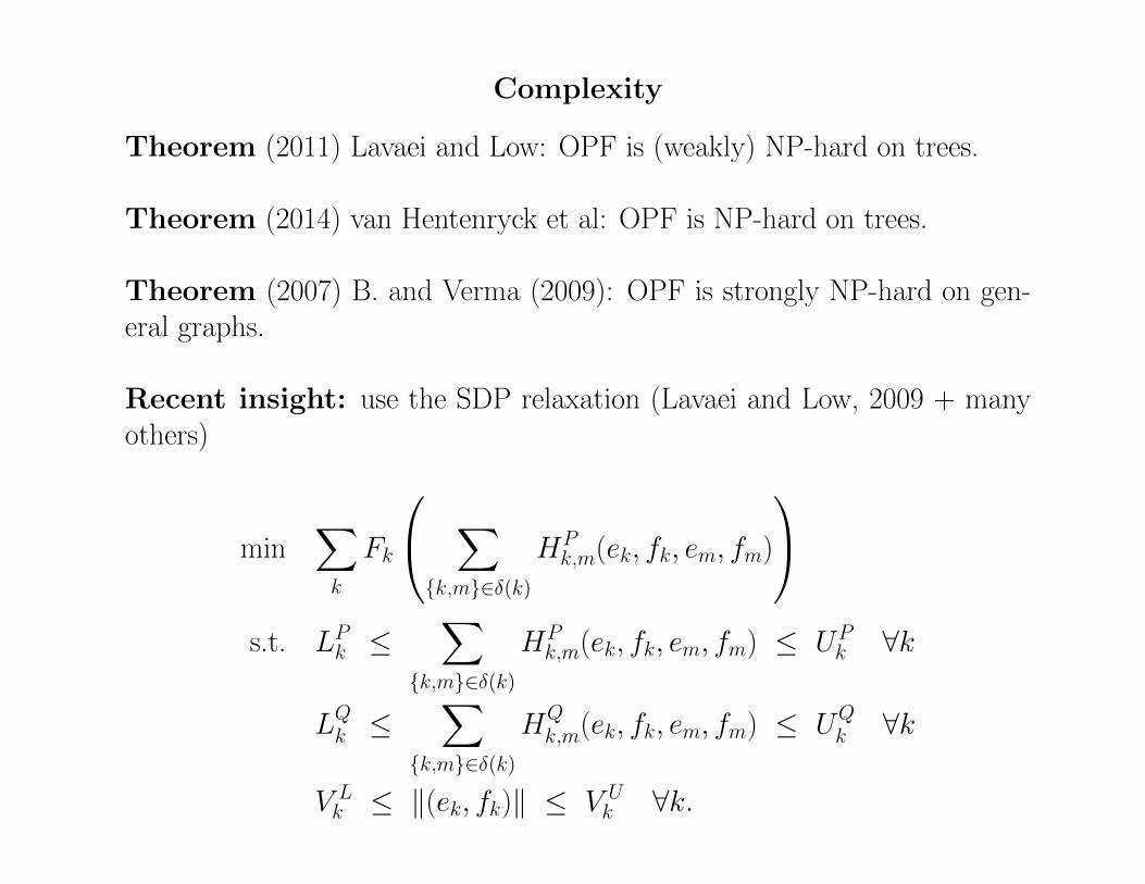
Complexity




Recent insight: use the SDP relaxation (Lavaei and Low, 2009 + manyothers)

min∑k

Fk

∑{k,m}∈δ(k)


s.t. LPk ≤

∑{k,m}∈δ(k)


k ∀k

LQk ≤∑

{k,m}∈δ(k)


k ∀k

V Lk ≤ ‖(ek, fk)‖ ≤ V U

k ∀k.

Complexity





Reformulation of ACOPF:

min F •Ws.t. Ai •W ≤ bi i = 1, 2, . . .

W � 0, W of rank 1.

Complexity





SDP Relaxation of OPF:

min F •Ws.t. Ai •W ≤ bi i = 1, 2, . . .

W � 0.

Complexity





SDP Relaxation of OPF:

min F •Ws.t. Ai •W ≤ bi i = 1, 2, . . .

W � 0.

Fact: The SDP relaxation is often good! (“near” rank 1 solution).

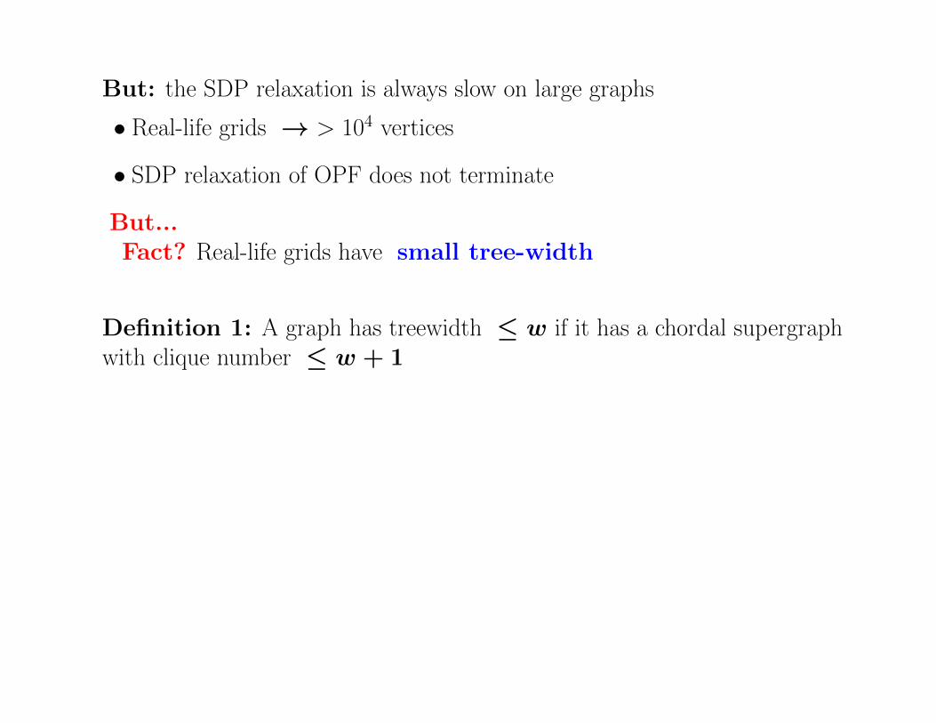
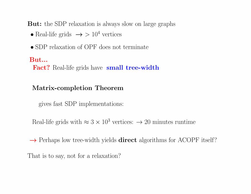
But: the SDP relaxation is always slow on large graphs

• Real-life grids → > 104 vertices

• SDP relaxation of OPF does not terminate

But...




But...Fact? Real-life grids have small tree-width

Definition 1: A graph has treewidth ≤ w if it has a chordal supergraphwith clique number ≤ w + 1





Definition 2: A graph has treewidth ≤ w if it is a subgraph of anintersection graph of subtrees of a tree, with ≤ w + 1 subtrees overlappingat any vertex





Definition 2: A graph has treewidth ≤ w if it is a subgraph of an inter-section graph of subtrees of a tree, with ≤ w + 1 subtrees overlapping atany vertex

(Seymour and Robertson, late 1980s)

Tree-width

Let G be an undirected graph with vertices V (G) and edges E(G).

A tree-decomposition of G is a pair (T,Q) where:

• T is a tree. Not a subtree of G, just a tree

• For each vertex t of T , Qt is a subset of V (G). These subsets satisfythe two properties:

(1) For each vertex v of G, the set {t ∈ V (T ) : v ∈ Qt} is a subtreeof T , denoted Tv.

(2) For each edge {u, v} of G, the two subtrees Tu and Tv intersect.

• The width of (T,Q) is maxt∈T |Qt| − 1.

1

2

3

4

5 6

→ two subtrees Tu, Tv may overlap even if {u, v} is not an edge of G

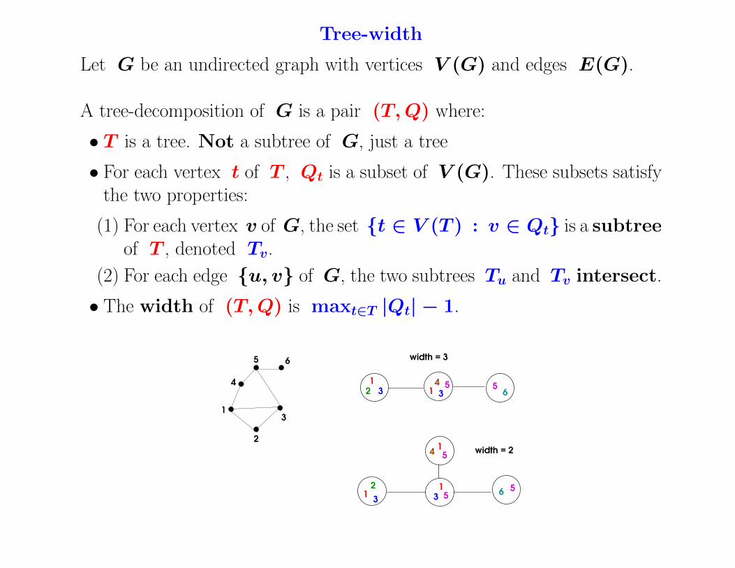
Tree-width

Let G be an undirected graph with vertices V (G) and edges E(G).

A tree-decomposition of G is a pair (T,Q) where:

• T is a tree. Not a subtree of G, just a tree

• For each vertex t of T , Qt is a subset of V (G). These subsets satisfythe two properties:

(1) For each vertex v of G, the set {t ∈ V (T ) : v ∈ Qt} is a subtreeof T , denoted Tv.

(2) For each edge {u, v} of G, the two subtrees Tu and Tv intersect.

• The width of (T,Q) is maxt∈T |Qt| − 1.

width = 3

width = 2

1

2

3

4

5 6

1

2 3 1 3

545

35

54

2 51

1

1 36

6





Matrix-completion Theorem

gives fast SDP implementations:

Real-life grids with ≈ 3× 103 vertices: → 20 minutes runtime





Matrix-completion Theorem

gives fast SDP implementations:

Real-life grids with ≈ 3× 103 vertices: → 20 minutes runtime

→ Perhaps low tree-width yields direct algorithms for ACOPF itself?

That is to say, not for a relaxation?

Much previous work using structured sparsity

• Bienstock and Ozbay

•Wainwright and Jordan

• Grimm, Netzer, Schweighofer

• Laurent

• Lasserre et al

•Waki, Kim, Kojima, Muramatsu

older work ...

• Lauritzen (1996): tree-junction theorem

• Bertele and Brioschi (1972): nonserial dynamic programming

• Bounded tree-width in combinatorial optimization (too many authors)

• Fulkerson and Gross (1965): matrices with consecutive ones

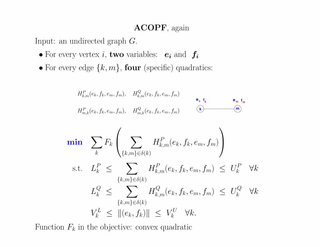
ACOPF, again





k,m(ek, fk, em, fm)



e efk k m mf

min∑k

Fk

∑{k,m}∈δ(k)


s.t. LPk ≤

∑{k,m}∈δ(k)


k ∀k

LQk ≤∑

{k,m}∈δ(k)


k ∀k

V Lk ≤ ‖(ek, fk)‖ ≤ V U

k ∀k.Function Fk in the objective: convex quadratic

ACOPF, again





k,m(ek, fk, em, fm)



e efk k m mf

min∑k

wk

s.t. LPk ≤∑

{k,m}∈δ(k)


k ∀k

LQk ≤∑

{k,m}∈δ(k)


k ∀k

V Lk ≤ ‖(ek, fk)‖ ≤ V U

k ∀k

wk = Fk

∑{k,m}∈δ(k)


∀k

Graphical QCQP


• For every vertex k, a set of variables: {xj : j ∈ I(k)}• For every edge e = {k,m}, a quadratic

He(x) = He ( {xj : j ∈ I(k) ∪ I(m)}) .

• For now, the sets I(k) are disjoint

min∑k

∑j∈I(k)

ck,jxj

s.t.∑e∈δ(k)

He(x) ≤ bk ∀k

0 ≤ xj ≤ 1, ∀j

→ Easy to solve if graph has small tree-width?

Subset-sum problem

Input: positive integers p1, p2, . . . , pn.

Problem: find a solution to:

n∑j=1

pjxj =1

2

n∑j=1

pj

xj ∈ {0, 1}, ∀j

(weakly) NP-hard (well...)

Subset-sum problem

Input: positive integers p1, p2, . . . , pn.

Problem: find a solution to:

n∑j=1

pjxj =1

2

n∑j=1

pj

xj(1− xj) = 0, ∀j

(weakly) NP-hard (well...)

This is a graphical QCQP on a star – so treewidth 1.

(Perhaps) approximate solutions?

{0, 1} solutions with error(

12

∑nj=1 pj

)ε in time polynomial in ε−1?

Graphical QCQP


• For every vertex k, a set of variables: {xj : j ∈ I(k)}• For every edge e = {k,m}, a quadratic

He(x) = He ( {xj : j ∈ I(k) ∪ I(m)}) .

• For now, the sets I(k) are disjoint

min cTx

s.t.∑e∈δ(k)

He(x) ≤ bk ∀k

0 ≤ xj ≤ 1, ∀j

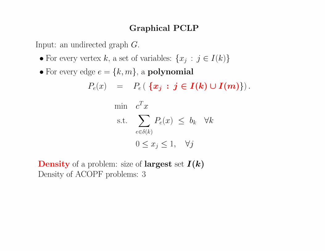
Graphical PCLP


• For every vertex k, a set of variables: {xj : j ∈ I(k)}• For every edge e = {k,m}, a polynomial

Pe(x) = Pe ( {xj : j ∈ I(k) ∪ I(m)}) .

min cTx

s.t.∑e∈δ(k)

Pe(x) ≤ bk ∀k

0 ≤ xj ≤ 1, ∀j

Density of a problem: size of largest set I(k)Density of ACOPF problems: 3

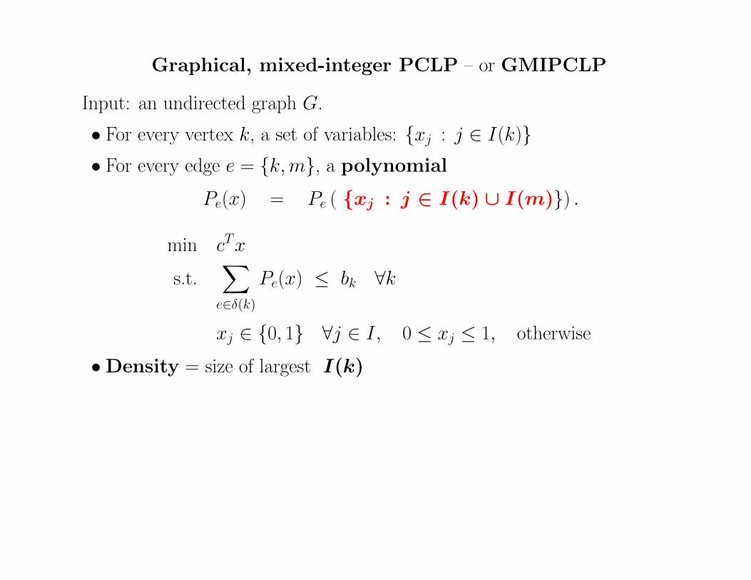
Graphical, mixed-integer PCLP – or GMIPCLP



Pe(x) = Pe ( {xj : j ∈ I(k) ∪ I(m)}) .

min cTx

s.t.∑e∈δ(k)

Pe(x) ≤ bk ∀k

xj ∈ {0, 1} ∀j ∈ I, 0 ≤ xj ≤ 1, otherwise

•Density = size of largest I(k)

Graphical, mixed-integer PCLP – or GMIPCLP



Pe(x) = Pe ( {xj : j ∈ I(k) ∪ I(m)}) .

min cTx

s.t.∑e∈δ(k)

Pe(x) ≤ bk ∀k


•Density = size of largest I(k)

Theorem 3

For any instance of GMIPCLP on a graph with treewidth w, densityd, max. degree π, and any fixed 0 < ε < 1, there is a linear programof size (rows + columns) O∗(πwdε−w n) whose feasibility and optimalityerror is O(ε)(abridged).

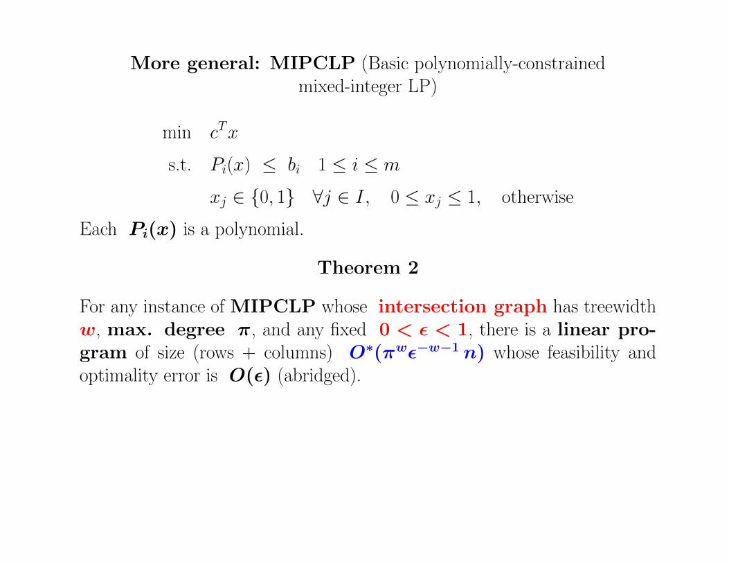
More general: MIPCLP (Basic polynomially-constrainedmixed-integer LP)

min cTx

s.t. Pi(x) ≤ bi 1 ≤ i ≤ m


Each Pi(x) is a polynomial.


min cTx

s.t. Pi(x) ≤ bi 1 ≤ i ≤ m



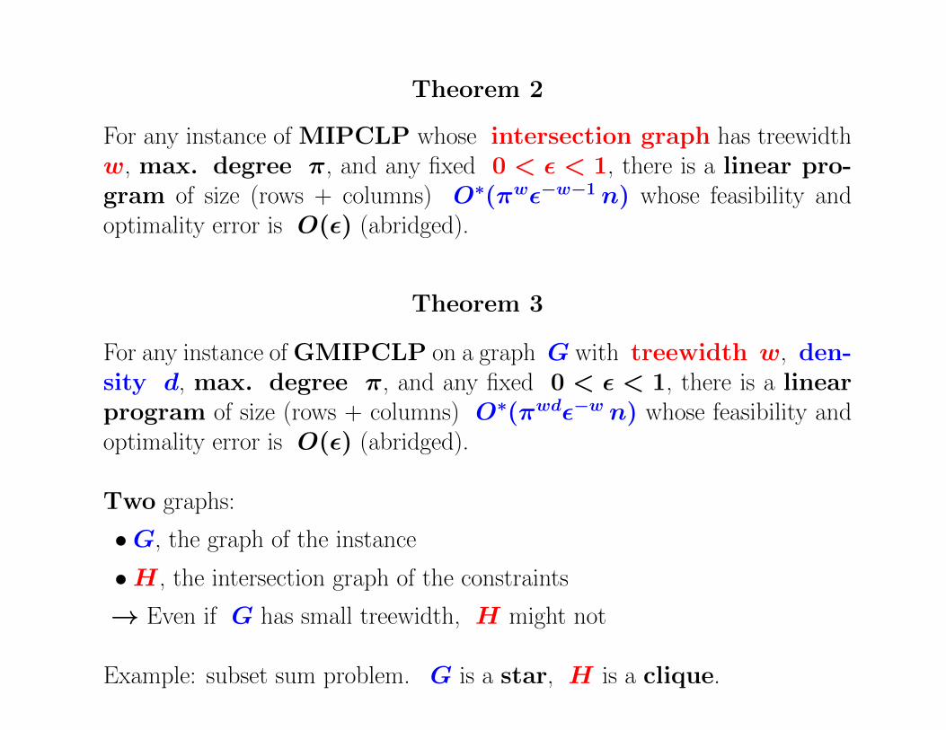
Theorem 2

For any instance of MIPCLP whose intersection graph has treewidthw, max. degree π, and any fixed 0 < ε < 1, there is a linear pro-gram of size (rows + columns) O∗(πwε−w−1 n) whose feasibility andoptimality error is O(ε) (abridged).


min cTx

s.t. Pi(x) ≤ bi 1 ≤ i ≤ m



Theorem 2


Intersection graph of a constraint system: (Fulkerson? (1962?))

• Has a vertex for every variably xj

• Has an edge {xi, xj} whenever xi and xj appear in the same constraint

Theorem 2


Theorem 3

For any instance of GMIPCLP on a graph G with treewidth w, den-sity d, max. degree π, and any fixed 0 < ε < 1, there is a linearprogram of size (rows + columns) O∗(πwdε−wd n) whose feasibility andoptimality error is O(ε) (abridged).

Theorem 2


Theorem 3

For any instance of GMIPCLP on a graph G with treewidth w, den-sity d, max. degree π, and any fixed 0 < ε < 1, there is a linearprogram of size (rows + columns) O∗(πwdε−w n) whose feasibility andoptimality error is O(ε) (abridged).

Two graphs:

•G, the graph of the instance

•H , the intersection graph of the constraints

→ Even if G has small treewidth, H might not

Example: subset sum problem. G is a star, H is a clique.

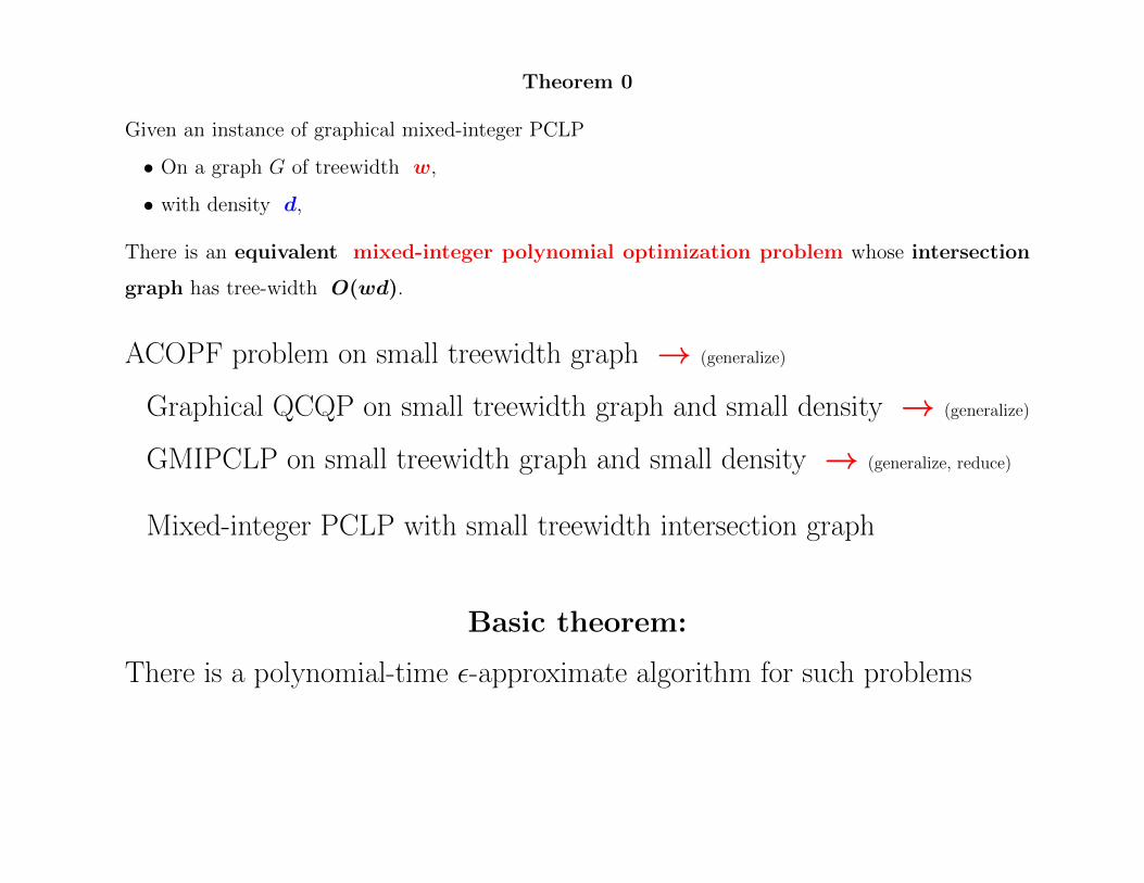
Theorem 0

Given an instance of graphical mixed-integer PCLP

• On a graph G of treewidth w,

• with density d,• For every vertex k, a set of variables: {xj : j ∈ I(k)}, for every edge e = {k,m}, a polynomial

Pe(x) = Pe ( {xj : j ∈ I(k) ∪ I(m)}) .

min cTx

s.t.∑e∈δ(k)

Pe(x) ≤ bk ∀k

xj ∈ {0, 1}, ∀j ∈ I, 0 ≤ xj ≤ 1, otherwise.

Density of a problem: size of largest set I(k)

There is an equivalent

mixed-integer polynomial optimization problem

whose intersection graph has tree-width O(wd).

Theorem 0

Given an instance of graphical mixed-integer PCLP

• On a graph G of treewidth w,

• with density d,

There is an equivalent mixed-integer polynomial optimization problem whose intersection

graph has tree-width O(wd).

ACOPF problem on small treewidth graph → (generalize)

Graphical QCQP on small treewidth graph and small density → (generalize)

GMIPCLP on small treewidth graph and small density → (generalize, reduce)

Mixed-integer PCLP with small treewidth intersection graph

Basic theorem:

There is a polynomial-time ε-approximate algorithm for such problems

Main technique: approximation through pure-binaryproblems

Glover, 1975 (abridged)

Let x be a variable, with bounds 0 ≤ x ≤ 1. Let 0 < γ < 1. Then wecan approximate

x ≈∑L

h=1 2−hyh

where each yh is a binary variable. In fact, choosing L = dlog2 ε−1e,

we have

x ≤∑L

h=1 2−hyh ≤ x+ ε.

→ Given a mixed-integer polynomially constrained LP (MIPCLP),apply this technique to each continuous variable xj

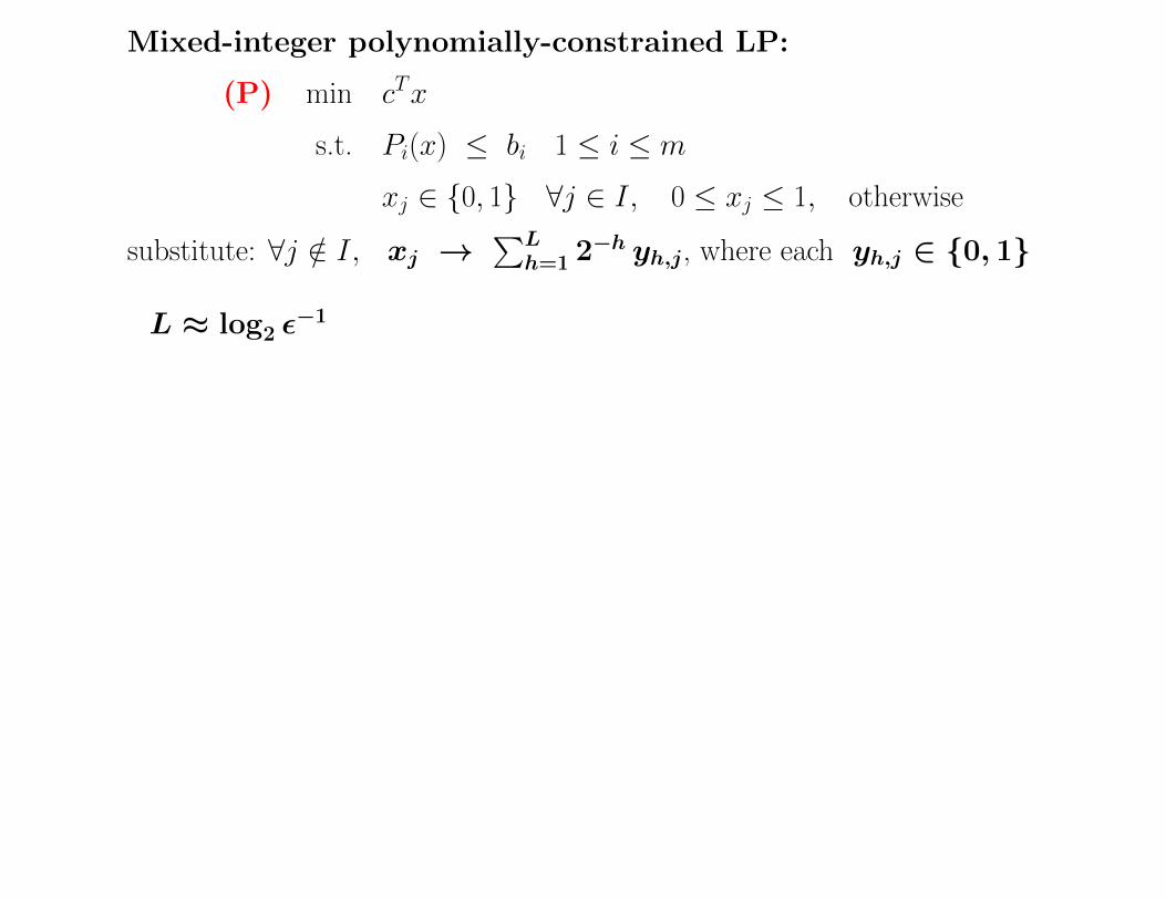
Mixed-integer polynomially-constrained LP:

(P) min cTx

s.t. Pi(x) ≤ bi 1 ≤ i ≤ m


substitute: ∀j /∈ I, xj →∑L

h=1 2−h yh,j, where each yh,j ∈ {0, 1}

L ≈ log2 ε−1


(P) min cTx

s.t. Pi(x) ≤ bi 1 ≤ i ≤ m




L ≈ log2 ε−1

obtain pure binary problem:

(Q) min cTz

s.t. Pi(z) ≤ bi 1 ≤ i ≤ m

zk ∈ {0, 1} ∀kIf (P) has intersection graph of treewidth w,

then (Q) has intersection graph of treewidth Lw.


(P) min cTx

s.t. Pi(x) ≤ bi 1 ≤ i ≤ m




L ≈ log2 ε−1

obtain pure binary problem:

(Q) min cTz

s.t. Pi(z) ≤ bi 1 ≤ i ≤ m

zk ∈ {0, 1} ∀kIf (P) has intersection graph of treewidth w,

then (Q) has intersection graph of treewidth Lw.

Theorem

Consider a pure-binary PCLP with n variables.If the intersection graph has treewidth ≤W then there is an exact linearprogramming formulation with

O(2Wn) variables and constraints.

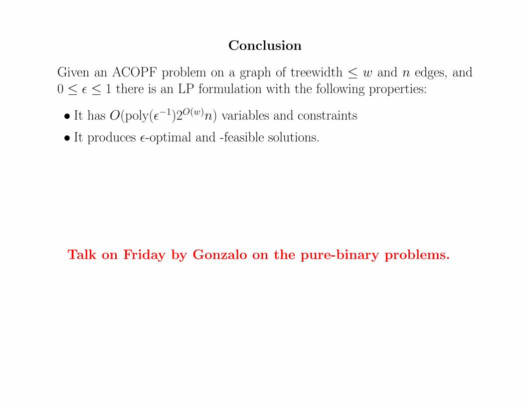
Conclusion

Given an ACOPF problem on a graph of treewidth ≤ w and n edges, and0 ≤ ε ≤ 1 there is an LP formulation with the following properties:

• It has O(poly(ε−1)2O(w)n) variables and constraints

• It produces ε-optimal and -feasible solutions.

Talk on Friday by Gonzalo on the pure-binary problems.

Date post:	08-May-2018
Category:	Documents
Upload:	lexuyen
View:	229 times
Download:	0 times

LP formulations for mixed-integer polynomial …dano/talks/ismp15.pdf · LP formulations for...

Documents