LP. Lecture 6: Ch. 6: the simplex method in matrix form,and Section 7.1: sensitivity analysis

I matrix notationI simplex algorithm in matrix notationI exampleI negative transpose property: proofI sensitivity analysis (section 7.1)

1 / 27

Matrix notation

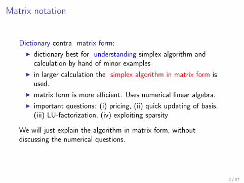
Dictionary contra matrix form:I dictionary best for understanding simplex algorithm and

calculation by hand of minor examplesI in larger calculation the simplex algorithm in matrix form is

used.I matrix form is more efficient. Uses numerical linear algebra.I important questions: (i) pricing, (ii) quick updating of basis,

(iii) LU-factorization, (iv) exploiting sparsity

We will just explain the algorithm in matrix form, withoutdiscussing the numerical questions.

2 / 27

Consider LP problem in standard form

max∑n

j=1 cjxj

s.t. ∑nj=1 ai ,jxj ≤ bi for i = 1, . . . ,m

xj ≥ 0 for j = 1, . . . , n.

Converting to equations by using slack variables.

xn+i = bi −∑n

j=1 ai ,jxj for i = 1, . . . ,m.

Matrix form:max cT xs.t.

Ax = b,x ≥ O

where

3 / 27

A =

a11 . . . a1n 1 0 . . . 0a21 . . . a2n 0 1 . . . 0

......

. . .

am1 . . . amn 0 0 1

, b =

b1

b2

...bm

,

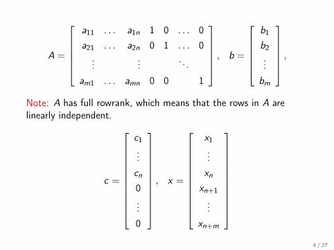
Note: A has full rowrank, which means that the rows in A arelinearly independent.

c =

c1

...cn

0...0

, x =

x1

...xn

xn+1

...xn+m

4 / 27

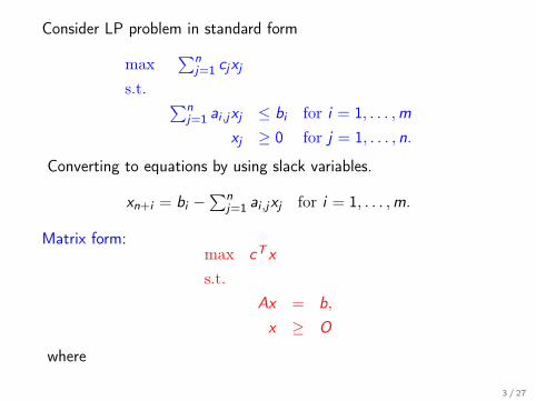
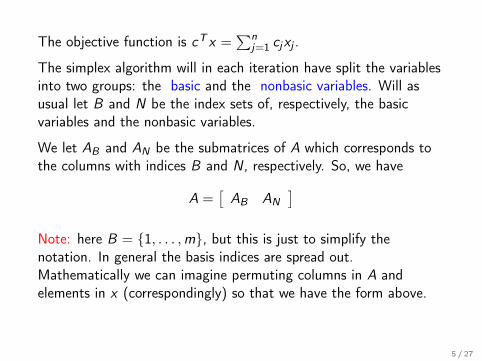
The objective function is cT x =∑n

j=1 cjxj .

The simplex algorithm will in each iteration have split the variablesinto two groups: the basic and the nonbasic variables. Will asusual let B and N be the index sets of, respectively, the basicvariables and the nonbasic variables.

We let AB and AN be the submatrices of A which corresponds tothe columns with indices B and N, respectively. So, we have

A =[

AB AN]

Note: here B = {1, . . . ,m}, but this is just to simplify thenotation. In general the basis indices are spread out.Mathematically we can imagine permuting columns in A andelements in x (correspondingly) so that we have the form above.

5 / 27

Primal simplex algorithmSplit x and c similarly as

x =

[xB

xN

], c =

[cB

cN

]

With that

Ax =[

AB AN] [ xB

xN

]= AB xB + AN xN ,

cT x =[

cTB cT

N] [ xB

xN

]= cT

B xB + cTN xN .

The set of equations Ax = b is now

ABxB + ANxN = b

6 / 27

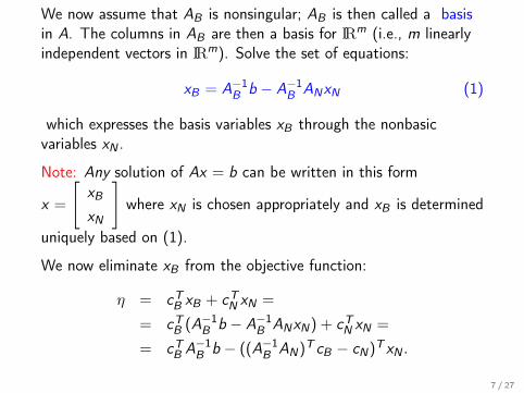
We now assume that AB is nonsingular; AB is then called a basisin A. The columns in AB are then a basis for IRm (i.e., m linearlyindependent vectors in IRm). Solve the set of equations:

xB = A−1B b − A−1

B ANxN (1)

which expresses the basis variables xB through the nonbasicvariables xN .

Note: Any solution of Ax = b can be written in this form

x =

[xB

xN

]where xN is chosen appropriately and xB is determined

uniquely based on (1).

We now eliminate xB from the objective function:

η = cTB xB + cT

N xN =

= cTB (A−1

B b − A−1B ANxN) + cT

N xN =

= cTB A−1

B b − ((A−1B AN)T cB − cN)T xN .

7 / 27

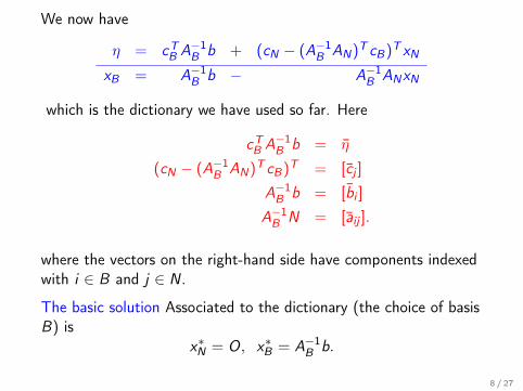
We now have

η = cTB A−1

B b + (cN − (A−1B AN)T cB)T xN

xB = A−1B b − A−1

B ANxN

which is the dictionary we have used so far. Here

cTB A−1

B b = η

(cN − (A−1B AN)T cB)T = [cj ]

A−1B b = [bi ]

A−1B N = [aij ].

where the vectors on the right-hand side have components indexedwith i ∈ B and j ∈ N.

The basic solution Associated to the dictionary (the choice of basisB) is

x∗N = O, x∗B = A−1B b.

8 / 27

Will now look at the dual. Recall the correspondenceI the primal variable xj corresponds to the dual slack variable zj

I the primal slack variable wi corresponds to the dual slackvariable yi

We say that xj and zj are complementary, and that wi and yi arecomplementary. Complementary variables have opposite roles in theequations: they are on the opposite sides.

This means that: a variable is in basis if and only if thecomplementary variable is out of basis.

9 / 27

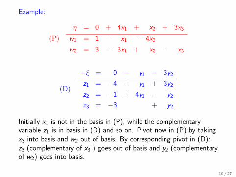
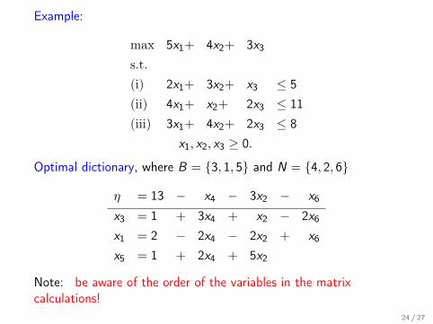
Example:

(P)η = 0 + 4x1 + x2 + 3x3

w1 = 1 − x1 − 4x2

w2 = 3 − 3x1 + x2 − x3

(D)

−ξ = 0 − y1 − 3y2

z1 = −4 + y1 + 3y2

z2 = −1 + 4y1 − y2

z3 = −3 + y2

Initially x1 is not in the basis in (P), while the complementaryvariable z1 is in basis in (D) and so on. Pivot now in (P) by takingx3 into basis and w2 out of basis. By corresponding pivot in (D):z3 (complementary of x3 ) goes out of basis and y2 (complementaryof w2) goes into basis.

10 / 27

In each pivot in (P) one basic variable and one nonbasic variableswitch roles. By a corresponding pivot in (D) the complementaryvariables in (D) will also switch roles, but the opposite way.

This means that complementary variables still have opposite roleswhen it comes to being in basis. Because of this complementaryproperty we choose to arrange the variables in the two problems likethis:

(x1, . . . , xn,w1, . . . ,wm) → (x1, . . . , xn, xn+1, . . . , xn+m)

(z1, . . . , zn, y1, . . . , ym) → (z1, . . . , zn, zn+1, . . . , zn+m)

So then xj and zj are complementary for j = 1, . . . , n + m. Inparticular, the basic variables in (D) be zN (not zB !).

11 / 27

Because of the negative transpose property the dual dictionary(with basis B) is given by:

−ξ = −cTB A−1

B b − (A−1B b)T zB

zN = (A−1B AN)T cB − cN + (A−1

B AN)T zB .

The corresponding dual basic solution for this dictionary is

z∗B = O, z∗N = (A−1B AN)T cB − cN .

We now introduceη∗ = cT

B A−1B b

which is the value of the objective function η in (P) for the basissolution associated to B .

12 / 27

Conclusion: primal and dual dictionary for basis B now becomes

η = η∗ − (z∗N)T xN

xB = x∗B − A−1B ANxN

(2)

−ξ = −η∗ − (x∗B)T zB

zN = z∗N + (A−1B AN)T zB

(3)

Note the negative transpose property.

13 / 27

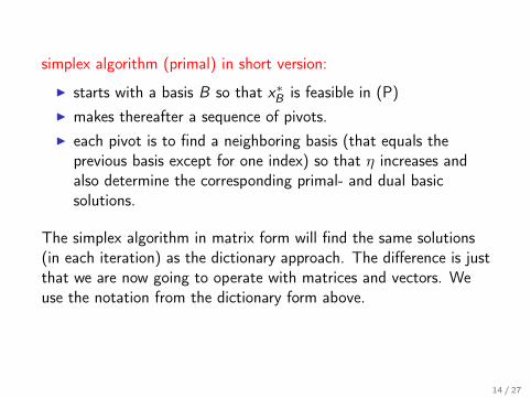
simplex algorithm (primal) in short version:

I starts with a basis B so that x∗B is feasible in (P)I makes thereafter a sequence of pivots.I each pivot is to find a neighboring basis (that equals the

previous basis except for one index) so that η increases andalso determine the corresponding primal- and dual basicsolutions.

The simplex algorithm in matrix form will find the same solutions(in each iteration) as the dictionary approach. The difference is justthat we are now going to operate with matrices and vectors. Weuse the notation from the dictionary form above.

14 / 27

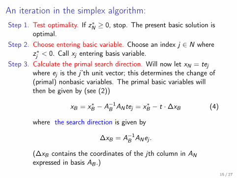
An iteration in the simplex algorithm:Step 1. Test optimality. If z∗N ≥ 0, stop. The present basic solution is

optimal.Step 2. Choose entering basic variable. Choose an index j ∈ N where

z∗j < 0. Call xj entering basis variable.Step 3. Calculate the primal search direction. Will now let xN = tej

where ej is the j ’th unit vector; this determines the change of(primal) nonbasic variables. The primal basic variables willthen be given by (see (2))

xB = x∗B − A−1B ANtej = x∗B − t ·∆xB (4)

where the search direction is given by

∆xB = A−1B ANej .

(∆xB contains the coordinates of the jth column in ANexpressed in basis AB .)

15 / 27

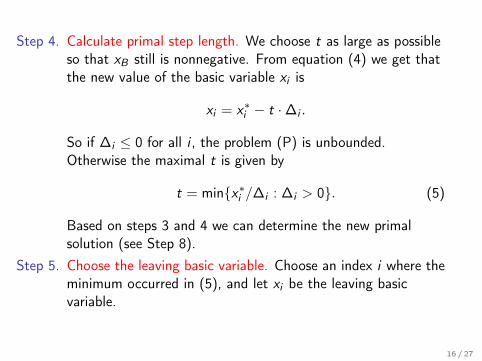
Step 4. Calculate primal step length. We choose t as large as possibleso that xB still is nonnegative. From equation (4) we get thatthe new value of the basic variable xi is

xi = x∗i − t ·∆i .

So if ∆i ≤ 0 for all i , the problem (P) is unbounded.Otherwise the maximal t is given by

t = min{x∗i /∆i : ∆i > 0}. (5)

Based on steps 3 and 4 we can determine the new primalsolution (see Step 8).

Step 5. Choose the leaving basic variable. Choose an index i where theminimum occurred in (5), and let xi be the leaving basicvariable.

16 / 27

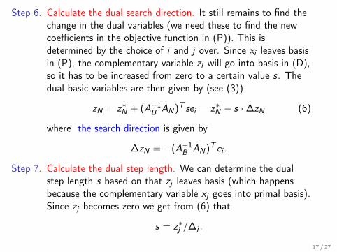
Step 6. Calculate the dual search direction. It still remains to find thechange in the dual variables (we need these to find the newcoefficients in the objective function in (P)). This isdetermined by the choice of i and j over. Since xi leaves basisin (P), the complementary variable zi will go into basis in (D),so it has to be increased from zero to a certain value s. Thedual basic variables are then given by (see (3))

zN = z∗N + (A−1B AN)T sei = z∗N − s ·∆zN (6)

where the search direction is given by

∆zN = −(A−1B AN)T ei .

Step 7. Calculate the dual step length. We can determine the dualstep length s based on that zj leaves basis (which happensbecause the complementary variable xj goes into primal basis).Since zj becomes zero we get from (6) that

s = z∗j /∆j .

17 / 27

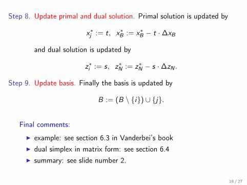
Step 8. Update primal and dual solution. Primal solution is updated by

x∗j := t, x∗B := x∗B − t ·∆xB

and dual solution is updated by

z∗i := s, z∗N := z∗N − s ·∆zN .

Step 9. Update basis. Finally the basis is updated by

B := (B \ {i}) ∪ {j}.

Final comments:

I example: see section 6.3 in Vanderbei’s bookI dual simplex in matrix form: see section 6.4I summary: see slide number 2.

18 / 27

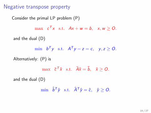
Negative transpose property

Consider the primal LP problem (P)

max cT x s.t. Ax + w = b, x ,w ≥ O.

and the dual (D)

min bT y s.t. AT y − z = c , y , z ≥ O.

Alternatively: (P) is

max cT x s.t. Ax = b, x ≥ O.

and the dual (D)

min bT y s.t. AT y = c , y ≥ O.

19 / 27

Here

A =[

A I], c =

[cO

], x =

[xw

],

and

A =[−I AT ]

, b =

[Ob

], y =

[zy

],

Complementary - primal and dual basis: column j is in basis in A ifand only if column j is not in basis in A.

In the beginning the m last columns in A are in basis, and the nfirst columns in A are in basis.

After a few pivots

A =[

A I]

=[

AN AB]P

for a permutation matrix P . The columns in A are permuted. Sincethe corresponding pivots occur in the dual

20 / 27

A =[−I AT ]

=[

AB AN]P

But P−1 = PT , so PPT = I . Which means that

AAT =[

AN AB]PPT

[AT

BAT

N

]= AN AT

B + AB ATN

and in addition we have that

AAT =[

A I] [ −I

A

]= −A + A = O.

So:AN AT

B + AB ATN = O

By some algebra we get that

A−1B AN = −(A−1

B AN)T

This shows the negative transpose property.21 / 27

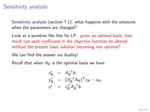
Sensitivity analysis

Sensitivity analysis (section 7.1): what happens with the solutionswhen the parameters are changed?

Look at a question like this for LP: given an optimal basis, howmuch can each coefficient in the objective function be alteredwithout the present basic solution becoming non optimal?

We can find the answer via duality!

Recall that when AB is the optimal basis we have

x∗B = A−1B b,

y∗N = (A−1B AN)T cB − cN ,

η∗ = cTB A−1

B b.

22 / 27

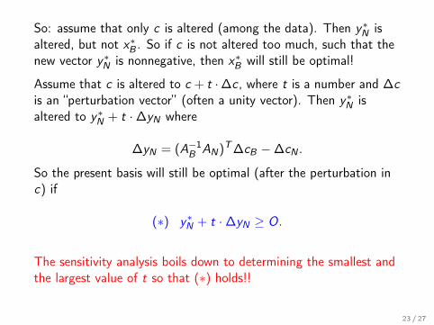
So: assume that only c is altered (among the data). Then y∗N isaltered, but not x∗B . So if c is not altered too much, such that thenew vector y∗N is nonnegative, then x∗B will still be optimal!

Assume that c is altered to c + t ·∆c , where t is a number and ∆cis an “perturbation vector” (often a unity vector). Then y∗N isaltered to y∗N + t ·∆yN where

∆yN = (A−1B AN)T ∆cB −∆cN .

So the present basis will still be optimal (after the perturbation inc) if

(∗) y∗N + t ·∆yN ≥ O.

The sensitivity analysis boils down to determining the smallest andthe largest value of t so that (∗) holds!!

23 / 27

Example:

max 5x1+ 4x2+ 3x3

s.t.(i) 2x1+ 3x2+ x3 ≤ 5(ii) 4x1+ x2+ 2x3 ≤ 11(iii) 3x1+ 4x2+ 2x3 ≤ 8

x1, x2, x3 ≥ 0.

Optimal dictionary, where B = {3, 1, 5} and N = {4, 2, 6}

η = 13 − x4 − 3x2 − x6

x3 = 1 + 3x4 + x2 − 2x6

x1 = 2 − 2x4 − 2x2 + x6

x5 = 1 + 2x4 + 5x2

Note: be aware of the order of the variables in the matrixcalculations!

24 / 27

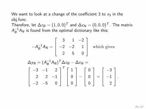
We want to look at a change of the coefficient 3 to x3 in theobj.func.Therefore, let ∆cB = (1, 0, 0)T and ∆cN = (0, 0, 0)T . The matrixA−1

B AN is found from the optimal dictionary like this:

−A−1B AN =

3 1 −2−2 −2 12 5 0

which gives

∆yN = (A−1B AN)T ∆cB −∆cN = −3 −1 2

2 2 −1−2 −5 0

T 1

00

− 0

00

=

−3−12

.

25 / 27

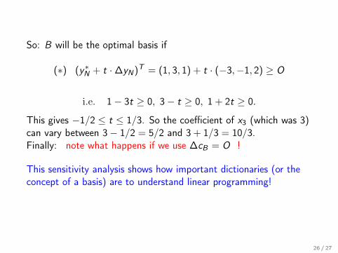
So: B will be the optimal basis if

(∗) (y∗N + t ·∆yN)T = (1, 3, 1) + t · (−3,−1, 2) ≥ O

i.e. 1− 3t ≥ 0, 3− t ≥ 0, 1 + 2t ≥ 0.

This gives −1/2 ≤ t ≤ 1/3. So the coefficient of x3 (which was 3)can vary between 3− 1/2 = 5/2 and 3 + 1/3 = 10/3.Finally: note what happens if we use ∆cB = O !

This sensitivity analysis shows how important dictionaries (or theconcept of a basis) are to understand linear programming!

26 / 27

Further themes are:

I some game theoryI convexity (geometrical aspects of LP), andI network flow problems.

27 / 27