Received 11 July 2007, in final form 7 November 2007Published 28 January 2008Online at stacks.iop.org/RoPP/71/026001
AbstractExperimental progress in the miniaturization of electronic devices has made routinely available in thelaboratory small electronic systems, on the micrometre or sub-micrometre scale, which at lowtemperature are sufficiently well isolated from their environment to be considered as fully coherent.Some of their most important properties are dominated by the interaction between electrons.Understanding their behaviour therefore requires a description of the interplay between interferenceeffects and interactions.
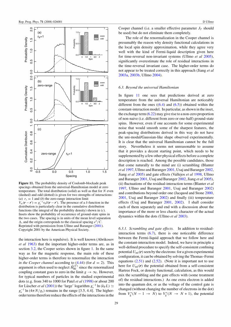
The goal of this review is to address this relatively broad issue and more specifically to address itfrom the perspective of the quantum chaos community. I will therefore present some of the conceptsdeveloped in the field of quantum chaos which may be applied to the study of many-body effects inmesoscopic and nanoscopic systems. Their implementation is illustrated in a few examples ofexperimental relevance such as persistent currents, mesoscopic fluctuations of Kondo properties orCoulomb blockade. I will furthermore try to bring out, from the various physical illustrations, some ofthe specific advantages on more general grounds of the quantum chaos based approach.
(Some figures in this article are in colour only in the electronic version)
This article was invited by Professor S Washburn.
Contents
1. Introduction 22. Basic tools 3
2.1. Semiclassical formalism 32.2. Random-matrix and random-plane-wave
models in the hard-chaos regime 62.3. Screening of the Coulomb interaction in quan-
tum dots 83. Orbital magnetism: general formalism 9
3.1. First order perturbations 103.2. Correlations effects 11
4. Orbital magnetism: diffusive and ballistic systems 134.1. Diffusive systems 134.2. Ballistic systems 174.3. Discussion 19
The title of this review may seem self-contradictory in tworespects. To begin with, it associates chaos, a purely classicalnotion, with quantum physics. Furthermore it implies that thisassociation, which as we will see refers traditionally to thestudy of low-dimensional non-interacting quantum systems,will be considered in the context of many-body physics.
The first of these contradictions is however mainly aquestion of semantics. Indeed, if in an early period ofdevelopment of the field of quantum chaos, some of the issuesaddressed had to do with the possible existence of true chaoticdynamics for quantum systems, this was relatively quicklyanswered, essentially in the negative. Quantum chaos nowmainly refers to the study of the consequences, for a quantumsystem, of the more or less chaotic nature of the dynamics of itsclassical analogue. It has followed two main avenues. The firstone is based on semiclassical techniques—specifically the useof semiclassical Green’s functions in the spirit of Gutzwiller’strace formulae (Gutzwiller 1971, 1990, 1991, Balian and Bloch1972, Berry and Tabor 1977)—which provides a link between aquantum system and its h → 0 limit. The second is associatedwith the Bohigas Giannoni Schmit conjecture (Bohigas et al1984a, 1984b, Bohigas 1991) or related approaches Peres(1984), which states that the spectral fluctuations of classicallychaotic systems can be described using the proper ensemblesof random matrices.
Some of the beauty of quantum chaos is that it hasdeveloped a set of tools which have found applicationsin a large variety of different physical contexts, rangingfrom molecular and atomic physics (Delande and Gay 1986,Wintgen and Friedrich 1986, Wintgen 1987, Delande et al1991) to acoustics (Derode et al 1995, Fink 1997, Fink et al2000), nuclear physics (Bohigas and Leboeuf 2002, Olofssonet al 2006), cold atoms (Mouchet et al 2001, Hensinger et al2001, Steck et al 2001, 2002), optical (Nockel and Stone 1997,Gmachl et al 1998) or microwave (Stockmann and Stein 1990,Sridhar 1991, Alt et al 1995, Kudrolli et al 1995, Pradhan andSridhar 2000) resonators and of course mesoscopic physics(Richter et al 1996b, Richter 2000, Alhassid 2000). With fewexceptions (see nevertheless Bohigas and Leboeuf (2002) andOlofsson et al (2006)) most of these physical systems sharethe property of being correctly described by non-interacting,low-dimensional, models.
This is true in spite of the fact that random-matrixensembles were introduced in the early fifties by Wigner (seethe series of papers reprinted in Porter (1965)) to explainthe statistics of slow neutron resonances and were thereforeapplied in the context of strongly interacting systems. In thatcase however, it was less the notion of chaos than the one ofcomplexity (large number of degrees of freedom, strong andcomplicated interactions) which was proposed by Wigner tojustify this approach.
At any rate, the scope of this review will be concernedwith a very different type of interacting system, namely,the Landau–Fermi liquid, for which the system can beexplained as a set of quasi-particles interacting weaklythrough a (renormalized) interaction amenable to perturbative
treatment. More specifically, what we have in mind arevarious realizations of fully coherent, confined electron gasses,with a density high enough that a Landau–Fermi-liquidtype description applies. These are typically semiconductorquantum dots or small metallic nano-particles, within whicha few tens to a few thousands of electrons interact through ascreened Coulomb interaction.
Although this screened interaction between electrons isweak and is therefore well described by a standard perturbativeapproach (first order perturbation in the simplest cases oreventually with some re-summation of higher-order termsin other situations), some important physical processes areactually largely dominated by them. Moreover, the systemsconsidered are only weakly affected by their environment andcan therefore be assumed to be fully coherent. Because ofthe confinement, translational invariance is then broken, andsome new and interesting physics is brought in by the factthat, in the non-interacting limit from which the perturbationscheme is developed, eigenstates are not just plane waves.The mesoscopic fluctuations associated with confinement andinterference need to be taken into account for the eigenstatesand one-particle energies, either at a statistical level or in adetailed way associated with a given geometry.
Describing these mesoscopic fluctuations and implement-ing their consequences for many-body effects can be done ina variety of ways. For diffusive systems, techniques based ondiagrammatic perturbation expansion in the disorder potentialcan be used (Altshuler and Aronov 1985, Aleiner et al 2002,Akkermans and Montambaux 2007), as well as approachesbased on the super-symmetric σ -model (Efetov 1999, Mirlin2000), which is also appropriate for the description of ballis-tic chaotic systems (Blanter et al 2001a) (see also Andreevet al (1996), Leyvraz and Seligman (1997) and Agam et al(1997) in this context). In this review, I shall however limitmyself to the methods coming from the quantum chaos com-munity. One reason for this limitation of scope is that thereare already very good and complete reviews which give an ex-cellent account of the other approaches. Another is that thequantum chaos perspective is in many useful cases more intu-itive and somewhat simpler to apply from a technical point ofview. As a consequence, this will make it possible to present inan essentially self-contained way the technical tools requiredto understand a large class of many-body effects relevant forthese quantum dots or nano-particles, as long as they are inthe Landau–Fermi-liquid regime. The goal is that it shouldbe possible to follow almost all of the review with a graduatelevel in quantum mechanics and, in some cases, basic notionsof many-body theory such as can be found in classic textbookssuch as Fetter and Walecka (1971). This, I hope, will makeit particularly convenient for experimentalists or theoreticianswho wish to enter into this field.
Another advantage of the quantum chaos based approachis that it is by nature more flexible and is therefore not limitedto chaotic or diffusive dynamics. How much physics is missedby other points of view because of this limitation can bedebated, and I will return to this discussion at the end of thisreview. However, if for metallic nano-particles the choice ofa description in terms of a disordered (diffusive) system is
2
Rep. Prog. Phys. 71 (2008) 026001 D Ullmo
dictated by the actual physics of these materials, it is clearthat for semiconductor quantum dots, one reason as to why somuch focus has been put on chaotic dynamics is that it is theonly description that could be addressed by the more traditionaltechniques of solid state physics. Having a tool which makesit possible to consider other kinds of dynamics at least givesthe possibility of asking the question of whether anything new,or interesting, can be found in these other regimes.
The structure of this review is therefore the following.The first section is devoted to the description of the basictools necessary to study the physical problems we want toconsider. As we want to address different energy scales,or from an experimental point of view different temperatureranges, it will be necessary to introduce a few complementarypoint of views. Semiclassical techniques, and in particular theuse of semiclassical Green’s function, will be well adaptedto temperature ranges significantly larger than the mean levelspacing �. They are the subject of section 2.1. The low(T < �) temperature regime however requires a modelling ofindividual energies and wave-functions and are therefore betterdescribed, in the hard-chaos regime, by statistical approachessuch as random-matrix theory and the random plane-wavemodel. The latter is introduced in section 2.2. Finallysection 2.3 provides a discussion of the screening of theCoulomb interaction.
I then turn to the description of a few examples of physicalsystems where the physics is dominated by the interplay ofinteraction effects and mesoscopic fluctuations. The choice ofthese examples is of course quite arbitrary, and the criterionfor selecting them is essentially my familiarity with the issue.Therefore, there will be a strong bias towards questions Ihave actually worked on, which should not be interpreted asa statement about their relative importance. I start with adiscussion of the orbital magnetic response with some generalconsiderations in section 3 followed by a few specific examplesof diffusive and ballistic systems in section 4. One importantdifficulty to be addressed here is the renormalization of theinteraction due to higher-order terms in the Cooper channel,and this issue will be discussed in detail in both the diffusiveand ballistic regimes. In section 5, I wander briefly away fromFermi-liquid systems and address the mesoscopic fluctuationsassociated with the physics of a Kondo impurity (Kondo1964, Hewson 1993) placed in a finite size system. The lastphysical example is, in section 6, the role of interactions in thefluctuation of peak spacing in Coulomb blockade (Beenakker1991, Grabert and Devoret 1992, Weinmann et al 1996, Sohnet al 1997) experiments. After a general introduction of theuniversal-Hamiltonian picture, I cover the various physicaleffects which need to be further considered if one expects tounderstand experimental peak spacing and ground-state spindistributions for these systems.
Finally, the concluding section contains some generaldiscussion and in particular comes back to the issue of non-chaotic dynamics.
2. Basic tools
2.1. Semiclassical formalism
Consider a system of indistinguishable Fermions governed bythe one-particle Hamiltonian
H1p = − h2
2me� + U(r) (2.1)
and interacting weakly through the two-body potentialV (r − r′). A systematic perturbative expansion can beconstructed to arbitrary order (if necessary) in terms of theunperturbed Green’s function1
G(r, r′; ε)def= 〈r| 1
ε − H1p|r′〉 =
∑κ
ϕκ(r)ϕ∗κ (r
′)ε − εκ
, (2.2)
where in the last expression εκ and ϕκ are, respectively, theenergies and eigenstates of H1p. In a clean bulk systemU(r) ≡ 0 so that the eigenstates are just plane waves andthe expression of Green’s function becomes trivial in themomentum representation. For confined (coherent) systemshowever, translational invariance is lost and there is ingeneral no simple expression for the exact eigenstates andeigenfunctions. It therefore becomes necessary to find someapproximation scheme for the unperturbed Green’s functionitself before considering a perturbation expansion in theinteraction.
2.1.1. Semiclassical Green’s function. In many regimes ofinterest a semiclassical approach can be used to fulfil this role.This includes the case where the confining potential U(r) isa smooth function on the scale of the Fermi wavelength λF,but also, for instance, when it contains a weak, eventuallyshort range, disorder, as long as λF is much smaller than theelastic mean free path �. Under these conditions, the retarded
Green’s function GR(ε)def= limη→0 G(ε + iη) can be written as
a sum over all classical trajectories j joining r′ to r at energyε (Gutzwiller 1990, 1991):
GR(r, r′; ε) �∑
j :r′→r
GRj (r, r′; ε),
GRj (r, r′; ε)
def= 2π
(2iπh)(d+1)/2Dj(ε)
× exp(iSj (ε)/h − iζjπ/2), (2.3)
with d the number of degrees of freedom,
Sj (ε) =∫ r
r′p · dr (2.4)
the classical action along the trajectory j and
Dj(ε) =∣∣∣∣ 1
r1r′1
det′[− ∂2S
∂r∂r′
]∣∣∣∣1/2
(2.5)
1 All Green’s functions used in this review will be unperturbed Green’sfunctions. I shall therefore not use any subscript to distinguish them fromthe interacting ones.
3
Rep. Prog. Phys. 71 (2008) 026001 D Ullmo
a determinant describing the stability of trajectories near j .In (2.5) r = (r1, . . . , rd), and the prime on the determinantindicates that the first component (i.e. first row ∂2S/∂r1∂r ′
i
and first column ∂2S/∂ri∂r ′1, i = 1, · · · , d) is omitted. Finally,
the Maslov index ζj essentially counts the number of caustics(i.e. places where the determinant Dj is zero) on the trajectoryj between r′ and r.2 For two-dimensional systems (d = 2),the determinant takes the particularly simple form
Dj(ε) =∣∣∣∣∣ 1
r‖r ′‖
1(∂r⊥/∂p′
⊥)r⊥
∣∣∣∣∣1/2
, (2.6)
where r‖ and r⊥ are the r-components, respectively, paralleland orthogonal to the trajectory.
2.1.2. Simple properties of the classical action. Manyimportant characteristic features of the semiclassical Green’sfunction, and therefore of the fermion gas, can be directlydeduced from basic properties of classical action (Goldstein1964, Arnold 1989). In particular:
(i) the variation with respect to the energy:
∂Sj
∂ε= tj , (2.7)
where tj is the time elapsed to go from r′ to r alongtrajectory j at energy ε;
(ii) the variation with respect to the position:
∂Sj
∂r′ = −p′j
∂Sj
∂r= pj ; (2.8)
and finally(iii) the effect of a perturbation. Indeed, let us assume that the
one-particle Hamiltonian can be written as the sum of amain term H0 and a small perturbation H1:
H1p = H0 + H1, (2.9)
and let us denote by S0j the action calculated for the
trajectory j , i.e. (r0j (t), p0(t))j , t ∈ [0, t0], joining r′
to r under the Hamiltonian H0. We then have
δSjdef= Sj − S0
j � −∫ t0
0dtH1(r0
j (t), p0j (t)). (2.10)
Note there is no need for H1 to be small on the quantum scale,and therefore (2.10) remains applicable much beyond the limitof quantum perturbation theory3.
To illustrate how the above properties can be used in ourcontext, let us consider for instance the (unperturbed) localdensity of states,
νloc(r; ε)def=
∑κ
|ϕκ(r)|2δ(ε − εκ) = − 1
πImGR(r, r; ε).
(2.11)2 For the kind of kinetic plus potential Hamiltonian we consider here, theMaslov index increases by one at each crossing of a caustic. Note howeverthat for a more general Hamiltonian it may however also decrease.3 It should be stressed that the exponential sensitivity to perturbations ofchaotic trajectories does not prevent finding a perturbed trajectory followingclosely the unperturbed one and joining the same endpoints in configurationspace (but with slightly different momenta). See for instance Cerruti andTomsovic (2002) for a recent discussion on this (old) question.
Using (2.3), νloc can be expressed as a sum over all the closedorbits starting and ending at the point r. In this process,the ‘direct’ orbit j0, whose length goes to zero as r → r′,needs however to be treated separately, as the determinant Dj0
diverges. On the other hand, the contribution of this orbit toGreen’s function can be identified to the free Green’s functionfor a constant potential. It therefore just gives rise to the smooth(bulk-like) contribution
ν(d)0 (r; ε) =
∫dp
(2πh)dδ(ε − H(p, r))
= mek(r)d−2
(2π)nh2
dπd/2
�(d/2 + 1). (2.12)
(ν(2)0 = me/2πh2, ν
(3)0 = mek/2π2h2), where d is the
dimensionality and the last equality holds for the usual kineticplus potential Hamiltonian, with k(r) = √
2me(ε − U(r))/h.I shall in the following use the notation ρ(ε) = ∫
drνloc(r; ε)
for the total density of states and
ρ0(ε) =∫
dp dr(2πh)d
δ(ε − H(p, r)) (2.13)
for its Weyl (smooth) part.The local density of states can therefore be separated into
a smooth and an oscillating part
νloc(r; ε) = ν0(r; ε) + νosc(r; ε), (2.14)
where νosc(r; ε) is expressed semiclassically as a sum over allfinite length closed orbits
νosc(r; ε) =∑
j �=j0:r→r
νj (r; ε) + c.c., (2.15)
νj (r; ε) = −i
(2iπh)(d+1)/2Dj(ε) exp(iSj (ε)/h − iζjπ/2).
(2.16)
For energies ε close, on the classical scale, to somereference energy ε, one can therefore use (2.7) to write
Thus, the local density of states appears as the bulk contributionplus some oscillating terms which, with (2.7), have a periodin energy 2πh/tj determined by the travel time of the closedorbits.
In the same way, Friedel oscillations near the boundary ofthe system or near an impurity can be understood as a directconsequence of (2.8), applied to the trajectory bouncing on theobstacle and coming back directly to its starting point. Quitegenerally one can write for the contribution of the orbit j tothe local density of states
so that locally νloc(r; ε) appears as a sum of plane wavesthe wave-vectors of which are determined by the differencebetween the final and initial momenta of the correspondingreturning orbits. Periodic orbits, which are such that p′
j = pj ,
4
Rep. Prog. Phys. 71 (2008) 026001 D Ullmo
have no variation locally and therefore will give rise to thedominant contribution to the total density of states ρ(ε)
(Gutzwiller 1970, 1971). Friedel oscillations on the otherhand correspond to trajectories which, after bouncing off theboundary of the system or some impurity, travel back directlyto the initial point, so that p′
j = −pj . In this case thecorresponding plane-wave contribution has a wave-vector withmodulus twice the wave-vector k(r) = √
(ε − U(r))/2me/h.In the particular case of a two-dimensional system with astraight hard wall (with Dirichlet boundary condition) at x = 0,the direct application of (2.6) and (2.15) gives (for kx � 1)
νosc(r=(x, y); ε) = −√
2πν(2)0
sin(2kx + π/4)√2kx
, (2.19)
from which the Friedel oscillations in the density of particlesn(r) are derived by integration over the energy. More generalcases (e.g. curved boundary) are easily obtained by calculatingthe corresponding value of ∂p⊥/∂r ′
⊥ (and eventually Maslovindices).
Finally as an illustration of the third property (2.10), letus compute the variation of the density of states under themodification of an external magnetic field B = ∇ × A. Whenthe magnetic field is changed from B → B + δB (with thecorresponding change in the vector potential A → A + δA),one has
H0 = 1
2me(p − eA)2 + U(r), (2.20)
and in first order in δA
H1 = − e
me(p − eA) · δA = −ev · δA, (2.21)
with v = r = (∂H/∂p) the velocity. The variation of theaction along a closed trajectory j : r → r is therefore given by
1
hδSj = e
h
∮j : r→r
dt (δA · v) = e
h
∮j : r→r
dl · δA = 2πδφj
φ0,
(2.22)
where δφj is the flux of δB across the trajectory j and φ0def=
2πh/e is the flux quantum. The variation of the contributionof the orbit j to the local density of states can therefore bewritten as
νj (r; ε; B + δB) = νj (r; ε; B) exp(iδφj/φ0). (2.23)
2.1.3. Sum rule for the determinant Dj . The computationof the contribution of some orbit j to the semiclassicalGreen’s function for a given geometry implies in practicethe determination of the action of the orbit, which is usuallynot too difficult, but also of the stability determinant Dj
and the Maslov index ζj which for generic systems mayinvolve some technicalities (see, e.g. Bogomolny (1988) foran illustration on the examples of the stadium and ellipticbilliards and Creagh et al (1990) for a detailed discussionabout the Maslov indices). It turns out that in practice alarge number of results can be obtained without an explicitcalculation of these quantities, but can be derived from asum rule (M-formula) for the determinants Dj , analogous in
spirit to the Hannay–Ozorio de Almeida sum rule (Hannay andOzorio de Almeida 1984, Ozorio de Almeida 1988), and whichin a similar way expresses the conservation of the Liouvillemeasure by the classical flow. The M-formula can be expressedas (Argaman 1996)
∑j :r′→r
|Dj(ε)|2(2πh)d
δ(t − tj ) = ν(d)0 (r′)P ε
cl(r, r′, t), (2.24)
where ν(d)0 (r′) is the bulk density of states per unit area (and
spin) (see (2.12)) for the local value of kF and P εcl(r, r′, t) is the
classical (density of) probability that a trajectory launched inr′ is in the neighbourhood of r at time t .
The sum rule (2.24) is particularly useful for diffusivesystems, for which P ε
cl(r, r′, t) is the solution of a diffusionequation (with diffusion coefficient D)
(∂t + D�r)Pεcl(r, r′, t) = δ(r − r′)δ(t) (2.25)
with boundary conditions ∂ nPcl = 0 at the boundary of thesystem (if any). We shall see in the next subsection that it canbe also applied usefully for ballistic chaotic systems.
2.1.4. Thouless energy. When considering a confined systemof (for now) non-interacting particles, one might first, beforeany actual calculation, try to understand what energy scalesare affected by the confinement. On the low-energy side, thisis clearly bounded by the mean level spacing, the finitenessof which is the most obvious consequence of the fact thatthe system is bounded. On the high-energy end, a directimplication of (2.17) is that if the Green’s function is smoothedon an energy scale ε, only the contributions of trajectorieswith a time of travel t < h/ε survive the averaging process.Therefore the minimal time tmin such that a classical particlefeels the presence of the boundary, determines the maximalenergy scale ETh such that the quantum system is affected bythe latter. This energy scale, ETh, is referred to as the Thoulessenergy.
For ballistic systems, tmin is essentially the time of flighttfl across the system, which is also the time scale of the shortestclosed orbit for a generic point r inside the system. As aconsequence ETh is also in this case the energy scale beyondwhich no fluctuations exist.
For diffusive systems tmin is the time necessary to diffuseto the boundary of the system, the time at which the solutionof the diffusion equation (2.25) starts to differ from free spacediffusion. In this case however, the scale is different (andusually significantly larger) than the time associated withthe shortest closed orbit, which is rather of the order of themomentum randomization time ttr .
As I shall illustrate below, a significant number of resultscan be derived for singly connected chaotic or diffusivequantum dots using the sum rule (2.24) in conjunction with asimple approximation for the probability P ε
cl(r, r′, t). Indeed,for time shorter than tmin the presence of boundaries canbe ignored and the free flight (free diffusion) expressioncan be used for the ballistic (diffusive) case. On the other
5
Rep. Prog. Phys. 71 (2008) 026001 D Ullmo
hand, the classical probability P εcl(r, r′, t) can usually be taken
as being independent of the initial condition for time largerthan tmin and simply proportional to the phase-space volume∫
dpδ(ε − H(p, r)). For a billiard system of volume A thisgives, for instance, for the return probability
P εcl(r, r, t) = 0 t < tmin, (2.26)
P εcl(r, r, t) = 1/A t > tmin (2.27)
for the chaotic system and in the diffusive case
P εcl(r, r, t) = (4πDt)−d/2 t < tmin, (2.28)
P εcl(r, r, t) = 1/A t > tmin. (2.29)
2.2. Random-matrix and random-plane-wave models in thehard-chaos regime
The semiclassical approach introduced in the previoussubsection is a natural tool to describe energy scalessignificantly larger than the mean level spacing �. It ishowever not convenient, if only because it is usually notconvergent, when the properties of a single wave-functionare considered and more generally when quantum propertiesare investigated on the scale not larger than a few mean levelspacings (see however Tomsovic et al (2007) in this respect).
In the hard-chaos regime (and quite often in the diffusiveregime), it is however possible to use an alternative route,based on the statistical description of the eigenstates’ andeigenfunctions’ fluctuations.
2.2.1. Random matrices. The most basic model is toassume that the fluctuations of physical quantities for thequantum system under consideration are well describedby ensembles of random matrices, such as the Gaussianorthogonal, unitary or symplectic ensembles. These ensembleshave been introduced by Wigner in the context of nuclearphysics to account for the complex (i.e. large number ofdegrees of freedom, large and complicated interactions)characteristics of the nuclei. Studies of billiard systems havehowever led Bohigas, Giannoni and Schmit (Bohigas et al1984a, 1984b) to conjecture that even ‘simple’ (i.e. low-dimensional, with innocent looking Hamiltonians) systemswould display the spectral fluctuations of these Gaussianensembles as long as they have a chaotic dynamics. Thisconjecture, although still not formally proven, is supported byrecent semiclassical calculations showing that the form factor(the Fourier transform of the two-point correlation function)predicted by the random-matrix ensembles can be recoveredin all orders of a perturbation expansion within a periodic orbittheory (Berry 1985, Richter and Sieber 2002, Muller et al2004, 2005, Heusler and Haake 2004). It has furthermorebeen verified numerically on a large variety of systems, giving akind of experimental demonstration that classical chaos, ratherthan complexity, is the origin of these characteristic fluctuationproperties.
Wigner Gaussian ensembles are constructed by firstconsidering the set of N × N (in the limit N → ∞)Hamiltonian matrices corresponding to the symmetries with
respect to time reversal of the physical systems. These areHermitian matrices H = H(0) + iH(i) for time-reversal non-invariant systems (Gaussian unitary ensemble (GUE)), realsymmetric matrices H = H(0) for spinless time-reversalinvariant systems (Gaussian orthogonal ensemble (GOE)) andquaternion real matrices H = H(0) ⊗ 1 + H(1) ⊗ σx + H(2) ⊗σy + H(3) ⊗ σz for spin 1/2 time-reversal invariant but non-rotationally invariant systems (Gaussian symplectic ensemble(GSE)). (H(0) is a real symmetric matrix, and the H(α), α > 0are real antisymmetric matrices.) The associated probabilityis then constructed (i) assuming that each matrix element h
(α)ij
(i � j ) is independent and (ii) in such a way that the probabilityis invariant under the group transformation corresponding to achange in basis (unitary transformations for GUE, orthogonaltransformations for GOE and symplectic transformations forGSE). This leads to (Mehta 1991)
PβRMT(H) dH = KNβRMT exp[−Tr(H 2)/4v2] dH, (2.30)
where KNβRMT is a normalization constant, βRMT indexes thesymmetry class (βRMT = 1, 2, 4 corresponding, respectively,to GOE, GUE and GSE), v is an energy scale determined inpractice by the physical mean level spacing and dH is thenatural measure
dH =∏i�j
∏α
dh(α)ij . (2.31)
From the probability distribution (2.30) various spectralcorrelation functions can be derived (Mehta 1991). Forinstance, the distribution of the (scaled) nearest neighbours = (εn+1 − εn)/� can be shown to be well approximatedby the Wigner-surmise distribution
Pnns(s) = aβRMTsβRMT exp(−cβRMTs
2), (2.32)
with the numbers (aβRMT , cβRMT) fixed by the constraints on thenormalization and on the mean4.
The main content of (2.30) is its universal character.Indeed beyond the scale v and the symmetries of the system,the resulting distributions are completely independent of theparticular feature of the physical problem under consideration,as long as the corresponding classical dynamics is chaotic.This makes it possible to obtain quantitative predictions forvarious physical configurations without a precise knowledgeof the system’s specific details. This is presumably one of thereasons why so much focus has been put, both theoreticallyand experimentally, on the hard chaotic regime.
2.2.2. Random-plane-wave model. As far as spectralstatistics are concerned, and when energy scales muchshorter than the Thouless energy are considered, therandom-matrix models have been shown to be extremelyreliable. The situation is however more ambiguous when oneconsiders wave-function statistics. On the one hand, some
4 The parameters (aβRMT , cβRMT ) are equal to (π/2, π/4) for βRMT = 1,(32/π2, 4/π) for βRMT = 2 and (218/36π3, 64/9π) for βRMT = 4 (see, e.g.appendix A of Bohigas (1991)).
6
Rep. Prog. Phys. 71 (2008) 026001 D Ullmo
properties, such as the Porter–Thomas characteristic (Brodyet al 1981)
P(u = |ϕn(r)|2/〈|ϕ|2〉) = exp(−u) GOE (2.33)
= 1√2πu
exp(−u/2) GUE (2.34)
of the fluctuations around the mean value 〈|ϕ|2〉 of theeigenstates probability at a given position, are well observedin numerical calculations and can be derived straightforwardlyfrom a random matrix description. On the other hand, someother wave-function statistics clearly cannot be addressedwithin a simple random-matrix model. Consider, for instance,a billiard-like quantum dot, which is therefore characterizedby a constant (in space) Fermi wave-vector kF. Wave-function correlations are then characterized by a length scaleλF = 2π/kF, which is clearly absent in the random-matrixdescription.
To introduce this scale in the wave-function statistics letus consider, for an arbitrary wave-function ϕ(r), its Wignertransform defined as
[ϕ]W(r, p)def=
∫dx exp(−ipx/h)ϕ∗(r + x/2)ϕ(r − x/2).
(2.35)
The normalization of the wave-function implies(2πh)−d
∫dr dp[ϕn]W = 1. If ϕ is an eigenstate with energy ε,
it can be shown (Berry 1977, Voros 1979) that for chaotic sys-tems [ϕ]W(r, p) converges in probability in the semiclassicallimit towards the micro-canonical distribution
µmc(r, p) = ρ−10 δ(εn − H(r, p)). (2.36)
(ρ0 is the Weyl density of states (2.13).) Definition (2.35) canbe inverted into
ϕ∗(r)ϕ(r′) = 1
(2πh)d
∫dp exp(ip · (r − r′)/h)[ϕ]W(r, p).
(2.37)
Replacing on average [ϕ]W by µmc one immediately obtainsan explicit expression for the two-point correlation function〈ϕ∗(r)ϕ(r′)〉. For instance, for the usual kinetic plus potentialHamiltonian H = p2/2m + U(r) and for a distance shortenough such that the variation of the potential (and thereforeof k(r)) can be neglected
〈ϕ∗(r)ϕ(r′)〉 = ν0(r)ρ0
∫ 2π
0
dθ
2πexp(ik|r − r′| cos(θ))
= ν0(r)ρ0
J0(k|r − r′|) (d = 2), (2.38a)
〈ϕ∗(r)ϕ(r′)〉 = ν0(r)ρ0
∫ +π
0
sin θdθ
2exp(ik|r − r′| cos θ)
= ν0(r)ρ0
sin(k|r − r′|)(k|r − r′|) (d = 3). (2.38b)
This equation is obviously valid only for |r−r′| � L, with L
the typical size of the system.More generally, (2.37) with the notion that on average
[ϕ]W(r, p) = µmc(r, p) makes it natural to model the statistical
properties of an eigenstate ϕi close (on the scale of L) to somepoint r, by a superposition of a large number M of plane waves
ϕi(r′) =∑
µ=1,M
aiµ exp(ipµ · (r′ − r)/h), (2.39)
where pµ are uniformly distributed with the probabilityδ(εn − H(r, p)) and, for time-reversal non-invariant systems,ai are complex random numbers such that
〈aiµa∗i ′µ′ 〉 = 1
M
ν0(r)ρ0
δii ′δµµ′ . (2.40)
Time-reversal invariance can be taken into account by having2M plane waves (µ = ±1, . . . ,±M) with p−µ = −pµ,a−µ = a∗
µ, and 〈aiµa∗i ′µ′ 〉 = (ν0(r)/2ρ0M)δii ′δ|µ||µ′|.
I shall for instance use this approach in section 6 to includethe residual interactions into the fluctuations of Coulomb-blockade peak spacings. In that case, the leading-orderterms in an expansion in 1/g, where g = ETh/� is thedimensionless conductance, can be derived straightforwardlyfrom the model (2.39)–(2.40), supplemented only, following akind of ‘minimum information hypothesis’, by the assumptionthat aiµ form a Gaussian vector.
Sub-leading terms are however ‘aware’ of the finiteness ofthe system. One then needs to further modify the descriptionof the wave-function fluctuations so that it also includes thetypical scale L of the system under consideration. A simpleway to do this is to use only plane waves fulfilling thequantization condition
pµ = 2πhnµ/L (2.41)
with the set of integers nµ = (n1, . . . , nd). While doing so,one needs to give a width � h/L to the Fermi surface and toinclude in the modelling of the eigenstates all the plane waveswith the kinetic energy in a band δε = αETh around the Fermienergy, with α a constant of order one. For the M = αg
basis vector in this shell, one can then use a random-matrixdescription. To leading order in 1/M , the eigenstates φi thenfulfil (2.39)–(2.40), as well as the Gaussian character of thecoefficient aiµ, but some correlations of order 1/M are inducedby orthonormalization constraints (Brody et al 1981). Moreimportantly however, the width δp ∼ h/L of the Fermi surfacemodifies the wave-function correlations at distances of orderL (for instance, the two-point correlation function decreasesmore rapidly than what is expressed by (2.38a) and (2.38b)).Time-reversal symmetry can here be taken into account usinga real basis ((cos(pµ · r), sin(pµ · r)) instead of (exp(±ipµ · r))and a GOE matrix.
This model, which is defined both by the choice ofthe basis vectors and by the use of random matrices, iswhat I will refer to as the random-plane-wave (RPW)model. It has to be borne in mind that this is a model,justified by physical considerations, but that should be inprinciple validated by comparing the fluctuations derivedwithin this model with those obtained for the eigenfunctionsof actual chaotic systems such as quantum billiards (seefor instance in this respect McDonald and Kaufman (1988),Kudrolli et al (1995), Pradhan and Sridhar (2002), Urbina and
7
Rep. Prog. Phys. 71 (2008) 026001 D Ullmo
Richter (2003), Miller et al (2005)). In particular, relativelydelicate questions concerning the normalization of the wave-functions may be important for some statistical quantities,which then requires further modifications of the random-plane-wave model described above (Urbina and Richter 2004, 2007,Tomsovic et al 2007).
2.3. Screening of the Coulomb interaction in quantum dots
For a degenerate electron gas, the ‘strength’ of the Coulombinteraction
Vcoul(r − r′) = e2
|r − r′| (2.42)
between particles is usually expressed in terms of the gas
parameter rs = r(d)0 /a0, where a0
def= h2/mee2 is the
(3d) Bohr radius and r(d)0 is the radius of a d-dimensional
sphere containing on average one particle. Expressing,for instance for d = 2 or 3, the density of particlen
(d)0 ≡ (2πh)−dgs
∫dp�(ε − p2/2m) as (gs = 2 is the spin
degeneracy and � the Heaviside function)
n(2)0
def= 1
πr(2)0
= gsk2F
4π, (2.43)
n(3)0
def= 143πr
(3)0
= gsk3F
6π2, (2.44)
we see that, up to a constant of order one, r(d)0 is essentially
the inverse of the Fermi wave-vector kF. As a consequence,rs is, again up to a constant of order one, proportional to theratio (e2/r
(d)0 )/(h2k2
F/2me) of the Coulomb energy betweentwo electrons at the typical inter-particle distance and thekinetic energy. The parameter rs therefore actually measuresthe relative strength of the Coulomb interaction.
Even for small rs , Vcoul(r − r′) is long ranged and forthis reason large, in the sense that it cannot be taken intoaccount by a low-order expansion. When physical propertiesare considered at an energy scale much smaller than theFermi energy, it is however known (and well understood) that,for bulk systems, this interaction is renormalized because ofscreening into a much weaker effective interaction Vsc(r − r′).Approximations for Vsc(r − r′) can be obtained using forinstance the random phase approximation (RPA) (Fetter andWalecka 1971) giving in the zero-frequency low-momentumlimit
Vsc(r) =∫
dq(2π)2
Vsc(q) exp[iq · r], (2.45)
Vsc(q) = 2πe2
|q| + κ(2)
(d = 2), (2.46)
Vsc(q) = 4πe2
q2 + κ2(3)
(d = 3), (2.47)
with κ(2) = (2πe2)(gsν(2)0 ) and κ2
(3) = (4πe2)(gsν(3)0 ) the
screening wave vectors5. One way to understand the screening
5 Equations (2.46) and (2.47) are actually the expression of the screenedinteraction in the Thomas–Fermi approximation. To avoid confusion with theThomas–Fermi approximation for the mean-field potential, I will neverthelessrefer to them, although slightly improperly, as the RPA-screened interaction.
mechanism is to view it in the spirit of the renormalization-group approach, where the effective Coulomb interactionthat should be used for low-energy processes is produced bythe integration of the ‘fast modes’ (high-energy degrees offreedom) of the electron gas (Shankar 1994).
For finite systems, the situation is slightly morecomplicated because the renormalization process whichtransforms the bare interaction (2.42) into the screenedone (2.46) or (2.47) also produces a mean-field potentialUmf(r) which modifies the one-particle part of the electron’sHamiltonian. Since both processes (screening and creationof the mean-field potential) take place at the same time, theirinterplay is a priori not completely obvious.
In the semiclassical limit, and more precisely wheneverthe screening length κ−1 is much smaller than the typical sizeL of the system, the common wisdom—that I shall followhere whenever necessary—is however simply to state that sincethe characteristic scales of variation of Vsc and of Umf areparametrically different (the former κ−1 is a quantum scale,when the latter L is classical), one could nevertheless usethe same screened interaction as for the bulk and furthermoreassume that Umf(r) is correctly approximated by a Thomas–Fermi approximation. This latter amounts to minimizing, witha fixed number of particles, the density functional
FTF[n] = TTF[n] + Eext[n] + Ecoul[n], (2.48)
where
Ecoul[n] = e2
2
∫dr dr′ n(r)n(r′)
|r − r′| ,
Eext[n] =∫
drUext(r)n(r)
(Uext(r) is the external confining potential) and the kineticenergy term, originating from the Pauli exclusion principle,is given by
TTF[n] ≡∫
drTF(n(r)),
tTF(n) ≡∫ n
0dn′e(n′), (2.49)
with e(n) the inverse of the function n(e) defined as
n(e) ≡ gs
∫dp
(2πh)d�(e − p2/2me). (2.50)
In particular e(n) = (h2/2me)(4πn/gs)2 for d = 2 and
e(n) = (h2/2me)(6π2n/gs)2/3 for d = 3.
The self-consistent equations obtained by minimizing theThomas–Fermi functional then read
Umf(r) = Uext(r) +∫
dr′n(r′)Vcoul(r, r′), (2.51)
n(r) =∫
dp(2πh)d
�(µ − Umf(r) − p2/2me). (2.52)
Note, however, that currently there is no generalmicroscopic derivation of the above picture. More precisely,our confidence in having the Thomas–Fermi approximationas a correct starting point for the computation of Umf isdue to the fact that this approximation can be derived in a
8
Rep. Prog. Phys. 71 (2008) 026001 D Ullmo
quite general framework starting from a density functionaldescription (in, e.g. the local density approximation) andneglecting the effect of interferences (Ullmo et al 2001, 2004).The ‘common wisdom’ prescription given above thereforeessentially amounts to trusting the density functional approachon the classical scale L (although it might be less reliable onthe quantum scale λF ; cf for instance the discussion in Ullmoet al (2004)), keeping the usual (bulk) form of the screenedinteraction on the quantum scale and assuming that the twoscales are not going to interfere in any significant way. Thatthere is no microscopic derivation of this ‘common wisdom’prescription is presumably not too much of an issue as faras qualitative or statistical descriptions are concerned, butmight become a limitation when accurate simulation tools arerequired to quantitatively describe the particular behaviour ofa specific mesoscopic system.
In this respect, one should note that there is a class ofsystems (namely billiards with weak disorder) for which it ispossible to perform a renormalization procedure (Blanter et al1997, Aleiner et al 2002) where the fast modes are integratedout so that only the interesting low-energy physics remains. Itis then possible to see how both the mean field and the screenedinteraction emerge from this procedure. The generalization toa more general case, for which Umf(r) is not well approximatedby a constant, is however not completely straightforward andis still an open problem. A relatively extensive discussion ofthis question is given in appendix A.
3. Orbital magnetism: general formalism
As a first illustration of physical systems where theinterrelation between interference effects and interactionsplays a fundamental role, we shall consider in this sectionthe orbital part—in opposition to the Zeeman part, associatedwith the coupling of the magnetic field to the spin degreesof freedom—of the magnetic response at finite temperaturekBT = β−1 of mesoscopic objects in the ballistic or thediffusive regime.
Since the Bohr–van Leeuwen theorem (Leeuwen 1921),it has been known that the magnetic response of a system ofclassical charged particles is exactly zero. This is a simpleconsequence of the fact that when writing the classical partitionfunction Zcl = ∫
dp dr exp(−βHcl(r, p)) with Hcl(r, p) =(p − eA(r))2/2m + U(r), the vector potential A(r), and thusany dependence in the magnetic field, can be eliminated bya change in the origin of p in the integral over momentum.The same holds true for the Weyl density of states since, up toan irrelevant multiplicative constant, it is derived from Zcl byan inverse Laplace transform. As a consequence, whatever ismeasured has to be related to quantum effects6, and, in the caseof bounded fully coherent systems such as disordered systems,more specifically interference effects.
In the early nineties, progress made in the design andprobe of micrometre scale electronic systems, such as smallmetallic grains or quantum dots patterned in semiconductor
6 For instance, as discussed in Richter et al (1996b), the Landau diamagnetismcan be understood as originating from quantum corrections to the Weyl termin the smooth density of states.
hetero-structures, made it technically feasible to measure themagnetic response of coherent electronic structures. As orbitalmagnetism is a particularly well-adapted probe of interferenceeffects in these coherent structures, this motivated a seriesof experimental works for (disordered/diffusive) metallicgrains (Levy et al 1990, Chandrasekhar et al 1991) as wellas, slightly later, ballistic quantum dots (Levy et al 1993,Mailly et al 1993).
All these experiments were able to give convincingevidence—in particular the magnetic field scale—that themeasured magnetic response was indeed related to quantuminterferences. Moreover it was relatively soon realized thatalthough the magnetic response of a single ring or dot can bedominated by terms for which the interactions are irrelevant,the dominant non-interacting contribution to the magneticresponse varied very rapidly with the size or chemical potentialof the system. As a consequence, after averaging, the meanresponse of an ensemble of micro-structures is, most probably,driven by the contribution of the interactions. In other words,the magnetic response of ensembles of coherent electronicmicro-structures is due to the interplay between interferenceeffects and interactions.
I stress however that ‘most probably’ is the best that couldbe said here. Indeed, after the first series of experiments (Levyet al 1990, Chandrasekhar et al 1991, Levy et al 1993, Maillyet al 1993), which has sparked a host of theoretical works7,enough puzzles remain to indicate that a full understanding ofthe experimental data is lacking. I shall come back in moredetail to this point at the end of section 4. It should be bornein mind however that what follows should not be understoodas the final ‘theory’ of orbital magnetism in mesoscopicsystems, but merely as the predictions that can be obtained forthe equilibrium properties within a perturbative/Fermi-liquiddescription.
In practice, I shall therefore consider a model of particlesconfined by some potential U(r), which is already assumedto contain the smooth part of the Coulomb interaction withinsome self-consistent scheme, interacting through the (residual)screened interaction (2.45), and subject either to a uniformmagnetic field B or, in the case of a ring, to a flux line �.Spin will be included only as a degeneracy factor (i.e. Zeemancoupling will not be considered). I shall furthermore limit thediscussion to two-dimensional systems, but no drastically neweffect is expected for d = 3.
Within the grand canonical formalism, our goal will be tocompute perturbatively in the interactions the field dependentpart of the grand potential
� = − 1
βln ZG.C (3.1)
with ZG.C = Tr exp(−β(H − µN)) the grand canonicalpartition function and from there, for instance in the uniform
7 See for instance Bouchiat and Montambaux (1989), Ambegaokar andEckern (1990a, 1990b), Eckern (1991), Oh et al (1991), Schmid (1991),von Oppen and Reidel (1991, 1993), Argaman et al (1993), Gefen et al (1994),von Oppen (1994), Ullmo et al (1995, 1997, 1998), Montambaux (1996),Richter et al (1996b, 1996c) and von Oppen et al (2000).
9
Rep. Prog. Phys. 71 (2008) 026001 D Ullmo
field case, the magnetization
〈Mz〉 = − ∂�
∂Bz
(3.2)
(for completeness, equation (3.2), as well as its analogue (4.26)for persistent current, is re-derived briefly in appendix B) orthe susceptibility
χ = 1
A
(∂〈Mz〉∂B
)T,µ
(3.3)
(A is the area of the micro-structure).In the bulk, and more precisely when the cyclotron
radius is larger than the coherence length Lφ or the thermallength LT (to be defined more precisely below), the magneticresponse is given by the (diamagnetic) Landau susceptibilityχL = −gse
2/24πme. The latter originates from higher orderin h corrections to the Weyl (smooth) density of states (Kubo1964, Prado et al 1994) (see also the discussion in section 3 ofRichter et al (1996b)), and I will use it below as the referencescale for the susceptibility.
3.1. First order perturbations.
As mentioned in section 2.3, the effective strength ofthe screened interaction is related to the parameter rs
characterizing the density of the electron gas. In mostexperimentally relevant cases, rs is of order one and the high-density expansion is just a convenient way to order the variouscontributions, but some re-summation of a series of higher-order diagrams is necessary in order to get an accurate result.On the other hand, it is interesting and pedagogical to startwith the genuine high-density asymptotics of small rs . Then,provided the momenta involved are of the order of the Fermimomentum pF (which will be the case, except for the notableexception of periodic orbits, see discussion below) Vsc(q) willbe of order rs/ν0 and the diagrammatic development of thethermodynamic potential is indeed a development in rs . Inthat case we are interested in the first order (or Hartree–Fock)correction in the screened interaction, which can be evaluatedwithout drawing any Feynman diagram.
3.1.1. First order perturbations. Working in the grandcanonical ensemble at temperature kBT = β−1, one canexpress the first correction to the thermodynamic potentialas a direct (Hartree) plus an exchange (Fock) contribution interms of the eigenfunctions ϕu and eigenenergies εu of thenon-interacting problem (Fetter and Walecka 1971),
��(1) = g2s H − gsF
= 1
2
∑u,v
fufv[g2s 〈ϕuϕv|V |ϕuϕv〉 − gs〈ϕuϕv|V |ϕvϕu〉],
(3.4)
with fv = f (εv −µ) = [1 + exp[β(εv −µ)]]−1 the Fermioccupation factor. For sake of clarity, the spin degeneracyfactor gs = 2 is made explicit.
Introducing
n(r, r′) ≡∑
v
fv〈r′|ϕv〉〈ϕv|r〉
= − 1
2iπ
∫dεf (ε − µ)[GR(r, r′; ε) − GA(r, r′; ε)],
(3.5)
(n(r) ≡ n(r, r) is the local electron density in the non-interacting problem), one can re-express the direct and indirectcontributions as
H = 1
2
∫dr dr′n(r)V (r − r′)n(r′), (3.6a)
F = 1
2
∫dr dr′n(r, r′)V (r − r′)n(r′, r). (3.6b)
As discussed in section 2.1, GR(r, r′; ε) can be semiclassicallyapproximated as a sum over classical trajectories travellingfrom r′ to r at energy ε. The advanced Green’s function canbe written in terms of the retarded one as
GA(r, r′; ε) = [GR(r′, r; ε∗)]∗ (3.7)
and can therefore be interpreted as a sum running over all thetrajectories going backward in time from r to r′.
Using equation (2.7) which relates the variation in energyof the action with the time of travel tj of the trajectory j , weunderstand the integral in (3.5) as the convolution betweena function oscillating with a period 2πh/tj and the Fermifunction which varies from one to zero on a scale β−1 = kBT .Introducing the characteristic time (or length) associated withtemperature
tT = LT
vF= hβ
π, (3.8)
(vF is the Fermi velocity), we see that the contribution of atrajectory j will be exponentially damped as soon as tj � tT.More precisely (see for instance appendix A of Richter et al(1996b)), if GR
j is the contribution of the trajectory j to thesum (2.3), one has∫
dεf (ε − µ)GRj (r, r′) =
(− ih
tjR(tj /tT)GR
j (r, r′))
, (3.9)
with R(x)def= x/ sinh(x). To proceed in the evaluation of
equations (3.6a) and (3.6b), let us introduce the coordinatesr = (r + r′)/2 and δr = (r − r′). Since the interactionbetween electrons is taken to be short ranged, one can assumethe relevant δr to be small and, using (∂Sj/∂r′) = pf
j ,(∂Sj/∂r) = −pi
j , with pij , pf
j the initial and final momenta ofthe trajectory j , one can approximate
GRj (r ± δr/2, r ± δr′/2)
= GRj (r, r) exp
[i
2h(±pf
j · δr′∓pij · δr)
]. (3.10)
The integral over δr therefore yields the Fourier transform ofVsc(r − r′) and, neglecting the terms GAGA and GRGR whichwill eventually average to zero, one can semiclassically express
10
Rep. Prog. Phys. 71 (2008) 026001 D Ullmo
the first order correction to the thermodynamic potential as asum over all pairs (k, l) of closed orbits
H= 1
(2π)3h
×∫
dr∑kl
QkQlcos(ψk−ψl)Vsc((pfk−pi
k + pfl −pi
l)/2h),
(3.11a)
F = 1
(2π)3h
×∫
dr∑kl
QkQl cos(ψk − ψl)Vsc((pfk−pi
k +pfl −pi
l)/2h),
(3.11b)
where Qj = R(tj /tT)Dj/tj and ψj = (Sk/h−ζjπ/2). Thefield dependence of the above expression can then be obtainedfrom (cf (2.22))
∂Sj
∂B= 2πaj /φ0, (3.12)
with aj the area enclosed by the orbit j .For a generic pair of trajectories (k, l) the term
cos[(Sk ± Sl)/h] will be a highly oscillating function of thecoordinate r. Performing the integration over position, thestationary phase condition reads (pf
k −pik)± (pf
l −pil) = 0, and
unless k and l are related by a symmetry, this will correspondto isolated points, each of which yields a contribution h1/2
smaller than the original prefactor. On the other hand, specialpairings where Sk = Sl will kill the oscillating phase. Sucha condition is trivially satisfied when k = l but this also killsany field dependence. A second possibility is to pair a giventrajectory with its time reversed. This is a non-trivial pairingsince the resulting term is field dependent. Keeping only thesecontributions the direct and exchange terms can be written as
H(D) = 1
(2π)3h
∫dr
∑j
(hR(tj /tT)
tj
)2
|Dj |2
× cos
(4πajB
φ0
)Vsc
(p′j − pj
h
), (3.13a)
F(D) = 1
(2π)3h
∫dr
∑j
(hR(tj /tT)
tj
)2
|Dj |2
× cos
(4πajB
φ0
)Vsc
(p′j + pj
h
), (3.13b)
where the sub-index (D) indicates the diagonal approximation,with sums running over individual trajectories j (and notpairs as in (3.11a) and (3.11b)). A third possible pairingappears when we can match the actions of k and l, even if thetrajectories are not the same or time reversed of each other.Such a situation arises in integrable systems with familiesof trajectories degenerate in action and is discussed in detailin Ullmo et al (1998).
3.1.2. The high-density limit. The sums in equations (3.13a)and (3.13b) run over all closed (not necessarily periodic)trajectories (more precisely, we have twice the sum over alltime-reversed pairs). Therefore a priori, and in contrast to non-interacting theory, periodic orbits do not play any particularrole. It is interesting to note however that if the high-densitylimit is to be taken seriously (i.e. rs → 0), then again periodicorbits are singled out. Indeed, in this case Vsc((p′
j − pj )/h) is
of order rsν−10 except when p′
j − pj = 0, that is when the orbit
is periodic, in which case Vsc(0) = ν−10 . Note that p′
j + pj = 0implies that the trajectory j is self-retracing and thus has azero enclosed area. As a consequence for the exchange termall contributions to the magnetic response are of order rs .
Therefore in the high-density limit, the integrand in(3.13a) is significantly larger in the neighbourhood of periodicorbits. For chaotic systems this will be compensated by thefact that these orbits are isolated. As a consequence the relativeweight of their neighbourhood may depend on the particularsystem under consideration. For integrable systems however,for which periodic orbits come in families whose projection onthe configuration space has a non-zero measure, the magneticresponse induced by electron–electron interactions will bedominated by periodic orbits when rs � 1 and will reach afinite limit as rs → 0.
3.2. Correlations effects
As discussed at the beginning of this section, realistic valuesof the parameter rs (appropriate for metals or GaAs/AlGaAshetero-structures) force us to consider high-order effects inthe diagrammatic expansion of the thermodynamic potential.Therefore, correlation effects are important and need to betaken into account.
A value of rs � 1 means that the range of the screenedpotential is of the order of the Fermi wavelength. In otherwords, the screened interaction has a local character and canbe written as
V (r − r′) = λ0
gsν0δ(r − r′), (3.14)
where gsν0 is the total density of states (i.e. including the spindegeneracy factor gs) and λ0 is a constant of order one that willalso serve to label the order of perturbation.
The perturbative expansion of the thermodynamicpotential can be represented in the usual way (cf forinstance section 15 of Abrikosov et al (1963)) byFeynman diagrams, with straight lines standing for thefinite temperature (Matsubara) Green’s functions and thewavy lines for the interaction V . In the same way asin the theory of superconductivity, it turns out that it isessential to consider the full Cooper series whose associateddiagrams are represented in figure 1 (Abrikosov et al 1963,Aslamazov and Larkin 1975). One way to see this is to realizethat, since rs is actually not a small parameter, what is donehere is more a semiclassical expansion (i.e. in powers of h)than one in the strength of the interaction. Therefore, oneshould perform a simple counting of the powers of h of suchcontributions. The Cooper diagram of order k implies k
11
Rep. Prog. Phys. 71 (2008) 026001 D Ullmo
+ ++ ..........
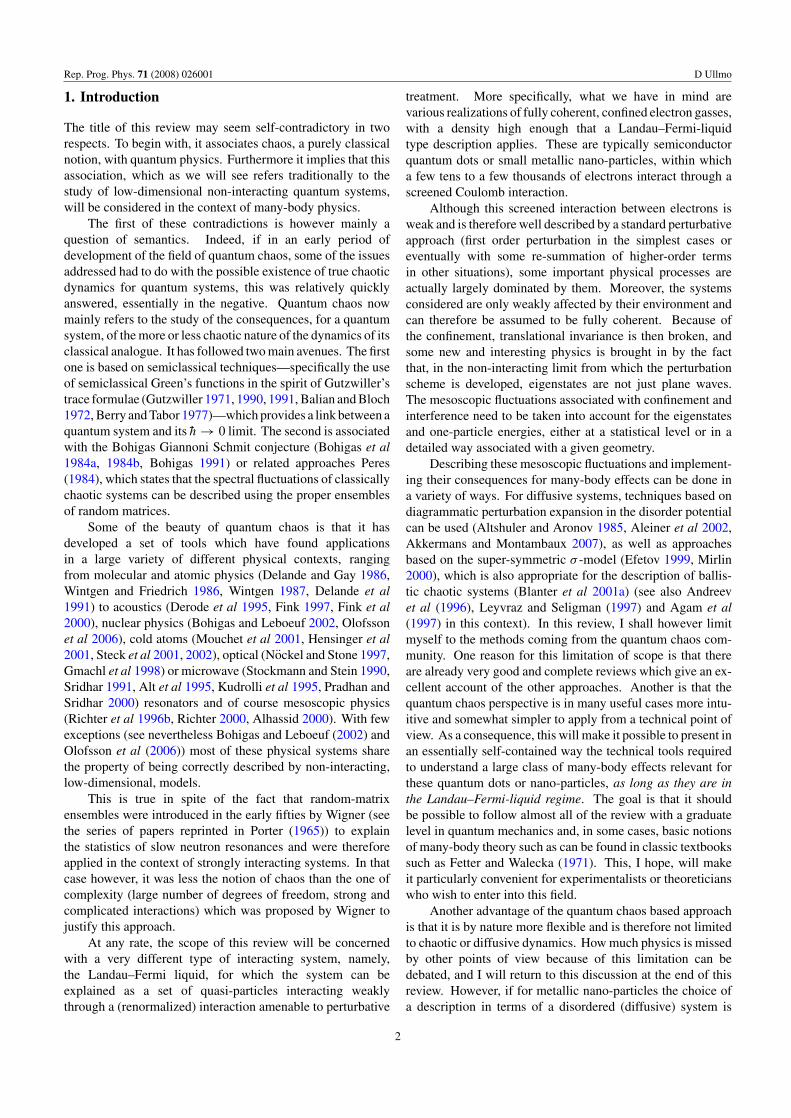
Figure 1. Direct terms of the Cooper series for the perturbativeexpansion of the thermodynamic potential �. Reprinted withpermission from Ullmo et al 1998. Copyright 1998 by the AmericanPhysical Society.
interaction lines (each of which yields a factor ν−10 ), k pairs
of Green’s functions and (k + 1) summations of Matsubarafrequencies (each of them associated with a factor β−1). Asfar as powers of h are concerned, |G|2 ∼ ν0/h (whateverthe dimension). Therefore, the only delicate point here is torealize that each temperature factor β−1 should be accountedfor as an h, since in the mesoscopic regime considered here,the time tT = hβ/π introduced above should be of the orderof some characteristic time tc of the system (say the time offlight), and thus β−1 ∼ h/tc ∝ h (again as far as powersof h are concerned). The kth term of the Cooper series istherefore of order [1/ν0]k[ν0/h]k[h]k+1 ∼ h and thus scales ash independently of k. The RPA series can be seen, in the sameway, to be of order h, but the corresponding terms turn out tohave negligible magnetic field dependence and can thereforebe omitted from the calculation of the magnetic response.Moreover one can convince oneself that all other diagramswould, at some given order k, have either a smaller number ofGreen’s functions or a larger number of frequency summationsand therefore are of higher order in h.
Noting that, because interaction (3.14) is local, the directand exchange Cooper diagrams differ only by their sign and bya spin degeneracy factor, the magnetic response can be derivedfrom the Cooper series contribution to the thermodynamicpotential8:
�C = g2s − gs
2β
×∞∑
k=1
λk0
k
∑ωm<εF
∫dr1 . . . drk�(r1, rk; ωm) . . . �(r2, r1; ωm)
= g2s − gs
2β
∑ωm<εF
Tr{ln[1 + λ0�(r, r′; ωm)]}, (3.15)
where ωm = 2πm/β are (bosonic) Matsubara frequencies,
�(r, r′; ωm) = 1
βgsν0
∑εn<εF
G(r, r′; εn)G(r, r′; ωm − εn)
(3.16)
is the (free) particle–particle propagator and the finite range ∼λF of the interaction introduces a cutoff on the summation overMatsubara frequencies at the corresponding energy scale εF.
The trace over the space coordinates is a short way ofexpressing the expansion in all orders in λ0�. The concept ofthe particle–particle propagator, as well as the Cooper seriescontribution, comes from the Cooper pairs in the theory of
8 Note that the diagrammatic rules for � differ slightly from the ones forcorrelation functions. There is in particular a factor 1/k associated with eachterm of order k, thus the log.
superconductivity. The main difference in our case is that nowthe interaction is repulsive (thus the plus sign in the trace)and that we have lost translational invariance (therefore wecannot trade the operators for ordinary functions by going tothe momentum representation).
3.2.1. Semiclassical evaluation of the particle–particlepropagator. To proceed further with our semiclassicalformalism, it is useful to write the finite temperature Green’sfunction between points r and r′ for a fermionic Matsubarafrequency (or rather energy) εn = (2n+1)π/β in terms of theretarded and advanced Green’s functions as
G(r, r′; εn)= �(εn)GR(r, r′; εF + iεn)
+ �(−εn)GA(r, r′; εF +iεn), (3.17)
with εF the Fermi energy. The retarded and advancedGreen’s functions are related through (3.7) and expressed, ina semiclassical approach, as expansions over all trajectoriesj joining r′ and r at energy ε (see (2.3)). The complexenergy-arguments of (3.17) force us to perform some analyticcontinuation. However, if the Matsubara energies are muchsmaller than εF, one can expand the classical action and use(2.7) to obtain
GRj (r, r′; εF +iεn) = GR
j (r, r′; εF) × exp
[−εntj
h
]. (3.18)
Note that, as in (3.8), temperature introduces the time scaletT = hβ/π which exponentially suppresses the contributionsof long paths through the term εntj /h = (2n + 1)tj /tT.Therefore, only small Matsubara frequencies need to beconsidered, and the assumption used for the perturbativetreatment of the energy is consistent.
To compute the magnetic susceptibility at B = 0, the fielddependent part of the semiclassical Green’s function can alsobe treated perturbatively, and using (3.12) one can write
GRj (r, r′; εF +iεn; B) = GR
j (r, r′; εF; B =0)
× exp
[−εntj
h
]× exp
[i2π
Baj
φ0
], (3.19)
where aj is the effective area enclosed by the orbit (circulationof the vector potential between r′ and r) and φ0 the fluxquantum. The weak-field semiclassical approximation to(3.17) is then given by
G(r, r′; εn, B)= θ(εn)∑
j :r’→r
Dj√−2iπh3
eiSj /h−iπζj /2
× exp
[−εntj
h
]× exp
[i2π
Baj
φ0
]
+ θ(−εn)∑
j ′:r→r’
Dj ′√−2iπh3
e−iSj ′ /h+iπζj ′ /2
× exp
[εntj ′
h
]× exp
[−i2π
Baj ′
φ0
], (3.20)
where trajectories j and j ′ travel from r′ to r in oppositedirections, at energy εF, and in the absence of a magnetic field.
Note the usefulness of (3.20) goes beyond the problem oforbital magnetism discussed here, as it provides a calculational
12
Rep. Prog. Phys. 71 (2008) 026001 D Ullmo
(a) (b)
(d)(c)
Figure 2. Pairs of orbits contributing to �C (see (3.15) for a(non-integrable) billiard. Top row: first order contributions. Bottomrow: third order contributions (there are therefore three pairs oforbits connected at interaction points in both (c) and (d)). Leftcolumn: generic case. Right column: pairing of time-reversedtrajectories (diagonal contribution), for which the dynamical phasescancel. (Courtesy of Harold Baranger.)
approach to any perturbative problem where the single-particleclassical dynamics is known.
The particle–particle propagator �(r, r′; ωm) can now beevaluated semiclassically from (3.20) and (3.16). In generalthis involves a sum over all pairs of classical trajectoriesjoining r′ to r. An illustration is shown in figure 2. Asin section 3.1, however, most of these pairs yield highlyoscillating contributions which average to zero when integratedover position, and one should only consider the non-oscillatingterms which maintain a field dependence. One way to do thisis, again, to pair time-reversed trajectories, which implies thatin the sum over the fermionic Matsubara frequencies in (3.16),only the εn such that εn(ωm − εn) < 0 should be kept. Thisdiagonal part �(D) of the particle–particle propagator can thenbe written as
�(D)(r, r′; ωm) � kBT
gsh
∑j : r→r′
|Dj |2me
exp
[i4π
Baj
φ0
]
×εn<εF∑
εn(ωm−εn)<0
exp
[− (|εn|+|ωm−εn|)tj
h
]. (3.21)
Summing over εn in the contribution of trajectory j , one getsεn<εF∑
εn(ωm−εn)<0
exp
[− (|εn|+|ωm−εn|)tj
h
]
= exp
[−ωmtj
h
]R(2tj /tT)
2tj /tT
(1 − exp
[− (εF−ωm)t
h
]),
(3.22)
where the function R and the temperature time tT wereintroduced in the discussion of (3.9). The last factor(1 − exp[−(εF − ωm)t/h]) originates from the upper boundεF of the Matsubara sum. If one assumes ωm � εF, this factorremoves from �(D)(r, r′) all the contributions of trajectories oflength smaller than �0 = λF/π , thus preventing the particle–particle propagator from diverging as r → r′. Replacing it by
a hard cutoff at �0 one obtains
�(D)(r, r′; ωm) � kBT
gsh
∑j : r → r’Lj > �0
|Dj |2me
R(2tj /tT)
2tj /tT
× exp
[i4π
Baj
φ0
]exp
[−ωmtj
h
]. (3.23)
The semiclassical form for �(D)(r, r′; ωm) shares with HD andFD (equations (3.13a) and (3.13b)) the property of being asemiclassical expansion which does not oscillate rapidly (onthe scale of λF) as a function of the coordinates, as would bethe case for the Green’s functions (3.20).
4. Orbital magnetism: diffusive and ballistic systems
4.1. Diffusive systems
The semiclassical approach described above does not rely onany assumption concerning the character of the underlyingclassical dynamics. It is therefore applicable to (integrableor chaotic) ballistic structures (Ullmo et al 1998, von Oppenet al 2000) as well as to diffusive systems (Montambaux1996, Ullmo et al 1997). Because diffusive motion is insome sense relatively simple, it is natural to consider firstthe orbital magnetism of interacting systems whose non-interacting classical dynamics is diffusive. More specifically,I will discuss the interaction contributions to the persistentcurrent of metal rings and to the susceptibility of singlyconnected two-dimensional diffusive systems. We shall seethat in this case, the semiclassical approach recovers, in a verytransparent and intuitive way, results previously obtained byquantum diagrammatic calculations (Aslamazov and Larkin1975, Altshuler et al 1983, Ambegaokar and Eckern 1990b,Eckern 1991, Oh et al 1991). Applied to diffusive dynamics,the semiclassical approach is indeed on the same level ofapproximation. Moreover, by making the connection with theclassical dynamics, it provides a physically intuitive picture ofthe interplay between disorder and interactions.
We assume here that the Fermi wavelength λF is theshortest length scale, in particular λF < � with � the elasticmean free path, and that the magnetic field is classically weak,i.e. the cyclotron radius at the Fermi energy is such thatRc � �.Then the paths entering into (3.23) can be approximated bythose of the system at zero field, but include the presence ofthe disorder potential.
For diffusive systems it proves convenient to relate �(D)
to the (classical) conditional probability P εcl(r, r′; t |A) to
propagate from r′ to r in a time t and enclosing an area A sincethis probability satisfies a simple diffusion equation. For thispurpose let us introduce an additional time and area integration1 = ∫
dtδ(t − tj )∫
dAδ(A−aj ) in (3.23) in order to make useof the sum rule (2.24), which, for a two-dimensional kineticplus potential Hamiltonian, and including the constraint on thearea, reads∑j :r′→r
|Dj(ε)|2me
δ(t − tj )δ(A − aj ) = 2πP εcl(r, r′, t |A).
(4.1)
13
Rep. Prog. Phys. 71 (2008) 026001 D Ullmo
One therefore obtains
�(D)(r, r′; ωm)
� 2π
gs
kBT
h
∫dA
∫t>�0/vF
dt P εcl(r, r′, t |A)
R(2t/tT)
2t/tT
× exp
[i4π
BA
φ0
]exp
[−ωmt
h
]. (4.2)
In the same way the nth order (diagonal) con-tribution to the thermodynamic potential in (3.15) canthen be expressed through the joint return probabilityP(r1, rn, . . . , r1; tn, . . . , t1|A) to visit the n points ri under theconditions that ti is the time elapsed during propagation fromri to ri+1 and that the total enclosed area is A. For diffusivemotion the probability is multiplicative, namely,∫
with ttot = ∑ti . Upon inserting the sum rule (4.1) and the
relation (4.3) into (3.23), the contribution from the diagonalterms �(D) to � (see (3.15)) yields
�(D) =∑
n
�(D)n
= 1
β
∫dr
∫dt coth
(t
tT
)K(t)A(r, t; B). (4.4)
The factor coth(t/tT) (with tT defined by (3.8)) arises from theω-sum in (3.15) which can be performed here explicitly. In(4.4) the functions K and A are defined as
K(t) ≡∑
n
Kn(t);
Kn(t)≡ (−λ0)n
n
{∫ n∏i=1
[dtiR(2ti/tT)
gsti
]δ(t − ttot)
}, (4.5)
A(r, t; B) ≡∫
dA cos
(4πBA
φ0
)P(r, r; t |A). (4.6)
K(t) accounts for temperature effects while A(r, t; B)
contains the field dependence and the classical returnprobability.
4.1.1. Renormalization scheme for diffusive systems. Thissemiclassical approach allows us further to obtain therenormalization of the coupling constant (Altshuler et al 1983,Altshuler and Aronov 1985, Eckern 1991, Ullmo et al 1997)for diffusive systems by resuming the higher-order diagrams ofthe Cooper series. To this end let us first introduce the Laplacetransform of K1(t),
f (p) = 4λ0
gs
nF∑n=0
1
ptT + 2(2n + 1), (4.7)
where
nF = βεF
2π= kFLT
4. (4.8)
The full kernel K(t) is given by the inverse Laplace transform
K(t) = 1
2π i
∫ +i∞
−i∞dp e+pt ln[1 + f (p)]. (4.9)
To evaluate the above integral, let us define
g(p) ≡ 1 + f (p) (4.10)
and furthermore denote the singularities of g(p) by
pn = −2(2n + 1)
tT(4.11)
with n = 0, . . . , nF. Let pn be the corresponding zeros (pn isassumed to lie between pn and pn+1). On the real axis, g isa real function which is negative within each interval [pn, pn](with the notation pnF = −∞) and positive elsewhere. As aconsequence, ln g(p) is analytic everywhere in the complexplane except for the branch cut [pn, pn]. The phase jumpacross the branch cuts is 2π , since the imaginary part ofg(p) is positive above and negative below the real axis.Deforming the contour of integration as sketched in figure 3,one therefore finds
K(t) = limε→0
∫ 0
−∞
dp
2iπ(ln[g(p − iε)] − ln[g(p + iε)])ept
(4.12)
=nF∑
n=0
∫ pn
pn
dpept (4.13)
= 1
t
nF∑n=0
[epnt − epnt ]. (4.14)
For n � nF one has δn ≡ tT(pn − pn) � 1 and thus to firstorder in δn:
1 +λ0
gs
nF∑n′ �=n
1
n′ − n− 4λ0
gs
1
δn
= 0 . (4.15)
The above condition gives
δn = 4
gs/λ0 + �(nF + 1) − �(2n + 1)(4.16)
with � the digamma function.In the high temperature regime tT � t , all the ns actually
contributing to the sum (4.14) are such that the denominatorin (4.16) is dominated by �(nF + 1) � ln(nF). One obtains inthis case
K(t) = 1
t
nF∑n=0
epnt [1 − e−δnt/tT ] (4.17)
� 1
tT
4
ln(kFLT/4)
nF∑n=0
epnt . (4.18)
In the low temperature regime tT/t � 1, the typical n
contributing to (4.14) is n0 ≡ tT/4t (that is still assumed tobe much smaller than nF). Because of the slow variation ofthe logarithm, one can in this case replace n by n0 in (4.16).
14
Rep. Prog. Phys. 71 (2008) 026001 D Ullmo
g(p)
P1
P2
P2P3P3 P1
p [1/t ]T
P3P3 P2
P2 P
1P1
–15 –10 –5 0
Re(p)
Im(p)
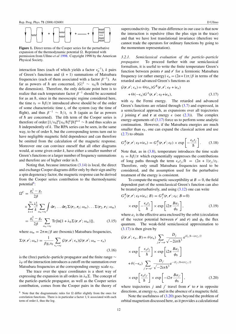
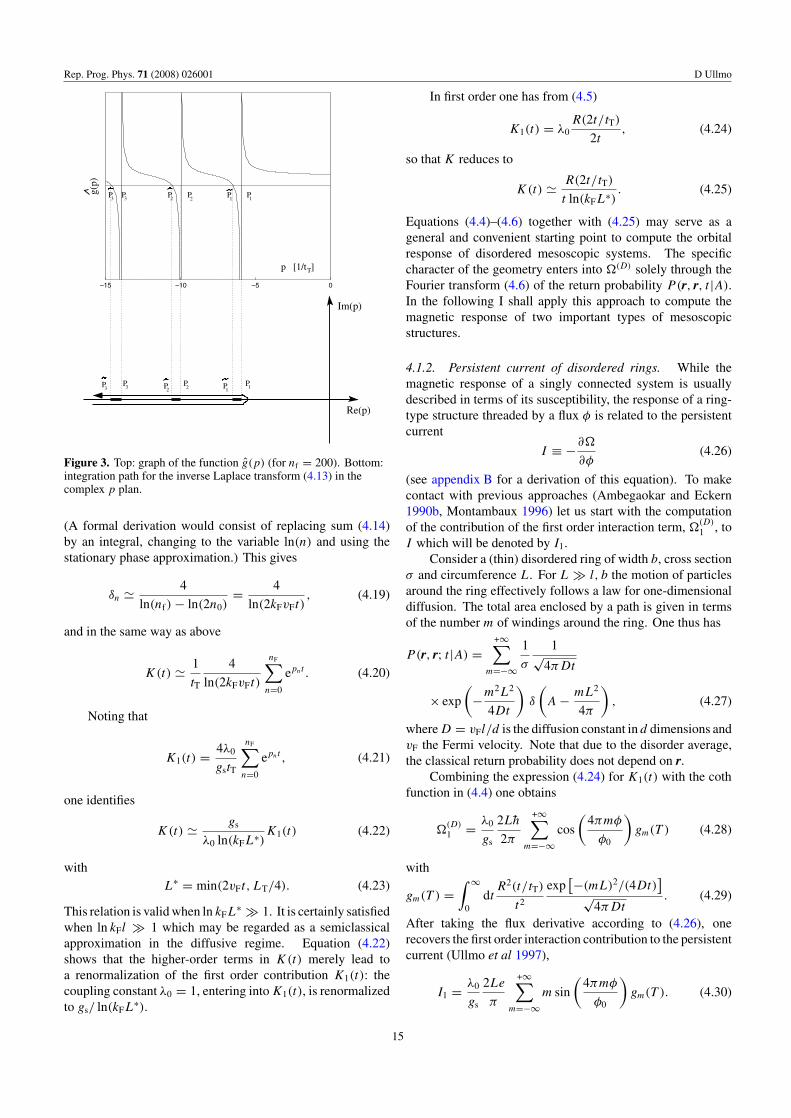
Figure 3. Top: graph of the function g(p) (for nf = 200). Bottom:integration path for the inverse Laplace transform (4.13) in thecomplex p plan.
(A formal derivation would consist of replacing sum (4.14)by an integral, changing to the variable ln(n) and using thestationary phase approximation.) This gives
δn � 4
ln(nf) − ln(2n0)= 4
ln(2kFvFt), (4.19)
and in the same way as above
K(t) � 1
tT
4
ln(2kFvFt)
nF∑n=0
epnt . (4.20)
Noting that
K1(t) = 4λ0
gstT
nF∑n=0
epnt , (4.21)
one identifies
K(t) � gs
λ0 ln(kFL∗)K1(t) (4.22)
withL∗ = min(2vFt, LT/4). (4.23)
This relation is valid when ln kFL∗ � 1. It is certainly satisfied
when ln kFl � 1 which may be regarded as a semiclassicalapproximation in the diffusive regime. Equation (4.22)shows that the higher-order terms in K(t) merely lead toa renormalization of the first order contribution K1(t): thecoupling constant λ0 = 1, entering into K1(t), is renormalizedto gs/ ln(kFL
∗).
In first order one has from (4.5)
K1(t) = λ0R(2t/tT)
2t, (4.24)
so that K reduces to
K(t) � R(2t/tT)
t ln(kFL∗). (4.25)
Equations (4.4)–(4.6) together with (4.25) may serve as ageneral and convenient starting point to compute the orbitalresponse of disordered mesoscopic systems. The specificcharacter of the geometry enters into �(D) solely through theFourier transform (4.6) of the return probability P(r, r, t |A).In the following I shall apply this approach to compute themagnetic response of two important types of mesoscopicstructures.
4.1.2. Persistent current of disordered rings. While themagnetic response of a singly connected system is usuallydescribed in terms of its susceptibility, the response of a ring-type structure threaded by a flux φ is related to the persistentcurrent
I ≡ −∂�
∂φ(4.26)
(see appendix B for a derivation of this equation). To makecontact with previous approaches (Ambegaokar and Eckern1990b, Montambaux 1996) let us start with the computationof the contribution of the first order interaction term, �
(D)1 , to
I which will be denoted by I1.Consider a (thin) disordered ring of width b, cross section
σ and circumference L. For L � l, b the motion of particlesaround the ring effectively follows a law for one-dimensionaldiffusion. The total area enclosed by a path is given in termsof the number m of windings around the ring. One thus has
P(r, r; t |A) =+∞∑
m=−∞
1
σ
1√4πDt
× exp
(−m2L2
4Dt
)δ
(A − mL2
4π
), (4.27)
where D = vFl/d is the diffusion constant in d dimensions andvF the Fermi velocity. Note that due to the disorder average,the classical return probability does not depend on r.
Combining the expression (4.24) for K1(t) with the cothfunction in (4.4) one obtains
�(D)1 = λ0
gs
2Lh
2π
+∞∑m=−∞
cos
(4πmφ
φ0
)gm(T ) (4.28)
with
gm(T ) =∫ ∞
0dt
R2(t/tT)
t2
exp[−(mL)2/(4Dt)
]√
4πDt. (4.29)
After taking the flux derivative according to (4.26), onerecovers the first order interaction contribution to the persistentcurrent (Ullmo et al 1997),
I1 = λ0
gs
2Le
π
+∞∑m=−∞
m sin
(4πmφ
φ0
)gm(T ). (4.30)
15
Rep. Prog. Phys. 71 (2008) 026001 D Ullmo
This first order result was first obtained by purelydiagrammatic techniques by Ambegaokar and Eckern (1990b)and semiclassically by Montambaux (1996).
However, higher-order terms are essential for anappropriate computation of the interaction contribution. Asshown in the preceding subsection, these higher-order termsmerely lead to a renormalization of the coupling constantaccording to (4.22). Thus the persistent current from the entireinteraction contribution is reduced to (Ullmo et al 1997)
I = 2Le
π ln(kFL∗)
+∞∑m=−∞
m sin
(4πmφ
φ0
)gm(T ). (4.31)
For diffusive rings the length scale vFt , entering in (4.23) forL∗, is given by Lm = vF(mL)2/4D, the average length of atrajectory diffusing m times around the ring. Hence one getsat a low temperature (LT � Lm) a (renormalized) prefactor∼2/ ln(kFLm) for I . At a high temperature, LT � Lm,the prefactor includes 2/ln(kFLT/4). These two limits agreewith the quantum results obtained diagrammatically by Eckern(1991). The functional form of the temperature dependence(exponential T -damping (Ambegaokar and Eckern 1990b)) isin line with experiments (Levy et al 1990, Chandrasekhar et al1991, Mohanty et al 1996). However, the amplitude of thefull persistent current with renormalized coupling constant isa factor ∼3–5 to small compared with experiments.
4.1.3. Susceptibility of two-dimensional diffusive systems. Inring geometries the exponential temperature dependence of I isrelated to the existence of a minimal length, the circumferenceof the ring, for the shortest flux-enclosing paths. In singlyconnected systems the geometry does not constrain returningpaths to have a minimal length, and therefore one expects adifferent temperature dependence of the magnetic response.
Consider a two-dimensional singly connected quantumdot with diffusive dynamics. If one makes use of the generalrenormalization property of diffusive systems, expressed by(4.25), the diagonal part of the thermodynamic potential (see(4.4)), including the entire Cooper series, reads
�(D) = 1
β
∫dr
∫ ∞
τel
dt1
ln(kFvFt)
tT
t2R2
(t
tT
)A(r, t; B).
(4.32)
The parameter L∗ appearing in (4.22) has been here replacedby vFt since the factor R2 ensures that the main contributionto the integral comes from t < tT. In the above time integralthe elastic scattering time τel = l/vF enters as a lower bound.This cutoff must be introduced since for backscattered pathswith times shorter than τel the diffusion approximation (4.33)no longer holds. Short paths with t < τel, which mayarise from higher-order interaction events, contribute to theclean bulk magnetic response (Aslamazov and Larkin 1975,von Oppen et al 2000). This latter term is, however, negligiblecompared with the disorder induced interaction contributionsconsidered here.
To evaluate the integral for A, the conditional returnprobability in two dimensions is conveniently represented in
terms of the Fourier transform (Argaman et al 1993)
P(r, r, t |A) = 1
8π2
∫dk|k| eikA
sinh(|k|Dt). (4.33)
Introducing the magnetic time
tB = φ0
4πBD= L2
B
4πD(4.34)
(tB is related to the square of the magnetic length L2B which can
be regarded as the area enclosing one flux quantum (assumingdiffusive dynamics)), one obtains
A(r, t; B) = 1
4πD
R(t/tB)
t. (4.35)
The function R occurring in (4.35) has a different origin thanin (4.32).
The magnetic susceptibility (3.3) is obtained afterincluding the expression (4.35) in (4.32) and taking the secondderivative with respect to the magnetic field. One finds, afternormalization to the Landau susceptibility of non-interactingparticles in a clean system,
χ(D)
|χL| = −12
π(kFl)
∫ ∞
τel
dt
t ln(kF vFt)R2
(t
tT
)R′′
(t
tB
).
(4.36)
Here, D = vFl/2, and R′′ denotes the second derivative of R.The above equation (4.36) holds true only as long as
the effective upper cutoff time t∗ ≡ min(tT, tB), introducedthrough the R-functions, remains smaller than the Thoulesstime tc = L2/D with L being the system size. For times largerthan tc the two-dimensional diffusion approximation is nolonger valid since the dynamics begins to behave ergodically.
Assuming τel � t∗ < tc, the integral in (4.36) can beapproximately evaluated by replacing the upper bound byt∗ and by replacing R(t/tT) and R′′(t/tB) by R(0) = 1and R′′(0) = −1/3, respectively. The averaged magneticsusceptibility of a diffusive two-dimensional quantum systemreads under these approximations (Ullmo et al 1997)
χ(D)
|χL| � 4
π(kFl) ln
{ln[kF vF min(tT, tB)]
ln(kFl)
}. (4.37)
The magnetic response of diffusive systems is paramagneticand enhanced by a factor kFl compared with the clean Landaususceptibility χL.
Contrary to the exponential temperature dependence ofthe ring geometry discussed in the previous section one finds alog–log temperature dependence for tT < tB as well as a log–log B dependence for tT > tB . The log–log form of the resultis produced by the 1/t ln t dependence of the integral in (4.36).It results from the wide distribution of path-lengths in thesystem—there are flux-enclosing paths with lengths rangingfrom about vFτel up to vFt
∗.Expression (4.37) agrees with results from Aslamazov and
Larkin (1975), Altshuler et al (1983) and Oh et al (1991) whichare obtained with quantum diagrammatic perturbation theory.The equivalence between the semiclassical and diagrammatic
16
Rep. Prog. Phys. 71 (2008) 026001 D Ullmo
approaches, demonstrated here as well as in the precedingsection for diffusive rings, may be traced back to the fact that‘quantum’ diagrammatic perturbation theory relies on the useof the small parameter 1/kF� and can therefore also be viewedas a semiclassical approximation.
4.2. Ballistic systems
We turn now to the magnetic response of ballistic mesoscopicobjects. This problem has attracted considerably less attentionthan the diffusive regime, partly because of the experimentaldifficulties involved, but also presumably because from thetheoretical point of view, ballistic systems cannot be addressedwith the more traditional approaches of solid state physics.Indeed, for diffusive systems, the main virtue of the ‘quantum-chaos’ based approach presented in this review was to providean alternative, maybe more intuitive, way to get known results.In contrast, the ballistic regime represents one example forwhich it is actually the only way to get an understanding of thephysics involved.
The ballistic character of the underlying classicaldynamics brings about some important differences, especiallysince one no longer talks about probabilistic concepts (likethe return probability), but one needs to input the informationabout specific trajectories. Depending on the geometry of theconfining potential, one can have chaotic or integrable motion,and the structure of the semiclassical expansions differs insome respects in these two cases. In particular, the existence offamilies of trajectories for integrable dynamics will translateinto a larger magnetic response.
4.2.1. Renormalization scheme for ballistic systems. As fordiffusive systems, (3.15) and (3.23) form the basic expressionsfrom which the magnetic response can be computed. We justsaw that in this latter case, they allow quite straightforwardlyto express the magnetic susceptibility of dots or persistentcurrent of rings in closed form. For ballistic systems onthe other hand, even when the classical dynamics is simpleenough to yield �(D)(r, r′; ωm) explicitly, taking the logarithmof this operator as implied by (3.15) will require proceedingnumerically. It should be borne in mind however that thisnumerical calculation is significantly simpler than the onewe would have faced had we decided to start directly witha numerical approach. This can be understood for instance byconsidering that the original operator �(r, r′; ωm), because ofits quantal nature, has a scale of variation determined by λF.Discretizing this operator on a grid would therefore requireusing a mesh containing at least a few points per λF, whichwould make any computation rapidly intractable as the sizeof the problem increases. On the other hand, within thesemiclassical approach, the operator one has to deal with is�(D)(r, r′) which, up to one exception to which I shall returnbelow, varies only on a classical scale. �(D)(r, r′) is thereforewhat one may call a ‘classical operator’. It permits the useof a grid mesh whose scale is fixed by the classical dynamicswithin the system and is therefore much larger than λF.
As mentioned above �(D)(r, r′) is not yet completelyclassical. Indeed, there is still, in (3.23), the scale �0 = λF/π
which specifies that trajectories shorter than �0 should beexcluded from the sum over trajectories joining r′ to r. This lastquantum scale can be removed using a simple renormalizationscheme where integration over short trajectories yields adecreased effective coupling constant. To this end considera new cutoff � larger than �0 but much smaller than anyother characteristic lengths (a, LT, or
√φ0/B). For each
path j joining r′ to r with Lj > �, let �j(r, r′) denotes itscontribution to �(D)(r, r′) and define
where the ri integration is over �0 < |ri−1 − ri | < �
(with r0 ≡ r′). �(r1, r′) is defined by (3.23) but with thesum restricted to ‘short’ trajectories with lengths in the range[�0, �]; �j(r, r1) is obtained from �j(r, r′) by continuouslydeforming trajectory j . To avoid the awkward ln in (3.15), letus introduce
� = 1
β
∑ωm
Tr
[1
1 + λ0�(D)(r, r′; ωm)
], (4.39)
from which �(D) can be derived through
�(D)(λ0) =∫ λ0
0
dλ′0
λ′0
�(λ′0). (4.40)
The replacement � by � in � amounts to a reordering ofthe perturbation expansion of � in which short paths aregathered into lower-order terms. Moreover, if Lj � �, smallvariations in the spatial arguments do not noticeably modifythe characteristics of �j . Approximating �j(r, r1) by �j(r, r′)in (4.38) and using �(r1, r′) � 1/4π |r1 − r′|2 valid for shortpaths, one obtains
λ0�j (r, r′) � λ0�j(r, r′)
1 + λ0∫
dr1�(r1, r′)� λ(�) �j (r, r′),
(4.41)
where the running coupling constant is defined by
λ(�) = λ0
1 + (λ0/gs) ln(�/�0). (4.42)
Therefore, these successive steps amount to a change in boththe coupling constant and the cutoff (since now trajectoriesshorter than � must be excluded) without changing �; that is,
�(�0, λ0) = � (�, λ(�)) . (4.43)
Through (4.40), this renormalization scheme can be applied to�(D) and so to the average susceptibility.
In this way, we have eliminated the last ‘quantum scale’�0 from the definition of �(D): � can be made much largerthan λF while remaining smaller than all classical lengths. Thiswill serve two purposes. From a quantitative point of view, itmeans that discretizing the operator �(D) can be done on arelatively coarse grid, and therefore operations such as taking
17
Rep. Prog. Phys. 71 (2008) 026001 D Ullmo
the trace logarithm of 1+�(D) that may be necessary to get themagnetic response can be done numerically much more easily.
Furthermore, it is qualitatively reasonable that theperturbation series of �(D) becomes convergent when � isof order of the typical size L of the system, since by thispoint the spread in length scales causing the divergence hasbeen eliminated. Of course the renormalization scheme givenabove assumes � to be much smaller than all the classicalscales of the system, and using � � L is beyond the rangefor which a reliable quantitative answer can be obtained. At aqualitative level however, this implies that higher-order termsin the diagonal contribution mainly renormalize the couplingconstant λ0 into
λ(L) = λ0
1 + (λ0/gs) ln(kFL). (4.44)
In the deep semiclassical limit ln(kFL) � 1, the originalcoupling constant λ0 drops from the final results and is replacedby gs/ ln(kFL).
For integrable systems in which non-diagonal channelsexist, a simple inspection shows that the latter are notrenormalized. Indeed the corresponding higher-order termsin the perturbation expansion are highly oscillatory. The non-diagonal contributions are therefore of order λ0 rather thangs/ ln(kFL) and will as a consequence dominate the magneticresponse in the deep semiclassical regime.
4.2.2. Ballistic squares. As an illustration, let us considersquare quantum dots. The choice of squares is motivated firstbecause this is the geometry used experimentally (Levy et al1993) and secondly because squares are particularly amenableto a semiclassical treatment, since it is very easy to enumerateall the classical trajectories9. To be more specific, I willconsider a square billiard model, of size L, with free motion(i.e. just a kinetic energy term) inside the the billiard andDirichlet boundary conditions on its border. An illustrationof the shortest (with non-zero area) closed orbit and of theshortest periodic orbit, for the classical version of the billiard,is given in figure 4.
Let us first discuss the diagonal contribution �(D) (3.15)to the thermodynamic potential. Because of the simplicity ofthe geometry, the explicit expression of �j(r, r′; ω) for anyorbit j joining r′ to r can be obtained quite straightforwardly(though the resulting expressions might be a bit cumbersomeand will thus not be given). At a given temperature T , theoperator �(D)(r, r′; ω) is then constructed by summing all suchcontributions for orbits of lengths shorter than the thermallength LT (see (3.8)). A numerical computation of �(D)
(and therefore, after derivation with respect to the magneticfield, of the magnetic susceptibility) can then be obtained byrepresenting �(D)(r, r′; ω) on a grid, then going to a diagonalrepresentation, and in this diagonal representation taking thelog and performing the trace. The temperature dependence of
9 As a consequence of the two previous facts, orbital magnetism in ballisticsquares has been thoroughly studied within non-interacting models (Gefenet al 1994, VonOppen 1994, Ullmo et al 1995, Richter et al 1996a, 1996b,1996c).
Figure 4. Typical pairs of real-space trajectories that contribute tothe average susceptibility to first order in the interaction in thediagonal channel (left) and the non-diagonal channel (right).Reprinted with permission from Ullmo et al (1998). Copyright 1998by the American Physical Society.
Figure 5. Temperature dependence of the zero-field susceptibility(solid line) for an ensemble of squares at kFL = 50. Thecontribution of the non-diagonal channel (dashed, family (11) andrepetitions) exceeds that of the diagonal Cooper channel (dotted) atlow temperatures. Temperatures are expressed in units ofkBT0 = hvF/2πL. Inset: same, but with a different scale for thevertical axis. Reprinted with permission from Ullmo et al (1998).Copyright 1998 by the American Physical Society.
the resulting contribution to the susceptibility, for a number ofparticles corresponding to kFL = 50, is shown as a dotted linein figure 5.
In this way, one can further check that the renormalizationprocess described above actually works for the squaregeometry. For instance, figure 6 shows the value of themagnetic susceptibility at zero field, and for a temperaturesuch that LT = 4L, as a function of the cutoff �. As longas � � L, the diagonal part of the susceptibility is clearlyindependent of the cutoff if the renormalized interaction λ(�)
given by (4.42) is used.Let us finally compare the diagonal and non-diagonal
contributions. This latter is built from pairs of orbits withthe same action (i.e. for a billiard, same length) but differentgeometry, overlapping at a given point. These may occurquite generically for integrable systems for which familiesof periodic orbits exist and two members of the same familymay intersect in the configuration space. An illustration ofsuch an intersection is given in the right panel of figure 4 forthe family (labelled (1, 1)) of shortest periodic orbits (withnon-zero enclosed area) of this system. In the square billiard,
18
Rep. Prog. Phys. 71 (2008) 026001 D Ullmo
Log(Λ0/L) Log(10–1
) –3.0 –2.0
Log(Λ/L)
0.0
0.5
1.0
1.5
2.0
2.5
3.0
χ/χ L
(B=0, kFL=50, LT =4L)
λ=λ0
λ=λ(Λ)
Figure 6. Diagonal part of the interacting contribution to themagnetic susceptibility as a function of the cutoff � used to definethe particle–particle propagator �. The data correspond to zeromagnetic field, kFL = 50, and a temperature T such that LT = 4L.Solid line: computation for which the coupling constant λ varies as afunction of � following (4.42). Dashed line: λ is kept fixed (= λ0).The vertical (dashed) line corresponds to the limit of the range forwhich the condition � � L is fulfilled.
for a given closed orbit j of length Lj and enclosing an areaaj , the action in the absence of magnetic field is given byS0
j /h = kFLj , its derivative with respect to the magnetic fieldby dSj/dB = 2πaj /φ0 and the stability determinant (cf (2.5))by Dj = m/
√hkFLj . The contribution χ(1,1) of the pairs of
orbits from the family (1, 1) can for instance be derived quitestraightforwardly from equations (3.11a) and (3.11b) notingthat L11 = 2
√2L and a11 = 2x0(L − x0) (x0 is the abscissa
of the intersection of the orbit with the bottom border of thebilliard and can be used to label an individual orbit within thefamily (1, 1)). One obtains in this way (Ullmo et al 1998)
〈χnon-diag(1,1) 〉|χL| = − 3kFL
2(√
2π)3
d2C2(ϕ)
dϕ2R2
(L11
LT
). (4.45)
The temperature dependence is governed by the functionR(x) = x/ sinh(x) and the field dependence byC(ϕ) = (2ϕ)−1/2[cos(πϕ)C(
√πϕ) + sin(πϕ)S(
√πϕ)], with
ϕ = BL2/φ0 and C and S being Fresnel functions.As seen in figure 5, because the non-diagonal contribution
is not renormalized by higher-order terms, it dominates themagnetic response as soon as the temperature is low enoughnot to suppress it.
4.3. Discussion
After this overview of some of the results that can be derivedfor the magnetic response of mesoscopic rings or dots withina Fermi-liquid, at equilibrium, description, it is worthwhile tocome back to how well existing experiments can be understoodwithin this framework. Since the typical response for a singlesystem (Mailly et al 1993, Chandrasekhar et al 1991) may insome cases be dominated by the non-interacting contribution,
which is not addressed here, I will however limit this discussionto experiments done on ensembles of micro-structures.
Ballistic and diffusive systems differ with respect tothe comparison between experimental measurements andtheoretical predictions, but for both cases there is clearly notcomplete adequacy.
In the case of ballistic systems (Levy et al 1993), theamplitude of the magnetic response in the low temperaturerange, as well as the scale of the field dependence, is well inline with the predictions (von Oppen 1994, Ullmo et al 1995,Richter et al 1996b). However, the temperature dependence,and in particular the fact that a magnetic response is observedeven when the thermal length LT is smaller than the size of thesystem, seems very difficult to interpret within the Fermi-liquidframework used here (Ullmo et al 1995, 1998). There is, up tonow, no real suggestion to explain how a significant magneticresponse, with a field scale unambiguously associated withinterference effects, could survive at such high temperatures.
For diffusive rings (Levy et al 1990), the temperaturedependence seems to be less of an issue than in the ballisticcase. However the magnitude of the average persistentcurrent appears to be quite a bit larger (a factor 3 to 5)than what is expected theoretically (Ambegaokar and Eckern1990a). It has been suggested that this large magneticresponse might be related to non-equilibrium effects, suchas the coupling to a phonon or photon bath (Mohanty 1999,Kravtsov and Altshuler 2000, Entin-Wohlman et al 2003). Inlater experiments (Jariwala et al 2001) (see also Reulet et al(1995) and Deblock et al (2002) in this context), a further,and presumably more dramatic, discrepancy is that the signof the magnetic response—which has not been determined inLevy et al (1990)—was furthermore not the one expected fora repulsive interaction. This has motivated consideration ofwhether a BCS interaction, weak enough to be compatiblewith the absence of an observed superconducting state for theconsidered materials, could be responsible for both the changein sign (which would be an immediate consequence of havingan attractive interaction) and the increase in the magnitude ofthe observed signal (Schechter et al 2003, 2004, Eckern et al2004). It is not clear however that such a range of attractiveinteractions actually exist in practice.
In the end, it is remarkable that on the one hand a goodpart of the experimental findings has a simple and naturalinterpretation within the ‘confined electron gas with weakinteraction’ picture developed here, while on the other handno consensus has emerged as yet concerning the interpretationof other significant experimental findings. One of the limitingfactors in this respect is presumably the imbalance betweenthe large number of theoretical works and the much sparsercharacter of experimental studies on these questions. Inparticular, only one group has measured the magnetic responseof an ensemble of micro-structures in the ballistic regime(Levy et al 1993). In this case the low temperature data agreevery well with the theoretical description when there is littlehope to interpret what is observed in the high temperatureregime without introducing some new physical mechanisms.However, the lack of experimental indications of what theseother mechanisms could be is making any theoretical progress
19
Rep. Prog. Phys. 71 (2008) 026001 D Ullmo
difficult. In the same way, for diffusive systems, a completeunderstanding would be made easier if one knew how muchthe sign of the magnetization observed in Jariwala et al (2001)is material dependent.
Obviously, it would be very non-trivial to improve onthe existing experiments, in particular because it is necessaryto deal properly with very weak magnetic fields. However,there are enough indications that some deep physics might beinvolved to motivate further experimental work in this field.
5. Mesoscopic Kondo effect
Turning now to another context where the interrelation betweeninterferences and interactions plays an important role, I shallwander briefly away from Fermi liquids and consider some(limited) aspects of the problem of a Kondo impurity within amesoscopic conductor.
5.1. A quick background
The term ‘Kondo effect’ refers to the physics of an impuritywith some internal degree of freedom, interacting with a gasof otherwise non-interacting electrons. It represents one ofthe simplest models in condensed matter physics for whichcorrelations play a central role (Hewson 1993).
In its simplest version, the s–d model, the impurity is justtreated as a spin one half interacting locally with the electrongas. The corresponding Hamiltonian then reads
HK =∑ασ
εαc†ασ cασ + Hint, (5.1)
where c†ασ creates a particle with energy εα , spin σ and
wave-function ϕα(r), and the interaction with the impurity isexpressed as
Hint = J0
h2 S · s(0), (5.2)
with J0 the coupling strength, S = (Sx, Sy, Sz) aspin operator (h−1Si is half of the Pauli matrix σi),s(0) = h
2 �†σ (0)σσσ ′�σ (0) the spin density of the electron gas
at the impurity position r ≡ 0 and �†σ (0) = ∑
α ϕα(0)c†α .
Originally, physical realizations of the Kondo Hamilto-nian corresponded to actual impurities (e.g. Fe) in a bulk metal(e.g. Cu). The wave-functions ϕα could then be taken as planewaves, and one could assume a constant spacing � between theεα , so that the electron gas could be characterized by only twoquantities: the local density of states ν0 = (A�)−1 (A is thevolume of the sample) and the bandwidth D0 of the spectrum.
What gave (and still gives) to the Kondo problem itsparticular place in condensed matter physics is that it isthe simplest problem for which the physics is dominated byrenormalization effects. Indeed, assuming the dimensionlessconstant J0ν0 � 1, it can be shown using the one-loop renormalization-group analysis (Fowler and Zawadowzki1971) or equivalent earlier approaches such as Anderson’spoor man’s scaling (Anderson 1970) or Abrikosov’s parquetdiagrams re-summation (Abrikosov 1965) that the low energyphysics remains unchanged by the simultaneous modification
of both J0 and D0 into new values Jeff and Deff provided theyare related by
Jeff(Deff) = J0
1 − J0ν0 ln(D0/Deff). (5.3)
The renormalization procedure should naturally be stoppedwhen Deff becomes of the order of the temperature T of thesystem. Equation (5.3) defines an energy scale, the Kondotemperature
TK = D0 exp(−1/(J0ν0)), (5.4)
which specifies the crossover between the weakly and stronglyinteracting regime. For T � TK, the impurity is effectivelyweakly coupled to the electron gas, and the properties ofthe system can be computed within a perturbative approachprovided the renormalized interaction Jeff(T ) is used. Theregime T � TK is characterized by an effectively verystrong interaction (in spite of the bare coupling valueJ0ν0 being small), in such a way that the spin of theimpurity is almost completely screened by the electron gas.Perturbative renormalization analysis (and thus (5.3) itself)can obviously not be applied in this regime, but (for a bulksystem) a rather complete description has been obtained bya variety of approaches, including numerical renormalizationgroup (Wilson 1975), Bethe anzatz techniques (Andrei 1980,Wiegmann 1980) and in the very low temperature regimeNozières’ Fermi-liquid description (Nozieres 1974).
One important consequence of the scaling law (5.3) is thatphysical quantities can be described by universal functions,which can be understood by a simple counting of the number ofparameters defining the s–d model in the bulk. I will illustratethis discussion with a particular physical quantity, namely, thelocal susceptibility
χloc =∫ β
0dτ 〈Sz(τ )Sz(0)〉, (5.5)
which is the variation of the impurity spin magnetization toa field applied only to the impurity. The electron gas ischaracterized by its local density of states ν0 and its bandwidthD0, and the impurity by the coupling constant J0. Therefore,for a given temperature T , χloc, as any physical quantity, candepend only on these four parameters. Furthermore, only twodimensionless parameters can be constructed from them, theratio T/D0 and the product J0ν0. However, because of thescaling law (5.3), we see that these two parameters turn outto be eventually redundant. A dimensionless quantity cantherefore be expressed as a function of a single parameter,which can be chosen to be T/TK so that we have for instance
T χloc = fχ(T /TK), (5.6)
with fχ(x) a universal function which has been computedby Wilson (1975) using his numerical renormalization-groupapproach. Note finally that within the one-loop approximation(5.3) and (5.4),
T/TK = exp(Jeff(T )ν0), (5.7)
so that another way to express the universal character ofphysical quantities is to say that they depend only on thedimensionless quantity Jeff(T )ν0.
20
Rep. Prog. Phys. 71 (2008) 026001 D Ullmo
5.2. Mesoscopic fluctuations
We see that the universal character of the Kondo physics is adirect consequence of the fact that the local density of states isflat and featureless and can therefore be characterized by twoparameters, ν0 and D0. There are many situations howeverfor which the variation in energy (and position actually) of thelocal density of states νloc(r; ε) might be significantly morecomplex, and it is natural to ask in which way this wouldmodify the description given above in the bulk (flat band) case.
The origin of fluctuations in the density of states can beof different nature, but they are always in the end associatedwith interference or finite size effects. One possibility isthe presence of disorder in a bulk material (Dobrosavljevicet al 1992, Kettemann 2004, Kettemann and Mucciolo 2006,2007, Zhuravlev et al 2007), in either the metallic or thelocalized regime. Another is the proximity of some boundaryin the host material (Ujsaghy et al 2001), for instance, in thecase of a narrow point contact (Zarand and Udvardi 1996)or for thin films (Crepieux and Lacroix 2000). Finally theclass of systems where a Kondo impurity is placed within afully coherent, finite size electron sea, as has been realizedfor instance in the context of ‘quantum corrals’ (Fiete et al2001), has been also considered (Thimm et al 1999, Affleckand Simon 2001, Cornaglia and Balseiro 2002a, 2002b, 2003,Simon and Affleck 2002, Franzese et al 2003, Kaul et al 2005,2006, Lewenkopf and Weidenmuller 2005, Simon et al 2006).
One important recent development which has made verynatural the idea that a magnetic impurity could be connected toa finite size electron gas is the realization that Kondo physicswas actually relevant to transport properties of quantum dots(Glazman and Pustilnik 2005). Indeed, as was pointed outby Glazman and Raikh (1988) and simultaneously by Ng andLee (1988), a quantum dot in the deep Coulomb-blockaderegime (so that particle number fluctuations are suppressed)containing an odd number of electrons, and sufficiently smallsuch that the temperature can be made much smaller thanthe mean level spacing between orbitals, can be describedby an Anderson impurity model, which, up to a Schrieffer–Wolff transformation, is essentially equivalent to a Kondoimpurity. When the dot is weakly coupled to leads, the latterplay the role of the electron gas. In the low temperature regimeT � Tk, a correlated state is formed which mixes the quantumdots and both drain and source wave-functions, leading to alarge conductance (�e2/h) in spite of the dot being in thedeep Coulomb-blockade regime. These predictions have beenobserved by Goldhaber-Gordon et al (1998) a decade after theywere formulated, some later experimental realizations evenreaching the unitarity limit (van der Wiel et al 2000).
The great flexibility in the design and control ofnanoscopic systems further motivated the study of manynew configurations involving more exotic Kondo ef-fects. One can cite for instance the theoretical design(Oreg and Goldhaber-Gordon 2003) and experimental obser-vation (Potok et al 2007) of the 2-channel Kondo, which hasproved to be elusive in bulk systems, the possible occurrenceof SU (4) Kondo (Borda et al 2003, Le Hur and Simon 2003,
Le Hur et al 2004, Galpin et al 2005, Hur et al 2007) and itsrelevance to carbon nanotubes (Choi et al 2005, Makarovskiet al 2007a, 2007b) or the double dot system where Kondophysics might be in competition with RKKY interactions(Craig et al 2004, Simon et al 2005, Vavilov and Glazman2005, Martins et al 2006).
The subject of Kondo physics and quantum dots is a veryvast, and still rapidly developing, field. It is clearly not realisticto cover it in any reasonable way here, and I will only considerin more detail the, admittedly rather specific, aspects moreclosely related to the subject of this review. Indeed most of themore exotic designs imply at some point that a small quantumdot playing the role of a quantum impurity is connected to alarger mesoscopic object, for which Kondo physics in itselfis irrelevant, but such that finite size effects may becomeimportant. In other words, the context of Kondo physicsand quantum dots makes it almost unavoidable to considersituations where the ‘quantum impurity’ is connected to anelectron gas for which finite size effects are important.
As a consequence, for each such mesoscopic electronreservoir connected to the quantum impurity, two new energyscales enter into the description of the Kondo problem: thecorresponding mean level spacing �R and Thouless energyETh. The existence of a finite mean level spacing of theelectron reservoir will, for instance, clearly modify the Kondophysics drastically for low temperature T � �R . This willaffect the conductance (Thimm et al 1999, Simon and Affleck2002, Cornaglia and Balseiro 2003) as well as thermodynamicproperties (Cornaglia and Balseiro 2002a, Franzese et al 2003,Kaul et al 2005), and considerable insight can be gained byconsidering the properties of the ground states and first fewexcited states of the system (Kaul et al 2006, 2008).
The range of energy between �R and ETh is furthercharacterized by the presence of mesoscopic fluctuations (at allscales in this range) in the local density of states of thereservoir’s electron and thus by the fact that the density ofstates is not flat and featureless. In particular, one may wonderwhether a (eventually fluctuating) Kondo temperature can bedefined and if physical quantities remain a universal functionof the ratio T/TK.
To fix the ideas, let us consider the s–d Hamiltonian (5.1)
with a local density of states at the impurity site ν(r = 0; ε)def=∑
i |ϕi(0)|2δ(ε − εi). In the semiclassical regime, ν(r = 0; ε)
can be written as the sum
ν(ε) = ν0 + νfl(ε), (5.8)
where ν0 is the bulk-like contribution (2.12) (one should ofcourse include here either a realistic band dispersion relationor a cutoff at D0 to account for the finite bandwidth), and thefluctuating term νfl(ε) is a quantum correction associated withthe interfering closed orbit contributions (2.15). Because νfl(ε)
is the sum of rapidly oscillating terms, it will fluctuate not onlywith respect to the energy ε, but also with respect to the positionr of the quantum impurity or with respect to the variation of anyexternal parameter that may affect the classical actions Sj (2.4)on the scale h. As a consequence, one may think of νfl(ε) asa statistical quantity with different realizations corresponding
21
Rep. Prog. Phys. 71 (2008) 026001 D Ullmo
to various locations of r or obtained by varying an externalparameter in such a way that the classical dynamics remainsunmodified, but that the phases exp(iSj/h) are randomized.
Let us denote T 0K the Kondo temperature of the associated
bulk system for which ν(ε) is replaced by ν0. For T � T 0K it is
possible to use a perturbative renormalization-group approachin the same way as in the bulk, but including the mesoscopicfluctuations of the density of states. Following Zarand andUdvardi (1996), this gives in the one-loop approximation
Jeff(Deff) = J0
1 − J0∫ D0
Deff(dω/ω) νβ(ω)
, (5.9)
with
νβ(ω) = ω
π
∫ ∞
−∞dε
νloc(ε)
ω2 + ε2(5.10)
the temperature smoothed density of states (note that therenormalization up to order two loops was given by Zarandand Udvardi (1996)).
There are two different ways to use the aboverenormalization-group equation. For some physicalrealizations, the fluctuations of the local density of states maybe very significant, yielding an even larger variation of theKondo properties because of the exponential dependence in(5.4). In this case, one is mainly interested in the fluctuations ofthe Kondo temperature (which is now a functional of the localdensity of states) defined as the energy scale separating theweak and strong coupling regimes. One can then use the sameapproach as in the bulk and define TK[νβ] as the temperatureat which the one-loop effective interaction diverges, giving theimplicit equation
J0
∫ D0
T ∗K [νβ ]
dω
ωνβ(ω) = 1. (5.11)
Examples of systems for which the fluctuations of the densityare large enough to justify that one is mainly interested inthe fluctuation of the scale T ∗
K defined by (5.11) include,for instance, the case of ‘real’ (chemical) impurities in ageometry such that one dimension is not much larger thanthe Fermi wavelength. This may be either a quantumpoint contact in a two-dimensional electron gas (Zarand andUdvardi 1996) or a thin three-dimensional film (Crepieuxand Lacroix 2000). In this case there is a high probabilitythat the impurity is located at a place at which the Friedeloscillations (i.e. the term in the oscillating part of the densityof states associated with the trajectory bouncing back on theboundary and returning directly to its starting point) are large.In this case, the impurities located at a distance from theboundary such that the interference of the returning orbit isconstructive have a significantly larger Kondo temperature.Disordered metals near or beyond the localization transitionprovide another kind of system with large fluctuations ofthe local density of states and can lead in this particularcase to a finite density of ‘free moments’ for which theT ∗
K[νβ] corresponding to the space location is actually zero(Kettemann and Mucciolo 2007, Zhuravlev et al 2007).
In a typical ballistic or disordered-metallic mesoscopicsystem with all dimensions much larger than the Fermi
wavelength, the fluctuating part of the local density of states νfl
is a quantum correction to the secular term ν0 and is thereforeparametrically smaller. As a consequence the fluctuations ofTK[νβ(ω)] defined by (5.11) are not very large compared withT 0
K, which if it is taken only as an energy scale is somewhatmeaningless.
In the bulk case, TK has however, beyond being anenergy scale, another meaning which is to be the parameterentering into universal functions such as fχ in (5.6). Withinthis framework, TK is directly (and quantitatively) related tophysical observables, and its fluctuations need not be large tobe relevant.
In the mesoscopic case, however, there is a priori noreason for any physical observable to be a universal function,since the number of ‘parameters’ defining the problem can beconsidered as infinite (in the sense that one needs an infinitenumber of parameters to define the function ν(ε)). For agiven temperature T > T 0
K however, it is possible to performthe perturbative renormalization-group analysis leading to theeffective interaction strength Jeff(T ), (5.9), which amountsto integrating out all degrees of freedom corresponding toenergies larger than T . One can assume moreover that thefeatures of the density of states at energies smaller than T willnot affect the observables at temperature T . As a consequence,after renormalization, physical quantities can depend onlyon the parameters T , Jeff(T ) and νβ(T ). Dimensionalanalysis then implies that dimensionless quantities such asT χloc(T ) can depend only on one single parameter, the productJ (T ) = νβ(T )Jeff(T ). In particular T χloc(T ) should be equalfor an arbitrary mesoscopic realization and for some bulksystem with, at temperature T , the same value of the parameterJ (T ). This implies that if one defines the realizationand temperature dependent Kondo temperature TK[νβ](T )
by the generalization of (5.7) to the mesoscopic case,namely,
TK[νβ](T ) = T
exp(Jeff(T )νβ(T )), (5.12)
one obtains, within the one-loop approximation, a quantitativeprediction for physical quantities in the mesoscopic case. Forinstance, one has for the local susceptibility
which relates the universal function fχ , computed for the bulk,to the impurity susceptibility in the mesoscopic case.
From a practical point of view, however, one may firstnote that with definition (5.12), TK[νβ](T 0
K) = T ∗K[νβ] is
the same as the one obtained from (5.11). Furthermore,one finds that there is in general little difference betweenfχ(T /TK[νβ](T )) and fχ(T /T ∗
K[νβ]) in a large range oftemperatures above T 0
K. Therefore, although only (5.13)can be formally justified, I will continue the discussionassuming that in the high temperature regime T � T 0
K, thesusceptibility can be described by the universal formfχ(T /T ∗
K)
with a realization (but not temperature) dependent T ∗K defined
by (5.11).It turns out that this approach gives a very precise
prediction, provided T 0K is computed from a fit or the two-loop
22
Rep. Prog. Phys. 71 (2008) 026001 D Ullmo
approximation, and one uses T ∗K = T 0
K + δTK with δTK
defined by
J0
∫ D0
T 0K +δTK
dω
ω(ν0 + δνβ(ω)) = J0
∫ D0
T 0K
dω
ων0. (5.14)
Kaul et al (2005) and Yoo et al (2005) showed, by comparisonwith the exact numerical quantum Monte-Carlo calculations,that, even if one neglects the temperature variation of TK[νβ],the predictions from (5.13) are quantitatively extremelyprecise, even up to temperatures somewhat below T 0
K. Thisapproach therefore provides a simple and quantitative way todiscuss the mesoscopic fluctuations of the Kondo properties inthe temperature regime T � T 0
K.The nice thing here is that in this form, all the fluctuations
of physical quantities in this regime are expressed in terms ofthe local density of states that we know how to relate to classicalclosed orbits. Indeed, (5.14) can be rewritten for δTK � T 0
K as
δTK
T 0K
= ν−10
∫T 0
K
dω
ωνβ(ω). (5.15)
Furthermore using that νβ(ω) = νloc(εF +iω) and the analyticalcontinuation of (2.3) for complex energies in the same way as in(3.18), one can immediately relate the realization dependentKondo temperature T ∗
K[νβ] to a sum over orbits starting andending at the impurity site r0 = 0
δTK
T 0K
� 1√2π3h3 ν0
∑j :r0→r0
Dj sin
[1
hSj (ε) − ζj
π
2+
π
4
]
×∫ ∞
T 0K
dω
ωexp(−tjω/h). (5.16)
The last integral can be approximated by log(T 0
K tjh
)×exp(−tj T
0K/h), thus providing a cutoff for trajectories with
a time of return tj larger than h/T 0K. From this result, the
variance of the Kondo temperature can then be obtained.Pairing a trajectory only with itself and, if the electron gas istime-reversal invariant, with its time-reversal symmetric, andusing the sum rule (2.24), one has
〈δTK2〉
T 0K
2 � βRMT
πhν0
∫ Dcut
T 0K
dω′1
ω′1
dω′2
ω′2
∫ ∞
0dtP ε
cl(t)e−(ω′
1+ω′2)t/h,
(5.17)
with P εcl(t) the classical probability of return and βRMT = 1 for
a time-reversal non-invariant and 2 for a time-reversal invariantelectron gas.
For chaotic systems, using the model (2.26) and (2.27) forthe classical probability of return then immediately gives
〈δTK2〉
T 0K
2 � (2βRMT ln 2)
π
�
T 0K
. (5.18)
Interestingly, the same result can be derived from a random-matrix description (Kettemann 2004, Kaul et al 2005).Indeed, using (5.15), the variance of δTK can be expressed
in terms of the correlator
R2(ω1, ω2)def= 1
ν20
∫ω1
∫ω2
dω′1dω′
2〈νβ(ω′
1)νβ(ω′2)〉
ω′1ω
′2
(5.19)
= 1
π2ν20
∫ω1
∫ω2
dω′1dω′
2
×∑α1α2
〈(|ϕα1 |2 − 1/A)(|ϕα2 |2 − 1/A)〉[(µ − εα1)
2 + ω′1
2][(µ − εα2)2 + ω′
22]
.
(5.20)
Within the random-matrix model, the wave-functions have aPorter–Thomas distribution ((2.33) or (2.34)), and, neglectingthe correlations between eigenstates, which introduce only1/g corrections, one has 〈(|ϕα1 |2 − 1/A)(|ϕα2 |2 − 1/A)〉 =δα1α2(βRMT/A2). Neglecting the fluctuations of the eigenergiesεα and performing the integral, one then gets
R2(ω1, ω2) = βRMT�
π
(1
ω2ln
ω1 + ω2
ω1+
1
ω1ln
ω1 + ω2
ω2
),
and thus R2(T0
K, T 0K) = 2 ln 2(βRMT�/πT 0
K), from which(5.18) derives immediately (Kaul et al 2005). Within therandom-matrix description, the full distribution of TK has beenobtained by Kettemann (2004).
To conclude this section, we see that the mesoscopicfluctuations of Kondo properties provide an example ofphysical systems where relatively non-trivial information iseventually encoded in the classical trajectories. Moreoverthrough the sum rule (2.24) and the model (2.26) and (2.27)for the classical probability of return P ε
cl(t), a connection withrandom-matrix theory can be made.
It should be stressed however that the most interestingaspect of this mesoscopic Kondo problem, namely,the fluctuations of physical properties in the deep Kondoregime (� <) T � T 0
K, is still an open problem. Thisregime should be characterized by much larger fluctuations,which should be therefore easier to observe experimentally,as well, as has already been seen in exact numerical Monte-Carlo calculations (Kaul et al 2005), as a lack of universality.The perturbative renormalization-group point of view used inthe high temperature regime will clearly not be applicableat those temperatures, but Fermi-liquid descriptions based onmean-field slave-boson techniques should nevertheless be ableto shed some light on the physics dominating the mesoscopicfluctuations in this regime (Burdin 2007).
6. Coulomb-blockade peak spacing andground-state spin of ballistic quantum dots
I will turn now to a third (and last) illustration of physicalsystems for which the interplay between interference andinteractions plays a dominant role, namely Coulomb blockadein ballistic quantum dots. Coulomb blockade in itself is anessentially classical effect. It can for instance take placewhen a small metallic grain is weakly connected to electricalcontacts and maintained at a temperature low compared withits charging energy Ec = e2/C (C is the total capacitance ofthe grain). In this case, in the lowest order in the grain–leadscoupling, the conductance through the grain can be seen as a
23
Rep. Prog. Phys. 71 (2008) 026001 D Ullmo
succession of transitions between states with different numberof electrons N within the grain. Because of the Coulombinteraction between the electrons, these various states willhave an energy difference of order Ec, and in general theconservation of the total energy cannot be fulfilled. As aconsequence, the transport through the grain is blocked. If,however, the grain is capacitively coupled to an external gate,the latter will also affect in a different way the energy of thestates with a different number of electrons. The potentialof the gate, Vg, can therefore be tuned so as to adjust theenergies of the various states. Thus, as a function of Vg, theconductance through the grain will display an alternation ofvalleys and peaks (for reviews see Grabert and Devoret (1992)and Kouwenhoven et al (1997)).
The Coulomb-blockade process described above does notimply a quantum mechanical effect and can in particular beobserved if the mean level spacing, or even the Thoulessenergy, is much smaller than the temperature. Usingvery small systems, such as ballistic quantum dots built inGaAs/AlGaAs, one can nevertheless sufficiently increase theone-particle mean level spacing � so that � > T , and thetransport in the dot takes place through a single (or a few) levels.In this regime, one observes fluctuations in both spacings andheights of the conductance peaks, fluctuations which encodenon-trivial information about the many-body ground states(with various particle numbers) and possibly a few excitedstates.
6.1. Constant-interaction model and experimentaldistributions
As far as the peak-height fluctuations are concerned,predictions (Jalabert et al 1992) based on the so-called‘constant-interaction model’ appeared to fit the distributionsmeasured in the earlier set of experiments (Chang et al1996, Folk et al 1996). In this model, beyond a classicalcharging term (Ne)2/2C, interactions among the electronsare completely neglected, and Porter–Thomas (i.e. RMT-like)fluctuations are assumed for the one-particle wave-functions.Even at this early stage, however, the presence of correlationsbetween successive peak heights appeared incompatible witha simple RMT description and pointed to the role of shortperiodic orbits (Narimanov et al 1999, 2001, Kaplan 2000).Furthermore, more recent experiments (Patel et al 1998)showed a decreased probability of having either very largeor very small heights. Several suggestions have been putforward to interpret these deviations, among which are theeffects of inelastic scattering (Rupp et al 2002), of spin orbit(Held et al 2003) or of interactions (Usaj and Baranger 2003).It remains that for peak-height distributions, the constant-interaction model seems to capture a good part of the relevantphysics.
The status of the peak-spacing fluctuations, however, isvery different. For this quantity, the constant-interactionmodel gives very striking predictions, since, because ofspin degeneracy, the alternation between singly and doublyoccupied orbitals, as the number of electrons N in the dotincreases, is associated with a strongly bimodal distribution
(Sivan et al 1996). Indeed, in the zero temperature limit, theposition V ∗
g of a conduction peak is determined by the energyconservation condition
EN(V ∗g ) + µ = EN+1(V ∗
g ) (6.1)
(µ is the chemical potential in the leads). Writing EN(Vg),the ground-state energy of the dot with N electrons, as thesum of some ‘intrinsic’ part EN
0 plus a term −(Cg/C)eNVg
due to the capacitive coupling with the control gate (Cg isthe capacitance of the gate to the dot), one obtains that thespacing in Vg between two successive peaks is proportional tothe second (discrete) energy difference
(V ∗g )N→N+1 − (V ∗
g )N−1→N ∝ δ2EN0
def= EN+10 + EN−1
0 −2EN0 .
(6.2)
In the constant-interaction model, the ground-state energyof the dot with N electrons is written as
EN0 = (eN)2
2C+
∑occupied iσ
εi, (6.3)
where the last term is simply the one-particle energy of a systemof non-interacting fermions (i and σ are, respectively, theorbital and spin index and εi the corresponding one-particleenergy). One obvious prediction of this model is that theground-state spin of the dot can be only 0 (for N even) or1/2 (for N odd). Furthermore, because of spin degeneracy,one gets
δ2EN0 = e2/C for odd N, (6.4)
δ2EN0 = e2/C + (εN/2+1 − εN/2) for even N, (6.5)
and the peak spacing is the superposition of a Dirac deltafunction (corresponding to odd N , referred below as ‘oddspacings’) and of the nearest neighbour distribution Pnns(s)
of εi (corresponding to even N , referred below as ‘evenspacings’). For a chaotic system, this is described by random-matrix theory, giving (2.32).
The distributions observed experimentally have very littleresemblance to this prediction. The first set of experimentalresults (Sivan et al 1996, Simmel et al 1997, 1999) not onlydid not show any trace of bi-modality, but the width of thedistributions seemed to be on a scale of the charging energyrather than on the one of the mean level spacing (as Pnns(s)
was expected to be). It was soon realized that these verylarge distributions were dominated by switching events, thatis, by the displacement of trapped charges located betweenthe quantum dot and the control gate. Further experiments(Patel et al 1998, Luscher et al 2001, Ong et al 2001) werethen performed which took care of maintaining the level of thenoise associated with switching events well below the mean-level spacing.
In the work of Patel et al (1998), seven dots of differentsizes (and two different densities) have been investigated forfinite as well as zero magnetic field. Measures were taken at anelectron temperature of 100 mK, which corresponded to a ratioT/� ranging from 20% for the smallest dot (largest �) to 60%for the largest dot (smallest �). The noise level, estimated by
24
Rep. Prog. Phys. 71 (2008) 026001 D Ullmo
Figure 7. Histogram of the peak-spacing data for dot 1 of Patel et al(1998). The noise level and temperature correspond, respectively, to8% and 20% of the mean level spacing �. The electronic densityns = 2 × 1011 cm−2 corresponds to a gas parameter rs � 1.24.Reprinted with permission from Patel et al (1998). Copyright 1998by the American Physical Society. The dotted and solid linescorrespond to predictions from the constant interaction plus spinresolved RMT model (CI+SRRMT) presented in this reference.
comparing the data when reversing the sign of the magneticfield, ranged from 8% to 94% of the mean level spacing. Thepeak-spacing distribution obtained for the smallest dot, whichturns out to be the one showing less noise (T/� = 20%, noise= 8% of �), is reproduced in figure 7. As seen there, thisdistribution remains essentially uni-modal and Gaussian, andtherefore clearly incompatible with the constant-interactionmodel predictions.
Data from the same series of dots have been re-analysedby Ong et al (2001). In the latter work, special emphasishas been laid on the study of the difference between odd andeven spacings predicted by the constant-interaction model.Some odd–even effect could actually be observed for the dotsexhibiting the least amount of noise and the smallest T/�
ratio. This is illustrated in figure 8 which shows separately thedistributions of odd and even peak spacings for the same dot asin figure 7, but with a slightly different gate configuration sothat the effective area and thus the ratio T/� are somewhatlarger (T � 30%�). In this case, some differences areseen between the odd and even distributions. They remainhowever clearly incompatible with the constant-interactionmodel predictions (6.4)–(6.5). In particular, the total peak-spacing distribution that would be obtained by summing thetwo curves would, as the one shown in figure 7, be uni-modaland essentially Gaussian.
The same kind of distributions were obtained by Luscheret al (2001) for a dot defined by local oxidation with an atomic-force microscope (rather than electrostatic gating as in (Patelet al 1998)). The steepest confining potential obtained in thisway made it possible: (i) to limit the shape variation of thedot as the lateral gate voltage Vg is changed; (ii) to use a backgate to increase the electronic density (ns � 5.9 × 1011 cm−2)and thus reduce the gas parameter to a value rs � 0.72;
-1.0 -0.5 0.0 0.5 1.0
Spacing (∆)
0.0
0.5
1.0
1.5
2.0
Pro
babi
lity
dist
ribut
ion
P(s
)
"Odd"
"Even"
Figure 8. Probability distributions of even (solid line) and odd(dashed line) peak spacings. The data correspond to dot 1 of Patelet al (1998), but for a different gate configuration which is such that,in spite of the slightly lower temperature T = 90 mK, the ratio T/�is about 30%. Some visible difference is seen between the odd andeven distributions, but the latter clearly do not correspond to theconstant-interaction model predictions (6.4) and (6.5). This figure istaken from Ong et al (2001).
0.8
1
-1 0 1 20
0.2
0.4
0.6
s(∆)
P(s)
(a) (b)
s(∆/2)
P(s)
-1 0 1 2 30
0.4
0.8
s(∆)-1 0 1 2
B=0, GOE ξ∗=0.65σξ∗=0.35
B=0 B=0, GUE
spin pairs
convolutedWigner surmise
fit
ξ∗=0.53σξ∗=0.34 0.8
1
0
0.2
0.4
0.6
P(s)
Figure 9. Histogram of the peak-spacing distribution for B = 0 (a)and B �= 0 (b) for the quantum dot studied by Luscher et al (2001).The various solid curves are fit to theoretical predictions discussedin this reference. Inset: the histogram is the same as (b), but with adifferent scale. Reprinted with permission from Luscher et al(2001). Copyright 2001 by the American Physical Society.
and furthermore (iii) to define a smaller quantum dot so thatthe electronic temperature T = 120 mK used amounts toa significantly smaller ratio T/� � 5%. As illustrated infigure 9 the peak-spacing distributions nevertheless remaineduni-modal and essentially Gaussian.
Other experimental evidence that the constant-interactionmodel does not properly account for the ground-stateproperties of quantum dots can be obtained by considering theirtotal spin. Indeed, as already mentioned, this model implies a‘naive’ occupation of the orbitals, and therefore, for the groundstate, a total spin zero for even or one-half for odd number of
25
Rep. Prog. Phys. 71 (2008) 026001 D Ullmo
particles, respectively. Already in Luscher et al (2001), theparametric variation of the Coulomb-blockade peak positionas a function of a weak perpendicular magnetic field, and inparticular the existence of kinks (Baranger et al 2000), pointedto the existence of ground states with spin one. Such spin-one ground states were further used to observe the Kondoeffect in small dots with even number of particles (Koganet al 2003). More systematic studies of ground-state spinswere later performed using a stronger in-plane magnetic fieldcoupled to the spin of the electrons through the Zeeman effect(Rokhinson et al 2001, Folk et al 2001, Lindemann et al2002). Not enough data have been collected in this way toobtain an experimental distribution of ground-state spins. Folket al (2001) have nevertheless obtained clear evidence of theexistence of non-trivial (i.e. different from zero or one-half)ground-state spins for semiconductor quantum dots similar tothe ones used for figures 7 and 8.
6.2. The universal Hamiltonian
These discrepancies between the constant-interaction modelpredictions and what was observed pointed clearly to the roleplayed by the residual interactions (i.e. beyond simple chargingenergy) in these systems and motivated a large number of worksranging from exact numerical calculations on a small system(Sivan et al 1996, Berkovits 1998) to various kinds of self-consistent approximations10. In the end, however, it seemsthat, even if not all aspects of the experimental data can as yetbe explained, the main features are compatible with a relativelysimple Fermi-liquid description provided the role of the spinsis properly taken into account (Blanter et al 1997, Brouwer et al1999, Baranger et al 2000, Ullmo and Baranger 2001, Aleineret al 2002). Once the consequences of a finite temperatureare included (Usaj and Baranger 2001, 2002), the predictionsfor the distributions of Coulomb-blockade peak spacing areactually in very decent agreement with at least some of theexperimental data.
What is meant by ‘Fermi-liquid’ description here is thepicture given in section 2.3: an effective ‘mean-field’ one-particle Hamiltonian HMF which, for a specific system, couldbe in principle obtained by minimizing the Thomas–Fermifunctional (2.48) (see for instance the discussions given inUllmo et al (2001, 2004)) and a weak residual interactionwell approximated by the RPA-screened Coulomb interaction,or even its long wave length zero-frequency limit (2.46) and(2.47). As pointed out in section 2.3 there is up to now,for a generic system, no real derivation of this picture frombasic principles. The point here is thus not to define anapproximation scheme to predict quantitatively the energies ofa few specific realizations, but rather to have a model which,once supplemented by some modelling for the fluctuations ofthe one-particle eigenstates ϕi and energies εi , typically RMTfor chaotic systems, gives correct predictions for statisticalproperties such as the peak-spacing distribution.
10 Such as for instance Hartree–Fock (Ahn et al 1999, Cohen et al 1999,Walker et al 1999a, 1999b) or density functional theory (Stopa 1993, 1996,Koskinen et al 1997, Lee et al 1998, Hirose and Wingreen 1999, 2002, Jianget al 2003a, 2003b).
6.2.1. Time-reversal non-invariant systems. As fororbital magnetism (see section 3.2), time-reversal invarianceintroduces a slight complication in the discussion because ofthe Cooper series for which, at rs � 1, high-order terms needto be included and eventually renormalize the effects of theinteractions. I shall therefore start the discussion assumingthe presence of a magnetic field strong enough to breaktime-reversal invariance, but nevertheless small enough not toqualitatively change the classical dynamics within the system(and in particular so that it remains in the chaotic regime). Inthis case, the screened interaction can be treated at the firstorder of the perturbation.
In the limit where the residual interactions areneglected, the many-body eigenstates are Slater determinantscharacterized by the occupation numbers niσ = 0, 1 of themean-field Hamiltonian’s wave-functions ϕi . For the statessuch that all singly occupied orbitals have the same spinpolarization (which as we shall see are the only ones that canbe the ground state of the system), the usual non-degenerateperturbation theory can be used: in first order the eigenstatesare unmodified and have an energy (Ullmo and Baranger 2001)
E{niσ } = Esm(N) +∑iσ
niσ εi + ERI{niσ }, (6.6)
ERI{niσ } = 1
2
∑iσ,jσ ′
niσ Mij njσ ′ − 1
2
∑i,j,σ
niσ Nij njσ . (6.7)
Here Esm(N) is a smooth contribution containing essentiallythe electrostatic energy (Ne)2/2C, so that the first two termsof (6.6) correspond to the constant-interaction model. Theresidual-interaction term ERI{niσ } is then expressed in terms of
Mij =∫
dr dr′|ϕi(r)|2Vsc(r − r′)|ϕj (r′)|2, (6.8a)
Nij =∫
dr dr′ϕi(r)ϕ∗j (r)Vsc(r − r′)ϕj (r′)ϕ∗
i (r′). (6.8b)
We shall see below (see section 6.3) that the fluctuationsof the Mij and Nij are parametrically smaller than theirmean values 〈Mij 〉 and 〈Nij 〉. We shall therefore for amoment neglect the former. The quantities 〈Mij 〉 and 〈Nij 〉can be derived by different methods, in particular from theknowledge of the two-point correlation function (2.38a) and aGaussian hypothesis for the higher-order correlation functions(Srednicki 1996, Hortikar and Srednicki 1998). This can alsobe done directly from the random-plane-wave model. Forinstance, for a billiard system with only a kinetic energy termin a region of space of volume (or area) A, the insertion of(2.39) in (6.8a) gives
〈Mij 〉 =∫
drdr′ ∑µ,µ′,η,η′
〈aiµa∗iµ′ajηa
∗iη′ 〉
× exp
(i
h[r(piµ − piµ′) + r′(pjµ − pjµ′)]
). (6.9)
26
Rep. Prog. Phys. 71 (2008) 026001 D Ullmo
The Gaussian character of the aiµ and (2.40) imply〈aiµa∗
iµajηa∗jη′ 〉 = 〈aiµa∗
iµ′ 〉〈ajηa∗jη′ 〉 + δij 〈aiµa∗
iη′ 〉〈aiηa∗iµ′ 〉 =
(AM)−1(δµµ′δηη′ + δij δµη′δηµ′). One obtains in this way
〈Mij 〉 = 〈Mi �=j 〉 + δij δ〈Mii〉,
〈Mi �=j 〉 = 1
AVsc(0), (6.10)
δ〈Mii〉 = 1
A〈Vsc〉f.s., (6.11)
where 〈Vsc〉f.s. is the average of Vsc(q) for q = p − p′, p and p′
being uniformly distributed on the Fermi surface. For two andthree dimensions:
〈Vsc〉f.s. = 1
2π
∫dθVsc(kF
√2(1 + cos θ)) (d = 2), (6.12)
= 1
4π
∫sin(θ)dθdϕVsc(kF
√2(1 + cos θ)) (d = 3).
(6.13)
A direct calculation gives similarly
〈Ni �=j 〉 = δ〈Mii〉 = 1
A〈Vsc〉f.s.. (6.14)
The equality between 〈Ni �=j 〉 and δ〈Mii〉, which may seemsomewhat surprizing at first sight, can be understood as takingroot in the invariance of the residual-interaction energy undera change in the spin quantization axis. Finally Nii = Mii andthus compensates the corresponding σ = σ ′ contribution.
Using the approximation (2.46) and (2.47) for the screenedinteraction one gets
1
AVsc(0) = �
gs, (6.15)
1
A〈Vsc〉f.s. = JRPA�, (6.16)
where � is the mean level spacing between the εis andgs = 2 the spin degeneracy. The last equation actuallydefines the dimensionless constant JRPA, which, accordingto (2.46) and (2.47), is seen to be of order rs in the high-density (rs → 0) limit but of order one (although alwayssmaller than 0.5) as rs becomes of order one. More properlyhowever, −〈Vsc〉f.s./� should be interpreted as the parameterf 0
a of Fermi-liquid theory (Pines and Nozieres 1966). Thisratio has been computed, as a function of rs , in a varietyof ways. Figure 10 shows for instance, for two-dimensionalsystems, a comparison between the value JRPA obtained fromthe RPA (actually Thomas–Fermi) expression (2.46) and thenumerical Monte-Carlo evaluation from Tanatar and Ceperley(1989). For rs = 1 for instance, we see that the Monte-Carloresult �0.34 is slightly larger than 〈Vsc〉f.s./A = 0.28 obtainedfrom RPA.
A few remarks are in order here. First, we note that, asexpected, the mean value of the interaction contribution tothe total energy is much smaller than the mean value of thenon-interacting contributions (whether the electrostatic termEsm(N) � (eN)2/2C or the smooth part of the one-particleenergy
∑niσ εi). In the same way, we shall see below that the
0
0.1
0.2
0.3
0.4
0.5
0.6
J S/∆ (
-F0 a
)
0 1 2 3 4 5rS
Quantum Monte CarloRPA (Thomas-Fermi)
Figure 10. Comparison between the value JRPA obtained from theRPA (actually Thomas–Fermi) expression (2.46) and the numericalMonte-Carlo evaluation of f 0
a from Tanatar and Ceperley (1989).(Courtesy of Gonzalo Usaj.)
fluctuations of the interaction contributions are parametricallysmaller than that of the non-interacting term. However, themean values of the Mij s and Nij s are on the same scale (�)as the fluctuations of the one-particle energies εi . In the end,it is the interplay between these fluctuations of a large termand the mean value of a smaller one which makes possible aqualitative change from the interactions although they can betreated perturbatively.
The second point that should be stressed is that, sincethe variation with the orbital indices of the Nij s and Mij s isneglected, the residual-interaction term (6.7) depends only onthe number of same-spin and different-spin pairs of particles,which themselves can be expressed in terms of the total numberof particle N and of the difference (N+ −N−) between thenumbers of majority and minority spins. We consider hereonly the states such that all singly occupied orbitals have thesame-spin polarization: hence (N+−N−) is just twice the totalspin S of the system. Keeping in mind that δ〈Mii〉 = 〈Nij 〉,we get from simple algebra that
ERI(N, S) = N(N − 1)
2〈Mi �=j 〉 − N(N − 4)
4〈Nij 〉/2
−S(S + 1)〈Nij 〉 . (6.17)
The N -dependent part can be safely aggregated with thelarge smooth term Esm(N), and it turns out that the residual-interaction term is in this case proportional to the eigenvalue
S(S + 1) of the total spin square S2tot of the dot.
As was pointed out by Aleiner and coworkers (Kurlandet al 2000, Aleiner et al 2002) this result is to be expectedand is just the consequence of the general symmetries ofour problem. Indeed, the description we have used for theeigenstates of the non-interacting system is, within an energyband centred at the Fermi energy and of width the Thoulessenergy, equivalent to a random-matrix model. This meansthat as long as one considers an energy scale smaller thanthe Thouless energy (which is assumed here), there is nopreferred direction in the Hilbert space, and any physicalquantity should, after averaging over the ensemble, yielda result which is invariant under rotation of the Hilbert
27
Rep. Prog. Phys. 71 (2008) 026001 D Ullmo
space. As a consequence, if fluctuations are neglected, theresidual-interaction Hamiltonian
HRI = 1
2
∑i, j, k, lσσ ′
Vijklc†iσ c
†jσ ′clσ ′ckσ (6.18)
with
Vijkldef=
∫dr dr′ϕ∗
i (r)ϕ∗j (r
′)ϕl(r′)ϕk(r) (6.19)
should have a ‘universal form’, i.e. should be expressedonly in terms of the invariants, which, without time-reversalsymmetry, are the number operator N and the total spin
square S2tot.
Using the random-plane-wave model we can get anexplicit expression of this universal-Hamiltonian form,including the values of the various parameters. Indeed,inserting (2.39) in (6.19) one has
Vijkl =∑
µµ′νν ′a∗
iµa∗jνalν ′akµ′
×∫
dr dr′ exp
(i
h[r · (pµ′ − pµ) + r′ · (pν ′ − pν)]
)
×Vsc(r − r′). (6.20)
With 〈a∗iµa∗
jνalν ′akµ′ 〉=〈a∗iµakµ′ 〉〈a∗
jνalν ′ 〉+〈a∗iµalν ′ 〉〈a∗
jνakµ′ 〉 =1
MA [δikδµµ′ · δjlδνν ′ + δilδµν ′ · δjkδνµ′ ], one gets
HRI = 1
2
∑i, jσσ ′
[Vsc(0)
Ac
†iσ c
†jσ ′cjσ ′ciσ +
〈Vsc〉f.s.
Ac
†iσ c
†jσ ′ciσ ′cjσ
]
+ fluctuating terms. (6.21)
We can then use the equalities∑i, jσσ ′
c†iσ c
†jσ ′cjσ ′ciσ = N(N − 1),
∑i, jσσ ′
c†iσ c
†jσ ′ciσ ′cjσ = −N2/2 + 2N − 2S
2tot
to write the residual-interaction part of the Hamiltonian as thesum of two terms HRI = H
can be aggregated with the smooth term Esm(N) in (6.6), whilethe spin part can be expressed as
H(S)RI = −〈Vsc〉f.s.
AS
2tot = � f a
0 S2tot. (6.22)
We obtain in this relatively pedestrian way that, asexpected, when fluctuations are neglected, from generalsymmetry considerations, the residual interaction is, up toa term which depends smoothly on the total number of
particles, proportional to S2tot. We moreover obtain that
the proportionality constant is −〈Vsc〉f.s./A which should, asbefore, be interpreted as � f a
0 .
We now understand that the basic ingredient missing inthe constant-interaction model was the existence of the termH
(S)RI . This term tends to polarize the spin of the quantum
dot and is of the same order (the mean level spacing �)as the cost in one-particle energy associated with moving aparticle in higher orbitals. Because the numerical value of|f 0
a | is smaller than one-half, the one-particle energy cost is, onaverage, always numerically larger than the spin polarizationterm. However, the fluctuations of the one-particle energies εi
taking place also on the scale � imply that, depending on theactual value of the εis, the ground state may actually have a non-minimal spin. This in return will modify the quantities such aspeak-spacing distributions. Figure 11 shows the distributionsobtained within this model for rs = 1.
6.2.2. Time-reversal invariant systems. Physical effects notcontained in the universal Hamiltonian are going to furthermodify the peak-spacing and spin distributions. Beforeconsidering them, let us return to the question of time-reversal invariance, assuming again chaotic dynamics. Whenthis symmetry is present the random matrix is no longerinvariant under all unitary transformations, but instead underthe smaller group of orthogonal transformations. In additionto N and S, such transformations leave T = ∑
i ci↑ci↓ alsoinvariant. Taking into account that the residual-interactionHamiltonian should be invariant under a global phase changeof the unperturbed one-particle eigenstates (and thus of the ciσ ,implying that only the product T †T should be involved), andthat Hint contains only four-fermion products, we see that anextra term
H(T )RI = −JT T †T (6.23)
should be added to the general form of the universalHamiltonian (Kurland et al 2000, Aleiner et al 2002).
Using the form of the plane-wave model valid for time-reversal invariant systems (see discussion below (2.40)), wecan as before express the interaction matrix elementVijkl through (6.20). Now, however, 〈a∗
iµa∗jνalν ′akµ′ 〉 =
(1/MA)[δikδµµ′ ·δjlδνν ′ +δilδµν ′ ·δjkδνµ′ +δij δµ,−ν ·δklδν ′,−µ′],where the last contribution is specifically due to time-reversalinvariance. One obtains
〈Viijj 〉TRI = 〈Viiii〉TRNIδii +1
A〈Vsc〉f.s., (6.24)
where 〈Viiii〉TRNI is the mean value of the completely diagonalmatrix element in the time-reversal non-invariant case.
We obtain in this way that JT equals JS . What makes thediscussion of systems with time-reversal invariance somewhatmore difficult is the need to consider higher-order perturbationterms. Indeed, while N and S2 commute with the unperturbedHamiltonian, the product T †T does not. In particular,the evaluation of second-order corrections in the residualinteractions (see (6.27) in the next subsection) shows that thematrix elements associated with the promotion to an emptyorbital of two electrons (with opposite spins) occupying thesame orbital are now of the order of the mean level spacing �.This correction is thus by no means small.
We recognize however in H(T )RI the usual pairing
Hamiltonian used in the study of superconductivity (except that
28
Rep. Prog. Phys. 71 (2008) 026001 D Ullmo
0.0
0.5
1.0
1.5
2.0
Pro
babi
lity
Den
sity
(a)rs=1
0.0
0.5
1.0
1.5
2.0
Pro
babi
lity
Den
sity
(b)zero-range
-0.5 0.0 0.5 1.0 1.50.0
0.2
0.4
0.6
0.8
1.
(c)
Spacing
Cum
ulat
ive
Dis
trib
utio
n
rs=1zero-range
Spin
Pro
babi
lity
0 1/2 1 3/2 20.0
0.5
1.0
evenodd
Spin
Pro
babi
lity
0 1/2 1 3/2 20.0
0.5
1.0
evenodd
Figure 11. The probability density of Coulomb-blockade peakspacings obtained from the universal-Hamiltonian model at zerotemperature. The total distribution (solid) as well as that for N even(dashed) and odd (dotted) is given for two strengths of interactions:(a) rs = 1 and (b) the zero-range interaction limitVsc(r − r′) = g−1
s ν0δ(r − r′). The presence of a δ-function in thedistribution is particularly clear in the cumulative distributionfunctions (the integral of the probability density) shown in (c).Insets show the probability of occurrence of ground-state spins inthe two cases. The spacing is in units of the mean level separation�, and the origin corresponds to the classical spacing e2/C.Reprinted with permission from Ullmo and Baranger (2001).Copyright 2001 by the American Physical Society.
the interaction here is repulsive). It is well known (Abrikosovet al 1963) that the important higher-order terms are, as insection 3.2, the Cooper series shown in figure 1. In the sameway as for the magnetic response, the main role of thesehigher-order terms is therefore to renormalize the interactionin the Cooper channel according to (4.44) (for d = 2). Thisargument is often used to neglect H
(T )RI since the renormalized
coupling constant goes to zero in the limit g → ∞. However,for typical numbers of particles in the studied experimentaldots (e.g. from 340 to 1000 for Patel et al (1998) or about 200for Luscher et al (2001)) the ‘large’ logarithm g−1
s ln (kFL) �g−1
s ln (4πN/gs) remains in the range [3.5, 4.4]. The higher-order terms therefore reduce the effects of the interactions in the
Cooper channel (i.e. a smaller effective parameter JT shouldbe used) but do not eliminate them completely.
The role of the renormalization in the Cooper channel ispresumably the reason why density functional calculations inthe local spin density approximation, while they agree verywell with the kind of Fermi-liquid description given herefor time-reversal non-invariant systems (Ullmo et al 2005),significantly overestimate the role of residual interactions inthe time-reversal invariant case. The higher-order terms donot appear to be treated correctly in this approach (Jiang et al2003a, 2003b, Ullmo 2004).
6.3. Beyond the universal Hamiltonian
In figure 11 one sees that predictions derived at zerotemperature from the universal Hamiltonian are noticeablydifferent from the ones ((6.4) and (6.5)) obtained within theconstant-interaction model. In particular, as shown in the inset,the exchange term (6.22) may give rise to a non-zero proportionof non-naive (i.e. different from zero or one-half) ground-statespins. However, even if one accounts for some experimentalnoise that would smooth some of the sharpest features, thepeak-spacing distributions derived in this way do not havethe uni-modal/Gaussian-like shape observed experimentally.It is clear that the universal Hamiltonian cannot be the fullstory. Nevertheless it seems not unreasonable to assumethat it provides a decent starting point, which needs to besupplemented by a few other physical effects before a completedescription is reached. Among the possible candidates, thosethat come naturally to the mind are (i) scrambling (Blanteret al 1997, Ullmo and Baranger 2001, Usaj and Baranger 2002,Jiang et al 2005) and gate effects (Vallejos et al 1998, Ullmoand Baranger 2001, Usaj and Baranger 2002, Jiang et al 2005),(ii) fluctuations of the residual-interaction terms (Blanter et al1997, Ullmo and Baranger 2001, Usaj and Baranger 2002)and contributions beyond order one (Jacquod and Stone 2000,2001, Usaj and Baranger 2002) and finally (iii) temperatureeffects (Usaj and Baranger 2001, 2002). I shall considereach of them separately and end with a discussion about theimportance of the more or less chaotic character of the actualdynamics within the dots (Ullmo et al 2003).
6.3.1. Scrambling and gate effects. In addition to residual-interaction terms (6.7), there is one noticeable differencebetween the Fermi-liquid approach that we follow here andthe constant-interaction model. Indeed, we have in principle awell-defined procedure to specify the self-consistent confiningpotential Umf(r) seen by the electrons: for a given experimentalconfiguration, it can be obtained by solving the Thomas–Fermiequations (2.51) and (2.52). (Note it is important not to usehere for Umf(r) the potential obtained from a self-consistentHartree Fock, or density functional, calculation, as this wouldmix the scrambling and the gate effects with (some treatmentof) the residual interactions.) As one extra electron is addedinto the quantum dot, or as the voltage of the control gate ischanged (without changing the number of electrons in the dot)from V ∗
g (N − 1 → N) to V ∗g (N → N + 1), the potential
29
Rep. Prog. Phys. 71 (2008) 026001 D Ullmo
Umf(r) will be modified to a new value Umf(r)+ δUmf(r). As aconsequence, the one-particle energies εi , and therefore thecorresponding contribution to the ground-state energy, willbe modified. The fluctuating part of this energy change isreferred to as scrambling (for the variation of N ) and gateeffects (Vallejos et al 1998) (for the variation of Vg).
An evaluation of the magnitude is analytically possible forthe simple geometry of a circular billiard, with in addition (forthe gate effect) the assumption that one is using a ‘universalgate’, i.e. one which is featureless and of the same size as(or larger than) the quantum dot. Under these assumptions,both effects appear to have a variance scaling as 1/g, to beof the same size and to be comparable in magnitude to thefluctuations of the residual interactions that I shall discussbelow (Ullmo and Baranger 2001, Aleiner et al 2002, Usajand Baranger 2002).
A more careful analysis reveals that a realistic modellingof the geometry of the quantum dots, which implies thenumerical solution of the Thomas–Fermi self-consistentequations, gives a drastically different picture (Jiang et al2005). Indeed because in practice lateral plunger gates areused rather than the kind of ‘universal’ ones assumed above,the quantum dots are affected asymmetrically by the gates,and gate effects turns out to be stronger than scrambling. Onthe other hand, the very smooth confinement associated with arealistic potential Umf(r) is much more easily screened than thehard-wall boundaries of a billiard. This turns out to noticeablydiminish the magnitude of both scrambling and gate effects:in the configuration studied in Jiang et al (2005), very smallfluctuations (less than a per cent of the mean-level spacingfor the root mean square (rms)) is obtained for scrambling,so that it can presumably be neglected in actual experiments.Because of the use of a lateral plunger gate, gate effects are—again in the configuration studied in Jiang et al (2005)—notas small as scrambling, giving rise to fluctuations of the orderof 7% of a mean level spacing. This figure remains howeversmaller than the noise level for all the dots studied in Patel et al(1998) (though marginally smaller for the quieter one, used forfigure 7).
Since some particular care has been exercized by Luscheret al to minimize gate effects (the lateral gate is not sonarrow, and the higher electronic density makes screeningmore effective) it can be assumed that the quantum dot studiedin Luscher et al (2001) shows even smaller gate effects thantheir evaluation in Jiang et al (2005).
6.3.2. Fluctuations of the residual-interaction termsand higher-order correction. Screening and gate effectscorrespond to changes in the one-particle energies when thesmooth effective confining potential is modified for one oranother reason. They lead to variations of the parameters ofthe universal Hamiltonian, but remain in some sense containedwithin this description.
One may, however, consider terms, associated with thefluctuations of the residual interactions, which are correctionsto the universal Hamiltonian. For instance, the off-diagonal(i.e. (i, j) �= (k, l)) coefficients Vijkl (6.19) are zero onaverage, but have a non-zero variance which can be evaluated
easily within the random-plane-wave model. For instance, ifi �= k, l and j �= k, l, considering for simplicity the zero-range approximation Vsc(r − r′) = ν−1
0 δ(r − r′), and using(2.39) and (2.40) together with the Gaussian character of theaiµs, one can write
〈|Vijkl|2〉 = 1
ν20
1
(MA)4
×∑µντη
∫dr dr′ exp
[i
h(pµ + pν − pτ − pη)(r − r′)
].
(6.25)
Once the momenta are constrained to be on the Fermi circle(or sphere, this seems to be irrelevant here), the conditionpµ+pν = pτ +pη implied by the integration over space imposespµ = pτ + O(h/L) and pν = pη + O(h/L) or the converse (theO(h/L) originates from the width given to the Fermi surfacein the RPW model). As a consequence, using that the numberof plane waves M scales as the dimensionless conductance g,we get
〈|Vijkl|2〉�2
∝ 1
g2. (6.26)
We see that the smallness of the typical size of the off-diagonalelements is not so much due to the weakness of the interactions(in some sense, ν−1
0 δ(r − r′) is of order one once put in theproper units), but rather originates from the self-averagingassociated with the integration over the space of fluctuatingquantities.
As the matrix elements are small in the semiclassical limitg → ∞, one can expect for instance that the second-ordercorrection to the ground-state energy
E(2)0 =
∑j �=0
|〈�Nj |HRI|�N
0 〉|2E
(0)0 − E
(0)j
(6.27)
also scales as some power of 1/g. The analysis is madesomewhat more complicated by the fact that the number ofone-particle levels within the Thouless energy grows with g,and thus also the number of one-particle–one-hole and two-particle–two-hole excitations involved in the summation. Acareful analysis performed by Usaj and Baranger (2002) showsnevertheless that the typical size of the second-order correctionto the addition energy scales as �/g, is numerically alreadyextremely small (less than 2% of �) for N = 500 and can besafely neglected. This furthermore gives us extra confidencethat the kind of Fermi-liquid perturbative approach that we arefollowing is indeed valid.
The largest terms neglected by the universal-Hamiltoniandescription are therefore associated with the fluctuations ofthe diagonal residual-interaction terms Mij = Vijij andNij = Vijji that we are going to evaluate more carefully nowin the case of a two-dimensional quantum dot.
As before, we shall base our calculation on the random-plane-wave model. It turns out that the variances of the Mij sand Nij s (expressed in units of the mean level spacing �)have a dependence on the size of the system. To correctlyreproduce this size dependence one needs the second versionof the random-plane-wave model, in which condition (2.41) is
30
Rep. Prog. Phys. 71 (2008) 026001 D Ullmo
imposed on the states used in expansion (2.39), giving a width∼h/L to the Fermi surface. In this way, one can write theMij s as
Mij =∑
µ1,µ2,µ3,µ4
aiµ1a∗iµ2
ajµ3a∗jµ4
δpµ1−pµ2
,−pµ3+pµ4
Vsc(pµ1− pµ2
)
=∑
q
Vsc(q)WiqW∗jq, (6.28)
where one introduces the definition
Wiq ≡∑
pµ1−pµ2
=q
viµ1v∗iµ2
. (6.29)
The random-matrix model implies
〈aik1a∗jk2
〉 = (kFL)−1δij δp1p2if δk < π/L, (6.30)
= 0 if δk > π/L
with δk = ||k1| − ki | and ki = √2mεi/h. From this, one
deduces
var(Mi �=j ) � 1
A2
∑q�=0
V 2sc(q)〈|Wiq|2〉〈|Wjq|2〉. (6.31)
|Wjq|2 can be interpreted as (2πki)−2 times the area of the
intersection of two rings of diameter ki and width 2π/L,centred at a distance |q| = q. Simple geometry gives, for2π/L � |q| � 2ki − 2π/L,
〈|Wiq|2〉 � 4
(qL)√
(2kiL)2 − (qL)2. (6.32)
One obtains for i � j
var(Mi �=j ) � 8
πA2
∫ 2k−π/L
π/L
dq
q
Vsc(q)2
(2kL)2 − (qL)2. (6.33)
The variance of Mii and Nij and the covariance betweenMij and Nij can be computed along the same lines, and onegets
var(Ni �=j ) � 2
πA2
∫ 2k−π/L
π/L
dq
q
[Vsc(q) + Vsc(2k)]2
(2kL)2 − (qL)2, (6.34)
〈Mi �=jNi �=j 〉 − 〈Mi �=j 〉〈Ni �=j 〉
� 4
πA2
∫ 2k−π/L
π/L
dq
q
Vsc(q)[Vsc(q) + Vsc(2k)]
(2kL)2 − (qL)2. (6.35)
The diagonal part of the direct residual interaction has an extracontribution because of the additional fashion in which thewave-functions can be paired:
var(Mii ) � 2var(M2i �=j )
+8
πA2
∫ 2k−π/L
π
dq
q
Vsc(q)[Vsc(0) + Vsc(√
(2k)2 − q2)]
(2kL)2 − (qL)2.
(6.36)
In the zero-range interaction limit, the expressions for thevariance of the Ms and Ns simplify considerably and one findsin this case
var(Mij ) = var(Ni �=j ) = 3�2
4π
ln(kL)
(kL)2(1 + 3δij ). (6.37)
Note that the decay of the wave-function correlations appearingin the variance produces a factor of 1/kFL in the root meansquare compared with the mean. The ln(kL) factor is specialfor two dimensions; it comes from the 1/kL decay of the wave-function correlator in this case.
The variance of Mij s and Nij s scales as 1/g2. Whenadding an extra electron of spin σ in the orbital , the variationof the residual interactions (cf (6.7))
δERI =∑iσ
niσ Mi −∑
i
niσNi (6.38)
involves in principle a summation over all occupied orbitals.The energy range within which fluctuations take place ishowever given by the Thouless energy ETh. Thus whenevaluating the fluctuations of δERI, only a number scalingas g = ETh/� of Mi and Ni should be considered asindependent. As a result the variance of δERI scales asg × 1/g2 = 1/g (and the rms as 1/
√g).
The contributions of the residual interactions to the seconddifference (6.2) then depend on whether or not the N th and(N + 1)th particles occupy the same orbital . In the formercase (assuming for simplicity that all orbitals are either doublyoccupied or empty before the N th electron is added) onlyM, survive the difference δ2ERI ≡ δERI[N → (N +1)] −δERI[(N −1) → N ]. The variance of δ2ERI then scales as1/g2. This implies in particular that the Dirac delta peak visiblein figure 11 is only marginally affected by the fluctuationsof the residual interaction. If however the last electron isadded into a different orbital, there is no cancellation betweenδERI[N → (N + 1)] and δERI[(N −1) → N ]. Typical valuesof δ2ERI then scale as δERI, i.e. as 1/
√g. For relatively
small dots (N � 100) this can lead to fluctuations of theorder of 10% of a mean level spacing. The fluctuations ofthe residual interactions therefore give rise to a contribution tothe fluctuations of the second energy difference δ2EN which,for N even (and more precisely when the N th and (N + 1)thelectrons are added to different orbitals), is parametricallylarger (rms ∼1/
√g) than the fluctuations due to higher-order
terms and numerically larger than the scrambling and gateeffects discussed in section 6.3.1.
6.3.3. Finite temperature. Up to this point, we haveconsidered scrambling and gate effects, which can beconsidered as being due to variations of the one-particle partof the universal Hamiltonian, and fluctuations of residual-interaction terms which are genuine corrections to thisHamiltonian. They give rise to fluctuations with an rmsscaling11 as 1/
√g and prefactors which, for experimentally
realistic parameters, are <1%� for scrambling, about 7%� forgate effects and of the order of 10%� for residual-interactionfluctuations.
These figures have to be compared with the rms ofthe experimental noise which, for the dots studied inPatel et al (1998), is equal to 8%� for dot 1 (whose data
11 Note that for scrambling and gate effects, this scaling has been properlyderived only in the case of billiard systems, and not for the more realistic caseof smooth confinement.
31
Rep. Prog. Phys. 71 (2008) 026001 D Ullmo
have been used to construct figures 7 and 8), 17%� fordot 5, 22%� for dot 4 and 40%� or above for the fourremaining ones.
For dots with a reasonably low level of experimentalnoise, these extra fluctuating terms (namely, scrambling,gate effects, residual-interaction fluctuations and noise itself)can blur the sharp features of distributions such as the onedepicted in figure 11. Nevertheless, they cannot prevent thedistribution of the second ground-state energy difference δ2EN
from remaining bi-modal and therefore incompatible with theexperimental peak-spacing distributions.
Usaj and Baranger pointed out that an analysis doneat zero temperature, and thus concerning only ground-stateproperties, was however inadequate to interpret the presentexperiments. For instance, the dots studied in Patel et al(1998) were at a temperature ranging from 20% to 60% ofa mean level spacing. If one had in mind that the mean levelspacing gives the scale of the first many-body excitation, sucha difference between T and � seemed enough to justify azero temperature approach, at least for the smallest of the dots(largest �). This is especially true for the chaotic system, sincelevel repulsion ensures that the proportion of small spacingsis small (�8 × 10⁻³ for spacings smaller than 0.2 � in theGaussian unitary ensemble). Therefore, within the constant-interaction model, the probability of an excited state beingpopulated because of thermal fluctuations could be considerednegligible for the smallest dots and reasonably small for thelarger ones.
The presence of the exchange term (6.22) makes howevera drastic difference in this respect. Consider for instanceδES=1,S=0, the difference in energy between the S = 1 andthe S = 0 lowest-energy states (assuming N even). It equalson average � − 2JS , that is, for rs = 1 (Js � 0.34), about30% of the mean level spacing. Moreover level repulsion doesnot help anymore since it affects only the small spacings. Ifone assumes GUE fluctuations for the one-particle energies,the probability that |δES=1,S=0| � 0.2� is �0.29. In otherwords, even for the smallest of the dots studied in Patel et al(1998), there is almost one chance out of three that both theS = 0 and the S = 1 states are both significantly occupied.
In addition, even when most of the conduction isprovided by the ground state, the fact that different-spinstates have different degeneracies, and thus different entropiesS = ln(2S + 1), will modify the conduction peak positionswhen T �= 0.
The finite temperature linear conductance near aN − 1 → N transition can be obtained in the rate equationapproximation as (Beenakker 1991, Meir and Wingreen 1992,Usaj and Baranger 2001,2002)
G(Vg) = e2
hkBTP N
eq
∑α
�Lα�R
α
�Lα + �R
α
wα, (6.39)
where P Neq is the equilibrium probability that the quantum dot
contains N electrons, �L(R)α is the partial width of the single-
particle level α due to tunnelling to the left (right) lead and wα
is a weight factor given by
wα =∑i,j,σ
Feq(j |N)∣∣〈�N
j |c†α,σ |�N−1
i 〉∣∣2
× 1
1 + exp[−β(Ej − Ei)]. (6.40)
In (6.40), HQD|�Nj 〉 = Ej |�N
j 〉, so that ‘j ’ labels the many-body states of the quantum dot, and Feq(j |N) is the conditionalprobability that the eigenstate j is occupied given that thequantum dot contains N electrons.
From this, one can derive the temperature dependence ofthe peak positions (maxima of G(Vg)) when the sole groundstates have a notable occupation probability as (Usaj andBaranger 2001, 2002)
µ = EN0 − EN−1
0 − kBT ln
[2SN
0 + 1
2SN−10 + 1
]+ 2(CgEc/e)δVg
(6.41)
which, up to a factor of 1/2, amounts to replacing the ground-state energies EN
0 by the free energies FN = EN0 + kBT S.
The general case (conduction through more than one state)leads to more complicated expressions, but can be obtained(Usaj and Baranger 2001, 2002). Both effects—conductionthrough excited states and displacement of the peaks due toentropy—affect the spacing distribution: at kBT � 0.2� theyalready dominate the fluctuation of the residual interactions.This is illustrated in figure 12—taken from Usaj and Baranger(2001)—where it is seen that, once scrambling, gate effects,fluctuation of the residual interactions are already taken intoaccount, raising the temperature from 10% to 20% of themean level spacing suppresses the bi-modality of the peak-spacing distribution. Already at T = 20%�, this distributionis in reasonable agreement with the experimental result shownin figure 7. As soon as the temperature is further increased(e.g. T = 30%� for the data in figure 8) or the level ofexperimental noise becomes significant, one should expectlittle (or no) even/odd effect or asymmetry in the peak-spacingdistributions.
6.3.4. Non-chaotic dots. As we have just seen, startingfrom a universal-Hamiltonian description, the peak-spacingdistributions measured by Patel et al can be understoodwithin an approach where finite temperature effects and(experimental) noise—except for the quietest dot—are themost important ingredients. Conversely, the fact that noise andtemperature play an important role implies that other featuresof the modelling are less critical and in that sense are not reallyprobed by these experiments.
The size of the dot studied by Luscher (2001) is howeversignificantly smaller, leading to a ratio T/� � 5% suchthat temperature cannot be responsible for the absence of bi-modality in the peak-spacing distribution. The noise level inLuscher et al (2001) is not quoted, but is presumably smallenough not to significantly affect the spacing distributionseither (Ensslin 2007). The approach based on the universalHamiltonian plus corrections does not therefore appear to beable to explain the distributions shown in figure 9. Other
32
Rep. Prog. Phys. 71 (2008) 026001 D Ullmo
00 1
0.5
1
1.5
2Pr
obab
ility
Den
sity
r.m.s. = 0.28
-0.5 0 0.5 1 1.5spacing [∆]
0
0.5
1
1.5
2
Prob
abili
ty D
ensi
ty
r.m.s. = 0.26
T = 0.1∆
T = 0.2∆
Figure 12. Finite temperature Coulomb-blockade peak-spacingdistribution obtained once, in addition to the universal Hamiltonian,scrambling, gate effects, fluctuations of the residual interactionsand, more importantly, finite temperature effects, is taken intoaccount. The dotted line corresponds to N odd, the dashed line to Neven and the solid one to the total (odd plus even) distribution.N = 500 (g≈6), JS = 0.32� and kBT = 0.1� (0.2�) in the top(bottom) plot. Reprinted with permission from Usaj and Baranger(2001). Copyright 2001 by the American Physical Society.
mechanisms have to be introduced to understand the statisticalproperties of peak spacings.
Interestingly, one issue, to which usually little attentionis paid, is to know whether using a chaotic model for thedynamics of the electrons in the dot is adequate.
There are in fact good reasons for focusing on chaoticdynamics, the main one being that the behaviour of chaoticsystems is universal (in the sense that this behaviour does notdepend on the details of the system as long as the latter isin the chaotic regime). Working in the chaotic regime, bothexperimentally and theoretically, one (happily) avoids messysystem-specific considerations.
It remains nevertheless that, even when some care hasbeen exercized, as in Patel et al (1998), to bring the quantumdots in the chaotic regime, it is extremely difficult to designa system with smooth confining potential that is withoutquestion in the chaotic regime: no known smooth Hamiltoniansystem is mathematically proved to be in the chaotic regime;furthermore, as any numerical simulations of the classicaldynamics of low-dimensional systems readily demonstrate, itis extremely difficult, especially in the presence of a magneticfield, to choose a confining potential without any obviousregions of regular motion.
Clearly the point is not to decide whether any experimentalsystem is in the chaotic regime in the strict mathematical
sense, but, for a given setup, how close the system is to fullydeveloped chaos and, from a general perspective, how muchthe predictions based on the assumption that the dynamics ischaotic are robust with respect to that hypothesis. In otherwords, the question which has to be answered is how muchchaotic dynamics are representative, for what concerns theresidual interactions, of the larger class of mixed (i.e. partlychaotic, partly regular) dynamics that one is going to find inpractice in experiments.
One consideration may indicate that residual interactions,and as a consequence the ground-state spin and peak-spacingdistributions, are sensitive to the degree of regularity of thesystem under investigation. Indeed, using for simplicity theshort range approximation Vshort range(r − r′) = ν−1
0 δ(r − r′),one can express the completely diagonal matrix element asViiii = Mii = ν−1
0
∫dr|ϕi(r)|4. Up to the factor ν−1
0 , Mii
is therefore the inverse participation ratio of the state ϕi , ameasure of how much the latter is localized.
Of all possible dynamics, chaotic systems are however theones showing the least localization, as their wave-functions arespread out uniformly across the whole energetically accessibledomain. Integrable and mixed systems on the other handdisplay various forms of phase-space localization (in thesense that the Wigner or Husimi transforms of the wave-functions are concentrated in some portion of the phase space).The mechanisms underlying this kind of localization (notto be confused with Anderson localization) range from therelatively trivial quantization on invariant tori to more subtleeffects of partial barriers12, but are known in any case to bequite pervasive in mixed systems, even when the phase-spaceproportion of genuinely regular motion is not very large.
What these considerations imply is that although chaoticsystems represent most presumably a universality class as faras residual-interaction effects are concerned, they might bethe class for which residual interactions are the least effectivewhen considered from the more general point of view ofthe range of possible dynamics. To go beyond the kind ofqualitative arguments used above is complicated by the lackof simple models (such as the random-plane-wave model)for the wave-function fluctuations of mixed systems. Whatis possible however is to consider some specific example ofsmooth Hamiltonian systems showing, as a function of someexternal parameter, various kinds of dynamics. One then cansee in these particular cases whether the actual wave-functionsfluctuations used as an entry for the computation of the residualinteractions induce strong modifications with respect to thechaotic predictions for the ground-state spin or addition-energydistributions.
A convenient choice, introduced by Ullmo et al (2003), isthe coupled quartic oscillator system (r = (x, y), r = |r|)):
H =(p − κ
√a(λ)x2 r
r
)2
2+ a(λ)
(x4
b+ by4 + 2λx2y2
).
(6.42)
Here, b = π/4, a(λ) is a convenient scaling factor chosenso that the mean number of states with energy smaller than ε
12 For instance, Cantori (MacKay et al 1984a, 1984b,1987) or stable andunstable manifolds (Bohigas et al 1990,1993).
33
Rep. Prog. Phys. 71 (2008) 026001 D Ullmo
0
1
2
3
4
0
1
2
3
Mii
/ gs
0
1
2
3
0 50 100 150 200i
Figure 13. Inverse participation ratio as a function of the orbitalindex for the symmetry class (+, +). From top down:(λ, κ) = (+0.20, 1.00) (nearly integrable), (−0.20, 1.00) (mixed)and (−0.80, 1.00) (mostly chaotic). Reprinted with permissionfrom Ullmo et al (2003). Copyright 2003 by the American PhysicalSociety.
Table 1. Probabilities P(S = 2) , P(S = 5/2) to find a spin two(even N ) or five halves (odd N ) ground state and average value 〈δS〉of the ground-state spin augmentation (δS = S or (S − 1/2) for evenor odd number of particles, respectively), for various dynamicalregimes (values of λ) with κ = 1.0 and Js = 0.4. The last column isthe RMT/RPW prediction (Ullmo and Baranger 2001) valid for thehard-chaos regime. Reprinted with permission from Ullmo et al(2003). Copyright 2003 by the American Physical Society.
is given by N(ε) = ε3/2 and λ is the coupling between theoscillators. The parameter κ is chosen such that time-reversalinvariance is completely broken.
In figure 13, values of sets of diagonal terms Mii arerepresented for one symmetry class in various dynamicalregimes, showing as expected that their behaviour is verysensitive to the nature of the classical dynamics. Table 1 furthershows that this also drastically affects the spin distribution.Indeed, for model (6.42) there is, in the mixed regime, asignificant proportion of ground-state spin 2 or 5/2, whereas,as predicted by the universal-Hamiltonian approach, such‘large’ spins are essentially absent in the chaotic case. Asdiscussed in Ullmo et al (2003), the presence of a largeproportion of non-trivial spin is associated with distributionsof spacings δ2EN which differ significantly from the onesexpected in the hard-chaos regime. This example illustratesthat the question of non-chaoticity, although it has attracted lessattention than other issues such as scrambling or fluctuations ofresidual interactions, may play a significant role in explainingthe difference between universal-Hamiltonian predictions andexperimental observations and may possibly be as importantas the question of temperature.
7. Conclusion
In this review, I have introduced some of the tools from the fieldof quantum chaos which may be applied to the understandingof various many-body effects in mesoscopic physics. Amongthese tools, a first group is related to the semiclassicalapproximations of Green’s function. They provide a linkbetween the quantum properties of fully coherent systems andthe classical propagation of trajectories within their classicalcounterparts. This link gives a very intuitive picture formany quantal properties of interest. In particular it makesit possible to introduce naturally the classical probabilityP ε
cl(r, r′, t) (cf the M-formula (2.24)) which is central in theunderstanding of diffusive or chaotic quantum dots. Anotherset of tools is related to random-matrix theory, and the closelyrelated random-plane-wave models, allowing for a statisticaldescription of individual eigenstates of classically chaoticsystems.
The main body of the review, however, has beendevoted to the application of these tools to a selected setof examples of physical interest. In particular, I havediscussed in detail how the ‘semiclassical-Green’s-function-based’ approximations can be used to compute the interactioncontribution to the orbital magnetic response of mesoscopicsystems. For diffusive dynamics, I have shown that itwas possible to recover in this way, in a simple andtransparent manner, most of the results derived previously bydiagrammatic perturbation techniques. This approach madeit possible furthermore to address the ballistic regime and inparticular non-chaotic geometries which are beyond the scopeof applicability of the more traditional methods. Anotherillustration was provided by the mesoscopic fluctuations ofKondo properties for a magnetic impurity in a bounded, fullycoherent electron gas, in the temperature regime such that aperturbative renormalization-group treatment can be applied.Here again, semiclassical techniques made it possible to relatesome relatively non-trivial properties of the quantum systemto the propagation of classical trajectories.
In the last section, turning to an energy scale ∼� forwhich the semiclassical approximations of Green’s functionare generally not applicable, I have discussed how thestatistical properties of individual wave-functions derivedfrom random ensembles could be applied to the study ofpeak spacings and ground-state-spin statistics in Coulomb-blockade experiments. In the chaotic regime, I have presentedin particular the ‘universal-Hamiltonian’ description derivedby Aleiner and coworkers, in a leading semiclassical (i.e.here 1/g) approximation, from a generic random-matrixargument. I have furthermore shown how the parametersof this universal Hamiltonian, as well as the evaluation ofthe leading corrections, can be obtained from the random-plane-wave models. Finally I have discussed some importantmodifications expected for non-chaotic dots and their possibleexperimental relevance.
From these various examples emerges a general pictureof what the ‘quantum chaos’ based approach advocated inthis review brings to the understanding of the many-bodyphysics of mesoscopic systems. I would like, for the rest
34
Rep. Prog. Phys. 71 (2008) 026001 D Ullmo
of this concluding section, to discuss it on more generalgrounds.
In this respect, one important class of systems is suchthat either the dynamics is genuinely diffusive (i.e. disorderedsystems) or it is assumed that there is no interesting differencebetween the actual dynamics and (some limit of) a diffusiveone. Ballistic chaotic systems under some circumstancesfall into the latter category. Furthermore, extension ofthe nonlinear super-symmetric σ -model to billiard systemswith diffusive boundaries permits many important statisticalproperties of chaotic systems to be addressed (Blanter et al1998, 2001b) (as long as the former represents a good modelfor the latter). In these cases, compared with traditionaldiagrammatic (Altshuler and Aronov1985, Akkermans andMontambaux 2007) or more modern (Efetov 1999, Blanteret al 1998, 2001b) techniques, the approach proposed in thisreview provides mainly an alternative route to the results. Itsmain advantage is then that this alternative route is closer tothe actual physics considered. Indeed, most of the relevantparameters (Thouless energy, transport mean free path) andmore generally the physics (in the sense of extracting scales andqualitative behaviours) of these systems are usually discussedin terms of classical quantities (classical probability of return,time to diffuse to the boundary, etc). The semiclassicalapproach developed here makes it therefore possible to performthe calculations with the same ‘language’ as the physicaldiscussion and is therefore usually more transparent andintuitive.
For disordered systems this advantage has however to bebalanced with the respective strengths of the other approaches.The super-symmetric nonlinear σ -model techniques (Efetov1999) for instance can address stronger disorders, forwhich Anderson localization begins to develop, whereassemiclassical methods, as well as diagrammatic perturbations,are limited to the ‘good conductor,’ i.e. diffusive, regime.In the same way, when the properties of individual wave-functions are considered, and more generally when the physicsof interest takes place on the scale of the mean level spacing �,super-symmetric nonlinear σ -models provide more systematic(and controlled) ways of performing calculations in thediffusive regime. The manipulation of the random-plane-wave models may on the other hand sometimes involve alittle bit of artwork, but it is more flexible in nature and canbe adapted to other dynamical regimes (Baker and Schubert2002a, 2002b).
Another issue which has to be kept in mind whenaddressing disordered systems is the one of Hikami boxes(Hikami 1981). In a semiclassical language (see sectionC3.1 of Akkermans and Montambaux (2007) for a moredetailed discussion), a Hikami box can be described as arestricted region of space where two pairs of trajectories closelyfollowing each other change partners. An illustration is givenin figure 14.
Because the length scale associated with Hikami boxes(namely the mean free path) is well separated from the classicalscales associated with diffusion, their computation is notparticularly difficult in the diagrammatic approach. Hikamiboxes turn out to be more delicate to handle in a purely
Figure 14. Illustration of an ‘Hikami box’ (shaded region in thisfigure). In this particular example the two trajectories switch fromfollowing the same path to following the time-reversal path. Such aconfiguration would typically be found in the calculation of weaklocalization.
semiclassical description, in particular because questions ofcurrent conservation have to be treated with care. Recentworks13 show that these difficulties can actually be overcome,but the level of technicality involved becomes then at leastas high as with the diagrammatic approach. The usefulness ofthe semiclassical approaches when processes related to Hikamiboxes are involved is then not anymore their simplicity but themere fact that they can be applied to a wider class of problems,being not by construction limited to disordered problems.
For questions related to many-body effects in mesoscopicsystems, the quantum chaos based approach described in thisreview therefore serves two purposes. One is to provide a wayto perform needed calculations which remains very closelyrelated to the qualitative physics discussed and is thereforevery transparent. In this respect it is presumably the best firststep into this field for either theoreticians or experimentalists.
It is, furthermore, the only way to address anyexperimental system which cannot be properly described bydiffusive or fully chaotic dynamics. From this perspective,it is interesting to come back to the interpretation of theexperimental results of Patel et al (1998) and of Luscheret al (2001). In the first case (Patel et al 1998), some carehas been exercized to bring the dots under study into thechaotic regime (although they are presumably not genuinelythere). Furthermore, the value of rs (i.e. the strength of theinteractions) and the relatively high (�20%�) temperaturemake it such that experimental data are compatible with thechaotic modelling of the dynamics (Usaj and Baranger 2001,2002). On the other hand, the dots studied by Luscher et alhave an essentially square shape, and it is much less likelythat the associated dynamics are in the fully chaotic regime.Furthermore a smaller value of rs , and more importantly of thetemperature (∼0.05�), makes their data incompatible withchaotic modelling even if one includes the effects of the gate,scrambling, residual-interaction fluctuations and temperature.
As seen in the last subsection of section 6, thequalitative behaviour of non-chaotic systems can, in some
13 See for instance Aleiner and Larkin (1996), Richter and Sieber (2002),Adagideli (2003), Muller et al (2004, 2005, 2007), Heusler and Haake (2004,2006), Whitney and Jacquod (2005, 2006), Rahav and Brouwer (2005),Brouwer and Rahav (2006), Jacquod and Whitney (2006).
35
Rep. Prog. Phys. 71 (2008) 026001 D Ullmo
circumstances, be drastically different. The experimentalresults of Luscher et al (2001) provide at least oneunambiguous example where assuming diffusive or chaoticbehaviour is not a reasonable starting point. It thereforedemonstrates the interest of having an approach not making toomuch of an assumption concerning the nature of the classicaldynamics within the system, so that at least the question ofwhether anything new, or interesting, could happen in otherdynamical regimes could, at least, be asked. My hope is thatthis review provides a step in this direction.
Acknowledgments
This review has benefited from many discussions on the variousaspects it covers, and in particular with Harold Baranger,Oriol Bohigas, Rodolfo Jalabert, Patricio Leboeuf, GillesMontambaux, Christophe Texier and Gonzalo Usaj, whohas furthermore provided some of the figures included inthe Coulomb-blockade section. Harold Baranger, RodolfoJalabert, Gilles Montambaux, Christophe Texier, SteveTomsovic and Marcel Veneroni have in addition readpreliminary versions of the paper. Their comments andsuggestions have greatly improved the readability of itscontent.
Appendix A. Screening of the coulomb interaction ina generic quantum dot
The purpose of this appendix is to address the question ofscreening of the Coulomb interaction in a generic quantumdot. This issue has been studied in the case of diffusivesystems (Blanter et al 1997, Aleiner et al 2002), and I willessentially follow here the approach proposed in section 2.3.2of Aleiner et al (2002). The main motivation will be toillustrate how the semiclassical approach presented in section 2can be used to generalize some results derived in the moretraditional framework of diffusive systems. Here however theexercise will turn out to be somewhat academic since I willneed to perform at one point an ‘uncontrolled’ (read incorrecthere) approximation, leading in the end to an unphysical result(equations (A.31) and (A.32) in place of the expected ones(2.51) and (2.52)). Nevertheless, the calculation is in itselfinstructive enough to be detailed. Identifying clearly theuncontrolled step of the derivation may furthermore help inclarifying the condition of applicability of the original resultderived for the diffusive regime, which might turn out to beuseful.
In the bulk, the RPA-screened interaction is obtained byconsidering the Dyson equation for the dressed interaction (seethe discussion in section 9 of Fetter and Walecka (1971)):
Vdressed(r1, r2, ω) = Vcoul(r1 − r2)
+∫
dr∫
dr′Vcoul(r1 − r)�(r, r′, ω)Vdressed(r′, r2, ω),
(A.1)
which is exact if all the one-particle irreducible diagrams areincluded for the polarization operator � but gives the RPA
approximation if only the (lowest order) bubble diagram
is the unperturbed time ordered Green’s function, with �(x)
the Heaviside function and gs = 2 is the spin degeneracy factor.In the zero-frequency low-momentum limit one gets (in thebulk) �0(r, r′, ω = 0) � −gsν0δ(r − r′), with ν0 the localdensity of states per spin (2.13). Inserting this expression for�0 in (A.1) gives (2.46) and (2.47).
Let us now consider a mesoscopic system and assumethat its typical dimensions are much larger than the screeninglength. One then expects that the residual screened Coulombinteraction should be very similar to the one in the bulk, andit is therefore natural to approach the question from the sameviewpoint. In this case however Green’s function is not knownexactly, so one needs to resort to semiclassical approximationsof GR,A in the expression of �0. The difficulty encounteredthen is that semiclassical approximations are valid for highenergies (high ω), and in particular one cannot expect thesemiclassical expressions for G(r, r′, ω) to be accurate if ω isnot much larger than the mean level spacing � of the system.
Following Aleiner et al (2002), the idea is then, in the spiritof the renormalization-group approach, to integrate out onlythe ‘fast variable’ (high-energy part) for which a semiclassicalapproximation can be used and to deal with the low energyphysics by some other methods (based for instance on arandom-matrix description (Murthy and Mathur 2002, Murthyand Shankar 2003)). Using the exact expression for thepolarization bubble
�0(r, r′, ω)
= gs
∑nn′
�(−εnεn′)ϕ∗
n(r′)ϕn(r)ϕ∗
n′(r)ϕn′(r′)ω + εn′ − εn
(−sgn(εn))
(A.3)
with (εn, ϕn(r)) the one-particle energies and eigenstates, wesee that this can be achieved by restricting the sum in theabove expression to the pair (n, n′) such that at least oneenergy is outside a band centred at the Fermi energy εF (takenas the origin of energies) and of width ε∗ chosen such that� � ε∗ � ETh, and whose precise value (once in thisrange) is expected to be irrelevant. Up to an unimportantboundary term, this is equivalent to restricting the sum toparticle–hole energies εn′−εn larger (in absolute value) than ε∗.
retarded and advanced polarization bubbles, one can thereforewrite the polarization operator in which only the fast modesare integrated out as
�ε∗(r′, r, ω = 0)
= 1
2iπ
∫dω
ω
[�R(r, r′, ω) − �A(r, r′, ω)
]�(|ω| − ε∗).
(A.4)
The insertion of �ε∗ in (A.1) will then give the effectiveinteraction describing the low energy (�ε∗) physics of thequantum dot.
36
Rep. Prog. Phys. 71 (2008) 026001 D Ullmo
Appendix A.1. Calculation of the polarization loop
Let us first consider positive energies ω > 0. Noting that phasecancellation is possible only for the product GAGR , but not forGRGR or GAGA, one has
�R(r, r′, ω) = gs
∫ 0
−ω
dω′
2iπGR(r, r′, ω′ + ω + iη)GA(r′, r, ω′)
(A.5)
and�A(r, r′, ω) = �R(r′, r, ω)∗. (A.6)
Using the semiclassical expressions (2.3) and keeping only thediagonal approximation in which a trajectory j is paired withitself to cancel the oscillating phases, one gets
[GR(r, r′, ω + ω′)GA(r′, r, ω′)]diag
=∑
j :r→r’
4π2
(2πh)d+1|Dj |2 exp[i(Sj (ω + ω′) − Sj (ω
′))/h].
(A.7)
In this equation, one would then like to perform a Taylorexpansion of the action
(Sj (ω + ω′) − Sj (ω′)) = (∂Sj/∂ε)ω = tjω, (A.8)
where the last equality comes from (2.7). Inserting the unity∫ ∞0 δ(t − tj ) we obtain
[GR(r, r′, ω + ω′)GA(r′, r, ω′)]diag
= 4π2
(2πh)d+1
∫ ∞
0dt
∑j :r→r′
|Dj |2δ(t − tj ) exp[itω/h]
(A.9)
= 2πν0(r′)h
∫ ∞
0dtP ε
cl(r, r′, t) exp[itω/h] (A.10)
= 2πν0(r)P εcl(r, r′, ω), (A.11)
where we have used the M-formula (2.24) and P εcl is the Fourier
transform of the classical probability P εcl. Interestingly enough
[GR(ω + ω′)GA(ω′)]diag is independent of ω′, so that finally
�R(r, r′, ω) = −iωgsν0(r′)P εcl(r, r′, ω). (A.12)
Note that the fact that we have computed �R , i.e. thatω ≡ ω + iη, is what is making the Fourier transform in (A.10)convergent. If we had computed �A the above approach wouldhave lead to divergences. �A should therefore be derived from�R using (A.6), giving
�A(r, r′, ω) = iωgsν0(r)P εcl(r
′, r, ω). (A.13)
For negative ω, �A should be calculated first and �R derivedfrom it with (A.6), leading to the same result.
Here, one rather important remark is in order. Expression(A.8) assumes obviously that ω is small. This is usuallynot a significant constraint since the actions Si are classicalquantities, so that the relevant scale is the Fermi energy(or bandwidth) εF. It is therefore enough that ω � εF to apply(A.8). However the integral on the left-hand side of (A.4) is not
limited to the neighbourhood of the Fermi surface. Replacing�R,A by approximations (A.12) and (A.13) will be incorrecton the edge of the energy band, which will be associated withshort distances |r − r′| < λF. This will be the cause of theproblems that we shall encounter later on. Let us ignore thisissue for the time being and come back to this discussion whenit will become obvious that the results obtained in this way areunphysical.
Then, inserting (A.12) and (A.13) into (A.4) and writing�(x) = 1 − �(−x) we get
�ε∗(r′, r, ω = 0) = −gs
∫ +∞
−∞
dω
2π[ν0(r′)P ε
cl(r, r′, ω)
+ν0(r)P εcl(r, r′, ω)](1 − �(ε∗ − |ω|)). (A.14)
The term proportional to one in the integrand of (A.14) givesrise to
∫(dω/2π)P ε
cl(r, r′, ω) = P εcl(r, r′, t = 0). To evaluate
the remaining term, it is useful to discuss the weight function�(ε∗ − |ω|). Its precise form is irrelevant here, and, ratherthan the actual Heaviside step function, I shall assume that�(ε∗ − |ω|) is actually a smooth function �ε∗(ω) which iszero for |ω| � ε∗ and one for |ω| � ε∗. To fix the ideaone can think for instance of �ε∗(ω) = exp(−(1/2)(ω/ε∗)2),but this precise form will not play any particular role. If oneintroduces �ε∗(t), the Fourier transform of �ε∗(ω), one has,with t∗ = h/ε∗,
�ε∗(t) � 1/t∗ for t � t∗, (A.15)
= 0 for t � t∗, (A.16)∫ ∞
0dt �ε∗(t) = �ε∗(ω = 0) = 1. (A.17)
Assuming furthermore that �ε∗(t) is a positive function (thishypothesis can be easily relaxed), we see that �ε∗(t) is a densityprobability (since it is positive and normalized to one) whichselects trajectories shorter than t∗. We can thus write
�ε∗(r′, r, ω = 0) = −gs[ν0(r′)P εcl(r, r′, t = 0)
− 12 (ν0(r′)〈P ε
cl(r, r′, t)〉t�t∗ + ν0(r)〈P εcl(r
′, r, t)〉t�t∗)],
(A.18)
where 〈f (t)〉t�t∗def= ∫ ∞
0 dt f (t)�ε∗(t) is the average over timet lesser than t∗ of the function f (t).
Now P εcl(r, r′, t = 0) = δ(r − r′). Furthermore, the
condition � � ε∗ � ETh is equivalent to tf � t∗ � tH ,with tH = h/� the Heisenberg time and tf the time of flightacross the system (for ballistic systems) or time needed todiffuse to the boundary (for diffusive systems). We see thatthe choice of ε∗ is made precisely so that (i) semiclassicalapproximations are valid, but also (ii) that most of the range[0, t∗] is such that for diffusive or chaotic systems (the caseof an integrable or a mixed system should be investigated inthis respect), the motion can be assumed to be randomized.Assuming ergodicity we can therefore write
where one recognizes the first term as the zero-frequencylow-momentum bulk polarization �0
bulk(r′, r, ω = 0) =
−gsν0(r)δ(r − r′), and I will denote by
�l.r.def= gsν0(r)ν0(r′)� (A.21)
the remaining long range part. For billiard systems for whichν0(r) = (A�)−1 = const., with A the volume of the system,(A.20) is for instance exactly equation (60) of Aleiner et al(2002).
Appendix A.2. Self-consistent equation
In the bulk, both the Coulomb interaction (2.42) and thepolarization operator �0
bulk are translation invariant and theDyson equation (A.1) can be solved in the momentumrepresentation as
Vdressed(q) = Vcoul(q)
1 − Vcoul(q)�0bulk(q)
. (A.22)
The resulting interaction is then short ranged, effectively muchweaker than the original Coulomb interaction, and is thereforewell adapted for a perturbative treatment.
The difficulty that one encounters in the mesoscopic caseis twofold. First, the lack of translational invariance for�ε∗ makes, in principle, (A.1) impossible to solve in closedform for a generic spatial variations of ν0(r). Second, weknow that even at the level of electrostatics, the effects ofthe interactions cannot be small since they will at minimaconsiderably rearrange the static charges within the system.Therefore, even if (A.1) could be solved, there is little chancethat the resulting dressed interaction could be effectively usedin a perturbative approach starting from the non-interactingelectrons’ Hamiltonian.
For a quantum dot with a fixed number (N+1) of electrons,one way to solve both these difficulties is to derive a self-consistent equation following one of the standard derivationsof the Hartree Fock approximation (Thouless 1961). For thispurpose, let us note that any one-body potential U (r) can bewritten formally as the two-body interaction
V (r, r′) = 1
N(U(r) + U (r′)) (A.23)
since, using for instance a second quantization formalism,1
2
∫dr dr′�†(r)�†(r′)V (r, r′)�(r′)�(r)
=∫
dr�†(r)U(r)�(r). (A.24)
As a consequence, the total Hamiltonian, as well as theformalism presented in the first part of this appendix, isunmodified if the confining potential Uext(r) and the Coulombpotential Vcoul(r, r′) are, respectively, replaced by
U(r) = Uext(r) + U (r), (A.25)
V (r, r′) = Vcoul(r, r′) − V (r, r′). (A.26)
One then has freedom in the choice of the function U (r) tosimplify the Dyson equation. In particular, if we can imposethat∫
the Dyson equation (A.1) would then have the usual ‘bulk-like’ form
Vdressed(r1, r2) = V (r1, r2)
−∫
dr∫
dr′V (r1, r)�0bulk(r − r′)Vdressed(r′, r2),
(A.28)
which, if ν0(r) and U (r) vary slowly on the scale of the bulkscreening length κ−1, has the same solution (2.46) and (2.47)as in the bulk.
Now, equation (A.27) might seem at first sightdifficult to solve since it involves the unknown functionVdressed(r′, r2). However, since �l.r.(r, r′) does not actuallycorrelate r and r′, the two integrals in (A.27) actuallydecouple, and a sufficient condition to solve this equation isthat
∫drV (r1 − r)ν0(r) ≡ 0, i.e.∫
drVcoul(r1 − r)ν0(r) = 1
N
∫drν0(r)(U(r) + U (r1)).
(A.29)
The constant term∫
drν0(r)U(r)/N is irrelevant here as it canbe eliminated by a constant shift of U . One therefore obtainsin this way the self-consistent equation
U (r1) = N�
∫drVcoul(r1 − r)ν0(r). (A.30)
In other words what we have obtained for the self-consistentpotential are the equations
Umf(r) = Uext(r) + N�
∫dr′ν0(r′)Vcoul(r, r′), (A.31)
ν0(r) =∫
dp(2πh)d
δ(µ − Umf(r) − p2/2m). (A.32)
Appendix A.3. Discussion (C&P)
The above result has a few nice characteristics and one, ratherunpleasant, feature. On the bright side, we see that it allowsus to clearly separate the two consequences of the long rangeCoulomb interaction: on the one hand, the appearance of a self-consistent potential (obtained from equation (A.30)) and, onthe other hand, the screening process leading to the usual ‘bulk’form ((2.46) and (2.47)) of the screened interaction (providedthat U (r) (and thus V (r, r′)) varies slowly on the scale of thescreening length).
What makes (A.30) less useful however is that it isobviously incorrect. Indeed we know that whatever self-consistent equation we end up writing, it should containin some approximation the electrostatic equilibrium of theproblem. This is not the case here. If the self-consistent
potential Umf(r)def= Uext(r) + U (r) obtained from (A.30)
is well approximated by a constant (giving for instance a
38
Rep. Prog. Phys. 71 (2008) 026001 D Ullmo
billiard system with weak disorder as was considered inBlanter et al (1997) and Aleiner et al (2002)), and assuming(N + 1) � 1, one can do the replacement N�ν(r) → n(r) in(A.30) and write instead
U (r1) =∫
drVcoul(r1 − r)n(r), (A.33)
i.e. (2.51) and (2.52), which is just the Thomas Fermi equation,from which a plain electrostatic is obtained by neglecting thekinetic energy term TTF[n] in (2.48). However for a genericconfining potential Uext(r), solutions of (A.30) will not ingeneral be an approximation of the solution of (A.33).
What we see is that, in some sense, equation (A.30) is‘aware’ of the properties of the system near the Fermi energy(the density of states ν0(r)), but misses the relevant informationat large energies, of the order of the bandwidth. This is to beexpected since the polarization operator �∗
ε (A.20) involvesonly the local density of states at the Fermi energy ν0(r). Thiscan be tracked back to approximation (A.8) where the actionS(ω) has been linearized near the Fermi energy, eliminatingin this way any information relevant to the large (i.e. ∼ εF)energies.
Appendix B. Magnetization and persistent current
In this appendix, I re-derive briefly (for sake of completeness)the basic expressions (3.2) and (4.26) of magnetization andpersistent current which are the starting points of the discussionin sections 3 and 4. I follow here the presentation givenin Desbois et al (1998).
Let us therefore consider a two-dimensional gas (d = 2)of electrons confined by a potential U(r) (r = (x, y) arethe coordinates inside the plane and z the unit vector in theperpendicular direction) and interacting through V (r − r′).The total Hamiltonian of the system is therefore expressedas H = H0 + Hint with
H0def=
∫dr�†(r)
[1
2m(−ih∇ − eA(r))2 + U(r)
]�(r)
the non-interacting part (A(r) is the vector potential) and
Hintdef= 1
2
∫dr dr′�†(r)�†(r′)V (r − r′)�(r′)�(r),
the interacting part (which is however not going to play anyrole here). One may furthermore introduce the current densityoperator
(r) = e�†(r)v�(r)
with
vdef= 1
m(−ih∇ − eA(r))
the velocity. The variation of the Hamiltonian correspondingto a variation δA of the vector potential is then expressed as
δH = −1
2
∫dr [ (r)δA(r) + δA(r) (r)].
Appendix B.1. Uniform perpendicular magnetic field
Let us first consider the case where the variation δAcorresponds to a uniform magnetic field B = δBzz. Equation
(3.2) basically states that the magnetization Mzdef= 〈Mz〉, with
Mzdef= 1
2
∫dr(r × ) · z,
is the variable conjugated to δBz. Indeed, choosing forconvenience the symmetric gauge
δA = δBz
2(z × r)
and, noting that (z × r) and v commute, we have
δH = −δBz
2
∫dr[ (r) · (z × r) + (z × r) · (r)] = −δBzMz.
We see that Mz is indeed conjugated to δBz, and the variationof the grand potential (3.1) gives (3.2).
Appendix B.2. Flux line
Let us now consider a half-infinite line D = {r0 +αu; (α > 0)}originating from r0 and directed along the unit vector u =(cos θ0, sin θ0). One can define the current operator across D
I orb(r0, θ0)def=
∫D
d|r − r0| (r − r0) × (r)|r − r0| · z,
or if no current escapes to infinity then 〈I orb〉 has no θ0
dependence
I orb(r0)def= 1
2π
∫dr
(r − r0) × (r)|r − r0|2 · z .
Introducing the vector potential
Ar0(r)def= 1
2π�
z × (r − r0)
|r − r0|2we see that the corresponding magnetic field is B = ∇×Ar0 =�δ(r − r0)z and therefore describes a flux line � at r0.Following the same steps as above, we find the variation of theHamiltonian associated with a variation δ� of the flux to be
δH = −δ�
∫dr �†(r)
1
2π
z × (r − r0)
|r − r0|2 · v�(r)
= −δ�I orb(r0). (B.1)
The orbital current I orb(r0) is thus conjugated to the flux �,
which, noting Idef= 〈I orb〉, as before directly implies (4.26).
Appendix C. List of symbols
• aiµ: random-plane-wave coefficient (see (2.39))• aj : area enclosed by the trajectory j
• A(r): vector potential• B: magnetic field• β: 1/kBT
• βRMT: random-matrix ensemble parameter• C: quantum dot total capacitance
39
Rep. Prog. Phys. 71 (2008) 026001 D Ullmo
• Cg: gate dot capacitance• c†
ασ , cασ : creation and destruction operators• χ : magnetic susceptibility• χL: Landau susceptibility• χloc: local susceptibility• D: diffusion coefficient• Dj : determinant describing the stability of the trajectory
j (cf (2.5))• D0: original bandwidth of the Kondo problem• Deff : running bandwidth of the Kondo problem• �: one-particle mean level spacing• e (< 0): particle (electron) charge• εκ : one-body energy• EN : many-body ground-state energy of a N -particle
quantum dot• E{niσ }: energy of the many-body state corresponding to
the occupation numbers {niσ }• Esm(N): smooth part of E{niσ }• ERI{niσ }: contribution of the residual interactions to
E{niσ }• Ec: charging energy• ETh: Thouless energy• Eext: confinement part of the Thomas Fermi functional• Ecoul: Coulomb part of the Thomas Fermi functional• f a
0 : Fermi-liquid parameter• f (ε − µ): Fermi function• fχ(T /TK): universal function describing the susceptibil-
ity for the (bulk) Kondo problem• FTF: Thomas Fermi functional• g: dimensionless conductance ETh/�
• h: Planck constant• J0: bare coupling constant of the Kondo Hamiltonian• Jeff : renormalized coupling constant of the Kondo
Hamiltonian• JS : universal-Hamiltonian coupling constant (S
2tot term)
• JT : universal-Hamiltonian coupling constant (T †T term)• JRPA: RPA approximation of JS
• kF: Fermi wave-vector• k(r): h−1√2m(E − U(r))• κ: screening wave-vector• �: mean free path• L: characteristic size of the system• LT: thermal length• Lφ : coherence length• λF: Fermi wavelength• λ0: electron–electron bare coupling constant• λ(�): electron–electron running coupling constant• �0: bare cutoff• �: running cutoff• me: particle (electron) mass
• Mij : screened interaction matrix element (see (6.8a))• 〈Mz〉: magnetization• µ: chemical potential• µmc: micro-canonical distribution (2.36)• N : number operator• Nij : screened interaction matrix element (see (6.8b))• νloc(r, ε): local density of states (see (2.11))• ν0(r, ε): Weyl (smooth) part of the local density of states
(see (2.12))• νosc(r, ε): oscillating part of the local density of states (see
(2.15))• νj (r, ε): contribution of the orbit j to the oscillating part
of the local density of states• νβ(r, T ): thermally averaged local density of states (see
(5.10))• n(r): density of particles• n(r, r′): non-diagonal element of the particle density
matrix (see (3.5))• �: grand potential• �C: Cooper series contribution to the grand potential• P ε
cl(r, r′, t): classical probability to go from r′ to r in atime t at energy ε
• P εcl(r, r′, ω): Fourier transform of P ε
cl(r, r′, t)• ϕκ(r): one-body eigenstate• [ϕ]W(r, p): Wigner transform of the state ϕ
• pF: Fermi momentum• Pnns: nearest neighbour distribution• φ0: quantum of flux• φj : magnetic flux enclosed by the trajectory j
• �Nj : many-body eigenstate of a quantum dot with
N -particles• �†
σ (r), �σ (r): creation and destruction operators• rs : electron gas parameter• R(x): x/ sinh(x)
• ρ(ε): total density of states• ρ0(ε): Weyl (smooth) part of the total density of states• S = (Sx, Sy, Sz): spin operator (= 1
2 hσ)
• Stot: quantum dot total spin• σ = (σx, σy, σz): Pauli matrices• �(r, r′; ω): (free) particle–particle propagator (see
(3.16))• �(D)(r, r′; ω): diagonal part of the particle–particle
propagator• �j(r, r′; ω): contribution of the orbit j to the diagonal
part of the particle–particle propagator• tj : time of travel of the orbit j
• tfl: time of flight across a ballistic structure• tT: thermal time (see (3.8))• T †:
∑i c
†i↑ci↓
• TK: Kondo temperature (bulk case)• T 0
K: average Kondo temperature (mesoscopic case)• T ∗
g : gate voltage corresponding to a conductance peak• V (r − r′): two-body interaction• Vcoul(r − r′): bare Coulomb interaction• Vsc(r − r′): screened Coulomb interaction• Vshort range(r − r′): short range approximation
(=ν−10 δ(r − r′)) of the screened interaction
• Vijkl : screened interaction matrix element (see (6.19))
• Vsc(q): Fourier transform of the screened Coulombinteraction
• 〈Vsc〉f.s.: Fermi surface average of Vsc(q)
• ζj : Maslov index of orbit j
References
Abrikosov A A 1965 Physics 2 5–20Abrikosov A, Gorkov L and Dzyaloshinski I 1963 Methods of
Quantum Field Theory in Statistical Physics (EnglewoodCliffs, NJ: Prentice-Hall)
Adagideli I 2003 Phys. Rev. B 68 233308Affleck I and Simon P 2001 Phys. Rev. Lett. 86 2854–7Agam O, Andreev A V, Simons B D and Altshuler B L 1997 Phys.
Rev. Lett. 79 1779Ahn K H, Richter K and Lee I H 1999 Phys. Rev. Lett. 83 4144–7Akkermans E and Montambaux G 2007 Mesoscopic Physics of
Electrons and Photons (Cambdrige: Cambdrige UniversityPress)
Aleiner I L, Brouwer P W and Glazman L I 2002 Phys. Rep.358 309–440
Aleiner I L and Larkin A I 1996 Phys. Rev. B 54 14423–44Alhassid Y 2000 Rev. Mod. Phys. 72 895–968Altshuler B, Aronov A and Zyuzin A 1983 Sov. Phys.—JETP 57 889Altshuler B L and Aronov A G 1985 Electron–Electron Interactions
in Disordered Systems ed A L Efros and M Pollak(Amsterdam: North-Holland) pp 1–153
Alt H, Graf H D, Harney H L, Hofferbert R, Lengeler H, Richter A,Schardt P and Weidenmuller H A 1995 Phys. Rev. Lett. 74 62–5
Ambegaokar V and Eckern U 1990a Europhys. Lett. 13 733Ambegaokar V and Eckern U 1990b Phys. Rev. Lett. 65 381–4Anderson P W 1970 J. Phys. C: Solid State Phys. 3 2436–41Andreev A V, Agam O, Simons B D and Altshuler B L 1996 Phys.
Rev. Lett. 76 3947–50Andrei N 1980 Phys. Rev. Lett. 45 379–82Argaman N, Imry Y and Smilansky U 1993 Phys. Rev. B 47 4440–57Argaman N 1996 Phys. Rev. B 53 7035–54Arnold V 1989 Mathematical Methods of Classical Mechanics
(New York: Springer)Aslamazov L G and Larkin A I 1975 Sov. Phys.—JETP 40 321–7Backer A and Schubert R 2002a J. Phys. A: Math. Gen. 35 527–38Backer A and Schubert R 2002b J. Phys. A: Math. Gen. 35 539–64Balian R and Bloch C 1972 Ann. Phys. (N.Y.) 69 76–160Baranger H U, Ullmo D and Galzman L I 2000 Phys. Rev. B
61 R2425Beenakker C W J 1991 Phys. Rev. B 44 1646–56Berkovits R 1998 Phys. Rev. Lett. 81 2128–31Berry M V and Tabor M 1977 J. Phys. A: Math. Gen. 10 371–9Berry M V 1977 J. Phys. A: Math. Gen. 10 2083–91Berry M V 1985 Proc. R. Soc. Lond. A 400 229–51Blanter Y M, Mirlin A D and Muzykantskii B A 1997 Phys. Rev.
Lett. 78 2449–52Blanter Y M, Mirlin A D and Muzykantskii B A 1998 Phys. Rev.
Lett. 80 4161–4
Blanter Y M, Mirlin A D and Muzykantskii B A 2001a Phys. Rev. B63 235315
Blanter Y M, Mirlin A D and Muzykantskii B A 2001b Phys. Rev. B63 235315
Bogomolny E 1988 Physica D 31 169–89Bohigas O, Giannoni M J and Schmit C 1984a Phys. Rev. Lett.
52 1–4Bohigas O, Giannoni M J and Schmit C 1984b J. Physique Lett.
45 1015–22Bohigas O and Leboeuf P 2002 Phys. Rev. Lett. 88 092502Bohigas O, Tomsovic S and Ullmo D 1990 Phys. Rev. Lett. 65 5–8Bohigas O, Tomsovic S and Ullmo D 1993 Phys. Rep. 223 43–133Bohigas O 1991 Chaos and Quantum Physics ed M J Giannoni et al
(Amsterdam: North-Holland) pp 87–199Borda L, Zarand G, Hofstetter W, Halperin B I and von Delft J 2003
Phys. Rev. Lett. 90 026602Bouchiat H and Montambaux G 1989 J. Physique 50 2695–707Brody T A, Flores J, French J B, Mello P A, Pandey A and
Wong S S M 1981 Rev. Mod. Phys. 53 385–479Brouwer P W, Oreg Y and Halperin B I 1999 Phys. Rev. B
60 R13977–80Brouwer P W and Rahav S 2006 Phys. Rev. B 74 075322Burdin S 2007 private communicationCerruti N R and Tomsovic S 2002 Phys. Rev. Lett. 88 054103Chandrasekhar V, Webb R A, Brady M J, Ketchen M B,
Gallagher W J and Kleinsasser A 1991 Phys. Rev. Lett.67 3578–81
Chang A M, Baranger H U, Pfeiffer L N, West K W and Chang T Y1996 Phys. Rev. Lett. 76 1695–8
Choi M S, Lopez R and Aguado R 2005 Phys. Rev. Lett. 95 067204Cohen A, Richter K and Berkovits R 1999 Phys. Rev. B
60 2536–40Cornaglia P S and Balseiro C A 2002a Phys. Rev. B 66 115303Cornaglia P S and Balseiro C A 2002b Phys. Rev. B 66 174404Cornaglia P S and Balseiro C A 2003 Phys. Rev. Lett. 90 216801Craig N J, Taylor J M, Lester E A, Marcus C M, Hanson M P and
Gossard A C 2004 Science 304 565–7Creagh S C, Robbins J M and Littlejohn R G 1990 Phys. Rev. A
42 1907–22Crepieux A and Lacroix C 2000 Phys. Rev. B 61 6785–9Deblock R, Bel R, Reulet B, Bouchiat H and Mailly D 2002 Phys.
Rev. Lett. 89 206803Delande D, Bommier A and Gay J C 1991 Phys. Rev. Lett. 66 141–4Delande D and Gay J C 1986 Phys. Rev. Lett. 57 2006–9Derode A, Roux P and Fink M 1995 Phys. Rev. Lett. 75 4206–9Desbois J, Ouvry S and Texier C 1998 Nucl. Phys. B 528 727–45Dobrosavljevic V, Kirkpatrick T R and Kotliar B G 1992 Phys. Rev.
Lett. 69 1113–6Eckern U, Schwab P and Ambegaokar V 2004 Phys. Rev. Lett.
93 209701Eckern U 1991 Z. Phys. B 42 389Efetov K 1999 Supersymmetry in Disorder and Chaos (Cambdrige:
Cambdrige University Press)Ensslin K 2007 private communicationEntin-Wohlman O, Imry Y and Aharony A 2003 Phys. Rev. Lett.
91 046802Fetter A and Walecka J 1971 Quantum Theory of Many-Particle
Systems (New York: McGraw-Hill)Fiete G A, Hersch J S, Heller E J, Manoharan H C, Lutz C P and
Eigler D M 2001 Phys. Rev. Lett. 86 2392–5Fink M, Cassereau D, Derode A, Prada C, Roux P, Tanter M,
Thomas J L and Wu F 2000 Rep. Prog. Phys. 63 1933–95Fink M 1997 Phys. Today 50 34–40Folk J A, Marcus C M, Berkovits R, Kurland I L, Aleiner I L and
Altshuler B L 2001 Phys. Scr. T 90 26Folk J A, Patel S R, Godijn S F, Huibers A G, Cronenwett S M,
Marcus C M, Campman K and Gossard A C 1996 Phys. Rev.Lett. 76 1699–702
Fowler M and Zawadowzki A 1971 Solid State Commun. 9 471–6
Franzese G, Raimondi R and Fazio R 2003 Europhys. Lett.62 264–70
Galpin M R, Logan D E and Krishnamurthy H R 2005 Phy. Rev.Lett. 94 186406
Gefen Y, Braun D and Montambaux G 1994 Phys. Rev. Lett. 73 154Glazman L and Pustilnik M 2005 Nanophysics: Coherence and
Transport ed H Bouchiat et al (Amsterdam: Elsevier)pp 427–78
Glazman L and Raikh M 1988 Pis’ma Zh. Eksp. Teor. Fiz. 47 378Glazman L and Raikh M 1988 JETP Lett. 47 452Gmachl C, Capasso F, Narimanov E E, Nockel J U, Stone A D,
Faist J, Sivco D L and Cho A Y 1998 Science 280 1556–64Goldhaber-Gordon D, Shtrikman H, Mahalu D, Abusch-Magder D,
Meirav U and Kastner M 1998 Nature 391 156Goldstein H 1964 Mecanique Classique (Paris: Presses
Universitaire de France)Grabert H and Devoret M H (ed) 1992 Single Charge Tunneling
(London: Plenum)Gutzwiller M C 1970 J. Math. Phys. 11 1791–806Gutzwiller M C 1971 J. Math. Phys. 12 343–58Gutzwiller M C 1990 Chaos in Classical and Quantum Mechanics
(New York: Springer)Gutzwiller M 1991 Chaos and Quantum Physics ed M J Giannoni
et al (Amsterdam: North-Holland) p 201Hannay J H and Ozorio de Almeida A M 1984 J. Phys. A: Math.
Gen. 17 3429Held K, Eisenberg E and Altshuler B L 2003 Phys. Rev. Lett.
90 106802Hensinger W K et al 2001 Nature 412 52–5Heusler S, Muller S, Braun P and Haake F 2006 Phys. Rev. Lett.
96 066804Hewson A 1993 The Kondo Problem to Heavy Fermions
(Cambridge: Cambridge University Press)Hikami S 1981 Phys. Rev. B 24 2671–9Hirose K and Wingreen N S 1999 Phys. Rev. B 59 4604–7Hirose K and Wingreen N S 2002 Phys. Rev. B 65 193305-1–4Hortikar S and Srednicki M 1998 Phys. Rev. Lett. 80 1646–9Hur K L, Simon P and Loss D 2007 Phys. Rev. B 75 035332Jacquod P and Stone D A 2000 Phys. Rev. Lett. 84 3938–41Jacquod P and Stone A D 2001 Phys. Rev. B 64 214416Jacquod P and Whitney R S 2006 Phys. Rev. B 73 195115Jalabert R A, Stone A D and Alhassid Y 1992 Phys. Rev. Lett.
68 3468–71Jariwala E M Q, Mohanty P, Ketchen M B and Webb R A 2001
Phys. Rev. Lett. 86 1594–7Jiang H, Baranger H U and Yang W 2003a Phys. Rev. B 68 165337Jiang H, Baranger H U and Yang W 2003b Phys. Rev. Lett.
90 026806Jiang H, Ullmo D, Yang W and Baranger H U 2005 Phys. Rev. B
71 085313Kaplan L 2000 Phys. Rev. E 62 3476–88Kaul R K, Ullmo D, Chandrasekharan S and Baranger H U 2005
Europhys. Lett. 71 973–9Kaul R, Zarand G, Chandrasekharan S, Ullmo D and Baranger H
2006 Phys. Rev. Lett. 96 176802Kaul R, Zarand G, Chandrasekharan S, Ullmo D and Baranger H
2008 in preparationKettemann S and Mucciolo E R 2006 Pis’ma Zh. Eksp. Teor. Fiz. 83
284Kettemann S and Mucciolo E R 2006 JETP Lett. 83 240Kettemann S and Mucciolo E R 2007 Phys. Rev. B 75 184407Kettemann S 2004 Quantum Information and Decoherence in
Nanosystems ed D C Glattli et al (Vietnam: Gioi Publishers)p 259 (Preprint cond-mat/0409317)
Kogan A, Granger G, Kastner M A, Goldhaber-Gordon D andShtrikman H 2003 Phys. Rev. B 67 113309
Kondo J 1964 Prog. Theor. Phys. 32 37Koskinen M, Manninen M and Reimann S M 1997 Phys. Rev. Lett.
79 1389–92
Kouwenhoven L P, Marcus C M, McEuen P L, Tarucha S,Wetervelt R M and Wingreen N S 1997 Mesoscopic ElectronTransport ed L L Sohn et al (Dordrecht: Kluwer)pp 105–214
Kravtsov V E and Altshuler B L 2000 Phys. Rev. Lett.84 3394–7
Kubo R 1964 J. Phys. Soc. Japan 19 2127Kudrolli A, Kidambi V and Sridhar S 1995 Phys. Rev. Lett. 75 822–5Kurland I L, Aleiner I L and Altshuler B L 2000 Phys. Rev. B
62 14886–97Leeuwen J 1921 J. Physique 2 361Lee I H, Rao V, Martin R M and Leburton J P 1998 Phys. Rev. B
57 9035–42Levy L P, Dolan G, Dunsmuir J and Bouchiat H 1990 Phys. Rev.
Lett. 64 2074–7Levy L, Reich D, Pfeiffer L and West K 1993 Physica B 189 204Lewenkopf C H and Weidenmuller H A 2005 Phys. Rev. B
71 121309Leyvraz F and Seligman T H 1997 Phys. Rev. Lett. 79 1778Le Hur K, Simon P and Borda L 2004 Phys. Rev. B 69 045326Le Hur K and Simon P 2003 Phys. Rev. B 67 201308Lindemann S, Ihn T, Heinzel T, Zwerger W, Ensslin K,
Maranowski K and Gossard A 2002 Phys. Rev. B 66 195314Luscher S, Heinzel T, Ensslin K, Wegscheider W and Bichler M
2001 Phys. Rev. Lett. 86 2118–21MacKay R S, Meiss J D and Percival I C 1984a Physica D 13 55MacKay R S, Meiss J D and Percival I C 1984b Phys. Rev. Lett.
52 697–700MacKay R S, Meiss J D and Percival I C 1987 Physica D 27 1Mailly D, Chapelier C and Benoit A 1993 Phys. Rev. Lett. 70 2020–3Makarovski A, Liu J and Finkelstein G 2007a Phys. Rev. Lett.
99 066801Makarovski A, Zhukov A, Liu J and Finkelstein G 2007b Phys. Rev.
B 75 241407Martins G B, Busser C A, Al-Hassanieh K A, Anda E V, Moreo A
and Dagotto E 2006 Phys. Rev. Lett. 96 066802McDonald S W and Kaufman A N 1988 Phys. Rev. A 37 3067–86Mehta M L 1991 Random Matrices 2nd edn (London: Academic)Meir Y and Wingreen N S 1992 Phys. Rev. Lett. 68 2512–15Miller M, Ullmo D and Baranger H U 2005 Phys. Rev. B 72 045305Mirlin A D 2000 Phys. Rep. 326 259–382Mohanty P, Jariwala E, Ketchen M and Webb R 1996 Quantum
Coherence and Decoherence ed K Fujikawa and Y Ono(Amsterdam: Elsevier)
Mohanty P 1999 Ann. Phys., Lpz. 8 549–58Montambaux G 1996 J. Physique 6 1Mouchet A, Miniatura C, Kaiser R, Gremaud B and Delande D
2001 Phys. Rev. E 64 016221Muller S, Heusler S, Braun P, Haake F and Altland A 2004 Phys.
Rev. Lett. 93 014103Muller S, Heusler S, Braun P, Haake F and Altland A 2005 Phys.
Rev. E 72 046207Muller S, Heusler S, Braun P and Haake F 2007 New J. Phys. 9 12Murthy G and Mathur H 2002 Phys. Rev. Lett. 89 126804Murthy G and Shankar R 2003 Phys. Rev. Lett. 90 066801Narimanov E E, Baranger H U, Cerruti N R and Tomsovic S 2001
Phys. Rev. B 64 235329Narimanov E E, Cerruti N R, Baranger H U and Tomsovic S 1999
Phys. Rev. Lett. 83 2640–3Ng T K and Lee P A 1988 Phys. Rev. Lett. 61 1768–71Nockel J U and Stone A D 1997 Nature 385 45Nozieres P 1974 J. Low Temp. Phys. 17 31Oh S, Zyuzin A Y and Serota R A 1991 Phys. Rev. B 44 8858–68Olofsson H, Aberg S, Bohigas O and Leboeuf P 2006 Phys. Rev.
Lett. 96 042502Ong T T, Baranger H U, Higdon D M, Patel S R and Marcus C M
2001 Parity effect in the coulomb blockade peak spacingdistribution of quantum dots, unpublished
Oreg Y and Goldhaber-Gordon D 2003 Phys. Rev. Lett. 90 136602
Ozorio de Almeida A M 1988 Hamiltonian systems: Chaos andQuantization (Cambridge: Cambridge University Press)
Patel S R, Cronenwett S M, Stewart D R, Huibers A G,Marcus C M, Duruoz C I, Harris J S, Campman K andGossard A C 1998 Phys. Rev. Lett. 80 4522–5
Patel S R, Stewart D R, Marcus C M, Gokcedag M, Alhassid Y,Stone A D, Duruoz C I and Harris J S 1998 Phys. Rev. Lett.81 5900–3
Peres A 1984 Phys. Rev. A 30 504–8Pines D and Nozieres P 1966 Theory of Quantum Liquids vol I
(New York: Benjamin)Porter C E 1965 Statistical Theories of Spectra: Fluctuations
(New York: Academic)Potok R M, Rau I G, Shtrikman H, Oreg Y and
Goldhaber-Gordon D 2007 Nature 446 167–71Pradhan P and Sridhar S 2000 Phys. Rev. Lett. 85 2360–3Pradhan P and Sridhar S 2002 Pramana-J. Phys. 58 333–41Prado S D, de Aguiar M A M, Keating J P and de Carvalho R E
1994 J. Phys. A: Math. Gen. 27 6091–106Rahav S and Brouwer P W 2005 Phys. Rev. Lett. 95 056806Reulet B, Ramin M, Bouchiat H and Mailly D 1995 Phys. Rev. Lett.
75 124–7Richter K and Sieber M 2002 Phys. Rev. Lett. 89 206801Richter K, Ullmo D and Jalabert R A 1996a J. Math. Phys. 37 5087Richter K, Ullmo D and Jalabert R A 1996b Phys. Rep. 276 1Richter K, Ullmo D and Jalabert R A 1996c Phys. Rev. B
54 R5219–22Richter K 2000 Semiclassical Theory of Mesoscopic Quantum
Systems (New York: Springer)Rokhinson L P, Guo L J, Chou S Y and Tsui D C 2001 Phys. Rev. B
63 035321Rupp T, Alhassid Y and Malhotra S 2002 Phys. Rev. B 65 193304Schechter M, Oreg Y, Imry Y and Levinson Y 2003 Phys. Rev. Lett.
90 026805Schechter M, Oreg Y, Imry Y and Levinson Y 2004 Phys. Rev. Lett.
93 209702Schmid A 1991 Phys. Rev. Lett. 66 80–3Shankar R 1994 Rev. Mod. Phys. 66 129Simmel F, Abusch-Magder D, Wharam D A, Kastner M A and
Kotthaus J P 1999 Phys. Rev. B 59 R10441–44Simmel F, Heinzel T and Wharam D A 1997 Europhys. Lett.
38 123–8Simon P and Affleck I 2002 Phys. Rev. Lett. 89 206602Simon P, Lopez R and Oreg Y 2005 Phys. Rev. Lett. 94 086602Simon P, Salomez J and Feinberg D 2006 Phys. Rev. B 73 205325Sivan U, Berkovits R, Aloni Y, Prus O, Auerbach A and
Ben-Yoseph G 1996 Phys. Rev. Lett. 77 1123–6Sohn L L, Schon G and Kouwenhoven L P (ed) 1997 Mesoscopic
Electron Transport (Dordrecht: Kluwer)Srednicki M 1996 Phys. Rev. E 54 954–5Sridhar S 1991 Phys. Rev. Lett. 67 785–8Steck D A, Oskay W H and Raizen M G 2001 Science 293 274–8Steck D A, Oskay W H and Raizen M G 2002 Phys. Rev. Lett.
88 120406Heusler S, Sebastian Muller P B and Haake F 2004 J. Phys. A:
Math. Gen. 37 L31–7Stockmann H J and Stein J 1990 Phys. Rev. Lett. 64 2215–18Stopa M 1993 Phys. Rev. B 48 18340–3Stopa M 1996 Phys. Rev. B 54 13767–83Tanatar B and Ceperley D M 1989 Phys. Rev. B 39 5005Thimm W B, Kroha J and von Delft J 1999 Phys. Rev. Lett.
82 2143–6
Thouless D J 1961 The Quantum Mechanics of Many-Body Systems(New York: Academic)
Tomsovic S, Ullmo D and Backer A 2007 Residual coulombinteraction fluctuations in chaotic systems: the boundary,random plane waves, and semiclassical theoryPreprint 0712.0225
Ujsaghy O, Zarand G and Zawadowski A 2001 Solid State Commun.117 167–77
Ullmo D, Baranger H U, Richter K, von Oppen F and Jalabert R A1998 Phys. Rev. Lett. 80 895–9
Ullmo D and Baranger H U 2001 Phys. Rev. B 64 245324Ullmo D, Jiang H, Yang W and Baranger H U 2004 Phys. Rev. B
70 205309Ullmo D, Jiang H, Yang W and Baranger H U 2005 Phys. Rev. B
71 201310Ullmo D, Nagano T, Tomsovic S and Baranger H U 2001 Phys. Rev.
B 63 125339Ullmo D, Nagano T and Tomsovic S 2003 Phys. Rev. Lett.
90 176801Ullmo D, Richter K, Baranger H, von Oppen F and Jalabert R 1997
Physica E 1 268Ullmo D, Richter K and Jalabert R A 1995 Phys. Rev. Lett.
74 383–6Urbina J D and Richter K 2003 J. Phys. A: Math. Gen.
36 L495–L502Urbina J D and Richter K 2004 Phys. Rev. E 70 015201Urbina J D and Richter K 2007 Eur. Phys. J. Special Topics
145 255–69Usaj G and Baranger H U 2001 Phys. Rev. B 64 201319Usaj G and Baranger H U 2002 Phys. Rev. B 66 155333Usaj G and Baranger H U 2003 Phys. Rev. B 67 121308Vallejos R O, Lewenkopf C H and Mucciolo E R 1998 Phys. Rev.
Lett. 81 677–80van der Wiel W G, Franceschi S D, Fujisawa T, Elzerman J M,
Tarucha S and Kouwenhoven L P 2000 Science 289 2105–08Vavilov M G and Glazman L I 2005 Phys. Rev. Lett. 94 086805von Oppen F and Riedel E K 1991 Phys. Rev. Lett. 66 84–7von Oppen F and Riedel E K 1993 Phys. Rev. B 48 9170–3von Oppen F, Ullmo D and Baranger H 2000 Phys. Rev. B
62 1935–42von Oppen F 1994 Phys. Rev. B 50 17151–61Voros A 1979 Stochastic Behaviour in Classical and Quantum
Hamiltonian Systems ed G Casati and G Ford (Berlin:Springer) p 334
Walker P N, Gefen Y and Montambaux G 1999a Phys. Rev. Lett.82 5329–32
Walker P N, Montambaux G and Gefen Y 1999b Phys. Rev. B60 2541–53
Weinmann D, Hausler W and Kramer B 1996 Ann. Phys., Lpz. 5652–95
Whitney R S and Jacquod P 2005 Phys. Rev. Lett. 94 116801Whitney R S and Jacquod P 2006 Phys. Rev. Lett. 96 206804Wiegmann P B 1980 Sov. Phys.—JETP Lett. 31 392Wilson K G 1975 Rev. Mod. Phys. 47 773–840Wintgen D and Friedrich H 1986 Phys. Rev. Lett. 57 571–4Wintgen D 1987 Phys. Rev. Lett. 58 1589–92Yoo J, Chandrasekharan S, Kaul R K, Ullmo D and Baranger H U
2005 Phys. Rev. B 71 201309Zarand G and Udvardi L 1996 Phys. Rev. B 54 7606–9Zhuravlev A, Zharekeshev I, Gorelov E, Lichtenstein A I,
Mucciolo E R and Kettemann S 2007 Phys. Rev. Lett.99 247202