200
LSP User’s Manual and Reference For LSP Version 8.7 (11 Aug 2005) R. E. Clark and T. P. Hughes Edited by Anat Sichel

LSP User’s Manual and Reference
For LSP Version 8.7 (11 Aug 2005)
R. E. Clark and T. P. Hughes
Edited by Anat Sichel

Copyright c© 1997-2005 Mission Research Corporation. This document describes the pro-cedures and parameters used for running the LSP code. It is written in Texinfo format,which generates both a TeX file for printed output, and a GNU Info file for viewing ona character-cell terminal. An HTML version is generated using the texi2html utility ofLionel Cons (CERN). Texinfo and Info are distributed by the Free Software Foundation,Inc.

Chapter 1: Introduction 1
1 Introduction
The LSP code package consists of the LSP simulation code, the GLSP graphical prepro-cessor, and the P4 graphical postprocessor. This section gives a brief description of each ofthese codes, and references some third-party codes which can be used in conjunction withLSP. The remainder of this document deals only with the LSP simulation code. The pre-and postprocessors have online documentation, and the third-party codes have their ownmanuals.
1.1 LSP Simulation Code
LSP is a 3-D electromagnetic particle-in-cell (PIC) code designed for large scale plasmasimulations in either cartesian, cylindrical, or spherical coordinate systems. It can also beused in 1-D and 2-D geometries. The code is designed to perform on parallel as well as serialplatforms. On parallel processors, domain decomposition with message-passing is used todivide the computational load among the processors. A unified decomposition of fields andparticles is used; i.e., the particles reside on the same processor as the domain they occupy.The standard message-passing interface (MPI) is used for inter-process communication.
The decomposition scheme is based on a two-level hierarchy. The problem space isfirst divided into “regions” which are volumes that are conformal to the coordinate grid.Each region is then divided into “domains” by one-dimensional slicing along any one of thecoordinate directions. The slicing direction can be different in each region. This methodis flexible enough to deal with complex geometries while at the same time minimizing thenumber of processors needed at any given time. It has been found to be faster than a general3-D decomposition. A queueing algorithm is used to manage inter-domain and inter-regioncommunication: processors send a signal to a designated region or global master processorindicating the processors needed. The master processors maintain a queue of processeswhich are ready and signal the process pairs to exchange relevant data.
LSP is written in C using an object-oriented style. Thus, there are “classes” for Grid,Cell, Field, and Particle objects, consisting of data structures and “member functions”which operate on the data. Message-passing and physics functions are kept separate. Thedesign allows new physics models to be added in a systematic manner.
Memory allocation for both fields and particles is fully dynamic. The code saves onmemory by not allocating field storage inside conducting surfaces. An array of pointers isused to access data objects for each cell which contain all relevant field quantities. Theparticles are managed in groups in linked lists for each species, and groups are added astheir population increases.
For electromagnetic simulations without particles, the code automatically skips boththe particle memory allocation and the particle-pushing algorithm. There is essentially norun-time overhead associated with the presence of the particle-pushing code.
There are two electromagnetic field algorithms available: a standard (explicit) Yeeleapfrog algorithm, and an implicit algorithm. The implicit algorithm is particularly usefulin relaxing the courant limit on the timestep. An iterative electrostatic algorithm is alsoavailable for situations in which fields are slowly varying. Grids can be specified in which thespacing varies linearly in each coordinate; i.e., the cells can vary in size but the grid is still

2 LSP User’s Manual and Reference R. E. Clark and T. P. Hughes
orthogonal. A first-order wave-absorbing boundary condition can be applied to openings(ports) at any of the spatial boundaries.
There are several options for pushing particles. The standard momentum-conservingPIC algorithm is the most widely known. This algorithm yields no self-particle forces butis subject to the so-called Debye-length numerical instability that heats plasma electronsuntil their Debye length reaches the grid cell size. An energy-conserving PIC algorithm isalso available that is not affected by the Debye length instability. A cloud-in-cell (CIC)particle description is available that significantly reduces the noise level of the simulation(see Section 4.4.21 [EXTENDED_PARTICLES], page 17). A direct implicit particle/field pushcan be used in either the PIC or CIC models.
Algorithms are implemented for field emission, auxiliary circuit models, dielectrics, dis-persive magnetic materials (RF absorption), secondary electron generation in materials,multiple scattering and energy loss, surface heating and energy deposition, desorption ofneutrals from surfaces, ionization of neutrals, and interparticle collisions. A hybrid fluidmodel has been implemented to work in concert with the collision algorithms. For all of theabove particle push options, a hybrid kinetic-fluid model can be invoked for any chargedparticle species. The PIC or CIC method is used with either the usual kinetic equationsor a set of fluid equations in which the particle, in addition to the usual attributes, retainsan internal energy. A transition criteria is implemented that allows electron species totransition back and forth from the two descriptions while conserving momentum exactly.
LSP particle and field data files are written in XDR format, allowing binary data to begenerated on a multiple-processor Unix computer and viewed on a different platform, e.g.,a PC or Macintosh. The time history data file is an ASCII text file, and so is also portable.Output can be examined using the P4 postprocessor (see Section 1.3 [P4 Postprocessor],page 3), which is written in the IDL language (Research Systems Inc.).
The design of LSP was begun in June 1995 by Tom Hughes, Ren Yao and Bob Clarkunder a DOE SBIR contract to investigate parallelization of particle methods.1 Currently,LSP is maintained by Bob Clark, Tom Hughes, and Dale Welch. The code is licensed byMission Research Corporation, for commercial, GSA, and academic users.2
1.2 GLSP Preprocessor
GLSP is a point-and-click preprocessor for LSP. It functions as a tool to create a modelwhile enabling 3-D visualizatin of the spatial elements. Values can be entered as symbolicexpressions, allowing parametric specification of geometry, etc.
GLSP is the primary source of data entry and manipulation for LSP. An LSP simulationcan be, and generally is, launched from GLSP, or the input data created within GLSP can beexported to a remote platform using an in-built FTP client. The P4 graphical postprocessorcan also be launched from GLSP. GLSP is written with C and Tcl/Tk and uses OpenGLto render the objects in 3D space.
1 R. L. Yao, T. P. Hughes and R. E. Clark, “Parallelization of Smooth Particle Hydrodynamics on aDistributed Memory Multiprocessor Computer”, MRC/ABQ-R-1763, Mission Research Corp., November1995, SBIR Contract No. DE-FG03-923481298/II
2 LSP web site: ‘http://www.mrcabq.com’
Chapter 1: Introduction 3
Development of GLSP was started by Tom Hughes in 1997. Since 1999, Chris Mostromhas been the primary developer. Development is ongoing and currently includes tutorials(in the form of movies) to enhance ease of use. These tutorials include
beam_injectionrodpinch
rodpinch2movie_making
1.3 P4 Postprocessor
P4 is a point-and-click postprocessor for LSP. It is used to view and print the History,Particle, Vector, and Scalar dumps from LSP. It can also generate Particle and Scalar moviesin multiple formats, which can be viewed with other programs such as a Web browser orApple Quicktime. P4 is written in IDL and is cross-platform capable. It requires an IDLruntime license.3
Development of P4 was started in 1996 by Tom Hughes, Bob Clark, and Ren Yao. BobClark coded the first major release. Since 1999, Chris Mostrom has been the primarydeveloper, in collaboration with Bob Clark and Tom Hughes.
1.4 Integrated Tiger Series (ITS) Codes
The Monte Carlo treatment of electron transport in materials (see Section 6.9 [MediumModels Input], page 73) uses the physics kernel of the Integrated Tiger Series (ITS) codes,developed by John Halbleib and co-workers at Sandia National Laboratories and the Na-tional Institute of Standards and Technology.4 Using this part of LSP requires the XGENprogram which comes with the ITS 3.0 distribution. ITS can be licensed from the RadiationSafety Information Computational Center at Oak Ridge National Laboratory.5
3 Research Systems Inc. web site: ‘http://www.rsinc.com/idl’4 J. A. Halbleib, R. P. Kensek, G. D. Valdez, S. M. Seltzer, and M. J. Berger, “ITS: The Integrated TIGER
Series of electron/photon transport codes - version 3.0,” IEEE Trans. Nucl. Sci. NS-39, 1025 (1992).5 RSICC web site: ‘http://epicws.epm.ornl.gov/rsic.html’

4 LSP User’s Manual and Reference R. E. Clark and T. P. Hughes

Chapter 2: Conventions 5
2 Conventions
In this document, a vertical bar ‘|’ is used to indicate alternate values; e.g., X|Y|Z meansthat the value X, Y, or Z can be used.
Coordinates are given in the order X, Y, Z and are separated by commas or blanks.For 2-D simulations, only two coordinates are required and the unused direction need notappear but may be entered for visual clarity. For 1-D simulations, only the x-coordinateis used. In cylindrical geometry, these stand for (r, θ, z), and in spherical geometry theyrepresent (r, θ, φ). Optionally, the user may use ‘R’ in place of the symbol ‘X’ and ‘TH’ inplace of the symbol ‘Y’ when cylindrical or spherical geometry is being used, and ‘PHI’ inplace of ‘Z’ in spherical geometry.
The units for length are dependent upon which system of units has been specified bythe user (see Chapter 5 [User Units], page 25). The units for rotational coordinates incylindrical or spherical geometries are radians.
Input parameters for the simulation are governed through the input file. In this manual,input file examples and references to input keywords and the values which follow themappear in typewriter font. When the parameter values are alphanumeric symbols, theycan be written either in lowercase or uppercase characters, but the keywords (identifiers)themselves are written only in lowercase. Values assigned to the parameters can be of fourtypes:
real: Real numbers, e.g., 1.0, .01, -0.01, +1.0e-1
integer: Integer numbers, e.g., 1, +1, -1
flag: Can take the values ON (or, equivalently, TRUE), and OFF (or, equivalently,FALSE)
string: An alphanumeric string, without quotation marks, e.g., tantalum.tab
In the input examples, optional data are followed by an asterisk (*).Keyboard input typed at command prompt is shown in this font.The index also incorporates certain conventions. Concepts are shown in lower case.
Commands are shown in the same fonts as within the document. Each index entry isfollowed by the section in which it is found.
We use the word “simulation” to refer to the entire process in the application of the LSPcode to some physical model, whereas the word “run” usually refers to a single period ofuninterupted calculation; that is, any simulation may require many runs, as determined bytime restraints or processor availability on the computer system being used.

6 LSP User’s Manual and Reference R. E. Clark and T. P. Hughes
Chapter 3: Running LSP 7
3 Running LSP
LSP can be run on either single- or multiple-processor machines. The multiple-processorversion is initiated by using the MULTI_PROCESS compiler directive (see Section 4.4.41[MULTI_PROCESS], page 20). An input file must be present in order for LSP to run (seeChapter 6 [Input Variables], page 27) and a command file may be present (see Section 3.5[Command File], page 11), but is optional.
3.1 Single-Processor Machines
The single-processor version of LSP will run on Unix, Windows, and Mac OS X work-stations. At the command line or shell prompt, enter
lsp [-r] [-ra] [-n N] [-s] input.lsp
where ‘input.lsp’ is the user-supplied input file. To run in background with redirection ofterminal output, one can use ‘lsp [-opt] input.lsp >&log&’ (assuming a C shell), where‘log’ is the name of the file containing the redirected output.
The optional ‘-r’ flag is used to restart a previous run from a restart dump, whichwill have the name ‘restart.dat’ or ‘restart.alt’. This file is read after the inputfile is processed. The restart file contains probe history, particle and field data from theprevious run. If the rename_restart_flag is ON (see Section 6.2.2.3 [rename_restart_flag], page 32), then the most recent restart file may have the ‘.alt’ extension (this can bedetermined by looking at the file dates). In this case, the file with the ‘.dat’ extension canbe removed from the simulation directory before restarting. The code will then attempt arestart from the ‘.alt’ file. If this restart fails, the ‘.dat’ file can be used as a backup.Alternatively, the ‘-ra’ option has the same effect as the ‘-r’ flag, except that the restartis performed from the ‘restart.alt’ file instead of the ‘restart.dat’ file. This is a moreelegant way to restart from the ‘.alt’ file than moving or deleting the ‘.dat’ file.
Probe history data reside in the restart file and are written to the history file‘history.p4’ when the restart run begins, so this file need not be preserved betweenrestarts. The user ordinarily increases one of the time_limit parameters on the input fileprior to restarting a simulation, unless the previous run was stopped before reaching thislimit. However, use of the number_of_steps parameter on a restart run will cause thesimulation to execute exactly that number of additional timesteps, unless the time_limitis reached first.
The ‘-n N’ sequence, where N is an unsigned integer, will cause the code to run thatnumber of timesteps, regardless of what is specified on the input file. This may be usefulfor checking the simulation setup without directly changing the input file.
The ‘-s’ option is used to perform initialization only and stops the run immediatelyregardless of any time limits in the input file. This may also be useful for checking thesimulation setup before submitting a batch run, for example.
3.2 Multiple-Processor Machines
The multiple-processor version of LSP uses the MPI message-passing library(‘http://www-unix.mcs.anl.gov/mpi/’). This version can make use of decomposition of

8 LSP User’s Manual and Reference R. E. Clark and T. P. Hughes
the simulation space into separate domains in order to distribute the work-load amongmultiple processes and thereby achieve faster running times.
The multiple-processor version of LSP produces a separate restart file for each region,named ‘restart1.dat’, ‘restart2.dat’, . . . . All of these files must be present for therestart to work correctly. If the rename_restart_flag is ON (see Section 6.2.2.3 [rename_restart_flag], page 32), then the most recent restart files may have the ‘.alt’ extension(this can be determined by looking at the file dates). In this case, the files with the ‘.dat’extension can be moved out of the current run directory before restarting. The code willthen attempt a restart from the ‘.alt’ files. If this restart fails, the ‘.dat’ files can be usedas a backup by restoring them to the run directory. The most common reason for restartfailure is a corrupted or incomplete restart file due to time-limit termination while the filewas being written. A better way to restart a simulation from the ‘.alt’ files than movingor deleting the ‘.dat’ files is to use the ‘-ra’ option on the command line instead of the‘-r’ flag.
3.2.1 Workstation Network
On a workstation network with the MPICH version of MPI installed(‘http://www-unix.mcs.anl.gov/mpi/mpich/’), start a multiple-processor ver-sion of LSP using the p4 (no relation to the P4 postprocessor, Section 1.3 [P4Postprocessor], page 3) communication device as follows:
lsp -p4pg pgroup [-opt] input.lsp
where the file ‘pgroup’ specifies a p4 processor group, such aslocal 0cerebro 1 /usr1/run7/lspachilles 1 /usr1/run7/lsp
which specifies that three processes are to be used (see Section 6.2.3.3 [number_of_processes], page 33), one on the local computer, one on computer “cerebro” (which mayalso be the local computer), and one on computer “achilles”. The path to the executableon each computer must be supplied. The path also specifies the run directory, so theexecutable, or a link to it, must be in the run directory.
3.2.2 DEC Cluster
On the DEC Unix cluster, start a multiple-processor version of LSP with:dmpirun -np NP lsp [-opt] input.lsp
where ‘NP’ is the number of processes to use. This number must be the same as the number_of_processes parameter in the input file (see Section 6.2 [Control Input], page 30).
3.2.3 Intel Teraflop
On the Intel Teraflop (ASCI Red), start LSP interactively on ‘NP’ processors usingyod -sz NP lsp [-opt] input.lsp >&log&
An NQS (Network Queueing System) job for ‘NP’ processors can be submitted to the‘QUEUE’ queue on the Teraflop for a time ‘HH:MM:SS’ (hours:mins:secs) using

Chapter 3: Running LSP 9
qsub -q QUEUE -lP NP -lT HH:MM:SS -o log.lsp script.lsp
where ‘script.lsp’ is a shell-script file. An example of this file follows.#!/bin/shdatecd $QSUB_WORKDIR/cougar/bin/yod lsp [-opt] input.lsp
where QSUB_WORKDIR is a shell variable which resolves to the working directory from whichthe qsub command is issued.
3.2.4 ASCIQ
On the ASCIQ system, start LSP interactively usingprun -n NP lsp [-opt] input.lsp >&log&
where ‘NP’ is the number of processors.An LSF (Load Sharing Facility) job for ‘NP’ processors on ‘ND’ nodes can be submitted
to the ‘QUEUE’ queue on the ASCIQ for a time ‘MMM’ (min) usingbsub -q QUEUE -n NP -o log.lsp -W MMM prun -N ND lsp [-opt] input.lsp
Each node consists of 4 processors; therefore, a multiple of 4 must be used for ‘NP’ whensubmitting a job beyond 4.
3.2.5 IBM-SP2
On the IBM-SP2, start LSP interactively usinglsp -procs NP [-opt] input.lsp >&log&
where ‘NP’ is the number of processors.Generally, the IP switch will be used for interactive jobs. At the command prompt, type
setenv MP_EUILIB ip.A LoadLeveler batch job can be submitted using
llsubmit script.lsp
where ‘script.lsp’ is a control file such as#@ job_name = run1#@ initialdir = /scratch2/mydir/#@ notification = always#@ notify_user = [email protected]#@ error = lsp.$(Cluster).err#@ output = lsp.$(Cluster).out#@ job_type = parallel#@ requirements = (Adapter == "hps_user")#@ min_processors = NP#@ max_processors = NP#@ environment = MP_EUILIB=us;MP_INFOLEVEL=3;MP_LABELIO=yes#@ checkpoint = no#@ wall_clock_limit= HH:MM:SS#@ account_no = ACCOUNT_NUMBER#@ queue

10 LSP User’s Manual and Reference R. E. Clark and T. P. Hughes
set nodes = ‘echo $LOADL_PROCESSOR_LIST‘cat ${nodes}set runid = "run1"cp -f $HOME/mydir/lsp .cp -f $HOME/mydir/runs/${runid} .lsp ${runid}tar cvf ${runid}.tar ${runid} *.dat *.out *.errcompress -f ${runid}.tarhpsscp ${runid}.tar.Z hpss:/s/hpss/myname/${runid}.tar.Zecho "Job completed"
where ‘NP’ is the number of processors, ‘HH:MM:SS’ (hours:mins:secs) is the wall-time and‘ACCOUNT_NUMBER’ is the user’s account.
3.3 Startup Messages
When LSP begins running, several lines of data relating to when and where it wascompiled, the compiler directives used, the input file name, and the start time are generated.An example is:
Compiled Sat Nov 14 12:24:57 MST 1998 on achilles
Compiler flags: -O4 -std1 -warnprotos
Code options defined by user: -DSTATIC_FIELDS -DMULTI_PROCESS
Code options defined at compile-time:STATIC_FIELDSMULTI_PROCESS
Coordinate system used:CARTESIAN
Input data file: input.lsp
Start time = Sat Nov 14 12:27:56 1998
The “code options” listed are those specified by the user at compilation time (see Chap-ter 4 [Compiling LSP], page 13). These options are also referred to as “compiler directives”.
3.4 Messages Generated By Errors in Input File
When starting an LSP run, a variety of error checking takes place to diagnose possiblemistakes in the choice of compiler directives and the specification of input data. Theseerrors will usually cause a printed message in standard output and prevent the simulationfrom continuing. However, in some cases, a warning message may occur without stoppingthe code from running. The user should be alert for this type of occurrence.
Chapter 3: Running LSP 11
3.4.1 Input Parameter Errors
Most of the data appearing in the input file for a simulation is syntax dependent. In-terpretation by the LSP code is sensitive to the spelling and order of input parameters. Atpresent, the code issues an error message and exits immediately upon finding items in theinput text that cannot be identified.
3.4.2 Boundary Errors
The user is responsible for simulation set-up. However, LSP is able to check that at leastthe boundaries of each domain (and therefore the entire simulation space) are well defined.This means that some physical boundary condition is defined everywhere at the boundaries.If any cells along an outer boundary are found not to be covered by one of the conditionsnecessary for simulation fidelity, appropriate error messages are printed which locate theportion of the grid containing the fault, and the simulation is aborted. An example is:
P0: boundary check error at ZMIN,x-range 0.00e+00:1.00e+00, y-range 0.00e+00:0.00e+00
*** Error(s) on domain boundary detected ***Domain boundary = ZMINCheck input data for completeness
which indicates that the domain under control of process 0 has been found to have anundefined boundary at the lower side in the z-coordinate. The most common cause for thiskind of error is a “hole” in the simulation boundary which can be patched with a conductingsurface.
3.5 Command File
While running a simulation, LSP checks periodically for a file named ‘command’ in thedirectory from which it is started. This file may contain one of the following strings, whichcause the code to perform certain actions at the current timestep:
dump: Write all particle, scalar, field, and diagnostic dumps.stop: Write a restart dump and stop the run.abort: Stop the run with no restart dump.rdump: Write a restart dump and continue.report: Print domain statistics to gauge load balance.particles: Print particle statistics by species.balance: Rebalance the computational load among processes.
Under either Windows, Unix or Mac OS X, one can create the file ‘command’ containingthe word ‘stop’ with the command echo stop > command.

12 LSP User’s Manual and Reference R. E. Clark and T. P. Hughes
Chapter 4: Compiling LSP 13
4 Compiling LSP
4.1 Compiling on Unix and Mac OS X
A makefile (called ‘Makefile’) is used to compile LSP. System-dependent parametersand compiler directives are placed in a file ‘makedef’. ‘Makefile’ calls ‘madedef’. Sampleversions of ‘makedef’ currently exist for• computers running Linux, with the MPICH version of MPI installed (‘makedef.linux)’• computers running Mac OS X (10.2 or later recommended), with the MPICH version
of MPI installed (‘makedef.macosx’)• DEC Alpha computer with the MPICH version of MPI installed (‘makedef.alpha’)• DEC 8400 cluster (‘makedef.snl’)• Intel TeraFlop at SNL (‘makedef.tflop’)• ASCIQ system at LANL (requires MPI Default module) (‘makedef.asciq’)
To compile LSP on a particular computer, copy the appropriate file to ‘makedef’ (noextension). Then edit ‘makedef’, inserting the desired compiler directives (see Section 4.4[Compiler Directives], page 15) into the PFLAGS definition, e.g.:
# Preprocessor options:PFLAGS = -DCYL_R_Z -DEXTERNAL_BFIELDS -DKELVIN_DEPOSITION -DMULTI_PROCESS
Now type make. Make calls ‘Makefile’. If compiler directives are changed, type make
new (which is equivalent to make clean followed by make).‘Makefile’ may include commands to create documentation. These are referred to as
“targets”. These targets include
lsp.info:Creates GNU Info files from the Texinfo file ‘lsp.txi’
lsp.html:Creates HTML files from the Texinfo file ‘lsp.txi’
lsp.dvi: Runs TeX on ‘lsp.txi’ to produce a DVI file ‘lsp.dvi’
lsp.ps: Runs DVIPS on ‘lsp.dvi’ to produce a PostScript file ‘lsp.ps’
lsppdf.ps:Runs DVIPS on ‘lsp.dvi’ to produce a PostScript file ‘lsppdf.ps’ suitable forconversion to Adobe PDF format.
The target ‘alldocs’ creates all of the documentation formats listed above.
4.2 Compiling on MS Windows
LSP can be compiled with the Microsoft Visual C++ (“VC++”) compiler (Version 4 orlater). The first time an executable is created, the following steps are required.1. Create a “Win32 Console Application” project and import the LSP sources.2. Add the XDR library ‘xdr.lib’ to the project files.

14 LSP User’s Manual and Reference R. E. Clark and T. P. Hughes
3. Add a path to an include directory containing the subdirectory ‘rpc’ where thefiles ‘xdr.h’ and ‘types.h’ reside (e.g., Project-Settings-C/C++-Preprocessor-Additional include directories).
4. Ensure that the preprocessor definition WIN32 is defined (e.g., Project-Settings-
C/C++-Preprocessor-Preprocessor definitions). The compiler directives (see Sec-tion 4.4 [Compiler Directives], page 15) may also be set here, or one can use the‘lspmake’ script.
5. Add ‘wsock32.lib’ to the default libraries to link against (e.g., Project-Settings-Link-Object/library modules).
The files are ready to be compiled and linked. Once a makefile ‘lsp.mak’ has beengenerated by VC++ (Project-Export Makefile), compiler directives can be input by eitherusing the Perl script ‘lspmake.bat’ or by typing them into the Project-Settings window.The compiler directives are typed into the file ‘make.pc’ in the source directory, e.g.,
CYL_R_Z EXTERNAL_BFIELDS KELVIN_DEPOSITION MULTI_PROCESS
‘Make.pc’ is read by ‘lspmake.bat’.If the compiler directives have been changed since the last compile, then type lspmake
[-d] clean, followed by lspmake [-d], in the source directory. Use the [-d] option forthe “Debug” instead of the “Release” version.
[(Note): The clean step is not needed unless compiler directives have changed. Inaddition, if the VC++ environment variables have not been set at boot time, the file‘VCVARS32.BAT’ (generated during installation of VC++) should be run before using‘lspmake.bat’.]
4.3 Error Messages Generated by Incorrect Compilation
4.3.1 Data Type Errors
LSP requires the various data types in C to have specific sizes. Therefore, data types arechecked to ensure that the size specification is correct. Often, the problem is with the ‘longint’ data type, which must be 8 bytes. On many systems, the data type having that sizeis ‘long long int’. To accomplish this globally, the user must simply define the compilerdirective LONG_LONG_INT (see Section 4.4.34 [LONG_LONG_INT], page 19).
4.3.2 Unknown Compiler Directive Errors
Incorrect usage of compiler directives may cause an error message. This is usually theresult of misspelling one of the standard options in the list of compiler directives specifiedby the user. An example is:
Compiled Tue Jan 22 10:30:16 MST 2002 on mrcdec.mrcabq.com
Compiler flags: -g -std1
Code options defined by user: -DCYL_R_Z -DCHARGE_DENISTY
Code options defined at compile-time:
Chapter 4: Compiling LSP 15
CYLINDRICALCYL_R_Z
*** Fatal error - Code compiled with unknown option: CHARGE_DENISTY
Simulation abort on Tue Jan 22 10:33:37 2002
Here the user specified CHARGE_DENISTY in the list of defined compiler options whereCHARGE_DENSITY was intended.
4.3.3 Incompatible Compiler Directive Errors
There are some combinations of compiler directives which are incompatible. In this case,a compiler error message will appear and the compilation will stop. Some options requireanother option to be included. Again, if not defined correctly, an error occurs causing thecompilation to stop.
4.4 Compiler Directives
4.4.1 CAR_ONE
Use 1-D cartesian (x) coordinates.
4.4.2 CAR_X_Y
Use 2-D cartesian (x-y) coordinates.
4.4.3 CAR_X_Z
Use 2-D cartesian (x-z) coordinates.
4.4.4 CARTESIAN
Use 3-D cartesian (x-y-z) coordinates. This is the default coordinate system.
4.4.5 CHARGE_DENSITY
Computes total charge density as a cell quantity. Required if the electrostatic field solveris used (see Section 4.4.53 [STATIC_FIELDS], page 22), otherwise optional for diagnosticpurposes. Automatically defined if STATIC_FIELDS is defined.
4.4.6 CHARGE_DEPOSITION
Turns on charge deposition on material surfaces.

16 LSP User’s Manual and Reference R. E. Clark and T. P. Hughes
4.4.7 COLLISIONAL_PLASMA
Enable particle interactions which occur in dense plasmas, such as ionization (see Sec-tion 6.17.10 [ionization], page 122) and scattering phenomena. The ionization model is ap-plied every ionization_interval timesteps (see Section 6.2.7.1 [ionization_interval],page 38). The scattering model is applied every scattering_interval timesteps (see Sec-tion 6.2.7.2 [scattering_interval], page 38).
4.4.8 CURRENT_CORRECTION
Turns on the current correction algorithm, for use with either the explicit or the implicitelectromagnetic field algorithms.
4.4.9 CURRENTS_OFF
Turns off effect of particle currents on the electromagnetic field solution (for debugging).
4.4.10 CYL_ONE
Use 1-D cylindrical (radial) coordinates.
4.4.11 CYL_R_TH
Use 2-D cylindrical (r-theta) coordinates.
4.4.12 CYL_R_Z
Use 2-D cylindrical (r-z) coordinates.
4.4.13 CYLINDRICAL
Use 3-D cylindrical (r-theta-z) coordinates.
4.4.14 DELAY_BREAKDOWN
Enable specification of a temporal dependence function for modification of emissioncurrent after breakdown.
4.4.15 DESORPTION_ON
Enable use of the neutral desorption model.
4.4.16 DIRECT_IMPLICIT
Use the direct-implicit field and particle advance which is an implementation of the fullydamped D1 scheme (Ref.[2]). Note that DIRECT_IMPLICIT implies IMPLICIT_FIELDS, aslong as STATIC_FIELDS is not defined. See Section 4.4.30 [IMPLICIT_FIELDS], page 19.
Chapter 4: Compiling LSP 17
4.4.17 DOUBLE_PRECISION
Use double precision for all floating-point operations.
4.4.18 DYNAMIC_FIELDS
Solve the electromagnetic fields with one of the dynamic field solvers (explicit or implicit).This option is the default and is necessary only if the fields are pre-calculated with a staticfield solver prior to advancing the simulation electromagnetically. See Section 6.2.4.11[field_initialization_flag], page 35.
4.4.19 ENERGY_DEPOSITION
Enables energy deposition on dense material surfaces or in a tenuous gas. This is used inconjunction with certain medium models, specifically the method 1 model of either DENSEor TENUOUS type, and the method 4 model of TENUOUS type only (see Section 6.9 [MediumModels Input], page 73).
4.4.20 EXACT_IMPLICIT
Solve electromagnetic fields using the “unconditionally stable” ADI procedure as opposedto the conventional ADI scheme, which is iterative in nature and not necessarily stable. Thisdirective can be used as a replacement for the IMPLICIT_FIELDS directive, which invokesthe conventional solution when used alone (see Section 4.4.30 [IMPLICIT_FIELDS], page 19).
4.4.21 EXTENDED_PARTICLES
Enables the extended particle CIC model in which the size of the particle “cloud” ef-fectively covers two grid cells in each coordinate dimension instead of the usual one cell.The resulting self-force of a particle is reduced by the corresponding reduction in particledensity (factor of 2 in 1-D, 4 in 2-D and 8 in 3-D). The key benefit of this treatment isthat numerical collisionality is greatly reduced while maintaining good energy conservation.Note that, with the explicit particle-push option, good energy conservation is possible onlyif the plasma skin depth is adequately resolved.
Warning - this compiler option may not work with complete fidelity under all circum-stances. The case that should be avoided is when all of the following are used simultaneously:1) 3-dimensions, 2) multiple regions, 3) explicit field solution, and 4) particle_forces_option set to PRIMARY for any of the particle species defined in the simulation.
4.4.22 EXTERNAL_BFIELDS
Enables external magnetic fields to be defined by the user, either by functional pre-scription or from data files, and applied to particle forces. In addition, the definition mustbe equal to the number of instances of those types of applications if more than one is re-quired. Note that this directive is not required for simple constant values of applied field(see Section 6.15 [External Fields Input], page 100).
18 LSP User’s Manual and Reference R. E. Clark and T. P. Hughes
4.4.23 EXTERNAL_EFIELDS
Enables external electric fields to be defined by the user, either by functional prescriptionor from data files, and applied to particle forces. In addition, the definition must be equalto the number of instances of those types of applications if more than one is required. Notethat this directive is not required for simple constant values of applied field (see Section 6.15[External Fields Input], page 100).
4.4.24 EXTRA_MOTION
Enables particles to travel more than one cell in a timestep. Usually, when the timestepis limited by the Courant condition, this is not necessary. But in cases where this limitationis not enforced, either by static field solution or by implicit field solution, this directiveshould be used. One disadvantage of this directive is that at domain boundaries, particlesthat move more than a single cell beyond that boundary in a timestep will be held back,which may be undesirable. If so, the user may want to use the INTER_DOMAIN_TRACKINGdirective, which may have slightly less running efficiency (see Section 4.4.31 [INTER_DOMAIN_TRACKING], page 19).
4.4.25 FLUID_PHYSICS
Enables electrons or ions to be treated using fluid equations instead of kinetic equationsin a collisional plasma. This is used in conjuction with either the COLLISIONAL_PLASMAor the SCATTERING_ON compiler directives. Fluid species are indicated by turning on thefluid_species_flag in the [Particle Species] section of input (see Section 6.16 [ParticleSpecies Input], page 104).
4.4.26 FLUID_SPECIES=#
Sets the number of fluid species allowed in a simulation. Used in conjunction with theFLUID_PHYSICS compiler directive (see Section 4.4.25 [FLUID_PHYSICS], page 18).
Default: 1
4.4.27 FREESPACE_PML
Enables the modeling of freespace with one of the perfectly matched layer (PML) tech-niques. The two available models are the so-called uniaxial PML, also known as the unsplitversion, and the convolutional PML, also known as the complex frequency shifted PML(CFSPML) in its most generalized form. The user must invoke this directive in order touse the PML options under the freespace boundary model (see Section 6.6.4 [FreespaceBoundaries], page 69).
4.4.28 FRICTIONAL_EFFECTS
Enables frictional (drag) effects between species in a collisional plasma. This is used inconjuction with either the COLLISIONAL_PLASMA or the SCATTERING_ON compiler directives.However, frictional effects can only be used when the direct-implicit algorithm has beeninvoked (see Section 4.4.16 [DIRECT_IMPLICIT], page 16).

Chapter 4: Compiling LSP 19
4.4.29 FULL_SUSCEPTIBILITY
Uses the full complement of off-diagonal terms of susceptibility for calculating correc-tion currents. Susceptibility is a property of the direct-implicit algorithm (see Section 4.4.16[DIRECT_IMPLICIT], page 16). These additional terms are ordinarily used in the conven-tional iterative ADI field solution, but not in the “unconditionally stable” version (seeSection 4.4.20 [EXACT_IMPLICIT], page 17). This directive should be used with caution -it provides a first-order correction only, and is not accurate when fields are changing toorapidly, for example. In such cases it would be advisable to use the iterative ADI solutioninstead.
4.4.30 IMPLICIT_FIELDS
Uses the ADI field solver. With this option, only fields are treated implicitly. Particlesare not. In order to treat particles implicitly, the DIRECT_IMPLICIT option must be defined(see Section 4.4.16 [DIRECT_IMPLICIT], page 16).
4.4.31 INTER_DOMAIN_TRACKING
Enables particles to travel more than one cell in a timestep, even across domain bound-aries. This can be used in place of the EXTRA_MOTION compiler directive (see Section 4.4.24[EXTRA_MOTION], page 18). The difference between them is that EXTRA_MOTION used alonewill hold back particles which, during a timestep, move more than a single cell after cross-ing a domain boundary, whereas using INTER_DOMAIN_TRACKING will result in unalteredtrajectories at a slight expense in running efficiency.
4.4.32 IONIZATION_ON
Enables the ionization model, which is a subset of the collisional plasma model (seeSection 4.4.7 [COLLISIONAL_PLASMA], page 16). Whenever this directive is used, the compilerdirective MUTABLE_SPECIES must also be defined (see Section 4.4.42 [MUTABLE_SPECIES],page 20).
4.4.33 KELVIN_DEPOSITION
Turns on thermal surface heating in material structures, provided that one of the ap-propriate medium models is specified for them. This applies to the method 1, method 3,and method 4 medium models (see Section 6.9 [Medium Models Input], page 73). Thisthermal deposition can be used for diagnostic purposes, but it is necessary for any particleemission model in which a thermal breakdown is in effect (see Section 6.17.2.3 [threshold(emission)], page 113).
4.4.34 LONG_LONG_INT
Defines long long int instead of long int data type for compilers that require thatextension in order to get an 8-byte integer.
20 LSP User’s Manual and Reference R. E. Clark and T. P. Hughes
4.4.35 MAGNETIC_DISPERSION
Required if the ferrite (complex magnetic permeability) model is to be used (see Sec-tion 6.11.4 [ferrite], page 94).
4.4.36 MAGNETIC_HYSTERESIS
Required if the magnetic hysteresis model is to be used (see Section 6.11.5 [hysteresis],page 95).
4.4.37 MAGNETOSTATIC
Solve for magnetostatic fields. This is used in conjunction with the STATIC_FIELDSoption (see Section 4.4.53 [STATIC_FIELDS], page 22).
4.4.38 MAGNETOSTATIC_FFT2D
Solve for transverse magnetostatic fields using the FFT method, assuming rectangularconducting simulation boundaries. Useful for some paraxial beam simulations.
4.4.39 MAX_RESONANCES=#
Sets the maximum number of resonant frequencies in the ferrite model (see Section 6.11.4[ferrite], page 94).
4.4.40 MAX_SPECIES=#
Sets the maximum number of particle species present in the simulation for the particlescattering model (see Section 4.4.48 [SCATTERING_ON], page 21). Also used whenever particledensities by species are required (see Section 4.4.44 [NUMBER_DENSITIES], page 21). Thedefault value is 1, but must be set to a larger value when the number of species entered oninput is more than one.
Default: 1
4.4.41 MULTI_PROCESS
Enables the use of multiple processes to sub-divide a simulation into domains.
4.4.42 MUTABLE_SPECIES=#
Defines the maximum number of “mutable” species present in the simulation, that is,those that can be ionized to a higher charge state. This directive is used in conjunctionwith the IONIZATION_ON compiler directive (see Section 4.4.32 [IONIZATION_ON], page 19)for the ionization model (see Section 6.17.10 [ionization], page 122). To set this properly,count the number of species in the [Particle Species] section which can be ionized to ahigher charge state: the value of MUTABLE_SPECIES should be greater than or equal to thisnumber (see Section 6.16 [Particle Species Input], page 104).
Default: 1
Chapter 4: Compiling LSP 21
4.4.43 NO_PARTICLES
Eliminates particle-related code from compilation. The advantage of this option is thata smaller executable file can be used for simulations which require no particles.
4.4.44 NUMBER_DENSITIES
Includes number densities for each particle species as cell quantities. This is requiredfor the ion-ion stripping model (see Section 6.17.11 [higherstate], page 123), or may beused simply for diagnostic purposes. Whenever this directive is used, the compiler directiveMAX_SPECIES must also be defined (see Section 4.4.40 [MAX_SPECIES], page 20).
4.4.45 PARTICLE_COLLAPSE
Allows use of the particle collapse algorithm, which vastly reduces the number of particlespresent by combining pairs of particles in the same cell and with similar velocities (seeSection 6.18 [Particle Collapse Input], page 134).
4.4.46 PRIMARY_SPECIES=#
Sets the species number to be used as the primary species for the simulation. Forexample, the method 2 scattering medium model (see Section 6.9.32 [method 2], page 81) isapplied only to the primary species and no other.
Default: 1
4.4.47 QUASINEUTRAL_FIELDS
Solve the EM-fields by the quasi-neutral Darwin approximation, that is, with displace-ment current neglected. This involves modification of the usual Maxwell equations in whichOhm’s Law is used instead of Ampere’s Law, while still retaining Faraday’s Law.
4.4.48 SCATTERING_ON
Enables the scattering model, which is a subset of the collisional plasma model (seeSection 4.4.7 [COLLISIONAL_PLASMA], page 16). Whenever this directive is used, the compilerdirective MAX_SPECIES must also be defined (see Section 4.4.40 [MAX_SPECIES], page 20).
4.4.49 SPATIAL_FILTER
Invoke the use of diffusive terms to damp light waves spatially in the explicit electro-magnetic field equations. See Section 6.2.4.9 [electric_spatial_filtering_parameter],page 35, and Section 6.2.4.14 [magnetic_spatial_filtering_parameter], page 36.
4.4.50 SPH_ONE
Use 1-D spherical (radial) coordinates.
4.4.51 SPH_R_TH
Use 2-D spherical (r-theta) coordinates.
22 LSP User’s Manual and Reference R. E. Clark and T. P. Hughes
4.4.52 SPHERICAL
Use 3-D spherical (r-theta-phi) coordinates.
4.4.53 STATIC_FIELDS
Solve the static field equations instead of electromagnetic equations. This directiveimplies CHARGE_DENSITY as well (see Section 4.4.5 [CHARGE_DENSITY], page 15).
4.4.54 STATIC_FIELDS_FFT2D
Solve for transverse electrostatic fields using the FFT method, assuming rectangularconducting simulation boundaries. Useful for some paraxial beam simulations.
4.4.55 STIMULUS_DEPOSITION
Use specific stimulating species for stimulated emission instead of the total charge de-position of all species at the emission surfaces. If more than one stimulating species isrequired for different instances of the stimulated emission model, the STIMULUS_SPECIEScompiler directive must be set to that number (see Section 4.4.56 [STIMULUS_SPECIES],page 22). Each stimulating species can only be used for a single stimulated model. See alsoSection 6.17.5 [emission (stimulated)], page 114.
4.4.56 STIMULUS_SPECIES=#
When stimulated emission requires a specific stimulating species rather than the totalcharge deposition, STIMULUS_SPECIES should be set to the total number of distinct stimulat-ing species appearing in all stimulated emission input requests (see Section 6.17.5 [emission(stimulated)], page 114).
Default: 1
4.4.57 SUBCYCLING_ON
Enable subcycling in the particle advancement whenever the cyclotron frequency be-comes high enough to cause inaccuracy in the kinematical calculations.
4.4.58 TEMPORAL_FILTER
Use temporal filtering in the electromagnetic field equations. This is only appropriateunder certain conditions. For example, it is never used with any static-fields solution. Itcan be used with the explicit-fields solution only if time-biasing is not being used. It canalso be used with the “exact” version of the implicit-fields solution. See Section 6.2.4.18[temporal_filtering_parameter], page 36.
4.4.59 UNITS_CGS
User units are the standard cgs system of units.
Chapter 4: Compiling LSP 23
4.4.60 UNITS_MKS
User units are the standard mks system of units.
4.4.61 USE_CONDUCTIVITY
Include conductivities as a cell quantity. This directive is relevant to any of the dynamicfield soutions.
4.4.62 USE_OHMIC_TERMS
Include certain fluid-related properties of a plasma such as conductivity and fluid velocityin the cells. These quantities are required for the conductivity model of a gaseous medium(see Section 6.9 [Medium Models Input], page 73). It is invalid to use this directive withany of the static field solutions (see Section 4.4.53 [STATIC_FIELDS], page 22).
4.4.63 USE_PERMEABILITY
Include the magnetic permeability, mu, as a cell quantity. This provides greater flexibilityin shaping paramagnetic materials using the medium models (see Section 6.9 [MediumModels Input], page 73). This directive is required when using paramagnetic materials inthe ADI field solver (see Section 4.4.30 [IMPLICIT_FIELDS], page 19). It is invalid to usethis directive with any of the static field solutions (see Section 4.4.53 [STATIC_FIELDS],page 22).
4.4.64 USE_PERMITTIVITY
Include the electric permittivity, epsilon, as a cell quantity. This provides greater flex-ibility in shaping dielectric materials using the medium models (see Section 6.9 [MediumModels Input], page 73). This directive is required when using dielectric materials in theADI field solver (see Section 4.4.30 [IMPLICIT_FIELDS], page 19).
4.4.65 USE_PYTHON
Enable use of user-defined functions in Python format in the [Functions] section ofinput (see Section 6.24 [Functions Input], page 144).
4.4.66 USE_SUBCELLS
Include the subcell structure as a cell quantity. This enables the use of subgrid modeling,such as the 2-d slope model (see Section 6.13 [Subgrid Models Input], page 98).
4.4.67 USE_SUBSTRATE
Enable use of the substrate model, which may be restricted by export control (see Sec-tion 6.14 [Substrate Models Input], page 99).
4.4.68 USE_QEOS
Enable use of the qeos model, which may be restricted by export control.

24 LSP User’s Manual and Reference R. E. Clark and T. P. Hughes
4.4.69 USE_XSEC
Enable use of the ITS (method 4) medium model (see Section 6.9.34 [method 4], page 83),which may not be available in all releases of the LSP code. It is restricted to users whohave an ITS licence.
4.4.70 VOLUME_WEIGHTING
Use volume weighting, rather than linear, for particle contributions to charge densitiesand currents when a cylindrical coordinate system is being used.
Chapter 5: User Units 25
5 User Units
The system of units used for input and output values can be set at compile time to oneof three different conventions. See Section 4.4 [Compiler Directives], page 15. Two of themare the standard mks and cgs (SI) units. The third one offered is the native “LSP userunits,” which is the default condition. The latter has been found to be very practical forrunning simulations. All physical quantities mentioned in this manual are in user units,unless otherwise specified.
5.1 LSP Units
mass ........................................................gramtime ..................................................nanosecondlength ................................................centimetercharge ..............................................microcoulombcurrent ...................................................amperepotential ...............................................kilovoltelectric field ...................................kilovolt per cmmagnetic field .............................................gaussfield energy ...............................................jouleparticle energy ....................................electron volttemperature ...............................................kelvinresistance ...................................................ohmcapacitance ............................................nanofaradinductance .............................................nanohenryconductivity ......................................inverse second
5.2 MKS Units
mass ....................................................kilogramtime ......................................................secondlength .....................................................metercharge ...................................................coulombcurrent ...................................................amperepotential ...................................................voltelectric field ....................................volt per metermagnetic field .............................................teslafield energy ...............................................jouleparticle energy ....................................electron volttemperature ...............................................kelvinresistance ...................................................ohmcapacitance ................................................faradinductance .................................................henryconductivity ...................................inverse ohm-meter
5.3 CGS Units
mass ........................................................gramtime ......................................................second

26 LSP User’s Manual and Reference R. E. Clark and T. P. Hughes
length ................................................centimetercharge ...............................................statcoulombcurrent ...............................................statamperepotential ...............................................statvoltelectric field ...................................statvolt per cmmagnetic field .............................................gaussfield energy .................................................ergparticle energy ....................................electron volttemperature ...............................................kelvinresistance .........................................second per cmcapacitance ...........................................centimeterinductance ..................................square second per cmconductivity ......................................inverse second
Chapter 6: Input Variables 27
6 Input Variables
The input file is divided up into a number of sections dealing with various aspects ofsimulation design. Each section consists of a section header, contained in square brackets,followed by the input parameters belonging to that section. Sections are not required unlessso noted.
[Title] Simulation title which, when specified, overrides the default code-generated title
[Control]Timestep, time limit, algorithmic and diagnostic parameters (required)
[Grid] Defines overall simulation grid coordinates and spacing (required)
[Regions]Specifies zones into which the simulation space is broken up
[Objects]Geometrically shaped objects which describe the simulation structure
[Boundaries]Boundary conditions on the simulation other than conducting boundaries,which are specified in the [Objects] section
[Potentials]Iteration parameters and boundary values for the electrostatic field solver
[Materials]Allows for user specified materials beyond those which are available internally
[Medium Models]Specifies material properties associated with structural objects defined in the[Objects] section
[Circuit Models]Circuit models used as adjuncts to the simulation grid
[Volume Models]Grid-conformal rectangular regions of dielectrics, magnetic materials, currentdrive, etc.
[Liner Models]Parameters for a simple imploding liner
[Subgrid Models]Specifies parameters for the so-called subgrid models, such as a smooth slope
[Substrate Models]Neutral ion source model for a metallic plate embedded in a ceramic material
[External Fields]Specifies externally applied electric and/or magnetic fields
[Particle Species]Specifies parameters such as charge, mass, etc. for each particle species present(required for particles)
28 LSP User’s Manual and Reference R. E. Clark and T. P. Hughes
[Particle Creation]Particle generation models: injection, emission, etc. (required for particles)
[Particle Collapse]Control parameters for reduction of particle number by coalescence of macro-particles
[Particle Migration]Control parameters for electron migration between kinetic and fluid states
[Particle Extraction]Used to generate data files of particles crossing specified planes, e.g., for sub-sequent use in a slice transport code or as input to LSP using the filereadoption
[Particle Interaction]Controls interactions between particle species for ionization and scattering mod-els
[Particle Diagnostics]Used to generate data files containing particle diagnostic measurements as func-tions of some specified variable
[Particle Targets]Used to generate 2-D diagnostic maps of cumulative fluence, energy, and diver-gence of particles passing through target planes
[Functions]Specifies tabulated or analytic functions to be used during the simulation
[Probes] Time-sampled diagnostics for field and particle measurements
Descriptions for the parameters for each of these sections follow. Except for the[Control] section, the parameters must appear in the same order as that given in theexamples. Also, except for the [Control] section, all parameters must appear, except thosedesignated with an asterisk (*) in the input examples, which are optional. The sectionsthemselves may appear in any order in the input file.
A good way to set up a simulation is to copy and edit the examples from this manual.Note that, while the keywords themselves must appear with the exact spelling indicated,their values, when alphanumeric, may appear as lowercase or uppercase or even mixed.The spelling of section headers must be exactly the same as shown: with individual wordsbeginning in uppercase letters.
Blank lines and lines beginning with a semicolon ‘;’ in the input file are ignored. Asemicolon may be placed anywhere on a line to insert a comment. Everything after thesemicolon on the line is ignored.
The order in which the input sections appear below is one possible order in which theymight appear in an input file.

Chapter 6: Input Variables 29
6.1 Title Input
The [Title] section of the input file specifies a title to be used in all output files foridentification of the simulation. If not specified, the default generic title used is: “LSPsimulation”. The input file name and the time-stamp generated at the beginning of thesimulation run are appended to the title. The simulation title must be contained withindouble quotes.
An example is:[Title]simulation_title "This is a title"
30 LSP User’s Manual and Reference R. E. Clark and T. P. Hughes
6.2 Control Input
The [Control] section of the input file specifies the timestep, simulation time, algo-rithmic and diagnostic parameters, etc. In this section (and only this one), the parametersmay be specified in any order. All of these parameters are optional and are not required torun a simulation. However, without some minimal parameters, such as a time limit and atimestep specification, nothing meaningful would be calculated. There are many parametersfrom which to select. The parameters are listed alphabetically and discussed individuallybelow.
An example is:
[Control]courant_multiplier 0.9time_limit_ns 20.0time_bias_coefficient 0.5time_bias_iterations 4probe_interval 5dump_interval_ns 10.0particle_movie_interval 100restart_interval_ns 10.0number_of_processes 8balance_interval_ns 1.0load_balance_flag ONregion_balance_flag OFFreport_timing_flag ONrename_restart_flag ON
6.2.1 Temporal Parameters
6.2.1.1 courant multiplier (real)
Any positive value of courant_multiplier will cause the code to determine the simu-lation timestep by searching the grid for the smallest Courant-limited timestep, assumingcartesian coordinates, and multiplying it by the value of the courant_multiplier. In cylin-drical coordinates (see Section 4.4.13 [CYLINDRICAL], page 16), a value of about 0.9 or less isrequired for stability. In cartesian coordinates, a value of 1 can be used. The input value forthe time_step parameter (see Section 6.2.1.4 [time_step], page 31) will take precedence ifit is smaller than the internally calculated value.
6.2.1.2 number of steps (integer)
Number of timesteps for a simulation run. This parameter takes precedence over time_limit if it is reached first. If it is used in a restart operation, the simulation will executethat number of timesteps more from the previous run unless the time_limit parameter isreached first. In other words, on restarts, it is not the cumulative timestep count for thesimulation, but simply the number of timesteps executed for that run.

Chapter 6: Input Variables 31
6.2.1.3 time limit (real)
Options for this parameter are:
time_limit:Total physical time in user units to run the simulation; that is, the time atwhich the simulation stops running.
time_limit_ns:Total physical time in ns to run the simulation.
time_limit_cm:Total physical time to run the simulation in units of 1 cm/c, where c is thevelocity of light. Since relativistic electrons travel at about c, this is sometimesa convenient way of specifying the simulation time.
The value of number_of_steps, if it is reached first, takes precedence over time_limit.
6.2.1.4 time step (real)
Options for this parameter are:
time_step:Physical timestep in user units.
time_step_ns:Physical timestep in ns.
time_step_cm:Physical timestep in units of 1 cm/c, where c is the velocity of light. Sincerelativistic electrons travel at about c, this is sometimes a convenient way ofspecifying the timestep.
6.2.2 Simulation Restarts
6.2.2.1 dump restart flag (flag)
If dump_restart_flag is ON, automatically dump the restart file(s) at the end of thesimulation, that is, at termination time (see Section 6.2.1.3 [time_limit], page 31).
Default: OFF
6.2.2.2 maximum restart dump time (real)
Maximum wall-clock time between restart dumps in hours.
Default: 1.e9 hours (i.e., infinite)
32 LSP User’s Manual and Reference R. E. Clark and T. P. Hughes
6.2.2.3 rename restart flag (flag)
If rename_restart_flag is ON, alternate the filename extension on successive restartdumps between .dat and .alt. This is a safety measure in case the run is interruptedunintentionally during the output of the restart dump. An uncorrupted restart dump willremain with only the amount of calculation between those two restart dumps having beenlost.
Default: OFF
6.2.2.4 restart interval (real)
Options for this parameter are:
restart_interval:Number of timesteps between restart dumps.
restart_interval_time:Interval in user units between restart dumps.
restart_interval_ns:Interval in ns between restart dumps.
restart_interval_cm:Interval in units of 1 cm/c, where c is the velocity of light between restartdumps.
Default: 1.e+9 (no dumps)
6.2.3 Parallel Processing
6.2.3.1 balance interval (real)
When running on a multiple-processor computer, LSP can move domain boundaries torebalance the computational load among the processors. This parameter sets the intervalat which the code checks to see if load balancing is needed. (see Section 6.2.3.2 [load_balance_flag], page 33 and Section 6.2.3.4 [region_balance_flag], page 33.)
Options for this parameter are:
balance_interval:Number of timesteps between load-balance checks.
balance_interval_time:Interval in user units between load-balance checks.
balance_interval_ns:Interval in ns between load-balance checks.
balance_interval_cm:Interval in units of 1 cm/c, where c is the velocity of light between load-balancechecks.
Default: 1.e+9 (no rebalances)
Chapter 6: Input Variables 33
6.2.3.2 load balance flag (flag)
If load_balance_flag is ON, check the load balance between processes every balance_interval intervals (see Section 6.2.3.1 [balance_interval], page 32). The rebalance pro-cedure, if needed, is performed only within regions, rather than between regions (see Sec-tion 6.2.3.4 [region_balance_flag], page 33).
Default: ON
6.2.3.3 number of processes (integer)
Number of processes to be used for the simulation. On a multiple-processor computer,each process is typically started on a different processor, if available. The number must beequal to the total number of domains into which the simulation space has been divided.
6.2.3.4 region balance flag (flag)
If region_balance_flag is ON, perform load balancing across regions as well as withinregions. This enables processes to migrate between regions. The load_balance_flag mustalso be ON for this option.
Default: OFF
6.2.3.5 initial balance flag (flag)
If initial_balance_flag is ON, perform load balancing shortly after run initialization,either at t=0, or when restarting a simulation. This is useful in the latter case when changingthe number of processes to be used, or when the override_balance_flag is set to ON, thatis, whenever the simulation may not be in a balanced state. The load_balance_flag mustalso be ON for this option.
Default: OFF
6.2.3.6 override balance flag (flag)
The override_balance_flag only effects restart runs from previously generated restartdumps in which load-balancing has occurred. If override_balance_flag is ON, any load-balancing information on the restart file is ignored, and the simulation is continued inthe domain configuration specified on the input file. If the load_balance_flag is left ON,however, load-balancing will continue at the next opportunity.
Default: OFF
6.2.3.7 load timing interval (integer)
Information on the CPU time taken for the field solution and the particle algorithm areaccumulated over this interval prior to the load-balance evaluation, which depends on thesedata.
Default: 1
6.2.4 Field Solution and Modification
34 LSP User’s Manual and Reference R. E. Clark and T. P. Hughes
6.2.4.1 applied current (real)
The value for the applied_current parameter is used to initialize the Y- or Theta-component of magnetic fields in the simulation space. The primary use of this parame-ter is in conjunction with the hysteresis volume model to start the simulation with Band H fields at some values on the lower end of the hysteresis curve (see Section 6.11.5[hysteresis], page 95).
Default: 0.0
6.2.4.2 background electron conductivity (real)
This parameter is used in the quasi-neutral field solution to set the value of the to-tal background conductivity which is applied to electron currents. (see Section 4.4.47[QUASINEUTRAL_FIELDS], page 21).
Default: 1.e13 in inverse seconds
6.2.4.3 background plasma density (real)
This parameter is used in the quasi-neutral field solution to set the value of the electrondensity in the background plasma. (see Section 4.4.47 [QUASINEUTRAL_FIELDS], page 21).
Default: 1.e10 in number/cubic-centimeter
6.2.4.4 cold test flag (flag)
If cold_test_flag is ON, run the simulation without particles. Any particle-creationstatements in the input file are ignored.
Default: OFF
6.2.4.5 convergence iterations (integer)
Maximum number of iterations to be used in any of the various iterative field solutions.Fewer iterations are used when the solution satisfies the convergence criterion. A warningmessage is usually printed if this limit is reached without convergence. This parameter canbe used instead of implicit_iterations or potential_iterations.
6.2.4.6 convergence tolerance (real)
Convergence criterion for any of the various iterative field solutions. Values typicallyrange from 1.e-3 to 1.e-7, possibly smaller, depending on the type of field solution being used.This parameter can be used instead of implicit_tolerance or potential_tolerance.
Default: 1.e-3
6.2.4.7 dielectric kill flag (flag)
If dielectric_kill_flag is ON, kill any particles that impact a dielectric material,whether it is a volume model (see Section 6.11 [Volume Models Input], page 92) or amedium model of method 0 (see Section 6.9 [Medium Models Input], page 73).
Default: ON

Chapter 6: Input Variables 35
6.2.4.8 electric force filtering parameter (real)
Applies temporal smoothing to the electric field applied to particles. The value, in therange 0–1, multiplies the old electric field. This parameter should not be used with implicitparticles, that is, when the DIRECT_IMPLICIT compiler option is defined (see Section 4.4.16[DIRECT_IMPLICIT], page 16).
Default: 0.0 (no filtering)
6.2.4.9 electric spatial filtering parameter (real)
Diffusion coefficient for spatial damping applied to electric field advance in the explicitfield solver (Ref.[1]). Typical values are in the range 0.1 to 0.25.
Default: 0.0 (no filtering)
6.2.4.10 field advance flag (flag)
If field_advance_flag is OFF, run the simulation without advancing the fields. Particlesare created and advanced in whatever fields exist when the simulation starts.
Default: ON
6.2.4.11 field initialization flag (flag)
If field_initialization_flag is ON, initialize the fields with one of the static solu-tions prior to temporal advancement with a dynamic field solver. This can be useful forsome simulations such as pre-setting a potential across charged plates and then proceedingfrom that point with a fully electromagnetic field solution. Use of this option is the onlyinstance where both the STATIC_FIELDS and DYNAMIC_FIELDS compiler options are usedconcurrently (see Section 4.4.53 [STATIC_FIELDS], page 22 and see Section 4.4.18 [DYNAMIC_FIELDS], page 17).
Default: OFF
6.2.4.12 ion conductivity factor (real)
This parameter is used in the quasi-neutral field solution to set the value of the con-ductivity which is applied to ion currents. This simply multiplies the value of the electronconductivity, which is determined by the background_electron_conductivity parameterabove. Value should never be zero. (see Section 4.4.47 [QUASINEUTRAL_FIELDS], page 21).
Default: 1.0
6.2.4.13 magnetic force filtering parameter (real)
Applies temporal smoothing to the magnetic field applied to particles. The value, in therange 0–1, multiplies the old magnetic field. This parameter should not be used with implicitparticles, that is, when the DIRECT_IMPLICIT compiler option is defined (see Section 4.4.16[DIRECT_IMPLICIT], page 16).
Default: 0.0 (no filtering)

36 LSP User’s Manual and Reference R. E. Clark and T. P. Hughes
6.2.4.14 magnetic spatial filtering parameter (real)
Diffusion coefficient for spatial damping applied to magnetic field advance in the explicitfield solver. Typical values are in the range 0.1 to 0.25.
Default: 0.0 (no filtering)
6.2.4.15 small radius exclusion (real)
Used in 3-D cylindrical coordinates, to avoid the Courant instability limit on the timestepdue to small grid-spacing in the θ (Y) coordinate near the axis. THETA dependence is droppedfrom the field equations inside a radius defined by the small_radius_exclusion value.Should be used with caution.
6.2.4.16 time bias coefficient (real)
Backward-bias coefficient (0 ≤ α1 ≤ 1) in time-biased field solver:
EN − EN−1
∆t= α1∇×BN+1/2 + α2∇×BN−1/2 − JN−1/2
BN+1/2 −BN−1/2
∆t= −∇×EN
where α1 + α2 = 1. A time_bias_coefficient value of 0 gives the unbiased (explicit)algorithm. Biasing causes the electromagnetic fields to damp at a rate which increases withwavenumber. It can be useful in damping numerical noise and instabilities (see Ref.[4]).The implicit equations are solved iteratively.
6.2.4.17 time bias iterations (integer)
Number of iterations to be used in time-bias algorithm. Usually, the number of iterationsneeds to increase with the value of time_bias_coefficient. Commonly used values are:
time_bias_coefficient time_bias_iterations0.125 2-30.25 3-40.5 4-60.75 6-16
More iterations cause the field-solver to run slower.
6.2.4.18 temporal filtering parameter (real)
Damping parameter in temporal filtering algorithm to suppress short-wavelength elec-tromagnetic fields (see Ref.[9]). Requires the TEMPORAL_FILTER compiler directive (seeSection 4.4.58 [TEMPORAL_FILTER], page 22). A value of 0 recovers the undamped leapfrogalgorithm. This filtering is only appropriate in certain simulation conditions. For example,it is never used with any static-fields solution. It can be used with the explicit-fields solutiononly if time-biasing is not being used. It can also be used with the “exact” version of theimplicit-fields solution.
Default: 0.0 (no filtering)

Chapter 6: Input Variables 37
6.2.5 Implicit Field Algorithm
6.2.5.1 error current filtering parameter (real)
Applies temporal smoothing of the error currents in the direct-implicit method. Therange of this parameter is 0 to 1. Higher values give more smoothing and are generallyrecommended for higher density plasmas.
Default: 0.0 (no smoothing)
6.2.5.2 implicit acceleration parameter (real)
Initial acceleration factor for the ADI field solution. The code will adjust this parameter,if necessary, to help convergence.
Default: 0.0
6.2.5.3 implicit iterations (integer)
Maximum number of iterations to be used in the ADI method of advancing fields.Requires either the IMPLICIT_FIELDS or the DIRECT_IMPLICIT compiler directive. TheADI field solver is used with the direct-implicit particle push (Ref.[2]). See Section 4.4.16[DIRECT_IMPLICIT], page 16. Fewer iterations will be used if convergence is reached. Awarning message is printed if this limit is reached without convergence. Also, a printoutof the number of iterations used can be obtained using the print_convergence_flag, orthe iteration count can be put onto the time history file by requesting a convergenceiterations probe (see Section 6.25.8 [Convergence Probes], page 154). Iteration numbersgreater than 10 usually indicate a problem with convergence. In this case, reducing thesimulation timestep is recommended.
6.2.5.4 implicit omega min factor (real)
An adjustment parameter for the minimum value of omega (acceleration parameter) usedin the ADI static field solution. The method is designed to cycle through values of omegawhich cover the theoretical range of eigenvalues associated with the discretization of theproblem space. However, it has been found that this process can be optimized somewhat byraising the minimum value slightly, thereby narrowing the entire range of omegas used. Thisis done by specifying an adjustment parameter less than 1.0 and can only be determinedby trial-and-error. A representative number found in an early investigation was 0.25.
Default: 1.0
6.2.5.5 implicit subcycles (integer)
Number of subcycles to be used in the ADI method of the static field solution. Requireseither the IMPLICIT_FIELDS or the DIRECT_IMPLICIT and the STATIC_FIELDS compilerdirectives. This governs the spacing of omega values which go into the static ADI solutionduring the iterative process. That is, the higher the number of subcycles specified, then themore discrete values of omega are used to cover the range of eigenvalues in the solution.The user can increase this number if the ADI solution is not converging well.
Default: 4

38 LSP User’s Manual and Reference R. E. Clark and T. P. Hughes
6.2.5.6 implicit tolerance (real)
Convergence criterion for the ADI field solution. The default value is 1.e-3, but it issuggested that a more typical value to use would be around 1.e-5. See Section 4.4.30[IMPLICIT_FIELDS], page 19.
6.2.6 Static Field Algorithm
6.2.6.1 acceleration parameter (real)
Acceleration factor for the ADI field solution. The value should be between 1 and 2 forstability.
Default: 1.0 (no acceleration)
6.2.6.2 potential iterations (integer)
Maximum number of iterations to be used in the static field solution, when the STATIC_FIELDS compiler directive has been defined (see Section 4.4.53 [STATIC_FIELDS], page 22).Fewer iterations will be used if convergence is reached. A warning message is printed if thislimit is reached without convergence. Also, a printout of the number of iterations used canbe obtained using the print_convergence_flag, or the iteration count can be put ontothe time history file by requesting a convergence iterations probe (see Section 6.25.8[Convergence Probes], page 154).
6.2.6.3 potential tolerance (real)
Convergence criterion for the static field solution (see Section 4.4.53 [STATIC_FIELDS],page 22). The convergence criterion is that all non-zero values of the potential must havea relative error of less than the potential_tolerance value. A typical value is 1.e-5.
6.2.7 Particle Collision Algorithm
6.2.7.1 ionization interval (integer)
Number of timesteps between ionization events. This applies to all species that are beingionized (see Section 6.17.10 [ionization], page 122).
Default: 1
6.2.7.2 scattering interval (integer)
Number of timesteps between scattering events, when the scattering model is being used(see Section 4.4.48 [SCATTERING_ON], page 21). Used for all species. If the FLUID_PHYSICScompiler directive is defined, then scattering_interval must be 1.
Default: 1
6.2.8 Fluid Physics Algorithm
Chapter 6: Input Variables 39
6.2.8.1 fluid migration interval (integer)
Number of timesteps between migrations of particles from kinetic to fluid, when the fluid-physics model is being used (see Section 4.4.25 [FLUID_PHYSICS], page 18). See Section 6.19[Particle Migration Input], page 135.
Default: 0
6.2.8.2 fluid streaming factor (real)
Used in the fluid model for a dense plasma (see Section 6.16.4 [fluid_species_flag],page 106). At each timestep, the fluid-electron particle momenta are averaged with thisfraction of the ensemble momentum interpolated from the grid. Smaller values (order <0.01) can reduce numerical diffusion of momentum and are recommended for ion species.Larger values (> 0.1) have a stabilizing effect on grid noise and are recommended for electronspecies. These can be set separately by using the fluid_electron_streaming_factor andfluid_ion_streaming_factor keywords. The FLUID_PHYSICS compiler directive must beinvoked for this to have any effect (see Section 4.4.25 [FLUID_PHYSICS], page 18).
Defaults: 0.1 for electron species and 0.01 for ion species.
6.2.8.3 flux limit fraction (real)
Used in the fluid model for a dense plasma (see Section 6.16.4 [fluid_species_flag],page 106). The heat flux cannot exceed this fraction of the maximum possible flux carriedby the thermal distribution. This parameter is usually only important for intense-laserplasmas. The FLUID_PHYSICS compiler directive must be invoked for this to have any effect(see Section 4.4.25 [FLUID_PHYSICS], page 18).
Default: 0.2
6.2.8.4 kinetic migration interval (integer)
Number of timesteps between migrations of particles from fluid to kinetic, when the fluid-physics model is being used (see Section 4.4.25 [FLUID_PHYSICS], page 18). See Section 6.19[Particle Migration Input], page 135.
Default: 0
6.2.8.5 pdv term flag (flag)
If pdv_term_flag is OFF, execute the fluid physics model without the PdV heating term.Use only when the FLUID_PHYSICS compiler directive is on (see Section 4.4.25 [FLUID_PHYSICS], page 18).
Default: ON
6.2.8.6 vcrossb flag (flag)
If vcrossb_flag is ON, include the V-cross-B term in the application of the air-chemistryconductivity model.
Default: ON

40 LSP User’s Manual and Reference R. E. Clark and T. P. Hughes
6.2.8.7 surface viscosity flag (flag)
If surface_viscosity_flag is ON, the fluid pressure gradients tangential to solid mate-rial surfaces are set to zero (full viscosity). The pressure gradients normal to surfaces arealways zero.
Default: ON
6.2.9 Moving Frame Algorithm
6.2.9.1 moving frame velocity (real)
If moving_frame_velocity is non-zero, the moving frame-of-reference model is put intoeffect. The velocity is in user units. In order to use this feature, which models motion in thez-coordinate, the gridding in z must be strictly uniform and no domain splits are permittedacross that coordinate direction.
Default: 0.0
6.2.9.2 moving frame start time (real)
If moving_frame_start_time is non-zero, the moving frame-of-reference model will be-gin at that simulation time. Until that time, the simulation will proceed as if stable beforemoving at the velocity indicated above.
Default: 0.0
6.2.10 Diagnostic Output
6.2.10.1 dump accelerations flag (flag)
If dump_accelerations_flag is ON, output fluid accelerations to the vector fields dumpfile for each species. The SCATTERING_ON compiler directive must be invoked for thesequantities to be available, otherwise no values are written (see Section 4.4.48 [SCATTERING_ON], page 21).
Default: OFF
6.2.10.2 dump bfield flag (flag)
If dump_bfield_flag is ON, output magnetic fields to the vector fields dump file.Default: ON
6.2.10.3 dump charge density flag (flag)
If dump_charge_density_flag is ON, output particle charge densities to the scalar dumpfile. The CHARGE_DENSITY compiler directive is needed to generate these quantities (seeSection 4.4.5 [CHARGE_DENSITY], page 15). If no values are available, nothing is written tothe dump file.
Default: OFF

Chapter 6: Input Variables 41
6.2.10.4 dump conductivity flag (flag)
If dump_conductivity_flag is ON, output conductivities to the fields dump file.The USE_CONDUCTIVITY compiler directive is needed to generate these quantities (seeSection 4.4.61 [USE_CONDUCTIVITY], page 23). If no values are available, nothing is writtento the dump file.
Default: OFF
6.2.10.5 dump current density flag (flag)
If dump_current_density_flag is ON, output particle current densities to the vectorfields dump file.
Default: OFF
6.2.10.6 dump energy deposition flag (flag)
If dump_energy_deposition_flag is ON, output tenuous medium energy loss to thescalar dump file. If none are available, no values are written.
Default: OFF
6.2.10.7 dump interval (integer)
Dump intervals for field, particle, extraction, and diagnostic data. The intervals foreach of these can be specified independently using the field_dump_interval, particle_dump_interval, extraction_dump_interval, and diagnostic_dump_interval keywords,respectively. These specific intervals default to the value of dump_interval. Each of thesekeywords has the same alternate forms as those for dump_interval, shown below.
Options for this parameter are:
dump_interval:Number of timesteps between output dumps for fields, particles, etc.
dump_interval_time:Interval in user units between output dumps for fields, particles, etc.
dump_interval_ns:Interval in ns between output dumps for fields, particles, etc.
dump_interval_cm:Interval in units of 1 cm/c, where c is the velocity of light between outputdumps for fields, particles, etc.
Default: 1.e+9 (no dumps)
6.2.10.8 dump montecarlo diagnostics flag (flag)
If dump_montecarlo_diagnostics_flag is ON, output nu*dt distributions for the monte-carlo energy loss particle scattering model to the diagnostic dump file. If none are available,no values are written. This option is relevant only when the montecarlo_scattering_flag

42 LSP User’s Manual and Reference R. E. Clark and T. P. Hughes
has been defined for some particle species and the appropriate interaction file has been pro-vided in the [Particle Interaction] section of input (see Section 6.21 [Particle InteractionInput], page 138). Also, the SCATTERING_ON compiler directive must be defined in order forthis option to be relevant (see Section 4.4.48 [SCATTERING_ON], page 21).
Default: OFF
6.2.10.9 dump number densities flag (flag)
If dump_number_densities_flag is ON, output particle number densities to the scalardump file. The NUMBER_DENSITIES compiler directive is needed to generate these quantities(see Section 4.4.44 [NUMBER_DENSITIES], page 21). If no values are available, nothing iswritten to the dump file.
Default: OFF
6.2.10.10 dump ohmic quantities flag (flag)
If dump_ohmic_quantities_flag is ON, output quantities associated with the ohmicmedium model to the scalar dump file. If no values are available, nothing is written tothe dump file. These quanitities are generated when the conductivity option is usedin a method 0, method 1 or method 4 medium of the TENUOUS type (see Section 6.9.19[conductivity (medium)], page 76). The quantities related to the ohmic medium modelinclude the background plasma electron density, the momentum transfer frequency (in in-verse seconds), the plasma electron temperature (in eV), and the resulting conductivity.The USE_OHMIC_TERMS compiler directive is required to generate these quantities (see Sec-tion 4.4.62 [USE_OHMIC_TERMS], page 23). If no values are available, nothing is written tothe dump file.
Default: OFF
6.2.10.11 dump plasma quantities flag (flag)
If dump_plasma_quantities_flag is ON, output plasma densities, temperatures, andcollision frequencies, by species, to the scalar dump file. The SCATTERING_ON compilerdirective must be defined to obtain non-zero values (see Section 4.4.48 [SCATTERING_ON],page 21). If no values are available, nothing is written to the dump file.
Default: OFF
6.2.10.12 dump potential flag (flag)
If dump_potential_flag is ON, output electric potentials to the scalar dump file. If noneare available, no values are written.
Default: OFF
6.2.10.13 dump rbtheta current flag (flag)
If dump_rbtheta_current_flag is ON, output the product rBθ to the scalar dump file.The CYLINDRICAL or CYL_R_Z compiler directive must be defined in order for this to be used
Chapter 6: Input Variables 43
(see Section 4.4.13 [CYLINDRICAL], page 16 or Section 4.4.12 [CYL_R_Z], page 16). Units areamperes.
Default: OFF
6.2.10.14 dump rho background flag (flag)
If dump_rho_background_flag is ON, output the result of the so-called rho-backgroundevaluation to the scalar dump file. This calculation shows the divergence of the electric fieldminus rho, which is a measure of charge conservation. The CHARGE_DENSITY compiler direc-tive is required to generate these quantities (see Section 4.4.5 [CHARGE_DENSITY], page 15).If no values are available, nothing is written to the dump file.
Default: OFF
6.2.10.15 dump steps (integer)
Specifies discrete timesteps at which dumps are output. These dumps will be producedin addition to those generated by any of the regular intervals used.
The list of timesteps is terminated by an end keyword, e.g.,dump_steps100 1000 5000 20000
end
Dump steps for field, particle, extraction, and diagnostic data can be specified inde-pendently using the field_dump_steps, particle_dump_steps, extraction_dump_steps,and diagnostic_dump_steps keywords. They also have the same alternate forms as dump_steps above. Any use of them will add to the list of generically specified steps for thosedumps.
6.2.10.16 dump substrates flag (flag)
If dump_substrates_flag is ON, output substrate temperature and sorbate-to-metalratio. If more than one instance of the substrate model is present, they are added on to thesame file. These files are dumped at intervals given by the diagnostic_dump_interval orits associated parameters (see Section 6.2.10.7 [dump_interval], page 41).
Default: OFF
6.2.10.17 dump surface depositions flag (flag)
If dump_surface_depositions_flag is ON, output accumulated surface charge, temper-ature, and/or energy deposited by particles (the compiler directives CHARGE_DEPOSITION,KELVIN_DEPOSITION, and/or ENERGY_DEPOSITION must be on) periodically to surface de-position dumps (see Section 4.4 [Compiler Directives], page 15). These can be viewed withthe P4 postprocessor (see Section 1.3 [P4 Postprocessor], page 3). If no depositions areinvoked with a compiler directive, no files are written. These files are dumped at intervalsgiven by the diagnostic_dump_interval or its associated parameters (see Section 6.2.10.7[dump_interval], page 41).
Default: OFF
44 LSP User’s Manual and Reference R. E. Clark and T. P. Hughes
6.2.10.18 dump times (real)
Specifies discrete times at which dumps are output. These dumps will be produced inaddition to those generated by any of the regular intervals used.
Options for this parameter are:
dump_times:Times in user units at which output dumps are desired.
dump_times_ns:Times in ns at which output dumps are desired.
dump_times_cm:Times in units of 1 cm/c, where c is the velocity of light at which output dumpsare desired.
The list of times is terminated by an end keyword, e.g.,dump_times_ns0.5 2.0 10.0 30.0
end
Dump times for field, particle, extraction, and diagnostic data can be specified inde-pendently using the field_dump_times, particle_dump_times, extraction_dump_times,and diagnostic_dump_times keywords. They also have the same alternate forms as dump_times above. Any use of them will add to the list of generically specified times for thosedumps.
6.2.10.19 dump velocities flag (flag)
If dump_velocities_flag is ON, output fluid mean velocities to the vector fields dumpfile for each species. The SCATTERING_ON compiler directive must be invoked for thesequantities to be available, otherwise no values are written (see Section 4.4.48 [SCATTERING_ON], page 21).
Default: OFF
6.2.10.20 extract photons flag (flag)
If extract_photons_flag is ON, output photons produced by the Monte Carlo transportmodel to a binary file. A method 4 medium model must be active for this to happen. Theformat for this data is defined in the section under “File Formats” (see Section 7.10 [PrimaryOutput Data File], page 162). The data is broken up onto separate files, depending on theextraction_dump_interval or its related control parameters.
Default: OFF
6.2.10.21 extract primaries flag (flag)
If extract_primaries_flag is ON, output primaries going into the Monte Carlo trans-port model to a binary file. A method 4 medium model must be active for this to happen.The format for this data is defined in the section under “File Formats” (see Section 7.10[Primary Output Data File], page 162). The data is broken up onto separate files, dependingon the extraction_dump_interval or its related control parameters.

Chapter 6: Input Variables 45
6.2.10.22 extract secondaries flag (flag)
If extract_secondaries_flag is ON, output secondaries produced by the Monte Carlotransport model to a binary file. A method 4 medium model must be active for this tohappen. The resulting data is used only for creation of secondaries within the simulationand is not intended for post-processing, as the data is lost after secondary particle creation.See Section 6.17 [Particle Creation Input], page 108.
Default: OFF
6.2.10.23 field movie components (strings)
Specifies the field components to be output to the field movie dumps. These can beEX|EY|EZ|BX|BY|BZ|JX|JY|JZ|SX|SY|SZ, where E represents electric field, B magneticfield, J current density, and S conductivity. An example is:
field_movie_components Ex Ez By
6.2.10.24 field movie coordinate (string & real)
Specifies the direction normal to the plane from which data are extracted from a 3-Dsimulation to make a 2-D field component movie, and the coordinate value of the plane.The direction can be X|Y|Z. This parameter is ignored in 1-D or 2-D simulations. Anexample is:
field_movie_coordinate Y 3.14
6.2.10.25 field movie interval (integer)
Options for this parameter are:
field_movie_interval:Number of timesteps between field movie frames.
field_movie_interval_time:Interval in user units between field movie frames.
field_movie_interval_ns:Interval in ns between field movie frames.
field_movie_interval_cm:Interval in units of 1 cm/c, where c is the velocity of light between field movieframes.
Default: 1.e+9 (no dumps)
6.2.10.26 particle movie components (strings)
Specifies the particle components to be output to the particle movie dumps. These canbe Q|X|Y|Z|VX|VY|VZ (charge, position, and velocity). An example is:
particle_movie_components x y z
which is the default.
46 LSP User’s Manual and Reference R. E. Clark and T. P. Hughes
6.2.10.27 particle movie interval (integer)
Options for this parameter are:
particle_movie_interval:Number of timesteps between particle movie frames.
particle_movie_interval_time:Interval in user units between particle movie frames.
particle_movie_interval_ns:Interval in ns between particle movie frames.
particle_movie_interval_cm:Interval in units of 1 cm/c, where c is the velocity of light between particlemovie frames.
Default: 1.e+9 (no dumps)
6.2.10.28 photon output format (string)
Specifies the type of output format to be used in the photon output data dumps. Thiscan have the values ASCII or BINARY. The ASCII format is useful for reading printed outputdirectly or for plotting with a graphical output utility such as gnuplot. The BINARY format isintended for more compact files to be post-processed by an appropriate utility. An exampleis:
photon_output_format ASCII
Default: BINARY
6.2.10.29 primary output format (string)
Specifies the type of output format to be used in the output data dumps of primariesentering the ITS (method 4) medium model. This can have the values ASCII or BINARY. TheASCII format is useful for reading printed output directly or for plotting with a graphicaloutput utility such as gnuplot. The BINARY format is intended for more compact files to bepost-processed by an appropriate utility. An example is:
primary_output_format ASCII
Default: BINARY
6.2.10.30 probe interval (integer)
Number of timesteps between probe samples on the time-history file.
Default: 1
6.2.10.31 scalar movie components (strings)
Specifies the scalar quantities to be output to the scalar movie dumps. These can beselected from the following options:

Chapter 6: Input Variables 47
potential:The electric potential, which requires the STATIC_FIELDS compiler directive bedefined (see Section 4.4.53 [STATIC_FIELDS], page 22).
charge_density:The total charge density, which requires the CHARGE_DENSITY compiler directivebe defined (see Section 4.4.5 [CHARGE_DENSITY], page 15).
number_densities:Number densities by species, which requires the NUMBER_DENSITIES compilerdirective be defined (see Section 4.4.44 [NUMBER_DENSITIES], page 21).
energy_deposition:Energy deposition in a medium, which requires the ENERGY_DEPOSITION com-piler directive be defined (see Section 4.4.19 [ENERGY_DEPOSITION], page 17).
plasma_quantities:Plasma densities, temperatures, and collision frequencies, by species. Theserequire the SCATTERING_ON compiler directive be defined (see Section 4.4.48[SCATTERING_ON], page 21).
ohmic_quantities:Various ohmic medium quantities such as conductivity, free electron density,collision frequency, and plasma temperature. These require the USE_OHMIC_TERMS compiler directive be defined (see Section 4.4.62 [USE_OHMIC_TERMS],page 23).
rbtheta_current:This measures the radius*B-theta current. It is only possible to measure incylindrical coordinates, therefore the CYLINDRICAL or CYL_R_Z compiler direc-tive must be defined (see Section 4.4.13 [CYLINDRICAL], page 16).
rho_background:Evaluation of charge conservation, that is, divergence of the electric field mi-nus rho. The CHARGE_DENSITY compiler directive is required to generate thesequantities (see Section 4.4.5 [CHARGE_DENSITY], page 15).
An example is:scalar_movie_components number_densities
The default is no scalar components selected.
6.2.10.32 scalar movie coordinate (string & real)
Specifies the direction normal to the plane from which data are extracted from a 3-Dsimulation to make a 2-D scalar movie, and the coordinate value of the plane. The directioncan be X|Y|Z. This parameter is ignored in 1-D or 2-D simulations. An example is:
scalar_movie_coordinate Z 12.5
6.2.10.33 scalar movie interval (integer)
Options for this parameter are:

48 LSP User’s Manual and Reference R. E. Clark and T. P. Hughes
scalar_movie_interval:Number of timesteps between scalar movie frames.
scalar_movie_interval_time:Interval in user units between scalar movie frames.
scalar_movie_interval_ns:Interval in ns between scalar movie frames.
scalar_movie_interval_cm:Interval in units of 1 cm/c, where c is the velocity of light between scalar movieframes.
Default: 1.e+9 (no dumps)
6.2.10.34 spatial skip x (integer)
Spatial skip interval for the x-coordinate direction in field dumps and scalar dumps.Used to reduce the size of data dumps.
Default: 1 (no skipping)
6.2.10.35 spatial skip y (integer)
Spatial skip interval for the y-coordinate direction in field dumps and scalar dumps.Used to reduce the size of data dumps.
Default: 1 (no skipping)
6.2.10.36 spatial skip z (integer)
Spatial skip interval for the z-coordinate direction in field dumps and scalar dumps.Used to reduce the size of data dumps.
Default: 1 (no skipping)
6.2.10.37 structure output format (string)
Specifies the type of output format to be used for the structure output data dump,which contains information on all conductor and dielectric structures in the simulationspace. This can have the values ASCII or BINARY. The ASCII format is useful for readingprinted output directly or for plotting with a graphical output utility such as gnuplot.The BINARY format files are more compact and are intended for examination using the P4postprocessor (see Section 1.3 [P4 Postprocessor], page 3). The ASCII format file will havethe name ‘struct.dat’ to distinguish it from the BINARY version, which will have the name‘struct.p4’. An example is:
structure_output_format ASCII
Default: BINARY

Chapter 6: Input Variables 49
6.2.10.38 target movie interval (integer)
This parameter, when used, will cause a different kind of output from the usual targetdumps. That is, because it is a movie interval, it is intended to be quite short, and all thedata is output sequentially onto a single file while being refreshed after each dump, so thatthe resulting data can be treated as a “streak image” when displayed properly. Note that,while the usual target dumps described for target models (see Section 6.23 [Particle TargetsInput], page 142) will still appear, they will not contain cumulative data and therefore maynot be useful.
Options for this parameter are:
target_movie_interval:Number of timesteps between target movie frames.
target_movie_interval_time:Interval in user units between target movie frames.
target_movie_interval_ns:Interval in ns between target movie frames.
target_movie_interval_cm:Interval in units of 1 cm/c, where c is the velocity of light between target movieframes.
Default: infinite (no dumps)
6.2.10.39 target output format (string)
Specifies the type of output format to be used in the target model data dumps. This canhave the values ASCII or BINARY. The ASCII format is useful for reading printed outputdirectly or for plotting with a graphical output utility such as gnuplot. The BINARY formatis intended for examination using the P4 postprocessor (see Section 1.3 [P4 Postprocessor],page 3). The ASCII format file names will have the suffix ‘dat’ to distinguish them fromthe BINARY versions, which will have the extension ‘p4’. An example is:
target_output_format BINARY
Default: BINARY
6.2.11 Numerical Checks and Reports
6.2.11.1 domain boundary check (flag)
If domain_boundary_check is ON, checks boundary cells to ensure that a boundary con-dition has been set. If cells without boundary conditions are found, the simulation stopswith a printed message indicating the area which is at fault.
Default: ON

50 LSP User’s Manual and Reference R. E. Clark and T. P. Hughes
6.2.11.2 particle cyclotron check (flag)
If particle_cyclotron_check is ON, all particles are examined to ensure that theircyclotron frequency does not exceed the orbital limit for the timestep being used, about1/6th of a complete orbit. When a violation occurs, the simulation stops with a messageindicating the domain which is at fault.
Default: OFF
6.2.11.3 particle motion check (flag)
If particle_motion_check is ON, all particles are examined to ensure that their linearmotion in one timestep does not exceed cell sizes. When a violation occurs, the simulationstops with a message indicating the domain which is at fault.
Default: OFF
6.2.11.4 print control flag (flag)
If print_control_flag is ON, write the control data structure to standard output.Default: OFF
6.2.11.5 print convergence flag (flag)
If print_convergence_flag is ON, write convergence information for iterative field al-gorithms to standard output.
Default: OFF
6.2.11.6 print grid flag (flag)
If print_grid_flag is ON, write grid coordinates and spacing to standard output.Default: OFF
6.2.11.7 print region flag (flag)
If print_region_flag is ON, write region parameters to standard output.Default: OFF
6.2.11.8 dump timing flag (flag)
If dump_timing_flag is ON, output immediate CPU (wall-clock) run-time performancedata for all domains onto a history file with the name ‘histcpuN.p4’, where N is an integer.This data is divided into categories for field solution, particle solution, and communication(data exchange) between processes. The value of N will be 1 at the beginning of a simulation,and a new and different file will be opened each time that a restart run is performed, eachwith an incremented value of N. Thereby, all of the timing files are automatically preservedthrough subsequent restarts of a complete simulation. All timing data are in seconds.
Default: OFF

Chapter 6: Input Variables 51
6.2.11.9 report timing flag (flag)
If report_timing_flag is ON, include cumulative CPU (wall-clock) run-time perfor-mance data in the reports for all domains. Shown are timing measurements in variouscategories including field solution, particle solution, diagnostics, and inter-process commu-nication. In addition, the total time is included, which will be slightly greater than the sumof the sub-categories due to start-up time. All timing data are in seconds.
Default: OFF

52 LSP User’s Manual and Reference R. E. Clark and T. P. Hughes
6.3 Grid Input
The [Grid] section of input defines the overall simulation space and the grid-spacingwithin it. More than one grid may be specified, but along the common boundary betweenany two grids, the grid-points must match up.
The coordinate system used for the spatial grid is determined by compiler directives.Cartesian, cylindrical, or spherical coordinates may be used, in 1, 2, or 3 dimensions.The relevant compiler directive options are CARTESIAN, CAR_ONE, CAR_X_Y, CAR_X_Z,CYLINDRICAL, CYL_ONE, CYL_R_Z, CYL_R_TH, SPHERICAL, SPH_ONE, and SPH_R_TH. Thedefault is 3-D cartesian coordinates.
When more than one grid is specified, they should be numbered consecutively in theinput file, each beginning with an identifier in this format:
gridN
where each ‘N’ is a unique identification number. When only one grid is present, this line isnot required.
The lines that follow describe the grid dimensions and spacing in the three coordinatedirections:
xmin XMINxmax XMAXx-cells NX
ymin YMINymax YMAXy-cells NY
zmin ZMINzmax ZMAXz-cells NZ
where ‘XMIN’, ‘XMAX’, ‘YMIN’, ‘YMAX’, ‘ZMIN’, ‘ZMAX’ are the coordinate limits of the grid,and ‘NX’, ‘NY’, ‘NZ’ are the number of cells in each direction. In cylindrical and sphericalcoordinates, ‘x’ can be replaced by ‘r’ and ‘y’ can be replaced by ‘th’, denoting theta. Inspherical coordinates, ‘z’ can be replaced by ‘phi’.
Spatial dimensions are in units of length, except for rotational coordinates (the y or thcoordinates in cylindrical or spherical geometries and the z or phi coordinates in sphericalgeometry), which are in radians. The units of length are dependent upon which system ofunits has been specified by the user (see Chapter 5 [User Units], page 25). For 1-D and2-D simulations, those coordinates not used in the simulation (called virtual coordinates)are ignored and are not required in the definition of the grid.
There is the option, called non-uniform gridding, which allows the cell-size to vary in apiecewise linear manner along any of the three coordinates. For example, a series of intervalsare specified by stating the xmin and xmax and the number of cells in each interval. The codeuses this information to complete the grid. An example of the format for the x coordinateis:
xmin XMINxmax XMAXx-cells NX

Chapter 6: Input Variables 53
dx-start DXx-intervalslength L1 for N1length L2 for N2......end
where ‘DX’ is the size of the first cell at ‘XMIN’, ‘L1’ is the length of the first interval, with‘N1’ cells, etc. The sum of the lengths ‘L1+L2+...’ must add up to ‘XMAX-XMIN’ in thiscase, and the sum of the cells ‘N1+N2+...’ must add up to ‘NX’. The cell-size at the start ofeach successive interval matches that at the end of the preceding interval, although a newdx-start may be introduced at any point in the sequence of intervals.
A complete example of the [Grid] input section for a 3-D simulation with non-uniformspacing could look like this:
[Grid]grid1xmin 0.0xmax 0.5x-cells 35dx-start 0.01x-intervalslength 0.2 for 20length 0.3 for 15endymin -0.5ymax 0.5y-cells 70dy-start 0.03y-intervalslength 0.3 for 15length 0.4 for 40length 0.3 for 15endzmin 0.0zmax 2.1z-cells 110dz-start 0.042z-intervalslength 1.3 for 50dz-start 0.01length 0.4 for 40length 0.4 for 20end

54 LSP User’s Manual and Reference R. E. Clark and T. P. Hughes
6.4 Regions Input
The [Regions] section describes the way that the simulation space is to be broken upinto zones or domains for individual processing. The decomposition of the simulation spaceinto regions and domains is described in Chapter 1 [Introduction], page 1. When more thanone domain or region is required in a simulation, the compiler directive MULTI_PROCESS mustbe defined, since a separate process (task) is needed for each domain (see Section 4.4.41[MULTI_PROCESS], page 20).
Multiple regions are numbered consecutively in the input file:region1...region2...region3...
Each region (assuming 3-D) has the following format:region1xmin XMINxmax XMAXymin YMINymax YMAXzmin ZMINzmax ZMAXnumber_of_domains NDOMsplit_direction DIRnumber_of_cells NCELLS
where ‘XMIN’, ‘XMAX’, ‘YMIN’, ‘YMAX’, ‘ZMIN’, ‘ZMAX’ are the coordinate limits of the region,and should not exceed the limits of the defined grid in the [Grid] section of input.
In cylindrical and spherical coordinates, x can be replaced by r and y can be replaced byth. In spherical coordinates, ‘z’ can be replaced by ‘phi’. Spatial dimensions are in units oflength, except for rotational coordinates (the y or th coordinates in cylindrical or sphericalgeometries and the z or phi coordinates in spherical geometry), which are in radians. Theunits of length are dependent upon which system of units has been specified by the user(see Chapter 5 [User Units], page 25). For 1-D and 2-D simulations, the coordinates notused in the simulation are ignored and are not required in the definition of the grid. Allcoordinates are optional and if any do not appear, the region will inherit values from thegrid to which it belongs. However, the user should be careful not to create any ambiguitiesin the way regions are defined in relation to the defined grid.
The final part of the region input specifies how the region is divided into domains. Forthese parameters, ‘NDOM’ is the number of domains into which the region is subdivided and‘DIR’ gives the coordinate direction along which the region is divided into domains, and canhave the values X|Y|Z. The number_of_cells parameter is either a list of the number ofcells thickness for each domain, or simply has the value auto, in which case the code dividesthe number of cells along the split direction as evenly as possible among the domains. Ifa list of numbers is given, there must be one per domain, and they must add up to thetotal number of cells in the split direction of the region. This may be difficult to use if that

Chapter 6: Input Variables 55
number is not known. The minimum value for the number of cells in any linear dimension ofa domain that can be used depends on the field solution method being used. For example,with the explicit field solver, the smallest value is limited to 3 cells. With the implicit fieldsolver or any of the static solutions, the number is 2. If the number_of_domains parameterhas a value of 1 or is not present, the split_direction and number_of_cells parametersare not required.
If load-balancing within regions is turned on (see Section 6.2.3.2 [load_balance_flag],page 33), then the code will adjust the number of cells in each domain as needed to try toget a more even distribution of the computational load. If load-balancing between regionsis turned on (see Section 6.2.3.4 [region_balance_flag], page 33), then the code will, inaddition, move processes from one region to another as needed.
The number of domains, but not the number of regions, can be altered from input priorto a restart as long as the compiler directive MULTI_PROCESS was defined to begin with (seeChapter 3 [Running LSP], page 7). Doing so, however, may cause the simulation to run inan unbalanced state until the next load-balance occurs.
The sizes and distribution of domains can also be altered. However, manually settingthe domain configuration from input prior to a restart requires that either the automaticload-balance algorithm be turned off, or that the override_balance_flag is set to ON (seeSection 6.2.3.6 [override_balance_flag], page 33).
56 LSP User’s Manual and Reference R. E. Clark and T. P. Hughes
6.5 Objects Input
Material structures can be created within the simulation grid using geometric shapesspecified in the [Objects] section of the input file. Complex shapes can be built by addingconducting and nonconducting (vacuum or material) objects together. The effect of a listof successive objects is cumulative: an object defines the cells within its boundaries to havespecified properties, overriding any properties set by objects which appear before it in thelist. This is a versatile model, but is not a full Computational Solid Geometry (CSG) model.
Each object has a conductor flag associated with it, and may also have a medium (seeSection 6.9 [Medium Models Input], page 73) and electrostatic potential assigned to it. Foran outlet boundary the potential values are specified by the potentials parameters in theoutlet boundary input (see Section 6.6.1 [Outlet Boundaries], page 63). If the electrostaticfield solver is used (see Section 4.4.53 [STATIC_FIELDS], page 22), the potential values arespecified in the [Potentials] section of the input file (see Section 6.7 [Potentials Input],page 71).
Note: In order to set guard-cell properties, conducting objects within the simulation spacewhich are in contact with the boundary must be extended through the boundary to encompassthe two guard cells at each boundary, rather than stopping at the boundary. The converseapplies when the SOLID object qualifier (see Section 6.5.10 [SOLID], page 61) is used tomake the entire space conducting: in that case, subsequent nonconducting objects withinthe simulation space which are in contact with the boundary should be extended throughthe boundary, into coordinates outside the simulation space in order to create an opening,if that is the desired result. Otherwise, the effect is such that a conducting wall remains atthat boundary of the simulation space.
Objects should be numbered consecutively in the input file as a matter of good practicefor determining where errors occur (the code uses these index numbers when reporting inputerrors). The objects are processed by the code in the order that they appear in the inputfile, regardless of index numbering. The beginning of each object has the format
objectN SHAPEconductor on|offmedium M *potential P *
where ‘N’ is the object number, ‘SHAPE’ is the geometric shape, ‘M’ an integer indicating theassociated medium (0 for none), and ‘P’ an integer indicating the associated potential (0for none). The medium and potential parameters are optional with default values of 0.
In addition to the sequence of objects listed in the Objects Input section, there mayappear the keywords intersect and end inserted around any group of objects. This causesthose objects to be collectively combined as an intersection, resulting in a material structureonly where they overlap. All of the objects in an intersected group must therefore haveexactly the same attributes listed above, which are, the conductor flag, medium identifier,and potential index. The object types FOIL and WIRE cannot appear in these intersections.
Example:object1 BLOCKconductor on potential 1...intersect

Chapter 6: Input Variables 57
object2 SPHEREconductor on medium 1...object3 BLOCKconductor on medium 1...endobject4 BLOCKconductor off...
Here, objects 2 and 3 are intersected to produce a hemisphere of a conducting materialdescribed by the medium of index 1.
Some shapes (BLOCK and FOIL) define grid-conformal objects and so depend completelyon which coordinate system (cartesian, cylindrical, or spherical) has been defined for thesimulation. Other shapes (CONE, PARABOLOID, PARALLELEPIPED, SPHERE, TORUS) are in-dependent of the geometry, while two of the shapes (TRILATERAL and QUADRILATERAL)describe two-dimensional polygons which are swept through the third dimension to make acomplete solid figure. The FUNCTION designation depends completely on the defined coor-dinate system.
One option, SOLID, is not a shape itself, but is used to set conductor, medium andpotential flags for the entire simulation grid. If used, it should be the first object, sinceotherwise it will override all previously defined objects. It is usually followed by objectswhich “hollow out” a cavity by virtue of the conductor off feature.
When it is necessary to construct a series of similar shapes, it is possible to use additionalinstructions after an object to repeat the object a number of times, translated by someconstant distance in succession. The format is:
repeat N times, with X Y Z
where ‘N’ is the number of additional objects generated and ‘X Y Z’ is the spatial translationvector to be used each time. The object types SOLID and FUNCTION can not be repeatedand the repetition construct can not appear within an intersection construct.
Example:object4 BLOCKconductor on potential 0from 2.0 0.0 0.0to 5.0 0.0 1.5repeat 5 times, with 0.0 0.0 5.0
The shapes and their associated parameters are described below.
6.5.1 BLOCK
A grid-conformal block. In cartesian coordinates, this is a rectangular region. In cylin-drical or spherical geometries, it may appear wedge-shaped. The from, to parameters givethe lower and upper limits in each of the three coordinates, respectively. (Coordinate-systemdependent shape).
Example:
58 LSP User’s Manual and Reference R. E. Clark and T. P. Hughes
object1 BLOCK ; central conductorconductor on medium 0 potential 0from 0.0 -1.0 4.82to 5.6 1.0 10.33
6.5.2 CONE
Defines a generalized cone with a circular base whose center is at the location defined bythe base parameter while the apex parameter defines the location of the apex, and the edgeparameter defines a point on the edge of base such that the base, apex, and edge pointsdefine a plane perpendicular to the plane of the base. (Coordinate-system independentshape).
Example:object3 CONE ; conical cathodeconductor on medium 0 potential 0base 0.0 0.0 0.0apex 0.0 0.0 4.0edge 1.0 0.0 0.0
6.5.3 CYLINDER
Defines a cylinder with the center of the base at the base coordinates, and with thespecified height and radius values. The cylinder’s orientation is given by the polar_angle and azimuthal_angle parameters, whose format is
polar_angle|azimuthal_angle AXIS ANGLE
where ‘AXIS’ can be X|Y|Z and the ‘ANGLE’ is in degrees. This orientation is performed incartesian coordinates, even if the simulation coordinates are non-cartesian. The two axesmust not be the same. Optionally, a cylindrical section can be constructed by the presenceof two parameters, start_angle and sweep_angle, which indicate a possibly limited extentin the cylinder. This angle is assumed to be zero in the direction of the azimuthal ‘AXIS’after rotation. (Coordinate-system independent shape).
Example:object4 CYLINDER ; beam pipeconductor off medium 0 potential 0base 0.0 0.0 -1.0polar_angle Z 0.0azimuthal_angle X 0.0height 10.0radius 0.49start_angle 0 sweep_angle 360 *
6.5.4 FOIL
Defines a thin foil. One of the from coordinates must be the same as the to coordinate,i.e., the values define a planar surface. This shape must be a conductor. It cannot beassociated with a medium model. In order to use a medium model for particle scattering

Chapter 6: Input Variables 59
purposes, the BLOCK shape should be used with a thickness of at least one cell. (Coordinate-system dependent shape).
Example:
object62 FOIL ; thin foil anodeconductor on potential 0from 23.0 0.0952 56.67to 23.0 0.2856 69.67
6.5.5 FUNCTION
Allows the user complete generality in defining structural shapes. The index of the func-tion defined in the [Functions] section of input to be used directly follows the FUNCTIONkeyword. The only requirement is that the function must have at least the same number ofindependent variables as there are real dimensions in the simulation grid so that the result-ing shape is well defined. The material properties will be defined in cells where the functionhas a positive value. Although the function is assumed to use the coordinate values of thesimulation coordinate grid as the independent variables, there is an option to cause thefunction to utilize transformed cartesian coordinates as the input variables. The optionalkeyword is ‘coordinates’ followed by either ‘cartesian’ or ‘default’ in the position shownin the example. (See Section 6.24 [Functions Input], page 144.)
Example:
object8 FUNCTION 4coordinates default *conductor on medium 2
6.5.6 PARABOLOID
Defines a paraboloid with the tip at the origin coordinates, and with the specifiedheight and radius values at the large end. The orientation is given by the polar_angleand azimuthal_angle parameters, whose format is
polar_angle|azimuthal_angle AXIS ANGLE
where ‘AXIS’ can be X|Y|Z and the ‘ANGLE’ is in degrees. This orientation is performed incartesian coordinates, even if the simulation coordinates are non-cartesian. The two axesmust not be the same. The resulting orientation vector points from the origin to the largeend. (Coordinate-system independent shape).
Example:
object9 PARABOLOIDconductor on medium 0 potential 0origin 5.0 0.0 0.0polar_angle Z 0.0azimuthal_angle X 0.0height 8.0radius 3.0

60 LSP User’s Manual and Reference R. E. Clark and T. P. Hughes
6.5.7 PARALLELEPIPED
Defines a parallelepiped using the from coordinates as one of the corners, and three setsof to coordinates which give the end-points of the three edges that extend from that corner.(Coordinate-system independent shape).
Example:
object6 PARALLELEPIPED ; cathodeconductor on medium 1 potential 0from -1.0 -1.0 2.5to 1.0 -1.0 2.5to -1.0 1.0 0.5to -1.0 -1.0 5.0
6.5.8 TRILATERAL
Defines a 2-D triangle which is then swept in the direction normal to the plane in which itlies. This figure is specified using three sets of coordinates, the first designated by the fromkeyword followed by two to sets of coordinates, defining the three corners of the triangle,and finally the designated sweep direction (X|Y|Z). This is a little redundant but is meantto emphasize the fact that the result is a solid three-dimensional figure. (Coordinate-systemdependent shape).
Example:
object3 TRILATERALconductor on medium 0 potential 0from 10.0 0.0 0.0to 5.0 0.0 0.0to 10.0 0.0 3.75sweep_direction Y
6.5.9 QUADRILATERAL
Defines a 2-D quadrilateral which is then swept in the direction normal to the plane ofthe quadrilateral. The quadrilateral is specified using the from coordinates to give one ofthe corners, followed by three sets of to coordinates giving the other three corners in theorder: adjacent corner, opposite corner, adjacent corner. (Coordinate-system dependentshape).
Example:
object2 QUADRILATERAL ; upper anodeconductor on medium 0 potential 0from 15.0 0.0 10.0to 5.6 0.0 11.33to 5.6 0.0 14.33to 15.0 0.0 14.33sweep_direction Y

Chapter 6: Input Variables 61
6.5.10 SOLID
The SOLID option is not a shape per se. Its purpose is to set conductor, medium andpotential flags for the entire simulation grid. One possibility is to set the entire grid to con-ducting, thereby avoiding the need to define conducting objects to set conducting boundaryconditions. Vacuum spaces can then be carved out using conductor off flags. If SOLIDis used, it should be the first object, since otherwise it will overwrite all previously definedflags.
Example:
object1 SOLID ; set all cells to conductorsconductor on medium 0 potential 0
6.5.11 SPHERE
Defines a sphere with the center and radius parameters. (Coordinate-system indepen-dent shape).
Example:
object2 SPHERE ; cathode electrodeconductor on medium 0 potential 0center 0.0 1.0 2.0radius 0.5
6.5.12 TORUS
Defines a torus with the center, major_radius and minor_radius parameters. Thetorus’s orientation is given by the polar_angle and azimuthal_angle parameters, whoseformat is
polar_angle|azimuthal_angle AXIS ANGLE
where ‘AXIS’ can be X|Y|Z and the ‘ANGLE’ is in degrees. This orientation is performed incartesian coordinates, even if the simulation coordinates are non-cartesian. The two axesmust not be the same. Optionally, a toroidal section can be constructed by the presence oftwo parameters, start_angle and sweep_angle, which indicate a possibly limited extentin the torus. This angle is assumed to be zero in the direction of the azimuthal ‘AXIS’ afterrotation. (Coordinate-system independent shape).
Example:
object5 TORUSconductor on medium 0 potential 0center 9.0 0.0 3.0polar_angle Z 30.0azimuthal_angle X 0.0major_radius 2.0minor_radius 0.7start_angle -90 sweep_angle 180 *
62 LSP User’s Manual and Reference R. E. Clark and T. P. Hughes
6.5.13 WIRE
Defines a thin wire. Two of the from coordinates must be the same as the correspondingto coordinates, i.e., the values define a conformal one-dimensional object. This object mustbe a conductor. It cannot be associated with a medium model. This should not be used asan accurate model for a specific inductance. As an approximation, the characteristic cross-section of such an object is on the order of the grid spacing containing it. (Coordinate-systemdependent shape).
Example:object62 WIRE ; thin connectorconductor on potential 0from 2.5 0.0 12.0to 2.5 0.0 18.0

Chapter 6: Input Variables 63
6.6 Boundaries Input
A boundary is defined as a grid-conformal surface which coincides with an outer surfaceof the simulation space. Except for the r=0 axis in cylindrical coordinates and the polaraxis in spherical coordinates, boundary conditions must be explicitly defined by the userat each grid boundary. Conducting boundaries are created using conducting objects whichcover the desired area, or by using the SOLID object to make all cells conducting. In orderto set guard-cell properties, conducting objects within the simulation space which are incontact with the boundary need to extend through the boundary to encompass the two guardcells, rather than stopping at the boundary (see Section 6.5 [Objects Input], page 56). Theconverse applies when the SOLID object qualifier (see Section 6.5.10 [SOLID], page 61) is usedto make the entire simulation space conducting: in that case, subsequent nonconductingobjects within the simulation space which are in contact with the boundary need to extendthrough the boundary in order for nonconducting boundary conditions to be used. Anonconducting boundary must be an Outlet, Symmetry, Periodic, or Freespace boundary.The type must be specified in the [Boundaries] section of the input file: it is not sufficientto put a nonconducting object through the boundary.
If the control variable domain_boundary_check is ON (see Section 6.2.11.1 [domain_boundary_check], page 49), the code checks that a boundary condition has been definedfor each boundary cell.
6.6.1 Outlet Boundaries
An outlet boundary is a port which allows electromagnetic waves to leave the simulationspace, and optionally allows user-specified waves to enter.
Example of a purely outgoing wave absorbing boundary (no incoming waves):
outletfrom 0.0,-0.5, 0.0to 0.5, 0.5, 0.0phase_velocity 1 *drive_model NONE
Example of a boundary with an incoming TEM (transverse electromagnetic) wave whosetemporal dependence is given by function1 (see Section 6.24 [Functions Input], page 144)with no absorption of the outgoing wave:
outletfrom 0.0,-0.5, 0.0to 0.5, 0.5, 0.0phase_velocity 1 *no_absorption on *drive_model POTENTIALpotentials1 0.02 -1.0endtemporal_function 1frequency 0.0 *

64 LSP User’s Manual and Reference R. E. Clark and T. P. Hughes
Example of a boundary in a cylindrical-geometry simulation with a coax aligned withthe Z axis. The coax is attached to the external circuit model identified by circuit1 (seeSection 6.10 [Circuit Models Input], page 85):
outletfrom 9.0, 0.0, 0.0to 12.0, 6.2832, 0.0phase_velocity 1 *drive_model ANALYTIC_TEMgeometry COAXIALmodes 1 0 0inner_radius 9.0outer_radius 12.0circuit 1 *connection_rank 1 *voltage_measurementfrom 12.0 0.0 0.0to 9.0 0.0 0.0
Waves can be launched in which the component of electric field carrying the wave isin the direction of a virtual coordinate of the simulation space. Here is an example of anoutlet boundary that launches a TEM (transverse electromagnetic) wave in a 1-dimensionalsimulation. In this case the real coordinate is in the x-direction while y and z are virtualcoordinates. Here the modes 0 0 1 indicates that the z-component of electric field is the car-rier, and the function indicated by the temporal_function parameter which is contained inthe [Functions] section of input (see Section 6.24 [Functions Input], page 144) determinesthe time dependence of the magnitude of the field.
outletfrom 0.0 0.0 0.0to 0.0 0.0 0.0phase_velocity 1 *drive_model ANALYTIC_TEMgeometry flatmodes 0 0 1temporal_function 1
Example of a boundary with a rectangular opening through which a TM (transversemagnetic) wave is launched:
outletfrom 9.0, 0.0, 0.0to 12.0, 4.0, 0.0phase_velocity 1.6 *drive_model WAVEGUIDE TMgeometry RECTANGULARmodes 0 1 0temporal_function 1 *frequency 9.e9 ; Cycles/sec
Example of a boundary with a two-dimensional opening through which an analytic laser-driven focused wave is launched:
outlet

Chapter 6: Input Variables 65
from -2.0e-3 -2.0e-3 0.0to 2.0e-3 2.0e-3 0.0phase_velocity 1drive_model LASERreference_point 0.0 0.0 5.4e-3 ; focal spot positioncomponents 1 1 0phases 0 1.5708 0 ; polarization control (radians)temporal_function 1analytic_function 2;[Functions]function1 ; temporal ramptype 0data_pairs0.0 0.01.e-5 1.e8end;function2 ; analytic laser functiontype 19coefficients4.0e-4; wavelength2.0e-4; spot-size (radius)
The resulting wave has a gaussian shape which is symmetric about the axis of propa-gation. The user should insure that the outlet opening is large enough to accomodate thiswave, that is, the electric field strength should be near zero at the outer conducting walls.The reference_point parameter gives the location of the “waist” of the beam, usuallywithin the simulation space. Two other important parameters are actually the coefficientsassociated with the special type 19 function designed specifically for this model. These arethe wavelength and the gaussian radius at the waist. The characteristic radius at the outletcan be found from:
w(L)2 = w20(1 + L2/z2
0)
where L is the distance from the waist to the boundary opening, w0 is the gaussian radius,and z0 is given by
z0 = πw20/λ.
WARNING - For this model, when using 3-d cylindrical coordinates, the components andphases parameters are used in a cartesian sense. This allows full control of the polarization- linear to circular. Also, for this case, the x and y values of the reference_point must bezero. The from-to coordinates remain cylindrical.
The parameters associated with an outlet boundary are described below (in the order inwhich they appear in the input file).
6.6.1.1 from to (real)
The parameters from, to, specify the lower and upper limits of the outlet area. Thearea should completely cover the opening.

66 LSP User’s Manual and Reference R. E. Clark and T. P. Hughes
6.6.1.2 phase velocity (real)[optional]
Phase velocity of waves going through boundary, normalized to c. The value is usually1 unless the boundary is in a dielectric medium. The default value is 1.
6.6.1.3 no absorption (flag)[optional]
If no_absorption is ON, the boundary does not absorb any outgoing (scattered) wavepresent. This may be useful under some conditions but must be used with caution as it cancause instability of the simulation.
Default: OFF
6.6.1.4 drive model (string)
Specifies the type of wave to be launched into the simulation space:
NONE: No incoming wave.
POTENTIAL:Uses a numerical solution for the potential. This is generally more versatile touse than the ANALYTIC_TEM type. The only restriction on this drive model isthat the spatial extent of the outlet boundary must be contained within a singlegrid instance (see Section 6.3 [Grid Input], page 52).
ANALYTIC_TEM:Uses an analytic TEM (transverse electromagnetic) wave solution for eitherflat or coaxial electrodes. In this case, the voltage applied is understood to bethat of the electrode at the lower coordinate relative to the one at the highercoordinate (or the inner electrode to the outer one). The only advantage of thismodel over the POTENTIAL type is that it can span more than one grid.
WAVEGUIDE:Uses an analytic TE- (transverse electric) or TM-wave (transverse magnetic)solution for either rectangular or circular electrodes.
LASER: A special analytic Gaussian function is used to approximate a focused (con-vergent) wave from a laser source. Only the wavelength and spot size (definedas the gaussian radius) are entered as coefficients in the function. All otherparameters such as beam waist location and polarization are specified in theoutlet boundary input. The analytic function 19 (index number) is associatedwith this function (see Section 6.24 [Functions Input], page 144).
6.6.1.5 potentials (real)
Used only when drive_model is POTENTIAL. Indexed list of potential values to be as-signed to electrodes forming the transmission-line opening. These values are used to setboundary-conditions for the 2-D numerical solution of the TEM (transverse electromag-netic) fields at the boundary. The potential value for index 1 is assigned to objects havingpotential index 1, etc. (see Section 6.5 [Objects Input], page 56). These indices are local toeach outlet boundary. Thus, an object’s potential index may refer to a different potential

Chapter 6: Input Variables 67
for different outlets. Only the potential difference between the different electrodes within aparticular outlet has any physical significance. The maximum number of distinct potentialsthat can be defined is 3.
The values in this list are usually integral, and are such that values assigned to adjacentelectrodes differ by (+/-)1. This is because the actual value of the potential is the productof this difference and the number given by the temporal_function associated with theboundary.
6.6.1.6 geometry (string)
Specifies the geometry of the opening when an analytic model is used for the incomingwave. For drive_model ANALYTIC_TEM, can have the values FLAT or COAXIAL. For drive_model WAVEGUIDE, can have the values RECTANGULAR or CIRCULAR.
6.6.1.7 modes (integer)
Specifies the X, Y, and Z mode-numbers when an analytic model is used for the incomingwave. For a TEM (transverse electromagnetic) wave, set to 1 for the component of electicfield carrying the wave, 0 in other directions.
6.6.1.8 inner radius (real)
Specifies the radius of the inner conductor when drive_model is ANALYTIC_TEM andgeometry is COAXIAL.
6.6.1.9 outer radius (real)
Specifies the radius of the outer conductor when drive_model is ANALYTIC_TEM andgeometry is COAXIAL.
6.6.1.10 circuit (integer)[optional]
Integer which refers to the circuit model attached to the outlet boundary (see Section 6.10[Circuit Models Input], page 85). A value of zero or NONE means no circuit model is attached.
6.6.1.11 connection rank (integer)[optional]
This parameter is used only if a circuit has been attached to the outlet and is an inte-ger which specifies the “connection rank” within the circuit model attached to the outletboundary. This parameter is only necessary in rare cases where the attached network cir-cuit model has multiple connection points to the simulation grid. The rank numbers areassigned to the grid connections in the order that they appear in the junctions list, begin-ning with 1 (see Section 6.10 [Circuit Models Input], page 85). The user must determinethese numbers correctly, since they do not appear anywhere explicitly.

68 LSP User’s Manual and Reference R. E. Clark and T. P. Hughes
6.6.1.12 voltage measurement (real)
Used only if the circuit index is nonzero. Gives the end-points of the path to beused to measure the voltage when connecting a circuit model to an outlet boundary ofthe simulation. The path should be between two conductors at different potentials andits direction depends upon which drive_model is being used. For the POTENTIAL model,the path should go from lower potential to higher potential according to how the valuesin potentials have been assigned to the conductors. For the ANALYTIC_TEM model, thedirection is from the outer conductor to the inner conductor when COAXIAL geometry isspecified, and from the conductor at the higher coordinate to the conductor at the lowercoordinate when FLAT geometry is specified. The format is:
voltage_measurementfrom X1 Y1 Z1to X2 Y2 Z2
The path must be along a grid-line; i.e, only one coordinate value differs between thetwo sets.
6.6.1.13 temporal function (integer)[optional]
Integer which refers to the function specifying the time-dependence of the voltage magni-tude for the incoming wave (see Section 6.24 [Functions Input], page 144). If a circuit modelis attached to the boundary, the time-dependence is specified in the [Circuit Models] in-put section, and the temporal_function parameter is not used here. Note that, in eithercase, if the drive_model is type ANALYTIC_TEM, the prescribed voltage is understood to bethat of the electrode at the lower coordinate relative to the one at the higher coordinate (orthe inner electrode to the outer one). This parameter must be used when a wave source isrequired but no circuit model has been attached.
6.6.1.14 frequency (real)[optional]
Specifies the incoming wave frequency in Hz when drive_model is WAVEGUIDE. May alsobe optionally defined for other drive models.
6.6.1.15 time delay (real)[optional]
Specifies a time delay of the temporal dependence for any voltage-driven model, that is,when a temporal_function is specified.
6.6.2 Symmetry Boundaries
A symmetry boundary is a planar boundary which imposes mirror symmetry on the fieldsand particles. There is no net current flow through the boundary, and the magnetic field inthe plane of symmetry is zero. The from, to parameters give the lower and upper limits ofthe boundary coordinates. A symmetry boundary is illegal at zero radius in non-cartesiancoordinates.
Example:symmetryfrom 0.0, -0.5, 0.0to 0.0, 0.5, 2.5

Chapter 6: Input Variables 69
6.6.3 Periodic Boundaries
Specifies the simulation coordinates over which periodic boundary conditions are imposedon fields and particles, in the direction specified by the normal parameter. The from toparameters give the lower and upper limits of the boundary coordinates.
Example:periodicfrom 0.0, 0.0, 0.0to 2.0, 5.0, 5.0normal X
6.6.4 Freespace Boundaries
Specifies the simulation coordinates over which freespace boundary conditions are im-posed on fields and particles. The from, to parameters give the lower and upper limitsof the boundary coordinates. Actually the coordinates should correspond exactly to thesimulation grid coordinate limits, except where the freespace model is not meant to be ap-plied, for example, where there is a ground plane or some other boundary model. There arethree models available for freespace simulation: the one-way wave absorbing model, whichis only reliable for point sources, the perfectly matched layer uniaxial version, and the con-volutional version of the PML, which is the most general and reliable of the three. For thefirst model the outer boundary must be left open, whereas for the other two, the parts ofthe outer boundary on which freespace modelling is applied must be set as a conductingboundary, as if it were a cavity simulation. In both PML models the parts of the simulationgrid covered by the absorbing layers are within the outer boundary, and these parts shouldbe set up by the user to be clear of any scattering objects. In general, using a larger valuefor number_of_cells will result in better absorption, at the cost of memory for the extracells required. The grid spacing normal to the boundaries should be uniform in these layers.Use of either PML model requires that the compiler directive FREESPACE_PML be defined(see Section 4.4.27 [FREESPACE_PML], page 18).
Example of the one-way wave absorbing model:freespacefrom -2.0, -2.0, 0.0to 2.0, 2.0, 5.0model_type WAVEABCphase_velocity 1.0 *reference_point 0.0 0.0 2.5 *
Example of the uniaxial perfectly matched layer (PML) model:freespacefrom -2.0, -2.0, 0.0to 2.0, 2.0, 5.0model_type UNIAXIALnumber_of_cells 8
Example of the convolutional PML model:freespacefrom -2.0, -2.0, 0.0

70 LSP User’s Manual and Reference R. E. Clark and T. P. Hughes
to 2.0, 2.0, 5.0model_type CFSPMLnumber_of_cells 5
Chapter 6: Input Variables 71
6.7 Potentials Input
The [Potentials] section is used in conjunction with an electrostatic field solver. Thecode must be compiled with the STATIC_FIELDS compiler directive or one of its variants(see Section 4.4 [Compiler Directives], page 15). Dirichlet boundary conditions are set usingthe potential index associated with each object (see Section 6.5 [Objects Input], page 56).An object with potential index ‘N’ is given the value of the potentialN parameter. Theunits of potential are dependent upon which system of units has been specified by theuser (see Chapter 5 [User Units], page 25). However, if the circuit model is used, or if atemporal function is used, then the potential will be the product of these in combination,so these values should be simply (+/-)1. The maximum number of iterations allowed isgiven by the potential_iterations parameter in the [Control] section of input (see Sec-tion 6.2 [Control Input], page 30). The convergence criterion for static solution is given bypotential_tolerance, which is also specified in the [Control] section. The circuit andtemporal_function parameters are optional and are used for time-dependent variations inthe applied potentials. They may appear after any non-zero potential. The circuit param-eter is used in conjunction with the [Circuit Models] section of input (see Section 6.10[Circuit Models Input], page 85) in order to vary the voltage (relative to zero) accordingto the amount of charge deposited on conductors of that potential. In cases where morethan one potential has a circuit model associated with them, they must not be the samecircuit model (with the same index). Any circuit model invoked here will supersede theeffect of the temporal_function parameter, if present. The maximum number of distinctpotentials that can be used is 3.
Example of a constant potential:[Control]potential_iterations 500potential_tolerance 0.001;[Potentials]potential1 0.0potential2 500.0
Example of a potential obtained from a circuit model:[Potentials]potential1 0.0potential2 1.0circuit 1
Example of a time-varying potential described by a function:[Potentials]potential1 0.0potential2 1.0temporal_function 2

72 LSP User’s Manual and Reference R. E. Clark and T. P. Hughes
6.8 Materials Input
The [Materials] section is used to specify materials contained in the medium models.They provide the various physical properties necessary for the functioning of the energy-loss and scattering phenomena associated with those models. Note that these materials aregenerally metals and that specification of materials is only required for those not alreadycontained on internal tables. Gas materials used for the conductivity model can not beentered here and are limited to those available in the internal table (see Section 6.9.10[gas_material], page 75). The materials already available are:• carbon
• aluminum
• iron
• copper
• molybdenum
• silver
• tantalum
• tungsten
• rhenium
• gold
Any other materials can be entered in this section. An example of the format is as follows:
[Materials]material leadatomic_number 82atomic_weight 207.19ionization_potential 810; eVspecific_heat 0.13; J/gKmaterial zincatomic_number 30atomic_weight 65.39ionization_potential 320; eVspecific_heat 0.38; J/gK
The parameters associated with a material are self-explanatory.

Chapter 6: Input Variables 73
6.9 Medium Models Input
The [Medium Models] section is used to specify physical properties associated with ob-jects in order to apply energy-loss and scattering models to particles and to specify elec-tromagnetic properties (dielectric constant, conductivity, etc.) (see Section 6.5 [ObjectsInput], page 56). Individual entries are numbered consecutively by appending an integerindex to the medium keyword. Objects with medium index ‘N’ are given the properties ofthat medium.
The parameters associated with a medium are described below.
6.9.1 method (integer)
A variety of different medium models are available to the user, which are differentiated bythe “method” specified. These are indicated by the numerals 0 through 4 and are explainedin their individual sections below. Briefly, the methods are as follows:
method 0: Used to indicate the presence of dielectrics or gas conductivity models.
method 1: Analytic approximations for scattering and energy loss.
method 2: Mono-energetic scattering and secondary emission on foils, using lookup tables.
method 3: Backscattering of primaries and secondaries on solid materials, using lookuptables.
method 4: Monte Carlo transport techniques for scattering, energy loss, and photon gen-eration, using the ITS kernel (Ref.[5]).
6.9.2 type (string)
This is a sub-classification of some of the medium methods, which modifies the waythat particles within the medium are treated. This can take the values DENSE or TENUOUS.The DENSE option is used to model objects such as thin foils through which particles canpass, or solid (thick) boundaries, which particles strike and are then either absorbed orbackscattered. An important use of the DENSE model is to compute the heating of a surface.The effect on the particles is determined by the medium method being used and its variousparameters described in their sections below.
The TENUOUS option is used when the effect of the medium (e.g., a gas cell) extends overmany particle steps. This option is available for method 0, method 1 and method 4 mediummodels. All others are considered to be type DENSE.
6.9.3 dielectric constant (real)[optional]
Assigns a relative dielectric constant to the medium, thereby modeling a dielectricmaterial when a value greater than 1.0 is specified. The compiler directive USE_PERMITTIVITY must be defined in order for this parameter to take effect (see Section 4.4.64[USE_PERMITTIVITY], page 23). The default value of unity means no dielectric material ispresent.
Default: 1.0

74 LSP User’s Manual and Reference R. E. Clark and T. P. Hughes
6.9.4 surface conductivity (real)[optional]
Assigns a surface conductivity to the medium if it is a dielectric. The units are dependentupon which system of units has been specified by the user (see Chapter 5 [User Units],page 25).
Default: 0.0
6.9.5 permeability (real)[optional]
Assigns a relative magnetic permeability to the medium, thereby modeling a param-agnetic material when a value greater than 1.0 is specified. The compiler directive USE_PERMEABILITY must be defined in order for this parameter to take effect (see Section 4.4.63[PERMEABILITY], page 23). The default value of unity means no paramagnetic material ispresent.
Default: 1.0
6.9.6 zero forces flag (flag)[optional]
When zero_forces_flag on is used, the field forces on particles inside the mediumare set to zero. This is a refinement which results in more accurate calculation of particleenergies. This parameter is optional because it should not be used when there is any particleemission also taking place on the surface of the medium.
Default: OFF
6.9.7 density (real)
Mass density of a solid material in user units (see Chapter 5 [User Units], page 25).
6.9.8 transparency (real)[optional]
Transparency of a solid material mesh, as opposed to a foil. This is the fraction of par-ticles which pass through without being scattered. This parameter applies only to method1 and method 2 models, but cannot be used with method 4, since that method involves de-tailed particle tracking. This is a probablistic parameter. The default value of zero causesthe scattering process to be applied to all particles.
Default: 0.0
6.9.9 temperature (real)[optional]
Initial temperature of the medium in kelvins. This parameter applies to method 0,method 1, method 3, and method 4 models. The default value is 300 degrees kelvin.
Default: 300.0

Chapter 6: Input Variables 75
6.9.10 gas material (string)
Specifies the composition of the gaseous medium using the formatgas_material NAME
where ‘NAME’ is a material name from the list below. The material names currently availableare:
• helium
• air
• neon
• argon
• krypton
• fluorine
• xenon
• sf6
This parameter is required for the gas conductivity model, and is appropriate only fora TENUOUS medium type. However, the components parameter may be used instead (seebelow).
6.9.11 air model (string)[optional]
Specifies the choice between two conductivity models available for air. This can be eitherGENERIC or EEDF. The first was developed for general use with beam transport simulations,and the second has been used for microwave stimulation (without beam-impact ionization).Present only for a TENUOUS medium type. In order to use this option, the USE_OHMIC_TERMScompiler directive must be defined (see Section 4.4.62 [USE_OHMIC_TERMS], page 23).
Default: GENERIC
6.9.12 water content (real)[optional]
Specifies the amount of water vapour present when using the EEDF option for the con-ductivity model of air. This is expressed as the number density fraction of the total and canhave values between 0.0 and 0.04. Present only for a TENUOUS medium type. In order to usethis option, the USE_OHMIC_TERMS compiler directive must be defined (see Section 4.4.62[USE_OHMIC_TERMS], page 23).
Default: 0.0
6.9.13 diffusion length (real)[optional]
Specifies the characteristic diffusion length for any diffusion terms, if present, in theconductivity model. The diffusion term is active for helium, air, and argon gasses only.Present only for a TENUOUS medium type. In order to use this option, the USE_OHMIC_TERMS compiler directive must be defined (see Section 4.4.62 [USE_OHMIC_TERMS], page 23).
Default: 1.0

76 LSP User’s Manual and Reference R. E. Clark and T. P. Hughes
6.9.14 species (integer)[optional]
Species identification for application of the type TENUOUS medium. Available for themethod 1 model only. This enables the model to be applied to an ion species rather thanelectrons, if desired. In that case all electrons entering the medium are assumed to be lowenergy and will be absorbed automatically. Note that the model will be applied to anyother species present with similar charge and mass as the selected species. If not specified,the default value is the species designated by the PRIMARY_SPECIES compiler directive (seeSection 4.4.46 [PRIMARY_SPECIES], page 21).
6.9.15 gas density (real)
Number density for a gaseous medium (i.e., type TENUOUS). Available for the method 0and method 1 models only. Method 4 uses the density contained on the XGEN file.
6.9.16 spatial function (integer)[optional]
Integer identifying the function used to specify the spatial dependence of the gas den-sity. Used in conjunction with the reference_point and spatial_flags parameters. Thegas_density is multiplied by the spatial dependence, if present, when a more complexdescription of the density is required. Otherwise, the density is simply a constant value.This can be a function of multiple variables corresponding to x, y, or z. Present only fora TENUOUS medium type. (See Section 6.24 [Functions Input], page 144.) Available for themethod 0 and method 1 models only.
6.9.17 reference point (real)[optional]
A vector which sets the reference point for the spatial dependence function. This mustbe present when the spatial_function parameter is used (unless its value is 0). Availablefor the method 0 and method 1 models only.
6.9.18 spatial flags (flag)[optional]
A set of integers with values 0 (=no) or 1 (=yes) indicating the dimensions (X|Y|Z)on which the spatial dependence function is based. If more than one of these are set to 1simultaneously, then the spatial dependence is radial from the reference point. This mustbe present when the spatial_function parameter is used (unless its value is 0). Availablefor the method 0 and method 1 models only.
6.9.19 conductivity (flag)[optional]
If conductivity is ON, a plasma current is generated using an Ohm’s Law model. Theconductivity is computed from the electron density and the collision frequency. The elec-tron density has contributions from beam-impact and avalanche ionization. Both electron-neutral and electron-ion (Coulomb) collisions are included in the collision frequency. Atpresent, this model has been implemented for gas materials (helium, air, neon, argon,krypton, fluorine, xenon, sf6) and an argon/krypton/fluorine mixture (see Section 6.9.29[components], page 78). The last one was developed for the KrF laser device. Present only

Chapter 6: Input Variables 77
for a TENUOUS medium type. In order to use this option, the USE_OHMIC_TERMS compilerdirective must be defined (see Section 4.4.62 [USE_OHMIC_TERMS], page 23).
6.9.20 electron density (real)[optional]
The E/p model (E is the electric field strength, p is the gas pressure) used to modelavalanche breakdown for the calculation of conductivity requires a “seed” population offree electrons. This parameter gives the initial free electron number density. Present onlyfor a TENUOUS medium type. At present, the spatial dependence function, if present, isapplied to the electron density in the same way as the gas density above.
Default: 1.0e3
6.9.21 polar angle (string & real)[optional]
Specifies the polar axis and the polar angle (in degrees) at which the surface normal istilted with respect to that axis. A value of zero means that the surface normal is in thedirection of the polar axis. A value of 180 means that the surface normal is opposite to thedirection of that axis. The user must ensure that the angle is consistent with the actualsimulation geometry. ‘AXIS’ can take the values X|Y|Z. In cylindrical coordinates, rotationabout the Y axis is not defined. This parameter is required for method 2 and method 3 andis optional and ignored for method 1 and method 4. The format is:
polar_angle AXIS ANGLE
6.9.22 azimuthal angle (string & real)[optional]
Specifies the azimuthal angle (in degrees) at which the surface normal is rotated aroundthe polar axis, measured from the azimuthal axis. A value of zero means that, if the polaraxis is Z and the azimuthal axis is X, then the normal to the surface is in the X-Z plane. Theuser must ensure that the angle is consistent with the actual simulation geometry. ‘AXIS’can take the values X|Y|Z but must not be the same as the polar axis. The format is:
azimuthal_angle AXIS ANGLE
6.9.23 extract photons flag (flag)[optional]
Selectively turns the extraction of photons on or off for this instance of a method 4medium model. The default value is whatever the extract_photons_flag is set to in the[Control] section of input (see Section 6.2 [Control Input], page 30).
6.9.24 extract primaries flag (flag)[optional]
Selectively turns the extraction of primaries on or off for this instance of a method 4medium model. The default value is whatever the extract_primaries_flag is set to inthe [Control] section of input (see Section 6.2 [Control Input], page 30).
6.9.25 extract secondaries flag (flag)[optional]
Selectively turns the extraction of secondaries on or off for this instance of a method 4medium model. The default value is whatever the extract_secondaries_flag is set to inthe [Control] section of input (see Section 6.2 [Control Input], page 30).

78 LSP User’s Manual and Reference R. E. Clark and T. P. Hughes
6.9.26 collision energies (integer)
Number of energies between minimum_energy and maximum_energy in internal energy-loss and scattering tables. Interpolation is then used to obtain values for specific particleenergies.
6.9.27 minimum energy (real)
Minimum energy, in eV, used in internal energy-loss and scattering lookup tables.Default: 0.0
6.9.28 maximum energy (real)
Maximum energy, in eV, used in internal energy-loss and scattering lookup tables.Default: 1.e+9
6.9.29 components (string)
Specifies the composition of the medium using the formatcomponentsNAME1 fraction FRACTION1NAME2 fraction FRACTION2end
where ‘NAME1’, ‘NAME2’ are material names from the list below, and ‘FRACTION1’, ‘FRACTION2’are fractions of each by volume. The material names currently available are:• helium
• air
• neon
• argon
• krypton
• fluorine
• xenon
• sf6
• kapton
• carbon
• aluminum
• iron
• copper
• molybdenum
• silver
• tantalum
• tungsten
• rhenium

Chapter 6: Input Variables 79
• gold
For each material, an internal table has values for parameters such as atomic number,atomic weight, ionization potential, and specific heat. This list of components is requiredonly if either the conductivity model, the scattering model, or the energy-loss model is beinginvoked.
In addition to these materials, if a material is required which is not on the list, theuser can define it in the [Materials] section of input (see Section 6.8 [Materials Input],page 72). However, only solid materials of the DENSE type can be utilized in this way forscattering and energy-loss, and not a TENUOUS gas for the conductivity model.
6.9.30 method 0
Used for simple material properties only, where no particle scattering or energy-lossmodels are applied. For solid materials, particles entering will be absorbed automatically,as opposed to other methods which may or may not stop particles, depending on the resultof an energy-loss calculation or some other criterion. This method can be used to specify aconductivity model in a gaseous material (TENUOUS medium type), or to specify dielectricmaterials (see Section 6.9.3 [dielectric_constant], page 73) or paramagnetic materials(see Section 6.9.5 [permeability], page 74) which directly affect only the electromagneticfields.
Example of a medium specifying dielectric material only:[Medium Models]medium1method 0dielectric_constant 7.0 *surface_conductivity 0 *
Example of a medium specifying a gas conductivity model only:[Medium Models]medium1type TENUOUSmethod 0conductivity on *electron_density 1.0e5 *temperature 300 *gas_material air *air_model EEDF *water_content 0.04 *diffusion_length 12.0 *
6.9.31 method 1
Applies internally-computed energy loss (Møller’s expression) and/or small-angle mul-tiple scattering (Moliere scattering) to electrons. The method 1 parameters used to set upthe internal scattering tables are described below:
Example of a dense medium using internally-computed Moliere scattering and Mollerenergy-loss tables:
80 LSP User’s Manual and Reference R. E. Clark and T. P. Hughes
[Medium Models]; slanted surface targetmedium1method 1type DENSEdielectric_constant 1.0 *density 8.96 ; g/cc for Cuthickness 10.0 *temperature 300.0 *collision_energies 40minimum_energy 1.6e8 ; eVmaximum_energy 2.0e8 ; eVscattering onscatter_angles 20poloidal_angles 20energy_loss oncomponentscopper fraction 1.0end
Example of a tenuous (gas) medium using the conductivity model:[Medium Models]medium1method 1type TENUOUSspecies 1 *gas_density 1.186e16 ; 1/cc for air at 1 torrspatial_function 0 *reference_point 0 0 0 *spatial_flags 0 0 0 *conductivity on *electron_density 3.5e7 ; 1/cc *temperature 300 *collision_energies 40minimum_energy 1.6e8 ; eVmaximum_energy 2.0e8 ; eVscattering offenergy_loss offcomponentsair fraction 1.0end
6.9.31.1 thickness (real)[optional]
Specifies the medium thickness (in units of length) where a foil model is intended. This isthe critical parameter in determining the effect on particles passing through the foil, ratherthan by any dimensions specified for an object (usually one cell thick) in the [Objects]section that is associated with the foil model. For boundaries where one just wants tocompute the surface temperature rise, one can use an arbitrarily large value. Present onlyfor a DENSE medium.

Chapter 6: Input Variables 81
6.9.31.2 scattering (flag)
If scattering is ON, apply multiple scattering to particles passing through the medium.
6.9.31.3 scatter angles (integer)
Number of scattering angles to compute for each energy (see Section 6.9.26 [collision_energies], page 78). These angles are used to form a lookup table.
6.9.31.4 poloidal angles (integer)
Number of poloidal angles to use. There is no poloidal dependence in the scatteringcross section: this number is used to compute sines and cosines of poloidal angles whichcan be selected randomly when generating scattered values.
6.9.31.5 energy loss (flag)
If energy_loss is ON, apply energy-loss model to particles passing through the medium.This option is required to generate surface temperatures or measurable energy deposition.
6.9.32 method 2
Applies user-supplied scattering tables to a monoenergetic primary electron beam inci-dent on a solid material. It is useful in treating large-angle scattering (e.g., backscatteringfrom a foil) and secondary emission of electrons and positrons. The scattering tables andprobabilities can be computed from the Integrated Tiger Series codes (Ref.[5]). The formatfor these tables is given in Section 7.1 [Method 2 Scattering File], page 157. The monoen-ergetic primary electron species is species1 or the species designated by the PRIMARY_SPECIES compiler directive (see Section 4.4.46 [PRIMARY_SPECIES], page 21).
The parameters associated with this model are described below.
Example of a medium using 2-D scattering lookup tables for a foil:
[Medium Models]medium1method 2dielectric_constant 1.0 *zero_forces_flag on *density 16.6 ; g/cctransparency 0.5 *polar_angle Z 180azimuthal_angle X 0primary_probability 0.99636electron_probability 0.0399positron_probability 0.0primary_data_file cupri.tabelectron_data_file cusec.tabpositron_data_file cupos.tab
82 LSP User’s Manual and Reference R. E. Clark and T. P. Hughes
6.9.32.1 primary probability (real)
The probability, in the range 0 to 1, that an incident primary electron passes throughthe foil. This probability is usually obtained from the same calculation that produces thescattering tables.
6.9.32.2 electron probability (real)
The probability, in the range 0 to 1, that a secondary electron will escape the frontor back side of the foil. These electrons belong to the species designated by the speciesparameter of the secondary emission model (see Section 6.17.7 [secondary], page 118).
6.9.32.3 positron probability (real)
The probability, in the range 0 to 1, that a secondary positron will escape the front orback side of the foil. These positrons belong to the species designated by the speciesAparameter of the secondary emission model (see Section 6.17.7 [secondary], page 118).
6.9.32.4 primary data file (string)
The file containing the energy and angle lookup data for the primary electrons (seeSection 7.1 [Method 2 Scattering File], page 157).
primary_data_file cupri.tab
6.9.32.5 electron data file (string)
The file containing the energy and angle lookup data for the secondary electrons (seeSection 7.1 [Method 2 Scattering File], page 157).
electron_data_file cusec.tab
6.9.32.6 positron data file (string)
The file containing the energy and angle lookup data for the secondary positrons (seeSection 7.1 [Method 2 Scattering File], page 157).
positron_data_file cupos.tab
6.9.33 method 3
Applies backscattering to primary and secondary electrons which have impinged upona solid material. The user-supplied scattering tables and probabilities can be computedfrom the Integrated Tiger Series codes (Ref.[5]). The table format is given in Section 7.2[Method 3 Backscattering File], page 157. The primary electron species is species1 or thespecies designated by the PRIMARY_SPECIES compiler directive (see Section 4.4.46 [PRIMARY_SPECIES], page 21). The backscattered electrons belong to the species designated by thespecies parameter of the backscatter model (see Section 6.17.8 [backscatter], page 119).
The parameters associated with this model are described below.Example of a medium using 4-D backscattering lookup tables:

Chapter 6: Input Variables 83
[Medium Models]medium1method 3dielectric_constant 1.0 *density 16.6 ; g/cc for Tatemperature 300.0 *polar_angle Z 270azimuthal_angle X 0collision_energies 40minimum_energy 1.0e6 ; eVmaximum_energy 2.0e8 ; eVbackscatter_data_file tantalum.tabenergy_loss oncomponentstantalum fraction 1.0end
6.9.33.1 backscatter data file (string)
The file containing the energy and angle lookup data for all backscattering events (seeSection 7.2 [Method 3 Backscattering File], page 157).
backscatter_data_file tantalum.tab
6.9.34 method 4
Applies detailed Monte Carlo transport to any electrons which enter this medium. Theuser-supplied data file is generated by the XGEN member of the Integrated Tiger Seriescodes (Ref.[5]). See Section 7.3 [Method 4 Cross Section File], page 159. The mediummay be a tenuous gas or a solid material, in which case secondaries may be produced. Anyreemitted secondary electrons belong to the species designated by the species parameter ofthe secondary emission model (see Section 6.17.7 [secondary], page 118). For the TENUOUSoption, energy lost from the impacting particles can be accumulated in the individual cellsof the medium for diagnostic purposes, so long as the code is compiled with the ENERGY_DEPOSITION compiler directive (see Section 4.4.19 [ENERGY_DEPOSITION], page 17).
The parameters associated with this model are described below.Example of a medium using detailed Monte Carlo transport model:
[Medium Models]medium1method 4type DENSE *dielectric_constant 1.0 *temperature 300.0 *extract_photons_flag on *extract_primaries_flag off *extract_secondaries_flag off *xgen_data_file xgen.datphoton_cutoff_energy 1.0e4; eVcomponents

84 LSP User’s Manual and Reference R. E. Clark and T. P. Hughes
aluminum fraction 1.0end
Example of a tenuous (gas) medium using Monte Carlo transport model:[Medium Models]medium1method 4type TENUOUSconductivity on *electron_density 5.0e8 *temperature 300 *xgen_data_file KrF.datphoton_cutoff_energy 3.0e3; 3 keVcomponentsargon fraction 0.95krypton fraction 0.045fluorine fraction 0.005end
6.9.34.1 xgen data file (string)
The file containing the electron energy-loss and scattering data for the material. Theformat for this table is that produced by the XGEN program, which is part of the IntegratedTiger Series codes (see Section 7.3 [Method 4 Cross Section File], page 159).
xgen_data_file xgen.dat
6.9.34.2 photon cutoff energy (real)
Specifies the photon cutoff energy in eV.

Chapter 6: Input Variables 85
6.10 Circuit Models Input
The [Circuit Models] section of the input file specifies the parameters of lumped-element circuit models which serve as adjuncts to the main part of the calculation in thedefined simulation space. Three types of circuit model are available. The first is the statictype and is used in conjunction with the iterative electrostatic field solver. The second isthe transmission-line type and is attached to the simulation grid at an outlet boundary.The third is the network type, which enables configuration of more complexity and is alsoattached to an outlet boundary. Instances of the circuit model are identified by appendingan integer index to the circuit keyword. This index is used as the identifier wherever thecircuit model is referred to elsewhere in the input description.
For the static type, the specified circuit model is associated with the electrostatic fieldsthrough the [Potentials] section of input (see Section 6.7 [Potentials Input], page 71).The source voltage is a constant, unless a voltage_function is specified, which takesprecedence. The static circuit model can be defined as an open circuit which has onlycapacitance or an R-C circuit which also has an associated resistance.
Example:[Potentials]potential1 0.0potential2 1.0 circuit 1;[Circuit Models]circuit1 static *capacitance 0.0resistance 4.0 ; 4 ohmsvoltage 1000.0 *voltage_function 0 *
The transmission-line type of circuit model consists of a sequence of sections, eachwith a defined impedance, the end of which is attached to an outlet boundary (see Sec-tion 6.6.1 [Outlet Boundaries], page 63). This is commonly used to model the changes ofimpedance in the various stages of a pulsed-power transmission line leading up to the devicebeing modeled in the simulation.
Example:[Boundaries]outletfrom -10.0,-10.0, 0.0to 10.0, 10.0, 0.0phase_velocity 1drive_model POTENTIALpotentials1 0.02 -1.0end
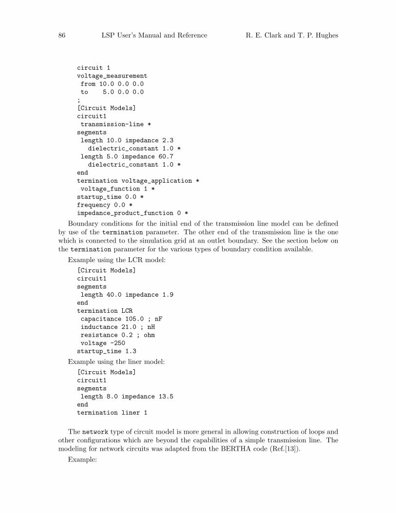
86 LSP User’s Manual and Reference R. E. Clark and T. P. Hughes
circuit 1voltage_measurementfrom 10.0 0.0 0.0to 5.0 0.0 0.0;[Circuit Models]circuit1transmission-line *segmentslength 10.0 impedance 2.3dielectric_constant 1.0 *
length 5.0 impedance 60.7dielectric_constant 1.0 *
endtermination voltage_application *voltage_function 1 *startup_time 0.0 *frequency 0.0 *impedance_product_function 0 *
Boundary conditions for the initial end of the transmission line model can be definedby use of the termination parameter. The other end of the transmission line is the onewhich is connected to the simulation grid at an outlet boundary. See the section below onthe termination parameter for the various types of boundary condition available.
Example using the LCR model:[Circuit Models]circuit1segmentslength 40.0 impedance 1.9endtermination LCRcapacitance 105.0 ; nFinductance 21.0 ; nHresistance 0.2 ; ohmvoltage -250startup_time 1.3
Example using the liner model:[Circuit Models]circuit1segmentslength 8.0 impedance 13.5endtermination liner 1
The network type of circuit model is more general in allowing construction of loops andother configurations which are beyond the capabilities of a simple transmission line. Themodeling for network circuits was adapted from the BERTHA code (Ref.[13]).
Example:

Chapter 6: Input Variables 87
[Circuit Models]circuit1 networkelements1 transit_time 0.1 impedance 0.12 transit_time 1.0 impedance 0.23 transit_time 1.0 impedance 10.04 transit_time 1.36 impedance 1.895 transit_time 0.1 impedance 0.1endjunctionsVOLTAGE_APPLICATION 1voltage 200
RESISTIVE_LOAD 2resistance 1.e9
SERIES_RESISTOR 1 5resistance 0.2
SIMPLE_JUNCTION 2 3PARALLEL_TEE 5 3 4GRID_CONNECTION 4end
The parameters associated with a circuit model are described below.
6.10.1 segments
Specifies the parameters for each section of the transmission line model using the format:segmentslength L1 impedance Z1 dielectric_constant EPS1length L2 impedance Z2 dielectric_constant EPS2...end
where ‘L1’ is the physical length of the segment, ‘Z1’ is the impedance of the segment in userunits (see Chapter 5 [User Units], page 25), and ‘EPS1’ is the relative dielectric constantof the segment. The first segment is the one farthest from the simulation boundary. Thelast segment must have the same impedance as the outlet boundary to which it is attached.The outward-going wave reaching the first segment sees a matched termination unless thetermination parameter specifies some other condition, e.g. SHORT, in which case it seesa short circuit termination. The dielectric_constant parameter is optional and has adefault value of 1.
6.10.2 elements
Specifies the parameters for each element of the network model using the format:elements1 transit_time T1 impedance Z12 transit_time T2 impedance Z23 capacitance C14 inductance L1

88 LSP User’s Manual and Reference R. E. Clark and T. P. Hughes
...end
where ‘T1’ is the transit time of the element and ‘Z1’ is the impedance of the element.Lengths may be used instead of transit times. Note that here each element is numbered foridentification and are not necessarily order dependent, unlike transmission line segmentswhich are order dependent.
Also, for convenience, instead of a characteristic impedance, any element can be indicatedas a lumped capacitor or inductor by using the keywords capacitance or inductance. Ineither case, the transit time keyword and value may be omitted and, if present, are ignoredand treated as zero.
6.10.3 junctions
Defines the configuration of the network, specifying how the elements are linked togetherby using the format:
junctionsRESISTIVE_LOAD 1SIMPLE_JUNCTION 1 2GRID_CONNECTION 2end
which is a list describing the type of junction and identifying the elements, by index number,that are to be associated at these junctions. The junction types available and their definitionare as follows:
VOLTAGE_APPLICATION:An end of an element is a matched termination where a voltage is to be appliedfrom an infinite source. A voltage_function should be supplied in the inputsequence after the element identifier.
RESISTIVE_LOAD:An end of an element is terminated with a resistance. The resistance can beeither a constant value or time-dependent (see below) and is specified after theelement identifier.
SIMPLE_JUNCTION:Two elements with different impedances are joined.
PARALLEL_RESISTOR:Two elements are joined with a resistance between them in parallel. The resis-tance can be either a constant value or time-dependent (see below).
SERIES_RESISTOR:Two elements are joined with a resistance between them in series. The resis-tance can be either a constant value or time-dependent (see below).
PARALLEL_TEE:Three elements are joined such that all three grounds are connected to eachother. Known as a “current adder.”
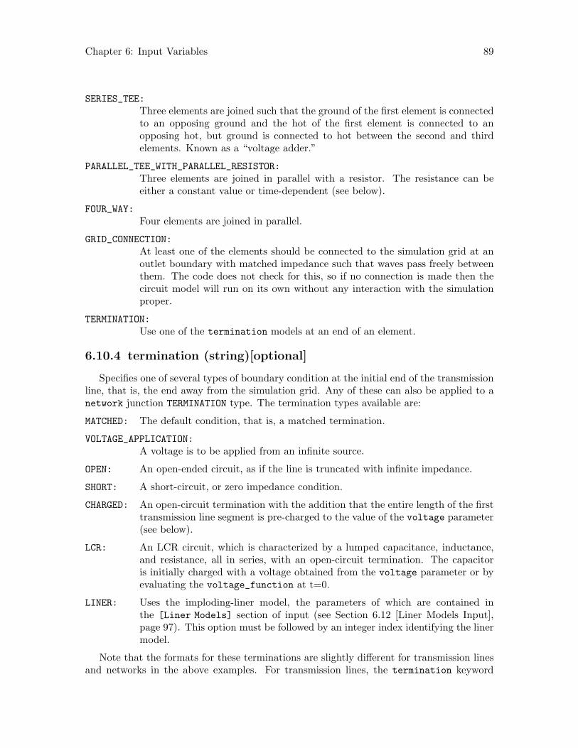
Chapter 6: Input Variables 89
SERIES_TEE:Three elements are joined such that the ground of the first element is connectedto an opposing ground and the hot of the first element is connected to anopposing hot, but ground is connected to hot between the second and thirdelements. Known as a “voltage adder.”
PARALLEL_TEE_WITH_PARALLEL_RESISTOR:Three elements are joined in parallel with a resistor. The resistance can beeither a constant value or time-dependent (see below).
FOUR_WAY:Four elements are joined in parallel.
GRID_CONNECTION:At least one of the elements should be connected to the simulation grid at anoutlet boundary with matched impedance such that waves pass freely betweenthem. The code does not check for this, so if no connection is made then thecircuit model will run on its own without any interaction with the simulationproper.
TERMINATION:Use one of the termination models at an end of an element.
6.10.4 termination (string)[optional]
Specifies one of several types of boundary condition at the initial end of the transmissionline, that is, the end away from the simulation grid. Any of these can also be applied to anetwork junction TERMINATION type. The termination types available are:
MATCHED: The default condition, that is, a matched termination.
VOLTAGE_APPLICATION:A voltage is to be applied from an infinite source.
OPEN: An open-ended circuit, as if the line is truncated with infinite impedance.
SHORT: A short-circuit, or zero impedance condition.
CHARGED: An open-circuit termination with the addition that the entire length of the firsttransmission line segment is pre-charged to the value of the voltage parameter(see below).
LCR: An LCR circuit, which is characterized by a lumped capacitance, inductance,and resistance, all in series, with an open-circuit termination. The capacitoris initially charged with a voltage obtained from the voltage parameter or byevaluating the voltage_function at t=0.
LINER: Uses the imploding-liner model, the parameters of which are contained inthe [Liner Models] section of input (see Section 6.12 [Liner Models Input],page 97). This option must be followed by an integer index identifying the linermodel.
Note that the formats for these terminations are slightly different for transmission linesand networks in the above examples. For transmission lines, the termination keyword

90 LSP User’s Manual and Reference R. E. Clark and T. P. Hughes
and its associated parameters follow the entire sequence of segments, whereas for networks,the termination type and its parameters directly follow the junction with which they areassociated, while omitting the actual termination keyword.
6.10.5 capacitance (real)[optional]
This specifies the capacitance of either the static circuit model, or as part of thetermination LCR option of the transmission-line or network models.
6.10.6 inductance (real)[optional]
This specifies the inductance in the termination LCR option of the transmission-lineor network models.
6.10.7 resistance (real)[optional]
This specifies the resistance of either the static circuit model, or as part of thetermination LCR option of the transmission-line or network models, or any of thenetwork junction types involving a resistance. This parameter can be replaced by aresistance_function, which is explained below.
6.10.8 resistance function (integer)[optional]
This specifies the resistance for any of the network junction types which involve resis-tance as a function of time, that is, it may be used in place of the constant-valued resistanceexplained above. Specifically, when used in conjuction with the SERIES_RESISTOR junctionmodel, it acts as an opening or closing switch by defining the appropriate functional pre-scription in the [Functions] section of input.
6.10.9 voltage (real)[optional]
Value of the voltage for cases in which an initial constant charge is appropriate. Theseare, for example, the static circuit type or either of the “dynamic” models in which aCHARGED or LCR termination is specified.
6.10.10 voltage function (integer)[optional]
Integer index which refers to the function in the [Functions] section specifying thetime-dependence of the inward-going (towards the simulation grid) voltage at the first cir-cuit model element (see Section 6.24 [Functions Input], page 144). This should only beused with the static circuit type, the transmission-line type with the terminationparameter set to VOLTAGE_APPLICATION, CHARGED, or LCR, or the network circuit wherevera junction type is set to VOLTAGE_APPLICATION or TERMINATION where the termination typeis either of CHARGED, LCR, or again, VOLTAGE_APPLICATION. For the static circuit or thetermination LCR case, the function determines only the initial voltage (at t=0) on thecapacitor. If voltage_function is 0, no voltage is applied, and is otherwise ignored whenthe termination parameter is any other kind.

Chapter 6: Input Variables 91
6.10.11 startup time (real)[optional]
Allows the circuit model calculation to be started prior to the main calculation in thesimulation grid; e.g., in a case where the simulation is driven by the circuit model voltage,it may take a significant amount of time for a nonzero voltage to reach the simulationboundary. The units for time are dependent upon which system of units has been specifiedby the user (see Chapter 5 [User Units], page 25), but the number should be positive. Theuser must insure that the actual transit time for the sum of the element lengths specified isnot exceeded.
6.10.12 frequency (real)[optional]
Specifies the incoming wave frequency in Hz. The amplitude is determined by eitherthe voltage parameter or the voltage_function parameter below, depending on which isspecified.
6.10.13 impedance product function (integer)[optional]
Index of a function in the [Functions] section which specifies a time-varying multiplierapplied to the impedance of the first element of the circuit model (see Section 6.24 [FunctionsInput], page 144). However, the resulting impedance mismatch affects only the outgoingwave, not the incoming voltage pulse. If impedance_product_function is 0, no multiplieris applied.

92 LSP User’s Manual and Reference R. E. Clark and T. P. Hughes
6.11 Volume Models Input
The [Volume Models] section of the input file provides a number of models which canbe applied over grid-conformal blocks of the simulation space. Entries in this section arenumbered consecutively by appending an integer index to the volume keyword. Most ofthese models are intended to be used only with dynamic field solution, rather than staticfield solution. The dielectric model is the only volume model that can be invoked whileusing a static field solver. The models currently available are described below.
Examples are:[Volume Models]volume1dipole Zfrom 2.0, 0.0, 12.5to 2.0, 0.2618, 13.0total_current 2.5e5 ; ampstemporal_function 2 *secondary_function 3 *spatial_function 0 *reference_point 0 0 0 *spatial_flags 0 0 0 *
volume2conductivity Zfrom 2.0 0.0 1.0to 2.0 0.5 4.0sigma 10.0temporal_function 0 *
volume3ferritefrom 0.5 0.9 0.0to 0.9 2.0 10.0permeability 285.0 8.0 ; static and infinite valuesresonancessine_coefficient 0.0 cosine_coefficient 5.21e10decay_rate 1.88e8 frequency 0.0end
When it is necessary to construct a repetitive series of similar volume models, it ispossible to use additional instructions after a single instance that repeats the model anumber of times, translated by some constant distance in succession. The format is:
repeat N times, with X Y Z
where ‘N’ is the number of additional volumes generated and ‘X Y Z’ is the spatial translationvector to be used each time.
Example:volume1dielectricfrom 0.0 0.0 0.0
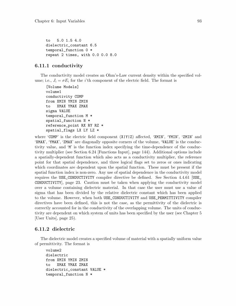
Chapter 6: Input Variables 93
to 5.0 1.5 4.0dielectric_constant 6.5temporal_function 0 *repeat 2 times, with 0.0 0.0 8.0
6.11.1 conductivity
The conductivity model creates an Ohm’s-Law current density within the specified vol-ume; i.e., Ji = σEi for the i ’th component of the electric field. The format is
[Volume Models]volume1conductivity COMPfrom XMIN YMIN ZMINto XMAX YMAX ZMAXsigma VALUEtemporal_function M *spatial_function N *reference_point RX RY RZ *spatial_flags LX LY LZ *
where ‘COMP’ is the electric field component (X|Y|Z) affected, ‘XMIN’, ‘YMIN’, ‘ZMIN’ and‘XMAX’, ‘YMAX’, ‘ZMAX’ are diagonally opposite corners of the volume, ‘VALUE’ is the conduc-tivity value, and ‘M’ is the function index specifying the time-dependence of the conduc-tivity multiplier (see Section 6.24 [Functions Input], page 144). Additional options includea spatially-dependent function which also acts as a conductivity multiplier, the referencepoint for that spatial dependence, and three logical flags set to zeros or ones indicatingwhich coordinates are dependent upon the spatial function. These must be present if thespatial function index is non-zero. Any use of spatial dependence in the conductivity modelrequires the USE_CONDUCTIVITY compiler directive be defined. See Section 4.4.61 [USE_CONDUCTIVITY], page 23. Caution must be taken when applying the conductivity modelover a volume containing dielectric material. In that case the user must use a value ofsigma that has been divided by the relative dielectric constant which has been appliedto the volume. However, when both USE_CONDUCTIVITY and USE_PERMITTIVITY compilerdirectives have been defined, this is not the case, as the permittivity of the dielectric iscorrectly accounted for in the conductivity of the overlapping volume. The units of conduc-tivity are dependent on which system of units has been specified by the user (see Chapter 5[User Units], page 25).
6.11.2 dielectric
The dielectric model creates a specified volume of material with a spatially uniform valueof permittivity. The format is
volume2dielectricfrom XMIN YMIN ZMINto XMAX YMAX ZMAXdielectric_constant VALUE *temporal_function N *

94 LSP User’s Manual and Reference R. E. Clark and T. P. Hughes
where ‘XMIN’, ‘YMIN’, ‘ZMIN’, ‘XMAX’, ‘YMAX’, ‘ZMAX’ are diagonally opposite corners of thevolume, ‘VALUE’ is the relative dielectric constant, and ‘N’ is the function index specifyingthe time-dependence of the dielectric value multiplier (see Section 6.24 [Functions Input],page 144).
When using this model with the ADI field solver (see Section 4.4.30 [IMPLICIT_FIELDS],page 19), the compiler directive USE_PERMITTIVITY must be defined. See Section 4.4.64[USE_PERMITTIVITY], page 23.
A more general way to specify dielectric materials is through a medium model associatedwith structural objects (see Section 6.5 [Objects Input], page 56).
6.11.3 dipole
The dipole model places an externally-applied current density within the specified vol-ume. The format is
volume1dipole COMPfrom XMIN YMIN ZMINto XMAX YMAX ZMAXtotal_current VALUEtemporal_function M *secondary_function S *spatial_function N *reference_point RX RY RZ *spatial_flags LX LY LZ *
where ‘COMP’ is the component direction of the current density (X|Y|Z), ‘XMIN’, ‘YMIN’,‘ZMIN’, ‘XMAX’, ‘YMAX’, ‘ZMAX’ are diagonally opposite corners of the volume, ‘VALUE’ is thetotal current value, and ‘M’ is the function index specifying the time-dependence of thecurrent multiplier, if present (see Section 6.24 [Functions Input], page 144). Additionaloptions include specification of a secondary temporal function (which results in a productfunction with the primary temporal function), a spatially-dependent function which alsoacts as a current multiplier, the reference point for that spatial dependence, and threelogical flags set to zeros or ones indicating which coordinates are dependent upon the spatialfunction. These must be present if the spatial function index is non-zero.
6.11.4 ferrite
The ferrite model creates a linear dispersive magnetic material in the specified volume.The “recursive-convolution” method (Ref.[11]) is used to perform the necessary convolutionin an efficient manner. The general form of the response function is:
B(t) = µ∞H(t) + χ(t) ∗H(t)
where the ∗ denotes convolution, and χ(t) is written as
χ(t) =N∑
i=1
[Ai sin(ωit) + Bi cos(ωit)]e−δit

Chapter 6: Input Variables 95
Usually, the response function is approximated by a sum of single-pole Debye relaxationsand double-pole Lorentzian resonances. For a Debye relaxation, χ(t) takes the form
χ(t) = (µs − µ∞)δie−δit
so that ω = 0, Ai = 0, Bi = (µs − µ∞)δi. The values µs, µω give the zero- and infinite-frequency limits of the permeability, respectively.
The ferrite model cannot be used with the ADI field solver (see Section 4.4.30 [IMPLICIT_FIELDS], page 19).
The format is:
volume1ferritefrom XMIN YMIN ZMINto XMAX YMAX ZMAXpermeability MU_STATIC MU_INFresonancessine_coefficient S1 cosine_coefficient C1decay_rate DELTA1 frequency FREQ1sine_coefficient S2 cosine_coefficient C2decay_rate DELTA2 frequency FREQ2...end
where ‘XMIN’, ‘YMIN’, ‘ZMIN’, ‘XMAX’, ‘YMAX’, ‘ZMAX’ are diagonally opposite corners of thevolume, ‘MU_STATIC’ is the limiting value of the magnetic permeability for zero frequency,‘MU_INF’ is the limiting value of the magnetic permeability for infinite frequency, ‘S1’ and‘C1’ are the coefficients in the representation of the response function and ‘FREQ1’, ‘DELTA1’are the resonant frequency (in rads/sec) and decay rate (1/sec) of the first resonance. Upto MAX_RESONANCES (see Section 4.4.39 [MAX_RESONANCES], page 20) relaxations/resonancescan be specified between the resonances and end keywords.
6.11.5 hysteresis
The magnetic hysteresis model utilizes both magnetic induction and magnetic intensityin the cells in order to model magnetic hysteresis phenomena. The format is
volume1hysteresisfrom XMIN YMIN ZMINto XMAX YMAX ZMAXdata_file FILE
where ‘XMIN’, ‘YMIN’, ‘ZMIN’, ‘XMAX’, ‘YMAX’, ‘ZMAX’ are diagonally opposite corners of thevolume and ‘FILE’ is the name of the data file containing a series of B-H hysteresis curves.The format for this file is defined in the section under “File Formats” in Section 7.12[Hysteresis Data File], page 163.
When using this model, the compiler directive MAGNETIC_HYSTERESIS must be defined.See Section 4.4.36 [MAGNETIC_HYSTERESIS], page 20. In addition, the B and H magnetic
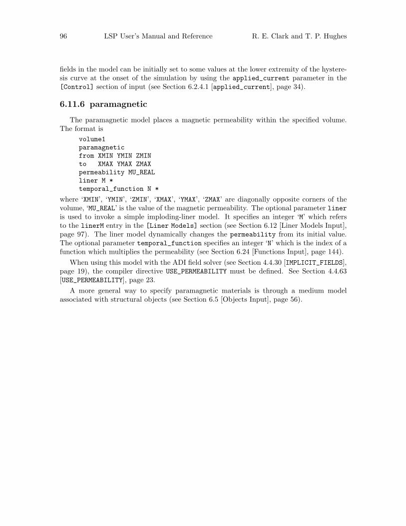
96 LSP User’s Manual and Reference R. E. Clark and T. P. Hughes
fields in the model can be initially set to some values at the lower extremity of the hystere-sis curve at the onset of the simulation by using the applied_current parameter in the[Control] section of input (see Section 6.2.4.1 [applied_current], page 34).
6.11.6 paramagnetic
The paramagnetic model places a magnetic permeability within the specified volume.The format is
volume1paramagneticfrom XMIN YMIN ZMINto XMAX YMAX ZMAXpermeability MU_REALliner M *temporal_function N *
where ‘XMIN’, ‘YMIN’, ‘ZMIN’, ‘XMAX’, ‘YMAX’, ‘ZMAX’ are diagonally opposite corners of thevolume, ‘MU_REAL’ is the value of the magnetic permeability. The optional parameter lineris used to invoke a simple imploding-liner model. It specifies an integer ‘M’ which refersto the linerM entry in the [Liner Models] section (see Section 6.12 [Liner Models Input],page 97). The liner model dynamically changes the permeability from its initial value.The optional parameter temporal_function specifies an integer ‘N’ which is the index of afunction which multiplies the permeability (see Section 6.24 [Functions Input], page 144).
When using this model with the ADI field solver (see Section 4.4.30 [IMPLICIT_FIELDS],page 19), the compiler directive USE_PERMEABILITY must be defined. See Section 4.4.63[USE_PERMEABILITY], page 23.
A more general way to specify paramagnetic materials is through a medium modelassociated with structural objects (see Section 6.5 [Objects Input], page 56).
Chapter 6: Input Variables 97
6.12 Liner Models Input
The [Liner Models] section of the input file specifies parameters for a simple imploding-liner model. Entries in this section are numbered consecutively by appending an integerindex to the liner keyword. This integer may be used in the paramagnetic model to obtaina dynamically changing magnetic permeability over a specified volume (see Section 6.11.6[paramagnetic], page 96). This allows a self-consistent treatment of the changing induc-tance of the liner region. The user must ensure that the liner dimensions are consistentwith the actual geometry.
The format is:[Liner Models]liner1mass Mlength Louter_radius ROinner_radius RIfinal_radius RF
where ‘M’ is the mass of the liner, ‘L’ is the length of the liner, ‘RO’ is the outer radius ofthe can containing the liner, ‘RI’ is the initial inner radius of the liner, and ‘RF’ is the finalradius of the liner after implosion. Note that RF is smaller than RI, causing the impedanceto increase as the liner implodes.

98 LSP User’s Manual and Reference R. E. Clark and T. P. Hughes
6.13 Subgrid Models Input
The [Subgrid Models] section of the input file provides a means of modeling structureelectromagnetically on scales which are smaller than the gridding provides; for example asmooth non-conformal surface which cannot be accomplished with ordinary stair-steppingtechniques. This is an idea taken from Jurgens et al. (Ref.[8]), where it was used inscattering simulations on spherical bodies in a 3-D cartesian mesh.
At present, the only use of this technique is for a flat surface sloped in any two coordinatedirections, but not all three. This model, although it is useful for eliminating undesirablewave distortion which may result from a stair-stepped model, is not suitable for particlecharge conservation, and should only be used in areas of the simulation where particles donot occur. Also, it has not yet been implemented for static fields solutions or implicit fieldssolutions. When using this model, the compiler directive USE_SUBCELLS must be defined.See Section 4.4.66 [USE_SUBCELLS], page 23.
Example:[Subgrid Models]subgrid1 SLOPE ; pierce electrodenormal0 Znormal1 -Xfrom 8.25 0 13.0to 17.25 0 17.0
where the two normal parameters control the orientation and the from to coordinatesmerely indicate the space in which the model is located. These are not necessarily thetwo end-points of the slope. The actual orientation is determined by the normal parameterswhich are understood to give the signed direction normal to the conducting surface. Theuser does not ordinarily place any other structural objects explicitly within the coordinateboundaries indicated by the subgrid model (see Section 6.5 [Objects Input], page 56).

Chapter 6: Input Variables 99
6.14 Substrate Models Input
The [Substrate Models] section of the input file provides a means of emitting ionspecies which exist as absorbed material in a specially prepared metal plate. Entries inthis section are numbered consecutively by appending an integer index to the substratekeyword. The only model currently available is described below. Note that the numberof materials is three. The first material is the metallic plate; the second is the ceramicbacking; the third is an aluminum oxide sleeve. The production of ions from the substrateis stimulated by energy deposition on the surface. Therefore, the substrate model must beimbedded in a structural surface of conductor material in order to function correctly. Thismodel may not be available in all releases of the LSP code.
Example:[Particle Species]species2 ; Hydrogencharge 0mass 1837.0
[Substrate Models]; Hydrogen source - materials: Metal, Ceramic, Aluminumsubstrate1atomic_weight_of_metallic_layer 45.0densities_of_materials 3.00 5.53 3.80 ; g/ccradii_of_materials 0.1 0.07 0.2depth_of_metallic_layer 6.0e-1depth_of_ceramic_layer 14.0e-1radial_resolution 50axial_resolution 50initial_temperature 300.0 ; kelvinratio_H_to_M 1.0 ; ratio of absorbed hydrogen to metal ionsreference_point 0. 0. 5.0alignment_axis -Zinterval 10species 2 *minimum_charge 0.0 *movie_tag 0 *movie_fraction 0.0 *

100 LSP User’s Manual and Reference R. E. Clark and T. P. Hughes
6.15 External Fields Input
External fields are user-prescribed fields which are added to the self-consistent electro-magnetic fields produced by the simulation, exclusively for the purpose of affecting particleforces. Single values, 1-D arrays, 2-D arrays, and 3-D arrays of electric or magnetic fieldscan be used. For 1-D arrays the field values are described by an input function as describedbelow. For 2-D and 3-D arrays the field values are read from user-supplied data files. Thecoordinate values for the external fields on these files need not match the LSP simulationgrid, as they are interpolated onto it.
For 2-D field arrays, the data file contains cylindrical Bz, Br data. Two formats aresupported: one produced by the BFIELD code which can be in either ASCII text or binaryform (see Section 7.4 [BFIELD Magnetic Field File], page 159), and an ASCII text fileproduced by the SNL ATHETA code (see Section 7.5 [ATHETA Magnetic Field File],page 160). In both cases, the data are transformed into Bx, By, Bz when using a cartesiansimulation grid.
For 3-D fields, an ASCII file produced by the MAG3D code can be accepted (see Sec-tion 7.6 [MAG3D Magnetic Field File], page 160), or a similar binary file produced byMAFCO may be utilized (see Section 7.7 [MAFCO Magnetic Field File], page 161). Thelatter file type is produced by the mafco code contained internally in the LSP package.
The parameters associated with external field input are described below.Example of single-value input:
[External Fields]external1type COMPONENTfield B Z 300.0temporal_function 0 *
where the qualifier COMPONENT indicates the single-value option.Example of 1-D array input:
[External Fields]external1type ANALYTICfield B Zspatial_function 1from 0.0 0.0 0.0 *to 8.0 8.0 8.0 *reference_point 0.0 0.0 0.0 *alignment_axis Z *symmetry_direction NONE *temporal_function 0 *;[Functions]; external field data for the laser diodefunction1type 0data_pairs-6.00E+00 6.7315E+02-4.30E+00 7.1863E+02

Chapter 6: Input Variables 101
-2.60E+00 7.6390E+02-9.00E-01 8.0763E+028.00E-01 8.4832E+022.50E+00 8.8445E+024.20E+00 9.1476E+025.90E+00 9.3843E+02
end
Example of 1-D array input with bilateral symmetry:[External Fields]external1type ANALYTICfield B Zspatial_function 1reference_point 0.0 0.0 0.0 *alignment_axis Z *symmetry_direction Y *temporal_function 0 *
Example of 1-D array input with axial symmetry:[External Fields]external1type ANALYTICfield B Zspatial_function 1reference_point 0.0 0.0 0.0 *alignment_axis Z *symmetry_direction THETA *order 6 *temporal_function 0 *
Example of data file input:[External Fields]external1type DATAFILE FILETYPE FILENAMEformat binary *reference_point 0.0 0.0 50.0 *alignment_axis Z *temporal_function 0 *
6.15.1 type (string)
Specifies the type of external fields input. It can take the values COMPONENT for a singlevalue, ANALYTIC for a 1-D array of field values, or DATAFILE for a 2-D or 3-D array of valuessupplied in an external file.
For the ANALYTIC option, the 1-D array is a tabulated function (see Section 6.24 [Func-tions Input], page 144) specified by the spatial_function parameter. The first column ofthe table gives the spatial coordinate and the second gives the magnetic field.
For the DATAFILE option, which indicates 2- or 3-dimensional data con-tained on a user-supplied file, FILETYPE specifies one of the available file types

102 LSP User’s Manual and Reference R. E. Clark and T. P. Hughes
(BFIELD|ATHETA|MAG3D|MAFCO), and FILENAME is the name of the file supplied by the user.An explanation of the various file types is explained in the section on File Formats. (SeeChapter 7 [File Formats], page 157.)
For the ANALYTIC and DATAFILE options, either one or both of the compiler directivesEXTERNAL_BFIELDS or EXTERNAL_EFIELDS must be defined at compilation time, dependingon which of those fields are indicated by the field parameter described below (see Sec-tion 4.4.22 [EXTERNAL_BFIELDS], page 17, see Section 4.4.23 [EXTERNAL_EFIELDS], page 18).Also, note that the use of multiple instances of either of these types (of the same field)requires that the definition of EXTERNAL BFIELDS or EXTERNAL EFIELDS is set tothe number of instances requested on input.
6.15.2 field (string)
Specifies an external magnetic or electric field (B|E). The format for this parameterwhen the COMPONENT option is in effect is
field B X|Y|Z VALUE
which specifies the value ‘VALUE’ for the X|Y|Z component of the external magnetic field,or,
field E X|Y|Z VALUE
which specifies the value ‘VALUE’ for the X|Y|Z component of the external electric field.
For the ANALYTIC option, a ‘VALUE’ does not appear.
For the DATAFILE option, this parameter need not appear since all of the file optionsinvolve only magnetic fields.
where ‘FILENAME’ is the name of the datafile. The various file formats are given in Chapter 7[File Formats], page 157. For the BFIELD specification, the optional keyword FORMAT maybe present to indicate that the file is either type ASCII or binary with ASCII being thedefault.
6.15.3 format (string)[optional]
Format for data file to be read - ASCII or binary.
Default: ASCII
6.15.4 from to (real)[optional]
The parameters from, to, specify the lower and upper coordinate limits of the volumeover which the field is applied. They are optional, and if not specified, the field is appliedeverywhere. These parameters are ignored for the simple COMPONENT type.
6.15.5 reference point (real)[optional]
The origin for the external field is shifted to the coordinates of reference_point on thesimulation grid.
Chapter 6: Input Variables 103
6.15.6 alignment axis (string)[optional]
For a 1-D external field, specifies the direction (X|Y|Z) of the spatial coordinate in thefield data, and the field component. For a 2-D external field, specifies the direction inthe simulation grid (X|Y|Z) corresponding to the Z direction in the field data file. Thisparameter has no effect for 3-D data contained in the MAG3D or MAFCO formats under theDATAFILE option.
Default: Z
6.15.7 symmetry direction (string)[optional]
For the ANALYTIC option only, the transverse components of the magnetic field are cal-culated analytically according to which option is specified:
symmetry_direction DIR
where ‘DIR’ can have the values NONE|X|Y|Z|THETA. The value NONE indicates that notransverse components are calculated. Use of the THETA option produces an analytic ex-pansion for the off-axis cylindrically symmetric fields, based upon the axial field specifiedin the spatial_function. Use of one of the X|Y|Z tokens will result in a single componentof transverse field being calculated. Note that this component should not be the same asthe main component given by the alignment_axis parameter.
Default: NONE
6.15.8 order (integer)[optional]
For the THETA option of the symmetry_direction parameter only, the order parameterindicates the order of the expansion used in the evaluation of the transverse dependencefor axial symmetry. The value used should not exceed 6. Generally, use of higher ordersrequires more highly resolved and accurate data in the spatial_function.
Default: 2
6.15.9 temporal function (integer)[optional]
Integer identifying the time-dependent function used to multiply the external fieldvalue(s). For the COMPONENT option, there are no restrictions in the use of this parameterwhen multiple instances of external field are required. However, with the more complexdescriptions, designated by the ANALYTIC and DATAFILE options, use of multiple instancesof either of these types (of the same field) are restricted to a single temporal dependencegiven by this parameter in the first instance. For no time-dependence, set the value to 0.(See Section 6.24 [Functions Input], page 144.)

104 LSP User’s Manual and Reference R. E. Clark and T. P. Hughes
6.16 Particle Species Input
The [Particle Species] section specifies the particle species to be used in the sim-ulation and their properties. Each species is identified by the integer index appended tothe species keyword. This integer is used elsewhere in the input file to refer to thatspecies. If ionization (see Section 6.17.10 [ionization], page 122) or photoionization (seeSection 6.17.12 [photoionization], page 124) is being used, then each ionization state istreated as a separate species, and successively higher ionization states must be listed insequence (i.e., if species3 is neutral, then the first ionization state should be species4,etc.)
The parameters for the species are described below.Example:
[Particle Species]species1charge -1mass 1.0fluid_species_flag off *migrant_species_flag off *implicit_species_flag off *particle_motion_flag on *particle_forces_option averaged *transverse_weighting_flag on *particle_kinematics_option standard *montecarlo_scattering_flag off *selection_ratio 0.5 *species2charge +1mass 1836.0atomic_number 1 *selection_ratio 1.0 *
Example when using the ionization model (see Section 6.17.10 [ionization], page 122):[Particle Species]species1charge -1mass 1.0fluid_species_flag off *particle_forces_option primary *species2charge +1mass 1836.0atomic_number 1 *species3charge 0mass 3674.0atomic_number 2 *species4charge +1mass 3673.0
Chapter 6: Input Variables 105
atomic_number 2 *
Example when using the higherstate model (see Section 6.17.11 [higherstate],page 123):
[Particle Species]species1charge -1mass 1.0fluid_species_flag off *particle_forces_option averaged *; Nitrogen ionsspecies2charge +1mass 27540.0atomic_number 7 *species3charge +2mass 27539.0atomic_number 7 *
Example of implicit species:[Particle Species]species1charge -1mass 1.0implicit_species_flag on *particle_motion_flag on *particle_forces_option primary *montecarlo_scattering_flag on *implicit_filtering_parameter 1.0 *selection_ratio 0.2 *
6.16.1 charge (real)
Gives the charge state for each species, normalized to that for a positron. Thus, anelectron is -1, and a proton is +1 (plus-sign optional) and a neutral is 0.
6.16.2 mass (real)
Gives the mass for each species, normalized to that for a positron. Thus, an electron is1, and a proton is 1836.
6.16.3 atomic number (real)[optional]
Atomic number of ion species. Used with the ionization model (see Sec-tion 6.17.10 [ionization], page 122), the photoionization model (see Section 6.17.12[photoionization], page 124), or with the higherstate model (see Section 6.17.11[higherstate], page 123), that is, any particle creation model which involves the transitioninto a higher charge state (ionization or stripping).
106 LSP User’s Manual and Reference R. E. Clark and T. P. Hughes
6.16.4 fluid species flag (flag)[optional]
Indicates which charged-particle species are treated as fluid particles when the fluidphysics (see Section 4.4.25 [FLUID_PHYSICS], page 18) portion of the collisional plasmascattering model (see Section 4.4.48 [SCATTERING_ON], page 21) has been invoked. Thisoption is particularly useful in the direct-implicit algorithm when the product of the speciesplasma frequency and timestep is large. Numerical cooling will occur in this case if thespecies is treated kineticly.
Default: OFF
6.16.5 migrant species flag (flag)[optional]
Indicates which electron species are treated as “migrating” species for the hybrid plasmamigration model, which is an optional feature of the fluid physics portion of the collisionalplasma scattering model. Only particles which belong to a species which has been designatedas a migrant species have the ability to transform into one of the opposite type. Thatis, kinetic type electrons become fluid electron species, and vice-versa. This process isdescribed in the Particle Migration section of input (see Section 6.19 [Particle MigrationInput], page 135).
Default: ON
6.16.6 implicit species flag (flag)[optional]
Indicates which species undergo implicit advancement in the particle kinematics. TheDIRECT_IMPLICIT compiler directive must be defined in order for this option to be relevant(see Section 4.4.16 [DIRECT_IMPLICIT], page 16).
Default: ON
6.16.7 particle motion flag (flag)[optional]
For species with particle_motion_flag set to OFF, the particle positions never change.This may be useful for analysis of pure scattering phenomena.
Default: ON
6.16.8 particle forces option (string)[optional]
Selects the method by which the fields effect particle forces. The option AVERAGEDwill cause the spatially averaged fields at grid node positions to be used. The optionPRIMARY or STAGGERED will use the fields directly calculated from the E-M solution on theparticles. Additionally, the particle_forces_option can be set to NONE, in which case,the particle positions will be advanced but not their momenta. The AVERAGED option isgood for momentum conservation, in that there are no “self forces” on the particles. ThePRIMARY option produces an energy-conserving push that is not susceptible to the so calledDebye-length numerical instability. The simulation is numerically stable even for grid sizelarger than the plasma skin depth, although resolution of this parameter is desirable. Themagnetic field in this case is still provided by the averaged values as for the AVERAGED option.The PRIMARY option is recommended (and is the default) when the EXTENDED_PARTICLES
Chapter 6: Input Variables 107
compiler directive has been defined (see Section 4.4.21 [EXTENDED_PARTICLES], page 17).This choice is required for species that have been designated for implicit advancement.
Default: AVERAGED for explicit species, PRIMARY for implicit species or when EXTENDED_PARTICLES is defined.
6.16.8.1 transverse weighting flag (flag)[optional]
Used to modify the spatial weighting scheme for particle forces due to fields. This canbe set to OFF under simulation conditions where a continuous beam would produce a “saw-tooth” instability. Ordinarily, this flag is left ON. This flag applies to explicit species only,and is ignored for implicit species. Also, this flag is ignored if the EXTENDED_PARTICLEScompiler directive is defined and the particle_forces_option is set to PRIMARY.
Default: ON
6.16.9 particle kinematics option (string)[optional]
Used for the selection of multiple options in the method of advancing particle momentum.The STANDARD option uses the familiar “leap-frog” technique with the magnetic field rotationsplitting the electric field push into two separate halves. The IMPLICIT option does theelectric and magnetic advancements simultaneously. The PARAXIAL option is a simplifiedcalculation appropriate only for paraxial beams. This parameter applies to explicit speciesonly, and is ignored for implicit species.
Default: STANDARD
6.16.10 montecarlo scattering flag (flag)[optional]
Indicates which species (usually electrons) undergo random montecarlo scattering in thecollisional plasma model. If this is set to OFF, the scattering is done in an averaged wayand results in an energy distribution that is not as accurate. In order to use this option,the appropriate interaction file must be provided in the [Particle Interaction] sectionof input (see Section 6.21 [Particle Interaction Input], page 138). The SCATTERING_ONcompiler directive must be defined in order for this option to be relevant (see Section 4.4.48[SCATTERING_ON], page 21).
Default: OFF
6.16.11 implicit filtering parameter (real)[optional]
Damping factor for the “c0-d1” particle push (Ref.[3]). The default value is 1, givingmaximum damping (d1 scheme). A value of 0 gives the undamped, reversible c0 scheme.This parameter applies to implicit species only.
Default: 1 (maximum damping - d1 scheme)
6.16.12 selection ratio (integer)[optional]
Causes a random selection of particles of this species during output of the particle dumpssuch that the number selected is a fraction of the total according to this ratio.
Default: 1.0

108 LSP User’s Manual and Reference R. E. Clark and T. P. Hughes
6.17 Particle Creation Input
Particles can be introduced into the simulation in several ways. The following table liststhe keywords used to invoke the available models:
emission:emission from a surface, using either the child-langmuir, field-limited,source-limited or stimulated models discussed below
injection:injection through a boundary (e.g., a beam)
secondary:secondary emission of electrons and positrons from a surface as a result of eithera method 2 medium or a method 4 medium (see Section 6.9 [Medium ModelsInput], page 73)
backscatter:backscatter is applied to particles, primary or secondary, which have impingedupon a method 3 medium (see Section 6.9 [Medium Models Input], page 73)
desorption:thermal and/or stimulated desorption of neutrals and ions from a surface
ionization:collisional ionization, usually applied to neutral ion species (charge 0)
higherstate:currently this is a specialized ion-ion stripping model
photoionization:ionization of neutral or charged species by photons
plasma: plasma existing in the simulation space at the start of the simulation
excitation:conversion of electrons from a low energy state to an excited state by laseracceleration
fragmentation:conversion of heavier molecules into smaller ones by bond breaking
fileread:injection using particle data from a previously created file
fission: numerical particle splitting in regions where the physics is hampered by thecoarseness of particle statistics (e.g., emission from the surface of a denseplasma)
trajectory:tracer particles which produce an output file giving their trajectory and thefields acting on them.
All of these models are invoked from the [Particle Creation] section of the inputfile. The following sections describe generic and model-specific parameters for the models.Sample models follow the first section.
Chapter 6: Input Variables 109
6.17.1 Particle Creation Parameters
Parameters which are common to more than one model are described in the followingsections.
6.17.1.1 from to (real)
The parameters from, to, specify the lower and upper limits of the area or volume overwhich the creation model is applied. See the sections on the individual models to determinehow to use these parameters.
6.17.1.2 normal (string)
Specifies a particle direction (e.g., injection, fileread). Can take the values X, -X, Y,-Y, Z, -Z.
6.17.1.3 interval (integer)
Number of timesteps between application of particle-creation model.
6.17.1.4 species (integer)
Integer identifying species to be created, or for any of the stripping models, the specieswhich is acted upon to create the next higher ionized state. These last are the ionization,higherstate, and photoionization models. In such cases, the identified species on theParticle Species Input list must be followed by a species corresponding to its next higherstate, that is, with a charge greater by 1 and with a mass which is smaller by 1. (SeeSection 6.16 [Particle Species Input], page 104.)
6.17.1.5 electron species (integer)
Integer identifying the species to which the newly created electron produced in an ion-ization event belongs. The electrons may be either of kinetic or fluid type (provided thecompiler directive FLUID_PHYSICS is defined). (See Section 6.16 [Particle Species Input],page 104.)
6.17.1.6 discrete numbers (integer)[optional]
For the emission, injection and plasma models, this specifies the number of particlesper cell in the X|Y|Z directions, respectively. The value in the direction of injection oremission is usually 1. Two numbers may be entered in the case of 2D simulations and areunderstood to correspond to the actual dimensions used. This input item defaults to asingle particle per cell.
Default: 1 1 1
110 LSP User’s Manual and Reference R. E. Clark and T. P. Hughes
6.17.1.7 centroid1&2 function (integer) [optional]
Integers identifying the functions (centroid1_function and centroid2_function)used to specify the time-dependence of the injected beam centroid position in the twodirections transverse to the injection direction, relative to the reference_point below.The two directions are in cyclic order (X, Y, Z) with the injection direction. However,for cylindrical coordinates, where the injection direction is Z, the transverse directionsfor these functions are understood to be in a cartesian sense, that is, X and Y. Theseparameters are optional and may be omitted (or set to zero) if there is no centroid motion.See Section 6.24 [Functions Input], page 144.
6.17.1.8 reference point (real)
The origin for particle coordinates is shifted to the coordinates of reference_point onthe simulation grid. The number of values which follow this parameter may correspond tothe actual number of dimensions defined for the simulation (1, 2, or 3), although all threevalues may be present when a reduced number of dimensions is used.
6.17.1.9 drift momentum (real)
Specifies constant momentum values in the X, Y, Z directions which are applied to ev-ery particle in units of gamma-beta. This parameter conflicts with the drift_velocityparameter and they should not both appear in the same instance of a Particle CreationInput.
6.17.1.10 drift velocity (real)
Specifies constant velocity values in the X, Y, Z directions which are applied to everyparticle in user units (length/time). This parameter conflicts with the drift_momentumparameter and they should not both appear in the same instance of a Particle CreationInput.
6.17.1.11 random (flag)
If ON, randomize the particle initial position within the cell where it is created.
6.17.1.12 medium (integer)[optional]
Specifies a medium index for which the model is applied; that is, only those cells whichcontain that specific medium identifier will participate in the process associated with themodel. The parameter appears in this form for the emission and desorption models.When it is not used or set to 0, it is ignored and all cells within the defined volume willparticipate. Note that other particle creation models may contain medium identifiers whichare mandatory, in which case they are listed in their appropriate Particle Creation Inputsubsections.
6.17.1.13 charge factor (real)[optional]
A multiplier applied to the emitted charge after it has been calculated from the appro-priate model. This can be used to suppress particle creation when desirable.
Chapter 6: Input Variables 111
6.17.1.14 thermal energy (real)[optional]
Thermal energy (in eV) used to add a Gaussian distribution to the momentum or to setthe temperature in the case of a fluid species.
Default: 0.0
6.17.1.15 slice times (integer)[optional]
A list of times (in user units) at which injected particles (from either the injection orfileread models) are tagged for particle-slice diagnostics (see Section 6.25.4 [Particle-SliceProbes], page 153).
6.17.1.16 movie tag (integer)[optional]
Integer (0 < movie_tag < 8) used to identify the particles created with the current modelin the movie file. (See Section 1.3 [P4 Postprocessor], page 3.)
Default: 0 (no tag)
6.17.1.17 movie fraction (real)[optional]
Fraction of particles created which will be tagged for output to the movie file. (SeeSection 1.3 [P4 Postprocessor], page 3.)
Default: 0.0 (no particles tagged)
6.17.2 emission (child-langmuir)
Child-Langmuir emission is the standard space-charge-limited emission model. Thereare two sub-models which differ only in the method used to determine the onset of emis-sion. These are the field-stress and thermal breakdown methods (see Section 6.17.2.3[threshold (emission)], page 113). Use of the thermal breakdown method requires that thecompiler directive KELVIN_DEPOSITION be defined (see Section 4.4.33 [KELVIN_DEPOSITION],page 19). Model-specific parameters are described below. Generic parameters are describedin Section 6.17.1 [Particle Creation Parameters], page 109.
Example of Child-Langmuir emission:emission child-langmuir field-stressfrom 6.9, 0.0, 0.8to 7.35, 6.283, 1.95interval 2species 1discrete_numbers 1 1 1 *random offmedium 0 *inclusion vacuum *threshold 25.55 *charge_factor 1.0 *surface_factor 0.66667 *thermal_energy 0.0 *movie_tag 1 *
112 LSP User’s Manual and Reference R. E. Clark and T. P. Hughes
movie_fraction 0.2 *
Example of Child-Langmuir emission with temporal dependence for breakdown:
emission child-langmuir field-stressfrom 1.0, 0.0, 1.0to 1.5, 3.0, 1.5interval 1species 1random offmedium 0 *threshold 25 *breakdown_function 1 *surface_factor 1.0 *thermal_energy 0.0 *movie_tag 0 *movie_fraction 0.0 *
Example of Child-Langmuir emission with thermal breakdown:
emission child-langmuir thermalfrom 0.0, 0.0, 0.0to 5.0, 5.0, 2.5interval 1species 1random offmedium 1 *threshold 400 *surface_factor 1.0 *thermal_energy 0.0 *movie_tag 0 *movie_fraction 0.0 *
6.17.2.1 from to (real)
These coordinate parameters describe a volume of the simulation space over which themodel is applied. The test cells within this volume which can cause emission are solidsurface cells (conductor or dielectric) or adjoining vacuum cells, depending upon the methodspecified for the inclusion parameter below. In either case, particles can only be createdat surface interfaces between solid cells and vacuum cells.
6.17.2.2 inclusion (string)[optional]
This parameter prescribes the rule that determines which cell surfaces are emitters withinthe from to range described above. The possible values are either SOLID or VACUUM, suchthat only cells of those types within the specified coordinates become candidates for emis-sion. The vacuum option is not available for the stimulated model (see Section 6.17.5[emission (stimulated)], page 114).
Default: SOLID
Chapter 6: Input Variables 113
6.17.2.3 threshold (real)
For child-langmuir field-stress, the threshold is the value of electric field stress atwhich breakdown occurs, that is, when emission begins. For child-langmuir thermal, thethreshold is the surface temperature (in kelvins) at which emission is initiated. For thelatter case, if a non-zero value is specified, the KELVIN_DEPOSITION compiler directive mustbe defined (see Section 4.4.33 [KELVIN_DEPOSITION], page 19). The surface temperature iscomputed from the energy deposited by electrons (or positrons) and the specific heat of thesurface material. Note: A solid medium model is required in order to generate the necessarysurface-temperature data (see Section 6.9 [Medium Models Input], page 73).
6.17.2.4 breakdown function (integer)[optional]
A time-dependent function which defines the multiplier applied to the emitted charge asa means of delaying the onset of space-charge-limited emission after surface breakdown hasbeen achieved. Use of this option requires that the compiler directive DELAY_BREAKDOWN bedefined (see Section 4.4.14 [DELAY_BREAKDOWN], page 16).
6.17.2.5 surface factor (real)[optional]
A multiplier applied to the surface fields at emission cells prior to calculating the emittedcharge. For standard Child-Langmuir emission, the value is 2/3.
Default: 2/3
6.17.3 emission (field-limited)
Field-limited emission is a variant of the Child-Langmuir model where, instead of emit-ting enough current to reduce the field at the surface to zero, the code emits enough currentto reduce the surface field to the threshold value. This model was developed for thePBFA-II lithium ion source.
Generic parameters are described in Section 6.17.1 [Particle Creation Parameters],page 109.
Example:
emission field-limitedfrom 4.05, 0.0, 0.0to 6.90, 6.283, 0.05interval 8species 2 ; lithium ionsrandom offmedium 0 *threshold 6000.0 *charge_factor 1.0 *surface_factor 1.0 *thermal_energy 0.0 *movie_tag 3 *movie_fraction 0.1 *

114 LSP User’s Manual and Reference R. E. Clark and T. P. Hughes
6.17.4 emission (source-limited)
Source-limited emission is the same as Child-Langmuir emission, but does not allow morethan the specified source_current_density to be produced.
Generic parameters are described in Section 6.17.1 [Particle Creation Parameters],page 109.
Example:emission source-limitedfrom -1.0, -1.0, 0.0to 1.0, 1.0, 0.0interval 1species 1discrete_numbers 2 2 1 *random offmedium 0 *threshold 0.1 *charge_factor 1.0 *surface_factor 1.0 *thermal_energy 0.0 *source_current_density 20.0 ; amps/sq-cmmovie_tag 0 *movie_fraction 0.0 *
6.17.5 emission (stimulated)
Stimulated emission is defined as the creation of (initially) stationary charge at a sur-face in a specified ratio to the amount of charge hitting the surface. Either the CHARGE_DEPOSITION or the STIMULUS_DEPOSITION compiler directive must be defined in order touse this model (see Section 4.4.6 [CHARGE_DEPOSITION], page 15) or (see Section 4.4.55[STIMULUS_DEPOSITION], page 22). The use of the STIMULUS_DEPOSITION compiler directiveis linked with the stimulating_species parameter described below. A surface temperaturethreshold can be specified, below which no emission occurs. In order to use the temperaturethreshold, the KELVIN_DEPOSITION compiler directive must be defined (see Section 4.4.33[KELVIN_DEPOSITION], page 19). The surface temperature is computed from the energydeposited by electrons (or positrons) and the specific heat of the surface material. Note: Asolid medium model is required in order to generate the necessary surface-temperature data(see Section 6.9 [Medium Models Input], page 73). Caution: if a stimulated emission surfaceis only one cell thick, it will behave such that the physical parameters of those cells will acton both sides of the surface. In order to make the two sides react to physical conditionsindependently, the material should be at least two cells thick.
The model-specific parameters are described below. Generic parameters are describedin Section 6.17.1 [Particle Creation Parameters], page 109.
As an example, this type of emission was used to model the production of ions, throughbeam-impact ionization, from a surface where a neutral layer was desorbed through beamheating of the surface. In this case, the charge_factor is given by the ionization crosssection times the areal density of the desorbed layer.
Example:
Chapter 6: Input Variables 115
emission stimulatedfrom 0.0, -0.15, 1.45to 0.15, 0.15, 1.65interval 30species 2 ; ionsstimulating_species 1 *random OFFmedium 0 *threshold 400.0 ; kelvins *charge_factor 0.01 *surface_factor 1.0 *thermal_energy 0.0 *minimum_charge 0.0 *movie_tag 1 *movie_fraction 0.2 *
6.17.5.1 from to (real)
For stimulated emission, these coordinate parameters describe a volume of the simu-lation space over which the model is applied. The test cells within this volume which cancause emission are solid material cells. Any actual particle creation can only take place onexposed surfaces of those cells.
6.17.5.2 stimulating species (integer)[optional]
Integer identifying the stimulating species; that is, the particle species which, throughdeposition on an emission surface, causes the stimulation of the emitted species. If used, thecompiler directive STIMULUS_DEPOSITION must be defined (see Section 4.4.55 [STIMULUS_DEPOSITION], page 22). When this parameter is not used, all species present can con-tribute to the stimulating process, as long as the CHARGE_DEPOSITION compiler directivehas been defined (see Section 4.4.6 [CHARGE_DEPOSITION], page 15). (See Section 6.16 [Par-ticle Species Input], page 104.)
6.17.5.3 charge factor (real)[optional]
For stimulated emission, specifies the ratio of charge generated at the surface to thecharge incident on the surface.
6.17.6 injection
The injection model introduces particles with prescribed current density and momentumfrom a boundary.
The model-specific parameters are described below. Generic parameters are describedin Section 6.17.1 [Particle Creation Parameters], page 109.
Example:; Beam injectioninjectionfrom 0.0, 0.0, 0.0

116 LSP User’s Manual and Reference R. E. Clark and T. P. Hughes
to 0.5, 0.5, 0.0normal Zinterval 1species 1discrete_numbers 1 1 1 *random ONtemporal_function 1spatial_function 2 *radius_function 0 *drift_momentum 0 0 0 *spatial_momentum_function 3 *temporal_momentum_function 0 *centroid1_function 0 *centroid2_function 0 *reference_point 0. 0. 0.spatial_flags 1 1 0 ; radial dependencedeflection1_angle -3.0 *deflection2_angle 0.0 *deflection1_function 0 *deflection2_function 0 *convergence on, focal_length 6.0rotation on, omega 0.09thermal_energy 9000.0 * ; eVslice_times *0.0 50.0endmovie_tag 1 *movie_fraction 0.25 *
6.17.6.1 from to (real)
For injection, these coordinates should define a plane and the normal parameter shouldbe set to (+/-) X|Y|Z to give the direction of injection.
6.17.6.2 temporal function (integer)
Integer identifying the function used to specify the time-dependence of the beam currentdensity. (See Section 6.24 [Functions Input], page 144.)
6.17.6.3 spatial function (integer)
Integer identifying the function used to specify the spatial dependence of the beam den-sity. Used in conjunction with the reference_point and spatial_flags parameters. Thespatial_function is multiplied by the temporal_function to form a complete descriptionof the beam’s current density. Therefore, the function value should be set to unity if thereis no spatial dependence. Typically this function is intended to specify the radial depen-dence of the injected particle beam. However, a 2-D function may be specified for morecomplex beam cross sections. This function is optional and is ignored when the index is

Chapter 6: Input Variables 117
set to zero. (See Section 6.24 [Functions Input], page 144.) (See Section 6.24 [FunctionsInput], page 144.)
6.17.6.4 radius function (integer)[optional]
Integer identifying the function used to specify the temporal dependence of the beamradius. Used in conjunction with the reference_point and spatial_flags parameters.The radius_function truncates the radial extent of the beam, regardless of the descriptiongiven by the spatial_function. This function is optional and is ignored when the indexis set to zero. (See Section 6.24 [Functions Input], page 144.)
6.17.6.5 spatial momentum function (integer)
Integer identifying the function used to specify the spatial variation of the injectedparticle momentum, which is actually in units of gamma-beta. Used in conjunction withthe reference_point and spatial_flags parameters. The resulting values replace anydrift momentum specified in the normal direction. This function is optional and is ignoredwhen the index is set to zero. (See Section 6.24 [Functions Input], page 144.)
6.17.6.6 temporal momentum function (integer)
Integer identifying the function used to specify the temporal dependence of the injectedparticle momentum, which is actually in units of gamma-beta. The resulting values replaceany drift momentum specified in the normal direction. This function is optional and isignored when the index is set to zero. If defined, it supersedes the spatial_momentum_function. (See Section 6.24 [Functions Input], page 144.)
6.17.6.7 spatial flags (flag)
A set of flags for each of the dimensions (X|Y|Z) with ON or OFF values indicating thecoordinates on which the spatial functions are dependent. If two of these are ON simultane-ously, which is often the case, then the spatial dependence is radial. The exception to thisrule is when a 2-D function is specified, in which case the two dimensions are independentarguments of the spatial function.
6.17.6.8 deflection1&2 angle (real)[optional]
Deflection angles are in degrees and will cause the injected beam to be deflected from itsprimary direction of propagation by these angles in the corresponding transverse directions,which are in cyclical order (X,Y,Z) from the primary direction.
6.17.6.9 deflection1&2 function (integer)[optional]
Integers identifying functions used to specify temporal dependence for the deflectionangles. These function supersede the constant values above, and should give values indegrees. (See Section 6.24 [Functions Input], page 144.)

118 LSP User’s Manual and Reference R. E. Clark and T. P. Hughes
6.17.6.10 convergence (flag)
If convergence is ON, indicates radial convergence of injected beam, and must be followedby the focal_length parameter.
6.17.6.11 focal length (real)
Distance from the injection point at which the injected beam would converge to a focusif it were force-free.
6.17.6.12 rotation (flag)
If rotation is ON, indicates rotation of injected beam, and must be followed by theomega parameter.
6.17.6.13 omega (real)
Angular rotation frequency of injected beam, in units of (rad/sec)/c, where c is thevelocity of light in cm/sec. The beam is injected as a rigid rotor.
6.17.7 secondary
This model provides for emission of secondary electrons in one of two different ways,depending upon which medium model is being used in the emitting surfaces. The twomodels are the method 2 and the method 4 medium types (see Section 6.9 [Medium ModelsInput], page 73).
The method 2 medium model was developed for a foil target that is being bombarded bya monoenergetic primary electron beam (see Section 4.4.46 [PRIMARY_SPECIES], page 21).The foil medium must be a solid material. Both electron and positron secondaries maybe treated. This model does NOT produce secondaries in guard cells. See Section 6.9.32[method 2], page 81.
For the method 4 medium model, there is no restriction on the incident electron energy,or on the shape of the target. Only electron secondaries can be treated. This model doesallow secondary electron production in guard cells. See Section 6.9.34 [method 4], page 83.
The model-specific parameters are described below. Generic parameters are describedin Section 6.17.1 [Particle Creation Parameters], page 109.
Example:secondaryfrom 0.0, 0.0, 5.0to 3.0, 3.0, 5.05interval 1species 2movie_tag 2 *speciesA 3 *movie_tag 3 *medium 1movie_fraction 1.0 *
Chapter 6: Input Variables 119
6.17.7.1 from to (real)
For the secondary model, these coordinate parameters describe a volume of the sim-ulation space over which the model is applied. The cells within this volume which cancause particle creation are solid material cells only, associated with a method 2 or method4 medium model.
6.17.7.2 speciesA (integer)[optional]
Integer identifying the secondary positron species (for method 2 medium only). (SeeSection 6.16 [Particle Species Input], page 104.)
6.17.7.3 medium (integer)
Integer identifying the medium model associated with secondary emission. (See Sec-tion 6.9 [Medium Models Input], page 73.)
6.17.8 backscatter
The backscatter model is a multiple-energy, multiple-angle treatment of particles whichimpinge upon a material surface which has been designated as a method 3 medium. Thespecies affected include secondary electrons as well as primaries, although primaries arethereby converted into secondaries. The necessary scattering tables must have been sup-plied to the medium model on input. The table format is given in Section 7.2 [Method 3Backscattering File], page 157.
The model-specific parameters are described below. Generic parameters are describedin Section 6.17.1 [Particle Creation Parameters], page 109.
Example:backscatterfrom 0.0, 0.0, 0.0to 1.0, 1.0, 1.0species 2movie_tag 0 *movie_fraction 0.0 *
The species number should be that of the secondaries.
6.17.8.1 from to (real)
For the backscatter model, these coordinate parameters describe a volume of the sim-ulation space over which the model is applied. The cells within this volume which can causeparticle creation are solid material cells only, associated with a method 3 medium model.
6.17.9 desorption
Creates particles, usually neutral species, on exposed surfaces that are being struck byenergetic electrons. Use of this model requires that the compiler directive DESORPTION_ONbe defined (see Section 4.4.15 [DESORPTION_ON], page 16). Stimulated desorption requires amethod 1, method 3, or method 4 medium for the surface in order for surface heating to take

120 LSP User’s Manual and Reference R. E. Clark and T. P. Hughes
place. Charged ion species may optionally be created along with the neutral species, as aresult of stimulated desorption. Caution: if a stimulated desorption surface is only one cellthick, it will behave such that the physical parameters of those cells will act on both sidesof the surface. In order to make the two sides react to physical conditions independently,the material should be at least two cells thick.
The model-specific parameters are described below. Generic parameters are describedin Section 6.17.1 [Particle Creation Parameters], page 109.
Example:
desorptionfrom 0.0, 0.0, 7.0to 1.0, 1.0, 8.0interval 10species 1movie_tag 1 *ion_species 2 * ; optional input - charged ions with same mass as neutralsmovie_tag 2 *stimulated_ion_fraction 0.1 *thermal_ion_fraction 0.0 *electron_species 0 *movie_tag 0 *medium 0 *monolayers 5.0threshold temperature 400 *binding_energy 7.0 ; eVmaximum_desorption_rate 1.5 ; monolayers/nsstimulated_cross_section 1.e-14 ; cm^2sampling_rate 1.0 *thermal_energy 1000.0 * ; eVminimum_charge 0.01 *movie_fraction 0.0 *
6.17.9.1 from to (real)
For the desorption model, these coordinate parameters describe a volume of the sim-ulation space over which the model is applied. The cells within this volume which cancause particle creation are solid material cells only, associated with a method 1 or method 3medium model. Any actual particle creation takes place on exposed surfaces of those cells.
6.17.9.2 ion species (integer)[optional]
Parameter identifying the species of desorbed ions, which is normally the first ionizedstate of the neutral species adsorbed on the surface. If not specified, no ions are produced.
ion_species N FRACTION
where ‘N’ is the species number and ‘FRACTION’ is the fraction of the total particles producedwhich are ions.

Chapter 6: Input Variables 121
6.17.9.3 stimulated ion fraction (real)[optional]
Parameter which determines the fractional amount of the stimulated desorption thatgoes into the ionized state as specified by ion_species.
6.17.9.4 thermal ion fraction (real)[optional]
Parameter which determines the fractional amount of the thermal desorption that goesinto the ionized state as specified by ion_species.
6.17.9.5 electron species (integer)[optional]
Parameter which determines the electron species to be produced along with the ionspecies, if any. When both species are specified, the particles for each are created withequal weight.
6.17.9.6 monolayers (real)
Number of monolayers belonging to species which are initially adsorbed onto the sur-face. A monolayer is defined as a surface number density of 1015 cm−2.
6.17.9.7 threshold (string & real)[optional]
Breakdown criterion to initiate desorption using either the surface electric field strengthor the temperature as the threshold value. The format is:
threshold TYPE VALUE
where ‘TYPE’ is either field-stress or temperature and ‘VALUE’ is the magnitude of the electricfield or the temperature in degrees (kelvins). When this parameter is not used, desorptionwill occur as if the threshold has been exceeded.
6.17.9.8 binding energy (real)
Binding energy of the adsorbed species to the surface substrate, in eV.
6.17.9.9 maximum desorption rate (real)
Upper bound on the rate of desorption, in units of monolayers per unit time (see Chap-ter 5 [User Units], page 25).
6.17.9.10 stimulated cross section (real)
Cross section (assumed to be constant) for stimulated desorption of species by electrons,in units of area, which is dependent upon the system of units specified by the user (seeChapter 5 [User Units], page 25).
6.17.9.11 sampling rate (real)[optional]
Sampling rate for random selection of events as a unitless fraction. The default valuecauses every trial which passes the other criteria to produce an event.
Default: 1.0
122 LSP User’s Manual and Reference R. E. Clark and T. P. Hughes
6.17.9.12 minimum charge (real)[optional]
Lower bound on the numerical weight of desorbed particles in units of charge.
Default: 0.0
6.17.10 ionization
Invokes the impact ionization model, usually for a neutral species that is transformedinto a singly ionized state. The latter must be listed in the [Particle Species] section ofinput as a separate species directly following the neutral species (see Section 6.16 [ParticleSpecies Input], page 104). Cross sections as a function of energy must be supplied for theimpacting electron species in a file specified in the [Particle Interaction] section (seeSection 6.21 [Particle Interaction Input], page 138).
The compiler directive IONIZATION_ON must be defined in order to use the ionizationmodel (see Section 4.4.32 [IONIZATION_ON], page 19). If there are more than one ionizablespecies, the compiler directive MUTABLE_SPECIES must be set to an integer greater than orequal to the number of such species (see Section 4.4.42 [MUTABLE_SPECIES], page 20). Theionization interval is set by the ionization_interval parameter in the [Control] sectionof input (see Section 6.2 [Control Input], page 30).
The model-specific parameters are described below. Generic parameters are describedin Section 6.17.1 [Particle Creation Parameters], page 109.
Example:
ionizationfrom 0.0, 0.0, 2.0to 1.0, 0.0, 10.0species 3movie_tag 0 *electron_species 5movie_tag 0 *ionization_factors *1.5 ; primary electrons1.0 ; protons0.0 ; neutrals1.5 ; ions1.5 ; secondary electronsendproduction_rates *1.0 1.0 1.0 1.0 1.0endthermal_energy 500 *movie_fraction 0.0 *
6.17.10.1 from to (real)
For the ionization model, these coordinate parameters describe a volume of the simu-lation space over which the model is applied.

Chapter 6: Input Variables 123
6.17.10.2 species (integer)
Integer identifying the species to be ionized (usually neutral).
6.17.10.3 ionization factors (real)[optional]
The probability of ionization by a particle is calculated every ionization_intervaltimesteps (see Section 6.2.7.1 [ionization_interval], page 38). Ionization factors multiplythe charge of simulation particles produced in an ionization event. To maintain the correctphysical charge, the ionization probability is multiplied by the inverse of these factors. Avalue of 1 gives simulation particle production at the same rate (relative to the number ofimpacting particles) as physical particles. Values < 1 give more simulation particles (withless charge) which may be desirable for better statistics.
The number of entries should equal the number of species in the calculation, and arelisted in the order that the species appear in the [Particle Species] input section (seeSection 6.16 [Particle Species Input], page 104). The code cannot produce more than oneion per event, so there is a lower limit on the ionization factor below which the productionrate is constant. A value of 0 means that the species corresponding to this entry producesno ionization.
6.17.10.4 production rates (real)[optional]
The probability of ionization by a particle is calculated every ionization_intervaltimesteps (see Section 6.2.7.1 [ionization_interval], page 38). The production rate givesthe number of new simulation particles resulting from this calculation, as a fraction of thenumber of primary particles. The charge represented by the new particles is consistent withthe physical ionization probability. For some calculations, using production_rates insteadof ionization_factors provides a convenient way of controlling the number of ions andsecondary electrons produced. As an example, if one wants the number of ions to equal thenumber of primary particles inside the from, to volume after N timesteps, the productionrate should be set to ionization_interval/N.
The number of entries should equal the number of species in the calculation, and arelisted in the order that the species appear in the [Particle Species] input section (seeSection 6.16 [Particle Species Input], page 104). The code cannot produce more than oneion per event, so the production rate must be less than 1 (a value exactly equal to 1 willcause the code to revert to the ionization_factors method above). A value of 0 meansthat the species corresponding to this entry produces no ionization.
6.17.11 higherstate
This is a specialized model for charge-stripping of ions by ions. The ion species mustalready exist in a charge-state of 1. The compiler directive NUMBER_DENSITIES must bedefined, along with MAX_SPECIES, which must be set equal to an integer greater than 1 (seeSection 4.4.44 [NUMBER_DENSITIES], page 21, see Section 4.4.40 [MAX_SPECIES], page 20).The atomic numbers for the species involved must be given in the [Particle Species]input section (see Section 6.16 [Particle Species Input], page 104).
The model-specific parameters are described below. Generic parameters are describedin Section 6.17.1 [Particle Creation Parameters], page 109.

124 LSP User’s Manual and Reference R. E. Clark and T. P. Hughes
Example:higherstatefrom 0.0, 0.0, 0.0to 5.0, 5.0,10.0interval 10species 2movie_tag 0 *electron_species 4movie_tag 0 *ionization_potential 10.0 ; eVcross_sections0.02.0e-16function 50.0endmovie_fraction 0.0 *
Stripping cross sections are given for each species acting on the species being strippedto the next higher charge state. The number of entries must equal the number of speciesdefined in the [Particle Species] input section (see Section 6.16 [Particle Species Input],page 104).
6.17.11.1 from to (real)
For the higherstate model, these coordinate parameters describe a volume of the sim-ulation space over which the model is applied.
6.17.11.2 ionization potential (real)
Ionization potential of the species atom, in eV. This parameter, when a non-zero valueis specified, is used to evaluate a probability for “field” ionization. This is in addition to,or instead of, the stripping due to the presence of species densities as expained below.
6.17.11.3 cross sections (real)
Specifies stripping cross sections for each species present which contributes to a totalprobability for a stripping event on the species being stripped of an electron to the nexthigher ionization state. When zero values are specified, the effect of that species is notincluded. This is in addition to, or instead of, the stripping due to the “field” ionization asexpained above. Also, note that this list may include an energy-dependent function insteadof a value for any of the species.
6.17.12 photoionization
Two models for the photoionization of neutral and ionic species are available. For thefirst, which is designated EXTERNAL_SOURCE, the radiation source is assumed to be a cylin-drical blackbody radiator (Ref.[10]). The radiation field is assumed to be larger than thesource radius or length (≥ 1 cm). The blackbody temperature may be time-dependent.

Chapter 6: Input Variables 125
The user may specify the source radius and centroid position, but the source length is fixedat 1 cm. A cross-section table must be provided for the designated species involved. Thesecond model, designated AMBIENT_FIELD, uses the energy contained in the electric field ona cell-by-cell basis to determine the probability of an ionization event. Any electrons thatare produced by these reactions will appear in the designated electron_species. Ions willbelong to the species+1 entry in the [Particle Species] input section (see Section 6.16[Particle Species Input], page 104), which should therefore contain the next higher chargestate.
The model-specific parameters are described below. Generic parameters are describedin Section 6.17.1 [Particle Creation Parameters], page 109.
Example of the EXTERNAL_SOURCE model:
photoionizationmodel EXTERNAL_SOURCEfrom -5.0, -5.0, 0.0to 5.0, 5.0,20.0interval 1species 3movie_tag 0 *electron_species 2movie_tag 0 *production_factor 0.2 *reference_point 0.0 0.0 10.0source_radius 0.5ionization_potential 13.6 ; eVtemporal_function 3 ; for source temperaturecross_section_file F.NFFmovie_fraction 0.0 *
Example of the AMBIENT_FIELD model:
photoionizationmodel AMBIENT_FIELDfrom -5.0, -5.0, -5.0to 5.0, 5.0, 5.0interval 1species 3movie_tag 0 *electron_species 2movie_tag 0 *production_factor 1.0 *movie_fraction 0.0 *
6.17.12.1 model (string)
Two different models of photoionization are available: EXTERNAL_SOURCE and AMBIENT_FIELD.

126 LSP User’s Manual and Reference R. E. Clark and T. P. Hughes
6.17.12.2 from to (real)
For the photoionization model, these coordinate parameters describe a volume of thesimulation space over which photoionization is applied.
6.17.12.3 species (integer)
Integer identifying the species to be photoionized (usually neutral).
6.17.12.4 production factor (real)
The probability of photoionization is calculated every interval timesteps. Theproduction_factor multiplies the charge of the simulation particles produced in aphotoionization event. To maintain the correct physical charge, the photoionizationprobability is multiplied by the inverse of this factor. A value of 1 gives simulation particleproduction at the physical rate (relative to the number of species particles). Values lessthan 1 generate more simulation particles, which may be desirable for better statistics.The code cannot produce more than one ionized particle per event, so there is a lowerbound on the value of production_factor below which the number of simulation particlesdoes not increase.
6.17.12.5 reference point (real)
Location of the center of the spherical photon source. This parameter is for theEXTERNAL_SOURCE model only.
6.17.12.6 source radius (real)
Radius of the spherical photon source. This parameter is for the EXTERNAL_SOURCEmodel only.
6.17.12.7 ionization potential (real)
Ionization potential of the species atom, in eV. This is used as a cutoff energy andas a threshold for the thermal energy of the resulting ions. This parameter is for theEXTERNAL_SOURCE model only.
6.17.12.8 temporal function (integer)
Time-dependence of the blackbody radiator temperature in eV. Time-of-flight effects arecalculated as part of the model. This parameter is for the EXTERNAL_SOURCE model only.
6.17.12.9 cross section file (string)
An ASCII text data file containing the photoionization cross section data. Presently,the model calculates the photoionization cross sections from photoabsorption data of Henkeet al. (Ref.[7]). The Henke data tables are available from various WEB sites, including‘http://xray.uu.se/hypertext/henke.html’ or ‘ftp://grace.lbl.gov/pub/sf/’. Thisparameter is for the EXTERNAL_SOURCE model only.
cross_section_file F.NFF

Chapter 6: Input Variables 127
6.17.13 plasma
Creates particles inside the simulation space at the start of the simulation. If an elec-tromagnetic field algorithm is used, the fields are zero at the start of a simulation, so thatthe plasma is by definition neutral. If only one plasma species is defined, then effectivelyan immobile charge of the opposite sign is present. This is not the case if STATIC_FIELDSor any of its related compiler directives is defined.
The model-specific parameters are described below. Generic parameters are describedin Section 6.17.1 [Particle Creation Parameters], page 109.
Example:plasmafrom -5.0,-5.0,-5.0to 5.0, 5.0, 5.0species 1discrete_numbers 2 2 2 *density_function 1momentum_function 0 *x_dependent_function 0 *y_dependent_function 0 *z_dependent_function 0 *reference_point 0. 0. 0.density_flags 0 0 0momentum_flags 0 0 0drift_momentum 0 0 0 *rotation off *thermal_energy 10.0 *random_energy_function 0 *movie_tag 0 *movie_fraction 0.0 *
6.17.13.1 from to (real)
For the plasma model, these coordinate parameters describe a volume of the simulationspace over which plasma is created.
6.17.13.2 density function (integer)
Integer identifying the function used to specify the spatial dependence of the particlenumber density. Used in conjunction with the reference_point and density_flags pa-rameters. This can be a function of multiple variables corresponding to x, y, or z.
6.17.13.3 momentum function (integer)[optional]
Integer identifying the function used to specify the spatial dependence of the particle mo-menta. Used in conjunction with the reference_point and momentum_flags parameters.This can be used, for example, to create an expanding plasma cloud, with the momentadirected away from the defined reference_point. These are added to any drift momentaspecified. This function is ignored when the index is set to zero. (See Section 6.24 [FunctionsInput], page 144.)
128 LSP User’s Manual and Reference R. E. Clark and T. P. Hughes
6.17.13.4 x dependent function (integer)[optional]
Integer identifying the function used to specify the spatial dependence of the particlemomenta as a function of the x-coordinate, relative to the value in the reference_pointparameter. This function is used as a multiplier of any momentum components defined byeither the drift_momentum or the momentum_function parameters, and is only required incases where it is necessary to vary the particle momenta in a direction different from thatof the defined momentum component itself. This parameter is set to zero if not required.
6.17.13.5 y dependent function (integer)[optional]
Integer identifying the function used to specify the spatial dependence of the particlemomenta as a function of the y-coordinate, relative to the value in the reference_pointparameter. This function is used as a multiplier of any momentum components defined byeither the drift_momentum or the momentum_function parameters, and is only required incases where it is necessary to vary the particle momenta in a direction different from thatof the defined momentum component itself. This parameter is set to zero if not required.
6.17.13.6 z dependent function (integer)[optional]
Integer identifying the function used to specify the spatial dependence of the particlemomenta as a function of the z-coordinate, relative to the value in the reference_pointparameter. This function is used as a multiplier of any momentum components defined byeither the drift_momentum or the momentum_function parameters, and is only required incases where it is necessary to vary the particle momenta in a direction different from thatof the defined momentum component itself. This parameter is set to zero if not required.
6.17.13.7 density flags (flag)
A set of flags for each of the dimensions (X|Y|Z) with ON or OFF values indicating thecoordinates on which the density function is dependent. If all three of these are set toON simultaneously, then the spatial dependence of the density is radial about the referencepoint. It is not necessary to set any of these on if the density function is simply defined tobe a constant.
6.17.13.8 momentum flags (flag)
A set of flags for each of the dimensions (X|Y|Z) with ON or OFF values indicating thecomponent direction(s) for which the momentum spatial dependence function is used. If allthree of these are set to ON simultaneously, then the spatial dependence of the momenta isradial about the reference point. At least one of these must have an ON value in order forthe momentum function to be used.
6.17.13.9 rotation (flag)
If rotation is ON, indicates rotation of the plasma about the defined reference point.The angular momentum as a function of radius is determined by the combination of themomentum_function and the momentum_flags. Note that two of those flags should be seton, while the third is off.
Chapter 6: Input Variables 129
6.17.13.10 random energy function (integer)[optional]
Integer identifying the function used for sampling of randomly directed energy. Usedinstead of the thermal_energy parameter. This is usually a tabulated set of data pairssuch that the independent variables are energies in eV, and the ordinate values are relativeprobabilities. Note that the user must set the sampling_function parameter to yes underthe appropriate function in the [Functions] section of input (see Section 6.24 [FunctionsInput], page 144).
6.17.14 excitation
The excitation model converts electrons from a low energy state to an excited state bylaser acceleration.
Example:excitationfrom -1.0, -1.0, 0.0to 1.0, 1.0, 5.0interval 10species 1excited_species 2conversion_rate 50.0temporal_function 3 *sampling_rate 1.0 *drift_momentum 0 0 1000.0 *thermal_energy 300.0 *movie_tag 0 *movie_fraction 0.0 *
6.17.14.1 from to (real)
For the excitation model, these coordinates define a volume of the simulation spaceover which the particle excitation is applied.
6.17.14.2 conversion rate (real)
Conversion rate for the production of excited state particles from the plasma species infraction per unit time.
6.17.14.3 temporal function (integer)[optional]
Integer identifying the function used to specify the time-dependence of the conversionrate, as a multiplier. (See Section 6.24 [Functions Input], page 144.)
6.17.14.4 sampling rate (real)[optional]
Sampling rate for random selection of events as a unitless fraction. The default valuecauses every test particle to produce an event.
Default: 1.0

130 LSP User’s Manual and Reference R. E. Clark and T. P. Hughes
6.17.15 fragmentation
The fragmentation model converts heavy molecules into two smaller ones by bond break-ing, due to impacting processes of the ambient particles.
Example:fragmentationfrom 0.0, 0.0, 0.0to 5.0, 5.0, 5.0interval 20species 1first_product_species 2movie_tag 0 *second_product_species 3movie_tag 0 *cross_sections0.00.00.02.5e-152.5e-15endmovie_fraction 0.0 *
6.17.15.1 from to (real)
For the fragmentation model, these coordinates define a volume of the simulation spaceover which the model is applied.
6.17.15.2 first product species (integer)
This is the index of the first species in the resulting pair of product particles involved inthis process.
6.17.15.3 second product species (integer)
This is the index of the second species in the resulting pair of product particles involvedin this process.
6.17.15.4 cross sections (real)
Specifies the cross sections for each species present which contributes to a total prob-ability for a fragmenting event on the target species. When zero values are specified, theeffect of that species is not included. There is no effect due to the ambient field stress, atpresent.
6.17.16 fileread
The fileread model injects particles from a user-supplied data file.
Chapter 6: Input Variables 131
The model-specific parameters are described below. Generic parameters are describedin Section 6.17.1 [Particle Creation Parameters], page 109.
Example:; Beam filereadfilereadfrom -1.0, -1.0, 0.0to 1.0, 1.0, 0.0normal Zinterval 1species 1particle_data_file slice.dattemporal_function 1centroid1_function 0 *centroid2_function 0 *reference_point 0. 0. 0.recycle_time 0.0 *movie_tag 0 *movie_fraction 0.0 *
6.17.16.1 from to (real)
For the fileread model, these coordinates should define a plane and the normal pa-rameter should be set to (+/-) X|Y|Z to give the direction of injection.
6.17.16.2 particle data file (string)
Name of the file containing the explicit particle data to be used for injection. The formatof this file is given in Section 7.8 [Fileread Particle File], page 161.
particle_data_file slice.dat
6.17.16.3 temporal function (integer)
Integer identifying the function used to specify the time-dependence of the beam, butonly as a way of turning it off or on and does not otherwise affect the beam current (seeSection 6.24 [Functions Input], page 144).
6.17.16.4 recycle time (real)
Time on the data file from which data is recycled once the end-of-file has been reached.If this has a value of zero, which is the default, then subsequent particle creation proceedsfrom the beginning of the file.
6.17.17 fission
The fission model improves particle statistics by periodically splitting particles of acertain species into smaller ones. The resulting particles are separated and located at thesurrounding cell nodes (or cell centers when the EXTENDED_PARTICLES compiler directive isdefined). Thus the number of particles resulting from this process depends on the number of

132 LSP User’s Manual and Reference R. E. Clark and T. P. Hughes
real dimensions in the simulation setup (2x in 1-D, 4x in 2-D, 8x in 3-D). Use of this modelrequires the PARTICLE_COLLAPSE compiler option be defined (see Section 4.4 [CompilerDirectives], page 15).
The model-specific parameters are described below. Generic parameters are describedin Section 6.17.1 [Particle Creation Parameters], page 109.
Example:; Particle splittingfissionfrom 0.0, -2.0, 0.0to 1.0, 2.0, 5.0interval 100species 3maximum_number 20
6.17.17.1 from to (real)
For the fission model, these coordinate parameters describe a volume of the simulationspace over which the particle splitting is applied.
6.17.17.2 maximum number (integer)
Number of particles per cell above which the splitting procedure is terminated.
6.17.18 trajectory
Used to introduce tracer particles with a specified charge-weighting. If the charge-weighting is zero, the particles are affected by the electromagnetic fields, but do not generateany; i.e., they behave like “test” particles. Trajectory data (position, momenta, fields) forthese particles are written to an ASCII data file for as long as they exist in the simulation.There can be more than one instance of trajectory input to produce trajectories startingfrom different locations.
The file name is ‘trMpN.p4’, where ‘M’ is an integer identifying which instance oftrajectory input that the data is associated with and ‘N’ numbers the trajectories withinthat particular instance. Currently, ‘N’ is limited to the range 1–63, i.e., no more than 63traces can be produced per trajectory instance.
The parameters associated with this model are described below.Example:
trajectorycharge_weight 0at 10.0 20.0interval 10species 1episodestime 2.0 to 2.5time 3.0 to 3.5enddrift_momentum 0 0 0 *

Chapter 6: Input Variables 133
select 1 0 1 0 0 0 1 0 1 0 1 0movie_tag 1 *movie_fraction 1.0 *
6.17.18.1 charge weight (integer)
Electrical charge to be assigned to the tracer particles, in units of charge. If the value iszero, then the particles respond to the electromagnetic fields, but do not create any.
6.17.18.2 episodes
Defines one or more time-windows during which tracer particles are generated. Theunits for time are dependent upon which system of units has been specified by the user (seeChapter 5 [User Units], page 25).
6.17.18.3 select (integer)
A set of 12 integers with values 0 (=no) or 1 (=yes) indicating which of the orbitquantities in the set {x, y, z, px, py, pz, Ex, Ey, Ez, Bx, By, Bz} are written to thetrajectory data file(s).

134 LSP User’s Manual and Reference R. E. Clark and T. P. Hughes
6.18 Particle Collapse Input
The [Particle Collapse] section specifies parameters which control the particle col-lapse algorithm, which is a means of periodically reducing the global particle number fora selected species. The compiler directive PARTICLE_COLLAPSE must be defined (see Sec-tion 4.4.45 [PARTICLE_COLLAPSE], page 21).
Example:[Particle Collapse]collapse1interval 500species 1threshold 75000maximum_number 20tolerance 0.001lower_cutoff 0.0upper_cutoff 0.7
6.18.1 interval (integer)
The interval parameter specifies the time step interval between possible attempts toundergo the particle collapse process, depending on whether the threshold criterion is met.
6.18.2 threshold (integer)
The threshold parameter specifies the total number of particles that the species mustreach in order to initiate particle collapse.
6.18.3 maximum number (integer)
This is the number of particles per cell which the collapse algorithm attempts to produce.If the number of particles in a cell is less than this to begin with, then no particles arecombined in that cell.
6.18.4 tolerance (real)
In order for two particles to combine, the square of the difference in their velocitiesdivided by their average velocity must be less than the tolerance parameter.
6.18.5 lower cutoff (real)
Particles with charge weight smaller than this fraction of the largest particle weight ina cell are not eligible for combination.
6.18.6 upper cutoff (real)
Particles with charge weight larger than this fraction of the largest particle weight in acell are not eligible for combination.

Chapter 6: Input Variables 135
6.19 Particle Migration Input
The [Particle Migration] section specifies parameters which control particle migra-tion between kinetic and fluid electron species (see Section 6.16.4 [fluid_species_flag],page 106). This is only relevant when a fluid electron plasma is present and requiresthe compiler directive FLUID_PHYSICS to be defined (see Section 4.4.25 [FLUID_PHYSICS],page 18).
Example:
[Particle Species]species1charge -1mass 1.0fluid_species_flag off *migrant_species_flag on *species2charge -1mass 1.0fluid_species_flag on *migrant_species_flag on *
[Particle Migration]hybrid_kinetic_species 1hybrid_fluid_species 2hybrid_kinetic_species_movie_tag 3hybrid_fluid_species_movie_tag 4transition_ratio 10.0
6.19.1 hybrid kinetic species (integer)
The hybrid_kinetic_species parameter designates a kinetic electron species index towhich fluid species (i.e., those with fluid_species_flag on) may migrate. Additionally,only those species designated by migrant_species_flag on may migrate to the hybridkinetic species. See Section 6.16 [Particle Species Input], page 104.
6.19.2 hybrid fluid species (integer)
The hybrid_fluid_species parameter designates a fluid electron species index to whichkinetic species (i.e., those with fluid_species_flag off) may migrate. Additionally, onlythose species designated by migrant_species_flag on may migrate to the hybrid fluidspecies. See Section 6.16 [Particle Species Input], page 104.
6.19.3 hybrid kinetic species movie tag (integer)
The hybrid_kinetic_species_movie_tag parameter designates a movie tag for thehybrid_kinetic_species to replace any existing tags that individual particles had beforemigration.

136 LSP User’s Manual and Reference R. E. Clark and T. P. Hughes
6.19.4 hybrid fluid species movie tag (integer)
The hybrid_fluid_species_movie_tag parameter designates a movie tag for thehybrid_fluid_species to replace any existing tags that individual particles had beforemigration.
6.19.5 transition ratio (real)
The ratio of electron kinetic energy to the electron thermal energy at which migrationbetween fluid and kinetic species occurs. A kinetic electron whose energy falls below thisratio is transformed into a fluid electron, and vice versa.
Default: 10.0
Chapter 6: Input Variables 137
6.20 Particle Extraction Input
The [Particle Extraction] section allows the user to dump particles passing througha grid-conformal plane to a file for further processing. Requests for this data are numberedconsecutively by appending an integer index to the extract keyword. The format is
extractNspecies SPdirection DIRmaximum_number NUMBERstart_time STARTstop_time STOPat X Y Z
where ‘N’ is 1, 2, . . . , ‘SP’ is the species index (see Section 6.16 [Particle Species Input],page 104), ‘DIR’ is the direction of particle motion and can be X|Y|Z, ‘NUMBER’ is themaximum number of particles to accumulate, and ‘START’ and ‘STOP’ are the simulationtimes at which accumulation starts and stops. The plane passes through the at coordinateand is normal to the ‘DIR’ parameter. The units for time are dependent upon which systemof units has been specified by the user (see Chapter 5 [User Units], page 25).
Example:[Particle Extraction]extract1species 1direction Zmaximum_number 10000start_time 10.0stop_time 11.0at 0.0 0.0 6.5
The maximum_number of particles extracted is only approximate, as the code will continuethe extraction process for that timestep once the number is reached. The data generatedby the extractN request are written to a binary file named ‘extN.dat’. Each record of‘extN.dat’ gives the following data for a particle:
time q x y z px py pz temperature
where the temperature is added only for fluid species (see Section 6.16.4 [fluid_species_flag], page 106).

138 LSP User’s Manual and Reference R. E. Clark and T. P. Hughes
6.21 Particle Interaction Input
When the SCATTERING_ON compiler directive is defined, collisions between the species de-fined in the [Particle Species] section of the input file can be modeled (see Section 4.4.48[SCATTERING_ON], page 21). Coulomb collisions between charged particles are treated usinginternally computed Spitzer collision rates. Neutral-neutral collisions are treated using ahard-sphere collision rate. For collisions between neutrals and charged particles, the usermust specify the momentum-transfer collision frequency, ionization cross section (if applica-ble), and charge-exchange collision frequency (if applicable) in an external datafile. Thesefiles are listed in the [Particle Interaction] section. Ionization cross sections for col-lisions between charged particles can also be specified using these files. However, valuesfor the momentum-transfer frequency will be ignored, and the Spitzer collision rates willbe used. The only charge-exchange collisions currently supported are those in which theproducts belong to the same species as the colliding particles, i.e., the charge-exchange canbe treated as a momentum-transfer event.
The code will issue a warning message for each neutral species–charged species pair forwhich no interaction table was found, e.g.:
*** Warning: no interaction table found for species 2,5 combination
To specify these files for use in a simulation, the keyword interaction_files mustbe entered, followed by one or more filenames. The format of these files is given in Sec-tion 7.9 [Particle Interaction Data File], page 161. These contain the collision cross sectionsand momentum-transfer frequencies as functions of energy for either ionization or charge-exchange events.
Example:[Particle Interaction]interaction_filesinterH2H2+.tabinterp+H2.tabinterH2+H2.tabinterH2p+.tabintereH2.tabend
An alternative method involves use of internally calculated collision frequencies from theso-called LMD model, which can be invoked as follows:
[Particle Interaction]interaction 1species 1 3charge_state_model AMBIENT *atomic_number 13atomic_weight 27solid_density 2.7 ; gm/ccionization_energy 6.0 * ; eVmelt_temperature 990 * ; degrees Klog_lambda_min 3.8 *g0 1.0 *g1 1.0 *p1 1.0 *

Chapter 6: Input Variables 139
p2a 0.65 *p2b 2.0 *p3a 0.33 *p3b 0.0 *p4a 1.35 *p5 0.0 *interaction 2...
All of the optional parameters have associated default values. The available options forcharge_state_model are AMBIENT, which is the default, and THOMAS_FERMI.

140 LSP User’s Manual and Reference R. E. Clark and T. P. Hughes
6.22 Particle Diagnostics Input
This section of input enables the production of diagnostic dumps containing variousparticle measurements as functions of a spatial coordinate or some other parameter. Thespatial measurements are typically useful in electron or particle beam simulations, whereknowledge of certain distributions along the axis of the beam is necessary. They are per-formed on all particles of a given species present at each grid coordinate of the independentvariable, in some cases out to a certain radius. Therefore, the spatial resolution of thesediagnostics coincides with that of the simulation grid. Other measurements are distributionfunctions of particle momenta or energies. Because they are different from spatial diag-nostics, they require additional input parameters as shown in the examples below. Notethat the number_of_bins is needed here, as well as a pair of lower and upper range val-ues. The values entered determine the full extent of the diagnostic; however, the usercan susbstitute either value with the literal string ‘auto’, ‘automatic’ or ‘default’, whichcauses the range to be determined by the data itself. This can be useful when the userdoes not have a way to anticipate what the data will look like, or when the data changesradically from one dump time to another. Multiple particle species can be included in agiven measurement if desired. The only restriction on these diagnostics is that the spatialextent of the independent variable must be contained within a single grid instance (see Sec-tion 6.3 [Grid Input], page 52). Data dumps for these diagnostics are written at intervalsgiven by the diagnostic_dump_interval or its associated parameters (see Section 6.2.10.7[dump_interval], page 41).
The available diagnostic types are:
qsum: Total charge summed through the plane at each grid point.
xbar|ybar|zbar:Average of particle X|Y|Z coordinates.
xrms|yrms|zrms:Root-mean-square average of particle X|Y|Z coordinates.
radrms: Root-mean-square average of particle distance from the axis of measurement.
vxbar|vybar|vzbar:Average of particle X|Y|Z momenta (gamma-beta).
vxrms|vyrms|vzrms:Root-mean-square average of X|Y|Z momenta (gamma-beta).
emittance:Normalized 2D transverse Lapostolle emittance in units of length-radians.
emitx|emity|emitz:Normalized X|Y|Z 1D transverse Lapostolle emittance in units oflength-radians.
gamma: Average directed energy normalized to mc2, i.e., γ − 1
kenergy: Average kinetic energy in eV.
ieff: Effective current measurement.
rhalf: Half-current radius measurement.

Chapter 6: Input Variables 141
vdist: Distribution of particle momenta (unsigned gamma-beta).
vxdist: Distribution of particle momenta in the x-direction (signed gamma-beta).
vydist: Distribution of particle momenta in the y-direction (signed gamma-beta).
vzdist: Distribution of particle momenta in the z-direction (signed gamma-beta).
kedist: Distribution of particle energies (eV).
Example:[Particle Diagnostics]diagnostic1qsum species 1from 0 0 0to 0 0 5;diagnostic2xbar species 1from 0 0 0to 0 0 5;diagnostic3emittance species 1from 0 0 0to 0 0 5;diagnostic4ieff species 1radius 1.2from 0 0 0to 0 0 5;diagnostic5rhalf species 1radius 1.2from 0 0 0to 0 0 5;diagnostic6vzdist species 1 3 4from 0 0 0to 5 5 5number_of_bins 40range -4.0e-5 to 4.0e-5;diagnostic7kedist species 2from 0 0 0to 5 5 5number_of_bins 40range 0.0 to automatic
142 LSP User’s Manual and Reference R. E. Clark and T. P. Hughes
6.23 Particle Targets Input
The [Particle Targets] section allows the user to make 2-D maps of cumulative fluence(number/unit area), energy density, and the divergence of particles passing through a grid-conformal plane (“target”). Six different types of divergence measurments are included -the mean angle from the normal for each transverse component separately plus the totalangle, and the divergence about the mean for each transverse component and its total.Requests for this data are numbered consecutively by appending an integer index to thetarget keyword. The data for these measurements are written at intervals given by thediagnostic_dump_interval parameter (see Section 6.2.10.7 [dump_interval], page 41).The format is
targetN TYPEspecies SPnormal DIRx-divisions NXy-divisions NYz-divisions NZfrom XMIN YMIN ZMINto XMAX YMAX ZMAXtime TMIN to TMAX *minimum_energy EMIN *maximum_energy EMAX *
where ‘N’ is 1, 2, . . . , ‘TYPE’ is the target type, either SQUARE or RADIAL, ‘SP’ is the speciesindex (see Section 6.16 [Particle Species Input], page 104), ‘DIR’ is the signed or unsigneddirection normal to the plane (X|+X|-X|Y|+Y|-Y|Z|+Z|-Z), ‘NX’, ‘NY’, ‘NZ’ are the numberof divisions (“bins”) in each direction (zero in the direction specified by ‘DIR’), and ‘XMIN’,‘YMIN’, ‘ZMIN’, ‘XMAX’, ‘YMAX’, ‘ZMAX’ are opposite corners of the 2-D target region. Thetarget type SQUARE refers to the fact that the target is a 2-D rectangular region, regardlessof whether the simulation grid is cartesian or cylindrical, and RADIAL means that the targetis defined in r-theta coordinates and is available only when using cylindrical coordinates forthe simulation grid. Obviously, the direction normal ‘DIR’ must be Z for the latter option.The signed values for DIR cause the target to be selective as to particle direction, whileunsigned values will accept particles traveling either way. When present, ‘TMIN’ and ‘TMAX’window the time period over which data is taken. Otherwise, data is accumulated over alltime. The ‘EMIN’ and ‘EMAX’ parameters determine the energy range (in eV) of particlesaccepted. Default values are zero and infinity. In addition, multiple species can be lumpedtogether in the same target measurement simply by listing them in sequence.
Examples:[Particle Targets]target1 SQUAREspecies 1normal Zx-divisions 10y-divisions 20z-divisions 0from 0.0 -0.2 1.5to 0.2 0.2 1.5

Chapter 6: Input Variables 143
time 0 to 35 ; nsminimum_energy 1000 ; eVmaximum_energy 5000 ; eV
target2 RADIALspecies 2 3 4 ; three species togethernormal Zx-divisions 10y-divisions 60z-divisions 0from 0.0 0.0 4.0to 0.5 6.283 4.0minimum_energy 0.0maximum_energy 1.0e6
The data for all targets are written to a file named ‘targN.p4’, where ‘N’ is the timestepon which the data are written. The data file may be written in ASCII text format orbinary, depending upon the choice of the target_output_format parameter on input (seeSection 6.2 [Control Input], page 30).

144 LSP User’s Manual and Reference R. E. Clark and T. P. Hughes
6.24 Functions Input
Functions of a single variable are useful in specifying temporal and spatial profiles forfields and particles. Several analytic functions are available, in addition to tabulated nu-merical data. Functions are referred to in other input sections by the integer index whichis appended to the keyword function; e.g., the expression temporal_function 3 in the[External Fields] section means use the function3 entry in the [Functions] section.For a temporal function, the independent variable is assumed to be in units of time, whilefor a spatial function the independent variable is in units of length. These units are depen-dent upon which system of units has been specified by the user (see Chapter 5 [User Units],page 25). Also, there is the option to specify functions of two or three independent variableswhich can be used in certain instances, such as the description of the spatial dependence forthe current density of an injected particle beam (see Section 6.17.6.3 [spatial_function(injection)], page 116).
A tabulated (type 0) function definition has the formfunction1 ; tabulated functiontype 0data_pairs0.0 1.00.125 1.00.1251 0.0endsampling_function no *resolution_number 0 *
where the data values are given between the data_pairs and end keywords: the firstcolumn is the independent variable and the second is the function value. Note the optionalqualifiers at the end of the sequence. If set to yes, the data is interpreted as a samplingfunction, which entails integration and inversion, and can be used for energy sampling insome particle creation routines. The resolution_number is the number of sampling binsused. If not specified, the default value will be 1000 bins.
An analytic function definition has the form:function1type 5 ; plus-minus exponentialcoefficients C0 C1 C2 C3
or, if it uses a powerfunction1type 12 ; one minus exponential rise and fallcoefficients C0 C1 C2power N
where ‘C0’, ‘C1’, . . . are coefficients and ‘N’ denotes an integral power. The value of the typeparameter is 0 for a tabulated function, 1–18 for analytic functions, 20 for a polynomial, 30for numerical data on a file, and 40 for a 2-D function.
In the case of function type 20, which is a polynomial, the format isfunction1type 20coefficients

Chapter 6: Input Variables 145
C0C1C2end
In the case of function type 30, which designates numerical data contained on an inde-pendently generated file, the format is
function1type 30data_file f1.datindependent_variable_multiplier 1.0 *dependent_variable_multiplier 1.0 *
which designates the file containing the numerical data in ASCII format. The data isarranged in pairs, usually in two columns, consisting of floating point values of the indepen-dent and dependent variables, respectively. This is similar to the type 0 tabulated functiondefined above but may be more convenient for containing a large amount of data. Thedata may be preceded by any number of comment lines beginning with ’#’. In addition,two more optional parameters are available which act as multipliers to the data of eithervariable. This makes it convenient to use data generated in a different system of units, forexample.
In the case of function type 40, which is a 2-D function, the format isfunction1type 40data_file beam.datindependent_variable_multiplier 1.0 *dependent_variable_multiplier 1.0 *
which designates the file containing the 2-D data in ASCII format. The multipliers are thesame as defined for type 30 above. The data is arranged in the following order, assumingthat the data is to be utilized in the x-y plane:
# optional comment lines, beginning with ’#’nx ny (integer number of data-points in x and y directions)x[1] ... x[nx] (x-coordinate data)y[1] ... y[ny] (y-coordinate data)values[1][1] ... values[1][nx]
| | (values of dependent variable in x and y)values[ny][1] ... values[ny][nx]
The following table lists the analytic functions and their coefficients. The independentvariable is denoted by x.
1 constant (1 coefficient):C0
2 power term (2 coefficients):C0*x^C1
3 single pulse (2 coefficients):C0 = magnitudeC1 = pulse duration

146 LSP User’s Manual and Reference R. E. Clark and T. P. Hughes
4 linear times exponential (2 coefficients):C0*x*exp(-C1*x)
5 plus-minus exponential (4 coefficients):C0*exp(-C1*x) - C2*exp(-C3*x)
6 one over exponential (5 coefficients):C0/(exp((x-C1)*C2)+C3))+C4
7 sine raised to power N plus constant (5 coefficients):C0*(sin((C1+x*C3*0.5e9)*x+C2))^N+C4C0 = magnitudeC1 = angular frequencyC2 = offset in radiansC3 = sweep rate in Hz/time-unit (zero for no sweep)C4 = added constant
8 sine rise to constant (2 coefficients):for x < C1, C0*sin(x*Pi/(2*C1))for x >= C1, C0
9 exponential decay from infinity (3 coefficients):for x < C2, 0.0for x >= C2, C0/(1.0-exp(-C1*(x-C2)))
10 Bessel function J0 (3 coefficients):C0*J0(C1*x/C2)
11 Bessel function J1 (3 coefficients):C0*J1(C1*x/C2)
12 one minus exponential rise and fall raised to power N (3 coefficients):for x < C2, C0*(1.0-exp(-C1*x))*(1.0-exp(-C1*(C2-x)))^Nfor x >= C2, 0.0
13 parabolic rise and fall (2 coefficients):C0*(1.0-(x-C1)^2/(C1*C1))for x >= 2*C1, 0.0
14 sine(a)-sine(b) flat spectrum (4 coefficients):for x < C3, C0*(sin(C2*(x-C3/2))-sin(C1*(x-C3/2)))/((C2-C1)*(x-C3/2))for x >= C3, 0.0
15 Bennett profile (3 coefficients):for x < C2, C0/(1.0+(x/C1)^2)^2for x >= C2, 0.0
16 Gaussian profile (3 coefficients):for x < C2, C0*exp(-(x/C1)^2)for x >= C2, 0.0
17 smooth ramp between two constants (4 coefficients):C0 = magnitude before ramp
Chapter 6: Input Variables 147
C1 = magnitude after rampC2 = beginning time of rampC3 = ending time of ramp
18 solenoidal magnetic field (4 coefficients):C0 = magnitude of field at peakC1 = length of solenoidC2 = radius of solenoidC3 = exponential falloff factor to model the presence of an iron core in units of1/length^2 used as exp(-C3*x^2) (set C3 = 0 for no core)
19 analytic laser function (2 coefficients):C0 = wavelengthC1 = spot-size (radius)
20 polynomial of degree N (N+1 coefficients):C0+C1*x+C2*x^2+ ... +CN*x^N
Users may enter their own customized functions of 1, 2, or 3 independentvariables by using a script in Python format. The rules for Python syntaxcan be found in the “Defining Functions” section of the “Python Tutorial” at‘http://python.fyxm.net/doc/2.2.3/tut/tut.html’. An example of using a Pythonfunction is as follows. Note the use of ‘script’ instead of an integer for this type, followedby the text enclosed in parentheses. The name of the defined function is arbitrary. Thecompiler directive USE_PYTHON must be defined to use this feature (see Section 4.4.65[USE_PYTHON], page 23). Obviously the Python software must be installed on the platformbeing used. An example of this format is:
function1; emulate type 2type script"def type2(x):c0,c1=1.0,0.5if(x<0):return 0return c0*x**c1"
The function in this example is equivalent to the type 2 “power term” function mentionedabove, which would be written as:
function1type 2 ; power termcoefficients 1.0 0.5
An example of a 3-variable function is as follows:function4"def sphere(x,y,z):if(sqrt(x*x+y*y+z*z)>5):return 0return 1"
148 LSP User’s Manual and Reference R. E. Clark and T. P. Hughes
6.25 Probes Input
The [Probes] section defines the type and location of various diagnostic time historieswhich are written at intervals given by probe_interval (see Section 6.2.10.30 [probe_interval], page 46) to the file ‘history.p4’, where the ‘p4’ extension indicates it is readableby the P4 postprocessor. There are probes for grid quantities at single points, spatialintegrals of grid quantities, and particle quantities, as described below. Any probe may begiven its own label by the user. If not, a descriptive label is assigned by the code to appearon the time history file.
6.25.1 Point Probes
Point probes are used for grid quantities like fields and currents. Fields can be obtainedeither at their actual staggered grid locations, or at the cell corner positions (which havethe averaged field values applied to particles). The latter are usually more convenient, sincethe staggered location of a field depends on its orientation. (Electric fields and currentsare at the half-grid positions in the direction they point and at the cell edges in the planenormal to them. Magnetic fields are at the full-grid positions in the direction they pointand at the center of the faces normal to them.)
The format of a point probe isprobe1label "LABEL" *point FIELD COMPat X Y Z
where ‘LABEL’ is an optional user-defined description and ‘FIELD’ is the grid quantity(E|ENODE for electric field, B|BNODE for magnetic field, J for current density, PHI for elec-tric potential, RHO for charge density, RHON for particle number density by species, QDEPfor deposited surface charge density, KDEP for deposited surface temperature, WDEP for de-posited surface energy density, EDEP for deposited volumetric energy density, TEMP for sur-face temperature, EDENS for background plasma electron density, NU for momentum transferfrequency, TE for plasma electron temperature in eV, and SIGMA for conductivity). If thequantity is a vector, then the component direction ‘COMP’ must be given (one of X|Y|Z). ‘XY Z’ is the probe location and the grid quantity nearest to ‘X Y Z’ is used.
The output units are dependent upon which system of units has been specified by theuser (see Chapter 5 [User Units], page 25).
6.25.2 Integrated Probes
These involve line-integrals, loop-integrals, surface fluxes and volume integrals. Theavailable types are:
voltage Line integral of electric field along the direction of integration. The output isin units of potential (see Chapter 5 [User Units], page 25) and is multipied by-1 in accordance with the usual definition of potential difference. The from, toparameters define the path of integration, which may be in a negative coordinatedirection, and must be conformal to a grid line.Example:

Chapter 6: Input Variables 149
probe2voltagefrom 0.0 0.0 0.0to 5.0 0.0 0.0
current This measurement can be a line-integral or a loop-integral of magnetic field,depending on how the from, to parameters are defined. When only one coor-dinate varies it is a line-integral of magnetic field along the direction of integra-tion, although in 2-D geometries, this direction is assumed to be in the virtualdimension. Output is in units of current (see Chapter 5 [User Units], page 25).Example of line-integral in 3-D cylindrical geometry:
probe3currentfrom 9.0 0.0 0.0to 9.0 6.283 0.0
A loop-integral of magnetic field is defined when the from, to parameters arespecified such that two coordinates vary in 3-D, or one coordinate in 2-D ifthe virtual coordinate is not specified. However, the path of integration is notassumed to be along the coordinates of this loop, but is measured around anyconductors which appear within the loop. The measurement is signed accordingto whether the conductor is within the loop or is a hollow outer wall, but isalways in the positive direction normal to the plane defined by the loop.Example of loop-integral in 3-D cartesian geometry:
probe4currentpotential 2 *from -0.5 -0.5 1.0to 0.5 0.5 1.0
where the optional potential parameter isolates the measurement exclusivelyto conductors which have been assigned that potential index. See Section 6.5[Objects Input], page 56. This enables the user to isolate anode current andcathode current selectively. If no potential index is specified then the mea-surement is made over all conductors within the specified range. It should benoted that this integral is performed as close as possible to conductor surfaces,in order to exclude free particle currents from the measurement. Output is inunits of current (see Chapter 5 [User Units], page 25).
fourier Integral of a component of E or B times sine or cosine of the spatial coordinate(adjusted by mode number) along the path specified by the from, to param-eters. The field component need not be the same as the path direction. Thisdiagnostic may be useful for measuring the growth of expected modes.Example:
probe5fourier E Xparity SINEwave_lengths 0.5from 0.0 0.0 1.0
150 LSP User’s Manual and Reference R. E. Clark and T. P. Hughes
to 5.0 0.0 1.0
flux J|W Integral of current density or Poynting flux through a plane. The measurementis always in the positive direction normal to the plane defined by the from, toparameters. Output is in units of current or energy rate (see Chapter 5 [UserUnits], page 25).Example:
probe6flux Jfrom -0.5 -0.5 1.0to 0.5 0.5 1.0
volume E|B|RHO|RHON|WDEP|EDEP|DWDT|DEDTVolume integral to obtain the electric field energy, magnetic field energy, charge,number, accumulated surface energy deposition, volumetric energy deposition,or energy deposition rates for either surface or volumetric energy (see Chapter 5[User Units], page 25).Example:
probe7 ; electric field energyvolume Efrom 0.0 0.0 0.0to 10.0 5.0 5.0
Slight variations of this format occur for some of the volume integrals. ForRHON the summation is made for a single species, and must be specified as inthe following example:
probe8volume RHONspecies 3from 0.0 0.0 0.0to 10.0 5.0 5.0
For WDEP, EDEP, DWDT, and DEDT the summation can optionally be made for aspecified medium, as given in the example:
probe9volume WDEPmedium 2 *from 0.0 0.0 0.0to 10.0 5.0 5.0
If no medium is specified then the summation is made over all mediums present.
6.25.3 Particle-Measurement Probes
Particle measurement probes compute moments of the particle distribution passingthrough a specified grid-conformal plane. The format is
particle TYPE species SP direction DIRat X Y Zx-window 1.5 *y-window 1.5 *

Chapter 6: Input Variables 151
z-window 0.0 *r-window 0.0 *
where ‘TYPE’ is one of the types from the table below, ‘SP’ is the species index (see Sec-tion 6.16 [Particle Species Input], page 104), ‘DIR’ is the direction of particle motion (X|+X|-X|Y|+Y|-Y|Z|+Z|-Z), and the plane is normal to the ‘DIR’ direction and passes throughthe at coordinates. The ‘DIR’ parameter may be signed or unsigned, signed meaning thatonly particles moving in that direction will contribute to the measurement, and unsignedmeaning that particles traveling in either direction will contribute. The measurements maybe further restricted by any of the optional windowing parameters shown, limited to eitherof the two directions transverse to the ‘DIR’ parameter. That is, if ‘DIR’ is Z, then thez-window parameter does not apply. The windowing is done in a cartesian sense for thefirst three options, whereas the r-window parameter limits the overall radius of the mea-surement. All quantities are weighted by the numerical magnitude of the particles exceptdqdt which is weighted by charge. The available types are:
dqdt: Total current through the plane.
xbar|ybar|zbar:Average of particle X|Y|Z coordinates relative to the at coordinate.
xrms|yrms|zrms:Root-mean-square average of particle X|Y|Z coordinates with respect to the atcoordinate.
radrms: Root-mean-square average of particle coordinates transverse to ‘DIR’.
vxbar|vybar|vzbar:Average of particle X|Y|Z momenta (gamma-beta).
vxrms|vyrms|vzrms:Root-mean-square average of X|Y|Z momenta (gamma-beta).
emittance:Normalized 2D transverse Lapostolle emittance in units of length-radians.
emitx|emity|emitz:Normalized X|Y|Z 1D transverse Lapostolle emittance in units oflength-radians.
gamma: Average directed energy normalized to mc2, i.e., γ − 1
kenergy: Average kinetic energy in eV.
ieff: Effective current measurement.
rhalf: Half-current radius measurement.
Another option includes designation of a slice with some thickness by use of the from,to parameters. This is useful when the particles are not actually moving fast enoughthrough the measurement plane to obtain good statistics. However, in this case the dqdtmeasurement type is not meaningful. Note that, in most cases, the two pairs of coordinatesnot matching the ‘DIR’ parameter are treated as a single reference point. The exceptions arethe two integrated measurements, ieff and rhalf, which firstly, are confined to having thedirection Z and secondly, must have spatial extent in both the axial and radial directions.
152 LSP User’s Manual and Reference R. E. Clark and T. P. Hughes
The latter may either be defined through an additional parameter, radius, or by default inthe to parameter. Note that the windowing parameters may still be used. The format is:
particle TYPE species SP direction DIRradius RAD *from X Y Zto X Y Zx-window 0.0 *y-window 0.0 *z-window 0.0 *
Examples:
probe10 ; dq/dt through a plane at Z=0.7particle dqdt species 1direction Zat 0.0 0.0 0.7
probe11 ; dq/dt at Z=0.7 for particles traveling in the + directionparticle dqdt species 1direction +Zat 0.0 0.0 0.7
probe12 ; average y-position at Z=0.7particle ybar species 1direction Zat 0.0 0.0 0.7
probe13 ; rms radius of beam at Z=0.7particle radrms species 1direction Zat 0.0 0.0 0.7
probe14 ; emittance of beam at Z=0.7particle emittance species 1direction Zat 0.0 0.0 0.7
probe15 ; effective current of beam at Z=0.7 to 0.9particle ieff species 1direction Zradius 1.2from 0.0 0.0 0.7to 0.0 0.0 0.9
probe16 ; half-current radius of beam at Z=0.7 to 0.9particle rhalf species 1direction Zradius 1.2from 0.0 0.0 0.7to 0.0 0.0 0.9

Chapter 6: Input Variables 153
In addition, multiple species can be lumped together in the same measurement simplyby listing them in sequence as follows:
particle TYPE species SP1 SP2 ...direction DIRat X Y Z
Example:probe17 ; dq/dt for species 1, 2, 4, and 7 togetherparticle dqdt species 1 2 4 7direction Zat 0.0 0.0 1.5
6.25.4 Particle-Slice Probes
Particle slice probes compute moments of the particle distribution in a collectionof injected particles. These slices are produced by the particle injection model (seeSection 6.17.6 [injection], page 115) or the particle fileread model (see Section 6.17.16[fileread], page 130) if the slice_times parameter is used to specify a list of times (seeSection 6.17.1.15 [slice_times], page 111). The format is:
slice NS TYPE species SP direction DIR
where ‘NS’ is the slice index (1 for the first slice-time, etc.), ‘TYPE’ is one of the types fromthe table given for Particle-Measurement Probes (see Section 6.25.3 [Particle-MeasurementProbes], page 150), ‘SP’ is the species index (see Section 6.16 [Particle Species Input],page 104), and ‘DIR’ is the direction of particle motion (X|Y|Z). The dqdt measurementtype is not meaningful for particle slice probes.
6.25.5 Global Particle Probes
Global particle probes sum data over all the particles of a selected species. The formatis:
global TYPE species SP
where ‘TYPE’ is one of the types from the table below and ‘SP’ is the species index (seeSection 6.16 [Particle Species Input], page 104). The quantities vxtot, vytot, vztot andketot are weighted by the particle weights. The available types are:
number: Total number of macro-particles in the simulation.
charge: Total amount of charge contained in the simulation.
vxtot: Total normalized momentum (gamma-beta) in the x-direction of the simulation.
vytot: Total normalized momentum (gamma-beta) in the y-direction of the simulation.
vztot: Total normalized momentum (gamma-beta) in the z-direction of the simulation.
ketot: Total kinetic energy contained in the simulation (joules or ergs).
ocmax: Maximum value of the cyclotron frequency times the time step (unitless).
opmax: Maximum value of the plasma frequency times the time step (unitless). Note:The NUMBER_DENSITIES compiler directive must be defined in order to use thisprobe (see Section 4.4.44 [NUMBER_DENSITIES], page 21).
154 LSP User’s Manual and Reference R. E. Clark and T. P. Hughes
6.25.6 Global Energy Probes
Global energy probes take integrated energy measurements over the entire simulationspace. The format is simply:
energy TYPE
where ‘TYPE’ is one of the types from the table below. The available types are:
field_flux:Instantaneous energy flux (rate) into the system through the fields at outletboundaries.
particle_flux:Instantaneous energy flux (rate) into the system through particle creation.
dedx_loss:Instantaneous energy lost from the system through particle absorption.
field_energy:Total energy in the system contained in the fields.
particle_energy:Total energy in the system contained in the particles.
total_energy:Total energy in the system of both kinds.
net_energy:Amount of energy in the system which is not accounted for, that is, the totalenergy in the system minus the accumulated measurable energy gained by thesystem up to the time that this measurement is taken. If there are no otherabnormal means of energy entering or leaving the system, this could be a goodmeasurement of energy conservation in the field-particle interactions or thecollisional plasma processes.
6.25.7 Global Medium Probes
Global medium probes take integrated measurements over the entire simulation space.The format is simply:
medium M TYPE
where ‘M’ is the medium index and ‘TYPE’ is one of the types from the table below. Theonly available type is:
radiation_energy:Cumulative energy radiated by Bremsstrahlung production from a method 4medium model (see Section 6.9.34 [method 4], page 83).
6.25.8 Convergence Probes
Convergence probes are an easy way to gauge how well the simulation is performingin the various iterative solution techniques available. These include the static electric fieldsolution, the magnetostatic solution, and any of the implicit solutions. The format is simply:

Chapter 6: Input Variables 155
convergence TYPE
where ‘TYPE’ is one of the types from the table below. The available types are:
iterations:The iteration count after either convergence or reaching the maximum.
epsilon: The final value of the convergence criterion measurement, after either conver-gence or the maximum iteration count is reached.
residue: The final value of the residue measurement if the field solution is one of the staticpotential types, or the convergence “rate” if the field solution is electromagneticADI.
6.25.9 Performance Probes
The single performance probe available is a measure of the CPU time used to completea timestep. The format is simply:
performance cpu_time
6.25.10 Circuit Model Probes
Circuit model probes extract measurements from any circuit model present. The formatis:
circuit N element L TYPE
where ‘N’ is the circuit index, ‘L’ is the element number, and ‘TYPE’ is one of the following:
voltage: voltage at the initial end of a network element or a transmission-line segment.
current: current in a network element or a transmission-line segment in the directionfrom the initial end to the opposite end, that is, toward the simulation grid.
liner-radius:the inner radius of an associated liner model, which is assumed to contract asthe liner implodes.
forward-voltage-in:forward traveling voltage at the initial end of a network element or atransmission-line segment.
forward-voltage-out:forward traveling voltage at the opposite end of a network element or atransmission-line segment.
backward-voltage-in:backward traveling voltage at the initial end of a network element or atransmission-line segment.
backward-voltage-out:backward traveling voltage at the opposite end of a network element or atransmission-line segment.
When the circuit referred to is a transmission-line the word segment can be used insteadof element. When the circuit is a static one, the word element and its number is omittedaltogether. Also, for static circuits, only the voltage and current measurements arerelevant.

156 LSP User’s Manual and Reference R. E. Clark and T. P. Hughes

Chapter 7: File Formats 157
7 File Formats
This section describes the format of external datafiles used by LSP. They must be createdprior to an LSP run, are specified in the input file, and must reside in the same directoryas the input file.
7.1 Method 2 Scattering File
The format of the method 2 (see Section 6.9.32 [method 2], page 81) scattering tables isas follows. The first line is a comment. The next line gives the dimension of the lookuptable (currently this must be 2; i.e., scattered energy and scattered angle), followed onseparate lines by the number of scattered energies in the table (20 in the example below),the minimum scattered energy (2041.5 eV), the maximum scattered energy (5.0e5 eV),which is equal to the incident energy, the number of scattered angles in the table (18), theminimum scattered angle (0), and the maximum scattered angle (pi).
# Scatter lookup table for Cu2
202041.55.0e51803.14159
Next is a comment line followed by the lookup table itself. This consists of a 1-D array ofscattered energies Escat
i and a 2-D array of scattered angles θscati,j such that using randomly-
generated indices i (for energy) and j (for angle) into these arrays gives energies and angleswhich reproduce the scattered distribution. The arrays are written out in the sequenceEscat
1 , θscat1,j , j = 1, 2, . . ., Escat
2 , θscat2,j , j = 1, 2, . . ., etc.
# Table:2.04150.00.173......
7.2 Method 3 Backscattering File
The method 3 (see Section 6.9.33 [method 3], page 82) backscattering table is a 4-dimensional lookup table. For a range of incident energies and angles Einc, θinc, it allowsscattered energies and angles Escat, θscat, to be calculated. The table can be generatedby running a Monte-Carlo scattering calculation for each (Einc, θinc) pair and computinga lookup table from the scattered distribution f(Escat, θscat). The name of the file is thename of the material, with the extension .bst, e.g., polystyrene.bst. The low-energy tailof the scattered distribution is calculated using the formulation due to Vesey (Ref.[12]).
The format of the backscattering data file is as follows. The head of the file can haveany number of comment lines beginning with ‘#’. The first line not beginning with ‘#’ isthe number of incident energies in the table:
158 LSP User’s Manual and Reference R. E. Clark and T. P. Hughes
## Number of incident energies7
This is followed by one comment line and the list of incident energies in units of eV:# Incident energies (eV)50010002000......
Next is one comment line followed by the number of incident angles in the table, then onecomment line, and the list of incident angles in radians:
# Number of incident angles19# Incident angles (rad)00.0872664625997164740.174532925199432950.26179938779914941......
This ends the header section of the table. Next follows the lookup information for eachincident energy-angle pair, in the sequence (Einc
1 , θincj ), j = 1, 2, . . ., (Einc
2 , θincj ), j =
1, 2, . . ., etc. For each pair (Einci , θinc
j ), the table starts with any number of comment lines.The first non-comment is the total yield fraction, Y , which is the number of backscatteredelectrons produced per incident electron.
# Backscattered electrons for styrene# Generated using invert1.pl styrene00.00.dist styrene00.00.lookup 20 20# Total yield fraction:0.0244459144416445
This is followed by one comment line and the relative yield from the extrapolated tail ofthe distribution then a comment line and the fitting parameters A and m. The parameterA is normalized so that the integral
∫AE−m dE gives the relative yield from the tail of the
distribution, i.e., the fraction of backscattered electrons that come from the tail.# Relative yield fraction from extrapolation:0.00629612126033918# Fitting parameters A, m (normalized to give relative yield):0.002919118189597860.148920337349297
Next follows one comment line, the dimension of the lookup table (2, i.e., energy and angle),the number of scattered energies in the table (20 in the example below), the minimumscattered energy (2041.5 eV), the maximum scattered energy (5.0e5 eV), which is equal tothe incident energy, the number of scattered angles in the table (20), the minimum scatteredangle (pi/2), and the maximum scattered angle (pi).
# Table dimensions:2
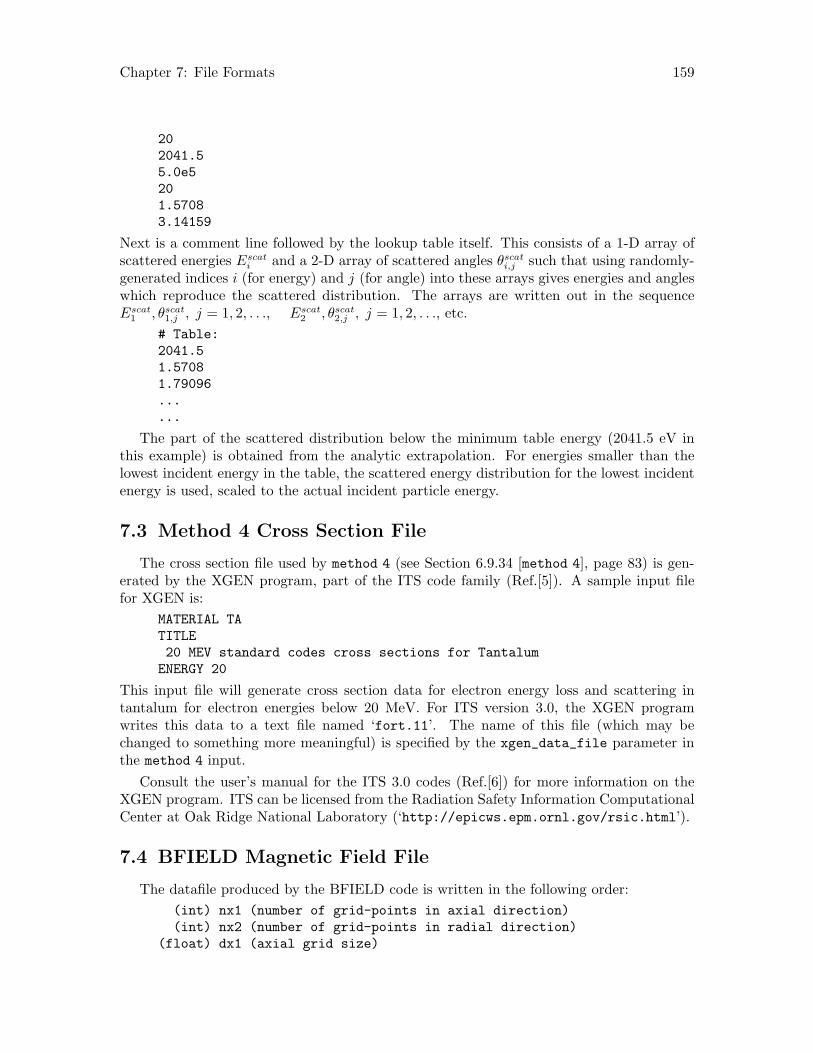
Chapter 7: File Formats 159
202041.55.0e5201.57083.14159
Next is a comment line followed by the lookup table itself. This consists of a 1-D array ofscattered energies Escat
i and a 2-D array of scattered angles θscati,j such that using randomly-
generated indices i (for energy) and j (for angle) into these arrays gives energies and angleswhich reproduce the scattered distribution. The arrays are written out in the sequenceEscat
1 , θscat1,j , j = 1, 2, . . ., Escat
2 , θscat2,j , j = 1, 2, . . ., etc.
# Table:2041.51.57081.79096......
The part of the scattered distribution below the minimum table energy (2041.5 eV inthis example) is obtained from the analytic extrapolation. For energies smaller than thelowest incident energy in the table, the scattered energy distribution for the lowest incidentenergy is used, scaled to the actual incident particle energy.
7.3 Method 4 Cross Section File
The cross section file used by method 4 (see Section 6.9.34 [method 4], page 83) is gen-erated by the XGEN program, part of the ITS code family (Ref.[5]). A sample input filefor XGEN is:
MATERIAL TATITLE20 MEV standard codes cross sections for TantalumENERGY 20
This input file will generate cross section data for electron energy loss and scattering intantalum for electron energies below 20 MeV. For ITS version 3.0, the XGEN programwrites this data to a text file named ‘fort.11’. The name of this file (which may bechanged to something more meaningful) is specified by the xgen_data_file parameter inthe method 4 input.
Consult the user’s manual for the ITS 3.0 codes (Ref.[6]) for more information on theXGEN program. ITS can be licensed from the Radiation Safety Information ComputationalCenter at Oak Ridge National Laboratory (‘http://epicws.epm.ornl.gov/rsic.html’).
7.4 BFIELD Magnetic Field File
The datafile produced by the BFIELD code is written in the following order:(int) nx1 (number of grid-points in axial direction)(int) nx2 (number of grid-points in radial direction)
(float) dx1 (axial grid size)
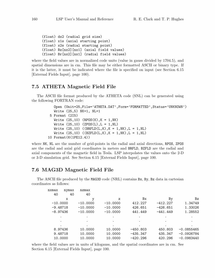
160 LSP User’s Manual and Reference R. E. Clark and T. P. Hughes
(float) dx2 (radial grid size)(float) x1s (axial starting point)(float) x2s (radial starting point)(float) Bz[nx2][nx1] (axial field values)(float) Br[nx2][nx1] (radial field values)
where the field values are in normalized code units (value in gauss divided by 1704.5), andspatial dimensions are in cm. This file may be either formatted ASCII or binary type. Ifit is the latter, it must be indicated where the file is specified on input (see Section 6.15[External Fields Input], page 100).
7.5 ATHETA Magnetic Field File
The ASCII file format produced by the ATHETA code (SNL) can be generated usingthe following FORTRAN code:
Open (Unit=25,File=’ATHETA.DAT’,Form=’FORMATTED’,Status=’UNKNOWN’)Write (25,5) NK+1, NL+1
5 Format (2I5)Write (25,10) (RPOS(K),K = 1,NK)Write (25,10) (ZPOS(L),L = 1,NL)Write (25,10) ((BRFLD(L,K),K = 1,NK),L = 1,NL)Write (25,10) ((BZFLD(L,K),K = 1,NK),L = 1,NL)
10 Format(6(1PE12.4))
where NK, NL are the number of grid-points in the radial and axial directions, RPOS, ZPOSare the radial and axial grid coordinates in meters and BRFLD, BZFLD are the radial andaxial components of the magnetic field in Tesla. LSP interpolates the values onto the 2-Dor 3-D simulation grid. See Section 6.15 [External Fields Input], page 100.
7.6 MAG3D Magnetic Field File
The ASCII file produced by the MAG3D code (NRL) contains Bx, By, Bz data in cartesiancoordinates as follows:
nxmax nymax nzmax40 40 40
x y z Bx By Bz-10.0000 -10.0000 -10.0000 412.227 -412.227 1.34749-9.48718 -10.0000 -10.0000 426.651 -426.651 1.33026-8.97436 -10.0000 -10.0000 441.449 -441.449 1.28552
. . . . . .
. . . . . .
. . . . . .8.97436 10.0000 10.0000 -450.803 450.803 -0.08554659.48718 10.0000 10.0000 -435.347 435.347 -0.092678410.0000 10.0000 10.0000 -420.296 420.296 -0.0983440
where the field values are in units of kilogauss, and the spatial coordinates are in cm. SeeSection 6.15 [External Fields Input], page 100.
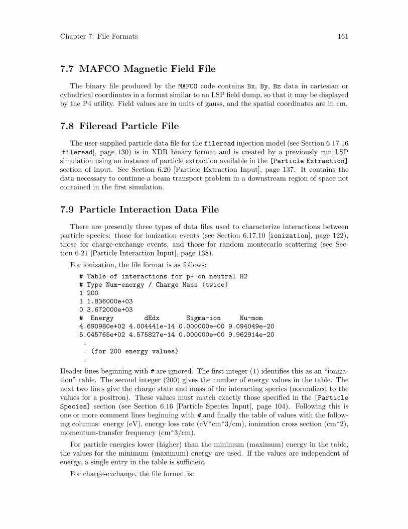
Chapter 7: File Formats 161
7.7 MAFCO Magnetic Field File
The binary file produced by the MAFCO code contains Bx, By, Bz data in cartesian orcylindrical coordinates in a format similar to an LSP field dump, so that it may be displayedby the P4 utility. Field values are in units of gauss, and the spatial coordinates are in cm.
7.8 Fileread Particle File
The user-supplied particle data file for the fileread injection model (see Section 6.17.16[fileread], page 130) is in XDR binary format and is created by a previously run LSPsimulation using an instance of particle extraction available in the [Particle Extraction]section of input. See Section 6.20 [Particle Extraction Input], page 137. It contains thedata necessary to continue a beam transport problem in a downstream region of space notcontained in the first simulation.
7.9 Particle Interaction Data File
There are presently three types of data files used to characterize interactions betweenparticle species: those for ionization events (see Section 6.17.10 [ionization], page 122),those for charge-exchange events, and those for random montecarlo scattering (see Sec-tion 6.21 [Particle Interaction Input], page 138).
For ionization, the file format is as follows:
# Table of interactions for p+ on neutral H2# Type Num-energy / Charge Mass (twice)1 2001 1.836000e+030 3.672000e+03# Energy dEdx Sigma-ion Nu-mom4.690980e+02 4.004441e-14 0.000000e+00 9.094049e-205.045765e+02 4.575827e-14 0.000000e+00 9.962914e-20.. (for 200 energy values).
Header lines beginning with # are ignored. The first integer (1) identifies this as an “ioniza-tion” table. The second integer (200) gives the number of energy values in the table. Thenext two lines give the charge state and mass of the interacting species (normalized to thevalues for a positron). These values must match exactly those specified in the [ParticleSpecies] section (see Section 6.16 [Particle Species Input], page 104). Following this isone or more comment lines beginning with # and finally the table of values with the follow-ing columns: energy (eV), energy loss rate (eV*cm^3/cm), ionization cross section (cm^2),momentum-transfer frequency (cm^3/cm).
For particle energies lower (higher) than the minimum (maximum) energy in the table,the values for the minimum (maximum) energy are used. If the values are independent ofenergy, a single entry in the table is sufficient.
For charge-exchange, the file format is:

162 LSP User’s Manual and Reference R. E. Clark and T. P. Hughes
# Table of interactions for neutral H2 on p+# Type Num-energy / Charge Mass (twice)2 2000 3.672000e+031 1.836000e+03# Energy Nu-cx Nu-mom4.690980e+02 8.536466e-20 5.575825e-215.045765e+02 9.405332e-20 5.575825e-21.. (for 200 energy values).
The first integer (2) identifies this as a “charge-exchange” table. The next two linesare the same as for the ionization table above. The table of values has the followingcolumns: energy (eV), momentum-transfer frequency due to charge-exchange (cm^3/cm),and momentum-transfer frequency due to scattering (cm^3/cm).
For montecarlo scattering, the file format is as follows:# Table of interactions for e- on neutral He (Montecarlo type)# Type Num-energy / Charge Mass (twice)3 460-1 1.000000e+000 7.344000e+03# number of inelastic processes (nproc)7# Eaniso Eioniz Bparam Delta_E_1 ... Delta_E_nproc0.000000E+00 0.246000E+02 0.000000E+00 0.198000E+02 ... 0.240000E+02# Energy Sigma_el Sigma_ioniz Sigma_1 ... Sigma_nproc0.000000E+00 0.495000E-15 0.000000E+00 0.000000E+00 ... 0.000000E+000.100000E+00 0.579524E-15 0.000000E+00 0.000000E+00 ... 0.000000E+00.. (for 460 energy values).
7.10 Primary Output Data File
The primary output data files have the following format for each particle:WEIGHT X Y Z Vx Vy Vz
where WEIGHT is the charge weight of the macro-particle, the X/Y/Z coordinates arein cm, and the V’s are the gamma-beta velocity components. The data can be spreadonto discrete files, depending on the extraction_dump_interval or its related controlparameters. The resulting files will have names like ‘primNNNN.dat’, where ‘NNNN’ is thetimestep on which the data is finalized. If no dump interval or dump time is specified, allof the data will remain on a file named ‘primaries.dat’.
7.11 Photon Output Data File
The photon output data files have the following format for each photon:
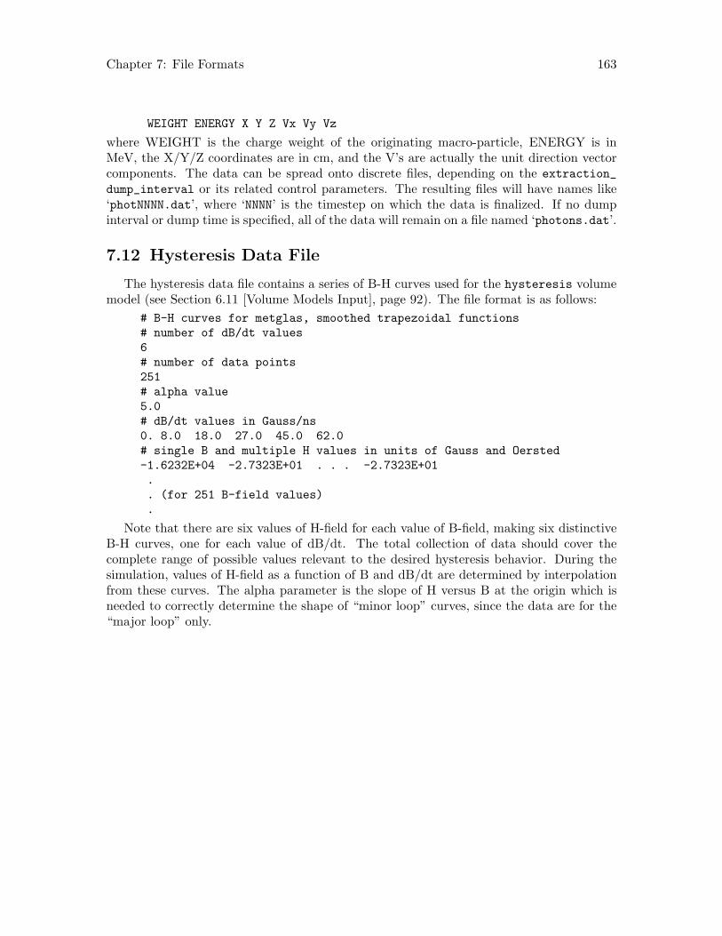
Chapter 7: File Formats 163
WEIGHT ENERGY X Y Z Vx Vy Vz
where WEIGHT is the charge weight of the originating macro-particle, ENERGY is inMeV, the X/Y/Z coordinates are in cm, and the V’s are actually the unit direction vectorcomponents. The data can be spread onto discrete files, depending on the extraction_dump_interval or its related control parameters. The resulting files will have names like‘photNNNN.dat’, where ‘NNNN’ is the timestep on which the data is finalized. If no dumpinterval or dump time is specified, all of the data will remain on a file named ‘photons.dat’.
7.12 Hysteresis Data File
The hysteresis data file contains a series of B-H curves used for the hysteresis volumemodel (see Section 6.11 [Volume Models Input], page 92). The file format is as follows:
# B-H curves for metglas, smoothed trapezoidal functions# number of dB/dt values6# number of data points251# alpha value5.0# dB/dt values in Gauss/ns0. 8.0 18.0 27.0 45.0 62.0# single B and multiple H values in units of Gauss and Oersted-1.6232E+04 -2.7323E+01 . . . -2.7323E+01.. (for 251 B-field values).
Note that there are six values of H-field for each value of B-field, making six distinctiveB-H curves, one for each value of dB/dt. The total collection of data should cover thecomplete range of possible values relevant to the desired hysteresis behavior. During thesimulation, values of H-field as a function of B and dB/dt are determined by interpolationfrom these curves. The alpha parameter is the slope of H versus B at the origin which isneeded to correctly determine the shape of “minor loop” curves, since the data are for the“major loop” only.

164 LSP User’s Manual and Reference R. E. Clark and T. P. Hughes
Chapter 8: Utilities 165
8 Utilities
8.1 Perleval Preprocessor
Perleval is a Perl script which allows one to define and use symbolic names in the LSPinput file. Variable names must begin with a ‘$’ character, and expressions (including singlevariables) are enclosed in curly brackets ‘{}’. Variables may be defined in a comment sectionat the top of the input file, and then expressions using these variables may appear anywherewithin the input file. Essentially the same capability is built into the GLSP preprocessor(see Section 1.2 [GLSP Preprocessor], page 2), which uses the Tcl expression evaluator.There are some syntax differences due to the differences between Perl and Tcl expressions(e.g., the exponentiation operator is ‘**’ in Perl and ‘pow’ in Tcl.)
8.2 Renumber Utility
Various keywords in the LSP input file, such as object and probe, have integers ap-pended to them. The integer provides identification for the associated item, but makes itinconvenient to insert new items, since subsequent items must then be renumbered. The‘renumber’ utility automates renumbering to renumber the probes in the file ‘input.lsp’,type
renumber probe input.lsp
The GLSP preprocessor (see Section 1.2 [GLSP Preprocessor], page 2) does automaticrenumbering.

166 LSP User’s Manual and Reference R. E. Clark and T. P. Hughes
Chapter 9: References 167
9 References
[1] M. Chapman and E. Waisman, J. Comp. Phys. 58, 44, 1985.[2] B. I. Cohen, A. B. Langdon, and A. Friedman, J. Comp. Phys. 46, 15 (1982); A. B.Langdon and D. C. Barnes, “Direct Implicit Plasma Simulation,” Multiple Time Scales,edited by J. U. Brackbill and B. I. Cohen (Academic Press, Orlando, FL, 1985), p. 335.[3] Alex Friedman, “A Second-order Implicit Particle Mover with Adjustable Damping,” J.Comp. Phys. 90, 292 (1990).[4] B. B. Godfrey, Time-biased Field Solver for Electromagnetic PIC Codes, Presented atNinth Conference on Numerical Simulation of Plasmas, AMRC-N-138 (1980).[5] J. A. Halbleib, R. P. Kensek, G. D. Valdez, S. M. Seltzer, and M. J. Berger, “ITS: TheIntegrated TIGER Series of electron/photon transport codes - version 3.0,” IEEE Trans.Nucl. Sci. NS-39, 1025 (1992).[6] J. A. Halbleib, R. P. Kensek, T. A. Melhorn, G. D. Valdez, S. M. Seltzer, and M.J. Berger, “ITS Version 3.0: The Integrated TIGER Series of Coupled Electron/PhotonTransport Codes,” SAND91-1634, Sandia National Laboratories, March 1992.[7] B. L. Henke, E. M. Gullikson, and J. C. Davis, “X-ray interactions: photoabsorption,scattering, transmission, and reflection at E = 50 - 30,000 eV, Z = 1 - 92,” Atomic Dataand Nucl. Data Tables 54, 181 (1993).[8] T. G. Jurgens, A. Taflove, K. Umashankar, and T. G. Moore, “Finite-Difference Time-Domain Modeling of Curved Surfaces,” IEEE Transactions on Antennas and Propagation40, 357 (1992); T. G. Jurgens and A. Taflove, “Three-Dimensional Contour FDTD Model-ing of Scattering from Single and Multiple Bodies,” IEEE Transactions on Antennas andPropagation 41, 1703 (1993).[9] P. Rambo, J. Ambrosiano, A. Friedman, and D. E. Nielsen Jr., Temporal and SpatialFiltering Remedies for Dispersion in Electromagnetic Particle Codes, Proc. 13th Conferenceon the Numerical Simulation of Plasmas, 1989.[10] W. M. Sharp, D. A. Callahan-Miller, A. B. Langdon, M. S. Armel and J.-L. Vay,“Improved modeling of chamber transport for heavy-ion fusion,” Nucl. Meth. Phys. Res.A 464, 284 (2001).[11] A. Taflove, “Computational Electrodynamics,” (Artech House, 1995), p. 228.[12] R. A. Vesey, “Effect of backscattered/secondary electrons on neutral layer ionization,”Technical Memorandum, Aug. 13 1996, Sandia National Laboratories.[13] D. D. Hinshelwood, “BERTHA - A Versatile Transmission Line and Circuit Code,”NRL Memorandum Report 5185, Nov. 21 1983, Naval Research Laboratory.

168 LSP User’s Manual and Reference R. E. Clark and T. P. Hughes
Chapter 10: General Index 169
10 General Index
11-D coordinates, CAR_ONE . . . . . . . . . . . . . . . . . . . . . 151-D coordinates, CYL_ONE . . . . . . . . . . . . . . . . . . . . . 161-D coordinates, Grid . . . . . . . . . . . . . . . . . . . . . . . . 521-D coordinates, SPH_ONE . . . . . . . . . . . . . . . . . . . . . 21
22-D coordinates, CAR_X_Y . . . . . . . . . . . . . . . . . . . . . 152-D coordinates, CAR_X_Z . . . . . . . . . . . . . . . . . . . . . 152-D coordinates, CYL_R_TH . . . . . . . . . . . . . . . . . . . . 162-D coordinates, CYL_R_Z . . . . . . . . . . . . . . . . . . . . . 162-D coordinates, Grid . . . . . . . . . . . . . . . . . . . . . . . . 522-D coordinates, SPH_R_TH . . . . . . . . . . . . . . . . . . . . 212-D functions . . . . . . . . . . . . . . . . . . . . . . . . . . . . . . . 1452-D scattering - sample input . . . . . . . . . . . . . . . . . 812-D scattering, method 2 . . . . . . . . . . . . . . . . . . . . . 81
33-D coordinates, CARTESIAN . . . . . . . . . . . . . . . . . . . 153-D coordinates, CYLINDRICAL . . . . . . . . . . . . . . . . 163-D coordinates, Grid . . . . . . . . . . . . . . . . . . . . . . . . 523-D coordinates, SPHERICAL . . . . . . . . . . . . . . . . . . . 22
44-D backscattering - sample input . . . . . . . . . . . . . 824-D backscattering, method 3 . . . . . . . . . . . . . . . . . 82
Aabort - Command File . . . . . . . . . . . . . . . . . . . . . . . 11acceleration_parameter - definition . . . . . . . . . . 38ADI field solver, dielectric . . . . . . . . . . . . . . . . . . 94ADI field solver, DIRECT_IMPLICIT . . . . . . . . . . . . 16ADI field solver, ferrite . . . . . . . . . . . . . . . . . . . . . 95ADI field solver,
implicit_acceleration_parameter . . . . . . 37ADI field solver, IMPLICIT_FIELDS . . . . . . . . . . . . 19ADI field solver, implicit_iterations . . . . . . . . 37ADI field solver, implicit_omega_min_factor . . 37ADI field solver, implicit_subcycles . . . . . . . . . 37ADI field solver, implicit_tolerance . . . . . . . . . 38ADI field solver, paramagnetic . . . . . . . . . . . . . . . 96ADI field solver, USE_PERMEABILITY . . . . . . . . . . . 23ADI field solver, USE_PERMITTIVITY . . . . . . . . . . . 23air . . . . . . . . . . . . . . . . . . . . . . . . . . . . . . . . . . . . . . 75, 78air chemistry, conductivity (medium) . . . . . . . . 76air chemistry, USE_OHMIC_TERMS . . . . . . . . . . . . . . . 23air chemistry, vcrossb_flag . . . . . . . . . . . . . . . . . . 39air_model - definition . . . . . . . . . . . . . . . . . . . . . . . . 75algorithm, direct-implicit . . . . . . . . . . . . . . . . . . . . 106algorithm, electromagnetic field . . . . . . . . . . . . . . . . 1
algorithm, implicit plasma . . . . . . . . . . . . . . . . . . . . 37algorithm, moving frame . . . . . . . . . . . . . . . . . . . . . 40algorithm, particles . . . . . . . . . . . . . . . . . . . . . . . . . . . 2algorithms, list of . . . . . . . . . . . . . . . . . . . . . . . . . . . . . 2algorithms, LSP Simulation Code . . . . . . . . . . . . . . 1alignment_axis - definition . . . . . . . . . . . . . . . . . 103alignment_axis, symmetry_direction . . . . . . . 103aluminum . . . . . . . . . . . . . . . . . . . . . . . . . . . . . . . . 72, 78applied_current - definition . . . . . . . . . . . . . . . . . 34applied_current, hysteresis . . . . . . . . . . . . . . . . 95argon . . . . . . . . . . . . . . . . . . . . . . . . . . . . . . . . . . . . 75, 78ASCIQ . . . . . . . . . . . . . . . . . . . . . . . . . . . . . . . . . . . . . . . 9ATHETA Magnetic Field File . . . . . . . . . . . . . . . 160atomic_number . . . . . . . . . . . . . . . . . . . . . . . . . . . . . . 72atomic_number - definition . . . . . . . . . . . . . . . . . . 105atomic_weight . . . . . . . . . . . . . . . . . . . . . . . . . . . . . . 72avalanche ionization, conductivity (medium) . . 76azimuthal_angle - definition . . . . . . . . . . . . . . . . . 77
BB . . . . . . . . . . . . . . . . . . . . . . . . . . . . . . . . . . . . . . 148, 150background runs, Single-Processor Machines . . . . 7background_electron_conductivity - definition
. . . . . . . . . . . . . . . . . . . . . . . . . . . . . . . . . . . . . . . . 34background_plasma_density - definition . . . . . . 34backscatter - definition . . . . . . . . . . . . . . . . . . . . 119backscatter - sample input . . . . . . . . . . . . . . . . . 119backscatter, method 3 . . . . . . . . . . . . . . . . . . . . . . . 82backscatter_data_file - definition . . . . . . . . . . . 83balance - Command File . . . . . . . . . . . . . . . . . . . . . 11balance_interval - definition . . . . . . . . . . . . . . . . 32balance_interval, load_balance_flag . . . . . . . 33batch runs . . . . . . . . . . . . . . . . . . . . . . . . . . . . . . . . . . . 9BFIELD Magnetic Field File . . . . . . . . . . . . . . . . 159binding_energy - definition . . . . . . . . . . . . . . . . . 121BLOCK - definition . . . . . . . . . . . . . . . . . . . . . . . . . . . . 57BLOCK - sample input . . . . . . . . . . . . . . . . . . . . . . . . . 57BLOCK, FOIL . . . . . . . . . . . . . . . . . . . . . . . . . . . . . . . . . 58BNODE . . . . . . . . . . . . . . . . . . . . . . . . . . . . . . . . . . . . . . 148boundaries - defined . . . . . . . . . . . . . . . . . . . . . . . . . 63Boundaries Input . . . . . . . . . . . . . . . . . . . . . . . . . . . . 63Boundary Errors . . . . . . . . . . . . . . . . . . . . . . . . . . . . . 11breakdown_function - definition . . . . . . . . . . . . . 113
CC compiler, Compiling on MS Windows . . . . . . . 13capacitance - definition . . . . . . . . . . . . . . . . . . . . . 90CAR_ONE - compiler directives . . . . . . . . . . . . . . . . . 15CAR_X_Y - compiler directives . . . . . . . . . . . . . . . . . 15CAR_X_Z - compiler directives . . . . . . . . . . . . . . . . . 15carbon . . . . . . . . . . . . . . . . . . . . . . . . . . . . . . . . . . 72, 78CARTESIAN - compiler directives . . . . . . . . . . . . . . . 15

170 LSP User’s Manual and Reference R. E. Clark and T. P. Hughes
centroid1&2_function - definition . . . . . . . . . . . 110CGS Units . . . . . . . . . . . . . . . . . . . . . . . . . . . . . . . . . . 25charge - definition . . . . . . . . . . . . . . . . . . . . . . . . . . 105charge-exchange, Particle Interaction Data File
. . . . . . . . . . . . . . . . . . . . . . . . . . . . . . . . . . . . . . . 161charge-exchange, Particle Interaction Input . . . 138CHARGE_DENSITY - compiler directives . . . . . . . . . . 15CHARGE_DENSITY, dump_charge_density_flag . . 40CHARGE_DENSITY, dump_rho_background_flag . . 43CHARGE_DENSITY, scalar_movie_components . . . 46CHARGE_DENSITY, STATIC_FIELDS . . . . . . . . . . . . . . 22CHARGE_DEPOSITION - compiler directives . . . . . . 15CHARGE_DEPOSITION,
dump_surface_depositions_flag . . . . . . . . . 43CHARGE_DEPOSITION, emission (stimulated) . . . 114charge_factor (stimulated) - definition . . . . . . 115charge_factor (stimulated), emission
(stimulated) . . . . . . . . . . . . . . . . . . . . . . . . . . . . 114charge_factor - definition . . . . . . . . . . . . . . . . . . 110charge_weight - definition . . . . . . . . . . . . . . . . . . 133Child-Langmuir emission - sample input . . . . . . 111CIC (cloud-in-cell), EXTENDED_PARTICLES . . . . . . 17CIC (cloud-in-cell), LSP Simulation Code . . . . . . . 2circuit - definition . . . . . . . . . . . . . . . . . . . . . . . . . . 67circuit model - sample input . . . . . . . . . . . . . . . . . . 85Circuit Model Probes . . . . . . . . . . . . . . . . . . . . . . . 155Circuit Models Input . . . . . . . . . . . . . . . . . . . . . . . . . 85Circuit Models Input, circuit . . . . . . . . . . . . . . . . 67Circuit Models Input, connection_rank . . . . . . . 67Circuit Models Input, Outlet Boundaries . . . . . . 63Circuit Models Input, temporal_function (outlet
boundary) . . . . . . . . . . . . . . . . . . . . . . . . . . . . . . 68circuit, voltage_measurement . . . . . . . . . . . . . . . 68cloud-in-cell (CIC), EXTENDED_PARTICLES . . . . . . 17cloud-in-cell (CIC), LSP Simulation Code . . . . . . . 2coax, boundaries - sample input . . . . . . . . . . . . . . . 64cold_test_flag - definition . . . . . . . . . . . . . . . . . . 34collision frequencies, Particle Interaction Data File
. . . . . . . . . . . . . . . . . . . . . . . . . . . . . . . . . . . . . . . 161collision_energies - definition . . . . . . . . . . . . . . 78collision_energies, scatter_angles . . . . . . . . 81collisional plasma model,
dump_montecarlo_diagnostics_flag . . . . . 41collisional plasma model, fluid_species_flag
. . . . . . . . . . . . . . . . . . . . . . . . . . . . . . . . . . . . . . . 106collisional plasma model, IONIZATION_ON . . . . . . 19collisional plasma model, migrant_species_flag
. . . . . . . . . . . . . . . . . . . . . . . . . . . . . . . . . . . . . . . 106collisional plasma model,
montecarlo_scattering_flag . . . . . . . . . . . 107collisional plasma model, SCATTERING_ON . . . . . . 21COLLISIONAL_PLASMA - compiler directives . . . . . 16COLLISIONAL_PLASMA, FLUID_PHYSICS . . . . . . . . . 18COLLISIONAL_PLASMA, FRICTIONAL_EFFECTS . . . . 18COLLISIONAL_PLASMA, IONIZATION_ON . . . . . . . . . 19COLLISIONAL_PLASMA, Particle Interaction Input
. . . . . . . . . . . . . . . . . . . . . . . . . . . . . . . . . . . . . . . 138COLLISIONAL_PLASMA, SCATTERING_ON . . . . . . . . . 21
collisions, conductivity (medium) . . . . . . . . . . . . 76collisions, LSP Simulation Code . . . . . . . . . . . . . . . . 2collisions, Particle Interaction Data File . . . . . . 161collisions, Particle Interaction Input . . . . . . . . . . 138Command File . . . . . . . . . . . . . . . . . . . . . . . . . . . . . . 11Command File, Running LSP . . . . . . . . . . . . . . . . . . 7comments . . . . . . . . . . . . . . . . . . . . . . . . . . . . . . . . . . . 28compilation errors . . . . . . . . . . . . . . . . . . . . . . . . . . . 14Compiler Directives . . . . . . . . . . . . . . . . . . . . . . . . . . 15compiler directives, Compiling on MS Windows
. . . . . . . . . . . . . . . . . . . . . . . . . . . . . . . . . . . . . . . . 14compiler directives, Grid . . . . . . . . . . . . . . . . . . . . . 52compiler directives, Regions Input . . . . . . . . . . . . . 55compiler directives, Startup Messages . . . . . . . . . 10compiler directives, User Units . . . . . . . . . . . . . . . . 25Compiling LSP . . . . . . . . . . . . . . . . . . . . . . . . . . . . . . 13compiling LSP, Startup Messages . . . . . . . . . . . . . 10complex magnetic permeability model,
MAGNETIC_DISPERSION . . . . . . . . . . . . . . . . . . . 20components - definition . . . . . . . . . . . . . . . . . . . . . . . 78components, conductivity (medium) . . . . . . . . . 76components, list of . . . . . . . . . . . . . . . . . . . . . . . . . . . 78Computational Solid Geometry (CSG) . . . . . . . . 56conductivity (medium) - definition . . . . . . . . . . . 76conductivity - definition . . . . . . . . . . . . . . . . . . . . 93conductivity, dump_ohmic_quantities_flag . . 42conductivity, method 1 - sample input . . . . . . . . . 80conductors, Objects Input . . . . . . . . . . . . . . . . . . . . 56CONE - definition . . . . . . . . . . . . . . . . . . . . . . . . . . . . . 58CONE - sample input . . . . . . . . . . . . . . . . . . . . . . . . . . 58connection_rank - definition . . . . . . . . . . . . . . . . . 67control - sample input . . . . . . . . . . . . . . . . . . . . . . . . 30Control Input . . . . . . . . . . . . . . . . . . . . . . . . . . . . . . . 30Control Input, extract_photons_flag . . . . . . . . 77Control Input, extract_primaries_flag . . . . . . 77Control Input, extract_secondaries_flag . . . . 77Control Input, ionization . . . . . . . . . . . . . . . . . . 122Control Input, Particle Targets Input . . . . . . . . 143Conventions . . . . . . . . . . . . . . . . . . . . . . . . . . . . . . . . . . 5conventions - coordinates . . . . . . . . . . . . . . . . . . . . . . 5conventions - document . . . . . . . . . . . . . . . . . . . . . . . 5conventions - fonts . . . . . . . . . . . . . . . . . . . . . . . . . . . . 5conventions - index . . . . . . . . . . . . . . . . . . . . . . . . . . . 5convergence - definition . . . . . . . . . . . . . . . . . . . . 118Convergence Probes - definition . . . . . . . . . . . . . . 154Convergence Probes, implicit_iterations . . . . 37Convergence Probes, potential_iterations . . . 38convergence_iterations - definition . . . . . . . . . . 34convergence_tolerance - definition . . . . . . . . . . . 34conversion_rate - definition . . . . . . . . . . . . . . . . 129convolutional PML model - sample input . . . . . . 69Coordinate-system dependent shape, BLOCK . . . . 57Coordinate-system dependent shape, FOIL . . . . . 59Coordinate-system dependent shape, FUNCTION
. . . . . . . . . . . . . . . . . . . . . . . . . . . . . . . . . . . . . . . . 59Coordinate-system dependent shape,
QUADRILATERAL . . . . . . . . . . . . . . . . . . . . . . . . . . 60

Chapter 10: General Index 171
Coordinate-system dependent shape, TRILATERAL. . . . . . . . . . . . . . . . . . . . . . . . . . . . . . . . . . . . . . . . 60
Coordinate-system dependent shape, WIRE . . . . . 62Coordinate-system independent shape, CONE . . . 58Coordinate-system independent shape, CYLINDER
. . . . . . . . . . . . . . . . . . . . . . . . . . . . . . . . . . . . . . . . 58Coordinate-system independent shape, PARABOLOID
. . . . . . . . . . . . . . . . . . . . . . . . . . . . . . . . . . . . . . . . 59Coordinate-system independent shape,
PARALLELEPIPED . . . . . . . . . . . . . . . . . . . . . . . . . 60Coordinate-system independent shape, SPHERE
. . . . . . . . . . . . . . . . . . . . . . . . . . . . . . . . . . . . . . . . 61Coordinate-system independent shape, TORUS . . 61coordinates, CAR_ONE . . . . . . . . . . . . . . . . . . . . . . . . . 15coordinates, CAR_X_Y . . . . . . . . . . . . . . . . . . . . . . . . . 15coordinates, CAR_X_Z . . . . . . . . . . . . . . . . . . . . . . . . . 15coordinates, CARTESIAN . . . . . . . . . . . . . . . . . . . . . . . 15coordinates, Conventions . . . . . . . . . . . . . . . . . . . . . . 5coordinates, courant_multiplier . . . . . . . . . . . . . 30coordinates, CYL_ONE . . . . . . . . . . . . . . . . . . . . . . . . . 16coordinates, CYL_R_TH . . . . . . . . . . . . . . . . . . . . . . . . 16coordinates, CYL_R_Z . . . . . . . . . . . . . . . . . . . . . . . . . 16coordinates, CYLINDRICAL . . . . . . . . . . . . . . . . . . . . 16coordinates, Grid . . . . . . . . . . . . . . . . . . . . . . . . . . . . 52coordinates, LSP Simulation Code . . . . . . . . . . . . . 1coordinates, print_grid_flag . . . . . . . . . . . . . . . . 50coordinates, Regions Input . . . . . . . . . . . . . . . . . . . 54coordinates, small_radius_exlusion . . . . . . . . . . 36coordinates, SPH_ONE . . . . . . . . . . . . . . . . . . . . . . . . . 21coordinates, SPH_R_TH . . . . . . . . . . . . . . . . . . . . . . . . 21coordinates, SPHERICAL . . . . . . . . . . . . . . . . . . . . . . . 22coordinates, VOLUME_WEIGHTING . . . . . . . . . . . . . . . 24copper . . . . . . . . . . . . . . . . . . . . . . . . . . . . . . . . . . . 72, 78Coulomb collisions, Particle Interaction Input
. . . . . . . . . . . . . . . . . . . . . . . . . . . . . . . . . . . . . . . 138courant_multiplier - definition . . . . . . . . . . . . . . 30CPU time, dump_timing_flag . . . . . . . . . . . . . . . . 50CPU time, Performance Probes . . . . . . . . . . . . . . 155CPU time, report_timing_flag . . . . . . . . . . . . . . 51cross sections, higherstate . . . . . . . . . . . . . . . . . . 124cross sections, ionization . . . . . . . . . . . . . . . . . . . 122cross sections, Method 4 Cross Section File . . . 159cross sections, Particle Interaction Data File . . 161cross sections, Particle Interaction Input . . . . . . 138cross sections, poloidal_angles . . . . . . . . . . . . . . 81cross sections, spatial_function (injection) . . 116cross sections, stimulated_cross_section . . . . 121cross_section_file - definition . . . . . . . . . . . . . 126cross_sections (fragmentation) - definition . . 130cross_sections (higherstate) - definition . . . . . 124CSG (Computational Solid Geometry) . . . . . . . . 56CURRENT_CORRECTION - compiler directives . . . . . 16CURRENTS_OFF - compiler directives . . . . . . . . . . . . 16cyclotron frequency, particle_cyclotron_check
. . . . . . . . . . . . . . . . . . . . . . . . . . . . . . . . . . . . . . . . 50cyclotron frequency, SUBCYCLING_ON . . . . . . . . . . . 22CYL_ONE - compiler directives . . . . . . . . . . . . . . . . . 16CYL_R_TH - compiler directives . . . . . . . . . . . . . . . . 16
CYL_R_Z - compiler directives . . . . . . . . . . . . . . . . . 16CYL_R_Z, dump_rbtheta_current_flag . . . . . . . . 42CYL_R_Z, scalar_movie_components . . . . . . . . . . 46CYLINDER - definition . . . . . . . . . . . . . . . . . . . . . . . . . 58CYLINDER - sample input . . . . . . . . . . . . . . . . . . . . . 58CYLINDRICAL - compiler directives . . . . . . . . . . . . . 16CYLINDRICAL, courant_multiplier . . . . . . . . . . . . 30CYLINDRICAL, dump_rbtheta_current_flag . . . . 42CYLINDRICAL, scalar_movie_components . . . . . . 46
Ddata formats, Data Type Errors . . . . . . . . . . . . . . . 14data formats, LSP Simulation Code . . . . . . . . . . . . 2Data Type Errors . . . . . . . . . . . . . . . . . . . . . . . . . . . . 14Debye relaxation, ferrite . . . . . . . . . . . . . . . . . . . . 94Debye, LSP Simulation Code . . . . . . . . . . . . . . . . . . 2DEC Cluster . . . . . . . . . . . . . . . . . . . . . . . . . . . . . . . . . 8decomposition, LSP Simulation Code . . . . . . . . . . . 1DEDT . . . . . . . . . . . . . . . . . . . . . . . . . . . . . . . . . . . . . . . 150deflection1&2_angle - definition . . . . . . . . . . . . 117deflection1&2_function - definition . . . . . . . . . 117DELAY_BREAKDOWN - compiler directives . . . . . . . . . 16DELAY_BREAKDOWN, breakdown_function . . . . . . 113DENSE medium, thickness . . . . . . . . . . . . . . . . . . . . 80DENSE, ENERGY_DEPOSITION . . . . . . . . . . . . . . . . . . . 17density - definition . . . . . . . . . . . . . . . . . . . . . . . . . . 74density_flags (plasma) - definition . . . . . . . . . 128density_flags, density_function (plasma) . . 127density_function (plasma) - definition . . . . . . 127desorption - definition. . . . . . . . . . . . . . . . . . . . . . 119desorption - sample input . . . . . . . . . . . . . . . . . . 120DESORPTION_ON - compiler directives . . . . . . . . . . . 16DESORPTION_ON, desorption . . . . . . . . . . . . . . . . . 119Diagnostic Output . . . . . . . . . . . . . . . . . . . . . . . . . . . 40diagnostic_dump_interval - definition . . . . . . . 41diagnostic_dump_interval,
dump_substrates_flag . . . . . . . . . . . . . . . . . . 43diagnostic_dump_interval, Particle Diagnostics
Input . . . . . . . . . . . . . . . . . . . . . . . . . . . . . . . . . . 140diagnostic_dump_interval, Particle Targets
Input . . . . . . . . . . . . . . . . . . . . . . . . . . . . . . . . . . 142diagnostic_dump_steps - definition . . . . . . . . . . . 43diagnostic_dump_times - definition . . . . . . . . . . . 44diagnostics, CHARGE_DENSITY . . . . . . . . . . . . . . . . . . 15diagnostics, dump_interval . . . . . . . . . . . . . . . . . . . 41diagnostics, dump_steps . . . . . . . . . . . . . . . . . . . . . . 43diagnostics, dump_substrates_flag . . . . . . . . . . . 43diagnostics, dump_times . . . . . . . . . . . . . . . . . . . . . . 44diagnostics, method 4 . . . . . . . . . . . . . . . . . . . . . . . . 83diagnostics, NUMBER_DENSITIES . . . . . . . . . . . . . . . 21diagnostics, Particle Diagnostics Input . . . . . . . 140diagnostics, Particle Targets Input . . . . . . . . . . . 142diagnostics, Probes Input . . . . . . . . . . . . . . . . . . . . 148diagnostics, slice_times . . . . . . . . . . . . . . . . . . . . 111dielectric - definition . . . . . . . . . . . . . . . . . . . . . . . 93dielectric material - sample input . . . . . . . . . . . . . 79dielectric materials . . . . . . . . . . . . . . . . 34, 73, 79, 93
172 LSP User’s Manual and Reference R. E. Clark and T. P. Hughes
dielectric materials, dielectric_constant . . . . . 73dielectric materials, USE_PERMITTIVITY . . . . . . . . 23dielectric_constant - definition . . . . . . . . . . . . . 73dielectric_constant, method 0 . . . . . . . . . . . . . . 79dielectric_constant, segments . . . . . . . . . . . . . . 87dielectric_kill_flag - definition . . . . . . . . . . . . 34diffusion_length - definition . . . . . . . . . . . . . . . . 75dipole - definition . . . . . . . . . . . . . . . . . . . . . . . . . . . 94dipole - sample input . . . . . . . . . . . . . . . . . . . . . . . . 94DIRECT_IMPLICIT - compiler directives . . . . . . . . . 16DIRECT_IMPLICIT,
electric_force_filtering_paramter . . . . 35DIRECT_IMPLICIT, FRICTIONAL_EFFECTS . . . . . . . 18DIRECT_IMPLICIT, FULL_SUSCEPTIBILITY . . . . . . 19DIRECT_IMPLICIT, IMPLICIT_FIELDS . . . . . . . . . . 19DIRECT_IMPLICIT, implicit_iterations . . . . . . 37DIRECT_IMPLICIT, implicit_species_flag . . . 106DIRECT_IMPLICIT, implicit_subcycles . . . . . . . 37DIRECT_IMPLICIT,
magnetic_force_filtering_parameter . . . 35DIRECT_IMPLICIT, Particle Species Input . . . . . 105Dirichlet boundary conditions . . . . . . . . . . . . . . . . . 71discrete_numbers - definition . . . . . . . . . . . . . . . 109documentation . . . . . . . . . . . . . . . . . . . . . . . . . . . . . . 13domain_boundary_check - definition . . . . . . . . . . . 49domain_boundary_check, Boundaries Input . . . . 63domains, dump_timing_flag . . . . . . . . . . . . . . . . . . 50domains, LSP Simulation Code . . . . . . . . . . . . . . . . 1domains, MULTI_PROCESS . . . . . . . . . . . . . . . . . . . . . 20domains, number_of_processes . . . . . . . . . . . . . . . 33domains, Regions Input . . . . . . . . . . . . . . . . . . . . . . 54domains, report_timing_flag . . . . . . . . . . . . . . . . 51DOUBLE_PRECISION - compiler directives . . . . . . . 17drift_momentum - definition . . . . . . . . . . . . . . . . . 110drift_velocity - definition . . . . . . . . . . . . . . . . . 110drive_model - definition . . . . . . . . . . . . . . . . . . . . . 66drive_model, frequency (outlet boundary) . . . . 68drive_model, inner_radius . . . . . . . . . . . . . . . . . . 67drive_model, outer_radius . . . . . . . . . . . . . . . . . . 67drive_model, Outlet Boundaries . . . . . . . . . . . . . . 68drive_model, time_delay . . . . . . . . . . . . . . . . . . . . 68drive_model, voltage_measurement . . . . . . . . . . 68dump - Command File . . . . . . . . . . . . . . . . . . . . . . . . 11dump_accelerations_flag - definition . . . . . . . . . 40dump_bfield_flag - definition . . . . . . . . . . . . . . . . 40dump_charge_density_flag - definition . . . . . . . 40dump_conductivity_flag - definition . . . . . . . . . . 41dump_current_density_flag - definition . . . . . . 41dump_energy_deposition_flag - definition . . . . 41dump_interval - definition . . . . . . . . . . . . . . . . . . . 41dump_montecarlo_diagnostics_flag - definition
. . . . . . . . . . . . . . . . . . . . . . . . . . . . . . . . . . . . . . . . 41dump_number_densities_flag - definition . . . . . 42dump_ohmic_quantities_flag - definition . . . . . 42dump_plasma_quantities_flag - definition . . . . 42dump_potential_flag - definition . . . . . . . . . . . . . 42dump_rbtheta_current_flag - definition . . . . . . 42dump_restart_flag - definition . . . . . . . . . . . . . . . 31
dump_rho_background_flag - definition . . . . . . . 43dump_steps - definition . . . . . . . . . . . . . . . . . . . . . . . 43dump_steps - sample input . . . . . . . . . . . . . . . . . . . 43dump_substrates_flag - definition . . . . . . . . . . . . 43dump_surface_depositions_flag - definition . . 43dump_times - definition . . . . . . . . . . . . . . . . . . . . . . . 44dump_times - sample input . . . . . . . . . . . . . . . . . . . 44dump_timing_flag - definition . . . . . . . . . . . . . . . . 50dump_velocities_flag - definition . . . . . . . . . . . . 44DWDT . . . . . . . . . . . . . . . . . . . . . . . . . . . . . . . . . . . . . . . 150dynamic field solution, Volume Models Input . . 92DYNAMIC_FIELDS - compiler directives . . . . . . . . . . 17DYNAMIC_FIELDS, field_initializatino_flag
. . . . . . . . . . . . . . . . . . . . . . . . . . . . . . . . . . . . . . . . 35
EE . . . . . . . . . . . . . . . . . . . . . . . . . . . . . . . . . . . . . . 148, 150E/p model . . . . . . . . . . . . . . . . . . . . . . . . . . . . . . . . . . 77EDENS . . . . . . . . . . . . . . . . . . . . . . . . . . . . . . . . . . . . . . 148EDEP . . . . . . . . . . . . . . . . . . . . . . . . . . . . . . . . . . 148, 150efficiency . . . . . . . . . . . . . . . . . . . . . . . . . . . . . . . . . . . . . 1electric fields, external, External Fields Input
. . . . . . . . . . . . . . . . . . . . . . . . . . . . . . . . . . . . . . . 100electric fields, external, EXTERNAL_EFIELDS . . . . . 18electric fields, external, field . . . . . . . . . . . . . . . . 102electric_force_filtering_parameter - definition
. . . . . . . . . . . . . . . . . . . . . . . . . . . . . . . . . . . . . . . . 35electric_spatial_filtering_parameter . . . . . 21electric_spatial_filtering_parameter -
definition . . . . . . . . . . . . . . . . . . . . . . . . . . . . . . . 35electron_data_file - definition . . . . . . . . . . . . . . 82electron_density - definition . . . . . . . . . . . . . . . . 77electron_probability - definition . . . . . . . . . . . . 82electron_species (desorption) - definition . . . 121electron_species - definition . . . . . . . . . . . . . . . 109electron_species, photoionization . . . . . . . . 124electrostatic field solver, acceleration_parameter
. . . . . . . . . . . . . . . . . . . . . . . . . . . . . . . . . . . . . . . . 38electrostatic field solver, CHARGE_DENSITY . . . . . . 15electrostatic field solver, Circuit Models Input . . 85electrostatic field solver, Convergence Probes . . 154electrostatic field solver, Objects Input . . . . . . . . 56electrostatic field solver, plasma . . . . . . . . . . . . . . 127electrostatic field solver, potential_iterations
. . . . . . . . . . . . . . . . . . . . . . . . . . . . . . . . . . . . . . . . 38electrostatic field solver, potential_tolerance
. . . . . . . . . . . . . . . . . . . . . . . . . . . . . . . . . . . . . . . . 38electrostatic field solver, Potentials Input . . . . . . 71electrostatic field solver, STATIC_FIELDS . . . . . . . 22electrostatic field solver, STATIC_FIELDS_FFT2D
. . . . . . . . . . . . . . . . . . . . . . . . . . . . . . . . . . . . . . . . 22elements - definition . . . . . . . . . . . . . . . . . . . . . . . . . 87emission (child-langmuir) - definition . . . . . . . . 111emission (field-limited) - definition . . . . . . . . . . 113emission (field-limited) - sample input . . . . . . . 113emission (source-limited) - definition . . . . . . . . 114emission (source-limited) - sample input . . . . . 114

Chapter 10: General Index 173
emission (stimulated) - definition . . . . . . . . . . . . 114emission (stimulated) - sample input . . . . . . . . 114emission (stimulated), STIMULUS_DEPOSITION . . 22emission (stimulated), STIMULUS_SPECIES . . . . . 22emission, discrete_numbers . . . . . . . . . . . . . . . . 109emittance, Particle Measurement Probes . . . . . 150ENERGY_DEPOSITION - compiler directives . . . . . . 17ENERGY_DEPOSITION,
dump_surface_depositions_flag . . . . . . . . . 43ENERGY_DEPOSITION, method 4 . . . . . . . . . . . . . . . . 83ENERGY_DEPOSITION, scalar_movie_components
. . . . . . . . . . . . . . . . . . . . . . . . . . . . . . . . . . . . . . . . 46energy_loss - definition . . . . . . . . . . . . . . . . . . . . . 81energy_loss, KELVIN_DEPOSITION . . . . . . . . . . . . . 19ENODE . . . . . . . . . . . . . . . . . . . . . . . . . . . . . . . . . . . . . . 148episodes - definition . . . . . . . . . . . . . . . . . . . . . . . . 133Error Messages . . . . . . . . . . . . . . . . . . . . . . . . . . . . . . 10error_current_filtering_parameter - definition
. . . . . . . . . . . . . . . . . . . . . . . . . . . . . . . . . . . . . . . . 37errors, boundary . . . . . . . . . . . . . . . . . . . . . . . . . . . . . 11errors, compilation . . . . . . . . . . . . . . . . . . . . . . . . . . . 14errors, data type . . . . . . . . . . . . . . . . . . . . . . . . . . . . . 14errors, incompatible compiler directives . . . . . . . . 15errors, input . . . . . . . . . . . . . . . . . . . . . . . . . . . . . . . . . 11errors, non-halting . . . . . . . . . . . . . . . . . . . . . . . . . . . 10errors, unknown compiler directives . . . . . . . . . . . 14EXACT_IMPLICIT - compiler directives . . . . . . . . . . 17EXACT_IMPLICIT, FULL_SUSCEPTIBILITY . . . . . . . 19excitation - definition. . . . . . . . . . . . . . . . . . . . . . 129excitation - sample input . . . . . . . . . . . . . . . . . . 129EXTENDED_PARTICLES - compiler directives . . . . . 17EXTENDED_PARTICLES, LSP Simulation Code . . . . 2external fields - sample input . . . . . . . . . . . . . . . . 100External Fields Input . . . . . . . . . . . . . . . . . . . . . . . 100External Fields Input, ATHETA Magnetic Field
File . . . . . . . . . . . . . . . . . . . . . . . . . . . . . . . . . . . 160External Fields Input, BFIELD Magnetic Field
File . . . . . . . . . . . . . . . . . . . . . . . . . . . . . . . . . . . 159External Fields Input, EXTERNAL_BFIELDS . . . . . . 17External Fields Input, EXTERNAL_EFIELDS . . . . . . 18External Fields Input, MAFCO Magnetic Field
File . . . . . . . . . . . . . . . . . . . . . . . . . . . . . . . . . . . 161External Fields Input, MAG3D Magnetic Field
File . . . . . . . . . . . . . . . . . . . . . . . . . . . . . . . . . . . 160EXTERNAL_BFIELDS - compiler directives . . . . . . . 17EXTERNAL_BFIELDS, type (external field) . . . . . . 102EXTERNAL_EFIELDS - compiler directives . . . . . . . 18EXTERNAL_EFIELDS, type (external field) . . . . . . 102EXTRA_MOTION - compiler directives . . . . . . . . . . . . 18extract_photons_flag (medium) - definition . . 77extract_photons_flag - definition . . . . . . . . . . . . 44extract_photons_flag, Photon Output Data File
. . . . . . . . . . . . . . . . . . . . . . . . . . . . . . . . . . . . . . . 162extract_primaries_flag (medium) - definition
. . . . . . . . . . . . . . . . . . . . . . . . . . . . . . . . . . . . . . . . 77extract_primaries_flag - definition . . . . . . . . . . 44extract_primaries_flag, Primary Output Data
File . . . . . . . . . . . . . . . . . . . . . . . . . . . . . . . . . . . 162
extract_secondaries_flag (medium) - definition. . . . . . . . . . . . . . . . . . . . . . . . . . . . . . . . . . . . . . . . 77
extract_secondaries_flag - definition . . . . . . . 45extraction_dump_interval - definition . . . . . . . 41extraction_dump_interval,
extract_photons_flag . . . . . . . . . . . . . . . . . . 44extraction_dump_interval,
extract_primaries_flag . . . . . . . . . . . . . . . . 44extraction_dump_interval, Photon Output Data
File . . . . . . . . . . . . . . . . . . . . . . . . . . . . . . . . . . . 162extraction_dump_interval, Primary Output Data
File . . . . . . . . . . . . . . . . . . . . . . . . . . . . . . . . . . . 162extraction_dump_steps - definition . . . . . . . . . . . 43extraction_dump_times - definition . . . . . . . . . . . 44
Fferrite - definition . . . . . . . . . . . . . . . . . . . . . . . . . . 94ferrite, MAGNETIC_DISPERSION . . . . . . . . . . . . . . . 20ferrite, MAX_RESONANCES . . . . . . . . . . . . . . . . . . . . 20field - definition . . . . . . . . . . . . . . . . . . . . . . . . . . . 102Field Solution and Modification . . . . . . . . . . . . . . . 33field solvers . . . . . . . . . . . . . . . . . . . . . . . . . . . . . . . . . 17field_advance_flag - definition . . . . . . . . . . . . . . 35field_dump_interval - definition . . . . . . . . . . . . . 41field_dump_steps - definition . . . . . . . . . . . . . . . . 43field_dump_times - definition . . . . . . . . . . . . . . . . 44field_initialization_flag . . . . . . . . . . . . . . . . . 17field_initialization_flag - definition . . . . . . 35field_movie_components - definition . . . . . . . . . . 45field_movie_components - sample input . . . . . . 45field_movie_coordinate - definition . . . . . . . . . . 45field_movie_coordinate - sample input . . . . . . 45field_movie_interval - definition . . . . . . . . . . . . 45File Formats . . . . . . . . . . . . . . . . . . . . . . . . . . . . . . . 157File Formats, field . . . . . . . . . . . . . . . . . . . . . . . . . 102fileread - definition . . . . . . . . . . . . . . . . . . . . . . . . 130fileread - sample input . . . . . . . . . . . . . . . . . . . . 131Fileread Particle File . . . . . . . . . . . . . . . . . . . . . . . . 161Fileread Particle File, particle_data_file . . . 131fileread, Fileread Particle File . . . . . . . . . . . . . . 161fileread, Particle-Slice Probes . . . . . . . . . . . . . . 153fileread, slice_times . . . . . . . . . . . . . . . . . . . . . 111first_product_species - definition . . . . . . . . . . 130fission - definition . . . . . . . . . . . . . . . . . . . . . . . . . 131fission - sample input . . . . . . . . . . . . . . . . . . . . . 132flag (parameter type) . . . . . . . . . . . . . . . . . . . . . . . . . 5fluid electrons, fluid_species_flag . . . . . . . . . 106fluid electrons, migrant_species_flag . . . . . . . 106Fluid Physics Algorithm . . . . . . . . . . . . . . . . . . . . . . 38fluid_migration_interval - definition . . . . . . . 39FLUID_PHYSICS - compiler directives . . . . . . . . . . . 18FLUID_PHYSICS, electron_species. . . . . . . . . . . 109FLUID_PHYSICS, fluid_migration_interval . . . 39FLUID_PHYSICS, FLUID_SPECIES . . . . . . . . . . . . . . . 18FLUID_PHYSICS, fluid_species_flag . . . . . . . . 106FLUID_PHYSICS, fluid_streaming_factor . . . . . 39FLUID_PHYSICS, flux_limit_fraction . . . . . . . . 39

174 LSP User’s Manual and Reference R. E. Clark and T. P. Hughes
FLUID_PHYSICS, kinetic_migration_interval. . . . . . . . . . . . . . . . . . . . . . . . . . . . . . . . . . . . . . . . 39
FLUID_PHYSICS, Particle Migration Input . . . . . 135FLUID_PHYSICS, pdv_term_flag . . . . . . . . . . . . . . . 39FLUID_PHYSICS, scattering_interval . . . . . . . . 38FLUID_SPECIES - compiler directives . . . . . . . . . . . 18fluid_species_flag - definition . . . . . . . . . . . . . 106fluid_species_flag, FLUID_PHYSICS . . . . . . . . . 18fluid_species_flag, fluid_streaming_factor
. . . . . . . . . . . . . . . . . . . . . . . . . . . . . . . . . . . . . . . . 39fluid_species_flag, flux_limit_fraction . . . 39fluid_species_flag, hybrid_fluid_species
. . . . . . . . . . . . . . . . . . . . . . . . . . . . . . . . . . . . . . . 135fluid_species_flag, hybrid_kinetic_species
. . . . . . . . . . . . . . . . . . . . . . . . . . . . . . . . . . . . . . . 135fluid_species_flag, Particle Extraction Input
. . . . . . . . . . . . . . . . . . . . . . . . . . . . . . . . . . . . . . . 137fluid_species_flag, Particle Migration Input
. . . . . . . . . . . . . . . . . . . . . . . . . . . . . . . . . . . . . . . 135fluid_streaming_factor - definition . . . . . . . . . . 39fluorine . . . . . . . . . . . . . . . . . . . . . . . . . . . . . . . . . . 75, 78flux_limit_fraction - definition . . . . . . . . . . . . . 39focal_length - definition . . . . . . . . . . . . . . . . . . . 118FOIL - definition . . . . . . . . . . . . . . . . . . . . . . . . . . . . . 58FOIL - sample input . . . . . . . . . . . . . . . . . . . . . . . . . . 59foil model, electron_probability . . . . . . . . . . . . 82foil model, primary_probability . . . . . . . . . . . . . 82foil model, secondary . . . . . . . . . . . . . . . . . . . . . . . 118foil model, thickness . . . . . . . . . . . . . . . . . . . . . . . . 80fonts, Conventions . . . . . . . . . . . . . . . . . . . . . . . . . . . . 5format - definition . . . . . . . . . . . . . . . . . . . . . . . . . . 102fragmentation - definition . . . . . . . . . . . . . . . . . . 130fragmentation - sample input . . . . . . . . . . . . . . . 130Freespace Boundaries . . . . . . . . . . . . . . . . . . . . . . . . 69freespace boundaries - sample input . . . . . . . . . . . 69Freespace Boundaries, FREESPACE_PML . . . . . . . . . 18FREESPACE_PML - compiler directives . . . . . . . . . . . 18frequency (outlet boundary) - definition . . . . . . 68frequency - definition . . . . . . . . . . . . . . . . . . . . . . . . 91FRICTIONAL_EFFECTS - compiler directives . . . . . 18from to (backscatter) - definition . . . . . . . . . . . . 119from to (desorption) - definition . . . . . . . . . . . . . 120from to (emission) - definition . . . . . . . . . . . . . . . 112from to (excitation) - definition . . . . . . . . . . . . . . 129from to (external field) - definition . . . . . . . . . . . 102from to (fileread) - definition . . . . . . . . . . . . . . . . 131from to (fission) - definition . . . . . . . . . . . . . . . . . 132from to (fragmentation) - definition . . . . . . . . . . 130from to (higherstate) - definition . . . . . . . . . . . . . 124from to (injection) - definition . . . . . . . . . . . . . . . 116from to (ionization) - definition . . . . . . . . . . . . . . 122from to (outlet boundary) - definition . . . . . . . . . 65from to (particle creation) - definition . . . . . . . . 109from to (photoionization) - definition . . . . . . . . 126from to (plasma) - definition . . . . . . . . . . . . . . . . 127from to (secondary) - definition . . . . . . . . . . . . . . 119from to (stimulated) - definition . . . . . . . . . . . . . 115FULL_SUSCEPTIBILITY - compiler directives . . . . 19
FUNCTION - definition . . . . . . . . . . . . . . . . . . . . . . . . . 59FUNCTION - sample input . . . . . . . . . . . . . . . . . . . . . 59Functions Input . . . . . . . . . . . . . . . . . . . . . . . . . 90, 144Functions Input - sample input . . . . . . . . . . . . . . 144Functions Input, centroid1&2_function . . . . . 110Functions Input, conductivity . . . . . . . . . . . . . . . 93Functions Input, deflection1&2_function . . . 117Functions Input, dielectric . . . . . . . . . . . . . . . . . 93Functions Input, dipole . . . . . . . . . . . . . . . . . . . . . . 94Functions Input, drive_model . . . . . . . . . . . . . . . . 66Functions Input, impedance_product_function
. . . . . . . . . . . . . . . . . . . . . . . . . . . . . . . . . . . . . . . . 91Functions Input, Outlet Bounaries . . . . . . . . . . . . 68Functions Input, Outlet Boundaries . . . . . . . . 63, 64Functions Input, paramagnetic . . . . . . . . . . . . . . . 96Functions Input, radius_function . . . . . . . . . . . 117Functions Input, recycle_time . . . . . . . . . . . . . . 131Functions Input, spatial_function (injection)
. . . . . . . . . . . . . . . . . . . . . . . . . . . . . . . . . . . . . . . 116Functions Input, spatial_function (medium)
. . . . . . . . . . . . . . . . . . . . . . . . . . . . . . . . . . . . . . . . 76Functions Input, spatial_momentum_function
. . . . . . . . . . . . . . . . . . . . . . . . . . . . . . . . . . . . . . . 117Functions Input, temporal_function (excitation)
. . . . . . . . . . . . . . . . . . . . . . . . . . . . . . . . . . . . . . . 129Functions Input, temporal_function (external
field) . . . . . . . . . . . . . . . . . . . . . . . . . . . . . . . . . . 103Functions Input, temporal_function (fileread)
. . . . . . . . . . . . . . . . . . . . . . . . . . . . . . . . . . . . . . . 131Functions Input, temporal_function (injection)
. . . . . . . . . . . . . . . . . . . . . . . . . . . . . . . . . . . . . . . 116Functions Input, temporal_momentum_function
. . . . . . . . . . . . . . . . . . . . . . . . . . . . . . . . . . . . . . . 117Functions Input, type (external field) . . . . . . . . 101Functions Input, USE_PYTHON . . . . . . . . . . . . . . . . . 23Functions Input, voltage_function . . . . . . . . . . . 90
Ggas conductivity model . . . . . . . . . . . . . . . . 75, 76, 79gas conductivity model - sample input . . . . . . . . . 79gas_density - definition . . . . . . . . . . . . . . . . . . . . . 76gas_material - definition . . . . . . . . . . . . . . . . . . . . 75geometry - definition . . . . . . . . . . . . . . . . . . . . . . . . . 67geometry, inner_radius . . . . . . . . . . . . . . . . . . . . . 67geometry, Objects Input . . . . . . . . . . . . . . . . . . . . . . 57geometry, outer_radius . . . . . . . . . . . . . . . . . . . . . 67Global Energy Probes . . . . . . . . . . . . . . . . . . . . . . . 154Global Medium Probes . . . . . . . . . . . . . . . . . . . . . . 154Global Particle Probes . . . . . . . . . . . . . . . . . . . . . . 153GLSP Preprocessor . . . . . . . . . . . . . . . . . . . . . . . . . . . 2GLSP Preprocessor, PerLeval Preprocessor . . . 165GLSP Preprocessor, Renumber Utility . . . . . . . . 165gold . . . . . . . . . . . . . . . . . . . . . . . . . . . . . . . . . . . . . 72, 78Grid Input . . . . . . . . . . . . . . . . . . . . . . . . . . . . . . . . . . 52Grid Input, drive_model . . . . . . . . . . . . . . . . . . . . . 66Grid Input, Particle Diagnostics Input . . . . . . . . 140

Chapter 10: General Index 175
grid, 3-D simulation with non-uniform spacing -sample input . . . . . . . . . . . . . . . . . . . . . . . . . . . . 53
guard cells, Boundaries Input . . . . . . . . . . . . . . . . . 63guard cells, Objects Input . . . . . . . . . . . . . . . . . . . . 56guard cells, secondary . . . . . . . . . . . . . . . . . . . . . . 118
HH . . . . . . . . . . . . . . . . . . . . . . . . . . . . . . . . . . . . . . . . . . 148helium . . . . . . . . . . . . . . . . . . . . . . . . . . . . . . . . . . . 75, 78Henke data tables . . . . . . . . . . . . . . . . . . . . . . . . . . 126higherstate - definition . . . . . . . . . . . . . . . . . . . . 123higherstate - sample input . . . . . . . . . . . . . . . . . 124higherstate, atomic_number . . . . . . . . . . . . . . . . 105higherstate, NUMBER_DENSITIES . . . . . . . . . . . . . . 21higherstate, Particle Species Input . . . . . . . . . . 105hybrid plasma model, fluid_species_flag . . . 106hybrid plasma model, migrant_species_flag
. . . . . . . . . . . . . . . . . . . . . . . . . . . . . . . . . . . . . . . 106hybrid_fluid_species - definition . . . . . . . . . . . 135hybrid_fluid_species_movie_tag - definition
. . . . . . . . . . . . . . . . . . . . . . . . . . . . . . . . . . . . . . . 136hybrid_kinetic_species - definition . . . . . . . . . 135hybrid_kinetic_species_movie_tag - definition
. . . . . . . . . . . . . . . . . . . . . . . . . . . . . . . . . . . . . . . 135hysteresis - definition . . . . . . . . . . . . . . . . . . . . . . . 95Hysteresis Data File . . . . . . . . . . . . . . . . . . . . . . . . 163Hysteresis Data File, hysteresis . . . . . . . . . . . . . 95hysteresis, applied_current . . . . . . . . . . . . . . . . 34hysteresis, Hysteresis Data File . . . . . . . . . . . . 163hysteresis, MAGNETIC_HYSTERESIS . . . . . . . . . . . . 20
IIBM-SP2 . . . . . . . . . . . . . . . . . . . . . . . . . . . . . . . . . . . . . 9impedance_product_function - definition . . . . . 91Implicit Field Algorithm . . . . . . . . . . . . . . . . . . . . . 37implicit solutions, Convergence Probes . . . . . . . 154implicit_acceleration_parameter - definition
. . . . . . . . . . . . . . . . . . . . . . . . . . . . . . . . . . . . . . . . 37IMPLICIT_FIELDS - compiler directives . . . . . . . . . 19IMPLICIT_FIELDS, dielectric . . . . . . . . . . . . . . . . 94IMPLICIT_FIELDS, DIRECT_IMPLICIT . . . . . . . . . . 16IMPLICIT_FIELDS, EXACT_IMPLICIT . . . . . . . . . . . . 17IMPLICIT_FIELDS, ferrite . . . . . . . . . . . . . . . . . . . 94IMPLICIT_FIELDS, implicit_iterations . . . . . . 37IMPLICIT_FIELDS, implicit_subcycles . . . . . . . 37IMPLICIT_FIELDS, implicit_tolerance . . . . . . . 38IMPLICIT_FIELDS, paramagnetic . . . . . . . . . . . . . . 96IMPLICIT_FIELDS, USE_PERMEABILITY . . . . . . . . . 23IMPLICIT_FIELDS, USE_PERMITTIVITY . . . . . . . . . 23implicit_filtering_parameter - definition . . 107implicit_iterations - definition . . . . . . . . . . . . . 37implicit_omega_min_factor - definition . . . . . . 37implicit_species_flag - definition . . . . . . . . . . 106implicit_subcycles - definition . . . . . . . . . . . . . . 37implicit_tolerance - definition . . . . . . . . . . . . . . 38imploding-liner model, Linder Models Input . . . 97
imploding-liner model, termination . . . . . . . . . . . 89inclusion - definition . . . . . . . . . . . . . . . . . . . . . . . 112incoming TEM boundaries - sample input . . 63, 64Incompatible Compiler Directive Errors . . . . . . . 15inductance - definition . . . . . . . . . . . . . . . . . . . . . . . 90initial_balance_flag - definition . . . . . . . . . . . . 33injection - definition . . . . . . . . . . . . . . . . . . . . . . . 115injection - sample input . . . . . . . . . . . . . . . . . . . 115injection, discrete_numbers . . . . . . . . . . . . . . . 109injection, Particle-Slice Probes . . . . . . . . . . . . . 153injection, slice_times . . . . . . . . . . . . . . . . . . . . 111inner_radius - definition . . . . . . . . . . . . . . . . . . . . 67input file - ATHETA Magnetic Field File . . . . . 100input file - BFIELD Magnetic Field File . . . . . . 100input file - ‘command’ . . . . . . . . . . . . . . . . . . . . . . . . . 11input file - ‘command’, Running LSP . . . . . . . . . . . . 7input file - Fileread Particle File . . . . . . . . . . . . . 131input file - ‘input.lsp’, ASCIQ . . . . . . . . . . . . . . . . 9input file - ‘input.lsp’, DEC Cluster . . . . . . . . . . . 8input file - ‘input.lsp’, IBM-SP2 . . . . . . . . . . . . . . 9input file - ‘input.lsp’, Intel Teraflop . . . . . . . . . . 8input file - ‘input.lsp’, Renumber Utility . . . . 165input file - ‘input.lsp’, Running LSP . . . . . . . . . . 7input file - ‘input.lsp’, Single-Processor Machines
. . . . . . . . . . . . . . . . . . . . . . . . . . . . . . . . . . . . . . . . . 7input file - ‘input.lsp’, Workstation Network . . . 8input file - ‘lsp.mak’ . . . . . . . . . . . . . . . . . . . . . . . . . 14input file - ‘lsp.txi’ . . . . . . . . . . . . . . . . . . . . . . . . . 13input file - ‘lspmake’ . . . . . . . . . . . . . . . . . . . . . . . . . 14input file - ‘lspmake.bat’ . . . . . . . . . . . . . . . . . . . . . 14input file - MAFCO Magnetic Field File . . . . . . 100input file - MAG3D Magnetic Field File . . . . . . 100input file - ‘make.pc’ . . . . . . . . . . . . . . . . . . . . . . . . . 14input file - ‘makedef’ . . . . . . . . . . . . . . . . . . . . . . . . . 13input file - ‘makedef.alpha’. . . . . . . . . . . . . . . . . . . 13input file - ‘makedef.linux’. . . . . . . . . . . . . . . . . . . 13input file - ‘makedef.snl’ . . . . . . . . . . . . . . . . . . . . . 13input file - ‘makedef.tflop’. . . . . . . . . . . . . . . . . . . 13input file - ‘Makefile’ . . . . . . . . . . . . . . . . . . . . . . . . 13input file - Method 2 Scattering File . . . . . . . . . 157input file - Method 3 Backscattering File . . . . . 157input file - Method 4 Cross Section File . . . . . . 159input file - Particle Interaction Data File . . . . . 138input file - ‘pgroup’, Workstation Network . . . . . . 8input file - ‘restart.dat’ . . . . . . . . . . . . . . . . . . . . . . 7input file - ‘script.lsp’, IBM-SP2 . . . . . . . . . . . . . 9input file - ‘script.lsp’, Intel Teraflop . . . . . . . . . 8input file - ‘trMpN.p4’ . . . . . . . . . . . . . . . . . . . . . . . 132input instructions . . . . . . . . . . . . . . . . . . . . . . . . . . . . 28Input Parameter Errors . . . . . . . . . . . . . . . . . . . . . . 11Input Variables . . . . . . . . . . . . . . . . . . . . . . . . . . . . . . 27integer (parameter type) . . . . . . . . . . . . . . . . . . . . . . 5Integrated Probes . . . . . . . . . . . . . . . . . . . . . . . . . . . 148Integrated Probes - sample input . . . . . . . . . . . . 148Integrated Tiger Series (ITS) codes . . . . . . . . . . . . . 3Integrated Tiger Series (ITS) codes, method
(medium) . . . . . . . . . . . . . . . . . . . . . . . . . . . . . . . 73Integrated Tiger Series (ITS) codes, method 2 . . 81

176 LSP User’s Manual and Reference R. E. Clark and T. P. Hughes
Integrated Tiger Series (ITS) codes, method 3 . . 82Integrated Tiger Series (ITS) codes, method 4 . . 83Integrated Tiger Series (ITS) codes,
xgen_data_file . . . . . . . . . . . . . . . . . . . . . . . . . 84Intel Teraflop . . . . . . . . . . . . . . . . . . . . . . . . . . . . . . . . . 8INTER_DOMAIN_TRACKING - compiler directives . . 19interaction_files, Particle Interaction Input
. . . . . . . . . . . . . . . . . . . . . . . . . . . . . . . . . . . . . . . 138intermediary formats . . . . . . . . . . . . . . . . . . . . . . . . . 13intersection, Objects Input . . . . . . . . . . . . . . . . . . . 56interval (collapse) - definition . . . . . . . . . . . . . . 134interval - definition . . . . . . . . . . . . . . . . . . . . . . . . 109interval, production_factor . . . . . . . . . . . . . . . 126Introduction . . . . . . . . . . . . . . . . . . . . . . . . . . . . . . . . . . 1ion_conductivity_factor - definition . . . . . . . . . 35ion_species - definition . . . . . . . . . . . . . . . . . . . . 120ion_species - sample input . . . . . . . . . . . . . . . . . 120ion_species, stimulated_ion_fraction . . . . . 121ion_species, thermal_ion_fraction . . . . . . . . 121ionization - definition. . . . . . . . . . . . . . . . . . . . . . 122ionization - sample input . . . . . . . . . . . . . . . . . . 122ionization cross sections, Particle Interaction Data
File . . . . . . . . . . . . . . . . . . . . . . . . . . . . . . . . . . . 161ionization model, conductivity (medium) . . . . . 76ionization model, emission (stimulated) . . . . . . 114ionization model, IONIZATION_ON. . . . . . . . . . . . . . 19ionization model, Particle Interaction Input . . . 138ionization, atomic_number . . . . . . . . . . . . . . . . . 105ionization, COLLISIONAL_PLASMA . . . . . . . . . . . . . 16ionization, from to (ionization) . . . . . . . . . . . . 122ionization, ionization_interval . . . . . . . . . . . . 38ionization, MUTABLE_SPECIES . . . . . . . . . . . . . . . . 20ionization, Particle Interaction Data File . . . . 161ionization, Particle Species Input . . . . . . . . . . . 104ionization_factors - definition . . . . . . . . . . . . . 123ionization_factors, production_rates . . . . . 123ionization_interval - definition . . . . . . . . . . . . . 38ionization_interval, COLLISIONAL_PLASMA . . 16ionization_interval, ionization. . . . . . . . . . . 122ionization_interval, ionization_factors . . 123ionization_interval, IONIZATION_ON . . . . . . . . 19ionization_interval, production_rates . . . . 123IONIZATION_ON - compiler directives . . . . . . . . . . . 19IONIZATION_ON, ionization . . . . . . . . . . . . . . . . . 122IONIZATION_ON, MUTABLE_SPECIES . . . . . . . . . . . . . 20IONIZATION_ON, Particle Interaction Input . . . . 138ionization_potential . . . . . . . . . . . . . . . . . . . . . . . 72ionization_potential (higherstate) - definition
. . . . . . . . . . . . . . . . . . . . . . . . . . . . . . . . . . . . . . . 124ionization_potential (photoionization) -
definition . . . . . . . . . . . . . . . . . . . . . . . . . . . . . . 126iron . . . . . . . . . . . . . . . . . . . . . . . . . . . . . . . . . . . . . 72, 78ITS (Integrated Tiger Series) codes . . . . . . . . . . . . . 3ITS (Integrated Tiger Series) codes, method
(medium) . . . . . . . . . . . . . . . . . . . . . . . . . . . . . . . 73ITS (Integrated Tiger Series) codes, method 2 . . 81ITS (Integrated Tiger Series) codes, method 3 . . 82ITS (Integrated Tiger Series) codes, method 4 . . 83
ITS (Integrated Tiger Series) codes,xgen_data_file . . . . . . . . . . . . . . . . . . . . . . . . . 84
ITS codes, USE_XSEC . . . . . . . . . . . . . . . . . . . . . . . . . 24
JJ . . . . . . . . . . . . . . . . . . . . . . . . . . . . . . . . . . . . . . . . . . 148junctions - definition . . . . . . . . . . . . . . . . . . . . . . . . 88Jurgens . . . . . . . . . . . . . . . . . . . . . . . . . . . . . . . . . . . . . 98
Kkapton . . . . . . . . . . . . . . . . . . . . . . . . . . . . . . . . . . . . . . 78KDEP . . . . . . . . . . . . . . . . . . . . . . . . . . . . . . . . . . . . . . . 148KELVIN_DEPOSITION - compiler directives . . . . . . 19KELVIN_DEPOSITION,
dump_surface_depositions_flag . . . . . . . . . 43KELVIN_DEPOSITION, emission (stimulated) . . . 114KELVIN_DEPOSITION, polar_angle . . . . . . . . . . . . . 77KELVIN_DEPOSITION, threshold (emission) . . . . 113kinetic energy measurement, Global Particle
Probes . . . . . . . . . . . . . . . . . . . . . . . . . . . . . . . . . 153kinetic energy measurement, Particle Diagnostics
Input . . . . . . . . . . . . . . . . . . . . . . . . . . . . . . . . . . 140kinetic energy measurement, Particle-Measurement
Probes . . . . . . . . . . . . . . . . . . . . . . . . . . . . . . . . . 151kinetic_migration_interval - definition . . . . . 39krypton . . . . . . . . . . . . . . . . . . . . . . . . . . . . . . . . . 75, 78
Llaser source - sample input . . . . . . . . . . . . . . . . . . . 64laser source, Outlet Boundaries . . . . . . . . . . . . . 64LCR circuit, capacitance . . . . . . . . . . . . . . . . . . . . 90LCR circuit, frequency (circuit) . . . . . . . . . . . . . . 91LCR circuit, inductance . . . . . . . . . . . . . . . . . . . . . 90LCR circuit, resistance . . . . . . . . . . . . . . . . . . . . . 90LCR circuit, termination . . . . . . . . . . . . . . . . . . . . 89LCR circuit, voltage . . . . . . . . . . . . . . . . . . . . . . . . 90leap-frog technique . . . . . . . . . . . . . . . . . . . . . . . . . . 107Liner Models Input . . . . . . . . . . . . . . . . . . . . . . . . . . 97Liner Models Input, paramagnetic . . . . . . . . . . . . 96Liner Models Input, termination . . . . . . . . . . . . . 89llsubmit . . . . . . . . . . . . . . . . . . . . . . . . . . . . . . . . . . . . . . 9load_balance_flag - definition . . . . . . . . . . . . . . . 33load_balance_flag, balance_interval . . . . . . . 32load_balance_flag, initial_balance_flag . . . 33load_balance_flag, override_balance_flag . . 33load_balance_flag, region_balance_flag . . . . 33load_balance_flag, Regions Input. . . . . . . . . . . . 55load_timing_interval - definition . . . . . . . . . . . . 33LoadLeveler . . . . . . . . . . . . . . . . . . . . . . . . . . . . . . . . . . 9LONG_LONG_INT - compiler directives . . . . . . . . . . . 19LONG_LONG_INT, Data Type Errors . . . . . . . . . . . . 14Lorentzian resonance, ferrite . . . . . . . . . . . . . . . . 94lower_cutoff - definition . . . . . . . . . . . . . . . . . . . 134LSP Simulation Code . . . . . . . . . . . . . . . . . . . . . . . . . 1LSP Units . . . . . . . . . . . . . . . . . . . . . . . . . . . . . . . . . . . 25
Chapter 10: General Index 177
MMacOSX, Compiling on Unix and Mac OS X . . 13MacOSX, Single-Processor Machines . . . . . . . . . . . 7MAFCO Magnetic Field File . . . . . . . . . . . . . . . . 161MAG3D Magnetic Field File . . . . . . . . . . . . . . . . . 160magnetic fields, external, External Fields Input
. . . . . . . . . . . . . . . . . . . . . . . . . . . . . . . . . . . . . . . 100magnetic fields, external, EXTERNAL_BFIELDS . . . 17magnetic fields, external, field . . . . . . . . . . . . . . 102magnetic hysteresis model, applied_current. . . 34magnetic hysteresis model, hysteresis . . . . . . . . 95magnetic hysteresis model, MAGNETIC_HYSTERESIS
. . . . . . . . . . . . . . . . . . . . . . . . . . . . . . . . . . . . . . . . 20magnetic materials, applied_current . . . . . . . . . 34magnetic materials, ferrite . . . . . . . . . . . . . . . . . . 94magnetic materials, hysteresis . . . . . . . . . . . . . . . 95magnetic materials, MAGNETIC_DISPERSION . . . . . 20magnetic materials, MAGNETIC_HYSTERESIS . . . . . 20magnetic materials, paramagnetic . . . . . . . . . . . . 96MAGNETIC_DISPERSION - compiler directives . . . . 20MAGNETIC_DISPERSION, ferrite . . . . . . . . . . . . . . . 94magnetic_force_filtering_parameter - definition
. . . . . . . . . . . . . . . . . . . . . . . . . . . . . . . . . . . . . . . . 35MAGNETIC_HYSTERESIS - compiler directives . . . . 20MAGNETIC_HYSTERESIS, hysteresis . . . . . . . . . . . . 95magnetic_spatial_filtering_parameter . . . . . 21magnetic_spatial_filtering_parameter -
definition . . . . . . . . . . . . . . . . . . . . . . . . . . . . . . . 36MAGNETOSTATIC - compiler directives . . . . . . . . . . . 20magnetostatic fields . . . . . . . . . . . . . . . . . . . . . . . . . . 20magnetostatic fields, Convergence Probes . . . . . 154magnetostatic fields, MAGNETOSTATIC . . . . . . . . . . 20MAGNETOSTATIC_FFT2D - compiler directives . . . . 20make, Compiling on Unix and Mac OS X . . . . . . 13‘make.pc’ - sample file . . . . . . . . . . . . . . . . . . . . . . . . 14‘makedef’ - sample file, Compiling on Unix and
Mac OS X . . . . . . . . . . . . . . . . . . . . . . . . . . . . . . 13mass - definition . . . . . . . . . . . . . . . . . . . . . . . . . . . . 105material, conductivity . . . . . . . . . . . . . . . . . . . . 72, 75material, dielectric . . . . . . . . . . . . . . . . . . . . . . . . . . . 78material, magnetic . . . . . . . . . . . . . . . . . . . . . . . . . . . 78Materials Input . . . . . . . . . . . . . . . . . . . . . . . . . . . . . . 72materials, list of . . . . . . . . . . . . . . . . . . . . . . . . . . 75, 78MAX_RESONANCES - compiler directives . . . . . . . . . . 20MAX_RESONANCES, ferrite . . . . . . . . . . . . . . . . . . . . 94MAX_SPECIES - compiler directives . . . . . . . . . . . . . 20MAX_SPECIES, higherstate . . . . . . . . . . . . . . . . . . 123MAX_SPECIES, NUMBER_DENSITIES . . . . . . . . . . . . . . 21MAX_SPECIES, SCATTERING_ON . . . . . . . . . . . . . . . . . 21maximum_desorption_rate - definition . . . . . . . 121maximum_energy - definition . . . . . . . . . . . . . . . . . . 78maximum_number (collapse) - definition . . . . . . . . 134maximum_number (fission) - definition . . . . . . . . . 132maximum_restart_dump_time - definition . . . . . . 31medium (secondary) - definition . . . . . . . . . . . . . . 119medium - definition . . . . . . . . . . . . . . . . . . . . . . . . . . 110Medium Models Input . . . . . . . . . . . . . . . . . . . . . . . 73
Medium Models Input, emission (stimulated). . . . . . . . . . . . . . . . . . . . . . . . . . . . . . . . . . . . . . . 114
Medium Models Input, ENERGY_DEPOSITION . . . . 17Medium Models Input, Integrated Tiger Series
(ITS) Codes . . . . . . . . . . . . . . . . . . . . . . . . . . . . . . 3Medium Models Input, KELVIN_DEPOSITION . . . . 19Medium Models Input, Materials Input . . . . . . . . 72Medium Models Input, medium (secondary) . . . 119Medium Models Input, Objects Input . . . . . . . . . 56Medium Models Input, secondary . . . . . . . . . . . 118Medium Models Input, threshold (emission) . . 113Medium Models Input, USE_OHMIC_TERMS . . . . . . 23Medium Models Input, USE_PERMEABILITY . . . . . 23Medium Models Input, USE_PERMITTIVITY . . . . . 23message-passing interface (MPI), Compiling on
Unix and Mac OS X . . . . . . . . . . . . . . . . . . . . . 13message-passing interface (MPI),
Multiple-Processor Machines . . . . . . . . . . . . . . 7Message-Passing Interface (MPI), Workstation
Network . . . . . . . . . . . . . . . . . . . . . . . . . . . . . . . . . 8method (medium) - definition . . . . . . . . . . . . . . . . . 73method 0 - definition . . . . . . . . . . . . . . . . . . . . . . . . . 79method 0, dump_ohmic_quantities_flag . . . . . . . 42method 0, gas_density . . . . . . . . . . . . . . . . . . . . . . . 76method 0, temperature . . . . . . . . . . . . . . . . . . . . . . . 74method 1 - definition . . . . . . . . . . . . . . . . . . . . . . . . . 79method 1, desorption . . . . . . . . . . . . . . . . . . . . . . . 119method 1, dump_ohmic_quantities_flag . . . . . . . 42method 1, ENERGY_DEPOSITION . . . . . . . . . . . . . . . . 17method 1, gas_density . . . . . . . . . . . . . . . . . . . . . . . 76method 1, KELVIN_DEPOSITION . . . . . . . . . . . . . . . . 19method 1, polar_angle . . . . . . . . . . . . . . . . . . . . . . . 77method 1, species (medium) . . . . . . . . . . . . . . . . . 76method 1, temperature . . . . . . . . . . . . . . . . . . . . . . . 74method 1, transparency . . . . . . . . . . . . . . . . . . . . . . 74method 2 - definition . . . . . . . . . . . . . . . . . . . . . . . . . 81Method 2 Scattering File . . . . . . . . . . . . . . . . . . . . 157Method 2 Scattering File - sample file . . . . . . . . 157Method 2 Scattering File, electron_data_file
. . . . . . . . . . . . . . . . . . . . . . . . . . . . . . . . . . . . . . . . 82Method 2 Scattering File, positron_data_file
. . . . . . . . . . . . . . . . . . . . . . . . . . . . . . . . . . . . . . . . 82Method 2 Scattering File, primary_data_file . . 82method 2, from to (secondary) . . . . . . . . . . . . . . . 119method 2, Method 2 Scattering File . . . . . . . . . . 157method 2, Particle Creation Input . . . . . . . . . . . . 108method 2, polar_angle . . . . . . . . . . . . . . . . . . . . . . . 77method 2, PRIMARY_SPECIES . . . . . . . . . . . . . . . . . . 21method 2, secondary . . . . . . . . . . . . . . . . . . . . . . . . 118method 2, speciesA . . . . . . . . . . . . . . . . . . . . . . . . . 119method 2, transparency . . . . . . . . . . . . . . . . . . . . . . 74method 3 - definition . . . . . . . . . . . . . . . . . . . . . . . . . 82Method 3 Backscattering File . . . . . . . . . . . . . . . . 157Method 3 Backscattering File - sample file . . . . 157Method 3 Backscattering File, backscatter. . . 119Method 3 Backscattering File,
backscatter_data_file . . . . . . . . . . . . . . . . . 83Method 3 Backscattering File, method 3 . . . . . . . 82
178 LSP User’s Manual and Reference R. E. Clark and T. P. Hughes
method 3, backscatter . . . . . . . . . . . . . . . . . . . . . . 119method 3, desorption . . . . . . . . . . . . . . . . . . . . . . . 119method 3, from to (backscatter) . . . . . . . . . . . . . . 119method 3, KELVIN_DEPOSITION . . . . . . . . . . . . . . . . 19method 3, Method 3 Backscattering File . . . . . . 157method 3, Particle Creation Input . . . . . . . . . . . . 108method 3, polar_angle . . . . . . . . . . . . . . . . . . . . . . . 77method 3, temperature . . . . . . . . . . . . . . . . . . . . . . . 74method 4 - definition . . . . . . . . . . . . . . . . . . . . . . . . . 83Method 4 Cross Section File . . . . . . . . . . . . . . . . . 159Method 4 Cross Section File - sample file . . . . . 159Method 4 Cross Section File, method 4 . . . . . . . . 83Method 4 Cross Section File, xgen_data_file . . 84method 4, desorption . . . . . . . . . . . . . . . . . . . . . . . 119method 4, dump_ohmic_quantities_flag . . . . . . . 42method 4, ENERGY_DEPOSITION . . . . . . . . . . . . . . . . 17method 4, extract_photons_flag . . . . . . . . . . . . . 44method 4, extract_photons_flag (medium) . . . 77method 4, extract_primaries_flag . . . . . . . . . . . 44method 4, extract_primaries_flag (medium)
. . . . . . . . . . . . . . . . . . . . . . . . . . . . . . . . . . . . . . . . 77method 4, extract_secondaries_flag . . . . . . . . . 45method 4, extract_secondaries_flag (medium)
. . . . . . . . . . . . . . . . . . . . . . . . . . . . . . . . . . . . . . . . 77method 4, from to (secondary) . . . . . . . . . . . . . . . 119method 4, Global Medium Probes . . . . . . . . . . . . 154method 4, KELVIN_DEPOSITION . . . . . . . . . . . . . . . . 19method 4, Method 4 Cross Section File . . . . . . . 159method 4, Particle Creation Input . . . . . . . . . . . . 108method 4, Photon Output Data File . . . . . . . . . . 162method 4, polar_angle . . . . . . . . . . . . . . . . . . . . . . . 77method 4, Primary Output Data File . . . . . . . . . 162method 4, secondary . . . . . . . . . . . . . . . . . . . . . . . . 118method 4, temperature . . . . . . . . . . . . . . . . . . . . . . . 74method 4, USE_XSEC . . . . . . . . . . . . . . . . . . . . . . . . . . 24migrant_species_flag - definition . . . . . . . . . . . 106migrant_species_flag, Particle Migration Input
. . . . . . . . . . . . . . . . . . . . . . . . . . . . . . . . . . . . . . . 135minimum_charge - definition . . . . . . . . . . . . . . . . . 122minimum_energy - definition . . . . . . . . . . . . . . . . . . 78MKS Units . . . . . . . . . . . . . . . . . . . . . . . . . . . . . . . . . . 25model (photoionization) - definition . . . . . . . . . . 125modes - definition . . . . . . . . . . . . . . . . . . . . . . . . . . . . 67Moliere . . . . . . . . . . . . . . . . . . . . . . . . . . . . . . . . . . . . . 79Moliere/Moller - sample input . . . . . . . . . . . . . . . . 79Moller . . . . . . . . . . . . . . . . . . . . . . . . . . . . . . . . . . . . . . 79molybdenum . . . . . . . . . . . . . . . . . . . . . . . . . . . . . 72, 78momentum-transfer frequencies, Particle
Interaction Data File . . . . . . . . . . . . . . . . . . . 161momentum_flags (plasma) - definition . . . . . . . . 128momentum_flags, momentum_function (plasma)
. . . . . . . . . . . . . . . . . . . . . . . . . . . . . . . . . . . . . . . 127momentum_function (plasma) - definition . . . . . 127monolayers - definition. . . . . . . . . . . . . . . . . . . . . . 121monolayers, maximum_desorption_rate . . . . . . 121Monte Carlo transport model,
extract_photons_flag . . . . . . . . . . . . . . . . . . 44
Monte Carlo transport model,extract_primaries_flag . . . . . . . . . . . . . . . . 44
Monte Carlo transport model,extract_secondaries_flag . . . . . . . . . . . . . . 45
Monte Carlo transport model, method 4 . . . . . . . 83Monte Carlo, DENSE - sample input . . . . . . . . . . . . 83Monte Carlo, TENUOUS - sample input . . . . . . . . . . 84montecarlo_scattering_flag - definition . . . . 107movie_fraction - definition . . . . . . . . . . . . . . . . . 111movie_tag - definition . . . . . . . . . . . . . . . . . . . . . . . 111movies, field_movie_components . . . . . . . . . . . . . 45movies, field_movie_coordinate . . . . . . . . . . . . . 45movies, field_movie_interval . . . . . . . . . . . . . . . 45movies, hybrid_fluid_species_movie_tag . . . 136movies, hybrid_kinetic_species_movie_tag
. . . . . . . . . . . . . . . . . . . . . . . . . . . . . . . . . . . . . . . 135movies, movie_fraction . . . . . . . . . . . . . . . . . . . . 111movies, P4 Postprocessor . . . . . . . . . . . . . . . . . . . . . . 3movies, particle_movie_components . . . . . . . . . . 45movies, particle_movie_interval . . . . . . . . . . . . 46movies, scalar_move_coordinate . . . . . . . . . . . . . 47movies, scalar_movie_components . . . . . . . . . . . . 46movies, scalar_movie_interval . . . . . . . . . . . . . . 47movies, target_movie_interval . . . . . . . . . . . . . . 49Moving Frame Algorithm . . . . . . . . . . . . . . . . . . . . . 40moving_frame_start_time - definition . . . . . . . . . 40moving_frame_velocity - definition . . . . . . . . . . . 40MPI (message-passing interface), Compiling on
Unix and Mac OS X . . . . . . . . . . . . . . . . . . . . . 13MPI (message-passing interface),
Multiple-Processor Machines . . . . . . . . . . . . . . 7MPI (Message-Passing Interface), Workstation
Network . . . . . . . . . . . . . . . . . . . . . . . . . . . . . . . . . 8multi-processor machines, Running LSP . . . . . . . . 7MULTI_PROCESS - compiler directives . . . . . . . . . . . 20MULTI_PROCESS, Regions Input . . . . . . . . . . . . . . . . 54MULTI_PROCESS, Running LSP . . . . . . . . . . . . . . . . . 7Multiple-Processor Machines . . . . . . . . . . . . . . . . . . . 7multiple-processor machines, ASCIQ . . . . . . . . . . . 9multiple-processor machines, balance_interval
. . . . . . . . . . . . . . . . . . . . . . . . . . . . . . . . . . . . . . . . 32multiple-processor machines,
number_of_processes . . . . . . . . . . . . . . . . . . . 33MUTABLE_SPECIES - compiler directives . . . . . . . . . 20MUTABLE_SPECIES, ionization . . . . . . . . . . . . . . . 122MUTABLE_SPECIES, IONIZATION_ON . . . . . . . . . . . . . 19
Nneon . . . . . . . . . . . . . . . . . . . . . . . . . . . . . . . . . . . . 75, 78neutral species, charge . . . . . . . . . . . . . . . . . . . . . . 105neutral-neutral collisions, Particle Interaction
Input . . . . . . . . . . . . . . . . . . . . . . . . . . . . . . . . . . 138no_absorption - definition . . . . . . . . . . . . . . . . . . . 66NO_PARTICLES - compiler directives . . . . . . . . . . . . 21non-uniform grid . . . . . . . . . . . . . . . . . . . . . . . . . . . . 52normal - definition . . . . . . . . . . . . . . . . . . . . . . . . . . 109NU . . . . . . . . . . . . . . . . . . . . . . . . . . . . . . . . . . . . . . . . . 148
Chapter 10: General Index 179
NUMBER_DENSITIES . . . . . . . . . . . . . . . . . . . . . . . . . . . 42NUMBER_DENSITIES - compiler directives . . . . . . . 21NUMBER_DENSITIES, higherstate . . . . . . . . . . . . . 123NUMBER_DENSITIES, MAX_SPECIES . . . . . . . . . . . . . . 20NUMBER_DENSITIES, scalar_movie_components
. . . . . . . . . . . . . . . . . . . . . . . . . . . . . . . . . . . . . . . . 46number_of_domains, Regions Input. . . . . . . . . . . . 54number_of_processes - definition . . . . . . . . . . . . . 33number_of_processes, DEC Cluster . . . . . . . . . . . 8number_of_processes, Workstation Network . . . . 8number_of_steps - definition . . . . . . . . . . . . . . . . . 30number_of_steps, Single-Processor Machines . . . 7number_of_steps, time_limit . . . . . . . . . . . . . . . . 31Numerical Checks and Reports . . . . . . . . . . . . . . . 49
Oobject - sample input . . . . . . . . . . . . . . . . . . . . . . . . 57object order . . . . . . . . . . . . . . . . . . . . . . . . . . . . . . . . . 57object properties, Objects Input . . . . . . . . . . . . . . 56object-oriented coding . . . . . . . . . . . . . . . . . . . . . . . . . 1Objects Input . . . . . . . . . . . . . . . . . . . . . . . . . . . . . . . 56Objects Input, Boundaries Input . . . . . . . . . . . . . . 63Objects Input, dielectric . . . . . . . . . . . . . . . . . . . 94Objects Input, Medium Models Input . . . . . . . . . 73Objects Input, paramagnetic . . . . . . . . . . . . . . . . . 96Objects Input, potentials . . . . . . . . . . . . . . . . . . . 66Objects Input, Potentials Input . . . . . . . . . . . . . . . 71Objects Input, Subgrid Models Input . . . . . . . . . . 98Ohm’s Law, conductivity . . . . . . . . . . . . . . . . . . . 93Ohm’s Law, conductivity (medium) . . . . . . . . . . 76omega - definition . . . . . . . . . . . . . . . . . . . . . . . . . . . 118order - definition . . . . . . . . . . . . . . . . . . . . . . . . . . . 103outer_radius - definition . . . . . . . . . . . . . . . . . . . . 67Outlet Boundaries - defined . . . . . . . . . . . . . . . . . . 63Outlet Boundaries, Circuit Models Input . . . . . . 85Outlet Boundaries, Objects Input . . . . . . . . . . . . . 56output file - ‘extN.dat’ . . . . . . . . . . . . . . . . . . . . . . 137output file - ‘history.p4’, Probes Input . . . . . . 148output file - ‘history.p4’, Single-Processor
Machines . . . . . . . . . . . . . . . . . . . . . . . . . . . . . . . . 7output file - ‘log’, Single-Processor Machines . . . 7output file - ‘lsp.dvi’ . . . . . . . . . . . . . . . . . . . . . . . . 13output file - ‘lsp.ps’ . . . . . . . . . . . . . . . . . . . . . . . . . 13output file - ‘lsppdf.ps’ . . . . . . . . . . . . . . . . . . . . . . 13output file - ‘struct.dat’ . . . . . . . . . . . . . . . . . . . . 48output file - ‘struct.p4’ . . . . . . . . . . . . . . . . . . . . . . 48output file - ‘targN.p4’ . . . . . . . . . . . . . . . . . . . . . . 143output file, Single-Processor Machines . . . . . . . . . . 7output formats, Compiling on Unix and Mac OS X
. . . . . . . . . . . . . . . . . . . . . . . . . . . . . . . . . . . . . . . . 13output formats, photon_output_format . . . . . . . 46output formats, primary_output_format . . . . . . 46output formats, structure_output_format . . . . 48output formats, target_movie_interval . . . . . . 49output formats, target_output_format . . . . . . . 49override_balance_flag - definition . . . . . . . . . . . 33
PP4 Postprocessor . . . . . . . . . . . . . . . . . . . . . . . . . . . . . 3P4 Postprocessor,
dump_surface_depositions_flag . . . . . . . . . 43P4 Postprocessor, LSP Simulation Code . . . . . . . . 2P4 Postprocessor, movie_fraction . . . . . . . . . . . 111P4 Postprocessor, movie_tag . . . . . . . . . . . . . . . . 111P4 Postprocessor, structure_output_format . . 48P4 Postprocessor, target_output_format . . . . . 49PARABOLOID - definition . . . . . . . . . . . . . . . . . . . . . . . 59PARABOLOID - sample input . . . . . . . . . . . . . . . . . . . 59Parallel Processing . . . . . . . . . . . . . . . . . . . . . . . . . . . 32parallel processing, balance_interval . . . . . . . . . 32parallel processing, initial_balance_flag . . . . 33parallel processing, load_balance_flag . . . . . . . . 33parallel processing, MULTI_PROCESS . . . . . . . . . . . . 20parallel processing, Multiple-Processor Machines
. . . . . . . . . . . . . . . . . . . . . . . . . . . . . . . . . . . . . . . . . 7parallel processing, number_of_processes . . . . . 33parallel processing, override_balance_flag . . . 33parallel processing, region_balance_flag . . . . . 33PARALLELEPIPED - definition . . . . . . . . . . . . . . . . . . 60PARALLELEPIPED - sample input . . . . . . . . . . . . . . . 60paramagnetic - definition . . . . . . . . . . . . . . . . . . . . 96paramagnetic materials, method 0 . . . . . . . . . . . . . 79paramagnetic materials, USE_PERMEABILITY . . . . 23paramagnetic, Liner Models Input . . . . . . . . . . . . 97parameter types . . . . . . . . . . . . . . . . . . . . . . . . . . . . . . 5Particle Collapse - sample input . . . . . . . . . . . . . 134Particle Collapse Input . . . . . . . . . . . . . . . . . . . . . . 134Particle Collision Algorithm . . . . . . . . . . . . . . . . . . 38Particle Creation Input . . . . . . . . . . . . . . . . . . . . . 108Particle Creation Parameters . . . . . . . . . . . . . . . . 109Particle Diagnostics - sample input . . . . . . . . . . . 141Particle Diagnostics Input . . . . . . . . . . . . . . . . . . . 140Particle Extraction - sample input . . . . . . . . . . . 137Particle Extraction Input . . . . . . . . . . . . . . . . . . . . 137Particle Extraction Input, Fileread Particle File
. . . . . . . . . . . . . . . . . . . . . . . . . . . . . . . . . . . . . . . 161Particle Interaction - sample input . . . . . . . . . . . 138Particle Interaction Data File . . . . . . . . . . . . . . . . 161Particle Interaction Input . . . . . . . . . . . . . . . . . . . 138Particle Interaction Input,
dump_montecarlo_diagnostics_flag . . . . . 41Particle Interaction Input, ionization . . . . . . . 122Particle Interaction Input,
montecarlo_scattering_flag . . . . . . . . . . . 107Particle Interaction Input, Particle Interaction
Data File . . . . . . . . . . . . . . . . . . . . . . . . . . . . . . 161Particle Migration - sample input . . . . . . . . . . . . 135Particle Migration Input . . . . . . . . . . . . . . . . . . . . 135Particle Migration Input,
fluid_migration_interval . . . . . . . . . . . . . . 39Particle Migration Input,
kinetic_migration_interval . . . . . . . . . . . . 39Particle Migration Input, migrant_species_flag
. . . . . . . . . . . . . . . . . . . . . . . . . . . . . . . . . . . . . . . 106particle species - sample input . . . . . . . . . . . . . . . 104

180 LSP User’s Manual and Reference R. E. Clark and T. P. Hughes
Particle Species Input . . . . . . . . . . . . . . . . . . . . . . . 104Particle Species Input, electron_species . . . . 109Particle Species Input, FLUID_PHYSICS . . . . . . . . . 18Particle Species Input, Global Particle Probes
. . . . . . . . . . . . . . . . . . . . . . . . . . . . . . . . . . . . . . . 153Particle Species Input, higherstate . . . . . 123, 124Particle Species Input, ionization . . . . . . . . . . . 122Particle Species Input, ionization_factors . . 123Particle Species Input, Particle Extraction Input
. . . . . . . . . . . . . . . . . . . . . . . . . . . . . . . . . . . . . . . 137Particle Species Input, Particle-Measurement
Probes . . . . . . . . . . . . . . . . . . . . . . . . . . . . . . . . . 151Particle Species Input, Particle-Slice Probes . . 153Particle Species Input, photoionization . . . . . 124Particle Species Input, production_rates . . . . 123Particle Species Input, species . . . . . . . . . . . . . . 109Particle Species Input, speciesA . . . . . . . . . . . . . 119Particle Species Input, stimulating_species
. . . . . . . . . . . . . . . . . . . . . . . . . . . . . . . . . . . . . . . 115Particle Targets - sample input . . . . . . . . . . . . . . 142Particle Targets Input . . . . . . . . . . . . . . . . . . . . . . . 142Particle Targets Input, target_movie_interval
. . . . . . . . . . . . . . . . . . . . . . . . . . . . . . . . . . . . . . . . 49particle-in-cell (PIC) . . . . . . . . . . . . . . . . . . . . . . . . . . 1particle-in-cell (PIC), LSP Simulation Code . . . . . 2Particle-Measurement Probes . . . . . . . . . . . . . . . . 150Particle-Measurement Probes - sample input . . 152Particle-Measurement Probes, Particle-Slice
Probes . . . . . . . . . . . . . . . . . . . . . . . . . . . . . . . . . 153Particle-Measurement Probes, types of . . . . . . . 151Particle-Slice Probes . . . . . . . . . . . . . . . . . . . . . . . . 153Particle-Slice Probes, slice_times . . . . . . . . . . . 111PARTICLE_COLLAPSE - compiler directives . . . . . . 21PARTICLE_COLLAPSE, Particle Collapse Input . . 134particle_cyclotron_check - definition . . . . . . . 50particle_data_file - definition . . . . . . . . . . . . . 131particle_dump_interval - definition . . . . . . . . . . 41particle_dump_steps - definition . . . . . . . . . . . . . 43particle_dump_times - definition . . . . . . . . . . . . . 44particle_forces_option - definition . . . . . . . . . 106particle_kinematics_option - definition . . . . 107particle_motion_check - definition . . . . . . . . . . . 50particle_motion_flag - definition . . . . . . . . . . . 106particle_movie_components - definition . . . . . . 45particle_movie_components - sample input . . . 45particle_movie_interval - definition . . . . . . . . . 46particles - Command File . . . . . . . . . . . . . . . . . . . 11PBFA-II lithium ion source, emission
(field-limited) . . . . . . . . . . . . . . . . . . . . . . . . . . 113pdv_term_flag - definition . . . . . . . . . . . . . . . . . . . 39perfectly matched layer (PML), Freespace
Boundaries . . . . . . . . . . . . . . . . . . . . . . . . . . . . . . 69perfectly matched layer (PML), FREESPACE_PML
. . . . . . . . . . . . . . . . . . . . . . . . . . . . . . . . . . . . . . . . 18Performance Probes . . . . . . . . . . . . . . . . . . . . . . . . . 155Periodic Boundaries . . . . . . . . . . . . . . . . . . . . . . . . . . 69periodic boundaries - sample input . . . . . . . . . . . . 69Perleval Preprocessor . . . . . . . . . . . . . . . . . . . . . . . 165
permeability - definition . . . . . . . . . . . . . . . . . . . . 74permeability, magnetic, method 0 . . . . . . . . . . . . . . 79permeability, magnetic, permeability . . . . . . . . . 74permeability, magnetic, USE_PERMEABILITY . . . . . 23permeability, method 0 . . . . . . . . . . . . . . . . . . . . . . 79permittivity, electric, dielectric_constant. . . . 73permittivity, electric, method 0 . . . . . . . . . . . . . . . . 79permittivity, electric, USE_PERMITTIVITY . . . . . . . 23‘pgroup’ - sample file, Workstation Network . . . . . 8phase_velocity - definition . . . . . . . . . . . . . . . . . . 66PHI . . . . . . . . . . . . . . . . . . . . . . . . . . . . . . . . . . . . . . . . 148photoionization - definition . . . . . . . . . . . . . . . . 124photoionization - sample input . . . . . . . . . . . . . 125photoionization, atomic_number . . . . . . . . . . . . 105photoionization, Particle Species Input . . . . . 104Photon Output Data File . . . . . . . . . . . . . . . . . . . 162photon_cutoff_energy - definition . . . . . . . . . . . . 84photon_output_format - definition . . . . . . . . . . . . 46photon_output_format - sample input . . . . . . . . 46PIC (particle-in-cell) . . . . . . . . . . . . . . . . . . . . . . . . . . 1PIC (particle-in-cell), LSP Simulation Code . . . . . 2plasma - definition . . . . . . . . . . . . . . . . . . . . . . . . . . 127plasma - sample input . . . . . . . . . . . . . . . . . . . . . . . 127plasma, discrete_numbers . . . . . . . . . . . . . . . . . . 109PML (perfectly matched layer), Freespace
Boundaries . . . . . . . . . . . . . . . . . . . . . . . . . . . . . . 69PML (perfectly matched layer), FREESPACE_PML
. . . . . . . . . . . . . . . . . . . . . . . . . . . . . . . . . . . . . . . . 18PML model - sample input . . . . . . . . . . . . . . . . . . . 69Point Probes . . . . . . . . . . . . . . . . . . . . . . . . . . . . . . . 148Point Probes - sample input . . . . . . . . . . . . . . . . . 148polar_angle - definition . . . . . . . . . . . . . . . . . . . . . 77polar_angle, azimuthal_angle . . . . . . . . . . . . . . . 77poloidal_angles - definition . . . . . . . . . . . . . . . . . 81positron_data_file - definition . . . . . . . . . . . . . . 82positron_probability - definition . . . . . . . . . . . . 82positrons, secondary . . . . . . . . . . . . . . . . . . . . . . . . 118postprocessors, dump_surface_depositions_flag
. . . . . . . . . . . . . . . . . . . . . . . . . . . . . . . . . . . . . . . . 43postprocessors, GLSP Preprocessor . . . . . . . . . . . . . 2postprocessors, LSP Simulation Code . . . . . . . . . . . 2postprocessors, movie_fraction . . . . . . . . . . . . . 111postprocessors, movie_tag . . . . . . . . . . . . . . . . . . . 111postprocessors, P4 Postprocessor . . . . . . . . . . . . . . . 3postprocessors, photon_output_format . . . . . . . . 46postprocessors, primary_output_format . . . . . . . 46postprocessors, structure_output_format . . . . . 48postprocessors, target_output_format . . . . . . . . 49potential_iterations - definition . . . . . . . . . . . . 38potential_tolerance - definition . . . . . . . . . . . . . 38potentials - definition . . . . . . . . . . . . . . . . . . . . . . . 66potentials - sample input . . . . . . . . . . . . . . . . . . . . . 71Potentials Input . . . . . . . . . . . . . . . . . . . . . . . . . . . . . 71Potentials Input, Circuit Models Input . . . . . . . . 85Potentials Input, Objects Input . . . . . . . . . . . . . . . 56preprocessors, GLSP Preprocessor . . . . . . . . . . . . . . 2preprocessors, Perleval Preprocessor . . . . . . . . . . 165Primary Output Data File . . . . . . . . . . . . . . . . . . . 162

Chapter 10: General Index 181
Primary Output Data File, extract_photons_flag. . . . . . . . . . . . . . . . . . . . . . . . . . . . . . . . . . . . . . . . 44
Primary Output Data File,extract_primaries_flag . . . . . . . . . . . . . . . . 44
primary_data_file - definition . . . . . . . . . . . . . . . 82primary_output_format - definition . . . . . . . . . . . 46primary_output_format - sample input . . . . . . . 46primary_probability - definition . . . . . . . . . . . . . 82PRIMARY_SPECIES . . . . . . . . . . . . . . . . . . . . . . . . . . . 118PRIMARY_SPECIES - compiler directives . . . . . . . . . 21PRIMARY_SPECIES, method 2 . . . . . . . . . . . . . . . . . . 81PRIMARY_SPECIES, method 3 . . . . . . . . . . . . . . . . . . 82PRIMARY_SPECIES, species (medium) . . . . . . . . . 76print_control_flag - definition . . . . . . . . . . . . . . 50print_convergence_flag - definition . . . . . . . . . . 50print_convergence_flag, implicit_iterations
. . . . . . . . . . . . . . . . . . . . . . . . . . . . . . . . . . . . . . . . 37print_covergence_flag, potential_iterations
. . . . . . . . . . . . . . . . . . . . . . . . . . . . . . . . . . . . . . . . 38print_grid_flag - definition . . . . . . . . . . . . . . . . . 50print_region_flag - definition . . . . . . . . . . . . . . . 50probe_interval - definition . . . . . . . . . . . . . . . . . . 46probe_interval, Probes Input . . . . . . . . . . . . . . . 148Probes Input . . . . . . . . . . . . . . . . . . . . . . . . . . . . . . . 148production_factor - definition . . . . . . . . . . . . . . 126production_rates - definition . . . . . . . . . . . . . . . 123purely outgoing boundary - sample input . . . . . . 63Python functions . . . . . . . . . . . . . . . . . . . . . . . . 23, 147
QQDEP . . . . . . . . . . . . . . . . . . . . . . . . . . . . . . . . . . . . . . . 148qsub . . . . . . . . . . . . . . . . . . . . . . . . . . . . . . . . . . . . . . . . . 9QSUB_WORKDIR . . . . . . . . . . . . . . . . . . . . . . . . . . . . . . . . 9QUADRILATERAL - definition . . . . . . . . . . . . . . . . . . . 60QUADRILATERAL - sample input . . . . . . . . . . . . . . . . 60QUASINEUTRAL_FIELDS - compiler directives . . . . 21queue . . . . . . . . . . . . . . . . . . . . . . . . . . . . . . . . . . . . . . . . 9
Rradius_function - definition . . . . . . . . . . . . . . . . 117random - definition . . . . . . . . . . . . . . . . . . . . . . . . . . 110random_energy_function (plasma) - definition
. . . . . . . . . . . . . . . . . . . . . . . . . . . . . . . . . . . . . . . 129rdump - Command File . . . . . . . . . . . . . . . . . . . . . . . 11real (parameter type) . . . . . . . . . . . . . . . . . . . . . . . . . 5recursive-convolution method, ferrite . . . . . . . . 94recycle_time - definition . . . . . . . . . . . . . . . . . . . 131reference_point (external field) - definition . . 102reference_point (medium) - definition . . . . . . . 76reference_point (particle creation) - definition
. . . . . . . . . . . . . . . . . . . . . . . . . . . . . . . . . . . . . . . 110reference_point (photoionization) - definition
. . . . . . . . . . . . . . . . . . . . . . . . . . . . . . . . . . . . . . . 126reference_point, density_function (plasma)
. . . . . . . . . . . . . . . . . . . . . . . . . . . . . . . . . . . . . . . 127
reference_point, momentum_function (plasma). . . . . . . . . . . . . . . . . . . . . . . . . . . . . . . . . . . . . . . 127
reference_point, radius_function . . . . . . . . . 117reference_point, spatial_function (injection)
. . . . . . . . . . . . . . . . . . . . . . . . . . . . . . . . . . . . . . . 116reference_point, spatial_momentum_function
. . . . . . . . . . . . . . . . . . . . . . . . . . . . . . . . . . . . . . . 117References . . . . . . . . . . . . . . . . . . . . . . . . . . . . . . . . . 167region_balance_flag - definition . . . . . . . . . . . . . 33region_balance_flag, balance_interval . . . . . 32region_balance_flag, load_balance_flag . . . . 33region_balance_flag, Regions Input . . . . . . . . . 55Regions Input . . . . . . . . . . . . . . . . . . . . . . . . . . . . . . . 54regions, load_balance_flag . . . . . . . . . . . . . . . . . . 33regions, LSP Simulation Code . . . . . . . . . . . . . . . . . 1regions, region_balance_flag . . . . . . . . . . . . . . . . 33regions, Regions Input . . . . . . . . . . . . . . . . . . . . . . . 54rename_restart_flag . . . . . . . . . . . . . . . . . . . . . . . . . 8rename_restart_flag - definition . . . . . . . . . . . . . 32rename_restart_flag, Single-Processor Machines
. . . . . . . . . . . . . . . . . . . . . . . . . . . . . . . . . . . . . . . . . 7Renumber Utility . . . . . . . . . . . . . . . . . . . . . . . . . . . 165renumber, Renumber Utility . . . . . . . . . . . . . . . . . 165report - Command File . . . . . . . . . . . . . . . . . . . . . . 11report_timing_flag - definition . . . . . . . . . . . . . . 51resistance - definition . . . . . . . . . . . . . . . . . . . . . . . 90resistance_function - Circuit Models (input
variables) . . . . . . . . . . . . . . . . . . . . . . . . . . . . . . . 90restart_interval - definition . . . . . . . . . . . . . . . . 32restarts, Multiple-Processor Machines . . . . . . . . . . 8restarts, number_of_steps . . . . . . . . . . . . . . . . . . . . 30restarts, Regions Input . . . . . . . . . . . . . . . . . . . . . . . 55restarts, Single-Processor Machines . . . . . . . . . . . . . 7RF absorption, ferrite . . . . . . . . . . . . . . . . . . . . . . 94rhenium . . . . . . . . . . . . . . . . . . . . . . . . . . . . . . . . . 72, 78RHO . . . . . . . . . . . . . . . . . . . . . . . . . . . . . . . . . . . 148, 150RHON . . . . . . . . . . . . . . . . . . . . . . . . . . . . . . . . . . 148, 150rotation (injection) - definition . . . . . . . . . . . . . 118rotation (plasma) - definition . . . . . . . . . . . . . . . 128Running LSP . . . . . . . . . . . . . . . . . . . . . . . . . . . . . . . . . 7
Ssample file - ‘make.pc’, Compiling on MS Windows
. . . . . . . . . . . . . . . . . . . . . . . . . . . . . . . . . . . . . . . . 14sample file - ‘makedef’, Compiling on Unix and
Mac OS X . . . . . . . . . . . . . . . . . . . . . . . . . . . . . . 13sample file - Method 2 Scattering File . . . . . . . . 157sample file - Method 3 Backscattering File . . . . 157sample file - Method 4 Cross Section File . . . . . 159sample file - ‘pgroup’, Workstation Network . . . . . 8sample file - ‘script.lsp’, IBM-SP2. . . . . . . . . . . . 9sample file - ‘script.lsp’, Intel Teraflop . . . . . . . . 8sample input - 2-D scattering . . . . . . . . . . . . . . . . . 81sample input - 4-D backscattering . . . . . . . . . . . . . 82sample input - backscatter . . . . . . . . . . . . . . . . . 119sample input - BLOCK . . . . . . . . . . . . . . . . . . . . . . . . . 57sample input - Child-Langmuir emission . . . . . . 111

182 LSP User’s Manual and Reference R. E. Clark and T. P. Hughes
sample input - circuit model . . . . . . . . . . . . . . . . . . 85sample input - coax, boundaries . . . . . . . . . . . . . . . 64sample input - conductivity, method 1 . . . . . . . . . 80sample input - CONE . . . . . . . . . . . . . . . . . . . . . . . . . . 58sample input - control . . . . . . . . . . . . . . . . . . . . . . . . 30sample input - convolutional PML model . . . . . . 69sample input - CYLINDER . . . . . . . . . . . . . . . . . . . . . 58sample input - desorption . . . . . . . . . . . . . . . . . . 120sample input - dielectric material . . . . . . . . . . . . . 79sample input - dipole . . . . . . . . . . . . . . . . . . . . . . . . 94sample input - dump_steps . . . . . . . . . . . . . . . . . . . 43sample input - dump_times . . . . . . . . . . . . . . . . . . . 44sample input - emission (field-limited) . . . . . . . 113sample input - emission (source-limited) . . . . . 114sample input - emission (stimulated) . . . . . . . . 114sample input - excitation . . . . . . . . . . . . . . . . . . 129sample input - external fields . . . . . . . . . . . . . . . . 100sample input - field_movie_components . . . . . . 45sample input - field_movie_coordinate . . . . . . 45sample input - fileread . . . . . . . . . . . . . . . . . . . . 131sample input - fission . . . . . . . . . . . . . . . . . . . . . 132sample input - FOIL . . . . . . . . . . . . . . . . . . . . . . . . . . 59sample input - fragmentation . . . . . . . . . . . . . . . 130sample input - freespace boundaries . . . . . . . . . . . 69sample input - FUNCTION . . . . . . . . . . . . . . . . . . . . . 59sample input - Functions Input . . . . . . . . . . . . . . 144sample input - gas conductivty model . . . . . . . . . 79sample input - grid, 3-D simulation with
non-uniform spacing . . . . . . . . . . . . . . . . . . . . . 53sample input - higherstate . . . . . . . . . . . . . . . . . 124sample input - incoming TEM boundaries . . 63, 64sample input - injection . . . . . . . . . . . . . . . . . . . 115sample input - Integrated Probes . . . . . . . . . . . . 148sample input - ion_species . . . . . . . . . . . . . . . . . 120sample input - ionization . . . . . . . . . . . . . . . . . . 122sample input - laser source . . . . . . . . . . . . . . . . . . . 64sample input - Moliere/Moller . . . . . . . . . . . . . . . . 79sample input - Monte Carlo, DENSE . . . . . . . . . . . . 83sample input - Monte Carlo, TENUOUS . . . . . . . . . . 84sample input - object . . . . . . . . . . . . . . . . . . . . . . . . 57sample input - PARABOLOID . . . . . . . . . . . . . . . . . . . 59sample input - PARALLELEPIPED . . . . . . . . . . . . . . . 60sample input - Particle Collapse . . . . . . . . . . . . . 134sample input - Particle Diagnostics . . . . . . . . . . . 141sample input - Particle Extraction . . . . . . . . . . . 137sample input - Particle Interaction . . . . . . . . . . . 138sample input - Particle Migration . . . . . . . . . . . . 135sample input - particle species . . . . . . . . . . . . . . . 104sample input - Particle Targets . . . . . . . . . . . . . . 142sample input - Particle-Measurement Probes . . 152sample input - particle_movie_components . . . 45sample input - periodic boundaries . . . . . . . . . . . . 69sample input - photoionization . . . . . . . . . . . . . 125sample input - photon_output_format . . . . . . . . 46sample input - plasma . . . . . . . . . . . . . . . . . . . . . . . 127sample input - PML model . . . . . . . . . . . . . . . . . . . 69sample input - Point Probes . . . . . . . . . . . . . . . . . 148sample input - potentials . . . . . . . . . . . . . . . . . . . . . 71
sample input - primary_output_format . . . . . . . 46sample input - purely outgoing boundary . . . . . . 63sample input - QUADRILATERAL . . . . . . . . . . . . . . . . 60sample input - scalar_movie_components . . . . . 47sample input - scalar_movie_coordinate . . . . . 47sample input - secondary . . . . . . . . . . . . . . . . . . . 118sample input - segments . . . . . . . . . . . . . . . . . . . . . 87sample input - SOLID . . . . . . . . . . . . . . . . . . . . . . . . . 61sample input - SPHERE . . . . . . . . . . . . . . . . . . . . . . . . 61sample input - structure_output_format . . . . . 48sample input - subgrid models . . . . . . . . . . . . . . . . 98sample input - substrate models . . . . . . . . . . . . . . 99sample input - symmetry boundaries . . . . . . . . . . 68sample input - target_output_format . . . . . . . . 49sample input - threshold (desorption) . . . . . . . 121sample input - time_bias_coefficient . . . . . . . 36sample input - time_bias_iterations . . . . . . . . 36sample input - title . . . . . . . . . . . . . . . . . . . . . . . . . . 29sample input - TM wave . . . . . . . . . . . . . . . . . . . . . 64sample input - TORUS . . . . . . . . . . . . . . . . . . . . . . . . . 61sample input - trajectory . . . . . . . . . . . . . . . . . . 132sample input - TRILATERAL . . . . . . . . . . . . . . . . . . . 60sample input - volume model . . . . . . . . . . . . . . . . . 92sample input - WIRE . . . . . . . . . . . . . . . . . . . . . . . . . . 62sampling_rate (desorption) - definition . . . . . . 121sampling_rate (excitation) - definition . . . . . . . 129scalar_movie_components - definition . . . . . . . . . 46scalar_movie_components - sample input . . . . . 47scalar_movie_coordinate - definition . . . . . . . . . 47scalar_movie_coordinate - sample input . . . . . 47scalar_movie_interval - definition . . . . . . . . . . . 47scatter_angles - definition . . . . . . . . . . . . . . . . . . 81scattering - definition . . . . . . . . . . . . . . . . . . . . . . . 81scattering, method 2 . . . . . . . . . . . . . . . . . . . . . . . . . . 81scattering_interval - definition . . . . . . . . . . . . . 38scattering_interval, COLLISIONAL_PLASMA . . . 16SCATTERING_ON - compiler directives . . . . . . . . . . . 21SCATTERING_ON, dump_accelerations_flag . . . . 40SCATTERING_ON,
dump_montecarlo_diagnostics_flag . . . . . 41SCATTERING_ON, dump_plasma_quantities_flag
. . . . . . . . . . . . . . . . . . . . . . . . . . . . . . . . . . . . . . . . 42SCATTERING_ON, dump_velocities_flag . . . . . . . 44SCATTERING_ON, FLUID_PHYSICS . . . . . . . . . . . . . . . 18SCATTERING_ON, fluid_species_flag . . . . . . . . 106SCATTERING_ON, FRICTIONAL_EFFECTS . . . . . . . . . 18SCATTERING_ON, MAX_SPECIES . . . . . . . . . . . . . . . . . 20SCATTERING_ON, montecarlo_scattering_flag
. . . . . . . . . . . . . . . . . . . . . . . . . . . . . . . . . . . . . . . 107SCATTERING_ON, Particle Interaction Input . . . . 138SCATTERING_ON, scalar_movie_components . . . . 46SCATTERING_ON, scattering_interval . . . . . . . . 38‘script.lsp’ - sample file . . . . . . . . . . . . . . . . . . . . . 9‘script.lsp’ - sample file, Intel Teraflop . . . . . . . . 8second_product_species - definition . . . . . . . . . 130secondary - definition . . . . . . . . . . . . . . . . . . . . . . . 118secondary - sample input . . . . . . . . . . . . . . . . . . . 118secondary, electron_probability . . . . . . . . . . . . 82
Chapter 10: General Index 183
secondary, method 4 . . . . . . . . . . . . . . . . . . . . . . . . . 83secondary, positron_probability . . . . . . . . . . . . 82segments - definition . . . . . . . . . . . . . . . . . . . . . . . . . 87segments - sample input . . . . . . . . . . . . . . . . . . . . . 87select - definition . . . . . . . . . . . . . . . . . . . . . . . . . . 133selection_ratio - definition . . . . . . . . . . . . . . . . 107semicolon . . . . . . . . . . . . . . . . . . . . . . . . . . . . . . . . . . . 28sf6 . . . . . . . . . . . . . . . . . . . . . . . . . . . . . . . . . . . . . . 75, 78shapes, Objects Input . . . . . . . . . . . . . . . . . . . . 56, 57SIGMA . . . . . . . . . . . . . . . . . . . . . . . . . . . . . . . . . . . . . . 148silver . . . . . . . . . . . . . . . . . . . . . . . . . . . . . . . . . . . . 72, 78simulation grid, Grid . . . . . . . . . . . . . . . . . . . . . . . . . 52Simulation Restarts . . . . . . . . . . . . . . . . . . . . . . . . . . 31Single-Processor Machines . . . . . . . . . . . . . . . . . . . . . 7slice_times - definition . . . . . . . . . . . . . . . . . . . . 111slice_times, Particle-Slice Probes . . . . . . . . . . . 153slope model . . . . . . . . . . . . . . . . . . . . . . . . . . . . . . . . . 98small_radius_exclusion - definition . . . . . . . . . . 36SOLID - definition . . . . . . . . . . . . . . . . . . . . . . . . . . . . 61SOLID - sample input . . . . . . . . . . . . . . . . . . . . . . . . . 61SOLID, Boundaries Input . . . . . . . . . . . . . . . . . . . . . 63source_current_density, emission
(source-limited) . . . . . . . . . . . . . . . . . . . . . . . . 114source_radius - definition . . . . . . . . . . . . . . . . . . 126space-charge-limited emission model, emission
(child-langmuir) . . . . . . . . . . . . . . . . . . . . . . . . 111SPATIAL_FILTER - compiler directives . . . . . . . . . . 21spatial_flags (injection) - definition . . . . . . . . 117spatial_flags (medium) - definition . . . . . . . . . . 76spatial_flags, radius_function . . . . . . . . . . . . 117spatial_flags, spatial_function (injection)
. . . . . . . . . . . . . . . . . . . . . . . . . . . . . . . . . . . . . . . 116spatial_flags, spatial_momentum_function
. . . . . . . . . . . . . . . . . . . . . . . . . . . . . . . . . . . . . . . 117spatial_function (injection) - definition . . . . . 116spatial_function (injection), Functions Input
. . . . . . . . . . . . . . . . . . . . . . . . . . . . . . . . . . . . . . . 144spatial_function (medium) - definition . . . . . . 76spatial_function, order . . . . . . . . . . . . . . . . . . . 103spatial_function, symmetry_direction . . . . . 103spatial_function, type (external field) . . . . . . 101spatial_momentum_function - definition . . . . . 117spatial_skip_x - definition . . . . . . . . . . . . . . . . . . 48spatial_skip_y - definition . . . . . . . . . . . . . . . . . . 48spatial_skip_z - definition . . . . . . . . . . . . . . . . . . 48species (ionization) - definition . . . . . . . . . . . . . 123species (medium) - definition . . . . . . . . . . . . . . . . 76species (photoionization) - definition . . . . . . . . 126species - definition . . . . . . . . . . . . . . . . . . . . . . . . . 109species, electron_probability . . . . . . . . . . . . . . 82species, monolayers . . . . . . . . . . . . . . . . . . . . . . . 121species, Particle Species Input . . . . . . . . . . . . . . 104species, photoionization . . . . . . . . . . . . . . . . . . 124species, production_factor . . . . . . . . . . . . . . . . 126species, stimulated_cross_section . . . . . . . . 121species1, method 3 . . . . . . . . . . . . . . . . . . . . . . . . . . 82speciesA - definition . . . . . . . . . . . . . . . . . . . . . . . . 119speciesA, positron_probability . . . . . . . . . . . . . 82
specific_heat . . . . . . . . . . . . . . . . . . . . . . . . . . . . . . 72SPH_ONE - compiler directives . . . . . . . . . . . . . . . . . 21SPH_R_TH - compiler directives . . . . . . . . . . . . . . . . 21SPHERE - definition . . . . . . . . . . . . . . . . . . . . . . . . . . . 61SPHERE - sample input . . . . . . . . . . . . . . . . . . . . . . . . 61SPHERICAL - compiler directives . . . . . . . . . . . . . . . 22Spitzer collisions, Particle Interaction Input . . . 138Startup Messages . . . . . . . . . . . . . . . . . . . . . . . . . . . . 10startup_time - definition . . . . . . . . . . . . . . . . . . . . 91Static Field Algorithm . . . . . . . . . . . . . . . . . . . . . . . 38static field solution, Volume Models Input . . . . . 92STATIC_FIELDS - compiler directives . . . . . . . . . . . 22STATIC_FIELDS, acceleration_parameter . . . . . 38STATIC_FIELDS, CHARGE_DENSITY . . . . . . . . . . . . . . 15STATIC_FIELDS, DIRECT_IMPLICIT . . . . . . . . . . . . . 16STATIC_FIELDS, field_initializatino_flag . . 35STATIC_FIELDS, implicit_subcycles . . . . . . . . . 37STATIC_FIELDS, MAGNETOSTATIC . . . . . . . . . . . . . . . 20STATIC_FIELDS, Objects Input . . . . . . . . . . . . . . . . 56STATIC_FIELDS, plasma . . . . . . . . . . . . . . . . . . . . . 127STATIC_FIELDS, potential_iterations . . . . . . . 38STATIC_FIELDS, potential_tolerance . . . . . . . . 38STATIC_FIELDS, Potentials Input . . . . . . . . . . . . . . 71STATIC_FIELDS, scalar_movie_components . . . . 46STATIC_FIELDS, USE_OHMIC_TERMS . . . . . . . . . . . . . 23STATIC_FIELDS, USE_PERMEABILITY . . . . . . . . . . . . 23STATIC_FIELDS_FFT2D - compiler directives . . . . 22stimulated_cross_section - definition . . . . . . 121stimulated_ion_fraction - definition . . . . . . . 121stimulating_species - definition . . . . . . . . . . . . 115STIMULUS_DEPOSITION - compiler directives . . . . 22STIMULUS_DEPOSITION, emission (stimulated)
. . . . . . . . . . . . . . . . . . . . . . . . . . . . . . . . . . . . . . . 114STIMULUS_DEPOSITION, stimulating_species
. . . . . . . . . . . . . . . . . . . . . . . . . . . . . . . . . . . . . . . 115STIMULUS_SPECIES - compiler directives . . . . . . . 22STIMULUS_SPECIES, STIMULUS_DEPOSITION . . . . . 22stop - Command File . . . . . . . . . . . . . . . . . . . . . . . . 11string (parameter type) . . . . . . . . . . . . . . . . . . . . . . . 5structure_output_format - definition . . . . . . . . . 48structure_output_format - sample input . . . . . 48SUBCYCLING_ON - compiler directives . . . . . . . . . . . 22subgrid models - sample input . . . . . . . . . . . . . . . . 98Subgrid Models Input . . . . . . . . . . . . . . . . . . . . . . . . 98Subgrid Models Input, USE_SUBCELLS . . . . . . . . . . 23substrate models - sample input . . . . . . . . . . . . . . 99Substrate Models Input . . . . . . . . . . . . . . . . . . . . . . 99Substrate Models Input, USE_SUBSTRATE . . . . . . . 23surface deposition files,
dump_surface_depositions_flag . . . . . . . . . 43surface temperature, emission (stimulated) . . . 114surface temperature, energy_loss . . . . . . . . . . . . . 81surface temperature, threshold (emission). . . . 113surface_conductivity - definition . . . . . . . . . . . . 74surface_factor - definition . . . . . . . . . . . . . . . . . 113surface_viscosity_flag - definition . . . . . . . . . . 40Symmetry Boundaries . . . . . . . . . . . . . . . . . . . . . . . . 68symmetry boundaries - sample input . . . . . . . . . . 68

184 LSP User’s Manual and Reference R. E. Clark and T. P. Hughes
symmetry_direction - definition . . . . . . . . . . . . . 103symmetry_direction, order . . . . . . . . . . . . . . . . . 103
Ttantalum . . . . . . . . . . . . . . . . . . . . . . . . . . . . . . . . 72, 78target_movie_interval - definition . . . . . . . . . . . 49target_output_format - definition . . . . . . . . . . . . 49target_output_format - sample input . . . . . . . . 49target_output_format, Particle Targets Input
. . . . . . . . . . . . . . . . . . . . . . . . . . . . . . . . . . . . . . . 143TE . . . . . . . . . . . . . . . . . . . . . . . . . . . . . . . . . . . . . . . . . 148TEMP . . . . . . . . . . . . . . . . . . . . . . . . . . . . . . . . . . . . . . . 148temperature - definition . . . . . . . . . . . . . . . . . . . . . 74Temporal Parameters . . . . . . . . . . . . . . . . . . . . . . . . 30TEMPORAL_FILTER - compiler directives . . . . . . . . . 22TEMPORAL_FILTER,
temporal_filtering_parameter . . . . . . . . . . 36temporal_filtering_parameter . . . . . . . . . . . . . . 22temporal_filtering_parameter - definition . . . 36temporal_function (excitation) - definition. . . 129temporal_function (external field) - definition
. . . . . . . . . . . . . . . . . . . . . . . . . . . . . . . . . . . . . . . 103temporal_function (fileread) - definition . . . . . 131temporal_function (injection) - definition . . . . 116temporal_function (photoionization) - definition
. . . . . . . . . . . . . . . . . . . . . . . . . . . . . . . . . . . . . . . 126temporal_function - definition . . . . . . . . . . . . . . . 68temporal_function, potentials . . . . . . . . . . . . . . 67temporal_momentum_function - definition . . . . 117TENUOUS, conductivity (medium) . . . . . . . . . . . . . 76TENUOUS, dump_ohmic_quantities_flag . . . . . . . 42TENUOUS, ENERGY_DEPOSITION . . . . . . . . . . . . . . . . . 17TENUOUS, gas_density . . . . . . . . . . . . . . . . . . . . . . . 76TENUOUS, reference_point (medium) . . . . . . . . . 76TENUOUS, spatial_flags (medium) . . . . . . . . . . . . 76TENUOUS, spatial_function (medium) . . . . . . . . 76TENUOUS, species (medium) . . . . . . . . . . . . . . . . . . 76termination - definition . . . . . . . . . . . . . . . . . . . . . 89termination, segments . . . . . . . . . . . . . . . . . . . . . . 87termination, voltage_function . . . . . . . . . . . . . . 90thermal_energy - definition . . . . . . . . . . . . . . . . . 111thermal_ion_fraction - definition . . . . . . . . . . . 121thickness - definition . . . . . . . . . . . . . . . . . . . . . . . . 80threshold (collapse) - definition . . . . . . . . . . . . . 134threshold (desorption) - definition . . . . . . . . . . . 121threshold (desorption) - sample input . . . . . . . 121threshold (emission) - definition . . . . . . . . . . . . 113threshold(emission), KELVIN_DEPOSITION . . . . . 19threshold, emission (field-limited) . . . . . . . . . . 113time-biased field solver . . . . . . . . . . . . . . . . . . . . . . . 36time_bias_coefficient - definition . . . . . . . . . . . 36time_bias_coefficient - sample input . . . . . . . 36time_bias_coefficient, time_bias_iterations
. . . . . . . . . . . . . . . . . . . . . . . . . . . . . . . . . . . . . . . . 36time_bias_iterations - definition . . . . . . . . . . . . 36time_bias_iterations - sample input . . . . . . . . 36time_delay - definition . . . . . . . . . . . . . . . . . . . . . . . 68
time_limit - definition . . . . . . . . . . . . . . . . . . . . . . . 31time_limit, dump_restart_flag . . . . . . . . . . . . . . 31time_limit, number_of_steps . . . . . . . . . . . . . . . . 30time_limit, Single-Processor Machines . . . . . . . . . 7time_step - definition . . . . . . . . . . . . . . . . . . . . . . . . 31time_step, courant_multiplier . . . . . . . . . . . . . . 30title - sample input . . . . . . . . . . . . . . . . . . . . . . . . . . 29Title Input . . . . . . . . . . . . . . . . . . . . . . . . . . . . . . . . . . 29TM wave - sample input . . . . . . . . . . . . . . . . . . . . . 64tolerance - definition . . . . . . . . . . . . . . . . . . . . . . . 134TORUS - definition . . . . . . . . . . . . . . . . . . . . . . . . . . . . 61TORUS - sample input . . . . . . . . . . . . . . . . . . . . . . . . . 61trajectory - definition. . . . . . . . . . . . . . . . . . . . . . 132trajectory - sample input . . . . . . . . . . . . . . . . . . 132transition_ratio - definition . . . . . . . . . . . . . . . 136transparency - definition . . . . . . . . . . . . . . . . . . . . 74transverse_weighting_flag - definition . . . . . 107TRILATERAL - definition . . . . . . . . . . . . . . . . . . . . . . . 60TRILATERAL - sample input . . . . . . . . . . . . . . . . . . . 60tungsten . . . . . . . . . . . . . . . . . . . . . . . . . . . . . . . . . 72, 78type (external field) - definition . . . . . . . . . . . . . . 101type (functions) - Functions Input . . . . . . . . . . . 144type - definition . . . . . . . . . . . . . . . . . . . . . . . . . . . . . 73
Uunits, Conventions . . . . . . . . . . . . . . . . . . . . . . . . . . . . 5units, Potentials Input . . . . . . . . . . . . . . . . . . . . . . . 71units, Regions Input . . . . . . . . . . . . . . . . . . . . . . . . . 54units, User Units . . . . . . . . . . . . . . . . . . . . . . . . . . . . 25UNITS_CGS - compiler directives . . . . . . . . . . . . . . . 22UNITS_MKS - compiler directives . . . . . . . . . . . . . . . 23Unix, Compiling on Unix and Mac OS X . . . . . . 13Unix, Single-Processor Machines . . . . . . . . . . . . . . . 7Unknown Compiler Directive Errors . . . . . . . . . . . 14upper_cutoff - definition . . . . . . . . . . . . . . . . . . . 134USE_CONDUCTIVITY - compiler directives . . . . . . . 23USE_CONDUCTIVITY, dump_conductivity_flag . . 41USE_OHMIC_TERMS - compiler directives . . . . . . . . . 23USE_OHMIC_TERMS, conductivity (medium) . . . . 76USE_OHMIC_TERMS, scalar_movie_components . . 46USE_PERMEABILITY - compiler directives . . . . . . . 23USE_PERMEABILITY, paramagnetic . . . . . . . . . . . . . 96USE_PERMEABILITY, permeability . . . . . . . . . . . . . 74USE_PERMITTIVITY - compiler directives . . . . . . . 23USE_PERMITTIVITY, dielectric . . . . . . . . . . . . . . . 94USE_PERMITTIVITY, dielectric_constant . . . . . 73USE_PYTHON - compiler directives . . . . . . . . . . . . . . 23USE_QEOS - compiler directives . . . . . . . . . . . . . . . . 23USE_SUBCELLS - compiler directives . . . . . . . . . . . . 23USE_SUBCELLS, Subgrid Models Input . . . . . . . . . . 98USE_SUBSTRATE - compiler directives . . . . . . . . . . . 23USE_XSEC - compiler directives . . . . . . . . . . . . . . . . 24User Units . . . . . . . . . . . . . . . . . . . . . . . . . . . . . . . . . . 25User Units, conductivity . . . . . . . . . . . . . . . . . . . . 93User Units, density . . . . . . . . . . . . . . . . . . . . . . . . . 74User Units, episodes . . . . . . . . . . . . . . . . . . . . . . . 133User Units, Grid Input . . . . . . . . . . . . . . . . . . . . . . . 52

Chapter 10: General Index 185
User Units, maximum_desorption_rate . . . . . . . 121User Units, Particle Extraction Input . . . . . . . . 137User Units, Potentials Input . . . . . . . . . . . . . . . . . . 71User Units, Regions Input . . . . . . . . . . . . . . . . . . . . 54User Units, segments . . . . . . . . . . . . . . . . . . . . . . . . 87User Units, startup_time . . . . . . . . . . . . . . . . . . . . 91User Units, stimulated_cross_section . . . . . . 121User Units, surface_conductivity . . . . . . . . . . . 74user-defined functions . . . . . . . . . . . . . . . . . . . . 23, 147Utilities . . . . . . . . . . . . . . . . . . . . . . . . . . . . . . . . . . . . 165
Vvcrossb_flag - definition . . . . . . . . . . . . . . . . . . . . 39vertical bar ‘|’, Conventions . . . . . . . . . . . . . . . . . . . 5voltage - definition . . . . . . . . . . . . . . . . . . . . . . . . . . 90voltage_function - definition . . . . . . . . . . . . . . . . 90voltage_measurement - definition . . . . . . . . . . . . . 68volume model - sample input . . . . . . . . . . . . . . . . . 92Volume Models Input . . . . . . . . . . . . . . . . . . . . . . . . 92VOLUME_WEIGHTING - compiler directives . . . . . . . 24
WW . . . . . . . . . . . . . . . . . . . . . . . . . . . . . . . . . . . . . . . . . . 148water_content - definition . . . . . . . . . . . . . . . . . . . 75wave launcher . . . . . . . . . . . . . . . . . . . . . . . . . . . . . . . 63WDEP . . . . . . . . . . . . . . . . . . . . . . . . . . . . . . . . . . 148, 150
Windows - files needed, Compiling on MSWindows . . . . . . . . . . . . . . . . . . . . . . . . . . . . . . . 13
Windows, Compiling on MS Windows . . . . . . . . . 13Windows, Single-Processor Machines . . . . . . . . . . . 7WIRE - definition . . . . . . . . . . . . . . . . . . . . . . . . . . . . . 62WIRE - sample input . . . . . . . . . . . . . . . . . . . . . . . . . . 62Workstation Network . . . . . . . . . . . . . . . . . . . . . . . . . 8
Xx_dependent_function (plasma) - definition . . 128XDR format, LSP Simulation Code . . . . . . . . . . . . 2xenon . . . . . . . . . . . . . . . . . . . . . . . . . . . . . . . . . . . 75, 78XGEN, Integrated Tiger Series (ITS) Codes . . . . 3XGEN, method 4 . . . . . . . . . . . . . . . . . . . . . . . . . . . . 83XGEN, Method 4 Cross Section File . . . . . . . . . 159XGEN, xgen_data_file . . . . . . . . . . . . . . . . . . . . . . 84xgen_data_file - definition . . . . . . . . . . . . . . . . . . 84
Yy_dependent_function (plasma) - definition . . 128
Zz_dependent_function (plasma) - definition . . 128zero_forces_flag - definition . . . . . . . . . . . . . . . . 74

186 LSP User’s Manual and Reference R. E. Clark and T. P. Hughes
i
Table of Contents
1 Introduction . . . . . . . . . . . . . . . . . . . . . . . . . . . . . . . 11.1 LSP Simulation Code . . . . . . . . . . . . . . . . . . . . . . . . . . . . . . . . . . . . 11.2 GLSP Preprocessor . . . . . . . . . . . . . . . . . . . . . . . . . . . . . . . . . . . . . . 21.3 P4 Postprocessor . . . . . . . . . . . . . . . . . . . . . . . . . . . . . . . . . . . . . . . . 31.4 Integrated Tiger Series (ITS) Codes . . . . . . . . . . . . . . . . . . . . . . 3
2 Conventions . . . . . . . . . . . . . . . . . . . . . . . . . . . . . . . 5
3 Running LSP . . . . . . . . . . . . . . . . . . . . . . . . . . . . . . 73.1 Single-Processor Machines . . . . . . . . . . . . . . . . . . . . . . . . . . . . . . . 73.2 Multiple-Processor Machines . . . . . . . . . . . . . . . . . . . . . . . . . . . . . 7
3.2.1 Workstation Network . . . . . . . . . . . . . . . . . . . . . . . . . . . 83.2.2 DEC Cluster . . . . . . . . . . . . . . . . . . . . . . . . . . . . . . . . . . . 83.2.3 Intel Teraflop . . . . . . . . . . . . . . . . . . . . . . . . . . . . . . . . . . . 83.2.4 ASCIQ . . . . . . . . . . . . . . . . . . . . . . . . . . . . . . . . . . . . . . . . 93.2.5 IBM-SP2. . . . . . . . . . . . . . . . . . . . . . . . . . . . . . . . . . . . . . . 9
3.3 Startup Messages . . . . . . . . . . . . . . . . . . . . . . . . . . . . . . . . . . . . . . 103.4 Messages Generated By Errors in Input File . . . . . . . . . . . . . . 10
3.4.1 Input Parameter Errors . . . . . . . . . . . . . . . . . . . . . . . . 113.4.2 Boundary Errors . . . . . . . . . . . . . . . . . . . . . . . . . . . . . . 11
3.5 Command File . . . . . . . . . . . . . . . . . . . . . . . . . . . . . . . . . . . . . . . . . 11
4 Compiling LSP . . . . . . . . . . . . . . . . . . . . . . . . . . . 134.1 Compiling on Unix and Mac OS X . . . . . . . . . . . . . . . . . . . . . . 134.2 Compiling on MS Windows . . . . . . . . . . . . . . . . . . . . . . . . . . . . . 134.3 Error Messages Generated by Incorrect Compilation . . . . . . 14
4.3.1 Data Type Errors. . . . . . . . . . . . . . . . . . . . . . . . . . . . . . 144.3.2 Unknown Compiler Directive Errors . . . . . . . . . . . . . 144.3.3 Incompatible Compiler Directive Errors . . . . . . . . . 15
4.4 Compiler Directives . . . . . . . . . . . . . . . . . . . . . . . . . . . . . . . . . . . . 154.4.1 CAR_ONE . . . . . . . . . . . . . . . . . . . . . . . . . . . . . . . . . . . . . . 154.4.2 CAR_X_Y . . . . . . . . . . . . . . . . . . . . . . . . . . . . . . . . . . . . . . 154.4.3 CAR_X_Z . . . . . . . . . . . . . . . . . . . . . . . . . . . . . . . . . . . . . . 154.4.4 CARTESIAN . . . . . . . . . . . . . . . . . . . . . . . . . . . . . . . . . . . . 154.4.5 CHARGE_DENSITY. . . . . . . . . . . . . . . . . . . . . . . . . . . . . . . 154.4.6 CHARGE_DEPOSITION . . . . . . . . . . . . . . . . . . . . . . . . . . . 154.4.7 COLLISIONAL_PLASMA . . . . . . . . . . . . . . . . . . . . . . . . . . 164.4.8 CURRENT_CORRECTION . . . . . . . . . . . . . . . . . . . . . . . . . . 164.4.9 CURRENTS_OFF . . . . . . . . . . . . . . . . . . . . . . . . . . . . . . . . . 164.4.10 CYL_ONE . . . . . . . . . . . . . . . . . . . . . . . . . . . . . . . . . . . . . 164.4.11 CYL_R_TH . . . . . . . . . . . . . . . . . . . . . . . . . . . . . . . . . . . . 164.4.12 CYL_R_Z . . . . . . . . . . . . . . . . . . . . . . . . . . . . . . . . . . . . . 16

ii LSP User’s Manual and Reference R. E. Clark and T. P. Hughes
4.4.13 CYLINDRICAL . . . . . . . . . . . . . . . . . . . . . . . . . . . . . . . . . 164.4.14 DELAY_BREAKDOWN . . . . . . . . . . . . . . . . . . . . . . . . . . . . 164.4.15 DESORPTION_ON . . . . . . . . . . . . . . . . . . . . . . . . . . . . . . . 164.4.16 DIRECT_IMPLICIT . . . . . . . . . . . . . . . . . . . . . . . . . . . . 164.4.17 DOUBLE_PRECISION . . . . . . . . . . . . . . . . . . . . . . . . . . . 174.4.18 DYNAMIC_FIELDS . . . . . . . . . . . . . . . . . . . . . . . . . . . . . 174.4.19 ENERGY_DEPOSITION . . . . . . . . . . . . . . . . . . . . . . . . . . 174.4.20 EXACT_IMPLICIT . . . . . . . . . . . . . . . . . . . . . . . . . . . . . 174.4.21 EXTENDED_PARTICLES . . . . . . . . . . . . . . . . . . . . . . . . . 174.4.22 EXTERNAL_BFIELDS . . . . . . . . . . . . . . . . . . . . . . . . . . . 174.4.23 EXTERNAL_EFIELDS . . . . . . . . . . . . . . . . . . . . . . . . . . . 184.4.24 EXTRA_MOTION . . . . . . . . . . . . . . . . . . . . . . . . . . . . . . . . 184.4.25 FLUID_PHYSICS . . . . . . . . . . . . . . . . . . . . . . . . . . . . . . . 184.4.26 FLUID_SPECIES=# . . . . . . . . . . . . . . . . . . . . . . . . . . . . 184.4.27 FREESPACE_PML . . . . . . . . . . . . . . . . . . . . . . . . . . . . . . . 184.4.28 FRICTIONAL_EFFECTS . . . . . . . . . . . . . . . . . . . . . . . . . 184.4.29 FULL_SUSCEPTIBILITY . . . . . . . . . . . . . . . . . . . . . . . . 194.4.30 IMPLICIT_FIELDS . . . . . . . . . . . . . . . . . . . . . . . . . . . . 194.4.31 INTER_DOMAIN_TRACKING . . . . . . . . . . . . . . . . . . . . . . 194.4.32 IONIZATION_ON . . . . . . . . . . . . . . . . . . . . . . . . . . . . . . . 194.4.33 KELVIN_DEPOSITION . . . . . . . . . . . . . . . . . . . . . . . . . . 194.4.34 LONG_LONG_INT . . . . . . . . . . . . . . . . . . . . . . . . . . . . . . . 194.4.35 MAGNETIC_DISPERSION . . . . . . . . . . . . . . . . . . . . . . . . 204.4.36 MAGNETIC_HYSTERESIS . . . . . . . . . . . . . . . . . . . . . . . . 204.4.37 MAGNETOSTATIC . . . . . . . . . . . . . . . . . . . . . . . . . . . . . . . 204.4.38 MAGNETOSTATIC_FFT2D . . . . . . . . . . . . . . . . . . . . . . . . 204.4.39 MAX_RESONANCES=# . . . . . . . . . . . . . . . . . . . . . . . . . . . 204.4.40 MAX_SPECIES=# . . . . . . . . . . . . . . . . . . . . . . . . . . . . . . . 204.4.41 MULTI_PROCESS . . . . . . . . . . . . . . . . . . . . . . . . . . . . . . . 204.4.42 MUTABLE_SPECIES=# . . . . . . . . . . . . . . . . . . . . . . . . . . 204.4.43 NO_PARTICLES . . . . . . . . . . . . . . . . . . . . . . . . . . . . . . . . 214.4.44 NUMBER_DENSITIES . . . . . . . . . . . . . . . . . . . . . . . . . . . 214.4.45 PARTICLE_COLLAPSE . . . . . . . . . . . . . . . . . . . . . . . . . . 214.4.46 PRIMARY_SPECIES=# . . . . . . . . . . . . . . . . . . . . . . . . . . 214.4.47 QUASINEUTRAL_FIELDS . . . . . . . . . . . . . . . . . . . . . . . . 214.4.48 SCATTERING_ON . . . . . . . . . . . . . . . . . . . . . . . . . . . . . . . 214.4.49 SPATIAL_FILTER . . . . . . . . . . . . . . . . . . . . . . . . . . . . . 214.4.50 SPH_ONE . . . . . . . . . . . . . . . . . . . . . . . . . . . . . . . . . . . . . 214.4.51 SPH_R_TH . . . . . . . . . . . . . . . . . . . . . . . . . . . . . . . . . . . . 214.4.52 SPHERICAL . . . . . . . . . . . . . . . . . . . . . . . . . . . . . . . . . . . 224.4.53 STATIC_FIELDS . . . . . . . . . . . . . . . . . . . . . . . . . . . . . . . 224.4.54 STATIC_FIELDS_FFT2D . . . . . . . . . . . . . . . . . . . . . . . . 224.4.55 STIMULUS_DEPOSITION . . . . . . . . . . . . . . . . . . . . . . . . 224.4.56 STIMULUS_SPECIES=# . . . . . . . . . . . . . . . . . . . . . . . . . 224.4.57 SUBCYCLING_ON . . . . . . . . . . . . . . . . . . . . . . . . . . . . . . . 224.4.58 TEMPORAL_FILTER . . . . . . . . . . . . . . . . . . . . . . . . . . . . 224.4.59 UNITS_CGS . . . . . . . . . . . . . . . . . . . . . . . . . . . . . . . . . . . 224.4.60 UNITS_MKS . . . . . . . . . . . . . . . . . . . . . . . . . . . . . . . . . . . 23
iii
4.4.61 USE_CONDUCTIVITY . . . . . . . . . . . . . . . . . . . . . . . . . . . 234.4.62 USE_OHMIC_TERMS . . . . . . . . . . . . . . . . . . . . . . . . . . . . 234.4.63 USE_PERMEABILITY . . . . . . . . . . . . . . . . . . . . . . . . . . . 234.4.64 USE_PERMITTIVITY . . . . . . . . . . . . . . . . . . . . . . . . . . . 234.4.65 USE_PYTHON . . . . . . . . . . . . . . . . . . . . . . . . . . . . . . . . . . 234.4.66 USE_SUBCELLS . . . . . . . . . . . . . . . . . . . . . . . . . . . . . . . . 234.4.67 USE_SUBSTRATE . . . . . . . . . . . . . . . . . . . . . . . . . . . . . . . 234.4.68 USE_QEOS . . . . . . . . . . . . . . . . . . . . . . . . . . . . . . . . . . . . 234.4.69 USE_XSEC . . . . . . . . . . . . . . . . . . . . . . . . . . . . . . . . . . . . 244.4.70 VOLUME_WEIGHTING . . . . . . . . . . . . . . . . . . . . . . . . . . . 24
5 User Units . . . . . . . . . . . . . . . . . . . . . . . . . . . . . . . 255.1 LSP Units . . . . . . . . . . . . . . . . . . . . . . . . . . . . . . . . . . . . . . . . . . . . . 255.2 MKS Units . . . . . . . . . . . . . . . . . . . . . . . . . . . . . . . . . . . . . . . . . . . . 255.3 CGS Units . . . . . . . . . . . . . . . . . . . . . . . . . . . . . . . . . . . . . . . . . . . . . 25
6 Input Variables . . . . . . . . . . . . . . . . . . . . . . . . . . . 276.1 Title Input . . . . . . . . . . . . . . . . . . . . . . . . . . . . . . . . . . . . . . . . . . . . 296.2 Control Input . . . . . . . . . . . . . . . . . . . . . . . . . . . . . . . . . . . . . . . . . . 30
6.2.1 Temporal Parameters . . . . . . . . . . . . . . . . . . . . . . . . . . 306.2.1.1 courant multiplier (real) . . . . . . . . . . . . . . . 306.2.1.2 number of steps (integer) . . . . . . . . . . . . . . 306.2.1.3 time limit (real) . . . . . . . . . . . . . . . . . . . . . . 316.2.1.4 time step (real) . . . . . . . . . . . . . . . . . . . . . . . 31
6.2.2 Simulation Restarts . . . . . . . . . . . . . . . . . . . . . . . . . . . . 316.2.2.1 dump restart flag (flag) . . . . . . . . . . . . . . . . 316.2.2.2 maximum restart dump time (real) . . . . . 316.2.2.3 rename restart flag (flag) . . . . . . . . . . . . . . 326.2.2.4 restart interval (real) . . . . . . . . . . . . . . . . . . 32
6.2.3 Parallel Processing . . . . . . . . . . . . . . . . . . . . . . . . . . . . . 326.2.3.1 balance interval (real) . . . . . . . . . . . . . . . . . 326.2.3.2 load balance flag (flag) . . . . . . . . . . . . . . . . 336.2.3.3 number of processes (integer) . . . . . . . . . . 336.2.3.4 region balance flag (flag) . . . . . . . . . . . . . . 336.2.3.5 initial balance flag (flag) . . . . . . . . . . . . . . . 336.2.3.6 override balance flag (flag) . . . . . . . . . . . . . 336.2.3.7 load timing interval (integer). . . . . . . . . . . 33
6.2.4 Field Solution and Modification . . . . . . . . . . . . . . . . . 336.2.4.1 applied current (real) . . . . . . . . . . . . . . . . . . 346.2.4.2 background electron conductivity (real)
. . . . . . . . . . . . . . . . . . . . . . . . . . . . . . . . . . . . . . . . . 346.2.4.3 background plasma density (real) . . . . . . 346.2.4.4 cold test flag (flag) . . . . . . . . . . . . . . . . . . . . 346.2.4.5 convergence iterations (integer) . . . . . . . . 346.2.4.6 convergence tolerance (real) . . . . . . . . . . . . 346.2.4.7 dielectric kill flag (flag) . . . . . . . . . . . . . . . . 346.2.4.8 electric force filtering parameter (real) . . 35
iv LSP User’s Manual and Reference R. E. Clark and T. P. Hughes
6.2.4.9 electric spatial filtering parameter (real). . . . . . . . . . . . . . . . . . . . . . . . . . . . . . . . . . . . . . . . . 35
6.2.4.10 field advance flag (flag) . . . . . . . . . . . . . . . 356.2.4.11 field initialization flag (flag) . . . . . . . . . . 356.2.4.12 ion conductivity factor (real). . . . . . . . . . 356.2.4.13 magnetic force filtering parameter (real)
. . . . . . . . . . . . . . . . . . . . . . . . . . . . . . . . . . . . . . . . . 356.2.4.14 magnetic spatial filtering parameter (real)
. . . . . . . . . . . . . . . . . . . . . . . . . . . . . . . . . . . . . . . . . 366.2.4.15 small radius exclusion (real) . . . . . . . . . . 366.2.4.16 time bias coefficient (real) . . . . . . . . . . . . 366.2.4.17 time bias iterations (integer) . . . . . . . . . . 366.2.4.18 temporal filtering parameter (real) . . . . 36
6.2.5 Implicit Field Algorithm . . . . . . . . . . . . . . . . . . . . . . . 376.2.5.1 error current filtering parameter (real) . . 376.2.5.2 implicit acceleration parameter (real) . . . 376.2.5.3 implicit iterations (integer) . . . . . . . . . . . . 376.2.5.4 implicit omega min factor (real) . . . . . . . . 376.2.5.5 implicit subcycles (integer) . . . . . . . . . . . . 376.2.5.6 implicit tolerance (real) . . . . . . . . . . . . . . . . 38
6.2.6 Static Field Algorithm . . . . . . . . . . . . . . . . . . . . . . . . . 386.2.6.1 acceleration parameter (real) . . . . . . . . . . . 386.2.6.2 potential iterations (integer) . . . . . . . . . . . 386.2.6.3 potential tolerance (real) . . . . . . . . . . . . . . 38
6.2.7 Particle Collision Algorithm . . . . . . . . . . . . . . . . . . . . 386.2.7.1 ionization interval (integer) . . . . . . . . . . . . 386.2.7.2 scattering interval (integer) . . . . . . . . . . . . 38
6.2.8 Fluid Physics Algorithm . . . . . . . . . . . . . . . . . . . . . . . 386.2.8.1 fluid migration interval (integer) . . . . . . . 396.2.8.2 fluid streaming factor (real) . . . . . . . . . . . . 396.2.8.3 flux limit fraction (real) . . . . . . . . . . . . . . . 396.2.8.4 kinetic migration interval (integer) . . . . . 396.2.8.5 pdv term flag (flag) . . . . . . . . . . . . . . . . . . . 396.2.8.6 vcrossb flag (flag) . . . . . . . . . . . . . . . . . . . . . 396.2.8.7 surface viscosity flag (flag) . . . . . . . . . . . . . 40
6.2.9 Moving Frame Algorithm. . . . . . . . . . . . . . . . . . . . . . . 406.2.9.1 moving frame velocity (real) . . . . . . . . . . . 406.2.9.2 moving frame start time (real) . . . . . . . . . 40
6.2.10 Diagnostic Output . . . . . . . . . . . . . . . . . . . . . . . . . . . . 406.2.10.1 dump accelerations flag (flag) . . . . . . . . . 406.2.10.2 dump bfield flag (flag) . . . . . . . . . . . . . . . . 406.2.10.3 dump charge density flag (flag) . . . . . . . 406.2.10.4 dump conductivity flag (flag) . . . . . . . . . 416.2.10.5 dump current density flag (flag) . . . . . . . 416.2.10.6 dump energy deposition flag (flag) . . . . 416.2.10.7 dump interval (integer) . . . . . . . . . . . . . . . 416.2.10.8 dump montecarlo diagnostics flag (flag)
. . . . . . . . . . . . . . . . . . . . . . . . . . . . . . . . . . . . . . . . . 41

v
6.2.10.9 dump number densities flag (flag) . . . . . 426.2.10.10 dump ohmic quantities flag (flag) . . . . 426.2.10.11 dump plasma quantities flag (flag) . . . 426.2.10.12 dump potential flag (flag) . . . . . . . . . . . 426.2.10.13 dump rbtheta current flag (flag) . . . . . 426.2.10.14 dump rho background flag (flag) . . . . . 436.2.10.15 dump steps (integer) . . . . . . . . . . . . . . . . 436.2.10.16 dump substrates flag (flag) . . . . . . . . . . 436.2.10.17 dump surface depositions flag (flag) . . 436.2.10.18 dump times (real) . . . . . . . . . . . . . . . . . . . 446.2.10.19 dump velocities flag (flag) . . . . . . . . . . . 446.2.10.20 extract photons flag (flag) . . . . . . . . . . . 446.2.10.21 extract primaries flag (flag) . . . . . . . . . . 446.2.10.22 extract secondaries flag (flag) . . . . . . . . 456.2.10.23 field movie components (strings) . . . . . 456.2.10.24 field movie coordinate (string & real)
. . . . . . . . . . . . . . . . . . . . . . . . . . . . . . . . . . . . . . . . . 456.2.10.25 field movie interval (integer) . . . . . . . . . 456.2.10.26 particle movie components (strings) . . 456.2.10.27 particle movie interval (integer) . . . . . . 466.2.10.28 photon output format (string) . . . . . . . 466.2.10.29 primary output format (string) . . . . . . 466.2.10.30 probe interval (integer) . . . . . . . . . . . . . . 466.2.10.31 scalar movie components (strings) . . . . 466.2.10.32 scalar movie coordinate (string & real)
. . . . . . . . . . . . . . . . . . . . . . . . . . . . . . . . . . . . . . . . . 476.2.10.33 scalar movie interval (integer) . . . . . . . . 476.2.10.34 spatial skip x (integer) . . . . . . . . . . . . . . 486.2.10.35 spatial skip y (integer) . . . . . . . . . . . . . . 486.2.10.36 spatial skip z (integer) . . . . . . . . . . . . . . 486.2.10.37 structure output format (string) . . . . . 486.2.10.38 target movie interval (integer) . . . . . . . 496.2.10.39 target output format (string) . . . . . . . . 49
6.2.11 Numerical Checks and Reports . . . . . . . . . . . . . . . . 496.2.11.1 domain boundary check (flag) . . . . . . . . . 496.2.11.2 particle cyclotron check (flag) . . . . . . . . . 506.2.11.3 particle motion check (flag) . . . . . . . . . . . 506.2.11.4 print control flag (flag) . . . . . . . . . . . . . . . 506.2.11.5 print convergence flag (flag) . . . . . . . . . . 506.2.11.6 print grid flag (flag) . . . . . . . . . . . . . . . . . . 506.2.11.7 print region flag (flag) . . . . . . . . . . . . . . . . 506.2.11.8 dump timing flag (flag) . . . . . . . . . . . . . . . 506.2.11.9 report timing flag (flag) . . . . . . . . . . . . . . 51
6.3 Grid Input . . . . . . . . . . . . . . . . . . . . . . . . . . . . . . . . . . . . . . . . . . . . . 526.4 Regions Input . . . . . . . . . . . . . . . . . . . . . . . . . . . . . . . . . . . . . . . . . . 546.5 Objects Input . . . . . . . . . . . . . . . . . . . . . . . . . . . . . . . . . . . . . . . . . . 56
6.5.1 BLOCK . . . . . . . . . . . . . . . . . . . . . . . . . . . . . . . . . . . . . . 576.5.2 CONE . . . . . . . . . . . . . . . . . . . . . . . . . . . . . . . . . . . . . . . . 58
vi LSP User’s Manual and Reference R. E. Clark and T. P. Hughes
6.5.3 CYLINDER . . . . . . . . . . . . . . . . . . . . . . . . . . . . . . . . . . . 586.5.4 FOIL . . . . . . . . . . . . . . . . . . . . . . . . . . . . . . . . . . . . . . . . . 586.5.5 FUNCTION . . . . . . . . . . . . . . . . . . . . . . . . . . . . . . . . . . 596.5.6 PARABOLOID . . . . . . . . . . . . . . . . . . . . . . . . . . . . . . . . 596.5.7 PARALLELEPIPED. . . . . . . . . . . . . . . . . . . . . . . . . . . 606.5.8 TRILATERAL . . . . . . . . . . . . . . . . . . . . . . . . . . . . . . . . 606.5.9 QUADRILATERAL . . . . . . . . . . . . . . . . . . . . . . . . . . . 606.5.10 SOLID . . . . . . . . . . . . . . . . . . . . . . . . . . . . . . . . . . . . . . 616.5.11 SPHERE . . . . . . . . . . . . . . . . . . . . . . . . . . . . . . . . . . . . 616.5.12 TORUS . . . . . . . . . . . . . . . . . . . . . . . . . . . . . . . . . . . . . . 616.5.13 WIRE . . . . . . . . . . . . . . . . . . . . . . . . . . . . . . . . . . . . . . . 62
6.6 Boundaries Input. . . . . . . . . . . . . . . . . . . . . . . . . . . . . . . . . . . . . . . 636.6.1 Outlet Boundaries . . . . . . . . . . . . . . . . . . . . . . . . . . . . . 63
6.6.1.1 from to (real) . . . . . . . . . . . . . . . . . . . . . . . . . 656.6.1.2 phase velocity (real)[optional] . . . . . . . . . . 666.6.1.3 no absorption (flag)[optional] . . . . . . . . . . 666.6.1.4 drive model (string) . . . . . . . . . . . . . . . . . . . 666.6.1.5 potentials (real) . . . . . . . . . . . . . . . . . . . . . . . 666.6.1.6 geometry (string) . . . . . . . . . . . . . . . . . . . . . 676.6.1.7 modes (integer) . . . . . . . . . . . . . . . . . . . . . . . 676.6.1.8 inner radius (real) . . . . . . . . . . . . . . . . . . . . . 676.6.1.9 outer radius (real) . . . . . . . . . . . . . . . . . . . . 676.6.1.10 circuit (integer)[optional] . . . . . . . . . . . . . 676.6.1.11 connection rank (integer)[optional] . . . . 676.6.1.12 voltage measurement (real) . . . . . . . . . . . 686.6.1.13 temporal function (integer)[optional] . . 686.6.1.14 frequency (real)[optional] . . . . . . . . . . . . . 686.6.1.15 time delay (real)[optional] . . . . . . . . . . . . 68
6.6.2 Symmetry Boundaries. . . . . . . . . . . . . . . . . . . . . . . . . . 686.6.3 Periodic Boundaries . . . . . . . . . . . . . . . . . . . . . . . . . . . 696.6.4 Freespace Boundaries . . . . . . . . . . . . . . . . . . . . . . . . . . 69
6.7 Potentials Input . . . . . . . . . . . . . . . . . . . . . . . . . . . . . . . . . . . . . . . . 716.8 Materials Input . . . . . . . . . . . . . . . . . . . . . . . . . . . . . . . . . . . . . . . . 726.9 Medium Models Input . . . . . . . . . . . . . . . . . . . . . . . . . . . . . . . . . . 73
6.9.1 method (integer) . . . . . . . . . . . . . . . . . . . . . . . . . . . . . . 736.9.2 type (string) . . . . . . . . . . . . . . . . . . . . . . . . . . . . . . . . . . 736.9.3 dielectric constant (real)[optional] . . . . . . . . . . . . . . . 736.9.4 surface conductivity (real)[optional] . . . . . . . . . . . . . 746.9.5 permeability (real)[optional] . . . . . . . . . . . . . . . . . . . . 746.9.6 zero forces flag (flag)[optional] . . . . . . . . . . . . . . . . . . 746.9.7 density (real) . . . . . . . . . . . . . . . . . . . . . . . . . . . . . . . . . . 746.9.8 transparency (real)[optional] . . . . . . . . . . . . . . . . . . . . 746.9.9 temperature (real)[optional] . . . . . . . . . . . . . . . . . . . . 746.9.10 gas material (string) . . . . . . . . . . . . . . . . . . . . . . . . . . 756.9.11 air model (string)[optional] . . . . . . . . . . . . . . . . . . . . 756.9.12 water content (real)[optional] . . . . . . . . . . . . . . . . . . 756.9.13 diffusion length (real)[optional] . . . . . . . . . . . . . . . . 756.9.14 species (integer)[optional] . . . . . . . . . . . . . . . . . . . . . 76
vii
6.9.15 gas density (real) . . . . . . . . . . . . . . . . . . . . . . . . . . . . . 766.9.16 spatial function (integer)[optional] . . . . . . . . . . . . . 766.9.17 reference point (real)[optional] . . . . . . . . . . . . . . . . . 766.9.18 spatial flags (flag)[optional] . . . . . . . . . . . . . . . . . . . . 766.9.19 conductivity (flag)[optional] . . . . . . . . . . . . . . . . . . . 766.9.20 electron density (real)[optional] . . . . . . . . . . . . . . . . 776.9.21 polar angle (string & real)[optional] . . . . . . . . . . . . 776.9.22 azimuthal angle (string & real)[optional]. . . . . . . . 776.9.23 extract photons flag (flag)[optional] . . . . . . . . . . . . 776.9.24 extract primaries flag (flag)[optional] . . . . . . . . . . . 776.9.25 extract secondaries flag (flag)[optional] . . . . . . . . . 776.9.26 collision energies (integer) . . . . . . . . . . . . . . . . . . . . . 786.9.27 minimum energy (real) . . . . . . . . . . . . . . . . . . . . . . . . 786.9.28 maximum energy (real) . . . . . . . . . . . . . . . . . . . . . . . 786.9.29 components (string) . . . . . . . . . . . . . . . . . . . . . . . . . . 786.9.30 method 0 . . . . . . . . . . . . . . . . . . . . . . . . . . . . . . . . . . . . 796.9.31 method 1 . . . . . . . . . . . . . . . . . . . . . . . . . . . . . . . . . . . . 79
6.9.31.1 thickness (real)[optional] . . . . . . . . . . . . . . 806.9.31.2 scattering (flag) . . . . . . . . . . . . . . . . . . . . . . 816.9.31.3 scatter angles (integer) . . . . . . . . . . . . . . . 816.9.31.4 poloidal angles (integer) . . . . . . . . . . . . . . 816.9.31.5 energy loss (flag) . . . . . . . . . . . . . . . . . . . . . 81
6.9.32 method 2 . . . . . . . . . . . . . . . . . . . . . . . . . . . . . . . . . . . . 816.9.32.1 primary probability (real) . . . . . . . . . . . . 826.9.32.2 electron probability (real). . . . . . . . . . . . . 826.9.32.3 positron probability (real) . . . . . . . . . . . . 826.9.32.4 primary data file (string) . . . . . . . . . . . . . 826.9.32.5 electron data file (string) . . . . . . . . . . . . . 826.9.32.6 positron data file (string) . . . . . . . . . . . . . 82
6.9.33 method 3 . . . . . . . . . . . . . . . . . . . . . . . . . . . . . . . . . . . . 826.9.33.1 backscatter data file (string) . . . . . . . . . . 83
6.9.34 method 4 . . . . . . . . . . . . . . . . . . . . . . . . . . . . . . . . . . . . 836.9.34.1 xgen data file (string) . . . . . . . . . . . . . . . . 846.9.34.2 photon cutoff energy (real) . . . . . . . . . . . 84
6.10 Circuit Models Input . . . . . . . . . . . . . . . . . . . . . . . . . . . . . . . . . . 856.10.1 segments . . . . . . . . . . . . . . . . . . . . . . . . . . . . . . . . . . . . . 876.10.2 elements . . . . . . . . . . . . . . . . . . . . . . . . . . . . . . . . . . . . . 876.10.3 junctions . . . . . . . . . . . . . . . . . . . . . . . . . . . . . . . . . . . . . 886.10.4 termination (string)[optional] . . . . . . . . . . . . . . . . . . 896.10.5 capacitance (real)[optional] . . . . . . . . . . . . . . . . . . . . 906.10.6 inductance (real)[optional] . . . . . . . . . . . . . . . . . . . . . 906.10.7 resistance (real)[optional] . . . . . . . . . . . . . . . . . . . . . . 906.10.8 resistance function (integer)[optional] . . . . . . . . . . 906.10.9 voltage (real)[optional] . . . . . . . . . . . . . . . . . . . . . . . . 906.10.10 voltage function (integer)[optional] . . . . . . . . . . . . 906.10.11 startup time (real)[optional] . . . . . . . . . . . . . . . . . . 916.10.12 frequency (real)[optional] . . . . . . . . . . . . . . . . . . . . . 91
viii LSP User’s Manual and Reference R. E. Clark and T. P. Hughes
6.10.13 impedance product function (integer)[optional]. . . . . . . . . . . . . . . . . . . . . . . . . . . . . . . . . . . . . . . . . . . . . . . . 91
6.11 Volume Models Input . . . . . . . . . . . . . . . . . . . . . . . . . . . . . . . . . . 926.11.1 conductivity . . . . . . . . . . . . . . . . . . . . . . . . . . . . . . . . . . 936.11.2 dielectric . . . . . . . . . . . . . . . . . . . . . . . . . . . . . . . . . . . . . 936.11.3 dipole . . . . . . . . . . . . . . . . . . . . . . . . . . . . . . . . . . . . . . . 946.11.4 ferrite . . . . . . . . . . . . . . . . . . . . . . . . . . . . . . . . . . . . . . . 946.11.5 hysteresis . . . . . . . . . . . . . . . . . . . . . . . . . . . . . . . . . . . . 956.11.6 paramagnetic . . . . . . . . . . . . . . . . . . . . . . . . . . . . . . . . . 96
6.12 Liner Models Input . . . . . . . . . . . . . . . . . . . . . . . . . . . . . . . . . . . . 976.13 Subgrid Models Input . . . . . . . . . . . . . . . . . . . . . . . . . . . . . . . . . 986.14 Substrate Models Input . . . . . . . . . . . . . . . . . . . . . . . . . . . . . . . . 996.15 External Fields Input . . . . . . . . . . . . . . . . . . . . . . . . . . . . . . . . . 100
6.15.1 type (string) . . . . . . . . . . . . . . . . . . . . . . . . . . . . . . . . 1016.15.2 field (string) . . . . . . . . . . . . . . . . . . . . . . . . . . . . . . . . 1026.15.3 format (string)[optional] . . . . . . . . . . . . . . . . . . . . . 1026.15.4 from to (real)[optional] . . . . . . . . . . . . . . . . . . . . . . . 1026.15.5 reference point (real)[optional] . . . . . . . . . . . . . . . . 1026.15.6 alignment axis (string)[optional] . . . . . . . . . . . . . . 1036.15.7 symmetry direction (string)[optional] . . . . . . . . . . 1036.15.8 order (integer)[optional] . . . . . . . . . . . . . . . . . . . . . . 1036.15.9 temporal function (integer)[optional] . . . . . . . . . . 103
6.16 Particle Species Input . . . . . . . . . . . . . . . . . . . . . . . . . . . . . . . . 1046.16.1 charge (real) . . . . . . . . . . . . . . . . . . . . . . . . . . . . . . . . 1056.16.2 mass (real) . . . . . . . . . . . . . . . . . . . . . . . . . . . . . . . . . . 1056.16.3 atomic number (real)[optional]. . . . . . . . . . . . . . . . 1056.16.4 fluid species flag (flag)[optional] . . . . . . . . . . . . . . 1066.16.5 migrant species flag (flag)[optional] . . . . . . . . . . . 1066.16.6 implicit species flag (flag)[optional] . . . . . . . . . . . 1066.16.7 particle motion flag (flag)[optional] . . . . . . . . . . . 1066.16.8 particle forces option (string)[optional] . . . . . . . . 106
6.16.8.1 transverse weighting flag (flag)[optional]. . . . . . . . . . . . . . . . . . . . . . . . . . . . . . . . . . . . . . . . 107
6.16.9 particle kinematics option (string)[optional] . . . 1076.16.10 montecarlo scattering flag (flag)[optional]. . . . . 1076.16.11 implicit filtering parameter (real)[optional] . . . 1076.16.12 selection ratio (integer)[optional] . . . . . . . . . . . . . 107
6.17 Particle Creation Input . . . . . . . . . . . . . . . . . . . . . . . . . . . . . . . 1086.17.1 Particle Creation Parameters . . . . . . . . . . . . . . . . . 109
6.17.1.1 from to (real) . . . . . . . . . . . . . . . . . . . . . . . 1096.17.1.2 normal (string) . . . . . . . . . . . . . . . . . . . . . 1096.17.1.3 interval (integer) . . . . . . . . . . . . . . . . . . . . 1096.17.1.4 species (integer) . . . . . . . . . . . . . . . . . . . . 1096.17.1.5 electron species (integer) . . . . . . . . . . . . 1096.17.1.6 discrete numbers (integer)[optional] . . 1096.17.1.7 centroid1&2 function (integer) [optional]
. . . . . . . . . . . . . . . . . . . . . . . . . . . . . . . . . . . . . . . . 1106.17.1.8 reference point (real) . . . . . . . . . . . . . . . . 110

ix
6.17.1.9 drift momentum (real) . . . . . . . . . . . . . . 1106.17.1.10 drift velocity (real) . . . . . . . . . . . . . . . . . 1106.17.1.11 random (flag) . . . . . . . . . . . . . . . . . . . . . . 1106.17.1.12 medium (integer)[optional] . . . . . . . . . . 1106.17.1.13 charge factor (real)[optional] . . . . . . . . 1106.17.1.14 thermal energy (real)[optional] . . . . . . 1116.17.1.15 slice times (integer)[optional] . . . . . . . 1116.17.1.16 movie tag (integer)[optional] . . . . . . . . 1116.17.1.17 movie fraction (real)[optional] . . . . . . . 111
6.17.2 emission (child-langmuir). . . . . . . . . . . . . . . . . . . . . 1116.17.2.1 from to (real) . . . . . . . . . . . . . . . . . . . . . . . 1126.17.2.2 inclusion (string)[optional] . . . . . . . . . . . 1126.17.2.3 threshold (real) . . . . . . . . . . . . . . . . . . . . . 1136.17.2.4 breakdown function (integer)[optional]
. . . . . . . . . . . . . . . . . . . . . . . . . . . . . . . . . . . . . . . . 1136.17.2.5 surface factor (real)[optional] . . . . . . . . 113
6.17.3 emission (field-limited) . . . . . . . . . . . . . . . . . . . . . . . 1136.17.4 emission (source-limited) . . . . . . . . . . . . . . . . . . . . . 1146.17.5 emission (stimulated) . . . . . . . . . . . . . . . . . . . . . . . . 114
6.17.5.1 from to (real) . . . . . . . . . . . . . . . . . . . . . . . 1156.17.5.2 stimulating species (integer)[optional]
. . . . . . . . . . . . . . . . . . . . . . . . . . . . . . . . . . . . . . . . 1156.17.5.3 charge factor (real)[optional] . . . . . . . . . 115
6.17.6 injection . . . . . . . . . . . . . . . . . . . . . . . . . . . . . . . . . . . . 1156.17.6.1 from to (real) . . . . . . . . . . . . . . . . . . . . . . . 1166.17.6.2 temporal function (integer) . . . . . . . . . . 1166.17.6.3 spatial function (integer) . . . . . . . . . . . . 1166.17.6.4 radius function (integer)[optional] . . . . 1176.17.6.5 spatial momentum function (integer)
. . . . . . . . . . . . . . . . . . . . . . . . . . . . . . . . . . . . . . . . 1176.17.6.6 temporal momentum function (integer)
. . . . . . . . . . . . . . . . . . . . . . . . . . . . . . . . . . . . . . . . 1176.17.6.7 spatial flags (flag) . . . . . . . . . . . . . . . . . . . 1176.17.6.8 deflection1&2 angle (real)[optional] . . . 1176.17.6.9 deflection1&2 function (integer)[optional]
. . . . . . . . . . . . . . . . . . . . . . . . . . . . . . . . . . . . . . . . 1176.17.6.10 convergence (flag) . . . . . . . . . . . . . . . . . . 1186.17.6.11 focal length (real) . . . . . . . . . . . . . . . . . . 1186.17.6.12 rotation (flag) . . . . . . . . . . . . . . . . . . . . . 1186.17.6.13 omega (real) . . . . . . . . . . . . . . . . . . . . . . . 118
6.17.7 secondary . . . . . . . . . . . . . . . . . . . . . . . . . . . . . . . . . . . 1186.17.7.1 from to (real) . . . . . . . . . . . . . . . . . . . . . . . 1196.17.7.2 speciesA (integer)[optional] . . . . . . . . . . 1196.17.7.3 medium (integer) . . . . . . . . . . . . . . . . . . . 119
6.17.8 backscatter . . . . . . . . . . . . . . . . . . . . . . . . . . . . . . . . . 1196.17.8.1 from to (real) . . . . . . . . . . . . . . . . . . . . . . . 119
6.17.9 desorption . . . . . . . . . . . . . . . . . . . . . . . . . . . . . . . . . . 1196.17.9.1 from to (real) . . . . . . . . . . . . . . . . . . . . . . . 120
x LSP User’s Manual and Reference R. E. Clark and T. P. Hughes
6.17.9.2 ion species (integer)[optional] . . . . . . . . 1206.17.9.3 stimulated ion fraction (real)[optional]
. . . . . . . . . . . . . . . . . . . . . . . . . . . . . . . . . . . . . . . . 1216.17.9.4 thermal ion fraction (real)[optional] . . 1216.17.9.5 electron species (integer)[optional] . . . . 1216.17.9.6 monolayers (real) . . . . . . . . . . . . . . . . . . . 1216.17.9.7 threshold (string & real)[optional] . . . . 1216.17.9.8 binding energy (real) . . . . . . . . . . . . . . . . 1216.17.9.9 maximum desorption rate (real) . . . . . . 1216.17.9.10 stimulated cross section (real) . . . . . . 1216.17.9.11 sampling rate (real)[optional] . . . . . . . 1216.17.9.12 minimum charge (real)[optional] . . . . 122
6.17.10 ionization . . . . . . . . . . . . . . . . . . . . . . . . . . . . . . . . . . 1226.17.10.1 from to (real) . . . . . . . . . . . . . . . . . . . . . . 1226.17.10.2 species (integer) . . . . . . . . . . . . . . . . . . . 1236.17.10.3 ionization factors (real)[optional] . . . . 1236.17.10.4 production rates (real)[optional] . . . . . 123
6.17.11 higherstate . . . . . . . . . . . . . . . . . . . . . . . . . . . . . . . . . 1236.17.11.1 from to (real) . . . . . . . . . . . . . . . . . . . . . . 1246.17.11.2 ionization potential (real). . . . . . . . . . . 1246.17.11.3 cross sections (real) . . . . . . . . . . . . . . . . 124
6.17.12 photoionization . . . . . . . . . . . . . . . . . . . . . . . . . . . . . 1246.17.12.1 model (string) . . . . . . . . . . . . . . . . . . . . . 1256.17.12.2 from to (real) . . . . . . . . . . . . . . . . . . . . . . 1266.17.12.3 species (integer) . . . . . . . . . . . . . . . . . . . 1266.17.12.4 production factor (real) . . . . . . . . . . . . 1266.17.12.5 reference point (real) . . . . . . . . . . . . . . . 1266.17.12.6 source radius (real) . . . . . . . . . . . . . . . . 1266.17.12.7 ionization potential (real). . . . . . . . . . . 1266.17.12.8 temporal function (integer) . . . . . . . . . 1266.17.12.9 cross section file (string) . . . . . . . . . . . . 126
6.17.13 plasma . . . . . . . . . . . . . . . . . . . . . . . . . . . . . . . . . . . . 1276.17.13.1 from to (real) . . . . . . . . . . . . . . . . . . . . . . 1276.17.13.2 density function (integer) . . . . . . . . . . . 1276.17.13.3 momentum function (integer)[optional]
. . . . . . . . . . . . . . . . . . . . . . . . . . . . . . . . . . . . . . . . 1276.17.13.4 x dependent function (integer)[optional]
. . . . . . . . . . . . . . . . . . . . . . . . . . . . . . . . . . . . . . . . 1286.17.13.5 y dependent function (integer)[optional]
. . . . . . . . . . . . . . . . . . . . . . . . . . . . . . . . . . . . . . . . 1286.17.13.6 z dependent function (integer)[optional]
. . . . . . . . . . . . . . . . . . . . . . . . . . . . . . . . . . . . . . . . 1286.17.13.7 density flags (flag) . . . . . . . . . . . . . . . . . 1286.17.13.8 momentum flags (flag) . . . . . . . . . . . . . 1286.17.13.9 rotation (flag) . . . . . . . . . . . . . . . . . . . . . 1286.17.13.10 random energy function
(integer)[optional] . . . . . . . . . . . . . . . . . . . . . . . . 1296.17.14 excitation . . . . . . . . . . . . . . . . . . . . . . . . . . . . . . . . . . 129
xi
6.17.14.1 from to (real) . . . . . . . . . . . . . . . . . . . . . . 1296.17.14.2 conversion rate (real) . . . . . . . . . . . . . . . 1296.17.14.3 temporal function (integer)[optional]
. . . . . . . . . . . . . . . . . . . . . . . . . . . . . . . . . . . . . . . . 1296.17.14.4 sampling rate (real)[optional] . . . . . . . 129
6.17.15 fragmentation . . . . . . . . . . . . . . . . . . . . . . . . . . . . . . 1306.17.15.1 from to (real) . . . . . . . . . . . . . . . . . . . . . . 1306.17.15.2 first product species (integer) . . . . . . . 1306.17.15.3 second product species (integer). . . . . 1306.17.15.4 cross sections (real) . . . . . . . . . . . . . . . . 130
6.17.16 fileread . . . . . . . . . . . . . . . . . . . . . . . . . . . . . . . . . . . . 1306.17.16.1 from to (real) . . . . . . . . . . . . . . . . . . . . . . 1316.17.16.2 particle data file (string) . . . . . . . . . . . 1316.17.16.3 temporal function (integer) . . . . . . . . . 1316.17.16.4 recycle time (real) . . . . . . . . . . . . . . . . . 131
6.17.17 fission . . . . . . . . . . . . . . . . . . . . . . . . . . . . . . . . . . . . . 1316.17.17.1 from to (real) . . . . . . . . . . . . . . . . . . . . . . 1326.17.17.2 maximum number (integer) . . . . . . . . . 132
6.17.18 trajectory . . . . . . . . . . . . . . . . . . . . . . . . . . . . . . . . . . 1326.17.18.1 charge weight (integer) . . . . . . . . . . . . . 1336.17.18.2 episodes . . . . . . . . . . . . . . . . . . . . . . . . . . . 1336.17.18.3 select (integer) . . . . . . . . . . . . . . . . . . . . . 133
6.18 Particle Collapse Input . . . . . . . . . . . . . . . . . . . . . . . . . . . . . . . 1346.18.1 interval (integer) . . . . . . . . . . . . . . . . . . . . . . . . . . . . 1346.18.2 threshold (integer) . . . . . . . . . . . . . . . . . . . . . . . . . . . 1346.18.3 maximum number (integer) . . . . . . . . . . . . . . . . . . 1346.18.4 tolerance (real) . . . . . . . . . . . . . . . . . . . . . . . . . . . . . . 1346.18.5 lower cutoff (real) . . . . . . . . . . . . . . . . . . . . . . . . . . . 1346.18.6 upper cutoff (real) . . . . . . . . . . . . . . . . . . . . . . . . . . . 134
6.19 Particle Migration Input . . . . . . . . . . . . . . . . . . . . . . . . . . . . . . 1356.19.1 hybrid kinetic species (integer) . . . . . . . . . . . . . . . 1356.19.2 hybrid fluid species (integer) . . . . . . . . . . . . . . . . . 1356.19.3 hybrid kinetic species movie tag (integer) . . . . . 1356.19.4 hybrid fluid species movie tag (integer). . . . . . . . 1366.19.5 transition ratio (real) . . . . . . . . . . . . . . . . . . . . . . . . 136
6.20 Particle Extraction Input . . . . . . . . . . . . . . . . . . . . . . . . . . . . . 1376.21 Particle Interaction Input . . . . . . . . . . . . . . . . . . . . . . . . . . . . . 1386.22 Particle Diagnostics Input . . . . . . . . . . . . . . . . . . . . . . . . . . . . 1406.23 Particle Targets Input . . . . . . . . . . . . . . . . . . . . . . . . . . . . . . . . 1426.24 Functions Input . . . . . . . . . . . . . . . . . . . . . . . . . . . . . . . . . . . . . . 1446.25 Probes Input . . . . . . . . . . . . . . . . . . . . . . . . . . . . . . . . . . . . . . . . 148
6.25.1 Point Probes . . . . . . . . . . . . . . . . . . . . . . . . . . . . . . . . 1486.25.2 Integrated Probes . . . . . . . . . . . . . . . . . . . . . . . . . . . 1486.25.3 Particle-Measurement Probes . . . . . . . . . . . . . . . . . 1506.25.4 Particle-Slice Probes . . . . . . . . . . . . . . . . . . . . . . . . . 1536.25.5 Global Particle Probes . . . . . . . . . . . . . . . . . . . . . . . 1536.25.6 Global Energy Probes. . . . . . . . . . . . . . . . . . . . . . . . 1546.25.7 Global Medium Probes. . . . . . . . . . . . . . . . . . . . . . . 154

xii LSP User’s Manual and Reference R. E. Clark and T. P. Hughes
6.25.8 Convergence Probes . . . . . . . . . . . . . . . . . . . . . . . . . 1546.25.9 Performance Probes . . . . . . . . . . . . . . . . . . . . . . . . . 1556.25.10 Circuit Model Probes . . . . . . . . . . . . . . . . . . . . . . . 155
7 File Formats . . . . . . . . . . . . . . . . . . . . . . . . . . . . 1577.1 Method 2 Scattering File . . . . . . . . . . . . . . . . . . . . . . . . . . . . . . 1577.2 Method 3 Backscattering File . . . . . . . . . . . . . . . . . . . . . . . . . . 1577.3 Method 4 Cross Section File . . . . . . . . . . . . . . . . . . . . . . . . . . . 1597.4 BFIELD Magnetic Field File . . . . . . . . . . . . . . . . . . . . . . . . . . . 1597.5 ATHETA Magnetic Field File . . . . . . . . . . . . . . . . . . . . . . . . . . 1607.6 MAG3D Magnetic Field File . . . . . . . . . . . . . . . . . . . . . . . . . . . 1607.7 MAFCO Magnetic Field File . . . . . . . . . . . . . . . . . . . . . . . . . . . 1617.8 Fileread Particle File . . . . . . . . . . . . . . . . . . . . . . . . . . . . . . . . . . 1617.9 Particle Interaction Data File . . . . . . . . . . . . . . . . . . . . . . . . . . 1617.10 Primary Output Data File . . . . . . . . . . . . . . . . . . . . . . . . . . . . 1627.11 Photon Output Data File . . . . . . . . . . . . . . . . . . . . . . . . . . . . . 1627.12 Hysteresis Data File . . . . . . . . . . . . . . . . . . . . . . . . . . . . . . . . . . 163
8 Utilities . . . . . . . . . . . . . . . . . . . . . . . . . . . . . . . . . 1658.1 Perleval Preprocessor . . . . . . . . . . . . . . . . . . . . . . . . . . . . . . . . . . 1658.2 Renumber Utility . . . . . . . . . . . . . . . . . . . . . . . . . . . . . . . . . . . . . 165
9 References . . . . . . . . . . . . . . . . . . . . . . . . . . . . . . 167
10 General Index . . . . . . . . . . . . . . . . . . . . . . . . . . 169


