Page 1
Abstract
The first measurement of bottom quark production in the forward detector at
CDF is presented in this thesis. Events from the 1988/89 Fermilab collider run
were selected with forward muons with nearby jets to form a bottom quark tag.
The efficiency and acceptance of the detector are then taken into account and
the number of events is turned into a cross section: o-(p~ > 20 Ge V, 1.9 < l11bl <
2.5) = (124. ± 35. ± 76.) nb. The contribution from direct bottom quarks is
o-(p~ > 20 GeV, p~ > 15 GeV, 1.9 < l11bl < 2.5) = (100. ± 30.:!:~~:) nb.
11
Page 3
.•
Acknowledgements
As my graduate career draws to a close, my thoughts are drawn in retrospect
to those without whom this thesis would not have been produced. My deepest
thanks go to those who struggled with me through the creation of this document.
From the FMU group, I am indebted to my advisor, Professor Duncan Carl
smith for his continued support. Both Duncan and Professor Lee Pondrom eval
uated my work critically and their insight has been invaluable. I am grateful to
Chris Wendt for his original ideas many of which are presented here and also for
working through the details of this analysis with me. I am also grateful to Karen
Byrum for her collaborative work on the Inclusive FMU Spectrum. I would like
to thank Jesse, George, Bob, Jim, and Hugh for their technical support. Thanks
also go to Joe, Les, and Theresa who proofread parts of this thesis. Finally, I
would like to thank literally hundreds of my collaborators who have contributed
in one way or another to the data collection and computer codes used in this
analysis.
In addition to technical support, I am grateful to many of my collaborators
ill
Page 4
IV
for their emotional support. Personally, I would like to thank the CDF party
gang for making the experiment worthwhile. Specifically, I give the credit to Vic,
Phil, Hovhannes - the famous Illinois boys, as well as Leigh, John, Les, Paul,
Brian, Peter, Tiny, Tom, Dave, William (sorry about embarrassing you) Steve,
and Dee. I would also like to thank the CDF band -Steve, Vic, Andrew, Randy,
Brian, John, Gary, Jim, Rick and Owen for being hip in more recent years.
There are many friends who supported me during my graduate school years.
Early on Kavoose introduced me to my advisor, John cooked dinner regularly,
Janet explained why physics was worthwhile and Dan helped when there were
tears. I would like to extend many thanks to Marie for an outside ear, Hassan for
his love, and Robin for her friendship and hospitality. I'd also like to thank the
Chesebros for adopting me into their family on many occasions. Finally, thank
you Karen, Erik, Chris and more recently Theresa and Paul for your friendship,
advise and many interesting experiences. I have a million memories which I will
keep forever.
My deepest thanks go to my parents who have always believed in me and
provided a safety net to catch me should I fail. I would also like to thank my
siblings, Rhea, Burt, John, and Connie for keeping strong family ties even over
long distances. Thanks to Tegers and Marina who have suffered for this thesis
even though they can't understand a word of it: To my Grandma Charlotte,
thank you for sharing so much with me. To my aunts, Nancy and Irene, thank
you for being examples of women in careers and to Pat Ellerington, thank you for
..
Page 5
v
inspiring my mind and holstering my self confidence in high school. My thanks
go also to Raymond who always let me choose the channel. Thank you for being
a big inspiration in my life Grandma Lelia even though you never saw me start
graduate school and also Grandpa Lamoureux who isn't here to see me complete
it. Finally, I would like to dedicate this thesis to those who can't remember when
I wasn't a graduate student: Karl, Emily, Lelia, and the one still waiting for a
name. Truly there is more wonderous development in the growth of a child than
in the greatest masterpiece of man.
This work was supported by the United States Department of Energy
Contract DE-AC02-76ER00881.
Page 7
1~
Contents
Abstract
Acknowledgements
List of Tables
List of Figures
1 Introduction
1.1 Direction and overview
2 Theory and Background
2.1 Calculation of QCD cross sections at leading order.
2.2 Extension of QCD cross sections to next-to-leading order
2.3 Status of bottom quark cross sections .......... .
2.4 Motivation for the measurement of direct bottom at forward 1/
3 Forward Muon Measurement
V1
ii
iii
x
xiv
1
4
6
7
13
15
18
20
Page 8
3.1 Overview of the experimental facilities and the Collider. Detector
at Fermilab( CDF) . . . . . . . . . . .
3.2 Forward Muon Detector components
3.3 Luminosity for the FMU trigger . .
3.4 Forward Muon Detector efficiency .
3.5 Forward muon momentum resolution
3.6 Forward muon direction resolution
3. 7 Trigger acceptance and efficiency
3.8 Tracking algorithm efficiency . .
3.9 Fake muon rate estimate . . .
4 Jet Measurement
4.1 The CDF calorimeters
4.2 Energy scale in the central calorimeter
4.3 Energy resolution in the central calorimeters
4.4 Energy scale in the forward calorimeters . .
4.5 Energy resolution in the forward· calorimeters
4.6 Position resolution in the forward calorimeters
4. 7 Acceptance in the plug/forward boundary region . .... 4.8 Summary .......... .
5 Muons in Jets Data Selection
5.1 Inclusive muon selection . .
L ______________ _
vu
21
25
34
36
38
40
47
51
53
55
55
57
66
77
82
86
87
90
93
94
~I
Page 9
V1ll
~ - 5.2 Inclusive muon spectra 98
-~ 5.3 Muons in jets selection 106
5.4 Muons in jets spectra . 119
5.5 rel Pt • · · · • · • • · · • 119
6 Bottom Content in FMU and Jets Data 125
6.1 Simulation . . . . . . . . . . . . . . . . . 126
6.2 Total b quark cross section from fit using p~el 133
6.3 Direct b quark cross section from fit using 1/opp • 146
6.3.1 Simple fits . 149
6.3.2 Global fits . 155
6.3.3 Connection between global fits and the simpler fits 157
6.3.4 Extraction of direct bottom cross section 172
6.4 Systematic effects . . . 173
6.4.1 Jet energy scale 175
6.4.2 Jet resolution . 178
6.4.3 Forward muon momentum resolution 178
6.4.4 Angular resolution 179
6.4.5 Modelling . . . . . 180
6.5 Summary of the total and direct bottom quark cross section 181
6.6 Dilepton check of the direct bottom content 182
6.7 Interpretation . . . . . . . . . . . . . . . . . . 185
Page 10
lX
A FMU 88/89 Detector Efficiency 190
A. l Single channel contribution to the trigger efficiency 191
A.1.1 Drift chamber . 194
A.1.2 Scintillator . 195
A.2 Group failures . . . 198
A.3 Single chamber losses 205
A.4 Level 1 trigger electronics efficiency 206
A.5 Combined results . . . . . . . . . . 208
A.6 Comparisons to track distributions 209
B Simulating Decay-in-Flight Muons 213
C Single Heavy Quark Differential Distributions 216
C.1 Comparison of NDE, MNR and ISAJET heavy quark production 217
C.2 Comparison of MNR and ISAJET at forward 11 • 222
D Heavy Quark Double Differential Distributions 225
D.1 Energy distribution in bottom events 225
D .2 Kinematics of bottom events . 229
E Glossary of Abreviations 237
Bibliography 240 ~I
Page 11
List of Tables
2.1 Lowest order b.eavy quark production matrix elements. . . . . . . 13
3.1 FMU trigger configurations and associated luminosity for tb.e 1988/89
GDF run. . . . . . . . . . . . . . . . . . . . . . . . 35
3.2 Sources contributing to tb.e momentum resolution. . 43
4.1 Jet energy scale from Feynman-Field and Peterson .Fragmentation. 63
4.2 Resolution, u( k~jm), of jets in different detector regions. . . . . . 84
4.3 Uncertainty in tb.e resolution, u( k~m ), of jets in different detector
regions. . . . . . . . . . . . . . . . . . . . . . . . . . . . . . . . . 86
5.1 Efii.ciency of quality cuts . .
6.1 Tb.e number of events generated with. ISAJET and tb.ose wb.icb.
survive tb.e simulated efii.ciency and acceptance of tb.e detector,
trigger and analysis cuts. Included are tb.e generation cuts for
each. physics process simulated and tb.e integrated luminosity for
tb.e simulation. . . . . . . .
x
97
130
Page 12
X1
6.2 The p~el Ji-actions for the simulations and data. . . . . . . . . . . . 136
6.3 The fit results for various simulated signal and background shapes. 136
6.4 The bottom quark cross sections for various signal and background
assumptions. The uncertainty in the measured cross section is only
statistical. . . . . . . . . . . . . . . . . . . . . . . . . . . . . . . . 143
6.5 The results of the fit to the 1]opp distribution in the bottom en
hanced region, p~el > 2 Ge V. . . . . . . . . . . . . . . . . . . . . . 150
6.6 The results of the fit to the mean of the 1]opp distribution in the
bottom enhanced region, p~el > 2 Ge V. . . . . . . . . . . . . . . . 154
6. 7 The variation in the number of events in the data sample which
are attributed to direct bottom decays for a range of global fits.
The :6.ts constrain the ratio of gluon splitting charm and bottom
in the background simulations as well as the ratio of light quark
contributions. . . . . . . . . . . . . . . . . . . . . . . . . . . . . . 156
6.8 One of the global :6.ts. The ratio of direct charm and 1r decay in
fiight are fixed. Also held fixed is the ratio of gluon splitting bot
tom and charm. The x2 of this :6.t over 4 bins with 5 distributions
and 2 constraints is .81. There is one degree of freedom in the :6.t
and the uncertainty in the :6.t values are the statistical uncertainties
extracted from the diagonal covariance matrix elements. . . . . . 158
6.9 Systematic uncertainties for the jet energy measurement which
affect the direct bottom quark measurement. . . . . . . . . . . . . 175
41
I
.. 1
I
I
I
I
I
I
I
I
Page 13
Xll
6.10 Fluctuations in the bottom content of the data sample with sys-
tematic shifts in the jet energy scal.e. . . . . . . . . . . . . . . . . 177
6.11 The global. lit used to determine the cross section with the jet cuts
adjusted according to the uncertainty in the jet energy scal.e. The
ratio of the direct charm and 11" / K decay in :Bight are fixed. Also
held fixed is the ratio of gluon splitting bottom and charm. . . . . 177
6.12 Fluctuations in the bottom content of the data sample with fits
over 5</> instead of p~el. • • . • . • • • • • • • • • • • • • • • • • . • 180
6.13 The global. fit used to determine tbe cross section with the 1/opp
distribution weighted. The ratio of the direct charm and 7r / K
decay in flight are fixed. Also held fixed is the ratio of gluon
splitting bottom and charm. . . . . . . . . . . . . . . . . . . . . . 181
6.14 Summary of the total. and direct measured bottom quark cross
sections compared to theory. In all cases, the first uncertainty is
statistical. and the second is systematic. The cross sections are
cal.culated using equations 6.6 to 6.9. . . 183
A.1 Number of volunteer tracks with 5 and 6 hits available for the fit. 196
A.2 The chamber efii.ciency and probability for finding 5 and 6 hit tracks.196 .... A.3 The scintillator contribution to the trigger efii.ciency. . . 197
A.4 The group f:raction for four sections of the 1988/89 run .. 205
Page 14
xiii
A.5 The single chamber failures for four sections of the GDF 1988/89
run. . . . . . . . . . . . . . . • . . . . . • . . 206
A.6 Efficiencies of triggers and volunteer tracks. 210
A.7 The prediction of data yields on the east compared to the west. 211
•
"I I
Page 15
List of Figures
1.1 Schematic representation of dijet events where one of the jets has
a muon nearby. . . . . . . . . . . . . . . . . . . . . . . . . . . . 5
2.1 Leading and next-to-leading order bottom production diagrams. 8
2.2 In proton-antiproton collisions, the partons (quarks and gluons)
inside the parent particles interact. An leftover partons interact
minimally and are thus called spectators to the interaction. The
parton subprocess is one of the interactions from the previous figure. 9
2.3 The distribution functions, f(z), represent the probability of find
ing a quark with momentum fraction z = p/ Pproton between z and
z + dz. The distribution functions are shown for the up, down
and sea quarks with the gluon. For tb.is plot, EHLQl structure
functions were used. . .....
2.4 The b quark production cross sections measured using electrons as
11
well as other GDF measurements and the QOD prediction by NDE. 16
XIV
Page 16
. _
xv
2.5 The b quark production cross sections measured at UAl with the
QCD prediction by NDE. . . . . . . . . . . . . . . . . . . . . . . . 17
3.1 Overhead view of the Fermilab accelerator complex.
3.2 Side view of the GDF detector. . ......... .
3.3 Side view of the Forward Muon Detector. The detector is sym-
metric about the vertex. . ........ .
3.4 Each plane consists of 24 chambers each of which spans 15° i.n
22
24
26
azimuth. . . . . . . . . . . . . . . . . . . . . . . . . . . . . . . . . 27
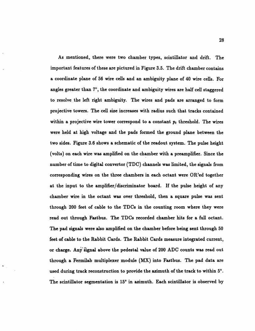
3.5 Schematic of the various chamber parts i.n the forward muon detector. 30
3.6 Schematic of the forward muon detector readout electronics. 31
3. 7 Efficiency as a function of gain for the FMU drift chambers. 37
3.8 Residuals for FMU + Jet with Jet Et > 10 Ge V. For each hit on
a track, the residual is the radial distance -from the measured hit
to the fitted track position. . 41
3.9 Residuals for Z0 candidates. 42
3.10 Uncertainty in Theta . . . . 44
3.11 Pad pulse height distributions. (a.) 1 x 1 tower centered on the
muon. (b.) 1 x 1 tower centered on azimuth opposite the muon.
(c.) 1 x 3 tower centered on the muon (d.) 1 x 3 tower centered
on azimuth opposite the muon. . . . . . . . . . . . . .
3.12 Geometric trigger acceptance for the NUPU 50% road.
46
48
•
•
Page 17
XVI
3.13 Vertex distribution m data. . . . . . . . . . . . . . . . . . . 49
3.14 Simulated vertex distribution for negatively charged muons . 50
4.1 Average smgle particle response (E/p) measured for hadrons m
the central calorimeter as a function of momentum. . . . . . . . . 60
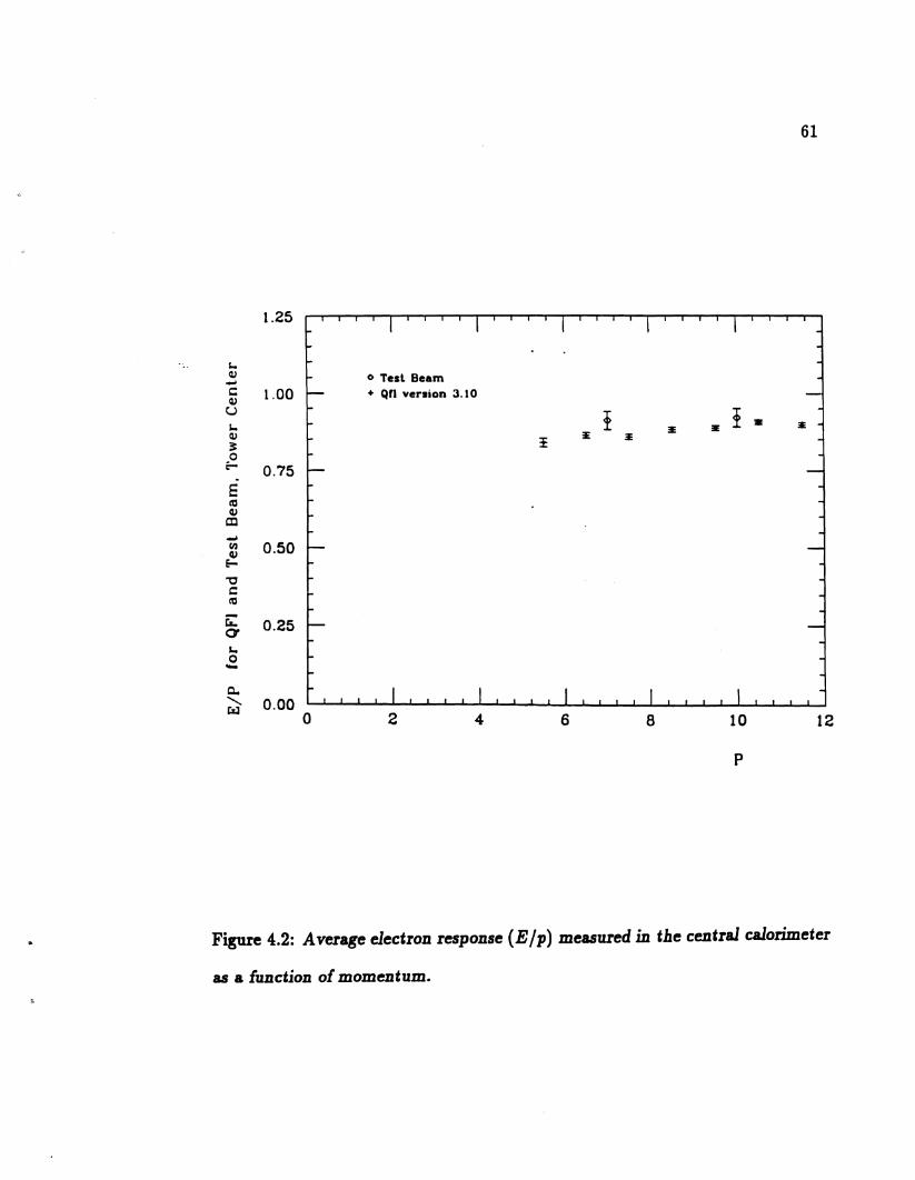
4.2 Average electron response ( E / p) measured m the central calorime-
ter as a function of momentum. . . . . . . . . . . . . . . . . . . . 61
4.3 Systematic uncertainty m the jet energy scale associated with the
uncertainty m smgle particle responses of pions and electrons, light
quark and gluon fragmentation, and the underlying event. . . . . 65
4.4 The observed and correct missmg Et parallel to the primary elec-
tron direction m conversion events as a function of the Et of the
primary electron. . . . . . . . . . . . . . . . . . . . . . . . . . . . 67
4.5 Photon - Jet balancing usmg events collected with the photon trig-
ger, El > 10 Ge V. . . . . . . . . . . . . . . . . . . . . . . . . . . 68
4.6 Photon - Jet balancing usmg events collected with the photon trig-
ger, El > 23 Ge V. . . . . . . . . . . . . . . . . . . . . . . . . . . 69
4. 7 Dijet balancing coordinate system m the plane transverse to the
beam direction. . . . . . . . . . . . . . . . . . . . . . . . . . . . . 72
4.8 Dijet balancing with central jets; longitudinal and perpendicular
kt fractions. . . . . . . . . . . . . . . . . .
4.9 Jet resolution as a function of jet energy.
72
74
Page 18
xvu
4.10 Momentum spectrum for particles in 10 to 12 Ge V jets compared
to that of 30 to 35 Ge V jets. . . . . . . . . . . . . . . . . . . . . . 75
4.11 Electron - jet balancing. The resolution from events simulated
with SETPRT+QFL agree well with the data. . . . . . . . . . . . 76
4.12 Missing Et projection fraction as a function of T/d measured with
dijet data in the ranges a) 50 GeV/c < :EPt < 100 GeV/c and b)
100 Ge V / c < :E Pt < 130 Ge V / c. . . . . . . . . . . . . . . . . . . 80
4.13 Missing Et projection fraction as a function of T/d after correction
for dijet data in the ranges a) 50 Ge.V /c < :E Pt < 100 Ge V /c and
b) 100 GeV/c < :EPt < 130 GeV/c.. . . 81
4.14 The MPF distribution for simulated jets. 82
4.15 The correction factor f3 as a function of jet Et for selected values
of T/d· • • ·• • • • • • • • • • • • • • • • • • • • • • • 83
4.16 Perpendicular Pt fraction for different T/d regions. 85
4.17 The separation in T/ between the simulated jet direction and the
vector sum of particle tracks which contribute to the jet. Low,
medium and high jet Et are between 10 Ge V and 20 Ge V, 20 Ge V
and 50Ge V, and above 50 Ge V respectively. . . . . . . . . . . . . 88
4.18 The' &Zimuthal separation between the simulated jet direction and
the vector sum of particle tracks which contribute to the jet. Low,
medium and high jet Et are between 10 Ge V and 20 Ge V, 20 Ge V
and 50Ge V, and above 50 Ge V respectively. . . . . . . . . . . . . 89 •
Page 19
..
XVlll
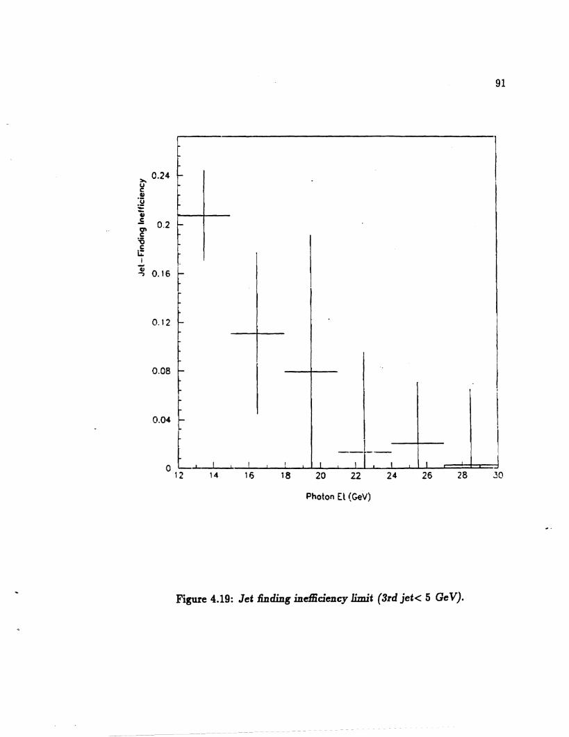
4.19 Jet finding ine:Riciency limit (3rd jet< 5 Ge V). . . . . . . . . . . . 91
5.1 Distributions of energy deposited in a 3 x 3 array of calorimeter
towers centered on the tower through which the forward muon was
thought to pass. . . . . . . . . . . . . . . . . . . . . . . . . . . . . 99
5.2 Ratio of positively charged muons to negatively charged muons as
a function of momentum. . . . . . . . . . . . . . . . . . . . . . . . 100
5.3 East versus West muon yield. The distributions are shown before
and after correcting for the detector e:Riciency on each end. . . . . 101
5.4 Muon speetrum from W bosons, bottom and charm quarks and
decay-in-flight prior to detector simulation. . . . . . . . . . . . . . 103
5.5 Momentum spectrum for inclusive forward muons compared to
simulated processes. . . . . . . . . . . . . . . . . . . . . . . . . . . 104
5.6 Rapidity distribution for inclusive forward muons compared to sim-
ulated processes. . . . . . . . . . . . . . . . . . . . . . . . . . . . 105
5. 7 Momentum spectrum for inclusive forward muons compared to the
predicted contributions from physics processes. The band shows
the upper and lower theoretical estimates. . . . . . . . . . . . . . 107
5.8 Rapidity distribution for inclusive forward muons compared to the
predicted contributions from physics processes. The band shows
the upper and lower theoretical estimates.
5.9 Charged particle spectrum at GDF . ....
108
109
Page 20
XIX
5.10 Ratio of positively charged muons to negatively charged muons as
a function of momentum in the muons in jets data sample. 112
5.11 Vertex distribution of the muons in jets data sample. . . . 113
5.12 The probability of x2 distribution for the muons in jets data sample.114
5.13 Number of wire bits in the octant containing the track. . . 116
5.14 Pulse height distributions for pads in units of ADO counts. 117
5.15 Plug electromagnetic and hadronic energy in the 3 x 3 array of
towers centered on the tower th.rough. which tb.e forward muon
passed. . . . . . . . . . . . . . . . .. . . . . . . . . . . . . . . . . . 118
5.16 Thansverse energy and rapidity distributions of both. jets in tb.e
muons in jets sample. . . . . . . . . . . . . . . . . . . . . . . . . . 120
5.17 (A) Muon momentum and (B) pseudorapidity distributions of tb.e
muons in jets sample. (0) P[el (D) 5R. . . . . . . . . . . . . . . . 121
5.18 (A) Opening azimuth.al angle between tb.e muon and tb.e opposite
jet. (B) Opening azimuth.al angle between tb.e muon and tb.e near
by jet. (0) Di:lference in pseudorapidity between tb.e muon and
tb.e near by jet. (D) 5R,.,-;et between tb.e muon and tb.e near by jet.122
6.1 Distributions of p~el normalized to unit area for tb.e di:/ferent pro
cesses which contribute to tb.e muons in jets data sample. No
tice th.at bottom quark processes b.ave a di:/ferent sh.ape than Hgb.t
quark processes. . . . . . . . . . . . . . . . . . . . . . . . . . . . . 135
Page 21
xx
6.2 Simulated bottom quark Pt and 11 distributions for events which
passed all analysis cuts. . . . . . . . . . . . . . . . . . . . . . . . . 138
6.3 Measured bottom production with the assumption that direct b
production represents the entire sample. . . . . . . . . . . . . . . 141
6.4 Measured bottom production with the assumption that gluon split-
ting b production represents the entire sample. . . . . . . . . . . . 142
6.5 Comparison of the measured and predicted cross sections for bot
tom production. The extreme modelling assumptions bound the
result on the horizontal axis. The real result lies somewhere be
tween the two. The measured result is higher than predicted for
all values of prin. . . . . . . . . . . . . . . . . . . . . . . . . . . . 145
6.6 Distributions of 1/opp normalized to unit area for the different pro
cesses which contribute to the muons in jets data sample. Notice
that quark processes have a different shape than gluon processes. 148
6. 7 The distribution of flopp in the bottom enhanced region, p~et > 2
Ge V, for the muons in jets data sample. . . . . . . . . . . . . . . 151
6.8 Momentum distribution for forward muons in GDF data displayed
with the result of the global fit in Table 6.8. . . . . . . . . . . . . 159
6.9 Pseudorapidity distribution for forward muons in GDF data dis
played with the result of the global fit in Table 6.8. . . . . . . . . 160
6.10 Corrected Et distribution for the jet near the muon in GDF data
displayed with the result of the global fit in Table 6.8. . . . . . . . 161
Page 22
XXl
6.11 Corrected. Et distribution for the opposite jet in GDF data dis-
played with the result of the global fit in Table 6.8. . . . . . . . . 162
6.12 The pseudorapidity distribution for the jet near the muon in GDF
data displayed with the result of the global fit in Table 6.8. . . . . 163
6.13 The pseudorapidity distribution for the opposite jet in GDF data
displayed with the result of the global fit in Table 6.8. . . . . . . . 164
6.14 The p~el distribution for GDF data displayed with the result of the
global fit in Table 6.8. . . . . . . • . . . . . . . . . . . . . . . . . 165
6.15 The azimuthal distance between the.muon and the opposite jet for
GDF data compared to the result of the global fit in Table 6.8. . . 166
6.16 The vertex distribution for GDF data compared to the result of
the global fit in Table 6.8. . . . . . . . . • • • • . . . . . . . . . . 167
6.17 The probability of x2 distribution for GDF data compared to the
result of the global fit in Table 6.8. . . . . . . . . . . . . . . . . . 168
6.18 The distribution of 5R between the forward muon and the nearby
jet for GDF data displayed with the result of the global fit in Table
6.8. . . . . . . . . . . . . . . . . . . . . . . . . . . . . . ~ . . . . . 169
6.19 The distribution of 54' between the forward muon and the nearby
jet for GDF data displayed with the result of the global fit in Table
6.8. . . . . . . . . . . . . . . . . . . . . . . . . . . . . . . . . . . . 170 .I
I
I
·1
I
I
I
I
I
I
Page 23
6.20 The distribution of 511 between the forward muon and the nearby
jet for GDF data displayed with the result of the global fit in Table
XXll
6.8. . . . . . . . . . . . . . . . . . . . . . . . . . . . . . . . . . . . 171
6.21 TI-ansverse momentum spectrum of b in simulated direct bottom
quark events which passed all analysis cuts. . . . . . . . . . . . . 174
6.22 The measured 1/ dependence of the cross section compared to the
theoretical prediction normalized to the central measurement. 187
6.23 Theµ scale dependence of the predicted cross section. . 188
A.1 Front, middle and rear plane chamber hit rates. . . . . . . . . . . 200
A.2 The rates for the first 420. nb-1 of the run compared to the average
rate. . . . . . . . . . . . . . . . . . . . . . . . . . 202
A.3 Average wire hit rates for each run and octant. 203
A.4 Average wire hit rates for each run and octant. 204
A.5 The elli.ciency calculation compared to data yield as a function of
octant. . . . . . . . . . . . . . . . . . . . . . . . . . . . . . . . . . 212
C.1 Comparison of the MNR and ISAJET cross section calculations to
the published NDE cross section. . . . . . . . . . . . . . . . . 219
C.2 '.lransverse momentum distribution for central bottom quarks. 220
C.3 Gluon splitting production bottom quark momentum correction
function. . . . . . . . . . . . . . . . . . . . . . . . . . . . . . . . . 221
Page 24
xxiii
C.4 Comparison of the MNR and ISAJET cross section calculations
for p~ > 20 Ge V. . . . . . . . . . . . . . . . . . . . . . . . . . . . 223
C.5 Comparison of the MNR and ISAJET tran~verse momentum dis
tributions for 1.9 < l11bl < 2.4. . . . . . . . . . . . ; . . . . . . . . 224
D.1 The azimuthal difference between the b quark and both the b quark
and the gluon. . . . . . . . . . . . . . . . . . . . . . . . . . . . . . 227
D.2 The transverse momentum distribution for three partons in bottom
events. . . . . . . . . . . . . . . . . . . . . . . . 228
D.3 Distribution of 'f/opp for either the b or the gluon. 231
D.4 The azimuthal difference between the b quark and both the b quark
and the gluon for 1.9 < 17/bl < 2.5. . . . . . . . . . . . . . . . . . . 233
D.5 The transverse momentum distribution for three partons in bottom
events with 1.9 < l11bl < 2.5. . . . . . . . . . . . . . . . . . . . . . 234
D.6 The weighting function applied to the ISAJET simulation so it
models the NLO calculation more closely. . . . . . . . . . . . . . . 235
Page 25
Chapter 1
Introduction
The Collider Detector at Fermilab (CDF) is used to examine particle interactions
produced at the largest center of mass energy currently generated in any labora
tory. These interactions are described by the mathematical theory known as the
Standard Model. Testing the predictions of this model is currently the primary
task of the CDF collaboration. To this end, this thesis measures bottom quark
production in proton - antiproton collisions and compares it to the prediction
from the Standard Model. This is the first measurement of bottom quark pro
duction in the forward region of the detector and therefore the first comparison
with theory in this region.
Bottom quarks decay via the electroweak interaction into a charm quark and
a W boson. The W boson can decay to either a pair of quarks or leptons. The
charm and any other light quarks usually decay hadronically into a jet of particles
1
Page 26
2
which are detected by the calorimeter. When the W boson decays to a pair of
leptons, one is a neutrino which goes undetected. The semileptonic decay mode
contains a jet from the decay of the charm quark and a lepton which can be
identified by the detector. In semileptonic bottom decays the lepton and jet are
usually within a few degrees of each other, therefore the lepton is surrounded by
some jet activity. This provides a way to distinguish bottom decays from the
decay products of gluons, which are the primary source of jets at CDF.
The central muon and electromagnetic detectors at CDF have a limited ac
ceptance for this signal since they require isolation for good lepton identification.
In the case of electrons, isolation is essential to distinguish between the jet en
ergy and the electron energy deposited in the calorimeter. For muons, isolation
is necessary due to the large "punch through" background from jets which are
not fully contained in the calorimeters and leak into the muon detector. These
central lepton tags have been used in other analyses.[!] The isolation requirement
is unnecessary in the forward muon detector (FMU) because the two meters of
steel in the toroidal magnets of this detector make the punch through background
negligible. The primary background to prompt muons observed with the FMU
detector results from pion and kaon decay-in-flight between the interaction point
and the calorimeter face.
The FMU subsystem of the CDF detector is located in the pseudorapidity
region from 1.9 < l7Jdl < 3.0. Detector pseudorapidity is defined as:
1/d = -ln(tan(9/2)) (1.1)
Page 27
\.
3
The bulk of FMU events contain muons with momenta transverse to the beam.line
between our trigger threshold of 5 Ge V and about 40 Ge V. The inclusive muon
spectrum in this momentum region is difficult to analyze due to copious quantities
of isolated pions and kaons which decay-in-flight. This spectrum is described by
known physics processes, but not conducive to a good measurement of bottom
quarks. To enhance the bottom content relative to the background, the presence
of a jet near the muon is required.
The data sample consisting of events with muons which a.re accompanied by
a nearby jet with corrected energy, Ef°" > .10 GeV, has a smaller background
fraction than the inclusive FMU event sample. A schema.tic representation of
dijet events where one of the jets contains a muon is shown in Figure 1.1. The
additional requirement of a substantial a.mount of energy in the calorimeter en
sures that events are the result of a harder scattering process than the muon alone
can assure. Even though the primary constituents of jets are pions and kaons,
the signal and background can be separated by kinematic features related to the
large mass of the bottom quark. The large mass tends to broaden the spatial
distribution of the decay products, therefore jets from bottom quarks are, on av
erage, broader than those from lighter quarks. Some ambiguity results, however,
when a gluon ~plits into a qua.rk-antiquark pair and the two partons remain near
each other in the detector. Since there may be some shared energy between the
two jets, the exact position of the quark, which decayed into a lepton, can't be
reconstructed. These, "gluon splitting" events can be distinguished from the "di-
Page 28
4
rect" bottom events by their topology. When two quarks are produced directly,
they tend to be correlated in 17, whereas those from gluon splitting tend to be
uncorrelated in 17. Using these kinematical features of lepton and jet events, this
analysis will measure the fraction of events attributed to bottom quark decays
and then the fraction of events attributed to direct bottom quark decays. The
measured number of events in the data sample attributed to all or direct bottom
quark decays will then be turned into the measured cross section by accounting
for the efficiency and acceptance of the detector, trigger and analysis cuts.
1.1 Direction and overview
This analysis depends on both the calculation of the theoretical bottom cross sec
tion and the complete understanding of the experimental apparatus. Therefore,
chapter 2, will describe the theoretical framework for calculating bottom quark
cross sections followed in chapters 3 and 4 by the features of the forward muon
detector and calorimeters. The data selection and checks on the performance
of the forward muon trigger and efficiency are presented in chapter 5. Finally,
the extraction of the measured bottom quark cross section will be presented in
chapter 6 followed by a discussion of the systematic effects which affect the result.
Page 29
~ ¢jet 2, muon
y
x
I I
I
)J
jet 1
muon \ \ \ \
I I 1- - - - - - - - - --->-I . jet 2 I
5
z
Figure 1.1: Scbematic representation of dijet events w.bere one oft.be jets bas a
muon nearby.
Page 31
Chapter 2
Theory and Background
The production of bottom quarks from collisions between protons and anti
protons is described by Quantum Chromodynamics (QCD). The exact solutions
of QCD are complicated and have not yet been found. Only perturbative solu
tions exist and these are usually expressed as the sum of a series of terms. For
most purposes, these series solutions are truncated after the leading or next-to
leading order terms. Recently, the next-to-leading order (NLO) calculation of
the heavy quark cross section has been worked through completely and com
pared to measurements at CERN and Fermilab. The following sections describe
the leading order calculation and issues involved in extending the calculation to
next-to-leading order. The results of previous measurements and their implica
tions are also discussed.
6
Page 32
2.1 Calculation of QCD cross sections at
leading order
7
There are a limited number of topological ways at each order of a 8 to connect two
incoming partons to make bottom quarks. Feynman diagrams of the leading and
next-to-leading order interactions are shown in Figure 2.1. Each vertex carries a
factor of ..;a;, the coupling constant of the strong force. Since the leading-order
diagrams contain two vertices, and the square of the number of vertices enters
the cross section, these interactions are of order 0( a~). The next-to-leading order
interactions with three vertices are of order O(a!). Since a 8 is smaller than one,
higher order terms may be neglected. Unfortunately, we have learned that a 8 is
not sufficiently small to make the series converge at just leading order. Even at
next-to-leading order there is evidence that the series is not fully convergent, but
a higher order calculation is not yet available. At each order of a 8 one can write
down the predicted cross section, iT, which is called the parton cross section.
It should be noted that the next-to-leading order diagrams in Figure 2.1 con
tain either three or four vertices. It has already been mentioned that ..;a; con
tributes to the cross section as the square of the number of vertices. There are,
however, interference terms between diagrams at different orders which also con
tribute. The product of a lowest order diagram with a next-to-leading order
diagram contributes at 0( a~/2 ) or 0( a~). These interference terms are clearly
not of the same order, but the calculation retains all terms at 0( a~).
Page 33
8
I I •
I q s-channel,, b u-channel t-channel I leading order
cr>"<b direct production
g~b g 'TITr\...-b g:J><b '
g.... b g~b g b
q
next-to-leading order q~g b
radiative corrections ~~~ to leading order q b diagrams
g"' ~b .,, .... ~ g
::;<~ _..,
-".; g~b g b _,~::~ 'Z:'.!.' g
g"'· 'b &~b g b
g ""!TTT'- b g:p<b "Tn'I" g
g~b g b
gluon splitting
~x~ q qb
" diagrams g~b q g b
cr < g 1 '5bdB)d81Si'g b = ~_, -
g~~ g~~--"~,~-Y" b
..... " g~ "~ 0 ,.,....... g b g
:::
t1avor excitation q q q q
= = diagrams b ,. -
u g·m•~~ 0 '
-------b g • 11111111 &iii' er gr iihhl) iili\g ,. = .. g•nn~b-
E -g ..... ~:
b
examples of q~~ q nm b ~=r:J><b virtual corrections I I -to leading order q b Cf--~b q b
diagrams .... g~~ g:a=b- g::b<b
g b g b g b
Figure 2.1: Leading and next-to-leading order bottom production diagrams.
_ _J
Page 34
initial q or g
spectators hadrons from fragmentation
>---
parton subprocess
final state partons
9
Figure 2.2: In proton-antiproton collisions, the partons (quarks and gluons) inside
tb.e parent particles interact. All leftover partons interact minimally and are
th.us called spectators to tb.e interaction. T.b.e parton subprocess is one of tb.e
interactions from t.b.e previous figure.
Since the initial state is composed of quarks and gluons which are part of the
proton or antiproton, they are not truly independent as the diagrams in Figure 2.1
assume. Figure 2.2 demonstrates the concept of proton-antiproton interactions
in the spectator model. Here, we assume that the partons in the proton and
antiproton interact independently. This approximation becomes more realistic as
the collision energy is increased.
In order to calculate the cross section for bb quark production in proton-
Page 35
10
antiproton collisions, the parton cross sections, iT, must be convolved with the
momentum spectrum of the initial state partons and summed over all possible
initial states. The parton momentum distributions in the proton and a.ntiproton
are described by structure functions which are found empirically. EHLQl struc-
ture functions are shown as an example in Figure 2.3, where :c is the fraction of
the proton momentum carried by a particular parton. The cross section is then
calculated as:
<Ttot(P P -+ bb + X) = L fl fl d:cid:c;J(:c;)J(:ci)iT(pip; -+ bb + X) (2.1) i,; Jo Jo
where P(P) are proton (antiproton) momenta., b(b) are bottom (antibottom)
quark momenta, p are parton momenta, ir(PiP; -+ bb + X) is the parton level
cross section and the sum over i and j represent the sum over all possible partons
in the proton. By inserting the parton cross sections for the diagrams in Figure 2.1
into this integral, we can predict the expected yield of bottom quarks measured
by the experiment.
The cross sections, ir, are crucial to the total cross section, and are found from
the QCD theory. The lea.ding order calculation is easy to summarize. Strong
interactions are described by the group, SU(3).[2] This is a non-abelian gauge
group which defines the QCD Lagrangian:
L = -~F:vFaµv + i[J;(i'Y,,Djk - M;k)'i/Jk (2.2)
where the indices a,j and k refer to color. The color couplets range from a =
1, ... , 8 and there are three color charges in the theory; j, k = 1, 2, 3. The covariant
Page 36
11
1.0
0.8 .
......-.. 0.6 \~ ~ .._
'+--. 0.4 H
0.2
0.0 0 0.2 0.4 0.6 0.8
x
Figure 2.3: The distribution functions, f ( z ), represent the probability of :finding
a quark with momentum fraction :z: = p/ Pproton between :z: and :z: + d:z:. The
distribution functions are shown for tb.e up, down and sea quarks witb. tb.e gluon.
For t.l.Us plot, EHLQl structure functions were used.
Page 37
12
derivative D is defined to maintain local gauge invariance.
(2.3)
where G~ are the gluon fields, Ta are the SU(3) generators, and g is the strong
coupling. M;k is the quark mass matrix. The gluon field tensor is
(2.4)
where fabc are the constants defined by the commutation of the SU(3) generators.
The SU(3) commutation relation is:
(2.5)
The Lagrangian contains quark-gluon and gluon-gluon self interactions. The
diagrams in Figure 2.1 contain such interactions. At first order, all the diagrams
are tree level, and the calculation of the cross sections is straight forward. For the
process cr(ab--+ cd), it is customary to define the Mandelstaam variables:[2, 3]
i =(Pa - Pc)2
ii = (Pa - Pd)2
(2.6)
(2.7)
(2.8)
where the four vector of each particle is denoted by p,,.. Then the cross section is:
dcr/di(ab--+ cd) = IMl2 /(167rs2 ). (2.9)
Table 2.1 lists all the matrix elements, IMl2 for the first order heavy quark and
gluon production processes.[2]
Page 38
13
I part~n subprocess II IMl2 / g!
qij--+ QQ 1 i2t;u2 9 j
gg--+ QQ l u2 ·t;,i2 - !! u21p a ut s •
qij--+ gg 32 u21;.i2 _ ~ "2;~i2 21 ut 3 •
gg--+ gg ?C 82~u2 + 82JP + u28tp + 3)
qg--+ qg £.#- 4 92+u2 t - 9 ua
Table 2.1: Lowest order heavy quark production matrix elements.
2.2 Extension of QCD cross sections to
next-to-leading order
There are two complications which must be handled carefully when extending the
leading order calculation to higher orders. First, one must adopt a regularization
procedure that renormalizes any integrals that are infinite. To first order, the 1/u
and 1/i terms are infinite only when the final state has no observable Pt· Since
these limits are not observable, the calculation can be cut off to eliminate these
regions of phase space without affecting the observed cross section. At the next
order, the divergences occur when the energy of the emitted gluons is zero or the
opening angle· bf a vertex in the event is zero. With three final state partons,
the first two can be produced with observable rapidity and momentum at the
same time that gluons with diverging probability are produced. Thus, for three
final state partons, the divergences affect the cross section for observable events.
Page 39
14
Divergences from soft radiation, when properly regulated cancel between real
and virtual graphs. Collinear divergences must be factorized later. A fractional
space-time dimension (D = 4 - 2e) is introduced to express the matrix element
as a finite quantity. The matrix element is then expanded into a series which is
valid for small e and the series is terminated at O(e).
The second complication to a NLO theory is in defining which partons are
part of the proton and which are the result of hard interactions. Perhaps a better
question is: exactly what distinguishes a hard scattering from the proton internal
interactions? There are two schemes which. are appropriate to next-to-leading
order calculations, DIS and MS. Both of these distribute the radiative corrections
between the structure functions and parton cross section in a consistent way.
Although the two schemes are not interchangeable, conversions from one to the
other exist. In this analysis, the MS scheme was used. Next-to-leading order
structure function definitions lead to "scheme" dependent definitions of a,,, and
fr. Specifically, a,, becomes a function of µ.2 where µ. is a scale factor on order of
the energy exchanged in the interaction. Since u, i, and 8 diagrams contribute
to a single cross section, the definition ofµ. is not exact, but the calculation is
expected to remain constant over a large range of µ. values.
There are two main sources for the NLO calculations. Nason, Dawson, and
Ellis (NDE) have published the single particle inclusive cross section and dif
ferential cross sections with respect to momentum and rapidity for heavy quark
production.[4] Mangano, Nason, and Ridolfi (MNR) realized the need for fully
Page 40
15
differential cross s~ctions and have made a computer code available to the CDF
collaboration which calculates these.[5] The first is sufficient to compare to in
clusive bottom cross section measurements. The second allows for the study of
correlations between the three final state partons.
2.3 Status of bottom quark cross sections
The inclusive cross section for bottom quark production at central rapidities has
been measured and compared to the NDE theory. Figure 2.4 shows the compari
son of all CDF measurements, ( y'S = 1.8 TeV) , with the NDE prediction.(6]
Clearly the measured points lie above the theoretical band. Note that the
measured cross section at UAl, shown in Figure 2.5 where the center of mass
collisional energy is smaller ( y'S = 0.63 Te V) agrees well with the theoretical
prediction.(7] The publication of the CDF measurements has caused doubts about
the NLO calculation. Ellis. claims that the NLO theory is flawed.(6] The NLO
calculation turns out to be a strong function ofµ., the scale factor. The depen
dence of the cross section on µ. is a large part of the uncertainty in the theoretical
prediction. However, theµ. scale dependence is a symptom, not the real effect.
The reason for the discrepancy is due to the fact that y'S >> m >>A at CDF.
In this particular limit, the perturbation series is no longer an expansion in a 6 ,
but rather a 6 ln(s/m2 ) and therefore does not converge. As yet, an improved
theory in this particular kinematic region has not been worked out.
Page 41
I ,
I
I -
!-
I
1·
->< ..Q
t Q.,
IQ., -
0
pp -- bX
Nason. Dawson, Ellis m 11 •4.75 CeV. A 4 -260 MeV. DFLM. /.J.o .. v(m9Z+PTZ) 4.5<m 11 <5CeV. 160<A4 <360MeV, µ.o/2<µ.<2µ.o
CDF Preliminary 1988- 1989 data
There are correlated uncertainties among the measurements
.....
10 20
PTmin [GeV /c]
30 40
I
16 I
Figure 2.4: Tbe b quark production cross sections measured using electrons as
well as other GDF measurements and tb.e QCD prediction by NDE.
Page 42
,......... ..0 :i. .........,,
_.._ 10 c e
I-
0..
/\ 1 I-
0.. '-"' b
-10
-10
-10
-10
0
pp --1- b + X, lybl<1.5 • dimuons, muons from different quarks • dimuons, b chcin decoys * dimuons, b ~ J/1/1 decoys • sirigle muo!"'s, b --1' µ. X
- O(a.3) OCO, Nason et al., µ.,•v'(m_,2+py"11112),
m-.=4.75 GeV/c2 , A4 =260 MeV, OFLM str.f. -····· µ.,/2<µ.<2µ.,, 4.5<m-.<5 GeV/c2
160<A4 <360 MeV I
17
10 20 30 40 50 60 Pr min (Ge v I c)
Figure 2.5: The b quark production cross sections measured at UAl with the
QOD prediction by NDE.
•
Page 43
18
There are other possible explanations that are being investigated to account
for the discrepancy. Since the gluon distribution was measured at lower energies
and extrapolated to CDF energies, it is possible to modify the shape of this dis-
tribution while maintaining consistency with available measur.ements of structure
functions in such a way that it increases the predicted cross section at CDF.[8]
While this may account for part of the discrepancy, it has already been shown
that the structure function cannot be modified enough to account for all of it.
Finally, all the measurements at CDF are correlated. The Peterson fragmen-
tation model is used to evolve the bottom quark into a bottom meson with the
appropriate momentum spectrum. This model has a free parameter which was
measured by CLEO [9] and is used in all the CDF measurements. If there are
any uncertainties in this model, they feed into all the measurements identically.
So, there could conceivably be a shift in all the CDF bottom quark cross section
measurements due to the dependence on a single fragmentation model.
2.4 Motivation for the measurement of direct
bottom at forward 1/ ....
The forward muon bottom tag is unique in that it will give information about
the 1/ dependence of the cross section. Theory predicts that the cross section
drops off at high 11, but the exact shape of this drop has not been measured. The
magnitude of the drop off is related to the mix of LO and NLO diagrams. Hence,
Page 44
19
the forward region is of particular interest.
Another feature of the forward measurement is that it specifically requires
jets in the events and therefore the correlations between different partons can be
compared. In particular, the mix of diagrams that look topologically more or less
like LO and those that are NLO may be compared. Since the LO calculation with
small radiated gluons is far more stable with respect to the µ. scale, it is possible
to see whether the discrepancy between theory and measurement persists without
the calculational source of uncertainty from the perturbation theory.
•
Page 45
Chapter 3
Forward Muon Measureinent
The Collider Detector at Fermilab (CDF) is designed to measure the momentum
and energy of electrons, photons, muons, hadrons and jets. The forward muon
(FMU) detector is one component of the CDF detector. In this chapter, I will
describe the experimental facilities at Fermilab, and the detector components
used in the identification and momentum measurement of forward muons. In
addition, I will present the FMU detector efficiency, resolution, luminosity, and
trigger efficiency which defines the quantity and quality of observed muons.
20
Page 46
21
3.1 Overview of the experimental facilities and
the Collider Detector at Fermilab(CDF)
The accelerator at Fermilab consists of several stages of particle acceleration to
reach the final collision energy of 900 GeV in each beam. Figure 3.1 shows the
general layout of the accelerator. First, n- ions are produced in a Cockroft
Walton Generator. The ions are injected into a linear accelerator where they
reach an energy of .5 Ge V. In a booster ring the electrons are stripped off the
ions which become bare protons and are then.accelerated to 8 GeV. Next the pro
tons are injected into the Fermilab Main Ring which is a proton synchrotron with
radius 1 Km. Here they are accelerated to 150 GeV. To obtain proton-antiproton
collisions, the first protons are used to make antiprotons. Antiprotons are created
when protons from the main ring are smashed into a tungsten target. The an
tiprotons are stored and stochastically cooled in an accumulator ring until there
is a stack of sufficient size to make a high luminosity beam. Then six bunches
of protons and another six bunches of antiprotons are injected into the Tevatron
where they are accelerated in opposite directions to 900 GeV. As viewed. from
an airplane, the protons travel clockwise around they ring, and the antiprotons
travel counterclockwise. The bunches meet each other 6 times as they travel once
around the Tevatron.
The Collider Detector at Fermilab (CDF) resides at BO, which is one of the
six points where the Tevatron Beams collide. It uses a combination of tracking
•
Page 47
Debuncner and Accumulator
p extract ;t Inject
,...----Tevatron
LINAC
._ Booster
BO (CCF)
Switcnyard
Figure 3.1: Overhead view of tbe Fennilab accelerator complex.
22
Page 48
23
chambers and calorimeters to measure the momentum and energy of particles
created in proton-antiproton collisions. It is designed to give the four-momenta
of all possible leptons and jets, which are the general features of high energy
events. Figure 3.2 shows the layout of the detector. It has a cylindrical symmetry
surrounding the Tevatron beam pipe. Coordinates for the collider are defined such
that the Z axis i.s aligned along the proton direction at the interaction point. The
X axis points away from the center of the Tevatron Ring, which leaves the Y axis
pointing up out of the ground. X 0 , Yo, Z0 is defined to be the center point of
the detector. This convention will hence forth be referred to as CDF coordinates.
In the central region the detectors are layered like an onion, with the Vertex
Detector adjacent to the beam pipe followed by the Central Tracking Chamber.
The 1.5 Tesla superconducting solenoidal magnet surrounds this to provide the
bend of charged particle tracks necessary for the momentum measurement. Next,
an electromagnetic (EM) calorimeter and a hadronic (HAD) calorimeter measure
the electron and jet energies. Finally, muon chambers are mounted on the exterior
of the detector.
In the forward region, from about 8 < 30°, the endcaps of the solenoid are
layered away from the vertex with the Plug Calorimeters (EM and then HAD).
For the far fo~ard region which is not covered by the Plug Calorimeters, the
Forward Calorimeters are used. Finally, behind this resides the Forward Muon
Detector (FMU).
The detector components used in this analysis are the Forward Muon Detec-
•
Page 49
~--- .. IL::Ml . .IL _. -- ---- -
I -- B.-{4011. . • . · - .. --·-----·-... i
ELEVATION VIEW LOOKING SOUTH
Figure 3.2: Side view of the ODF detector.
·..:.: "--'"~-- -~ii.FERcoNJuc:TINO COi.
csmw. DAFT l\.llES TAAO<Hl !
INlERACTION ~l
-./.-~-':- , VERTEK TPC"S
I EN>PLUO EM -- i SHOWER~ER .-L.--.Jl!lo_....,._"'!'
_:;. - --
n -1oe11. ~
I"'
Page 50
25
tor, the Central, P_lug and Forward Calorimeters, and the Vertex Detector. These
devices provide us with enough information in each event to measure the vertex,
forward muon momenta, and jet energies. The rest of this chapter details the
measurement of muons in the forward detector. The next chapter describes the
measurement of jets.
3.2 Forward Muon Detector components
The Forward Muon (FMU} Detector is a muon spectrometer in the small angle
region at CDF as shown in the cutaway schematic of Figure 3.3. At each end
of CDF there are a set of toroidal magnets (1.6 to 2.0 Tesla field strength) with
planes of drift chambers in front, between, and behind. In the front and rear
planes a scintillator plane is sandwiched between the drift chamber and the toroid.
Each plane consists of 24 chamber wedges as shown in Figure 3.4. The scintillator
chambers were abutted into position whereas the drift chambers were mounted
so they overlapped. Thus, the active volume of the scintillators contained small
gaps near the wedge boundaries whereas the drift chambers had no gaps. The
specific design parameters for the chambers as well as the survey procedure may
be found elsewhere. [10, 11] Instead of concentrating on previously documented
dimensions and construction materials, I will describe the general detector design
schematically. With this approach it is easier to understand the diagnostic checks
for the system which were used during the run and later oflline with data.
Page 51
- ':::::- x --... )-, -- -- - y -A " s toroid toroid -~ - - - ---32° -- -............ - beam line ---------toroid c toroid s ------ S = scintillation chambers -- (counters)
- C, A = coordinate and ambiguity - filiddle f ~nt sides of the drift chambers
-i{f =e pane pane
Figure 3.3: Side view of the Forward Muon Detector. The detector is symmetric
about the vertex.
Page 52
Octant 3
Octant 4
Octant 2
...... -- -
Octant 5
t"- (") - :r '- ~ Ill 3 .c E ~ ~
.., ..c: -u 00
Octant 1
/
- -
Octant 6
z
27
y
)-x
Octant 0
Octant 7
Figure 3.4: Each plane consists of 24 chambers each of which spans 15° in az-
imutb.
•
Page 53
28
As mentioned, there were two chamber types, scintillator and drift. The
important features of these are pictured in Figure 3.5. The drift chamber contains
a coordinate plane of 56 wire cells and an ambiguity plane of 40 wire cells. For
angles greater than 7°, the coordinate and ambiguity wires are half cell staggered
to resolve the left right ambiguity. The wires and pads are arranged to form
projective towers. The cell size increases with radius such that tracks contained
within a projective wire tower correspond to a constant Pt threshold. The wires
were held at high voltage and the pads formed the ground plane between the
two sides. Figure 3.6 shows a schematic of the readout system. The pulse height
(volts) on each wire was amplified on the chamber with a preamplifier. Since the
number of time to digital convertor (TDC) channels was limited, the signals from
corresponding wires on the three chambers in each octant were OR'ed together
at the input to the amplifier/discriminator board. If the pulse height of any
chamber wire in the octant was over threshold, then a square pulse was sent
through 200 feet of cable to the TDCs in the counting room where they were
read out through Fastbus. The TDCs recorded chamber hits for a full octant.
The pad signals were also amplified on the chamber before being sent through 50
feet of cable to the Rabbit Cards. The Rabbit Cards measure integrated current,
or charge. Any· signal above the pedestal value of 200 ADC counts was read out
through a Fermilab multiplexer module (MX) into Fastbus. The pad data are
used during track reconstruction to provide the azimuth of the track to within 5°.
The scintillator segmentation is 15° in azimuth. Each scintillator is observed by
Page 54
29
four phototubes, whose outputs are OR'd together to improve the light detection
efficiency.
Diagnostics for many parts of the system were included in the design. On
each scintillator was mounted an LED which co~d be pulsed through Fastbus
and read out through the normal data path. In addition, by turning off the
voltage to all of the phototubes except one in a chamber, each phototube could
be tested individually, thus fully verifying its operation. The diagnostic for the
wire chamber consisted of a wire which ran the length of the chamber and coupled
capacitively to the sense wires in the chamber. When the long wire was pulsed,
the signals would follow the normal data path and be recorded in the TDCs.
To check that the chamber gain was high enough, Fe55 sources were mounted
in four chambers in each plane. Each chamber contained a variety of cell sizes,
each necessitating a different voltage. One cell of each size was monitored with
the Fe55 source. The gas-gain system used the signal from the Fe55 source to
diagnose overall gain problems.
The FMU trigger used the projective tower geometry of the drift chambers
to search for patterns of wire hits likely to be high Pt tracks. The front cham
bers were smaller than the middle chambers which were smaller than the rear
chambers. In principle, a straight line connecting the same cell number in all
three chambers also included the vertex. The actual chamber positions during
data taking were not perfectly placed in Z and therefore only approximated the
ideal configuration. Tracks that emanated from the event vertex and traversed
Page 55
cell -divider
----------------------------= """"- - -------
W··~ - - - - -~~ - - - - -· ._ --------------------~-----
---- ---- ---------------..., ______ _ 1-------.... -- - - - - ---------"----- ---------~------------..... --------------------------------------._ _______ _ ---------I'-- -- - -·
Coordinate Wires l - 56
.._ - - -
.... _ - -.... -.... t
- - - -t - .... - - - -- - - -
""" - - - ---- ... ------... - -"""'"'-----------
'"- - - - - - ' ._ ______ , "-------------------~--------------.,. __ _
L- - - -Jo-------~-------L.-------------------------------------------------------------------------
l- - - - - - - - - - '
Ambiguity Wires 57 - 96
I I I 1"1 I I
I
1
l I I
·-
Cathode Pads
fm~~-light guide
_ _.._photo lube
Scintillator Wedge
Figure 3.5: Schematic of the various chamber parts in the forward muon detector.
Page 56
Components on: Chamber
WIRES
preamp
PADS
SCINTILLATORS
4 PMT phototubes
PMT per chamber
PMT
PMT
Components in: Components in: Collision Hall Counting Room
Clear from Pucker
TDC
(96 channels) Amplifier/ 96 oclant services LI Discriminator wires
Clear from CD.F trigger
Rabbit Card
attenuator {Integrates charge)
1 octant Trigger
MEP Fastbus readout
Clear from Pucker
STRUCK LATCH
Fastbus readout
Ll Trigger
Figure 3.6: Schematic of the forward muon detector readout electronics.
31
Page 57
32
all three chamber planes without deviating by more than a chamber cell were
deemed to have large Pt· The wire hits were sent to the trigger boards through
the TDC auxiliary fastbus connector which is located on the back plane of the
Fastbus crate. Although test programs were written to test the different modules
in the trigger itself, the back plane jumpers between the TDCs and the trigger
boards were not tested after they were installed. A sample of these jumpers were
tested in place after the run and found to contain (2.9± 1.1)3 broken connections
which accounts for the Level 1 trigger electronics efficiency. The trigger resided
in the counting room Fastbus crates which made it easy to set trigger inputs and
read back the expected triggers ..
A complication of analysis with the FMU trigger is that both the trjgger and
chamber configuration changed during the run. Two different Level 1 trigger
boards were used. The first FMU trigger used Half-Octant Pattern Units or
HOPU boards. Each HOPU contained the logic to analyze the wire hit informa
tion from an octant in q, and 7° to 16° in 8 to determine whether a muon had
passed one of three Pt thresholds defined by the hit pattern. The Pt threshold
used to select the data was satisfied by a simple coincidence of hits in the same
coordinate-wire cell number in each of the three chamber planes. In other FMU
documentation, this is referred to as the 1003 trigger.
The original HOPU trigger, consisting of a coincidence between 3 coordinate
wires, yielded an unacceptably large rate. To solve this problem, a temporary
DIHOPU trigger was installed covering the range 7° to 16°. Two HOPUs were
Page 58
33
used for each octant wedge with one HOPU searching the coordinate plane wires
and the other HOPU searching the ambiguity plane wires. A valid DIHOPU
trigger required a 3-wire coincidence among coordinate hits and also a 3-wire
coincidence among ambiguity hits. The two coincidences were not required to be
satisfied in the same octant, however. Again, all HOPU thresholds were set at
the 1003 level in FMU terminology.
In the final trigger, the 3 coordinate wires were required to line up both
in 1/ and </>( 45°) with the 3 ambiguity wires. This was achieved with a new
trigger board that searched for a 6 wire coincidence within one octant. One
New Octant Pattern Unit, called a NUPU, replaced both the coordinate and
ambiguity HOPUs covering the angular range 7° to 16°. The main difference
between the DIHOPU and NUPU triggers was that the latter was more efficient
at selecting real muons, thus reducing the trigger rate. The NUPU Pt threshold
chosen required stiffer tracks than the other thresholds available and is referred
to as the 503 threshold in the FMU documentation.
The other detector change was the result of an HV accident which occurred
during December 1988. Since many channels were disabled, Fermilab allowed
the Wisconsin group access to remove a large fraction of the chambers with
their associat~d .. electronics and fix them. The chambers and electronics were
arranged differently in the system when reinstalled. Therefore, the luminosity
and efficiency calculations require separate treatment for the data taking periods
separated by these changes in FMU configuration. '
Page 59
34
Events passing the hardware trigger were passed to an event processor (Level
3) which ran the event reconstruction algorithm on the events. If a reconstructed
muon could be found with either 5 or 6 hits, the event was written to a data
tape.
3.3 Luminosity for the FMU trigger
The luminosity that CDF was able to write to tape during the 88/89 run was
( 4.4 ± .32) pb-1 • The CDF luminosity on the data tapes used in this analysis
was (3.63 ± .25) pb-1 which is lower because some tapes were unreadable and
there was a period where the FMU voltage was turned oft' around the time of
the Christmas repair.[12, 13, 14] These numbers have been calculated tape by
tape and reflect multiple interaction corrections. The FMU trigger was limited
to a constant rate of .1 Hz, therefore any trigger which came in closer than 10
seconds after the previous accepted trigger was automatically rejected. Since
trigger rates scaled with the luminosity delivered by the accelerator, each run
had a characteristic rate and the amount rejected due to the rate limit varied.
For each data taking run, the CDF shift crew recorded trigger statistics with a
monitor program called L UMMON. The monitor summaries included the Level
1 cross section before and after the rate limit. The ratio of these numbers is the
average FMU prescale. The FMU luminosity is calculated by multiplying the
CDF luminosity by the FMU trigger prescale factor on a run by run basis. The
Page 60
35
RUNS TRIG I CDFLUM(nb-1 ) I FMULUM(nb-1 ) l R15880-R16566 HOPU 102.1±6.9 4.9 ± 1.9
R16567-R18199 DIHOPU 1345.2 ± 91.5 668.4 ± 63.2
Christmas Repair
R18685-R1884 7 DIHOPU 139.0 ± 9.5 92.1±6.7
R18848-End NUPU 2047.1±139.2 1037 .1 ± 70. 7
Total I 3633.4 ± 247.1 I 1802.5 ± 142.5 1
Table 3.1: FMU trigger configurations and associated luminosity for tb.e 1988/89
GDF run.
FMU effective luminosity corresponding to 3.63 pb-1 corrected for deadtime in
the 88/89 run is (1.80 ± .14) pb-1 • The error bar includes a 6.8% uncertainty in
the CDF luminosity, statistical errors from the Level 1 and Level 2 trigger scaler
values recorded in the LUMMON end of run summaries, and 5% uncertainty in
the rates assigned to a small number of runs missing LUMMON summaries. As
mentioned before, there were changes in the FMU configuration which require
separate treatment. Table 3.1 lists the luminosity for CDF and the FMU trigger
for time segments corresponding to different trigger conditions.
Page 61
36
3.4 Forward Muon Detector efficiency
The overall efficiency may be divided into two parts. The design efficiency for
the FMU system was very high. The actual efficiency, including occasional hard
ware failures, was somewhat lower. In general it can be shown that the system
performed at the design efficiency and that a small fraction of component failures
account for the degradation of this to the measured efficiency.
The gas gain system used Fe55 sources to monitor the gain of the chambers.
The signals from the Fe55 sources were read out through an emitter follower
attached to an alternative output on the preamplifier. As these signals were pro
duced on the chamber and monitored 200 feet away, a significant a.mount of at
tenuation occurred in the cable. The chamber HV was adjusted so as to maintain
an Fe55 pulse height of (200 ± 85) m Vat the monitoring station, corresponding
to 460 m V to 1140 m V as measured at the chamber output. For comparison, a
test setup was used to measure the chamber efficiency as a function of the size of
the source signals. Figure 3. 7 shows how the chamber efficiency depends on the
source signals. From this I conclude that the gas gain was high enough to collect
data with (99.6 ± .5)% efficiency, for channels in good working order. [13, 15]
Component failures consisted of broken electronic channels which affected
either a single chamber wire or the set of three chamb~r wires which were read
out together in a single TDC channel. These were estimated with the ratio of
5 hit to 6 hit tracks in the system. Since the chamber efficiency of the gas was
Page 62
1. 1
/\ ~ v 1. 0
A u c Q)
u ~ o. 9 ~
Q)
\... Q)
.0
E 0. 8 0 l: u
o. 7
37
I I I I I I
."T'.
• .I.'
~ Test Setup
x 88-89 Doto
0 200 400 600 800 1000 1200
Source Signal at EF <rnV>
Figure 3.7: Ef1iciency as a function of gain for the FMU drift chambers. •
Page 63
38
shown to be excellent, the missing hits in the 5 hit tracks were assumed to be
broken readout channels or wires in the chambers. Correlated failures, which take
out 2 or more hits on a track, were not accounted for with this technique. Failures
of groups of wires in both the coordinate and ambiguity plane occurred due to
broken HV connections, gas impurities (due to leaks in the wire chambers) or
problems with the power for preamps. A similar effect occasionally resulted from
TDCs which were temporarily disabled to mask "hot" trigger octants. These
failures were identified by occupancy observations, and were tabulated run by
run to account for inefficiencies. The detector efficiency has contributions from
the six hit chamber efficiency, Ece{6), the group failures, Egroupi and single non
functioning wire chambers, Eac·
f6 hit = Ece{6) X Egroup X Eac• {3.1)
The product of these efficiencies is calculated separately for the west, 'T/ < 0,
and east, 'T/ > O, ends of the detector. The efficiency of finding 6 hit tracks as
described in appendix A is { .570 ± .028) on the west and { .452 ± .023) on the
east. The average over east and west is (.511 ± .026). These efficiencies include
all types of component failure .
....
3.5 Forward muon momentum resolution
A detailed description of the tracking algorithm may be found elsewhere.[10, 16]
A least squares fit was performed using the vertex and 3 hit positions at each
Page 64
39
chamber plane. First a simple parabolic fit was made. Using the parameters
found in the parabolic fit as an input, the more complicated fit including multiple
scattering and chamber resolution was performed iteratively. The square root of
the diagonal covariance matrix elements for least squares fits are the uncertainties
of the fitted parameters.
The momentum resolution of the FMU system has three components. First,
there is a momentum uncertainty due to the fact that muons scatter in the
forward calorimeters and the toroids, thus hits are distributed about the ideal
track direction. This contribution is described by random walk statistics.[10]
Since high momentum tracks are scattered less than low momentum tracks, this
contribution is momentum independent, namely
AP/ P = .166 ± .004. (3.2)
The second contribution comes from the chamber resolution. When the elec-
trons shower in the gas to make a hit on the wire, there is an intrinsic resolution
to the pulse and readout electronics. The resolution of the hit positions was
measured in the data using the distance between coordinate and ambiguity hit
positions, corrected for the slope of the track. These distributions are shown in
Figures 3.8 and 3.9 for FMU + jet and Z events. The resolution of the chamber
is related to this distribution by
(3.3)
The resolution was therefore (672±61) µmin the Z events and (631±15) µ.min the
•
Page 65
40
FMU + jet events. Since the momentum resolution does not depend critically on
the exact value of the position resolution and there could be systematic differences
between different data samples, a round number of 650 µm was used. A test setup
was used to study the chamber resolution and it was found that the chambers by
themselves have ( 450±50) µm resolution. The difference between this number and
the resolution measured in the CDF data has been accounted for by chamber to
chamber variations in wire spacing, t0 , drift velocity and gain variations coupled
with gain dependent time slewing in the amp/disc cards.[13] Simulated tracks
with hits smeared by a gaussian of width 650 µm were found to have a momentum
resolution of
AP/ P = (.0015 ± .0003) x P (3.4)
The third contribution comes from uncertainties in the chamber positions
from the survey. [13] Table 3.2 lists the contribution from each of these sources
and in closed form, the momentum resolution is given by:
AP/P = j(.166)2 + (.0019P/ GeV)2. (3.5)
3.6 Forward muon direction resolution
Since this analysis involves the direction of the muon relative to the direction of
nearby jets, the direction resolution of both the muon and the jet affect the shape
Page 66
41
800 8.616 Constont 669.9 ~eon 0.1606E-OI Si mer 0.8930E-01
700
600
en -= ~00 4)
> ~ ...... 0
'"' 400 4)
..c 8 ::I z 300
Residuals (cm)
Figure 3.8: Residuals for FMU + Jet with Jet Et > 10 Ge V. For eadt hit on a
track, the residual is the radial distance from the measured hit to the fitted track
position.
Page 67
24
20
Ill -= ~ ;::.. ~ 16 -0 ... ~
..c e 12 := z
4
-0.1 0
Residuals (cm)
0.1
COn1tont Mean Si •
Figure 3.9: Residuals for Z0 candidates.
0.6458 22.H
0.3227E-02 O.t!SOSE-01
0.4
42
Page 68
43
I Moille~tum Resolution Factors II tl.P/P
Multiple Scattering .166 ± .004
Chamber Resolution ( .0015 ± .0003) x p
( 650 microns)
Survey Uncertainties ( .0012 ± .0003) x p
Table 3.2: Sources contributing to tbe momentum resolution.
of distributions used in the measurement. The track 6 is determined from the fit
of the track to the hits. Figure 3.10 shows _the uncertainty in theta, O' ,.( 6), for
the events in my data sample. The uncertainty in theta is just the square root of
the covariance matrix element determined by the fit for theta. The mean of the
distribution is u,.(6) = .4154°.
The azimuth of forward muons was determined within the 5° segmentation of
the cathode pads by finding a sequence of pad hits (front, middle, rear) consistent
in both </>and 1/ with the passage of a muon through the detector. Since muons
can multiple scatter several centimeters in the toroids, the allowed coincidence
patterns included those with hits in neighboring 5° wedges, but the </> of the first
pad was used for the muon azimuth. Pad hits could be lost due to the inefficiency
of the electronia and extra pad hits were observed accompanying delta rays and
also from electronic noise. When a pad coincidence was not found, a scintillator
coincidence was used to determine the azimuth to within a 15° range. In the
absence of either a scintillator or a pad coincidence the 45° segmentation of the
Page 69
(J) ........ c .360 Q)
> Q)
0 .320 \.... Q)
..Cl E 2ao :J c
240
200
160
120
80
40
0 0
+ + I I I I
+: I
Entries
+. I I
+. 4+ I
~+,
0.004 0.008 0.012 0.016 0.02
Uncertainty in 8
Figure 3.10: Uncertainty in Theta
44
2406
0.024 0.028 (radians)
Page 70
45
anode wire readout was used to determine the azimuth.
Errors in the azimuthal assignment can result from missing pad hits, from
noise hits, and from multiple scattering. Figure 3.lla shows the pulse height
distribution for pads which are associated with a track in the inclusive muon
sample. A typical muon will show a pad pulse height signal of greater than
2000 ADC counts. Figure 3.llb shows the pulse height distribution for the tower
opposite in <P from the track to show the background rate of a random pad
contributing to a track. Since multiple scattering can bend a track from one pad
to the adjacent one, it is better to compare the sum of pulse heights in the 3
pads closest to the track road. Figure 3.llc shows this pulse height distribution
and Figure 3.lld shows the background from three pads which are opposite the
track in ¢. Of the tracks in Figure 3.llc, 99. 73 are observed to have good pad
hits in two or more planes, a good hit being defined as a pulse height of 1000
ADC counts or higher. This sets the efficiency of the pad coincidence technique
for measuring ¢.
The small number of events without a pad in two or more planes can be
explained by measuring the inefficiency of the pads. All pad signals over the
pedestal were histogrammed for the entire run, and it was found that (2.62±.46)%
of all pad channels were not operational. The probability that three pads will
have two or more dead channels is ( .20 ± .08)3 which accounts for the small
number of events missing two or more pad signals.
The probability that the wrong pad assignment is made due to an accidental
..
Page 71
ca .... = ~ ~ .... 0 .... u
,.Q
8 = z
JOO
200
100
100
0 0
1x 1 77-91 tower
175
150
125
100
75
50
25
2500 5000 7500 10000 ° 0
o.) Strip Pod ADC Counts
txJ 17-91 tower
160
140
120
100
80
60
40
20
2500 5000 7500 10000 ° 0
c.) Strip Pod .ADC Counts
hc1 ,,_,,tower
f' opposite µ
2500 5000 7500 10000
b.) Strlo Pod ADC Counts
1 x.J 17-91 tower
" opposite µ
I . . I I . ,
2500 5000 7500 10000
d.) Strip Pod AOC Counts
46
Figure 3.11: Pad pulse height distributions. (a.) 1 x 1 tower centered on the
muon. (b.) 1 x 1 tower centered on azimuth opposite the muon. ( c.) 1 x 3 tower
centered on the muon ( d.) 1 x 3 tower centered on azimuth opposite the muon.
Page 72
47
pad signal is also small. The total pad occupancy per event is on the order of
13.(17] If the proper pad hit is missing, then an adjacent pad hit may be used.
The probability that this happens is two times the product of the pad inefficiency
and the occupancy per event. The factor of two comes from the possibility that
the pad on either side of the one missing a signal is hit. Clearly this is a small
effect happening only .053 of the time ..
The third source of </> misassignment is multiple scattering. The amount of
</> smearing depends on the track momentum. For typical muons in the present
analysis (Pt = 8 GeV), the smearing is about .15°. This is negligible compared
to that which is intrinsic to the 5° pad segmentation, namely 5° / v'f2 = l..4°.
3. 7 Trigger acceptance and efficiency
The trigger acceptance is determined by the chamber construction and place
ment. First, there is a charge bias due to the opposite sign of the curvature
in the toroids. The trigger road required that tracks passing through the FMU
magnets remain fairly straight. Negatively charged tracks satisfied the trigger
road more easily than positively charged tracks, so there was a geometric trigger
bias which preferentially selected negatively charged tracks.(13] Figure 3.12 shows
the trigger acceptance for positive and negative charged muons determined by
Monte-Carlo simulation. This effect was the same for the NUPU and DIHOPU
triggers. The efficiency was somewhat higher for the original HOPU trigger, but
Page 73
48
o. e
-~ o. !5 -u u o. ~ s:I aS -~ o. 3 u u u aS o. 2
o. l
o. 0 lO 20 !90
P <GeV/c> • Figure 3.12: Geometric trigger acceptance for the NUPU 503 road.
the backgrounds for this trigger were so great that it contributes a negligible
amount to the final data sample.
Second, the acceptance depends on the event vertex position. Figure 3.13
shows the vertex distribution for a sample of muons and jets. Figure 3.14 shows
the vertex distribution for a simulated sample of negatively charge muons and
jets with positive rapidity only. The sample was created with a gaussian vertex
distribution centered on zero with a width of 30 cm. Notice that the FMU trigger
preferentially accepts displaced vertices. To account for the vertex distribution
in the data, this distribution may be added to a re:O.ection of itself multiplied by
the east-west efficiency factor. The resulting distribution has a mean of -2.97
cm and a sigma of 37 .40 cm, in good agreement with the data . .... The trigger efficiency includes the efficiency due to compouent failures men-
tioned in section 3.4 as well as the trigger electronics, EDIHOPU/NUPU, and scin
tillator efficiency, Eacint· The calculation of these efficiencies are described in
Page 74
~ 280 c (1)
> (1)
..._ 0 240 I... (1)
.D
E ~
c 200
160
120
Entries Mean RMS t
t +~ rn I I I I
I I I I I I
f l f:::
+ ++ +I : I I
I I I I I I
I I I
2406 -2.339
37.25
49
80 I + 40
0
;fJ I
:+ I I
.+-2 I
-100 -80 -60 -40 -20 0 20 40
Z position of vertex
Figure 3.13: Vertex distribution in data.
I
+ +. I I I
Ti
60
I I
80 100 (cm)
·•
Page 75
50
Cl.I ID 2 ~ = 36 Entries cu 460 >
~ 27.53 - 25.62 0 32 ... cu
..c 8 = 28 z
24
20
16
12
8
4
-80 -60 -40 -20 0 20 40 60 80 100
Z of vertex (cm)
Figure 3.14: Simulated vertex distribution for negatively charged muons
Page 76
51
Appendix A. The trigger efficiency,
ftrigger = f6 hit X facint X fDJHOPU/NUPU (3.6)
is (435 ± .022) on the west and (.355 ± .018) on the east. The average trigger
efficiency for the FMU system is ( .395 ± .014).
3.8 Tracking algorithm efficiency
The requirements for reconstruction of a muon track are fairly simple, and there
fore the probability of failures in the reconstruction can be estimated straight
forwardly. The reconstruction begins by finding any sets of six hits, one per
chamber plane, which are in cells that line up with the detector origin. For this
purpose the cells are taken to line up if the track would shift by no more than
one cell as it passes from the front plane to the middle and rear planes. Working
from sets of six hits, two additional cuts are made; first, at each chamber station
the coordinate and ambiguity hits are required to match to within 0.5 cm in the
radial direction, after correcting for the slope of the track and second, if there are
cathode pad hits associated to the wire hits then these are required to lie within
a 10° azimuthal wedge.
The first effect to consider is the probability that the hits from a muon will line
up well enough with the detector origin. It turns out that any set of six hits which
satisfies the forward muon trigger (section 3.2) always satisfies this requirement.
Page 77
52
Therefore any loss of tracks from this requirement will be accounted for already
in the trigger acceptance, and it does not have to be considered separately here.
The requirement of six hits which pass the 0.5 cm matching cut is also already
taken into account in the calculation of the trigger efficiency. There, the single-hit
efficiency is taken to the sixth power, where the single-hit efficiency is computed
from the number of tracks which are missing a hit (Appendix A.1). In that
computation, if there really· are six hits on a track but one pair fails the 0.5
cm matching cut, then the track is counted as missing one hit. Therefore, the
single-hit efficiency automatically includes the loss of hits due to the matching
cut.
The final source of reconstruction failures is the requirement that the cathode
pad hits lie within a 10° wedge. The algorithm does not require that a pad hit is
present in each plane, only that if there are pad hits then they must be consistent
in azimuth with each other. Therefore in order to lose a track, not only must
a hit be lost, but also a noise hit must must be present in the same plane, in
the same rapidity range and at a different azimuth. The probability that this
happens is the product of the probability that a hit is missing on one of three
planes (3 X 2.63) with the pad occupancy (13), and a factor of six which comes
from the six pads where a noise hit can confuse the algorithm. This is a rare
occurrence, happening only .53 of the time.
Since all the significant contributions to loss of tracks are included in the
trigger efficiency, a separate number for track reconstruction efficiency need not
Page 78
53
be quoted.
Other effects on the track reconstruction may be considered, but they result
only in a small change in reconstructed Pt or x2 , and not in a loss of tracks. For
example, the event vertex is used in the fit, and in a small fraction of events the
event vertex is not reconstructed (then the detector origin is used in its place) or it
is confused with a second event vertex in the same beam crossing. The probability
to miss the event vertex is less than 13 in a crossing without a second vertex [18],
and the probability to confuse it with a second vertex is estimated as less than
23. This latter estimate follows from the fraction of events with a second vertex
(about 103), the probability of reconstructing the second vertex (803) [18]; and
the probability that the second vertex has more tracks than the primary vertex
so that it is chosen in place of the primary vertex (less than 203). In the small
fraction of events where the wrong vertex is chosen, the effect on the track Pt
amounts to an additional smearing of about 43. This when taken in quadrature
with the momentum resolution from other sources (> 16.63) is negligible.
3.9 Fake muon rate estimate
A fake muon is.one which is composed of hits not coming from a muon traversing
the chambers. As these hits are not expected to be correlated like those coming
from a real muon track, it is expected that the x2 of the track fit will in general be
much worse for fakes. The characteristic shape of the x2 distribution for fakes can
Page 79
54
be used to estimate the purity of the data sample. A simulation which presented
the tracking algorithm with hits chosen randomly within an 8 cm window in the
radial direction reconstructed 1841 tracks. Of these, 1660 had a probability of
x2 less than .02. Over 90% of the fake tracks have poor x2• This will be used in
section 5.3 to estimate the fake rate in the muons in jets sample.
Page 81
Chapter 4
Jet Measureinent
Jet energy sea.le and resolution in the central as well as the plug and forward
detectors have been extensively studied in previous CDF measurements. These
include measurements of the inclusive jet Et spectrum [19, 20], the dijet angular
distribution[21], the dijet differential cross section [22, 23], the jet fragmentation
properties [24], the topology of three jet events [25] and the "'(, W and Z Pt spectra
[26, 27, 28, 29] I will summarize the most recent results which determine the jet
energy scale and resolution. Since the jet energy scale can not be known exactly,
there is a systematic error associated with its value.
4.1 The CDF calorimeters
The calorimetry at CDF is divided into three rapidity segments. The central
calorimeter covers the region from l11dl ::; 1.3, the plug 1.3 ::; 117dl ::; 2.4 and the
55
Page 82
56
forward 2.3 ~ l11dl ~ 4.2. The physical features of the detectors are described
elsewhere. [30] The placement of the calorimeters in the detector can be seen
in the diagram of the CDF detector in the previous chapter. Briefly, the central
detector is a modular device consisting of 31 layers of scintillator (polystyrene,
.5 cm thick) and absorber (lead, .32 cm thick) in the electromagnetic section
and 32 layers of scintillator (acrylic, 1.0 cm thick) and absorber (iron, 2.5 cm
thick) in the hadronic section. Each calorimeter in the detector is segmented
into projective towers of size .1 x 15° (.6.77 x .6.¢>). The plug calorimeter caps the
end of the central detector with a hole of 10° for the beam pipe and associated
electronics. It consists of 34 layers of proportional tube chambers (50/50 Argon
Ethane gas) and absorber (lead, .27 cm thick) in the electromagnetic section
and 20 layers of proportional tube chambers and absorber (iron, 5.1 cm thick)
in the hadronic section. The Endwall calorimeter covers the gap between the
central and plug hadron calorimeters (0.7 < l77dl < 1.3). It consists of 15 layers
of scintillator (acrylic, 1.0 cm thick) and absorber (iron, 5.1 cm thick). The
forward calorimeter covers the 10° hole in the plug with circular plate chambers.
The forward calorimeter consists of 30 layers of proportional tube chambers and
absorber (94% lead and 6% Sb, .48 cm thick) in the electromagnetic section and
27 layers of proportional tube chambers and absorber (iron, 5.1 cm thick) in the
· hadronic section. The tower size in the plug is .09 x 5° and in the forward is .1x5°.
Additional proportional chambers are imbedded near the shower maximum in the
central and plug electromagnetic calorimeters to measure the shower shape and
Page 83
57
position more accurately.
4.2 Energy scale in the central calorimeter
The jet energy in CDF is defined as the sum of energy from all particles within
a spatial cone, (.6.R = ../.6.112 + .6.</>2 = 0.7), around the nominal jet direction,
excluding those from the soft underlying event. For several reasons, this "true"
energy differs from the measured energy calculated from calorimeter pulse heights.
The conversion from pulse height to nominal jet energy assumes a fixed propor
tionality constant, which is set from test beam measurements of single particle
response. In fact the calorimeter response is nonlinear, and therefore the response
to a jet involves different proportionality constants for each particle in the jet. As
a result there is a shift in the mean jet energy scale. In addition, the calorimeter
response varies across the gaps between individual cells. These effects lead to
an average measured jet energy which increases from 753 to 903 of the true
jet energy as the latter rises from 10 Ge V to 100 Ge V. In the gaps between the
different CDF calorimeters, the response can degrade to as little as 203.
The jet energy may be corrected for these known effects in an average way,
which is done in a standardized FORTRAN subroutine (QDJSC0).[31, 32] How
ever the accurate reconstruction of a true jet energy spectrum requires a full
simulation of energy smearing due to single particle energy resolution, jet frag
mentation, calorimeter nonlinearities, and geometrical response variations. All of
Page 84
58
these must be correctly modelled in order to avoid bias in the reconstructed jet
energy spectrum, and therefore may be said to set the jet energy scale in CDF.
In this sense, the jet energy scale is not a single number, but a set of parameters
put into the simulation. The full simulation of events has three parts. There is
an event generator which makes partons according to their QCD cross section, a
fragmentation routine (SETPRT) which decays the parton into a list of hadrons
and leptons, and finally, a detector simulation which models the response of the
detector to the hadrons and leptons ( QFL). In this section I will describe the
measurements which are used to set parameters in these routines and the result
ing uncertainties in the jet energy scale. In addition, I will describe checks of
the jet energy scale, which involve studies of transverse energy balancing and
comparisons between simulation and data.
The single particle response of the central calorimeter has been measured with
charged pions at the test beam and with low pt isolated tracks in minimum bias
data from the collider. [33, 34, 35) For the minimum bias sample, the momen
tum, p, of isolated charged pions is measured with the central tracking chamber,
and this is compared with the central calorimeter energy, E. Figure 4.1 shows
the ratio E / p as a function of momentum. The errors shown by the band in
Figure 4.1 are"lii.rger than the statistical errors in the data because of systematic
uncertainties. The dominant uncertainty in the minimum bias data comes from
the uncertainty in subtracting the neutral pion contamination from the sample
(5%). Isolated tracks are used to ensure that the measured energy really came
Page 85
59
from a single particle. Since neutral pions leave no tracks, there is an uncertainty
in the isolation of the track. Adjacent tower energy deposition was used to esti
mate the neutral pion contamination, but a residual uncertainty is still present.
At higher momenta, E/p is measured from test beam pions where the dominant
uncertainties are the variation in response across the face of the calorimeter (53)
and energy depositions in <P cracks between calorimeter cells (2.53). In addition,
the test beam E / p values are uncertain due to statistical errors in the calibration
of the PMT gains (33).
Jets also have a photon component, and the electron response has been mea
sured to calibrate this component of the jet energy measurement. Figure 4.2
shows the electron response map at the center of a calorimeter tower. For 5 and
10 GeV electrons, E/p is (92±4)3. When the response is measured as a function
of position in the calorimeter, it drops to 203 in the <P cracks. At low photon
energy, it is expected that the response decreases. However, this has not been
explicitly observed in low momentum electron samples. Therefore the expected
drop in response is taken as a systematic error between .5 and 3.5 GeV, depending
on photon energy.
As mentioned above, in correcting the nominal measured jet energy to true
energy one must account for the jet fragmentation, and how it couples with the
variations in single particle response. The mean correction is obtained from the
simulation, and is included in the standard jet correction routine QDJSCO. The
fragmentation model used in the simulation, SETPRT, has been tuned to real
Page 86
60
'O + MinBias ID 1.0 6 Test. Beam· tlD al 0 QFL • J... ID > 0.8 <: Q) ()
al 0.6 Ci.. .
0.. "0.4 -al ()
C:l
ID a.2 tlD lll s.. ID > a.a <: la0 la 1 10•
p (GeV)
Figure 4.1: Average smgle particle response (E/p) measured for hadrons in tbe
central calorimeter as a function of momentum.
Page 87
61
1.25
r.. v o Test Beam ..... c 1.00 + Qfl version 3. 10 v u ! ! r.. !E • v :E :iE ~ 0 c-- 0.75 E <O v
cc ..... en 0.50 v
E-
"'C c <O
c;: 0.25 a r.. 0 -c.. '- 0.00 tzl
0 2 4 6 8 10 12
p
Figure 4.2: Average electron response ( E / p) measured in the central calorimeter
as a fUJ1ction of momentum.
Page 88
62
data using tracks pointing at jets in the calorimeter. SETPRT uses a Feynman
Field fragmentation model [36] The dominant source of uncertainty in check
ing that the tuning is correct comes from inefficiencies in track finding, when
the tracks are in the high-density environment of a jet. The uncertainty in the
track finding efficiency was estimated as ± 73. This was determined by inserting
Monte-Carlo tracks into the real jet data and measuring the performance of the
track reconstruction for those tracks. [37] The resulting uncertainty on the jet en
ergy scale is 1.83 at Ef""r = 20 GeV. As an additional test of possible systematic
shifts due to uncertainty in the fragmentation model, the fragmentation model
used in the HERWIG Monte-Carlo program was substituted for SETPRT. This is
a parton shower model which is inspired by QCD theory. The two fragmentation
models were found to give energy scales matching to within 1.53 at all Et. [38]
For the present analysis, the ISAJET Monte-Carlo simulation program was
used [39] to establish the relationship between the true b-quark spectrum and the
observed spectrum. This simulation includes a parton shower model followed by
a phenomenological fragmentation scheme which is different for light and heavy
quarks. Light quarks and gluons are fragmented according to the Feynman
Field ansatz, whereas heavy quark ( c and b) fragmentation follows the Peterson
parametrization.[40] Within the simulation, I have compared the responses pre
dicted for gluon or light quark jets with b-quark jets. The fragmentation of these
two types of jets is predicted to be significantly different, however, the effect on
the energy scale is found to be less than 103. Table 4.1 shows the comparison ~
Page 89
63
Et(jet)/ Et( true) Et(jet)/ Et( true)
light quark bottom quark
fragmentation fragmentation
(Feynman-Field) (Peterson)
10 ::::; Et( true) < 12 .753 ± .001 .748 ± .001
CENTRAL 15 ::::; Et( true) < 17 .713 ± .001 .678 ± .002
l11dl < 1 20 ::::; Et( true) < 24 .735 ± .002 .676 ± .002
30 ::::; Et( true) < 36 .763 ± .003 .693 ± .004
10 ::::; Et( true) < 12 .761 ± .001 .743 ± .002
PLUG/FORW 15 ::::; Et( true) < 17 .707 ± .002 .658 ± .004
l11dl > 2 20 ::::; Et( true) < 24 .729 ± .004 .648 ± .007
30 ::::; Et (true) < 36 .727 ± .010 .678 ± .015
Table 4.1: Jet energy scale from Feynman-Field and Peterson Fragmentation.
between the true and measured jet energy for the light and heavy quark frag
mentation. In particular, the bin 20 GeV < E:rue < 24 corresponds to the central
E'f"r cut of 15 GeV and has a +93 effect. Since this estimates the total effect,
we will take the systematic uncertainty due to this to be +53.
Another cOrtection to the jet energy scale is necessitated by soft particles as
sociated with the underlying event, which deposit energy in the jet cone. The
average underlying event energy is assumed to be uniformly distributed through
out the detector ( 17, </> ), and has been measured using dijet events in the data. In
Page 90
64
the dijet sample, which was selected by requiring the absence of a third cluster
with Et > · 15 Ge V, the amount of energy deposited in a 20° band around 90°
from the thrust axis was found to be (. 99 ± .34) Ge V /rad 2 • [ 41] The error is
primarily systematic and was estimated by varying the cut on the third clus
ter (tJ.Ernd = .3 GeV), and by considering run to run variations in calorimeter
calibrations ( .1 GeV). Additional statistical uncertainty is present in the mea
surement of average energy in the 20° band ( .08 Ge V) and in the measurement
of energy dependence (.1 GeV). There is also a theoretical uncertainty on how
much of the underlying event Et is actually .uncorrelated to the jets. HERWIG
for example predicts that half of the observable energy distributed in the 20°
band is of jet origin. [38]. Therefore a systematic error in the underlying event
energy of ~~8% is used to be consistent with other CDF analyses.
The effect of each of these systematic effects has been translated into an
equivalent uncertainty in the jet energy s~ale. The results of all but the bottom
quark fragmentation uncertainty are shown in Figure 4.3. These uncertainties are
added in quadrature for the total systematic uncertainty in the jet energy.[42, 38]
The total uncertainty varies from !~:;~ at Et = 15 Ge V to !~:~~ at Et = 100
GeV. At low Ei, the largest contribution comes from the underlying event. In
addition, for bottom tagged jets there is a +5% uncertainty due to the heavy
quark fragmentation.
Various checks have been made to verify the jet energy corrections. The first
check was the momentum balance in electron-plus-jet events where the electron
Page 91
....... 0 (.) Ul ., 0 a
' 0 (.) Ul ., Cl a 'C .....,
Ci c 0 -.., ()
c s.
"'
0.10
0.05
0.00
-0.05
-0.10
0
65
Sys. Unc. (+/-) on 1600 GeV Jet Enercy Scale
\
\
' '
Total (solid)
Ca.lorimeter (dash)
Fracmentation (dot dasb)
Underlying Event (dot)
"······........ -~--=-=---=-=-_:-:-:--------1 ----------------· .. ·~. ~ -----------~-~.:.::::::.:::.:.::.::.=-~~-=-~~~~:..-=-~==~~ ----------·------------·-·
------ ..J ---------:::-~'"~-r-..._r.·r.r.r.r.r . .-.. ......... ..._~..._~.-. .... ,
/ ............... ----- .
... .......
.....
20 40 60 ao 100
Corrected Jet Et (GeV)
Figure 4.3: Systematic uncertainty in tbe jet energy scal.e associated with the
uncertainty in single particle responses of pions and electrons, light quark and
gluon fragmentation, and the underlying event.
Page 92
66
is believed to be one leg of an asymmetric conversion pair. [38, 43] The electron
Et interval is 20 Ge V to 60 Ge V. After correcting for the known shifts in the
jet energy scale, Et balance is maintained at the level of 1 % to 2% (Figure 4.4).
A similar check of the energy scale was conducted using gamma + jet events.
[38, 44] Figures 4.5 and 4.6 compare Et balance in photon-plus-jet events with
photon trigger thresholds of Et > 10 Ge V and 23 Ge V. The quantity plotted is
the difference of the photon Et and the projection of the jet Et along the photon
direction. Simulated data was made for comparison. The simulation includes
trigger effects and QCD radiation, which gives the photon-jet system a non-zero
transverse momentum (kt kick). Agreement between data and simulation is good
at both energies. Finally, a similar balancing study has been carried out for Z
plus-jet events, where the transverse component of the Z is. well measured. [46]
4.3 Energy resolution in the central
calorimeter
The true jet spectrum falls steeply as a function of jet Et. Due to the limited jet
energy resolution, however, the slope of the measured spectrum is smaller. Since
there are more low Et jets, they tend to slide up in energy more often than high
Et jets slide down. The amount of smearing depends on the resolution of the jet
energy. The resolution is measured at CDF using a dijet balancing technique, as
Page 93
t ::s: v
20
10
0
-10
-20 20
67
Conversions
O Uncorr•ct.•d. Value•
X Corroct.ed. (QFL :J.Z)
~ Correct.•d. (Qi'L :J.10)
x :t: * +· t -~---.---+------+-------
+
30 40 50 eo 70 ao
E Pri::m.ary Electron (GeV/c:) ..
Figure 4.4: T.be observed and correct missing Et parallel to the primary electron
direction in conversion events as a function of the Et of the primary electron.
Page 94
... II .c E :J z
100
ao
60
40
20
0 -20
....
-y vs. Laod Jet P 1 0 Data Vs QFl.
0 Doto P10 1 S<Pt.,..<27Gev
X Popa OF'L-V3.2 1 S<Pt.,..<27gev
+ Popa OF'L-V.'.3.10 16<Pt.,..<27gev
KtKick (.7S).'.3.5Gev (.2S)S.O Gev Pope genel"oted Pt7> 1 0 Gev
0 x •
• 0
x • oxx
o~ o
• • II
•
-10 0 10 20 30 (Pt.,.. - PtJ 1) Cent Pol"cllel Comp 177 I < 0.8
7
68
Figure 4.5: Photon - Jet balancing using events collected witb tbe photon trigger,
El> 10 GeV.
Page 95
~ ., .a E ::J z
?' vs. Leed Jet P23 Doto vs. QFL
250
0 Doto P23 27<Pt7<SOGev
200 X Pcpo OF'L-V3.2 27<Pt7<60gev
1=50
100
50
0 -20
• Por=a OF'L-V3.10 27<Pt7<S09ev
KtKick (.75)3.5gev (.2S)5.0Gev Por=a generated Pt7>20 Gev
0 ¥ • x • x 0 x
0 •
• ~ 0
0 • x
x 0 x 0
0 • •
ox x • 0
o~
2x . ~
-10 0 10 20 (Pt7 - Pt.J1) Cent Parallel Comp
• ~
• B
30
177 I .,. < o.a
69
Figure 4.6: Photon - Jet balancing using events collected with the photon trigger,
El> 23 GeV.
Page 96
70
first done by UA2. [47]
Dijet balancing is applied to events with two and only two identifiable jets.
Events are selected which have two and only two jets above Et = 15 GeV and
the sum of the jet Et 's must be over 50 Ge V. In addition, the jets are required to
be central (0.2 < 1111 < 0.7) and back to back in phi (IA</>I > 2.5). In the plane
perpendicular to the beam direction, the vector sum of the two jet momenta is kt.
In an ideal world, conservation of momentum would ensure that kt was uniformly
zero. However, in the real world, contributions to the imbalance of the jets comes
from the detector resolution and additional radiation from soft physics processes.
The coordinate system of the dijet events in the plane transverse to the beam
(shown in Figure 4. 7) is defined so that the perpendicular bisector of the two jet
directions is ..l and the direction orthogonal to this is II· Defining this coordinate
system then implies that
A</>12 ku = (Pn + Pt2) cos(-2-)
( ) • ( A</>12 kt11 = Pn - Pt2 sm - 2-).
(4.1)
(4.2)
Here A</>12 is the azimuthal angle between the two jets and Pn and Pt2 are the
jet momenta in the transverse plane. Figure 4.8 shows the distributions of these
quantities normalized to the jet energy for both data and simulation:
knorm _ ku.. t.L -
(Pn + Pt2) (4.3)
knorm _ kt11 tll - (pn + Pt2).
{4.4)
..
Page 97
71
The simulation starts with ISAJET 2-jet events and then uses the QFL detector
model, which simulates the sum of single particle responses and smearing as
determined from the testbeam measurements. The distributions agree in shape
well. The widths of both k~.im and knjm distributions have contributions from
soft radiation and jet resolution, but there is a fundamental kinematic difference
between the two. The soft radiation is produced more or less symmetrically in
azimuth and therefore contributes equally to kum and knjm. However, the
jet resolution affects primarily the magnitude of the jet vectors, and therefore
its effect is almost entirely contained in the width of the knjm distribution.
Taking the difference between the widths of the distributions thus yields the jet
resolution. The jet resolution can be expressed as:
u(pt) = _]:_Ju2(knorm) _ u2(knorm) Pt y'2 u tll
(4.5)
The measured jet resolution from the data is thus (7.5 ± 0.4)3 of the corrected
jet momentum. This may be compared with the analogous calculation using
the simulated data from QFL, which yields (6.3 ± 0.4)3. This corresponds to a
difference of (1.2 ± 0.4)3.
The distribution of
( 4.6)
as a function of Pt is shown in Figure 4.9. This confirms that as a function of
Pt the resolution is well understood. The calculation above corresponds to jet
energies 30 Ge V < E'[""r < 40 Ge V and has been added as the first point on
Page 98
72
.. y
Pt second jet
Figure 4. 7: Dijet balancing coordinate system in the plane transverse to the beam
direction.
!! 250 Entries 1873 (/) 360 Entries 1873 a3 225 -0. 1308E-02 c: Mean 0.1379E-02 > 0.1442
~ 320 RMS 0.1145
~ 200 Cl>
0 0 280 Gi 175 ....
-E 1so ..8 240
~ 200 ::::i c 125 c
100 160
75 120
50 80
25 40
0 0 -o.e .. -o.4 0 0.4 0.8 -0.8 -0.4 0 0.4 0.8
p, longitudinal fraction p, perpendicular fraction
•
Figure 4.8: Dijet balancing with central jets; longitudinal and perpendicular kt
fractions.
Page 99
73
the plot. The only problem with this plot is that we still must extrapolate the
resolution to low Et.
Figure 4.10 shows the spectrum of particles in 10 GeV and 30 GeV simulated
jets. Notice that the energy spectrum of particles contributing to jets is very
similar between the two. Only the high momentum tail, where a single particle
carries most of the energy in the jet differs. Thus, the difference in resolution
between low and high energy jets must depend for the most part on statistical
issues involving the number of particles in the jet. Since we think that these
:fluctuations are well understood, it is reasonable to trust the extrapolation of the
simulated energy resolution to low energy.
The electron plus jets sample confirms that the jet resolution in QFL is well
understood at high energy. Figure 4.11 shows the electron - jet balance for sum
200 Ge V < Et < 220 Ge V. For low Et jet balance, Figures 4.5 and 4.6 are relevant.
The '"Y plus jet sample provides the basis for the claim that the resolution is
understood to within 103 of itself at 10 GeV. (48] For these plots, the simulation
is based on the PAPAGENO Monte-Carlo program, and also includes a model of
the kt kick as well as trigger efficiencies, the usual SETPRT fragmentation scheme,
and QFL detector modelling. In the photon plus jet case, the kt kick modelling
is tuned so that it reproduces the observed distribution of kt.i., in analogy with
the subtraction of the kt.i. width in the dijet case just described. Therefore the
agreement seen in Figures 4.5 and 4.6, which depends on both the kt kick and the
jet resolution, indicates that the jet resolution is modelled correctly by QFL.[44]
Page 100
74
30
0 De.ta
2C5 x QFL 3.2
A QFL 3.10
• Data - this thesis 20
-> Q)
0 1C5
1 t '--'
Cl)
s b
t +
t + 10
t t t +
• 0
0 C50 100 1C50 200
Et (GeV) •
Figure 4.9: Jet resolution as a function of jet energy.
Page 101
a.. 7
-0 "-... z -0
a.. 6 ..........._ .. ]. •' z , •
I
"-... I I
5 I I
,....-'-"
4
3
' \ \
2
0 0 4
--------
' ' ' ' ', ' ' ' ' ' '
'
8
' '
1 0 GeV < E/ets< 12 GeV
30 GeV < Etj•ts< 34 GeV
',, -, -, --, , __
-----,
12 16 20
particle Pt
24.
75
28
(GeV)
Figure 4.10: Momentum spectrum for particles in 10 to 12 GeV jets compared
to that of 30 to 35 Ge V jets.
Page 102
76
K II -l 0 11
0 De.t.e.
x QFL 3.2
A QFL 3.10 10• ++•
en , *+i ~
c
~f Q)
>· ~
..... ' 0
tf 10' r..
Q) .Q
e :I z
-100 -eo 0 eo 100
En - Et2 {GeV)
Figure 4.11: Electron - jet balancing. The resolution from events simulated with ..
SETPRT+QFL agree well with the data.
Page 103
77
4.4 Energy scale in the forward calorimeters
The energy scale determination in the forward detectors and crack regions is
somewhat simpler than the absolute energy scale in the central detector. Since
the energy scale is already set in the central detector, all we need is to establish
the energy scale relative to this. In events with one jet in the central detector and
one jet elsewhere, the missing Et projection fraction (MPF) is used to find the
optimal energy correction for the non-central jet. Such a technique is essential
for cracks where a large fraction of particles in the jet may miss the detector
entirely. The MPF is defined to be: [31, 45)
... A obe
MPF = ~~t. fl:" trigger + _probe
Ptll Ft
(4.7)
where tt is the missing transverse energy in the event, the trigger jet is a central
jet and the probe jet has a detector rapidity elsewhere in the detector. If both
jets are central, then a random choice is made to define the trigger and probe
jet. Events were again selected which have two and only two jets Et > 15 Ge V
and A</> > 2.5. This selection is designed to ensure that the dominant physics
process contributing is that of dijet events. The cuts also tend to limit the
missing trans~c:_rse energy in the event. However, as we will see, it is the mean
energy correction which is important here, so as long as the mean of the MPF
distribution is preserved, the cuts are satisfactory. In effect, we can define the
Page 104
78
momenta in the problem as:
:;J. .... trigger ~obe ::.>other Pt = -pt - Pt - Pt (4.8)
where -i!:ther is the momentum from all other sources of energy in the event.
Now let us define the projections of these momenta along the "probe" direction:
trigger ....trigger ~obe
Ptll =-Pt ·Pt (4.9)
Pother _ -p::.>other • p~obe tll - t t (4.10)
Then the missing Et projection fraction may be rewritten as:
trigger + ~ther _probe MPF = 2Pt11 . Ptll - Pt
trigger + _probe Ptll Pt
( 4.11)
Since P:'ther is not biased toward or away from the probe jet, the average value
of MPF is:
( P!liigger _ Ytobe )
{Mp F) = 2 trigger + _probe • Ptll Pt
( 4.12)
The correction factor, {3, for the probe jet is defined to give an average value of
the corrected MP F equal to zero,
0 = (Mp Fcorr) = 2 Ptll . - Pt • ( trigger {3_probe )
trigger + _probe . Ptll Pt
Using the last two equations and the fact that
( trigger + _probe )
l _ Ptll Pt - trigger + _probe '
Ptll Pt
the solution for f3 can be easily obtained:
{3 = 2 + (MPF) 2- (MPF)
( 4.13)
(4.14)
( 4.15)
Page 105
791 I
I
Figure 4.12 shows. the (MP F) and {3 distributions for uncorrected jets in the1
I
detector. QDJSCO uses spline fits to interpolate between these points in both1
energy and rapidity when correcting the jet energy for any given jet in the de- 1 I
tector. After correcting all the jets with QDJSCO, Figure 4.13 shows that the I I
(MP F) distribution is very fiat as expected. Notice, however that the statistical\
errors are still very large in the far forward region. Since the full simulation us-
ing Isajet plus QFL is supposed to take all the detector effects into account, we
can see how well it does by checking the output after correcting all the jets with
QDJSCO. Figure 4.14 shows the (MP F) distribution for simulated jets. There
is an overall 53 shift in the forward region. The systematic uncertainty in the
forward jet energy scale above that from the absolute energy scale in the central
is ±53. The breakdown of the dijet balancing for forward jets, 117dl > 2.4, is due
to limited statistics in the dijet balancing procedure. The statistical uncertainty
in Figure 4.12 increases at the same point that the modeling of QFL drifts. The
energy scale beyond 1/d = 2.4 is not well determined and therefore only jets with
1/d < 2.4 will be used for the current analysis.
The correction function, {3( Et, 17) extends down to jet energies of 30 Ge V
beyond which, the result is extrapolated. The energy spectrum of particles in
30 GeV and 10 GeV jets has already been shown in Figure 4.10. The energy
spectrum of particles contributing to jets is very similar between the two. Only
the high momentum tail, where a single particle carries most of the energy in
the jet differs. Thus, the difference in the measured jet energy between low and
Page 106
0.2
0
-0.2
-0.4
-4
Y. Q. 0.4 2
0.2
0
-0.2
-0.4
-4
Entries 13926
-2 0
o)
2
Entries
it t\ t 4 I ++ + + .. ++ +. ~... + ~ +++.+ ++++l++ + +t+
t•111 lff!f <+¥ mt -
t -2 0 2
b)
1Jd
5306
4
11d
80
Figure 4.12: Missing Et projection fraction as a function of 1/d measured with
dijet data in the ranges a) 50 GeV/c < EPt < 100 GeV/c and b) 100 GeV/c
< EPt < 130 GeV/c.
Page 107
0.2
0
-0.2
-0.4
-4
.. Q. ::E 0.4
0.2
0
-0.2
-0.4
-·
-2
Entries
0
a)
Entries
2
11665
4
1/d
4318
• 1'1\1\!tt+"'+'+ l+1t<++,:•.+:»1+ ... ,'+•\+tt' ++i\1111 I· t
-2 0 2 • b)
1/d
81
Figure 4.13: Missing E, projection fraction as a fUllction of 1/d after correction
for &jet data in the ranges a) 50 GeV/c < EPt < 100 GeV/c and b) 100 GeV/c
< EPt < 130 GeV/c.
Page 108
82
l.J_ 0.4 (L
~ 0.3
0.2
0.1
0 '-----------.~-----__ _.._---+- -+---+--I---++ t -+-
-0.1
-0.2
-0.3
-0.4
0 0.4 0.8 1.2 1.6 2 . 2.4 2.8 3.2 3.6 4
l77dl
Figure 4.14: The MPF distribution for simulated jets.
high energy jets must depend for the most part on statistical issues involving the
number of particles in the jet. Since these :fluctuations a.re well understood, it is
reasonable to trust the extrapolation of the energy scale to low energy. The /3
function for selected 1/d a.re shown in Figure 4.15.
4.5 Energy resolution in the forward
calQ.rimeters
The dijet balancing technique was described earlier. Here it will be used to find •
the uncertainty in the jet resolution for jets which a.re not central. The trigger jet
in all cases is a. central jet, and the probe jet is not a. central jet. Since we think
Page 109
Q::l.. 1 .3 ~
c 0
......... u (].) I.... I.... 1.2 0 u • • • (].)
0 u
D en D D
>. 1.1 CJ'l I.... (].) c (].)
(].)
> ...... 0 • • • (].) I....
0.9
0.8
0 20
• • • • • D D D D D
• • • • •
•
40 60 80
Uncorrected Jet Et
•
0
• 0 •
83
• 7Jd= 1. 15
D 7Jd=2.4Q
• 7Jd=O. 15
0 7Jd=2.00 • 7Jd= 1 .50
100 120
(GeV)
Figure 4.15: The correction factor f3 as a function of jet Et for selected values of
Page 110
84
II Data Sim
90° crack .150 ± .006 .144 ± .005
central .143 ± .003 .144 ± .003
30° crack .146 ± .004 .149 ± .004
plug .154 ± .003 .148 ± .003
10° crack .162 ± .010 .169 ± .011
forward .150 ± .007 .157 ± .008
Table 4.2: Resolution, D'( k;jjm ), of jets in different detector regions.
that we have some understanding of the central jet, any discrepancies between
the data and the simulation will be attributed to the probe jet. The RMS of
the k~jm distribution is the sum of the central jet resolution and the forward
jet resolution. Figure 4.16 shows the distributions for the different regions of
the detector and Table 4.2 summarizes the distribution widths. The consistency
between Isajet plus QFL and the data is remarkable. However, we will try to
estimate the uncertainty in the resolution from the statistical uncertainty on D'
in Table 4.3. The resolution of each detector region can be extracted from the
distribution by subtracting off the central calorimeter resolution,
( 4.16)
which can be solved for the resolution of the probe region. The systematic un-
certainty can be overestimated by assuming that all of the difference between
Page 111
85
Ill Entries 618 fl) 1873 -- ...... c: -0.2897E-02
~ 200 -O. IJOBE-02 QJ 60 0.1444 0.1442 > > CLl
~ 150 -0 40 0 .....
li> 100 QJ
D D
E 20 E 50 ::s ::s
c: c:
0 0 -0.8 -0.4 0 0.4 0.8 -0.8 -0.4 0 0.4 0.8
p1 lonttudinal froc. 90 crac
Pt longitudinal froc. central
Ill 1514 fl) 2165 c 160 ...... -O.llJBllE-02
~ 200 -0.11130E-01 CLl 0.1490 0.1476 > > QJ 120 Q) - - 150 ·O 0 ..... 80 .... CLl ~ 100 D
E 40 E 50 ::s ::i
c: c:
0 0 -0.8 -0.4 0 0.4 0.8 -0.8 -0.4 0 0.4 0.8
Pt loniitudinal free. 30 crac
Pt longitudinal free. plug
fl) 60 Entriel 231 fl) 383 ...,, ..... c: D.52JllE-01 ~ 120 D.31199E-01 CLl 0.161111 0.1573 > > QJ 40 Q) - -0 0 80 ..... .... CLl Q)
..c 20 .0 E E 40 ::i ::i c: c:
0 0 -0.8 -0.4 0 0.4 0.8 -0.8 -0.4 0 0.4 0.8
Pt loniitudinal froc. 10 crac
p, longitudinal frac. forward
Figure 4.16: Perpendicular Pt fraction for different 11d regions.
Page 112
86
90° crack central 30° crack Plug 10° crack Forward
Relative
Unc. in
u(Pt)/ Pt ±7.63 ±4.23 ±6.83 ±8.43 ±12.3 ±10.3
Table 4.3: Uncertainty in the resolution, u(k;jjm), of jets in different detector
regions.
the data and the simulation is due to the resolution of the probe jet. These
uncertainties are summarized in Table 4.4 .. Notice that the uncertainty in the
resolution is within 103 of the resolution itself.
4.6 Position resolution in the forward
calorimeters
To measure the Pt of forward muons relative to the jet axis, it's important to
understand the position resolution of the plug and forward calorimeters. Figures
4.17 and 4.18 show the distance between the vector sum of particle momenta
within a jet cone and the centroid of the energy cluster in simulated jets. Energy
clusters are calculated with the jet clustering algorithm used on the data. The
RMS of the distribution distance in fJ is less than .053 which translates into
±0.5° in fJ in the forward region. The RMS of the distribution in </>is less than
.04 radians which is about ±2.5°. This resolution corresponds to the size of
Page 113
87
a tower in the plug· and forward calorimeters. Since the major contribution to
shifts in the centroid are due to the segmentation ofthe calorimeter, it is simple to
see that QFL, which contains the detector geometry, simulates well the centroid
direction resolution.
4. 7 Acceptance in the plug/forward boundary
• region
The acceptance of the calorimeters is modelled with QFL where the geometry
of each calorimeter is meticulously accounted for. In addition, the vertex distri-
bution for central jets changes the event's view of the calorimeters. The vertex
distribution is gaussian with <T = 30 cm for central jets. The vertex distribution
for the jets in my data sample, described in chapter 3, is distorted by the forward
muon trigger bias.
As a general check on the jet finding efficiency, a 'Y plus jets study suggests that
the jet inefficiency can be determined by looking opposite a photon and counting
how many times the jet is missing. [44) The inefficiency distribution plotted in
Figure 4.19 is (20 ± 4)3 at 12 GeV and drops linearly to 13 at 23 GeV for all ··-
detected Jet T/· This technique underestimates the jet efficiency for a number of
reasons. First, it is impossible to find a truly clean sample of photons, so many
of the "photons" in the events are ?r0s. Since pions don't necessarily come from
the hard scattering in the event, they may not be balanced by a jet. Second,
Page 114
88
CENTRAL FORWARD en -= 10
~ 1347
> 300 a.1--c
174 0.--01 - 200 0 200 ... ~
.J:l 100 e 100
= z 0 0 -0.4 0 0.4 -0.4 0 0.4
817(jet - particlesum) low Et 617(jet - particlesu.m) low Et
IJ 110 D 410 [ft- 1515
- lt7 - 0.441•-oz - D.1UJl:-GI
400 11115 0.5530E-OI
200 - a. -o1
200 100
0 0 -0.4 0 0.4 -0.4 0 0.4
817(jet - particlesu.m) med E, 671(jet - particleau.m) med Et
D ZIG 40 160 - -- D.1104(-C - D.--01 30 120
80 20
40 10
" .... - -0.4 -0 0.4 ~0.4 0 0.4
671(jet - pa.rticleau.m) high Et 671(jet - pa.rticleaum) high Ee
Figure 4.17: Tbe separation in '1 between tbe simulated jet direction and the
vector sum of particle traclcs which contribute to tbe jet. Low, medium and bigb
jet Et are between 10 Ge V and 20 Ge V, 20 Ge V and 50Ge V, and above 50 Ge V ...
respectively.
Page 115
89
CENTRAL FORWARD .,, - .300 II 400 D ~ .. c:: 1347 - U3 ~ -0.11-- - ---> O.tl--01 - 0.--411
r.i;J 200
300 -0 ... 200 ~ 100 ,.Q
e 100
= z 0 0 -0.4 0 0.4 -0.4 0 0.4
5</J(jet - particlesum) low Et 5</J(jet - particlesum) low Et
D 111 400. .,, - 1!1111 117 - 0.2Sn-cM CUM«-G 400 - 0.13421-01 300 IU3llt'.-
200 200
100
0 0 -0.4 0 0.4 -0.4 0 0.4
5</J(jet - particlesum) med Et otf>(i et - particlesum) med Et
D 211 D 11
160 - - - ., - 0.!01•-oJ 60 - 0.4Jllr-G3 - 0.45611-01 - 0.--01
120 40
80
40 20
-0.4 0 0.4 9 -0.4 0 0.4 radians
ot/>(jet - pa.rticlesum) high Et 6tf>(jet - pa.rticlesum) high Et
Figure 4.18: Tbe azimuthal separation between tbe simulated jet direction and
the vector sum of partide tracks which contribute to tbe jet. Low, medium and
bigh jet Et are between 10 Ge V and 20 Ge V, 20 Ge V and 50Ge V, and above 50
Ge V respectively.
Page 116
90
even though this analysis used all the calorimeters at CDF, there are still some
losses in cracks between detector components. These holes are modelled explicitly
in QFL and are part of the acceptance already discussed. Finally, the explicit
requirement that all third jets be less than 5 Ge V may not really be satisfactory.
In a crack, it is possible that a 5 GeV jet is a miss-measured 10 GeV jet, so
that it underestimates the efficiency especially for the lower energy bins. For
another estimate of the jet finding inefficiency, I have taken Isajet plus QFL and
looked for jets which match in 1/ and <P with clusters of generator level tracks.
For comparison, the inefficiency is ( 4.13 ± .4}3 at 12 GeV and drops to 13 at 20
GeV. This estimate includes the detector acceptance modelled in QFL, but does
not suffer from the inability to identify photons or explicit jet cuts which make
the sample more back to back in q,.
4.8 Summary
For the analysis to follow, I will use the Isajet event generator and fragmentation
models of Field and Feynman as well as Peterson to model the production of
particles. QFL will be used to simulate the detector response and the standard
CDF jet clustering routines will be used to identify energy clusters. I will use
QDJSCO to correct the jet energy of both simulated and real data back to the
"true" jet energy. These routines embody the central and forward jet energy
scales and resolution. Since the integrated cross section is to be measured, and
Page 117
>. 0.24 u c cu ] -; .5 ~ 0.2
~ c: L: I
4i -, 0. 16
0.12
0.08
0.04
0
91
-
r -
-I
..... I
__ t__ I I I I 1 I . I I
12 14 16 18 20 22 24 26 28 .30
Photon El (GeV)
Figure 4.19: Jet finding inefiiciency limit (3rd jet< 5 Ge V).
Page 118
92
not the jet energy spectrum, the systematic uncerta.inty on the cross section due
to the jet cuts is simply the number of events which drift into or out of the sample
as the jet cut is varied from its nominal value to the max and min values dictated
by the systematic uncerta.inty. The systematic uncerta.inty of the jet energy scale
in the central detector is ::~:~~ for 15 Ge V jets. In the plug, 1 < l11dl < 2 . .f, this is
increased slightly to ~I~3. For 10 GeV plug jets, the systematic uncerta.inty is
:~I~. In addition, the energy scale for simulated bottom jets has a fragmentation
uncertainty of +53. Finally, the uncerta.inty in the resolution of the calorimeters
is ±103 of the resolution. The jet cuts in my final data sample will be varied by
these uncerta.inties to find the uncerta.inty in the data yield from these sources.
Page 119
Chapter 5
Muons in Jets Data Selection
Events containing b quarks in the forward region are selected by requiring a
forward muon with a nearby jet, and a second jet somewhere else in the detector.
The muon and near jet form a b tag while the other jet in the events balances the
energy of the b decay. As a starting point, the jet requirements are dropped in
order to study the inclusive forward muon spectrum. The inclusive distributions
are compared to the sum of simulated physics processes which is used to show that
the forward muon data is quantitatively understood. The detector performance
is also evaluated with this data sample because it has better statistics than the
muons in jets sample. After establishing the quality and efficiency of forward
muon data, the remainder of the chapter describes the muons in jets data selection
and distributions.
93
Page 120
94
5.1 Inclusive muon selection
The data used in this analysis were selected with the FMU trigger as described
in section 3.2. The FMU integrated luminosity for this trigger is (1.80 ± .14)
nb-1 • The first level selection included events with reconstructed forward muon
tracks containing 5 or 6 chamber hits and the vertex. Coordinate and ambiguity
wire hits were associated into pairs if they matched to within 0.5 cm in the
radial direction. The fits used a hit resolution of 500 microns in calculating the
momentum error matrix and a cathode pulse height of 500 ADC counts. There
were 79, 731 events selected by these requirements.
Events passing the first level selection were retracked with improved parame
ters. The tracking parameters that differed were the chamber resolution, now 650
microns and the minimum cathode pulse height which was raised to 800 ADC
counts. In the case of the chamber resolution, the change affected the track x2
and ma.de it more consistent with the expected shape of the x2 distribution. Al
though retracking the events with the correct resolution causes shifts in the muon
momentum and x2 of the track, there were no cuts on either momentum or x2 ,
so no tracks were lost due to these changes. The cathode pulse height threshold
was raised to.J'~duce confusion between noise hits and signals from real muons.
The cut of 800 ADC counts is very efficient for real muons, so the effect of raising
the threshold was that noise hits were not confused with real pad signals and
accidentally used to determine the track</>. Since events had not been cut based
Page 121
95
on pad <P determination, the data yield was not affected.
The inclusive forward muon data sample was selected from retracked events
using a standard set of FMU cuts. These cuts are described in detail elsewhere[l3]
and consist of:
• Pr> 6 GeV
• Trigger cut: all 6 possible hits were found in the muon reconstruction and
these hits form a valid trigger pattern which actually fired the FMU trigger.
• No more than 17 chamber hits in the octant with the muon (3° < (J < 16°).
• Track fit must have a P(x2 ) > .02.
• Muon track passes through cell numbers 33 to 55 in the first plane of drift
chambers (1.9 < 111dl < 2.7).
• An event vertex was reconstructed with 0 cm< lzvt2:1 < 100 cm
• Calorimeter cut: A minimum ionizing calorimeter energy was required in
either the plug or forward calorimeters depending on which calorimeter the
track traversed.
1. Plug electromagnetic energy (PEM) > 0.1 GeV
2. Plug hadronic energy (PHA) > 0.9 GeV
3. Forward electromagnetic energy (FEM) > 0.2 GeV
4. Forward hadronic energy (FHA) > 1.5 Ge V
Page 122
96
The main cuts which define the acceptance for muon events are the Pt cut and
the restriction to cell numbers 33 to 55. Both of these cuts as well as the additional
requirements on the reconstructed muon hits restrict the selected sample to muons
for which the trigger efficiency is well understood. The trigger and detector
efficiencies were discussed in chapter 3. Note that the cell number requirement
excludes only one triggered wire which had a different efficiency from the rest.
The event vertex is used in the momentum determination and so is required to
be in the acceptance region of the VTPC which is the CDF detector component
relevant for measuring the vertex position. The motivation for the other cuts is
to improve the rejection of fake muon events.
This data set contains 2822 events. This is more than an order of magnitude
fewer events than before. Roughly, the rejection may be accounted for as a factor
of 2 from requiring only six hit tracks, then another factor of 3 or 4 from requiring
these to satisfy the FMU trigger. The cut on the number of hits in the octant
with the muon and P(x~) reject another factor of 3. The requirement that the
track pass through cell numbers 33 to 55 rejects about 203 of the events. The
Pt cut on the muon is not a large factor because the trigger road requirement
is strongly momentum dependent and the calorimetry requirement is also not a
very large effect for muons passing the other cuts. Thus, the expected rejection
factor is roughly 25.
The efficiency of these cuts is listed in Table 5.1. [13, 49, 50] Monte-carlo
simulations of decay-in-flight muons were used to determine the P(x2 ) cut ef-
Page 123
97
Cut II Efficiency
P(x2) .887 ± .010
extra hits .86 ± .01
calorimetry .974 ± .005
combined .743 ± .015
Table 5.1: Efficiency of quality cuts.
ficiency. These showed consistency also with the data sample. The extra hits
distribution as a function of </> was used to ~etermine the efficiency of the extra
hits cut since the main ring was the major contributor and it was located at the
top of the detector. The calorimetry cut efficiency was determined by looking at
the minimum ionizing signals associated with the muons in the data. The cut
efficiencies were checked with a sample of muons from Z decays and also a sample
of muons in jets.
Distributions characterizing the detector's response to the inclusive muon
sample are shown in Figures 3.11 and 5.1 to 5.3 The distribution of pad pulse
heights (Figure 3.11) clearly show a peak attributed to the energy deposited in
the FMU gas volume by minimum ionizing particles. The calorimeter energy
associated with the tracks, shown in.Figure 5.1, is also consistent with minimum
ionizing particles. Together these observations assure us that the sample is largely
real muons. Fake muons, namely sets of six noise hits which could coincide to
look like a muon track, would not display peaks in these distributions. The lack
Page 124
98
of a peak in the PEM is not so much a reflection on the muon as a reflection on
the response of the PEM calorimeter to minimum ionizing signals.
The understanding of the charge bias in the trigger is displayed in Figure 5.2
which shows the ratio of positively charged tracks to negatively charged tracks.
The bias is due to the geometric trigger road as described in chapter 3. Here we
see that there is good agreement between data and simulation.
Finally, as described in chapter 3, the east end of the detector was less efficient
than the west. Mainly due to disabled detector components, the efficiency on the
east was .452 ± .023 and on the west it was .570 ± .028. Figure 5.3 shows the
raw yield on the two ends in both Pt and 1/ and then the same corrected for the
E /W efficiency. This shows that our understanding of the trigger efficiency is
consistent with the data sample.
5.2 Inclusive muon spectra
The inclusive forward muon sample is expected to result from bottom and charm
semileptonic decays, leptonic decays of W bosons, and decay-in-flight pions and
kaons. In order to compare the data to expectations, the ISAJET program was
used to simulate the bottom and charm contributions, where the results were
rescaled by K factors in order to be consistent with the next-to-leading order
calculations of NDE.[13, 51] The W boson spectrum was also simulated with
ISAJET. The decay-in-flight spectrum was derived from the inclusive charged
Page 125
.. 140 c " > "" 120 ... .:: 100 E :£ 80
60
40
20
0 0
90
80
70
60
50
40
30
20
10
0 0
FEM> .2 GeV
2.5 5 7.5
F'EM Energy (GeV)
PEM > .1 GeV
2.5 5 7.5
PEM Energy (GeV)
....
10
10
120
100
80
60
40
20
0 0
120
100
80
60
20
0 0
99
F'HA > 1 .5 GeV
5 10 15 20
FHA Energy (GeV)
PHA > .9 GeV
5 10 15
PHA Enerw (GeV)
Figure 5.1: Distributions of energy deposited in a 3 x 3 array of calorimeter towers
centered on the tower through wbicb the forward muon was thought to pass.
Page 126
v '>' ~ 1.4
!. 0 I a 1.2 + 0 .Q c; a:
100
Inclusive Ratio of +0/-0 vs Pt
• COF' lncluaive + Forward Muon Detector Simulation
P, (GeY/c)
Figure 5.2: Ratio of positively charged muons to negatively charged muons as a
[Ull.ction of momentum.
Page 127
u
~ • c.:> N ...
10" • Q. .. c u >
16.1
0 10 ... u
.<:I E :I
%
s::-500 "": ... !.400 .. c GI ~300
0 ... ~200 E :I
% 100
0
0
Uncorrectea
_East End
•• West End
20 40
P, (GeV/c)
Uncorrected
_EostEnd ___ west End
r·-
2 2.4- 2.8
101
u ~ u
Correct ea
c N
_Eost End ... u •• West End Q. .. c u >
16.1
0 10 ... u
.<:I E :I
%
60 0 20 40 60
P, (CeV/c)
s::-500 - Corrected ... _East End &.400 .. ___ west End c u
~300 -0 ... : 200 E :I z
100
0 2 2.4 2.8
"
Figure 5.3: East versus West muon yield. The distributions are shown before
and after correcting for the detector e:Hiciency on each end.
Page 128
102
particle spectrum measured by CDF using minimum bias events and two special
triggers. The expected muon spectra in the region 1.9 < 1111 < 2. 7 from these
sources are shown in Figure 5.4 before accounting for detector effects. The fully
simulated Pt and 1/ distributions of muons - after detector simulation - are shown
in Figures 5.5 and 5.6 with the CDF inclusive FMU data. After accounting
for momentum smearing, the decay-in-:6.ight process is expected to give a large
contribution even at high Pt· The decay-in-:6.ight contamination is especially
large for muons with the longer path length to the forward calorimeter. The
additional :6.ight path contributes approximately a factor of 3 to the decay-in
:6.ight contribution for the forward calorimeter region (2.4 < l11dl) as compared
with the plug (1.9 < 11/dl < 2.4). This is visible in the 1/ distribution.
The data are compared to the sum of the expected contributions in Figures
5. 7 and 5.8. The upper and lower hound of the calculated spectra are shown with
the data superimposed. The error estimate includes a factor of 2 uncertainty in
the bottom and charm cross sections. The measured bottom cross section at CDF
in the central detector is about a factor of 2 higher than NDE, and the factor of
2 in the charm cross section is consistent with other CDF analyses.(52, 53] The
uncertainty in the decay-in-:6.ight contribution comes from the uncertainty in the
shape of the momentum spectrum for isolated 'Ir/ K measured at CD F. Figure
5.9 shows fits to the charged particle spectrum for all tracks and then also for
isolated tracks. The different fits contribute to the uncertainty in the muon yield
from this source. Not shown is the uncertainty coming from the 'Ir/ K ratio. In
Page 129
> 4'
"' ...... 10 7 .a Q,. ...... ,...
N v i0 6 £ v ,J "!
... ~ Q'. 'O ...... I:) ~
_, 10
0
' \
' .
'
10 20
.
W~µJJ
B~f.JJ/X
C ~ fJ,llX
1': ~ µ.11, ~ ~ µ.vX
··.
30
Muon Pt
103
50 (GeV)
Figure 5.4: Muon spectrum from W bosons, bottom and charm quarks and decay
in-flight prior to detector simulation.
Page 130
> <! ....... - 10J -:a Q. c ~
.5 0: 'O .......
10' :z: 'O
10
_, 10
0
....
.... ..... • CDF Inclusive FMU Dote
-N ~ µ.v simulation ,--~
----rr ~ µ.v, K ~ µ.vX simulation : : ..... : • .... :-_; ... I ~--. ...., .. I . -, I
- , ·:a I ' ....
·-~ L=: ++ ·-~ I~ t +
'-: L·1-: + ++ '-, I :...., t
• - '••"'II -.-.. ... :...L.L -, - ~-... : . T ft
'-•-t I
- - b ~ µ.vX simulation
----c ~ µvX simulation
t ...... __
I - : ! ....... .:--~ -,
'--~ r. I ~, r., .. ·-,_ I I r-, r-
10 20 JO 40 so P, (C.V)
104
60
Figure 5.5: Momentum spectrum for inclusive forward muons compared to sim-
ulated processes.
.I I I
..
Page 131
...
... ':' .. i,8000t-
~ ~ .s 1000.-
{ ~ 6000t-
5000 ....
-'°°o -
30001--
2000 •
..
• CDF Inclusive FMU Doto
-W-+ µ.v simulation
·----TI"_..,. µ.v, K-+ µ.vX simulation
- -b-+ µ.11X simulation
- - -c-+ µ.vX simulation
-+-:-----.
--+--+- ' ' . . . ~-~ ·-----· ' . ~--·-~ . ' .
' -+- : : 1000 .._ - "'"':::. • .:=---·i- - L 1 - i :
~ ~-· -- - :
~ t=--=i----------r------ 4 ---~ -i 01.:--...... ------~====::;:='.=======-· ------~·-----~1~~ .................. j 1.a 2 2.2 2.~ 2.& J 2.8
,,
105
Figure 5.6: Rapidity distribution for inclusive forward muons compared to si.mu-
lated processes.
Page 132
106
addition, the tails in the multiple scattering distribution are not well measured
and contribute an uncertainty at high Pt which is not shown. Hence, within the
uncertainty of the predictions, we have demonstrated that the inclusive sample
is consistent with known sources of muons.
5.3 Muons in jets selection
For the muons in jets sample, some of the standard forward muon cuts are relaxed
and additional jet cuts are imposed. The bottom quark tag is formed from a
muon, Pt > 5 GeV, and a nearby jet, corrected Et > 10 GeV. An opposing jet,
Et > 15 Ge V is chosen which is as far from the muon in azimuth as possible.
Finally, a few of the standard forward muon cuts are used to ensure that the
muon was of sufficient quality to satisfy the trigger and have a reliably measured
momentum. The cuts which define the muons in jets sample are listed below
under headings which indicate the purpose for each cut. Also listed are the
parameters used in the tracking.
• bottom quark tag
1. 5 GeV <pf < 100 GeV
2. Jet E~r > 10 GeV
3. find the closest jet by minimizing 5Rµ-jet
4. required 5Rµ-jet < 1
•
Page 133
> • ~ ........ --'.a Q.
0 tO
.5 0: i:i
~ ~
ioJ
io 4
10
_,
o_ --~
• I .... .-._
~
• CDF Inclusive FMU Data
-- Upp er Error
W,n,K,b,c ~ .uvX Simuiotion : .. L
'+i ---·-·· Lower Error : .... L
~ W,n,K,b,c ~ µ.J1X Simulation
10 ::-----"""'"7':"""' ............ '""':':-'-............. ....:..1 .................... ....1.. ..................... ....L.. .................. ~ 0 10 20 JO 50 60
P, (GeV)
107
Figure 5.7: Momentum spectrum for inclusive forward muons compared to the
predicted contributions f:rom physics processes. The band shows the upper and
lower theoretical estimates.
Page 134
~eooot-o r Ill ...
~ t ·;10001-~ z -0
5000
~coo
. 4000
JOOO
2000
1000
• CDF Inclusive FMU Dote
-Upper Error
W,n,K,b,c ~ µ.vX simu1ction
·----· i..ower Error
W,n,K,b,c ~ µ.vX simulo~
,-------·
·---. . . . . . . ·-------···-----'·----
I '••••--'
108
Figure 5.8: Rapidity distribution for inclusive forward muons compared to the
predicted contributions uom physics processes. The band shows the upper and
lower theoretical estimates.
Page 135
109
10 8.,.-------~----------------------------------t I I
1b 5
16 2
I I
1k I I
0
....
5 10 15
0 P,/(1.3 + P1) 1·1
P,/(1.3 + P,)'·21
--- P,/(l.J + P,)•·•
20
Pt(GeV)
Figure 5.9: Charged particle spectrum at CDF.
35
Page 136
110
5. Jet l11n I < 2.4
• opposite jet
1. Jet Ef""r > 15 GeV
2. choose the jet with the largest azimuthal opening angle
3. ,.,,~;et I < 2.4
• FMU trigger and quality requirements
1. all 6 possible hits were found the .muon reconstruction and these hits
form a valid NUPU 503 trigger pattern which actually fired the FMU
trigger
2. Muon track passes through cell numbers 33 to 55 in the first plane of
drift chambers {1.9 < l11dl < 2.7)
3. Track fit must have P(x2 ) > .02
• FMU tracking parameters
1. 650 micron chamber resolution
2. pad threshold = 800 ADC counts
The bottom tag requires that there is a muon which is very near a jet. The
distance in 71 - <P space is measured using the quantity 5R = .../5712 + Gq,2. The
jet passing the Et cut with the smallest 5R is selected. The opposite jet is chosen
Page 137
111
as that which passes the Et cut and is closest to 180° away in </> from the muon.
This jet is expected to maintain energy balance in the events.
There are 326 events in the forward muons in jets sample. 158 events were
m the East detector and 168 were in the west. This gives an E/W ratio of
.94 ± .10 which is consistent with expectations. The charge bias of the trigger as
a function of Pt is shown in Figure 5.10. This is in agreement with that of the
inclusive sample from the previous section (figure 5.2.
There are a number of additional checks that we have on the data to ensure
that the particles have a satisfactory muon signature. These will be discussed in
detail for the rest of this section.
The vertex Z distribution is shown in Figure 5.11. The distribution has a
slightly displaced mean and a wider RMS than the beam spot, which was ex
plained in chapter 3.
The quality of the FMU track fit is shown by the probability of x2 distribution
(Figure 5.12). This distribution is very fiat which indicates that the tracking
algorithm works correctly and that the resolution of the detector is correctly
modeled.
Sometimes a low momentum track will fake a higher momentum track when
hits contaminate the reconstruction. Extra hits can arise from muon brem
strahlung and delta rays, or they may come from other sources independent
of the muon. The problem of reconstruction errors goes up as the number of
extra hits gets large. The distribution of the number of hits in the octant with
Page 138
a I
" a o.9 + '+-0
0 0.8 ...... 0
et: 0.7
0.6
0.5
0.4
0.3
0.2
0.1
0 0 2.5 5 7.5 10 12.5 15 17.5
112
20 22.5 25 Pt (GeV)
Figure 5.10: Ratio of positively charged muons to negatively charged muons as
a function of momentum in the muons in jets data sample.
•
..
Page 139
en -+-' c Q)
> Q) -0 L Q)
.£)
E :J c
50
45
40
35
30
25
20
15
10
5
0 -100 -80 -60 -40 -20 0
Entries Mean RMS
20 40
Z position of vertex
I I I I I
t I
I
326 1.204 35.12
113
+++ I 60 80 , 00
(cm)
Figure 5.11: Vertex distribution of the muons in jets· data sample.
Page 140
114
(/) Entries 326 ....... c Q) 28 > Q) -0 I,_
24 Q)
..0
E :J c
20
16
12
8
4
0 0 •• 0.1 1 0.2 0.3 0.4 0.5 0.6 0.7 0.8 0.9
•
Figure 5.12: The probability of x2 distribution for the muons in jets data sample.
Page 141
115
the track is shown in Figure 5.13. The track itself should give 6 hits, so all hits
above this may be considered "extra." The distribution is consistent with other
FMU data samples, for example Z ----+ µ.µ..[13]
The distribution of pulse heights read out from the pads clearly show a min
imum ionizing peak in Figure 5.14. Only seven events in the sample have more
than one pad with pulse height below 1000 ADC counts. This is (2.1±.8)3 which
may be compared to the inefficiency in Figure 3.lla of 4.83. Since the momen
tum spectrum is stiffer for the muons in jets data, it is expected that the multiple
scattering is a smaller effect than in the inclusive sample. The plug calorimeter
signals for the muons in jets sample are shown in Figure 5.15. These have a
higher energy spectrum than the inclusive spectrum due to the requirement of a
jet in the vicinity of the muon.
A limit for the fake muons in the sample comes from the x2 distribution. Not
shown in the P(x2 ) distribution (Figure 5.12) are the 78 events which fail the
cut on this variable but otherwise would have entered the muons in jets sample.
Random hits which fake muon tracks were discussed in section 3.9. Over 903 of
fake muon tracks have a P(x2 ) which fails the cut. If all the low P(x2 ) events
are fakes then the data sample contains 8.5±1.2 fakes which is (2.6 ± .4)3 of the
data sample. Since not all low P(x2 ) tracks are fakes, this constitutes an upper
bound.
Page 142
116
Cf) 80 Entries 326 .....,
c (])
> (])
70 '+-0 I... (]) I I
.L) ~
E 60 I :::::l I c I
50 I I
40
30
20
I I
10 ++ + I I I I . ~ ~ I
0 0 4 8 12 16 20 24 28
number of hits
Figure 5.13: Number of wire bits in the octant containing the tradc.
Page 143
117
rn rn Entries 326 ..., ..., c 50 c 50 Q.)
f tt Q.)
lttr > > Q.) Q.)
...... ...... 0 40 0 40 L L Q.) Q)
.D .D E 30 1 +
E 30 :::i :::i c c
! ++ 20 I I 20 I I I I I I I I I 'f I
' I I I + If
I I
10 I I
I +. f O I +:+ft ' I I I I ++ +++. +. I I I I I I w ~ I I I I I I
0 0 0 2000 4000 6000 8000 0 2000 4000 6000 8000
(ADC counts) (A) front plane
(ADC counts) (8) middle plane
rn Entries 326 ..., c 50 Q)
>
ffit Q.)
...... 0 40 L Q)
.D E 30 + I :::i
/ +++ c
20
10 : 1 +t+ I I I
!f 4-t+ 0
0 2000 4000 6000 8000 (ADC counts)
(C) rear plane
Figure 5.14: Pulse height distributions for pads in units of ADC counts.
Page 144
118
Ul 36
ft Entries 279 Ul 45
Entries 279 ...... ...... c:
32 c:
40 v v I I > > I I v v
35
'tttt ..... 28 ..... 0 0 .... 24 .... 30 v v .D
~ttt~B .D
E 20 E 25 :::l :::l c: 16
c: 20
12
f ++++~+++ 15
+tt 8 10
4 ·5 r +4-++ +'I+ 0 0
0 10 20 30 40 0 10 20 30 40
(A) PEM (GeV)
(B) PHA (GeV)
Ul Entries 47 fl) 20 Entries 47 ....... 28 ......
c: c 18 v v > > v 24 v 16
t ..... ..... 0 0 14 .... 20 .... Q) Q)
.D .D 12 E 16 E :::l :::l 10 c c
12 8
8 6
4 4 2
0 0 0 10 20 30 40 0 10 20 30 40
(C) FEM (GeV)
(D) FHA (GeV)
~
Figure 5.15: Plug electromagnetic and hadronic energy in the 3 x 3 array of towers
centered on the tower through which the forward muon passed.
Page 145
119
5.4 Muons in jets spectra
Each event in the muons in jets sample contains one muon and two jets. Each of
these objects is described by a four vector which can be analysed separately or
in relation to each of the other vectors. Since there are too many relationships
between the jet and muon objects to explore them all, a sensible set is chosen here.
The corrected transverse energy and rapidity distributions for the jets are shown
in Figure 5.16 Muon distributions of Pt and 11 are shown in Figures 5.17 A and
5.17B. The angular distance between the muon and closest jet is shown in Figure
5.17D and the Pt of the muon relative to this jet axis, p~el is shown in Figure
5.17C. Figure 5.18A shows the azimuthal opening angle between the muon and
the opposite jet as well as the opening angle in </J and 11 between the muori and
the near by jet.
The most intriguing distribution in this sample is the Pt of the muon relative to
the jet axis which is defined as:
{5.1)
where pl-A is the muon momentum and a is the space angle between the jet and
the muon. The p~el distribution is broader for heavy objects. Therefore, since
different quarks have different masses, this variable can be used to distinguish
Page 146
120
(/) Entries 326 (/) Entries 326 c 140 + c 120
+ <l.l <l.l > > <l.l 120 <l.l - I
I - 100 I
0 I 0 I
I ..... I v 100 I
+ <l.l 80
I
..0 ..0 + E 80 E :::l :::l c:: c:: 60 I I
60 I I
I I
4' I
40 40 4-+. I
I
20 ~4-o 20 ~ I 4-+t+
0 0 0 20 40 60 0 20 40 60
(GeV) (GeV) (A) near jet - corrected E1 (B) opposite jet - corrected E1
(/) Entries 326 (/) Entries 326 _, _, 70 c:: 50 c::
<l.l <l.l
++ > > <l.l <l.l 60 - t -0 40 I I 0 ..... I I ..... 50 <l.l
I I <l.l ++ ++ +++
I ..0 I ..0 E 30
I E I 40 :::l I :::i c:: I c::
+ 30 I I
20 I
I 20 ++ I
10 I 10 ~
0 0 1.6 2 2.4 2.8 3.2 -2 0 2
(C) near jet - 7J (D) opposite jet - 7J
Figure 5.16: '.fransverse energy and rapidity distributions of both jets in the
muons in jets sample.
Page 147
121
Ill 100 Entries .326 Ill Entries .326 ..... ..... 80 c c Q)
+++ Q)
+ + > > 70 Q) 80 Q)
...... -0 0 60
i ++: .... .... Q) Q)
.D 60 .D 50 I I I I
E E I I
I ' I I
+ I I
::J ::J I
c c 40 I I I
40 I I
I 30 :f +'+ I
+ 20 I +. 20 I
I ~ 1-0 I I
,..p I
0 0 0 10 20 30 1.8 2 2.2 2.4 2.6 2.8
(A) (GeV)
(B) 77 pt Ill Entries .326 Ill Entries 326 ..... c 120 c + ~ 100 Q)
> Q) Q)
I
- 100 - ' I I 0 I 0 80 I I
..... I ..... I
Q) I Q) I
.D + .D 80 I
E 60 E + ::J ::J
c c 60
40
4-L+. 40 I I
20 20 ~
0 0 0 2 4 6 8 0 0.1 0.2 0.3 0.4 0.5
(GeV) (GeV) (C) p/•1 (D) space angle (µ-near jet)
Figure 5.17: (A) Muon momentum and (B) pseudorapidity distributions of the
muons in jets sample. (C) P[el (D) 5R.
Page 148
122
(/) Entries 326 (/) 100 Entries 326 ...... ......
~ 100 c Q)
> > Q) t Q) 80 - -0 80 0 I... I...
\ Q) I Q)
.D I .D 60 E 60 l
E :::i :::i c c
~+ 40 40
I I I I I
t 20 f 20 I
;f-tf 0 0
0 1 2 3 0 0.2 0.4 0.6 0.8 1 (radians)
(A) {)(p (µ-opp jet) (radians)
(B) or.p (µ-near jet) (/) Entries 326 (/) 70
Entries 326 ...... ...... ~ 100 c
I Q) 60 > I >
tf: ~ Q) I Q)
.....
+ -0 80 0 50
I... I... Q) Q)
+· .D I .D 40
I I I
E 60 I E I I : + ::J I :::i
c
\ c
i ·~ 30 40
+ 20 I
20 10
0 0 0 0.2 0.4 0.6 0.8 1 0 0.2 0.4 0.6 0.8 1
(radians) (C) 017 (µ-near jet)
(radians) (D) oR (µ-near jet)
Figure 5.18: (A) Opening azimuthal angle between the muon and the opposite
jet. (B) Opening azimuthal angle between the muon and the near by jet. (C)
Difference in pseudorapidity between the muon and the near by jet. (D) 6Rµ-jet
between the muon and the near by jet.
Page 149
123
quark flavor.
When a jet is accompanied by a lepton, we know that there was a serm-
leptonic decay of a hadron somewhere in the group of particles which make up
the jet. The Pt of the lepton with respect to the original hadron direction is an
invariant under boosts in that direction. A boost to the rest frame of the hadron
which decayed is given by the Lorentz transformation:
E' = "Y(E - ,8p11) (5.2)
(5.3)
I Pt= Pt· (5.4)
where "'( = Ehad/ Phad· Now we define p~el' to be the component of the lepton
momentum along the boost direction;
P~el' = Plep sin a' (5.5)
where a' is the angle between the lepton and boost direction. Since the hadron
decay is isotropic in its rest frame, the average value of sin a' is 2/7r. The average
momentum of the decay product is proportional to the mass of the hadron. Hence,
the average value of p~el' is proportional to the mass of the decaying hadron and
since this quantity is invariant under boosts, we can use it to tag hadron masses.
In the data, p~el is calculated using the jet direction instead of the original
hadron direction. Since cuts on the lepton Pt and jet Et bias the sample toward
neutrinos of small momenta, it is approximately true that the p~el defined this
Page 150
124
way is twice the value it would be if it were defined along the boost aJOS. It
is preferable for data analysis to use a to minimize the dependence of p~el on
the energy of the jet. With this definition, only the direction of the jet is used,
whereas for a', the sum of the jet and muon four-vectors must be used. The
systematics of a are minimal, and the quark :O.avors are still separable.
Here we have shown that the mean of the p~el distribution is broader for
heavier quarks. The full distribution, however, is smeared about the average
result by decay kinematics and detector resolution. Simulated distributions will
be used in the following chapter to show that. the broadening with increased mass
is still observable in the data.
Page 151
Chapter 6
Bottom Content in FMU and
Jets Data
The purpose of this chapter is to extract the number of events in the data which
are due to bottom quark decays. The method is to compare the data to simulated
distributions of muons from all the known physics processes which contribute to
the muons in jets sample. The number of events attributed to bottom quark
decays can then be turned into a cross section by accounting for acceptances,
efficiency and modelling. There are several ways to determine the fraction of
observed events due to bottom quarks·. The simplest method uses p~el, the com
ponent of the muon momentum perpendicular to the nearest jet direction. Addi
tional information on the contribution of "direct" b production is then obtained
from the opposite jet. Lending support to these results are distributions which
125
Page 152
126
reproduce many features of the observed data as a sum of contributions from the
calculated signal and backgrounds. Finally, the systematic uncertainties associ
ated with modelling and the detection of muons and jets are calculated.
6.1 Simulation
Simulated events are generated with the ISAJET program which models the
fundamental physics interactions at the parton level and subsequently models
the formation and decay of real particles from the simulated partons. The de
tector simulation of muons and jets is performed separately. The passage of
muons through the detector is simulated using a special purpose fast subroutine
(FSIM).[13] The calorimeter response is simulated using QFL, a standard CDF
routine, which includes resolution, nonlinearities and detector nonuniformity ef
fects in the jet energy measurement. The output of the detector simulations is
filtered with the same analysis code as my data.
Five physics processes are simulated. Events with only a pair of bottom quarks
at the parton level, "direct" bottom, are generated with bottom quarks in the
kinematic region: 7 Ge V < p~ < 100 Ge V and .5 < T/b < 3. Bottom mesons are
formed using the Peterson fragmentation model. Th.e fraction of these mesons
which decay in the muon channel is taken as B(B ~ µ + X) = .11. Direct
charm events are generated in the same way with 8 Ge V < p~ < 100 Ge V and
B(C ~ µ + X) = .16. The Feynman-Field fragmentation scheme is used for
•
Page 153
127
charm events.
In practice, the simulation of "direct" quarks proceeds in two separate simu
lations. First, the quark pairs are generated where only the negatively charged
quarks are forced to decay to µ-. Then another sample of quark pairs are gen
erated where only the positively charged quarks are forced to decay toµ+. The
events in the two final samples are then added together as one sample. As long
as the same number of bottom quark events are generated in the two samples,
they have the same luminosity and may represent the semileptonic decay of either
quark or anti-quark. The occasional event where both quarks decay semilepton
ically is simulated by allowing the natural branching ratio to act on the other
quark in the simulated events. Since the trigger road acceptance for muons has
a charge bias, the simulation of both charges is necessary. The requirement of
a jet opposite in azimuth from the muon makes it necessary to allow the other
partons in the event to decay naturally.
Bottom or charm quarks can also be produced in pairs from gluon splitting
in events where the initial state partons collide and produce one or more gluons.
To simulate these processes, events with two final state gluons are generated in
the kinematic region (8 GeV < y'/1 < 100 GeV). In some fraction of these events,
bottom or charm quark pairs are found in the shower of particles stemming from a
gluon, and then the negatively charged quark is forced to decay to aµ-. Again,
the simulation of both positive and negatively charge muons is necessary. To
save computational time, however, each muon is simulated twice, once with the
Page 154
128
correct charge and once with the sign of the charge :flipped. In addition, since
the acceptance and efficiency of detecting low momentum muons are so low, each
muon is simulated ten times so that fewer events need to be generated. Finally,
the decay-in-flight background is simulated by generating two-jet events of all
kinds, finding final state pions and kaons, and allowing these to decay to muons
(see Appendix B). In this sample, muons of both charges were simulated simulta-
neously and each muon was simulated ten times. The simulated luminosity has
been adjusted to reflect the additional factor of ten.
All muons, zit > 2 Ge V, were simulated with the fast simulation monte-carlo
module. The fast simulation module contains the geometry of the iron in the
plug and forward calorimeters and the two toroids. It accesses the geometry data
base to find surveyed chamber and wire positions and calculates the toroidal
magnetic field. As the muons traverse the iron in the detector, they lose small
amounts of energy due to ionization. dE /dz energy losses are simulated including
Landau :fluctuations. Chamber hits are displaced from the perfect track position
by multiple scattering which is included as a gaussian distribution about the
mean direction. The width, <r, is given by
(6.1)
where x is the length of material traversed by a straight track and 60 is given by
13.6M e V fI._ z 60 = {3cp V Xo[l + 0.038ln( Xo )]. (6.2)
Here p is the muon momentum, {3c its velocity and X 0 is the radiation length
Page 155
129
of the material. The survey uncertainty and chamber resolution contribute to
the measured chamber resolution of 650 microns. Chamber hits are smeared by
a gaussian of width 650 microns to account for this contribution. Finally, as
muons pass through detector, they produce extra particles like delta rays and
bremsstrahlung photons. Particles that are produced in the last centimeter of
steel before the chambers can be energetic enough to escape the toroid steel
and produce extra hits in the chambers. These hits have been modelled with
GEANT and the resulting distributions are added to the simulation. The extra
hits provide a realistic challenge to the tracking algorithm which makes decisions
on which hits belong to a particular track or not. The extra hits were also used
to model the two hit resolution from the Amplifier/Discriminator. If two hits
are produced in the chamber simulation which would be recorded by the TDCs
within 100 ns of each other, then the second hit is dropped. Other effects such
as the non-gaussian tails of multiple scattering and additional survey errors were
not simulated and are treated as systematic effects on the measurement.
The energy deposition in the calorimeter from the final state particles created
by ISAJET were simulated with the QFL module. It simulates the calorimeter
cracks in <P and fJ as well as the single particle response to pions and electrons.
The sum of the calorimeter energy in each tower is then written into the element
banks where the clustering and jet finding codes are then run on it. Jet banks
are then analysed by the same analysis module used on the data to identify jets
which are associated with muons.
Page 156
130
physics generation Ngen N•im f11im Ldt
process cuts (million) (events) (pb-1)
direct b 7 GeV < p~ < 100 GeV 2.8 829 27.9
.5 < 11161 < 3.
direct c 8 Ge V < p~ < 100 Ge V 1.4 206 9.89
.5 < l11cl < 3.
gluon split b 8 GeV < p'f1 < 100 GeV 49.7 415 4.81
gluon split c 307 3.77
decay-in-flight 7r 8 GeV < y,rton < 100 GeV .7 289 4.81
decay-in-flight K 149 1.13
Table 6.1: The number of events generated with ISAJET and those which sur
vive the simulated efliciency and acceptance of the detector, trigger and analysis
cuts. Included are the generation cuts for each physics process simulated and the
integrated luminosity for the simulation.
A large number of events is generated, Ngen, for each physics process simu
lated. After simulating the efficiency, Eaim, and acceptance, A, of the detector,
trigger and analysis cuts, the number of events still in the sample is N•im. This
number of events left in the simulated sample corresponds to a simulated inte
grated luminosity, faim Ldt. Table 6.1 lists the number of generated and simulated
events as well as the generation cuts and luminosity that these events correspond
to.
•
Page 157
131
There are several factors which contribute to f6im Ldt. The integrated lumi-
nosity for each ISAJET simulation run is given at the end of the computer job.
This luminosity has to be corrected by hand for simulation cuts and weighting
factors. The only simulation cut was applied to the direct bottom and charm
simulations. For these; only quarks produced at positive rapidity were simulated,
therefore, a factor of Ecut = 2 is necessary to correct the luminosity for the mea-
surement in the backward detector. The ISAJET luminosity must also be cor-
rected for the branching ratio of all decays which were produced with the FORCE
command. Bottom and charm quarks have. their own branching ratio, ( .11 for
bottom and .16 for charm), and the decay-in-flight events are each weighted by
the probability that the muon actually decayed. The average probability that a
pion in the sample decayed to a muon is .0013. The average probability that a
kaon in the sample decayed to a muon is .0047. These are the equivalent branch-
ing ratios for the decay-in-flight spectrum. There is one final correction factor
for the simulated luminosity for simulations which were later corrected with a
weighting function, f (Pti 1/ ). Where the quark production cross section is cor-
rected with a QCD correction factor, K, or a function in Pt and 1/, the equivalent
luminosity is modified. The definition of the simulated luminosity is,
f Ldt = f1sAJET Ldt J6im fcut X B(quark--+ µ) X K X f(Pt,1/)
(6.3)
Most of these correction factors do not apply to all the simulations. Where a
particular term is irrelevant, it is replaced by 1.
Page 158
132
Naively, one may wish to divide the last two columns i~ Table 6.1 and multiply
by the FMU integrated luminosity to predict the number of events in the sample
coming from various physics processes. This, however, leads one to the conclusion
that the number of events in the data sample is far smaller than the predicted
number of events. The answer to this dilema is that the normalizations for the
backgrounds in ISAJET are known to be untrustworthy. The charm cross section
is not known accurately at y8 = 1.8 Te V and this contributes two background
processes. Other analyses at CDF have normalized this distribution to the NLO
NDE predictions and then added an arbitrary uncertainty of a factor of two.
Since the other analyses are not highly affected by the rate, this is considered
conservative. In this analysis, the charm contribution is determined by fits of
the simulated distribution to data. Similarly, the ISAJET simulation of particles
in jets is not perfectly tuned to match real jets. The 7r / K ratio for all particles
in the simulated events is modified to match the inclusive measurements, but
the uncertainty in this ratio is not included. In addition, the particle spectrum
in the ISAJET events is not perfectly tuned. Therefore, this analysis does not
rely on the simulated number of events for anything other than the statistical
uncertainty in the simulation. Instead, the shapes of simulated distributions will
be used. The distributions chosen for the fits rely on specific kinematic features
of the events which are believed to be reliably simulated.
Page 159
133
6.2 Total b quark cross section from fit using
Pt el
The simulated p~el distributions are shown in Figure 6.1. Each of the simulated
distributions is normalized to unit area. Notice that the light quark processes
are concentrated at small p~el. Table 6.2 shows the fraction of events with p~el
in two bins, one above and one below 2 Ge V for each simulated process and
for the observed data. The signal to be measured is the sum of direct bottom
and gluon splitting bottom· events and the background is a mix of charm events
and decay-in-flight. Since both signal and background are composed of several
pieces with relative weights unknown, it is not possible to solve directly for the
signal fraction using only the numbers in Table 6.2. However, it is possible to set
upper and lower bounds on the signal fraction. First, a fit involving one choice
of signal process and one choice of background process is easily produced. The
linear combination of a signal process, S, and background process, B, are used
to match the number of events in the data, D, in two bins, the p~el > 2 bin is
labelled by > and the other by <. Specifically,
n> = aB> +[JS>
n< = aB< +[JS<
(6.4)
(6.5)
where a and f3 are the parameters to be found. Since Dis the number of events
in the data and B and S are the fraction of events in the simulations, the pa-
Page 160
134
rameters a and f3 are the number of background and signal events measured in
the sample. Six fits for all combinations of signal and background processes can
be made with this method. The bounds of the fit, however, come from the di
rect and gluon splitting charm background processes. The fit results assuming a
background with the decay-in-Hight shape are between those for the charm simu
lations. Therefore, the results are bounded by the signal and background choices
listed in Table 6.3. The signal events account for somewhere between 673 and
833 of the data sample. The background composition contributes an uncertainty
of 19 to 26 events and the signal compositien contributes an uncertainty of 29
to 36 events which are somewhat smaller than the statistical uncertainties in the
fits.
The bottom quarks which contribute to the muons in jets sample are primarily
those produced at high rapidity with p~ above 15 GeV. Figure 6.2 shows the Pt
and 1J distributions of the bottom quarks in simulated events which are selected
by the analysis cuts. The Pt spectra are cut off on the low end by the selection
cuts in the data sample. At large pi, the spectra fall due to the cross section. The
1/ distribution drops off on one side due to the acceptance of the forward muon
detector and on the other due to the acceptance of the plug calorimeter. The
acceptance r~gion 1.9 < l11bl < 2.5 and p~ > 20 GeV contains 903 of the direct
bottom quarks. The acceptance region 1.8 < l11bl < 2.5 and p~ > 14 GeV contains
903 of the gluon splitting events. The difference in acceptance is attributed to
the jet energy sharing in the gluon splitting simulation of bottom decays and jet
Page 161
c 0.6 0
+-' 0.5 u 0 I.....
'+- 0.4
0.3
0.2
0.1
0
c 0.6 0
u 0.5 0 I.....
'+- 0.4
0.3
0.2
0.1
0
---------·
0
0
················.
I I
2
'·················· --------·
2
3
---------'
BOTIOM QUARKS
- direct b ~ µX <ptrel>= 2.25±.05
----- gluon split b ~ µX < Ptrel > = 2 • 3 4 ± • 0 7
---------.
135
4 5 6 7 8 p/e1 (GeV)
LIGHT QUARKS
- direct c ~ µX <p/81 >= 1.22±.06
----- gluon split c ~ µX < Ptrel > = 1 • 6 5 ± . 0 6
·········· 7T,k ~ µX <p/•1>= 1.35±.07
--------- .. I I --......... --------
3 4 5 6 7 8 Ptrel (GeV)
Figure 6.1: Distributions of p~el normalized to unit area for the different processes
which contribute to the muons in jets data sample. Notice that bottom quark
processes have a different shape than light quark processes.
Page 162
136
p~el < 2 GeV p~el > 2 GeV Total
signal processes: s< s>
direct b ( 46.9 ± 1. 7)3 (53.1±1.7)3
gluon split b ( 44.1 ± 2.6)3 (55.9 ± 2.6)3
background processes: B< B>
direct c (83.0 ± 2.6)3 (17.0 ± 2.6)3
gluon split c (70.4 ± 2.6)3 (29.6 ± 2.6)3
decay-in-Hight (79.7 ± 3.2)3 (20.3 ± 3.2)3
data n<=173 events n>=153 events 326 events
(53.1 ± 2.8)3 (46.9 ± 2.8)3
Table 6.2: The p~el fractions for the simulations and data.
signal background signal events background events
process process (3 a
direct b direct c (270 ± 32) (56 ± 29)
direct b gluon split c (241±45) (85 ± 44)
gluon split b direct c (251±32) (75 ± 29)
gluon split b gluon split c (215 ± 43) {111±42)
Table 6.3: The fit results for various simulated signal and background shapes.
Page 163
137
cuts on the opposite jet which are sensitive to differences in calorimeter modelling
of quark and gluon jets.
To turn the measured number of signal events from various fits into bottom
quark cross sections, it is necessary to account for the efficiency and acceptance
of the detector using the simulation. The number of simulated events, N•im, and
simulated luminosity faim Ldt were listed in Table 6.1. The number of events
which survived all the simulated effects is given by:
N•im = 1. Ldt X U'th(P P ----+ bX) X B(b----+ µ.) X AX E8 im (6.6) •am
where Uth(P P ----+ bX) is the theoretical cross section from ISAJET in the
acceptance region 1.9 < 111"1 < 2.5 and p~ > 20 GeV for the direct simula
tion and 1.8 < 111"1 < 2.5 and p~ > 14 GeV for the gluon splitting simulation,
B(b ----+ µ.) = .11 is the branching ratio for bottom quarks to decay to muons,
and A x Eaim is the simulated acceptance and efficiency. The detector, trigger and
analysis cut acceptance is all contained in the simulation. The efficiency, Eaim, is
not equal to the true efficiency because not all effects are included in the simula-
tion. The simulation used a 953 chamber efficiency to throw out both hits from
the muon track and extra hits, resulting in a six-hit efficiency of ( .95)6 • For the
true efficiency this is replaced by the overall trigger efficiency which includes a
factor, (. 92 )6 , reflecting the measured chamber efficiency as well as other effects.
This trigger efficiency was found to be Etrig = .395 ± .014 in chapter 3. The total
Page 164
28 I ..0 a.. 24
l1)
~ 20 CX)
.....-- 1 6 '-.,.. 2 12 c ~ 8 Q)
~
I ..0
4
0
a.. 50 l1) N 0 40 CX)
'-.,.. 30 (/)
-+-'
~ 20 > Q)
10
0
0
0
138
--· ' ' ' '
---,- direct bottom quarks
:--: ,--· ---· gluon splitting bottom quark
.---
.. --.
10
I t
' ' I I
I - _I
--, I I
: t_ - ~
I I I I . __ ,,
20
,--' I I I
I r--'
30 40
b quark Pt (ALL CUTS)
-- direct bottom quarks
---- gluon splitting bottom quarks
0.4 0.8 1.2 1.6
,' I I
I I I _,
2
-· I I I
I , __
2.4
I I I
2.8
b quark 'rJ (ALL CUTS)
50 60
(GeV)
3.2 3.6 4
(GeV)
Figure 6.2: Simulated bottom quark Pt and 11 distributions for events which passed
all analysis cuts.
Page 165
139
efficiency is therefore:
€aim € = €trig X { _95)6 (6.7)
Thus, we may determine the simulated acceptance and efficiency:
Naim
Ax €aim = !aim Ldt x <Tth(P p ----+ bX) x B(b----+ µ) (6•8)
The simulated efficiency and acceptance can be used to relate the measured cross
section, <Tmeaa(P P ----+ bX), and measured event yield, Nmeaa:
Nmeaa = f Ldt x <Tmeaa(P P ----+ bX) x B(b----+ µ) x Ax e (6.9) jFMU
where fFMU Ldt is the FMU luminosity, {1.80± .14) pb-1• The measured number
of events attributed to bottom decay were listed in Table 6.3. The fit parameter
(3 is equal to the measured event yield, Nmeaa.
The bottom quark distributions generated by ISAJET were adjusted to match
the next-to-leading order QCD calculations as discussed in Appendix C. There-
fore, the next-to-leading order predicted cross sections are equal to the bottom
quark cross sections produced by ISAJET.
The predicted cross sections were determined using the NLO code of Mangano,
Nason, and Ridolfi. (MNR). To confirm that the ISAJET input spectrum pre-
dieted the same cross sections, the yield and shape corrections were applied to
match the NL-0 calculation (Appendix C). The MNR predicted cross sections
were calculated using MRSDO structure functions, a bottom quark mass of 4. 75
Ge V and µ0 = .j ml + p~2 • The predicted cross section is:
u(P P----+ bX: p~ > 20 GeV, 1.9 < i1ll < 2.5) = (21.3 ± .4~~~92 ) nb (6.10)
Page 166
140
and with the lower p~ threshold:
' - b b +47. u(PP-+ bX: Pt> 14 GeV, 1.8 < 111 I< 2.5) = (115. ± 2._28.) nb. (6.11)
where the first uncertainty is statistical and the second is systematic. The range
of systematic uncertainty comes from letting the bottom quark mass vary from
4.5 GeV to 5.0 GeV, theµ scale vary from µo/2 < µ < 2µ0 , and using CTEQ
structure functions. Clearly the measured cross sections are larger than the pre-
dictions regardless of background composition.
Using the information collected above, it is now possible to actually solve for
the simulated acceptance and efficiency. For direct bottom quark production,
A x fsim is .0127 ± .0005 and for gluon splitting bottom quark production it is
.00676 ± .00035.
The measured bottom quark cross sections for the different signal and back-
ground assumptions are given in Table 6.4. Figures 6.3 and 6.4 show the measured
bottom quark cross sections in both Pt and 71 for the different signal assumptions.
To summarize the bottom quark cross section, it is necessary to condense the
measurements with different assumed signals (direct and gluon splitting bottom
quarks) and backgrounds (direct and gluon splitting charm) into a single number.
Combining the results with a systematic uncertainty due to signal and background
composition has substages which require separate interpretation. The topology ' .
and composition of direct and gluon splitting events differ sufficiently to signif-
•
Page 167
............. c
..0 60
"-..0 50 c
40
30
20
10
0
............. c 40
..0 "- 35 ..0 c 30
25
20
15
10
5
0
0 0
10 20
Measured Bottom Production (direct assumption)
aror=( 189. ± 35. ± 11 .)nb
0.4 0.8 1.2 1.6
Measured Bottom Production (direct assumption)
O"ror=(189.±35.± 11.)nb
141
30 40 50 60
b Pt
2.4 2.8 3.2
(GeV)
3.6 4
Figure 6.3: Measured bottom production with the assumption that direct b pro-
duction represents the entire sample.
Page 168
r----. c ·- 140 ..0
£120 c
..._, 100
r----. c
..0 "-.. ..0 c ..._,
80
60
40
20
0
70
60
50
40
30
20
10
0
0
0
10 20
Measured Bottom Production
(gluon splitting assumption)
O"ror=(320.±62. ±25.)nb
0.4 0.8 1.2 1.6
Measured Bottom Production (gluon splitting assumption)
O"ror=(320. ± 62. ±25.)nb
142
30 40 50 60
b Pt
2 2.4 2.8
(GeV)
3.2 3.6 4
Figure 6.4: Measured bottom production with the assumption that gluon splitting
b production represents the entire sample.
Page 169
143
kinematic measured predicted
signal background region bottom quark bottom quark
cross section cross section
(nb) (nb)
direct b direct c p~ > 20 GeV 200 ± 26 21.3 ± .4~~~92
direct b gluon split c 1.9 < l7Jbl < 2.5 178 ± 35
gluon split b direct c p~ > 14 GeV 344 ± 49 115. ± 2.~~~:
gluon split b gluon split c 1.8 < l7Jbl < 2.5 295 ± 62
Table 6.4: The bottom quark cross sections for various signal and background
assumptions. The uncertainty in the measured cross section is only statistical.
icantly alter the measured cross sections. Real bottom events are never purely
direct or gluon splitting, so the fits with one assumption or the other bound the
true result which is due to some unknown mix of the two. Averaging over results
with different background compositions gives:
u(P P---+ bX: p~ > 20 GeV, 1.9 < l11bl < 2.5) = (189. ± 35. ± 11.) nb (6.12)
for the direct b assumption and
u(P P---+ bX: p~ > 14 GeV, 1.8 < l11bl < 2.5) = (320. ± 62. ± 25.) nb (6.13)
for the gluon splitting b assumption. The first uncertainty is statistical and
is chosen to be the larger of the two statistical uncertainties on the measured
cross section from Table 6.3. The second uncertainty is systematic and is half
Page 170
144
the difference between the measured cross sections in Table 6.3. The systematic
uncertainty is only due to varying the background composition and does not
include experimental systematics which are included later in section 6.5 .. Figure
6.5 compares these results to the predicted results graphically. The gluon splitting
and direct assumptions bound the result on the x-axis. The true result then falls
somewhere in the measured polygon. Regardless of signal mix, the result is higher
than predicted. Since the pure gluon splitting assumption is within 2.3u of the
predicted result, and the direct assumption is 3.5cr higher than the predicted
result.
The systematic uncertainty in the cross section due to signal composition
can be estimated if the cross sections pertain to the same kinematic acceptance
region. Figure 6.5 shows that the cross sections have been measured with events
from different kinematic regions. The uncertainty due to the different acceptance
regions will now be turned into an uncertainty in nb for a single kinematic region.
Remember that the number of events attributed to bottom decays found in the
:fits to data were similar for the two signal assumptions, so the systematic shifts
in cross section are the result of different production processes and acceptance
regions. The measured cross section for the higher Pt > 20 in the gluon splitting
channel is
- b b cr(P P --+ bX : Pt > 20 GeV, 1.9 < 171 I < 2.5) = (59.5 ± 11.6 ± 4.6) nb. (6.14)
This comes from substituting the simulated acceptance and efficiency of the new
Page 171
,--.... 700 ...0 c ......_....
600
500
400
300
200
Comparison of measured and
predicted cross sections
Measured cross section
Predicted cross section
gluon splitting assumption
1.8<111-1<2.5
·..,., direct assumption ·········· ... ······..... J .9 < ~~<2.5
100 4.5<mb<5.0
0
IJ.o/2. <µ<21J.o MRSDO and CTEQ
4 8 12 16 20 24
Pt min
145
28
(GeV)
Figure 6.5: Comparison of the measured and predicted cross sections for bottom
production. The extreme modelling assumptions bound the result on the hori-
zontal axis. The real result lies somewhere between the two. The measured result
is higher than predicted for all values of p~in.
Page 172
146
Pt cut for the old while determining the measured cross section. The average
of the measured direct and gluon splitting cross section for the same acceptance
region is:
u(P P--+ bX : p~ > 20 GeV,1.9 < i1ll < 2.5) = (124. ± 35. ± 66.) nb. (6.15)
This is the average of equations 6.12 and 6.14. The first uncertainty is statistical
and is chosen to be the larger of the two statistical uncertainties. The second
uncertainty is systematic and is half of the difference between the measured two
cross sections added in quadrature with the systematic uncertainty due to back
ground composition. Here the systematic error includes contributions from all
signal and background compositions. This result is 5.82 ± 1.60:!t!~ times higher
than the predicted cross section which appears to be within 2u of the prediction.
The graphical presentation of Figure 6.5 is a more powerful presentation of the
result.
6.3 Direct b quark cross section from fit using
'T/opp
Further information about bottom production can be obtained from the distri
bution of 1/opp, defined as the pseudorapidity of the jet most opposite in azimuth
from the muon. In those events where 71,.. < 0, it will be convenient in the fol
lowing to reverse the sign of 1/opp and 71,... With this convention, all the forward
Page 173
147
muon tagged jets are at positive 1/·
The kinematics of quark and gluon pair production are such that the shape of
the 1/opp distribution is different for these different sources of bottom quarks. The
discriminating power of this variable can be seen in Figure 6.6 which shows the
distributions normalized to unit area. The term "quark processes" will be used
to refer to direct bottom and charm production, whereas "gluon processes" will
refer to gluon splitting bottom and charm production as well as decay-in-Hight
background, all of which are dominated by gluon pair production. Decay-in-Hight
is not in general a gluon process, but because of the jet requirement in this data
sample, the production process is that of jets rather than the inclusive particle
spectrum. Since most jets at CDF come from gluon pair production, the decay
in-:Bight spectrum for this analysis is characterized as a "gluon process." For each
process, the first jet is assumed to be in the range 2. < 1/ < 2.5. In the quark
processes, the second jet is biased towards this same region, whereas in gluon
processes, the second jet is spread more evenly between positive and negative
pseudorapidity. Using the combination of prel and 1/opp it is possible to extract
the direct bottom content in the data sample.
Besides allowing a separate determination of the direct bottom contribution,
the fJopp distribution can be used to rule out the possibility that the previous
measurement resulted from poor simulations of pre'. If for some reason, the tail
of the p~el distribution is not well understood, it is possible that the background
jets could contribute more than the simulation indicates. Such an error would be
Page 174
c 0.4
.20.36 -+-'
go.32 .to.28
0.24
0.2
0.16
0.12
0.08
0.04
0 -4
c 0.4 .20.36 -+-'
go.32 .to.2s
0.24
0.2
0.16
0.12
0.08
0.04
0 -4
- direct b ~ µX < 'T} 0pp> =. 63 ± .03
--- direct c ~ µX < 'T) OPP> = . 5 7 ± . Q 7
, ______ _
,-------'
I -------~
-3 -2 -1
- gluon split b ~ µX <'T}opp>=-.14±.05
--- gluon split c ~ µX
QUARK PROCESSES
.--------' r----. I
I -------
0 2 3
GLUON PROCESSES
< 'T) OPP> = · Q 6 ± . Q 7 ~-~-~-~-~-~-~-~ :-.:-.:-.:-.:-.:-.:-' ------ TI,k ~ µX :
<rJoPP>=.19 .07 !
-3
------··-············
-2
--------------1 -------
-1
··········-····
0
_,._,._,._,._,._,._,.1 I I I I
2 3
148
4
'TJoPP
4
'TJoPP
Figure 6.6: Distributions of 1/opp normalized to unit area for the different processes
which contribute to the muons in jets data sample. Notice that quark processes
have a different shape than gluon processes.
Page 175
149
revealed by an .,,opp· distribution which looked too much like the gluon processes,
expected to dominate the background jets. Conversely, if the 71opp distribution
appears quark-like, this suggests that neither the gluon splitting charm nor decay
in-flight distributions were under represented in the previous fit. We may then
argue that the direct charm is also simulated sufficiently. Since this accounts for
all the background distributions, it is a powerful demonstration that the bottom
content is being determined correctly.
In the following, a simple fit using a minimum of information will be used
to place upper and lower bounds on the direct bottom production cross section.
Then a global fit incorporating more information will be shown, and a number
of distributions will be examined to verify agreement between the data and the
simulations.
6.3.1 Simple fits
The simplest fitting procedure is that which analyzes 71opp in the region p~el > 2
Ge V where the light quark distribution is minimal. The data in this region
should contain a higher percentage of bottom quark decays than that with low
p~d. Hence it will be referred to as the bottom enhanced region and the rest of
the data will be called background enhanced. Only about 15% of the light quark
distributions are in the bottom enhanced region compared to about 50% of the
bottom quark distributions.
The distribution of 71opp is shown in Figure 6. 7 for events with p~el > 2 Ge V.
Page 176
150
1/opp < 0 1/opp > 0 TOTAL
INPUT DIST:
data 52 ± 7.2 101±10.0 153 ± 12.4
direct b (26.3 ± 2.1)3 (73.7 ± 2.1)3 1003
FIT RESULTS:
direct b 104. ± 28.
background 50. ± 27.
percent b (68. ± 13.)3
percent background (32. ± 13.)3
Table 6.5: The results of the fit to the 1/opp distribution in the bottom enhanced
region, p~el > 2 Ge V.
Ignoring the direct charm contribution, the enhancement in the positive side of
the 1/opp plot is solely due to the direct bottom quark production. The fit divides
the 1/opp distribution into two bins, one greater and one less than zero. The gluon
processes are assumed to contribute equally to both bins, which is within the
statistical uncertainty of full simulations. The direct bottom signal contributes
more in the positive bin. Table 6.5 lists the results of this fit. Notice that here
the direct bottom contributes 67.63 of the bottom enhanced data.
The above fit actually determines the sum of direct bottom and direct charm
for the region p~el > 2 Ge V, and it therefore gives an upper limit for direct
·bottom. production in this region. The amount of charm contamination can be ..
Page 177
151
(/) 50 ..... c Q)
> Q) - 45 0 ..... Q)
.D
E 40 ::>
c
35
30
25
20
15
I
10 I
~ 5 I I
0 -4 -.3 -2 -1 0 2 3 4
T}-
Figure 6.7: The distribution of1Jopp in the bottom enhanced region, p~el > 2 GeV,
for the muons in jets data sample.
Page 178
152
shown to be small, and a bound for it is derived, by considering the number of
direct bottom and direct charm events with p~el < 2 GeV, N~rect· The number,
N~reco is obtained from the total with p~el < 2 GeV (D< = 173 events - see Table
6.2) by subtracting off the contribution from background processes extrapolated
from the p~el > 2 Ge V region:
N~rect = n< + a<. (6.16)
Here, a< is the number of background events in the low p~et bin, that is, events
not from direct bottom or direct charm. The. measured background contribution
in the high p~et bin, a>, is 49. ± 27. events. This can be extrapolated to the low
p~el bin using the fractions listed in Table 6.2,
G< =a> l-F> x F> (6.17)
where F> is the fraction of background events with p~el > 2 Ge V. In the current
fit, all gluon processes, which includes gluon splitting bottom and charm as well
as decay-in-Hight simulations are background processes. The value of F> depends
on background mix. The largest F> value, hence the largest value of N~rect, is
obtained from a background composed solely of gluon splitting bottom events:
B< > 39. ± 22. events. Substituting this bound into equation 6.16 gives: N< <
134 ± 25 events. Now we know the number of direct events and the fractions of
direct bottom and charm in two bins of p~el and can therefore fit over these,
N~rect = aC~rect + f3B~rect (6.18) "
Page 179
153
N~rect = aC~rect + {3B~rect (6.19)
where Cdirect and Bdirect are the fraction of direct charm and bottom respectively
in the two p~el bins. Since the background was chosen to give the largest charm
contamination, the result gives the lowest direct bottom contribution. The result
is that 93 ± 35 events in the region p~el > 2 Ge V are attributed to direct bottom
quark decays. This constitutes a lower limit on the direct bottom content in the
sample which is statistically consistent with the upper bound and constitutes a
conservative result.
Repeating this simple fit, but fitting for the mean of the 1/opp distribution in
stead of the number of events on either side of zero, gives a result which is slightly
more sensitive to the shape of the distribution. This fit uses the overall normal
izations of the distributions and the means of the distributions to constrain the
fit. The results are listed in Table 6.6. The simulated direct bottom spectrum fit
by this method accounts for 803 of the bottom enhanced data, corresponding to
122 ± 26 events. Again, this overestimates the bottom content. The lower bound
on the bottom content , determined using the maximum amount of charm leakage
into the bottom enhanced region, is 89 ± 35 events. These results are consistent
· with the previous method, and the statistical errors are slightly reduced.
Page 180
154
< 1/opp > TOTAL '
INPUT DIST:
data .468 ± .086 153±12.4
direct b .587 ± .047 1.00
FIT RESULTS:
direct b 122. ± 26.
background 31. ± 25.
percent b (80. ± 13.)3
percent background (20. ± 13.)3
Table 6.6: The results of the fit to the mean of the 1/opp distribution in the bottom
enhanced region, p~el > 2 Ge V.
Page 181
155
6.3.2 Global fits
As a caveat, it is observed that the statistical error in the "lopp distribution for
gluon processes has not been accounted for in the above. This uncertainty is,
however, included in the following global fits. Global fits to 1lopp and p~el distri
butions can be used to show that there is a fit which is consistent with the simple
fits, but which includes all five possible physics contributions and sums to the
observed number of events. The range of these fits also gives absolute bounds
for the direct bottom contribution. Since there are five simulated physics pro
cesses and only two distributions to fit over, the basic idea is to vary the relative
amounts of the four "background" processes in relation to each other and watch
how the fits change.
The distinguishing shape factors in the p~el distributions (Figure 6.1) are
the first two bins and then the sum of those above 2Ge V. Again, the bottom
enhanced region, p~el > 2 Ge V, is split into two bins in "loppi one greater and
one less than zero. So the fit includes four bins; 0 GeV < p~el < 1 GeV, 1 GeV
< p~el < 2 GeV, 2 GeV < p~el and "lopp < O, and finally 2 GeV < p~el and
1lopp > 0. Since there is a lot of similarity between the gluon splitting bottom
and gluon splitting charm distributions, the relative amounts of these are not left
free to be determined by the fit. Instead, their relative contribution is fixed by
choice of coefficients Cb and Cc applied to each contribution. These coefficients
are chosen such that Cb+ Cc = 1, and then varied between 0 and 1 to obtain
Page 182
156
light quarks light quarks
Cdc = 0 ----+ Cdc = 1
Ctr/K = 1 Ctr/K = 0
gluon split direct b x2 direct b x2
Cb/Cc (events) of fit ----+ (events) of fit
1/0 168 ± 52 0.17 158 ± 54 0.97
.75/.25 183 ± 48 0.70 178 ± 48 1.71
.50/ .50 200 ±43 1.35 197 ± 43 2.42
.25/.75 215 ± 38 1.92 213 ± 38 3.03
0/1 226 ± 34 2.35 224 ± 34 3.51
Table 6.7: The variation in the number of events in the data sample which are
attributed to direct bottom decays for a range of global fits. The fits constrain
the ratio of gluon splitting charm and bottom in the background simulations as
well as the ratio of light quark contributions.
a range of possible fit results. The relative amounts of direct charm and 1t' / K
decay-in-:8.ight contributions are handled in the same way. The direct charm and
1t' / K coefficients are Ode and Ctr/ K respectively. Table 6. 7 lists the range of fit
results for the direct bottom content of the sample which results from various
choices of the relative background coefficients. There is one degree of freedom in
the fit, and the x2 shows some preference for fits with a smaller charm content
than that predicted by ISAJET.
Page 183
157
The global fit uses only four bins, it is therefore a good idea to check that all
features of the data are well described by the resultant fit. Table 6.8 gives a global
fit which includes all known physics processes and still has a x2 consistent with one
degree of freedom. The coefficients for this particular fit are: Cb = . 75, Cc = .25,
Ode= .25, and Cw/K = .75. A slide show comparing the data to the corresponding
sum of simulated processes is given in Figures 6.8 to 6.20. Of particular interest
are the distributions where the different physics processes have different shapes.
Other distributions just verify that the variable is well simulated. Since the fits
include only the minimum amount of information (namely, four bins), the fact
that the distributions are well described in detail by the mix which is found by
the fit gives us more confidence in the method employed.
6.3.3 Connection between global fits and the simpler fits
The purpose of making global fits is to check consistency with the simple fits
and to show that the data are well described by the simulated events. Table
6. 7 shows that the bottom content stays reasonably consistent regardless of the
mix of simulated backgrounds. The first measurement in this chapter found the
total number of bottom decays in the data sample which ranged from 215 ± 43
to 270 ± 32 events (Table 6.3). Here we can see that of these events, somewhere
between 158 ± 54 and 226 ± 34 of them are due to direct bottom decays. The
simple fit shown in table 6.5 gives the number of direct bottom decays in the
region p~el > 2 Ge V. Using the simulated fraction of events in each bin from
Page 184
158
Physics Yield in Percentage
process data of total
(events) (%)
direct b 182 ±48 (55.9 ± 20.2)%
direct c 8.3 ± 3.2 (2.5 ± 0.6)%
7r decay I
51 ±20 (15.7 ± 3.8)%
gluon split b 56±34 (17.0 ± 9.3)%
gluon split c 28±17 (8.7 ± 4.7)%
data 326±18 100.%
Table 6.8: One of the global lits. The ratio of direct charm and 7r decay in Bight
are -fixed. Also held fixed is the ratio of gluon splitting bottom and charm. The
x2 of this lit over 4 bins with 5 distributions and 2 constraints is .81. There is one
degree of freedom in the fit and the uncertainty in the fit values are the statistical
uncertainties extracted from the diagonal covariance matrix elements.
Page 185
..0 100 0..
'-.... N 0 CX)
c 80
(/) -+-' c a.> > a.>
z 60
40
20
0
,-----' I . ·-----' I I I
I
-----,
----·
____ , ____ _ --f.--/"'-"""'1 I I -----·
I I
t CDF Data
-- Sum of sim. processes
-----· direct bottom 4 µX
··········· direct charm 4 µX
---·-· n/k 4µX
-- gluon split bottom 4 µX
--~--· gluon split charm 4 µX
159
r'. - • - •
··················· - - - - - ~:::: -:-, -,__--,:::.:.i,::~
0 4 8 12
.... 16 20
Pt 24 28
(GeV)
Figure 6.8: Momentum distribution for forward muons in GDF data displayed
with the result of the global fit in Table 6.8.
Page 186
..0 100 0...
"'...... N 0 co
c 80 (/)
+-' c Q)
> Q)
z 60
40
20
0 1.6 1.8
+ CDF Data Sum of sim. processes direct bottom 4 µX
················ direct charm 4 µX .--.-..,____ - · - · - · - · n/k 4 µX
-- --·
2
----. I I I
·- -- - -
--- gluon split bottom 4 µX
---.-+gluon split charm -7 µ,X
I I ·----·
+ 2.2 2.4 2.6 2.8
160
3
Figure 6.9: Pseudorapidity distribution for forward muons in GDF data displayed
with the result of the global fit in Table 6.8.
Page 187
..D 80 0...
'-.,,. N 0
70 OCl ....-c ·-(/) 60 +-' c Q)
> Q)
z 50
---. I
40
___ , I
30
20
10
0 0 5 10
---.
15
I I I I I I I I
+ CDF Data
Sum of simulated processes
direct bottom ~ µX
direct charm ~ µX
-·-·-·· n/k ~µX
gluon split bottom ~ µX
gluon split charm ~ µX
20 25 30 35 40
161
Et of jet near the muon
45 50
(GeV)
Figure 6.10: Corrected Et distribution for the jet near the muon in GDF data
displayed with the result of the global :lit in Table 6.8.
Page 188
162
..0 80
+ Q_
CDF Data " N 0
70 co ...- Sum of simulated processes c ·- direct bottom ~ µX CJ) 60 +-' c direct charm ~ µX Q)
> - · - · - · · 7'{/k ~ µX Q)
z 50 gluon split bottom ~ µX
------ gluon split charm ~ µX
40
30
20
10
0 0 5 10 15 20 25 30 35 40 45 50
Et of jet opposite the muon (GeV)
Figure 6.11: Corrected E, distribution for the opposite jet in GDF data displayed
with the result of the global fit in Table 6.8.
Page 189
..D 100 0..
" N 0 CXJ
c 80 (J)
-+-' c Q)
> Q)
z 60
40
20
0 1.6 1.8
-----, I I
I I I I
-----1
2
I
'-----
2.2
' I I
163
+coF Doto
-- Sum of sim. processe
------· direct bottom ~ µX
·············direct charm ~ µX
-·-·-·- 7T/k ~ µX
-- gluon split bottom ~ µX
------· gluon split charm ~ µX
2.4 2.6 2.8 .3
7J of jet near the muon
Figure 6.12: The pseudorapidity distribution for the jet near the muon in GDF
data displayed with the result of the global. fit in Table 6.8.
Page 190
..0 120
~ +coF Data N
&5 Sum of simulated processes ......- 100 ------- direct bottom 4 µX c UJ
+-' c Q)
·············· direct charm ~ µX
-·-·-·- 7r/k ~µX
-- gluon split bottom ~ µX
~ 80 ------- gluon split charm 4 µX
z
60 -
I
;--- --------' ~-------'
... 40 ......
...
I
... 20 ......
... I
------------..... I I I I I I I I
I I I I I I I I
'-------
... _______ J 1
I - - - -·-·-·- -·-·-·-·
... . -.. -. -· 1------.. -------1
0 I
-4 -3
___ ......... _______ . ':... _________ _ r.""""\........... I ;··············1··················-r·········;···r··+··i···
-1 -2 0 2
'fJopp
164
I
3 4
Figure 6.13: The pseudorapidity distribution for the opposite jet in CDF data
displayed with the result of the global fit in Table 6.8.
•
Page 191
..0 70 0...
'-..... N 0 co 60 ...-c (/)
-+-' c 50 0,.)
> 0,.)
z 40
30
20
10
0 0
.----" I I
-----'
,- ----
I
'• - • - ~ I
·········-~--······ r--·---·:, ____ ;
2 3
+ --------................
-. - . - . - .
--------
4
165
CDF Data
Sum of sim. processes
direct bottom ---* µX
direct charm ---* µX
1T/k ---* µX
gluon split bottom ---* µX gluon split charm ---* µX
5 6 7 8
(GeV)
Figure 6.14: The p~el distribution for GDF data displayed with the result of the
global fit in Table 6.8.
Page 192
..0 100 0...
'-..,_ N 0 CX)
c 80
(/) +-' c Q)
> Q)
z 60
40
20
0 0
t CDF Data
--- Sum of simulated processes
---------- direct bottom ~ µ,X
···················· direct charm ~ µ,X
-·-·-·-·-·· n/k ~µ,X
--- gluon split bottom ~ µ,x ---------- gluon split charm ~ µ,X
0.4 0.8 1.2 1.6
0 Cf) µ-opp jet
2 2.4
' I I
~--1
I
.--' I I
166
2.8 radians
Figure 6.15: The azimuthal distance betwee.n the muo.n a.nd the opposite jet for
GDF data compared to the result of the global :lit i.n Table 6.8.
..
Page 193
.0 60 0...
"'-. N 0 CX)
......- 50 c (/)
+-' c Q)
> 40 Q)
z
30
20
10
0
t CDF Data
Sum of simulated physics processes
------- direct bottom ......::,. µ,X
·············· direct charm ......::,. µ,X
- . - . - . - n /k ......::,. µ,X
gluon split bottom
------- gluon split charm
.---..!--- .. ----, I .----
' I ----· I .---· ·---~ I I t _____ : ,---· I
- _,
-100 -80 -60 -40 -20 0 20 40
VERTEX DISTRIBUTION
167
60 80 100
(cm)
Figure 6.16: The vertex distribution for GDF data compared to the result of the
global :lit in Table 6.8.
Page 194
.0 50 0...
" N 45 0
CX)
..--c::: 40 (/)
+-' c::: Q) 35 > Q)
z 30
25
20
15
10
5
0 0
---t- CDF Data
Sum of simulated physics processes
direct bottom ~ µX
direct charm ~ µX
11/k ~µX
gluon split bottom ~ µX
gluon split charm ~ µX
----, ~---1
'---· I I I • ___ ..!
0.1 0.2 0.3 0.4 0.5 0.6 0.7 0.8 0.9
168
Figure 6.17: The probability of x2 distribution for GDF data compared to the
result of the global fit in Table 6.8.
Page 195
.0 140 0...
'-.... N 0 co 120 ..--c (f)
+-' c 100 OJ > OJ
z 80
60
40
0
....
-.... .... -...
-
....
... ,...
... -,... -... ... - I
I ~-------
-------I I I I I I I I I I -------
I I I I I
t CDF Data
--- Sum of simulated processes
------- direct bottom ~ µX
--············ direct charm ~ µX
-·-·-·- n/k ~µX
gluon split bottom ~ µX
------- gluon split charm ~ µX
~-------
I
I
0 0.1 0.2 0.3 0.4 0.5 0.6 0.7 0.8 0.9
oR
169
I I
Figure 6.18: The distribution of 5R between the forward muon and the nearby
jet for GDF data displayed with the result of the global fit in Table 6.8.
Page 196
..0 120 Q_
'--... N 0 co ..-- 100 c (/)
-+--' c Q)
> 80 Q)
z
60
40
20
0
---I I I
, ___ , I I I I
. - ..
0 0.1
I I
·---
0.2
170
+ CDF Data
Sum of simulated processes direct ~ottom ~ µX
················ direct charm ~ µX
-·-·-·-· 7T/k ~µX
gluon split bottom -4 µX
-------- gluon split charm ~ µX
0.3 0.4 0.5 0.6 0.7 0.8 0.9
ra.dia ns
Figure 6.19: The distribution of 8<P between the forward muon and the nearby
jet for GDF data displayed with the result of the global fit in Table 6.8.
Page 197
..0 120 CL
'-..... N 0 C()
...- 100 c (/)
-+-' c Q)
> 80 Q)
z
+ CDF Data
Sum of simulated processes direct bottom --7 µX
················ direct charm --7 µX
-------· 7T/k --7µX
60 gluon split bottom --7 µX
40
20
0 0
---, ___ , I I I I I
'--- ..
0.1 0.2
-------- gluon split charm --7 µX
0.3 0.4 0.5 0.6 0.7 0.8
OTJ
171
0.9
Figure 6.20: The distribution of 671 between the forward muon and the nearby
jet for GDF data displayed with the result of the global lit in Table 6.8.
Page 198
172
Table 6.2, this indicates that the maximum direct bottom contribution to the
data sample for all p~el is 195 ± 53 events. The lower limit of the simple fit
which assumes the maximum charm leakage into the high p~el bin indicates that
93 ± 35 events in the data sample are attributed to bottom decays. These fits
lend credence to the hypothesis that this data sample contains a large fraction
of events which are the result of bottom decays. The direct bottom accounts for
between 48% and 69% of the data sample and the contribution from both direct
and gluon splitting bottom accounts for between 66% and 83% of data sample.
6.3.4 Extraction of direct bottom cross section
The Pt and 1/ distributions for bottom quarks which contribute to the muons in
jets sample were shown in Figure 6.2 In contrast to section 6.2, this time only
the direct b quarks are to be considered. The acceptance region for the direct
bottom quarks also includes the requirement on p~ which results from the central
jet cut. The 90% point is determined from the momentum spectrum in Figure
6.21 and includes events with p~ > 15 GeV. The global fit in Table 6.7 indicates
that 182±48 events in the data sample emanate from direct bottom decays. This
fit is consistent with the range of possible values in Table 6.6 and is in agreement
with the simple fit performed earlier. On the basis of this agreement, it will
now be used to calculate the direct bottom cross section. First, the simulated
acceptance and efficiency is found using the theoretical cross section of MNR,
Page 199
which is:
cr(P P ---+ bX : p~ > 20GeV, 1.9 < l1ll < 2.5,p~ > 15 GeV)
= (9.31 ± .94 ± 1. 77) nb
173
(6.20)
The MNR calculation is discussed in Appendix E. Using this, the simulated
acceptance and efficiency are, A x Eaim = .0171 ± .0018. After correcting for
detector efficiency and acceptance, the integrated cross section for direct bottom
production is:
cr(P P---+ bX : p~ > 20 GeV, 1.9 < 17761 < 2.5,p~ > 15 GeV)
= (100. ± 30.) nb (6.21)
where the uncertainty is only statistical. The predicted cross section is a factor
of 10. 7 ± 3.4 ± 2.0 smaller than the measured direct bottom cross section.
6.4 Systematic effects
The measured cross sections quoted for both total bottom production and direct
bottom production used central values for all contributions to the systematic
uncertainty. The effect of the uncertainty in these factors on the cross section
will now be addressed. Specifically, there are uncertainties in the jet energy scale
and resolution, the muon momentum resolution and trigger efficiency, the angular
resolution of muons and jets, and finally, the modelling of NLO bottom quark
production with ISAJET.
Page 200
I 24 ...0
0.. LO
20 N 0 CXJ 16
" 12 (/) -+-' c Q) 8 > Q)
4
0 0
Figure 6.21:
10 20 30 40 50 60
(GeV)
174
bbar quark Pt (ALL CUTS) Transverse momentum spectrum of b in simulated direct bottom
quark events which passed all analysis cuts.
Page 201
175
resulting
uncertainty uncertainty
in cross section
JET ENERGY SCALE:
plug (Et > 10 GeV) +9.73 -8.83
central (Et > 15 Ge V) +7.53 +16.63 -6.53
plug (Et > 15 GeV) +7.63 -30.53 -6.63
bottom fragmentation +53
JET RESOLUTION:
central ±103 negligible
plug ±103
Table 6.9: Systematic uncertainties for the jet energy measurement which affect
the direct bottom quark measurement.
6.4.1 Jet energy scale
Table 6.9 lists the size of the uncertainties in the jet energy scale and resolution.
These come from the uncertainty in the calorimeter response to single particles,
the underlying event and fragmentation as described in chapter 4.
A change in the energy scale is equivalent to a change in the jet Et cut.
To simulate this effect, the jet cut is both lowered and raised in the simulated
samples by the uncertainty in the energy scale and then the fits are recalculated.
The energy scale uncertainty due to bottom quark fragmentation is added in
Page 202
176
quadrature to the calorimeter uncertainty for jets coming from bottom quarks in
the simulated sample.
The bottom quark cross section changes as the modified cuts affect the effi
ciency of observing events. As the number simulated, N"im, increases the cross
section decreases as shown in equations 6.8 and 6.9. Lowering the jet cut allowed
+30.53 more simulated events into the sample. Raising the jet cut reduced the
number of simulated events by -16.63. Since the number of simulated events
comes into the denominator when calculating the cross section, the cross sections
for this data sample have an uncertainty of t~g:~3.
The fits for the number of bottom events in the data sample do not change
significantly with the change in the number of simulated events since the shape of
p~el and 1/opp remain approximately the same. To show that the measured bottom
content in the sample remaines more or less constant as the jet cuts are varied,
Table 6.10 lists the number of events in the data sample attributed to bottom
decays for the nominal, lower, and higher jet cuts. The fit used is the first fit
of the chapter, and the nominal values come from Table 6.3. The variation in
the global fit is shown in Table 6.11. The fits fluctuate 53 to 103 which is well
within the statistical uncertainty of the measurements. This is a secondary affect
compared to the change in the acceptance with changes in the jet cuts.
Page 203
177
signal background signal events signal events signal events
nominal jet cut lower jet cut higher jet cut
direct b direct c (270 ± 36) (286 ± 36) (262 ± 36)
direct b gluon split c (241±50) (265 ± 50) (232 ± 48)
gluon split b direct c (251±35) (258 ± 34) (231±33)
gluon split b gluon split c (215 ± 45) (227 ± 43) (194 ± 41)
Table 6.10: Fluctuations in the bottom content of the data sample with system
atic shifts in the jet energy scale.
Physics Yield in Yield in Yield in
process data (events) data (events) data (events)
nominal jet cut lower jet cut higher jet cut
direct b 182 ± 48 202 ± 59 172 ± 56
direct c 8.3 ± 3.2 7.5 ± 6.4 9.2 ± 6.6
7r decay 51 ±20 47±23 56 ± 22
gluon split b 56±34 45 ±47 59±45
gluon split c 28± 17 24±44 33±43
Table 6.11: The global fit used to determine the cross section with t.he jet cuts
adjusted according to the uncertainty in the jet energy scale. The ratio of the
direct charm and 7r / K decay in flight are fixed. Also held fixed is the ratio of
gluon splitting bottom and charm.
Page 204
178
-6.4.2 Jet resolution
The jet resolution is known to within 103 of itself. Since the resolution of the
calorimeters are on the order of 103, the uncertainty in the resolution is on the
order of 13 of the jet energy. Jets near the cut can slide into or out of the data
sample with increased resolution. However, with a 10 GeV jet cut, the increased
resolution is only 100 Me V. When this effect was simulated, only two events fell
out of the simulated direct bottom simulation sample. Therefore the affect on
the acceptance is negligible. Additionally, the jet energy is not used to determine
the value of the fitted variables and so has no affect on the fits.
6.4.3 Forward muon momentum resolution
The forward muon momentum resolution described in chapter 3 included chamber
resolution, multiple scattering and survey resolution. The nominal simulation
neglected the survey resolution since it is not as well understood. The uncertainty
of surveyed positions measured in the xy plane is 500 µ,m and in the z direction
is 2000 µ,m. A conservative uncertainty in the number of chambers which were
not exactly where expected is 103. Doubling the survey resolution for these
chambers overestimates the survey uncertainty. The survey resolution is:
u(p)/p = .0012 x p. (6.22)
Muons with Pt = 8 GeV at fJ = 15° have a momentum of 30 GeV and an additional
survey resolution component of , <T = 3.63. The nominal resolution is greater "
Page 205
179
than 16.63. The affect of the survey resolution when added in quadrature with
the nominal resolution is barely noticeable.
Rather surprisingly, the affect of increasing the resolution on the p~el distri
bution is to make all the spectrum slightly softer. Since at low momentum the
muon spectrum is cut off by the trigger threshold, the resolution effect is to widen
the bump in the low Pt spectrum. This tends to move a slightly larger fraction
of events down in momentum than up. Thus, the p~el spectrum becomes a tiny
amount softer as it is the Fits using the increased resolution give higher bottom
quark yields by 53 than those with the nominal resolution.
The number of simulated events which pass the acceptance requirements with
the increased resolution also increases by +3.0%. The increase in N•im drives
the cross section down by the same percentage. The 53 increase in the cross
section from the fits and the 33 decrease from the cha.nge in acceptance cancel
each other leaving a net increase in the cross section of +23.
6.4.4 Angular resolution
The angular resolution for jets is the size of tower. For the forward muon, the
resolution in 8 is .4° and in <P it is 5° / v'f!i,. The uncertainty in the azimuthal
resolution comes mainly from muons that scatter out of the pad road. This uncer
tainty was discussed in section 3.6 and does not contribute significantly. Figures
6.19 and 6.20 show the fit to the angular distributions. These distributions are
consistent with the fit, however, the tail of the distribution in 511 is somewhat
Page 206
180
signal background signal events signal events
fit over p~el fit over 5</J
direct b direct c {270 ± 36) {305 ± 45)
direct b gluon split c {241±50) {288 ± 75)
gluon split b direct c {251±35) {285 ± 45)
gluon split b gluon split c {215 ± 45) {255 ± 72)
Table 6.12: Fluctuations in the bottom content of the data sample with Ii.ts over
5</J instead of p~el.
larger in the data. As a check, fits were performed substituting 5<P distributions
for those in p~el. Table 6.12 shows that the cross section increases by up to 203
by fitting over 5</J instead of p~el.
6.4.5 Modelling
ISAJET has been used to generate direct bottom quark distributions. For the first
measurement of the chapter, the momentum distribution in ISAJET was made to
agree with the MNR prediction by including a weighting function, f(p~), for the
gluon splitting simulation. The checks of the energy spectra and 1/opp distribution
for the three partons in the events for the direct bottom quark measurement are
presented in Appendix D.2. It can be seen in figure D.3 that ISAJET predicts
more asymmetry in the 1/opp plot for the direct case and less for the gluon splitting
case. A weighting function has been applied, /(fJopp), and the fits recalculated.
Page 207
181
Physics Yield in Yield in
process data (events) data (events)
1/opp from ISAJET 1/opp weighted
direct b 182 ± 48 175 ± 53
direct c 8.3 ± 3.2 8.1±6.6
7r decay 51±20 50 ±24
gluon split b 56±34 59±43
gluon split c 28±17 34±43
Table 6.13: The global fit used to determine the cross section with the 1/opp
distribution weighted. The ratio of the direct charm and 7r / K decay in :Bight are
fixed. Also held fixed is the ratio of gluon splitting bottom and charm.
The new fits are within 43 of the fits without the weighting function. Table
6.13 compares the nominal fit to the fit with the weighting function applied. The
systematic uncertainty in the cross section due to this affect is -43.
6.5 Summary of the total and direct bottom
quark cross section
The method of measuring the cross sections is described by equation 6.9. Factors
contributing to the cross section measurement are listed in Table 6.14 along with
the result.
Page 208
182
The systematic error in the bottom quark cross section is dominated by the
uncertainty in the jet energy scale. This contributes !!~:~~ from the acceptance
calculation and !~~% from the fits. The forward muon momentum resolution
uncertainty contributes an additional +23 and the angular resolution contributes
+203. These systematic uncertainties were added in quadrature to find the
total uncertainty of !~~~. This uncertainty applies to both the total and direct
bottom quark cross sections quoted earlier. The direct bottom cross section has
the additional uncertainty from modelling the 7]opp distribution of -43. The
final results are listed in Table 6.14 with all systematic uncertainties added in
quadrature including those from signal and background processes.
6.6 Dilepton check of the direct bottom con
tent
As an additional check of the bottom quark production in this data sample of 326
events, the number of central muon candidates was determined. Muon candidates
were defined by three simple cuts:
• yt > 3.0 GeV
• dev x < 3u
• dev y < 3u
Page 209
183
II Total Direct
kinematic region p~ > 20 GeV p~<"> > 20(15) GeV
1.9 < ,,,b, < 2.5 1.9 < l11b I < 2.5
Nmea11 direct gluon split
(events) 256±32±15 233±33±18 182 ± 48
fFMuLdt (1.80 ± .14) pb-1
B(b--+ µ) .11
AX E11im direct gluon split
.0127 ± .0005 .0368 ± .0019 .0171 ± .0018
Etrig / ( .95 )6 .537 ± .019
predicted cross
section ( nb) 21.3 ± .4:!:~?92 9.31±.94±1.77
measured cross direct gluon split
section ( nb) 189 ± 35. ± 11. 59.5 ± 11.6 ± 4.6 100. ± 30.
average measured
cross section ( nb) 124. ± 35. ± 66 100. ± 30.~~:
added sys. unc. +303 -31
average measured 124. ± 35. ± 76 100. ± 30.~~~:
cross section ( nb)
Table 6.14: Summary of tb.e total and direct measured bottom quark cross sec-
tions compared to theory. In all cases, the first uncertainty is statistical and the
second is systematic. The cross sections are calculated using equations 6.6 to 6.9.
Page 210
184
where dev x and dev y are the deviation in x and y of the track from the muon
stub. A multiple scattering model is used to project central tracks through the
calorimeters to determine the uncertainty in the track position at the muon cham
bers. If the projected track and the muon stub are more than 3cr different, the
event is rejected. This selection criteria produced 5 muon candidates.
To determine the predicted number of muons produced from bottom quark
decays in the sample, simulated direct bottom events were selected with muons
which pass the Pt cut and are within 1111 < .6. Using the measured direct bottom
cross section of 100 ± 36~~~:~ nb, and an additional acceptance factor for the
central muon chambers of .80, the predicted number of bottom quarks decaying
to muons in the central detector was 4.8 ± 1.8~}:~ events. Gluon splitting events
are not supposed to contribute many events because the opening angle between
the two bottom quarks is expected to be small.
The fake muon rate for this sample is determined from the number of tracks
in the minimum bias data which passed the muon cuts.[54] The fake rate, fµ, is
( .27 ± .10)%. In the 326 events in this data sample, there were 232 tracks with
Pt > 3.0GeV and 1111 < .6. The number of fake muons, N1a1ce is given by:
Nfalce = f µ X 232 tracks X A (6.23)
where A is the acceptance of the muon chambers (.80). The background events
is therefore predicted to be .50 ± .18 events. Clearly the dilepton yield in this
data sample is best understood in terms of the direct bottom decays.
Page 211
185
6. 7 Interpretation
The interpretation of the present result is limited by the statistical and system
atic uncertainties of the measurement. Future measurements are necessary to
make more quantitative tests of quantum chromodynamics. Until a more statis
tically significant measurement is made, however, this measurement is indicative
of bottom quark production at forward pseudorapidity.
The present result can be compared to both theoretical predictions and other b
quark cross section measurements at CDF. Measurements of the b quark produc
tion cross section in the central region (1111 < 1.0) are shown in Figure 2.4, along
with theoretical predictions for that region. The correlation between separate
measurements of the cross section and the disagreement between experimental
measurements and theoretical predictions have cast doubt on the theoretical pre
dictions. There are three hypotheses for the difference between the theory and
experiment: (1) uncertainty in the choice of the µ scale for the predicted cross
section, (2) uncertainties in the gluon structure functions for the :z: values relevant
to b quark production at CDF energies and (3) contributions from higher order
Feynman diagrams.
As noted in section 6.4.6, the measured forward b quark cross section differs
from the theoretical prediction. The measurement in the forward region is sen
sitive to the same theoretical uncertainties as the measurement in the central
region. We can compare the 71 dependence of the cross section from experiment
Page 212
186
to theory if the assumption is made that the theory reproduces the shape of the
distribution correctly independent of the magnitude. In Figure 6.22 the 1J de
pendence of the total bottom quark cross section is shown, where the theoretical
prediction has been normalized to measured values for 1111 < 1.0. The change from
the central value to the forward value is consistent (within the large experimental
uncertainties) with the expected drop off with rapidity.
The direct bottom quark measurement has smaller uncertainties than the
total bottom quark measurement, but again only weakly tests the theoretical
prediction. The systematic uncertainty of the predicted direct bottom quark
cross section is relatively smaller than the that of the predicted total bottom
cross section. The main difference comes from the µ scale dependence of the cross
section shown in Figure 6.23. Here it can be se~n that the theoretical prediction
for direct bottom quark production is stable with respect to variation in µ scale,
while the prediction for gluon splitting production is highly dependent upon the
choice of µ. Measuring the direct bottom cross section therefore removes one of
the significant uncertainties in the theoretical prediction.
Attempts have been made to see if the discrepancy between theory and ex
periment in the central region can be accounted for by variations in the gluon
structure functions[B]. The z region where this measurement probes is an ex
trapolation from regions where other measurements exist. The discrepancy can
fit within the context of the global structure function fits[B], but requires an en
hancement in the gluon structure function solely in the z range sampled by the
Page 213
,,.....,250 .0 c: ..._...
0
~ 225 ... ~ a.
... (.:"
"200
" b
" 175
150
125
100
75
50
25
0 0 0.4 0.8 1.2
0 CDF measured inclusive cross sections
-- MNR (MRSDO,mb=4. 75GeV,µ=11-o)
normalized to the central value
1.6 2 2.4 2.8 3.2 3.6
r/
187
4
Figure 6.22: The measured 1/ dependence of the cross section compared to the
theoretical prediction normalized to the central measurement.
Page 214
188
curs: Ptb>20 Gev. 1.9<117bl<2.5 P1> 15 GeV for opposite parton
......... 36 • .0 c I
~ 32 I
0 I I
28 I I I
MNR calculation mb=4. 75 GeV, MRS DO
I
24 \ I I I
20 ~ direct production (NLO)
I \
16 ' ' ' gluon splitting production (NLO)
' ' -' 12 ~
.... ' --
8 • 4
---------=----------- ... -------------------· 0
0 0.5 1.5 2 2.5 3 3.5 4 4.5 5
µ/ JJ.o scale factor
Figure 6.23: The µ. scale dependence of the predicted cross section.
Page 215
189
central cross section· measurements.
B production in the forward regions samples a lower z value (for one of the
two pa.rtons) than an equivalent interaction with the same S in the central region.
For instance, at 11b = 11" = 0 and p~ = p~ = 20 GeV, z 1 = z 2 = 0.02. At the
same momentum and 11b = 2 and 11" = 0, z 1 = 0.09 and z 2 = 0.01. In the central
region, the lowest z values which affect the current measurements correspond to
the p~in > 10 GeV case. For these interactions, z1 = z 2 = 0.01. In the forward
region, the lowest z values correspond to 11b = 11" = 2.5, where z 1 = 0.271
and z 2 = 0.001. The average z values for events in the direct forward bottom
quark simulation a.re z 1 = 0.13 and z 2 = 0.005. This range implies that the
forward measurements on average go a factor of two lower in z than the central
measurements. Changes to the gluon structure function at low z, therefore, affect
the production mechanism in this analysis.
The forward bottom cross section is a measure of the understanding of QCD
heavy quark production and is sensitive to the gluon structure function. The
discrepancy between the current measurement and theoretical predictions is in
triguing, but quantitative statements on this discrepancy await more precise mea
surements. This thesis has shown that the measured forward bottom cross section
is consistent within experimental uncertainties with other measurements made at
y'S = 1.8 Te V and theoretical predictions.
Page 217
Appendix A
FMU 88/89 Detector Efficiency
The forward muon yields depend on the efficiency of the detector and trigger.
The detector design efficiency and geometric acceptance are easily calculated and
are not the concern of this appendix. Here, the focus is the contribution from
detector components which did not perform at the design efficiency. Disabled
or broken components, while relatively rare, contributed visibly to the efficiency.
What follows is the tabulation of the individual failure modes and the overall
effect on the data yield. The final result is then compared to track distributions
to show consis~ency.
190
Page 218
191
A.1 Single channel contribution to the trigger
efficiency
The FMU detector consists of 3 planes of drift chambers and 2 planes of scintil
lators located in both the forward and backward directions. Each drift chamber
has 56 coordinate cells and 40 ambiguity cells. In all, there are 13,824 drift cells,
and 96 scintillators in the system. The gain of the drift chambers was sufficiently
high to maintain sensitivity to minimum ionizing particles with an efficiency of
(99.6± .5)3. However, breakage in the system affects our ability to collect cham
ber hits. We now calculate the efficiency of the drift chambers and scintillators.
To calibrate the trigger, we use events which were collected independently of the
FMU trigger. These volunteer events were triggered by one or more of the other
detector triggers within CDF. The volunteer data for this piece of analysis were
collected using the following triggers:
• 12 BBC-1NTIME_FREREQ*
• 12 DIE1ECTRON*
• 12 DIMUON*
• 12 E1ECTRON_5*
• 12 E1ECTRQN_EMC_5*
• 13 MISSING...ET_l5*
Page 219
192
• 13 MISSING_ET_10_V4
• 13 MISSING..ET_KDIJET_TA1K
• 13 MISSING..ET_PHO_V*
• 13 JET _60_C1EANUP
• 13 JET-40_C1EANUP
• 13 JET _20_C1EANUP
• 13 TRIJET _20_C1EANUP
• 13 MU1TIJET*
• 13 TOTA1_ET _120*
• 13 TOTA1..EM..ET _60_ V2
• 13 CMU J'I1T _ V2
• 13 CMUJ'I1T_V3
• 13 CMUJ'I1T_V4
• 13 CMUJ'I1T_V6
• 13 E1ECTRQN_CENTRA1_12_V6
• 13 E1ECTRON_CENTRA1_7_V8
Page 220
193
• L3 PHOTON _CENTRAL*
• L3 PHOTON_GAS*
• L3 DIPHOTON_*
• L3 TAU-20
• L3 TAU_30
• L2 MISSING-ET* Runs~16593
• L2 TOTAL_EM_ET_* Runs~l6801
• L2 CENTRAL* Runs~16801
• L2 DIPHOTON* Runs~l6801
• L2 PHOTON* Runs~17808
• L2 ELECTRON* Runs~17808
• L2 JET* Runs~18900
• L2 TRIJET-20 Runs~18900
• L2 TOTAL_ET_* Runs~l8900
• L2 PHOTON_GAS_EMC-23 Runs<18900
• L3 MISSING_ET_FHO_KDIJET Runs>18911
Page 221
194
• 13 TAU_lO* Runs~18911
In addition, loose quality cuts are placed on the muons to insure that erroneous
backgrounds don't affect the result. The cuts are:
• Volunteer Trigger
• Pt> 5 GeV
• Calorimetry:
PEM> .1 GeV and PHA> .9 GeV
Or
FEM> .2 Ge V and FHA> 1.5 Ge V
• Prob(x2 ) > .02
• 1st wire ~ 33
• Splash~ 17 hits in the octant with the track
• Existence of a vertex
A discussion of these cuts and their efficiency can be found elsewhere.[13]
....
A.1.1 Drift chamber
Since the FMU trigger requires all six hits out of a possible six, it is crucial to
know the single wire hit efficiency. Included here are the efficiencies for both a
Page 222
195
working chamber and any isolated single channel failures. The chamber efficiency
was measured by comparing the number of 5 hit tracks to the number of 6 hit
tracks. The probability or efficiency of :finding a 5 or 6 hit track where Ece is the
single chamber efficiency and there are 6 possible chamber hits is:
(A.1)
Ece(5) = 6 X (1 - Ece) X E~ (A.2)
Dividing ece(5) by Ece(6) it is easy to sol~e for the single chamber efficiency. The
ratio, Ece(5)/ece(6), may be multiplied top an_d bottom by the total data yield to
produce the measured quantity in terms of the number of tracks with 5 and 6
hits, Ns and N6 •
6 (A.3) Ece=----
6+Ns/Ns
The distribution of 5 and 6 hit volunteer tracks are given in Ta.hie A.1 for each
octant in the detector. Notice that there are more 5 hit tracks on the east than
the west. Since the efficiency of the two ends of the detector vary significantly,
they are calculated separately. Statistics are sufficiently poor for each octant,
however, that the sum of hits in all octants are used. The efficiency results are
shown in Table A.2.
A.1.2 Scintillator
From the beginning of the run until February 1989, front and rear planes of
scintillators were required to show signals with a match in t/> to the wire trigger
Page 223
196
octants: II 0 I 1 I 2 I 3 I 4 I 5 I 6 I 7 II sum I
R < 18200
West 5 hit 17 13 8 11 7 12 18 10 96
West 6 hit 31 12 11 17 21 38 27 36 193
East 5 hit 16 8 7 11 16 6 23 20 107
East 6 hit 28 18 4 11 19 2 20 13 115
R ~ 18685
West 5 hit 25 5 24 11 14 20 31 17 147
West 6 hit 47 27 25 50 48 36 27 47 307
East 5 hit 21 16 29 18 32 7 25 12 160
East 6 hit 38 47 27 44 44 16 31 45 292
Table A.1: Number of volunteer tracks with 5 and 6 bits available for the fit.
II Ece{5) Ece{6)
R < 18200
West .923 ± .009 .308 ± .021 .620 ± .036
East .866 ± .016 .392 ± .010 .421 ± .046
R ~ 18685
West .926 ± .007 .302 ± .017 .631 ± .028
East .916 ± .008 .324 ± .016 .592 ± .029
Table A.2: The chamber efficiency and probability for finding 5 and 6 bit tracks.
Page 224
197
€acint Rl5880-R16566 R16567-R18199 R18865-R18847 R18848-end
West .751 ± .024 .751 ± .024 .751 ± .024 .978 ± .014
East .733 ± .028 .733 ± .028 .733 ± .028 .976 ± .014
Table A.3: The scintillator contribution to the trigger e:Hiciency.
octant. The scintillator requirement was removed from the trigger between runs
R19101 and R19179. Using the data selection described above for the data before
R19101, there are 253 events on the west with a scintillator match and 84 without.
Similarly, there are 181 events on the east ~th a match aitd 66 without. Since
scintillators are required in pairs, this can be converted into a trigger efficiency of
. 751±.024 on the west and .733±.028 on the east. The scintillator efficiency is just
the square root of the trigger efficiency. The scintillator efficiency is .867 ± .014
on the west and .856 ± .016 on the east.
Once the scintillator requirement was removed from the trigger, we assign
a value of 1.00 to the scintillator efficiency. There were (92.9 ± 42.3) nb-1 of
data collected with the FMU detector using the NUPU and scintillator trigger,
and (944.2 ± 42.3) nb-1 collected using just the NUPU trigger. Thus for runs
greater than R18848, the trigger efficiency contribution from the scintillators is
.978 ± .014 on the west and .976 ± .014 on the east. Table A.3 lists the scintillator
contribution to the trigger efficiency.
Page 225
198
A.2 Group failures
Failures of groups of wires or entire wire chambers occurred due to broken HV
connections or gas impurities (for example leaks in the wire chambers). A similar
effect occasionally resulted from TDCs which were temporarily disabled to mask
"hot" trigger octants. A group failure removes two hits from a 6-hit track since
each chamber contains two wire planes. Group failures are therefore not counted
by the single hit efficiency calculation which uses the ratio of 5-hit to 6-hit tracks.
Also, since the chamber readout is an OR of the 3 chambers in an octant, the
failure of a single chamber is not necessarily detected in the group failure. The
single chamber failures are addressed in the next section. Here we concentrate
on the intermittent failure of three chambers forming an octant.
For this analysis, a large number of events were scanned for FMU chamber
hits in the trigger region. Coordinate and ambiguity hits in the trigger region
were counted. Figures A.la,b and c show the wire hit distributions in each plane.
It should be noted that the rate is always highest at <P = 90° due to the main
ring splash. Also, the middle chambers on both sides see lower overall rates
because they are shielded from beam splash in both the frontward and backward
directions by the toroid steel. The somewhat surprising result that the east
and west chambers see the same rate modulo dead detector components was the
inspiration for measuring the rate for each octant on both the west and the east
during each run and comparing it to the rate for each octant averaged over west
Page 226
199
and east and all ruris for a long period of time. The measured fraction can be
written:
D _ Noct-end/ J~';;F Ldt ..&l.ocf-end - 1 """' N. j rrun Ldt 2 .£.Jend,run oct-end JCDF
(A.4)
where Noct-end is the number of hits on wires used in the trigger in each octant on
each end of the detector for each run and J~';;F Ldt is the integrated luminosity
that CDF collected during each run. There are 8 octants and 2 ends of the
detector. Therefore, for each run there are 16 ratios, Roct-end·
The spread of Roct-end about its nominal value of 1.0 is shown in Figure
A.2 for the first 420 nb-1 of the 1988/89 rlin. Collapsing this distribution on
the y axis, we show the histogram of Roct-end in Figures A.3A,B,C and D for
the different sections of the run. Octants with extremely low rates are, for all
practical purposes, unplugged and do not contribute to the 5 or 6 hit distributions
since a chamber takes out 2 hits on a track and 4 hit tracks are not recovered.
Dead octants are determined from these plots to be any octant with a rate below
a threshold of .4. This threshold is somewhat arbitrary, and the error in the
number of dead octants is determined by varying it between .2 and .6. Similarly,
runs with oscillating chambers can have enormous hit rates which over.ft.ow the
allocated computer memory, so that tracks can not be recovered. Runs where
the mean,
- 1 "" R = 16 L.,, Roct-end, oct,end
(A.5)
is above a threshold of 1. 75 are deemed bad. Again, this threshold is chosen by
Page 227
x 10 2
-~ 6000 ..c: Q) .... ·~ 4000 -0 .... ~ 2000 E :J
-------- ·---------, I
West East
200
•--- ------.....__~----- --- -- ·- --- --- -- --- --- -- -
z o...._ ............. _._...___.__._ .......... _._ .......... _._ .......... _._~_._~_._~_._ ........... _._ ........... _._ ........... ~ ............. ~ ............. _._. 0 2 3 4 5 6
(A) Front plane
7 Octant
~ x10---------------------------~ -~ 3000 .... ·~
0 2000 .... Q)
"E 1000 :J z
x 10 2
~ 1 8000 Q)
.!:::: 6000 3:
0 4000 .... Q)
"E 2000 ::J
0
.---------· I I I I
West East
...____ __ ...._ ________ . ...__ __ "i:..:..:--=-=--=-=--::..::;.- --- ------
2 3 4 5 6
(B) Middle plane
West ---------- East
-------- .. -------- ..
I -- _____ _ ,.. ________ _
7 Octant
z o......__ .................................................. _._ ............................................................ ...._. ........................................... _._ ............ _._ ......................... _._ ............. _._ .............. 0 2 3 4 5 6
(C) Rear plane
·•
Figure A.1: Front, middle and rear plane chamber hit rates.
7 Octant
Page 228
201
looking at the distribution of R and the uncertainty in this number was deter
mined by letting the threshold vary from 1.5 to 2.0. Plots of R are shown in
Figures 4A,B,C and D for the different periods of the run. Exemplary chamber
performance can be seen for all the plots in the last portion of the run.
To determine the group efficiency, first the amount of luminosity lost due to
poor chamber performance or oscillations is summed. The luminosity, J~;F Ldt
is the sum of two contributions. For those cases when Roct-end is below threshold,
a sixteenth of the luminosity was lost. When the chambers oscillated, then the
entire end was malfunctioning and half of the luminosity was lost. Therefore,
l bad 1 lrun Ldt = ~) 16 Ldt x N(below Roct-end thresh.) +
CDF run CDF (A.6)
1 lrun -2 Ldt x N( above R thresh.)) CDF
(A.7)
where N(below Roct-end thresh.) is the number of octants on each end of the
detector with rates below the threshold and N(above R thresh.) is the number of
ends of the detector with rates above the threshold. The group efficiency is:
f~tFLdt Egroup = 1 - "" rrun Ldt
L...runa JCDF (A.8)
Table A.4 lists the group efficiency attached to each period of the run. Variations
of efficiency between HV groups of wires within a single octant were observed to
be less than 13 although in the period before Christmas there were two octants
which showed a slightly larger efficiency variation between HV cells in a single
octant. In general, however, the efficiency is well determined by the average over
HV groups.
Page 229
~ c: " I
J 101
10-l
0 100 200 300
202
400
Luminosity (nb-1)
Figure A.2: Tb.e rates for tb.e first 420 nb-1 of tb.e run compared to the average
rate.
Page 230
203
CJ) 400 2250 ........ g 350 2000
(.!) 300 1750 .....--
x 250 1500
CJ) 1250 c 200 ::::i 1000 I....
'+- 150 750 0 I.... 100 500 Q)
..0 50 250 E ::::i 0 0 c 0 1 2 3 4 5 0 1 2 3 4 5
(A) R15880-R1656~oct-end (B) R16567-R1819~oct-end CJ) 180
........ 2800 u 160 0
(.!) 140 2400 ..---x 120 2000
CJ) 100 1600 c ::::i 80 I.... 1200
'+- 60 0 800 I.... 40 Q)
..0 20 400 E ::::i 0 0 c 0 1 2 3 4 5 0 2 3 4 5
(C) R18685-R1884~0ct-end {D) R18848-End Roel-end
Figure A.3: Average wire hit rates for each run and octant.
Page 231
204
(/) (/) 70 c 14 c ::::i ::::i 60 I.... I....
'+- 12 '+-
0 0 50 I.... 10 \.....
Q) Q)
..0 ..0 40 E 8 E :J :J 30 c 6 c
4 20
2 10
0 0 0 2 3 4 _5 0 2 3 4 5
R 'R (A) R15880-R1 6566 (B) R16567-R18199
(/) (/) 80 c 4 c ::::i ::::i 70 \..... \.....
'+- 3.5 '+- 60 0 0 I.... 3 I.... Q) Q) 50
..0 2.5 ..0
E E 40 :J 2 :J c
1.5 c 30
20
0.5 10
0 0 0 2 3 4
~ 0 2 3 4 5
R (C) R18685-R18847 (D) R18848-End
Figure A.4: Average wire bit rates for each run and octant.
Page 232
205
€group R15880-R16566 R16567-R18199 R18865-R1884 7 R18848-end
West .787 ± .060 .870 ± .086 .895 ± .014 .937 ± .011
East .774 ± .087 .846 ± .071 .621 ± .009 .957 ± .009
Table A.4: The group fraction for four sections of the 1988/89 run.
A.3 Single chamber losses
There are three chambers which failed to produce any hits or tracks for parts of
the CDF 1988/89 run. These chambers are not detected in the group failures
because the other two chambers in the octant were sufficient to produce enough
hits to pass the cut thresholds. Therefore, the chamber efficiency is adjusted here
to reflect these dead chambers. There are 24 chambers in <P on each end of the
detector. For the runs before Christmas, east chambe:r; <P = 15 and 17 contain
no tracks. After Christmas, only east chamber <P = 17 was observed to have no
tracks. Table A.5 contains the single chamber efficiency, €3c, computed as
working chambers €ac = ___ 2_4 __ _ (A.9)
A 13 error bar is assigned to the efficiency since we believe that the system was
not randomly affected by this problem.
Page 233
206
fsc R15880-R16566 R16567-R18199 R18865-R18847 R18848-end
West 1.00 ± .01 1.00 ± .01 1.00 ± .01 1.00 ± .01
East .917 ± .009 .917 ± .009 .958 ± .010 .958 ± .010
Table A.5: The single chamber failures for four sections of the GDF 1988/89 run.
A.4 Level 1 trigger electronics efficiency
The largest portion of the forward muon data was collected using the NUPU
503 trigger. This trigger was installed for all runs greater than 18848, excluding
special runs. The efficiency of this trigger was determined using the volunteer
data selection described in section A.2. Events recorded by an assortment of non-
FMU triggers were searched for chamber hits recorded by the TDCs which should
have satisfied the Level 1 trigger. These "software triggers" were then divided up
into two categories: those which succeeded and those which failed to produce a
Level 1 trigger in the FMU hardware. The efficiency was then calculated to be:
failures fDJHOPU/NUPU = 1- ft t . so ware nggers
(A.10)
The NUPU trigger has a choice of three Pt thresholds. In order to increase
the selection of a high Pt prompt muon signal, the highest Pt threshold, the 503
threshold, was chosen to collect data during the run. This threshold required a
track to traverse the FMU toroids without bending more than a few centimeters
in the radial direction. The maximum allowed displacement in the rear plane
of drift chambers was half the size of a drift cell. The 3003 trigger threshold
Page 234
207
was also monitored during the run. It allowed for a maximum displacement in
the rear plane of drift chambers of up to three drift cells, thus allowing lower Pt
tracks to satisfy the trigger.
There were 352 software triggers in this volunteer data, 34 of which failed
to produce a level 1 trigger. Similarly, for the lowest pt threshold, the 3003
threshold, there were 1107 software triggers and 71 hardware failures. Thus we
find that the NUPU 503 trigger efficiency, fNUPU, is .903 ± .016 and the NUPU
3003 trigger efficiency is .936 ± .007.
The difference between the 3003 trigger and 503 trigger efficiency is ex
plained by the larger number of possible drift cells which are allowed in the 3003
trigger road. When more than one wire hit is allowed in a chamber plane, extra
hits can satisfy the trigger even when one hit is missing. The trigger components
which contribute to this efficiency include the fastbus back plane connectors be
tween the TDCs and the NUPU boards, the NUPU and PUCKER trigger boards,
and the "input" Struck latch which recorded the trigger information. The NUPU
and PUCKER boards with associated connecting cables were tested periodically
during the run and were found to have less than .53 failure rate for all possi
ble trigger patterns. The "input" Struck latch was occasionally tested and had
no known failures. A small sampling of the TDC-NUPU back plane connectors,
however, showed a failure rate of (2.9±1.1)3. For the 6 wire pattern required by
the 503 NUPU trigger, the single wire efficiency is calculated to be (98.3 ± 0.3)3
which is consistent with the TDC-NUPU back plane failure rate.
Page 235
208
The same method was used to determine the DIHOPU trigger efficiency. For
this trigger, a coincidence of two 1003 HOPU triggers was required. In the
volunteer data, there are 143 software triggers and 32 hardware failures. Thus
the DIHOPU trigger efficiency is, EDIHOPU = .776 ± .035.
The HOPU trigger was only responsible for collecting 4.9 nb-1 of data and
required just three wire hits, making it more efficient than the six hit triggers.
Since this trigger accounted for such a small part ( .253) of the data sample, we
assign it an arbitrary efficiency of EHOPU = 1003.
A.5 Combined results
The efficiency for each section of the run is just the product the wire efficiency, the
scintillator efficiency, of the group efficiency, the single chamber efficiency, and
the trigger electronics efficiency. For the volunteer 5 and 6 hit tracks, however,
the efficiency of the trigger components is neglected.
Etrigger = Ece(6) X Eacint X Egroup X Eac X EDIHOPU/NUPU (A.11)
Evol5 = Ece(5) X Egroup X Eac (A.12)
Evol6 = Ece(6) X Egroup X Eac (A.13)
To combine all the above efficiencies for the different periods of the run, a weighted
average is used:
l · •t FMU l · •t FMU uminosi Yearly x Eearl11 + uminosi Ylater x Elater + ... Eoverall = '°' l · •t FMU
.t.J uminosi y (A.14)
Page 236
209
For the four portions of the run, the FMU luminosity is given in Table 3.1.
The efficiencies and their weighted average are recorded in Table A.6. The
right most column is the weighted average over the different sections of the run.
The overall trigger efficiency averaged over east and west is thus .395 ± .014 and
the overall volunteer efficiency for combined 5 and 6 hit tracks averaged over east
and west is . 796 ± .021.
A.6 Comparisons to track distributions
For consistency, the efficiency calculation will now be checked against the raw
data yields. Our first comparison shows the difference in the data yields on the
east and west ends of the detector and how that is reflected in the efficiency
calculation. Table A. 7 compares the efficiency calcula.tion to the data. Within
statistics, the efficiency ratio matches the ratio found in the data sample.
It should be noted here that due to limited statistics, the NUPU trigger
efficiency was not calculated separately for each end of the detector. Hence
the E /Wtrigger ratio is missing one piece of the asymmetry which turns out to
be smaller than the error bar of the calculation. To complete the record, the
efficiency for ·N"UPU trigger with the 503 threshold is .939 ± .021 on the west
and .882 ± .022 on the east. The DIHOPU trigger efficiency is .691 ± .051 on
the west and .887 ± .040 on the east. This yields an E /Wtrigger efficiency ratio of
.833 ± .063 which is still consistent with the data ratio.
Page 237
210
R15880-16566 R16567-18199 R18685-1884 7 R18848-end
West Etrigger .366 ± .037 .314 ± .040 .329 ± .024 .522 ± .027
West E11ols .242 ± .025 .268 ± .032 .270 ± .016 .283 ± .016
West E11ol6 .488 ± .047 .539 ± .062 .565 ± .027 .591 ± .028
East Etrigger .219 ± .035 .186 ± .028 .200 ± .016 .478 ± .027
East Evols .278 ± .032 .304 ± .027 .193 ± .010 .297 ± .015
East Evola .299 ± .047 .327 ± .045 .352 ± .018 .543 ± .028
weighted
average
Eot1erall
West Etrigger .435 ± .022
West E11ols .277 ± .015
West Evola .570 ± .028
East Etrigger .355 ± .018
East Evol5 .294 ± .013
East Evola .452 ± .023
Table A.6: Efliciencies of triggers and volunteer tracks.
Page 238
211
II efficiency ratio I data ratio
E/Wtrigger .816 ± .058 .804 ± .027
E/Wvo1s 1.06 ± 0.07 1.10±0.10
E/Wvo1a .793 ± .056 .814±.054
Table A.7: The prediction of data yields on the east compared to the west.
Secondly, the distribution of tracks in</> is not particularly fiat. The efficiency
calculated by octants has larger error bars than the one averaged over octants, but
is indicative of the same basic structure that. the data shows. Figure A.Sa shows
the triggered data normalized to the the efficiency as a function of octant - west(0-
7) and east(8-15). Due to limited statistics, an average NUPU efficiency was used
for all octants and fluctuations in the plot are attributed to this. The remaining
plots in Figure A.5 compare the volunteer 5 and 6 hit data to the efficiency
calculation. Again, the data are normalized to the efficiency calculation. Thus
we demonstrate that the FMU detector efficiency accounts for the fluctuations
in the data yield within the uncertainty of the calculation in most cases.
The overall efficiency of .395 ± .014 is found for triggered events, and . 796 ±
.021 for combined 5 and 6 hit volunteer tracks. The resulting efficiencies when
compared by end and octant show agreement with the distribution of tracks
observed during the run and thus lend confidence to our result.
Page 239
212
data yield by octant. >. u FMU TRIGGERED DATA c:
0.8 cu :~
_._ Efficiency calculation histogram - Data yield normalized to efficiency calculation
..... 0.6 -cu
0.4
0.2
0 0 2 4 6 8 10 12 14
end-octant
>. 0.8 u c: .~ 0.6 ~ -
FMU VOLUNTEER DATA WITH 5 HITS _._ Efficiency calculation
histogram - Data yield normalized to efficiency calculation cu 0.4
0.2
0 0 2 4 6 8 10 12 14
end-octant
>.1.25 u c: cu ·u ~0.75
FMU VOLUNTEER DATA WITH 6 HITS -e-- Efficiency calculation
histogram - Dato yiel normalized to efficiency calculation
0.5
0.25
0 0 2 4 6 8 . 10 12 14
end-octant
Figure A.5: The efficiency calculation compared to data yield as a function of
octant.
Page 241
Appendix B
Simulating Decay-in-Flight
Muons
The majority of all particles in jets a.re pions and kaons. Since pions and kaons
often decay to muons this is a significant background to the muons in jets sam
ple. To simulate this contribution, ISAJET is used generate jets following a to
calculation including LO dijet diagrams, and to decay the short lived particles
into long lived particles which include photons, leptons, pions and kaons. Partons
with 8 Ge V < Pt < 100 Ge V are generated.
Mesons reaching the calorimeter face are generally absorbed and do not con
tribute to the muon spectrum. Pions decaying before the calorimeter face produce
a muon almost always.
B( 11"± -+ µ± + X) = 99.99%
213
(B.1)
Page 242
214
Kaons decaying before reaching the calorimeter face produce a muon about 63%
of the time.
B(K±-+ µ± + X) = 63.51% (B.2)
The probability that the pion or kaon decays, is given by the standard exponential
decay formula:
P(decay) = 1 - e-:r:/>. (B.3)
where the characteristic decay length is A, (A = f3'Ycr) and x is the distance to
the calorimeter face. In particular,
pmeaonT A=--
M (B.4)
where pme•on is the momentum of the meson and M is its mass. Since z/A is
much smaller than one, the decay probability can be written:
(B.5)
For the purposes of simulation, all pions and kaons are decayed to muons
uniformly distributed within the kinematic limits,
(B.6)
0.05p:' < pf ~ P:'. (B.7)
Then if the muon survives the tracking and trigger cuts, the parent pion or kaon
is removed from the final particle list and the muon is added. The probability
Page 243
215
of the decay is recorded as a weight factor to keep track of the simulated cross
section.
Page 245
Appendix C
Single Heavy Quark Differential
Distributions
Single particle differential distributions have been published at next-to-leading
order (NLO) by Nason, Dawson and Ellis (NDE).[4) Since the published results
all constrain 'T/ to a specific value, they are not sufficient for this analysis. There
fore, the NLO code of Mangano, Nason and Ridolfi (MNR) [5) is used to obtain
predictions for the rapidity region of interest. The MNR program calculates
double differential cross sections for up to three final state partons. In this anal
ysis, ISAJET[39) has been used as an event generator. Verifying that MNR and
ISAJET can be used to reproduce the published distributions in the central re
gion is the topic of the next section. This will be followed by the extension of
these predictions to the forward region, 1.9 < 1111 < 2.5.
216
Page 246
217
Since ISAJET uses only the lowest order cross sections, differences in the Pt
and 1J distributions will be corrected to represent the true NLO distributions. In
most cases, a simple correction factor, K can be found, but in other cases, simple
functions are used to reproduce the NLO distributions.
C.1 Comparison of NDE, MNR and ISAJET
heavy quark production
The NDE published cross section is a full 0( a!) calculation. It uses the MS
regularization scheme, DFLM structure functions which are consistent with this
scheme, and a heavy quark mass of 4.75 GeV. For comparison, the MNR code
was used with the same choices of mass and structure functions. The comparison
of ND E and MNR then is expected to give the same result within statistical
fl.uctu,,,.tions. ISAJET has been used extensively as an event genera.tor. Since
it calculates only the lowest order diagrams and then uses the method of initial
and final state radiation to produce events which are topologically similar to
NLO, it is not expected to reproduce the cross section perfectly, only the shapes
of the distributions. Hence, the ISAJET events can not be used to calculate
cross sections without first being corrected for overall event yield. Figure C.1
shows the distribution du/ d17dp~ at 17 = 0. This distribution shows that the
MNR calculation does reproduce the NDE result. Also, the shape of the ISAJET
distribution is the same as the NDE curve, only low by a K factor of 1.5. The
Page 247
218
very low end of the p~ distribution is irrelevant to the current measurement so
discrepancies there will be ignored.
The ISAJET distribution shown in Figure C.1 is for direct bottom production.
Since real data is composed of a mix of direct and gluon splitting events, any
systematic effects between the two distributions must be simulated separately.
The exact mix is unknown, therefore we use the two simulated samples separately
to bound the result on all possible mixes by first letting one and then the other
represent the total distribution. In section 6.1 the possibility that the entire b
quark signal is due to gluon splitting is considered. Thus it must be normalized
to represent the entire NLO bottom quark production. The distribution for gluon
splitting events is compared at high p~ in Figure C.2. The efficiency of the bottom
quark production was checked and the shape discrepancy for the gluon splitting
case is not due to generation cuts, but features in the ISAJET production. To
correct the gluon splitting Pt distribution so that it may be used to represent the
total bottom cross section, a function has been applied to the events with p~ < 24
GeV in addition to a K factor of 1.5. The correction function, f(pt), is shown in
figure C.3
~~~---~--==-~--
Page 248
....--... N
> Q)
(.'.) . "-.._
.D ::t ....__,.
0 II ~
-1 10
N- -2 a. 10
-0 ~
-0 "-.._ b
N
-0
-3 10
-4 10
-5
curve - NOE next to leading order calculation • - MNR next to leading order calculation
(DFLM. mb=4. 75GeV, µ=JJ.o)
histogram - ISAJET calculation (direct prod) (EHLO. mb=4.9GeV)
219
10 .__.....__.__.__._.__,__.__.._......__,__.._...__..__,__.....__.__.__._._ ............ __.__.__......__.__.._...__.._.__.__, 20 0 4 8 12 16
Bottom Quark Pt
24 28
(GeV)
Figure C.1: Comparison of the MNR and ISAJET cross section calculations to
the published NDE cross section.
1 ______________ • _________ _
Page 249
220
-1 10 ~~-~~~-~~--~-~~---------------.
0 II ~ -2
......... 10 0
N.,
0... ""O
" b ""O
-3 10
-4 10
0
curve - NOE next to leading order calculation
e - MNR next to leading order calculation (DFLM, mb=4.75GeV, µ=JJ-o)
solid histogram - ISAJET calculation (direct prod)
dash histogram - ISAJET calculation (gluon split prod) (EH[Q, mb=4.9GeV)
4 8 12 16 20 24
Bottom Quark Pt
28
(GeV)
Figure C.2: '.lransve.rse momentum distribution fo.r central bottom quarks.
------ -- - -------------
Page 250
,,..--... ..0 -
0...
6
5
4
3
2
0 0 2.5 5 7.5
221
--
----------
10 15 17.5 20 22.5 25
GeV
Figure C.3: Gluon splitting production bottom quark momentum correction lune-
tion.
I
I
I
I
I
I
I
I
, I
I
Page 251
C.2
222
Comparison of MNR and ISAJET at for
ward 1/
The bottom quarks which contribute to the data. sample have p~ > 20 GeV and
1.9 < l11bl < 2.5. For these cuts, then, it is desirable to establish a similar K
factor relationship between ISAJET and MNR as above. The new K factor is
different from that found in the central. The most current structure functions of
choice are the MRSDO and CTEQ sets. For this analysis, therefore, MNR has
been used with these structure functions and a bottom mass of 4. 75Ge V. The 71b
distribution is shown in Figure C.3 with the momentum limited to the region,
Pt > 20 Ge V. Both the direct and gluon splitting bottom quark distribution from
ISAJET are similar, but the shape is distinctly different from that of MNR. In the
71b region of interest, it can be seen that ISAJET and MNR give approximately
the same event yield, therefore a K factor of 1.0 is used. Notice that near 71b
of zero, the MNR calculation using DFLM structure functions yields a larger K
factor as discussed in the previous section.
The p~ spectrum for events with 1.9 < l11bl < 2.5 is shown in Figure C.4.
This shows that the direct bottom calculation from ISAJET reproduces the NLO
result well and that the gluon splitting bottom calculation still requires a function
to adjust it for Pt < 24 Ge V.
Page 252
,.--.... 80 ..0 c
~ '-.../
0 N 70 /\
.<>
0...
.<> 60 ~ "t -0
" b -0
50
40
30
20
10
0 0 0.4
..... .,. t ...
0.8
• MNR (MRSDO,mb=4. 75GeV,µ=~)
0 MNR (DFLM, mb=4.75GeV,µ=~)
ISAJET - direct production
-------- ISAJET - gluon splitting production
(EHLQ, mb=4.9GeV)
1.2 1.6 2
T}b
2.4 2.8 3.2 3.6
223
4
Figure C.4: Comparison of the MNR and ISAJET cross section calculations for
p~ > 20 GeV.
Page 253
LO
N v
LI 10 ~
v m
-1 10
0
... ...
4 8 12
224
e MNR (MRSDO,mb=4. 75GeV,µ=11-o)
16
ISAJET - direct production
ISAJET - gluon splitting production
(EHLQ,mb=4.9GeV)
20 24 28 32 36 40
GeV
Figure C.5: Comparison of the MNR and ISAJET transverse momentum distri
butions for 1.9 < l11bl < 2.4.
Page 255
Appendix D
Heavy Quark Double
Differential Distributions
The previous appendix verified the NLO code of Mangano, Nason and Ridolfi
(MNR) with published cross sections. Here, this code is used to study the kine
matics of bottom events. The purpose is two fold. First, the definition of direct
and gluon splitting production will be established. Then the kinematical distri
butions which affect the measurements will be compared to those produced by
ISAJET verifying that the simulation models the NLO events sufficiently.
D.1 Energy distribution in bottom events
Direct bottom production differs from gluon splitting production in the topology
of the final state. The first is characterized as a 2 --+ 2 process and the latter as
225
Page 256
226
a 2 ---. 3 process. To study event correlations, two final state partons need to be
selected. Therefore each event is required to have a bottom quark with Pt > 20
Ge V and another parton with Pt > 15 Ge V. The opposite parton is defined to be
the gluon or antibottom quark which passes the lower Pt cut and is most opposite
in azimuth from the bottom quark. In events generated by ISAJET, the opposite
parton in direct production is an anti bottom quark 94 3 of the time and in gluon
splitting production the opposite parton is a gluon 993 of the time. Therefore, it
is reasonable to compare direct production with NLO events where the opposite
parton is an antibottom quark and gluon· splitting production with NLO events
where the opposite parton is a gluon.
The azimuthal difference between the band both the band gluon is shown in
Figure E.l for both direct and gluon splitting production. The opposite parton is
usually mostly back to back with the bottom quark and the parton without any
cuts tends to be uncorrelated. This distribution shows that the two partons with
Pt cuts tend to balance the energy in the event and the third parton is more or
less irrelevant to the energy balance. Figure E.2 shows the transverse momentum
spectra for the three partons in the events. This shows that the third parton
almost always fails the 15 Ge V Pt cut and therefore contributes only minimally
to the energy balance. The third parton only rarely contends for the status of
opposite parton. Events selected in this way are similar kinematically to dijet
events.
11
Very little confusion is found between gluons and antibottom quarks when ..
Page 257
227
Figure D.1: Tb.e azimuthal difference between. the b quark and both tb.e b quark
and the gluon.
Page 258
,..... 25 c:: ~22.5 .D 20 c: ._
0:-17.5 -0
.......... 15 b
-012.5
10
7.5
5
2.5
0
- 25 c:: ~22.5
.g 20 -cC17.5 -0 '6- 15
-012.5
10
7.5
5
2.5 0
0 4 8 12 16 20
, .. .r•:·~~~:.. ...... : l4- ·• : ....
228
CUTS: P1b>20GeV
Pr> 15GeV for opp porton
Direct Production ISAJET
24
-- Pr(b) ------ Pr(bbar) . .. , ........ Pr(gluon)
MNR: opp parton is bbar
e P1(b) 0 Pr(bbar) A Pr(gluon)
28 32 36 40
(GeV)
Gluon Splitting Productio ISAJET -- Pr(b) ------ Pr(gluon) ············ Pr(bbar) MNR: opp porton is gluo
e Pr(b)
: ·• : ..... ~· ··-~ .. : i --:Q·-i .• : ....... , : ·o·O 0 ·0 ·O· ·O!~
0 Pr(gluon) Pr(bbar)
: ·• •• : • .,. I ·O . . ; ....• }i-;O ..... :.; . ·~ :J.': .. :•:~ ".;'.'·..::····- .....
-·-····A'··~··· ... 0 4 8 12 16 20 24 28 32 36 40
(GeV)
Figure D.2: The transverse momentum distribution for three pa.rtons in bottom
events.
..
•
Page 259
229
choosing an opposite jet. This provides a natural separation of events into direct
and gluon splitting contributions. Technica.lly, the direct contribution contains
the LO bottom production processes and the NLO processes with gluons of sma.11
momentum. The gluon splitting contribution contains a.11 NLO processes with
energetic gluons which includes flavor excitation processes also. Referring to these
events as gluon splitting production stems from the method of generating the
events with ISAJET. The gluon splitting generation method is used to represent
a.11 the NLO processes with a high momentum final state gluon.
D.2 Kinematics of bottom events
The 1/ of the opposite parton, 1/opp, is used to make a quantitative connection
between ISAJET and MNR. The sign of 1/opp is reversed if the b quark has a
negative rapidity. Of course the distribution of f1opp is symmetric around zero if 1/b
is central, but a structure develops if the bottom quark is forward. The cut 1.9 <I
1/b I< 2.5 is made on all 1/opp plots. The distribution of f1opp is shown in Figure
E.3 for both direct and gluon splitting production. Here we see that the gluon
and antibottom 17 distributions have different shapes. The ISAJET distributions
have been renormalized to match the integrated MNR cross sections. Separate
correction K factors were determined for direct and gluon splitting events.
Kdirect = .59
Kaptitting = .69
(D.1)
(D.2)
Page 260
230
Now that we have established the definition of opposite parton and the ab
solute ISAJET normalization of the direct and gluon splitting contributions to
the cross section for forward 1/b, the emphasis will change to a more qualitative
discussion. Distributions generated by ISAJET will be compared with those gen
erated by MNR to see which may contribute acceptance uncertainties to the fully
simulated sample. Where the partons generated by ISAJET are not similar to
the NLO calculation the detector modelling of these partons will produce distri
butions with erroneous acceptance factors. For example, each analysis cut on the
data retains quarks in a certain kinematic region. If the simulated spectrum of
those quarks is skewed, then the acceptance corrections will be inaccurate.
The NLO calculation of MNR contains a singularity when a gluon with zero
energy is produced. The gluon momentum spectrum shown in Figure E.2 for
Direct Production is very large near zero. Because of the singularity at zero,
all the distributions where the opposite jet is an antibottom quark have large
fluctuations where these gluons contribute to the cross section. Since the real
world does not contain singularities, the average ISAJET result will be used to
smooth out these regions.
The azimuthal separation of the opposite parton and the bottom quarks at
1.9 < l11bl < 2.5 is shown in Figure E.4. In the current analysis there are no cuts
which are affected by the azimuth of the opposite parton. The energy from par
tons which are near by the bottom quark, however, can leak energy into the cone
"
Page 261
....--... c
..0 '--.. ..0
0.6
0.4
0.2
0 -4
c 0.8 ...._,,
0.6
0.4
0.2
0 -4
Direct Production --ISAJET
• MNR - opp jet is a bbar (moss=4. 75GeV, µ=f.Lo, MNRDO)
-3 -2 -1 0
'TJoPP
Gluon Splitting Production --ISAJET
• MNR - opp jet is a gluon (moss=4. 75GeV, µ=f.Lo, MNRDO)
+
-3 -2 -1 0
'TJoPP
CUTS: Pr'>20GeV, 1.9<17]'1<2.5 P1> 15GeV for opp porton
2
2
3
++ ...... ... .... 3
Figure D.3: Distribution of 1/opp for either the b or the gluon.
231
4
4
Page 262
232
of the jet which accompanies the muon. Since there is a singularity in the gluon
energy, the NLO azimuthal separation can't be plotted for direct production. The
leakage of small momentum gluons, however, is negligible anyway. These should
be well modelled at CDF by the underlying event and its uncertainty. Gluon
splitting events sometimes contain an antibottom near the bottom quark. These
events may show some energy sharing in the jet cone. It is even possible that
the muon may come from the bottom quark while the jet may result from the
antibottom decay. Whatever the effect, it appears to be well modelled near zero
by ISAJET.
The momentum distribution of all three partons are plotted in Figure E.5.
Again, there is the singularity where the gluon has no energy. The ISAJET
simulation does a good job of modelling the momentum spectra for both of the
partons which are associated with jet cuts in the data analysis.
Finally, the distribution of 1/opp was shown in Figure E.3. The direct pro
duction here is contaminated by the low energy gluons throughout the plot, but
shows the same general shape as ISAJET. The gluon splitting production, differs
where the rapidity of the gluon approaches that of the bottom quark. This :fluc
tuation is also due to a singularity and will be ignored. However, the systematic
shift in 1/opp can be corrected for with a function, /(1'/opp)· The correction function
is shown in figure D .6
As there are no more kinematical distributions which affect the measured
bottom quark cross section, we conclude that ISAJET does a fairly precise cal- •
Page 263
,,...--... 8 c
..D 7
" ..D 6 c
"'--"' 5
4
3
2
0 0
,,...--... 8 c
..D 7
" ..D 6 c
"'--"' 5
4
3
2
0
Direct Production
ISAJET -- c5~~b,bbor) ------ c5~ b,gluon)
MNR: opp parton is a bbar
• c51f'(b,bbar)
0.4 0.8 1.2 1.6
ocp Gluon Splitting Production ISAJET -- c5~~b,gluon) ------ fJ~ b,bbor)
MNR: opp parton is o gluon
• c51f'~b,gluon) 0 c51f' b,bbar)
curs: Prb>20GeV, 1.9<177"1<2.5 P,> 15GeV for opp parton
...
2 2.4 2.8
233
(radians)
...
-e;:. • - - -~ - - -~ - - -1_ - - - :- - - •- - - - I
o o o o~~~-· o o·~~~~~
0.4 o.a 1.2 1.6 2 2.4 2.8
ocp (radians)
Figure D.4: The azimuthal difference between the b quark and both the b quark
and the gluon for 1.9 < lrll < 2.5.
Page 264
,....... c
2.4 ]i ...
.......... ..c c: 2 .......... ...
a.. -0
1.6 .......... b
-0
1.2
0.8
0.4
0 0 4
,....... 2.8 c: ]i
~ 2.4 c: .......... ,_ 2 a..
-0 ..........
b "'O
1.6
1.2
0.8
0.4
0 0 4
8 12 16 20
8 12 16 20
234
CUTS: Prb>20GeV, 1.9<177bl<2.5 Pr> 15GeV for opp parton
24 28 32 36 40
(GeV)
Gluon Splitting Productio ISAJET
24
-- Pr(b) ------ Pr(gluon) ············ Pr(bbar) MNR: opp parton is glue
e Pr(b) 0 P,(gluon) A P1(bbor)
28 32 36 40 (GeV)
Figure D.5: T.he transverse momentum distribution for tb.ree partons in bottom
events with 1.9 < l1ll < 2.5.
Page 265
,,...._ 2: 2.8 0
~ ~ 2.4
2
1.6
1.2
0.8
0.4
0 -4
,,....,,, 6 2: 0
~ 5 '--" '+--
4
3
2
235
----.......... -----------------------.......
-3 -2 -1 0
direct production
----2
-----3 4
7Jopp
----------..... -._. _________________ _.. ______ .._ __ ,__ __ ---0
-4 -3 -2 -1 0
gluon splitting production
2 3 4
7Jopp
Figure D.6: The weighting function applied to tbe ISAJET simulation so it mod
els the NLO calculation more closely.
Page 266
236
culation of bottom events with the cuts listed. The systematic uncertainty in the
cross section due to modelling of 1/opp will be calculated in chapter 6.
Page 267
Appendix E
Glossary of Abreviations
• ADC - Analog to digital conversion.
• CDF - Collider Detector at Fermilab.
• CMU - A muon which was detected by the central muon detector.
• CTEQ - Structure functions produced by the Collaboration of Theorists
and Experimentalists on QCD.
• DFLM - Structure functions with authors: Diemoz, Ferromi, Longo and
Martinelli
• EHLQ - Structure functions with authors: Eichten Hinchliffe Lane Quigg
• EM - Electromagnetic.
• FEM - Energy detected in the forward electromagnetic calorimeter.
237
Page 268
238
• FHA - Energy detected in the forward hadronic calorimeter
• FMU - A muon which was detected by the forward muon detector.
• FSIM - The fast simulation code for forward muons.
• HAD - Hadronic
• HOPU - Half-octant pattern unit which was a fastbus trigger module.
• HV - High voltage.
• LO - Leading order.
• MNR - Mangano, Nason, and Ridolfi; authors of the computer program
which is used to calculate next-to-leading order bottom production.
• MPF - Missing projection fraction; it is mathematically defined in equation
4.7.
• MRSDO - Structure functions with authors: Martin Roberts Stirling. DO
refers to a particular fit to the experimental d,ata
• NDE - Nason, Dawson, and Ellis; authors of the first published next-to
leading order QCD calculation for heavy quark production.
• NLO - Next to leading order.
• NUPU - The new pattern unit which replaced the HOPU as the fastbus
trigger module.
•
Page 269
239
• PEM - Energy detected in the plug electromagnetic calorimeter.
• PHA - Energy detected in the plug hadronic calorimeter
• QCD - Quantom Chromo-Dynamics which is the mathematical model of
the strong force.
• QDJSCO - The computer code which performs jet corrections.
• QFL - Computer code which simulates the CDF calorimeter response to
particles.
• RMS - root mean square. The first moment of a distribution.
• TDC - The fastbus module which performed time to digital conversions.
• VTPC - vertex time projection chamber. The detector used to determine
the vertex at CDF.
Page 271
Bibliography
(1] F.Abe, et al., in proceedings of the International Symposium on Lepton and
Photon Interactions (FERMILAB-CONF-93/199-E) August, 1993.
(2) V.D.Barger and R.J.N.Phillips, Collider Physics (Addison-Wesley Publish
ing Co.,Inc. Reading, Mass. 1987) pp.1-50.
(3) F.Halzen and A.D.Martin, Quarks and Leptons, (John Wiley and Sons,
Inc.,New York, N.Y. 1984) pp.1-150.
(4) P.Nason, S.Dawson and R.K.Ellis, Nuclear Physics B327, 49(1989).
[5] M.Mangano, R.K.Ellis and Ridolfi, Nuclear Physics B373, 295(1992).
[6] R.K.Ellis, in proceedings of The Fermilab Meeting DPF92, Batavia, Il, ed.
by C.H.Albright, P.H.Kasper, R.Raja and J.Yoh (World Scientific, River
Edge, New Jersey, 1993) pp.173-174.
[7) A.Geiser, in the XXVIIth Rencontres de Moriond Conf. Proceedings (PITHA
92/19) June 1992.
240
Page 272
[8] E.L.Berger and R.Meng, Physical Review D 46, 1895(1992).
[9] S. Henderson, et al., Physical Review D 45, 2212(1992).
[10] J.Skarha, Ph.D. Thesis, University of Wisconsin, 1989.
[11] L.Markosky, Ph.D. Thesis, University of Wisconsin, 1992.
(12] F.Abe, et al., Physical Review D 44 29(1991).
[13] K.Byrum, Ph.D. Thesis, University of Wisconsin, 1992.
(14] C.Grosso-Pilcher and S.White (CDF-1202-unpublished).
(15] K.Byrum, et al. (CDF-1343-unpublished).
(16] D.Carlsmith and J.Skarha (CDF-925-unpublished).
(17] D.Coupal et al. (CDF-2036-unpublished).
[18] J.C.Yun and M.Binkley (CDF-884-unpublished).
[19] F .Abe, et al., Physical Review Letters, 62, 613(1989).
[20] F.Abe, et al., Physical Review Letters, 68, 104(1992).
[21] F.Abe, et al., Physical Review Letters, 62, 3020(1989).
(22] F.Abe, et al~, Physical Review Letters, 64, 157(1990).
(23] F.Abe, et al., Physical Review D, 41 1722(1990).
241
...
Page 273
[24] F.Abe, et al., Physical Review Letters, 65, 968(1990).
[25] F .Abe, et al., Physical Review D, 45 1448(1992).
[26] F.Abe, et al., Physical Review D, 43 2070(1991).
[27] F.Abe, et al., Physical Review Letters, 66, 2951(1991).
[28] F.Abe, et al., Physical Review Letters, 67, 2937(1991).
[29] F.Abe, et al., Physical Review Letters, 68, 2734(1992).
[30] F.Abe et al., Nuclear Instruments and Methods, A271 387(1988).
[31] T.1.Keeble, Ph.D. Thesis, Texas A and M University, 1992.
[32] F.Abe, et al., Physical Review D, 47, 4857(1993).
[33] A.Roodman, S.Behrends and M.Shapiro (CDF-1344-unpublished).
[34] S.Behrends (CDF-1286-unpublished).
[35] S.Behrends, M.D.Shapiro and E.Pare (CDF-1066-unpublished).
[36] R.D.Field and R.P.Feynman, Nuclear Physics B136 1(1978).
242
[37] T.Hessing, S.Behrends, P.Tipton and B.Winer (CDF-1131-unpublished).
[38] S.Behrends and A.F.Garfinkel (CDF-1650-unpublished).
[39] F .Paige and S.D.Protoposescu, "ISAJET Monte Carlo program Version
6.36", BNL Report No. BNL38034, 1986 (unpublished).
Page 274
243
[40] C.Peterson, D.Schlatter, I.Schmitt and P.Zerwas, Physical Review D 27
109(1983).
[41] B.Flaugher and S.Kuhlmann (CDF-685-unpublished).
[42] S.Behrends, in Proceedings of the International Symposium on Lepton and
Photon Interactions (FERMILAB-CONF-93/207-E) August, 1993.
(43] T.Hessing and B.Winer (CDF-1347-unpublished).
[44] S.Kuhlmann and L.Nakae (CDF-1431-unpublished).
[45] L.Keeble and B.Flaugher (CDF-1513-unpublished).
[46] F.Abe, et al., Physical Review Letters 67, 2937(1991).
[47] M.Banner, et al. Physics Letters B118 203(1982).
[48] T.Rodrigo, in Proceedings of The Fermilab Meeting DPF92, Batavia, Il, ed.
by C.H.Albright, P.H.Kasper, R.Raja and J.Yoh (World Scientific, River
Edge, New Jerssey, 1993) pp.1097-1099.
[49] K.Byrum (CDF-1417-unpublished).
[50] K.Byrum (CDF-1418-unpublished).
[51] K.Byrum and J.Lamoureux (CDF-1594-unpublished).
[52] F.Ukegawa, Ph.D. Thesis, University of Tsukuba, 1991.
it I
• I
I
Page 275
244
[53) F.Abe, et al.,· submitted to Physical Review Letters (FERMILAB-PUB-
93/091-E) April 1993.
[54) R.Hollebeek, L.Song, G.P.Yeh, and J.Yoh (CDF-1355-unpublished).