LTE Schedular

June 2006Torbjørn Ekman, IET

Master of Science in ElectronicsSubmission date:Supervisor:

Norwegian University of Science and TechnologyDepartment of Electronics and Telecommunications

Evaluation of multiuser schedulingalgorithm in OFDM for differentservices

Alfonso Bahillo Martinez

Problem DescriptionThe goal of this Master Thesis is to study shared radio resources among users with differentservices requirements. The analyzed properties of the wireless connection are fairness,throughput and delay for users demanding different services and QoS requirements. Fourscheduling algorithms are used for allocating system resources. Two of them, Max Rate andRound Robin, are used as references to analyze throughput and fairness respectively. The othertwo algorithms, Proportional Fair Scheduling and Rate Craving Greedy, exploit the idea ofmultiuser diversity improving the throughput without comprising fairness. Different fading radiochannel models are investigated, but only urban environments and pedestrian users aresimulated in this report. OFDM has been the technique used to transmit signals over the wirelesschannel. The performance of these algorithms is analyzed and compared through MATLABcomputer simulations.

Assignment given: 10. January 2006Supervisor: Torbjørn Ekman, IET

NORGES TEKNISK-NATURVITENSKAPELIGE UNIVERSITET

FAKULTET FOR INFORMASJONSTEKNOLOGI, MATEMATIKK OG ELEKTROTEKNIKK

MASTEROPPGAVE

Kandidatens navn: Bahillo Martínez, Alfonso

Studieprogram: Elektronikk

Oppgavens tittel (norsk): Evaluering av flerbruker skjemaleggings

algoritmer for OFDM for ulike tjenester

Oppgavens tittel (engelsk): Evaluation of Multiuser Scheduling Algorithms

in OFDM for Different Services

Oppgavens tekst:

The goal of this Master Thesis is to study shared radio resources among users with different

service requirements. The analyzed properties of the wireless connection are fairness,

throughput and delay for users demanding different services and QoS requirements. The Max

Rate and Round Robin scheduling algorithms are used as references to analyze throughput

and fairness respectively. The student should examine other scheduling algorithms and their

tradeoffs between throughput and fairness when exploiting the idea of multiuser diversity.

The work is a simulation study of the performance of the different scheduling algorithms.

Fading radio channel models have to be implemented. The performance will be simulated

and evaluated for an OFDM system.

Oppgaven gitt: 17. januar 2006

Besvarelsen leveres innen: 14. juni 2006

Besvarelsen levert: 14. juni 2006

Utført ved: Institutt for elektronikk og telekommunikasjon

Veileder: Torbjörn Ekman

Trondheim, 12. juni 2006

faglærer

ABSTRACT

i

NTNU

Abstract

The goal of this Master Thesis is to study shared radio resources among users with

different services requirements. The analyzed properties of the wireless connection are

fairness, throughput and delay for users demanding different services and QoS requirements.

Four scheduling algorithms are used for allocating system resources. Two of them, Max Rate

and Round Robin, are used as references to analyze throughput and fairness respectively. The

other two algorithms, Proportional Fair Scheduling and Rate Craving Greedy, exploit the idea

of multiuser diversity improving the throughput without comprising fairness. Different fading

radio channel models are investigated, but only urban environments and pedestrian users are

simulated in this report. OFDM has been the technique used to transmit signals over the

wireless channel. The performance of these algorithms is analyzed and compared through

MATLAB computer simulations.

Keywords: OFDM, multiuser diversity, fading, scheduler, PFS, fairness, throughput, delay.

FOREWORD

ii

NTNU

“People Move, Networks don’t”

Foreword

This report is a Master Thesis submitted to the Department of Electronics and

Telecommunications of the Norwegian University of Science and Technology (NTNU) in

Trondheim, Norway and it was written thanks to the Erasmus exchange programme.

It has been a good opportunity for widening my knowledge about wireless

communications. Not only I’m interested in this topic, but also the whole society because it

makes communication among users easier. The worldwide growth of the wireless

communications industry has been truly phenomenal, it began expanding from the business

environment to include the home environment. And there is a large research group around the

world working in this field in order to improve wireless performance.

At the beginning the project was not easy for me. I began with a basic knowledge

about communications which was acquired during five years at ETSI de Telecomunicación in

Valladolid, Spain. My target has been to simulate a wireless environment in MATLAB. So,

after reading up about this topic, thanks to the good library placed in NTNU, I began

programming small scripts, which were discarded in most cases because either I did not have

clear ideas, or because of time limitation. But step by step I achieved smarter scripts and I got

to be closer to right results. Having them as a basis, I began to build up what is showed in this

report, which sometimes I’ve loved, sometimes I’ve hated.

But just the exchange experience makes the Thesis challenging enough. I feel the

work has given me much valuable knowledge about wireless communications, and I am very

grateful to the opportunity of staying for six moths in Trondheim, where I met really good

friends.

ACKNOWLEDGMENTS

iii

NTNU

Acknowledgments

I want to thank all of you who have given your time, assistance and patience so

generously. I would like to express my sincere gratitude to my supervisor Torbjørn Ekman for his great knowledge, invaluable help, patience and support.

I would like to thank Eugenia Llamas and Lourdes Pelaz, my exchange coordinators

in Spain, for her efficiency and inestimable help.

Thanks to the University of Valladolid, for all the things I learnt there, and for having

made possible this chance for me to study at NTNU.

Thanks to the Erasmus community in Trondheim for having made the winter warmer

and the spring sunnier, special thanks given to the Spanish crew.

I wish to express my greatest thanks to my parents and my sister, thanks for all the

attentions you have put on me. You started all this: now I have to finish it.

Special thanks to María, who has always believed in me, even when I did not.

Forgive me for the worries I caused and so many mistakes. I always love you.

TABLE OF CONTENTS

iv

NTNU

Table of Contents

ABSTRACT............................................................................................................................................I

FOREWORD........................................................................................................................................ II

ACKNOWLEDGMENTS ..................................................................................................................III

TABLE OF CONTENTS.................................................................................................................... IV

LIST OF TABLES ............................................................................................................................ VII

LIST OF FIGURES .........................................................................................................................VIII

LIST OF ABBREVIATIONS...............................................................................................................X

CHAPTER 1 .......................................................................................................................................... 1

INTRODUCTION................................................................................................................................. 1

1.1 MOTIVATION ................................................................................................................................. 2 1.2 RADIO SPECTRUM: THE KEY RESOURCE ....................................................................................... 2 1.3 THE LIMITS OF WIRELESS NETWORKING....................................................................................... 3 1.4 OBJECTIVES................................................................................................................................... 4 1.5 REPORT STRUCTURE ...................................................................................................................... 4

CHAPTER 2 .......................................................................................................................................... 7

CHANNEL MODELING ..................................................................................................................... 7

2.1 FADING AND MULTIPATH CHANNELS ............................................................................................ 7 2.2 CHANNEL CHARACTERIZATION ................................................................................................... 10

2.2.1 Statistical characterization of multipath channel ............................................................... 10 2.2.2 The Power Delay Profile .................................................................................................... 12 2.2.3 The Spaced-Frequency Correlation Function .................................................................... 12 2.2.4 The Time-Varying Channel................................................................................................. 13 2.2.4.1 The Spaced-Time Correlation Function .......................................................................... 14 2.2.4.2 Doppler Power Spectrum................................................................................................. 14

2.3 CHANNEL MODEL........................................................................................................................ 16 2.3.1 Filtered Gaussian Noise ..................................................................................................... 17 2.3.2 Jakes Model for Simulations of a Mobile Radio Channel................................................... 19

2.4 MATLAB SIMULATIONS ............................................................................................................ 20 2.4.1 Filtered Gaussian Noise Model .......................................................................................... 20 2.4.2 Jakes Model ........................................................................................................................ 21 2.4.3 Different Power Tap Delays ............................................................................................... 23 2.4.3.1 Urban Area ...................................................................................................................... 24 2.4.3.2 Hilly Area ........................................................................................................................ 24 2.4.3.3 Flat Terrain ..................................................................................................................... 25

CHAPTER 3 ........................................................................................................................................ 27

SCHEDULING ALGORITHMS ....................................................................................................... 27

TABLE OF CONTENTS

v

NTNU

3.1 MULTIUSER DIVERSITY ............................................................................................................... 28 3.1.1 Multiuser Diversity and Mobility........................................................................................ 29

3.2 ROUND ROBIN ALGORITHM ......................................................................................................... 29 3.3 MAX RATE ALGORITHM .............................................................................................................. 30 3.4 PROPORTIONAL FAIR SCHEDULING ALGORITHM.......................................................................... 30

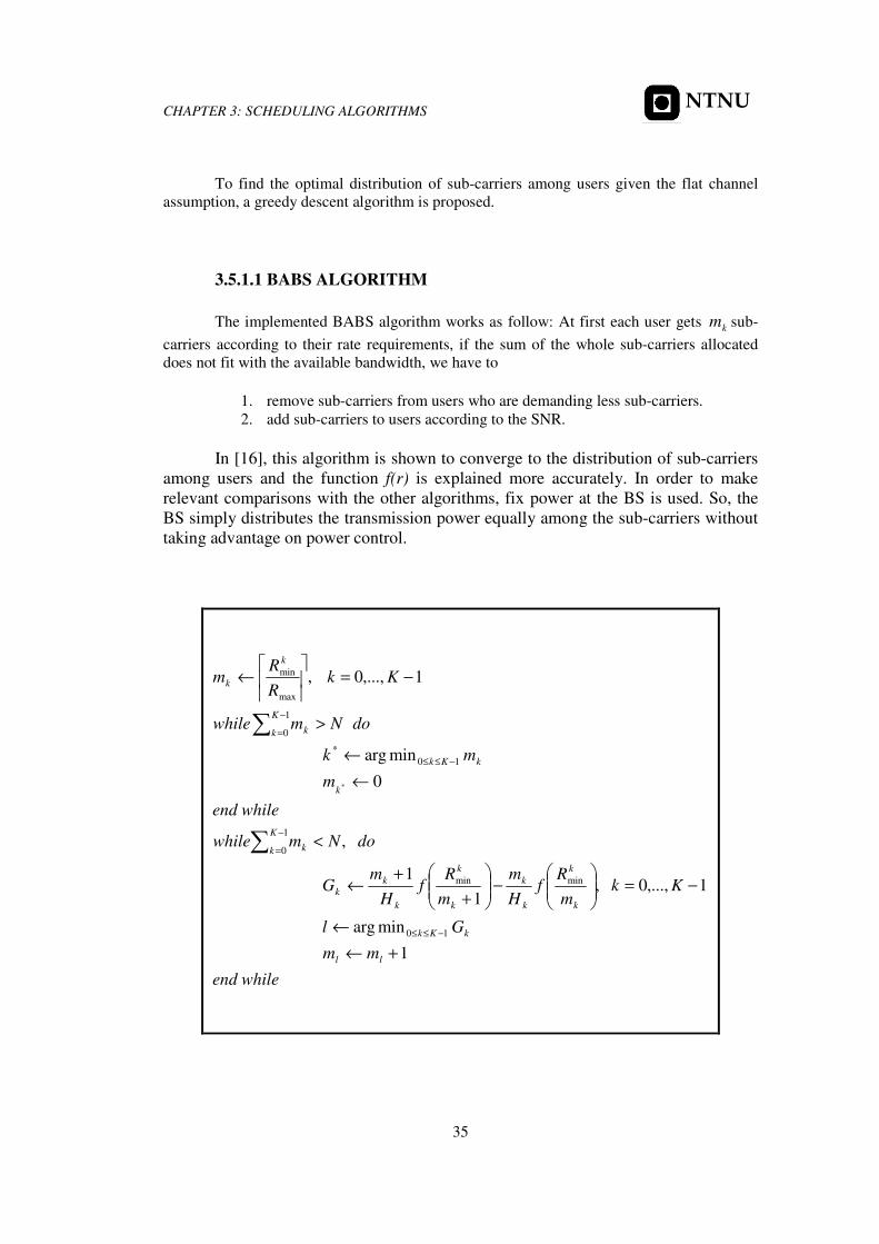
3.4.1 Definition ............................................................................................................................ 30

3.4.2 The Parameter ct ............................................................................................................... 32

3.5 RATE-CRAVING GREEDY ALGORITHM ......................................................................................... 34 3.5.1 BABS................................................................................................................................... 34 3.5.1.1 BABS ALGORITHM ........................................................................................................ 35 3.5.2 RCG .................................................................................................................................... 36 3.5.2.1 RCG ALGORITHM.......................................................................................................... 36 3.5.3 Example Run of the Algorithm............................................................................................ 37

3.6 MATLAB SIMULATIONS ............................................................................................................ 38 3.6.1 Model Description .............................................................................................................. 38 3.6.2 Simulation Results .............................................................................................................. 39 3.6.2.1 Scenario A: Equal Users.................................................................................................. 40 3.6.2.2 Scenario B: Unequal Users ............................................................................................. 42

CHAPTER 4 ........................................................................................................................................ 45

FAIRNESS........................................................................................................................................... 45

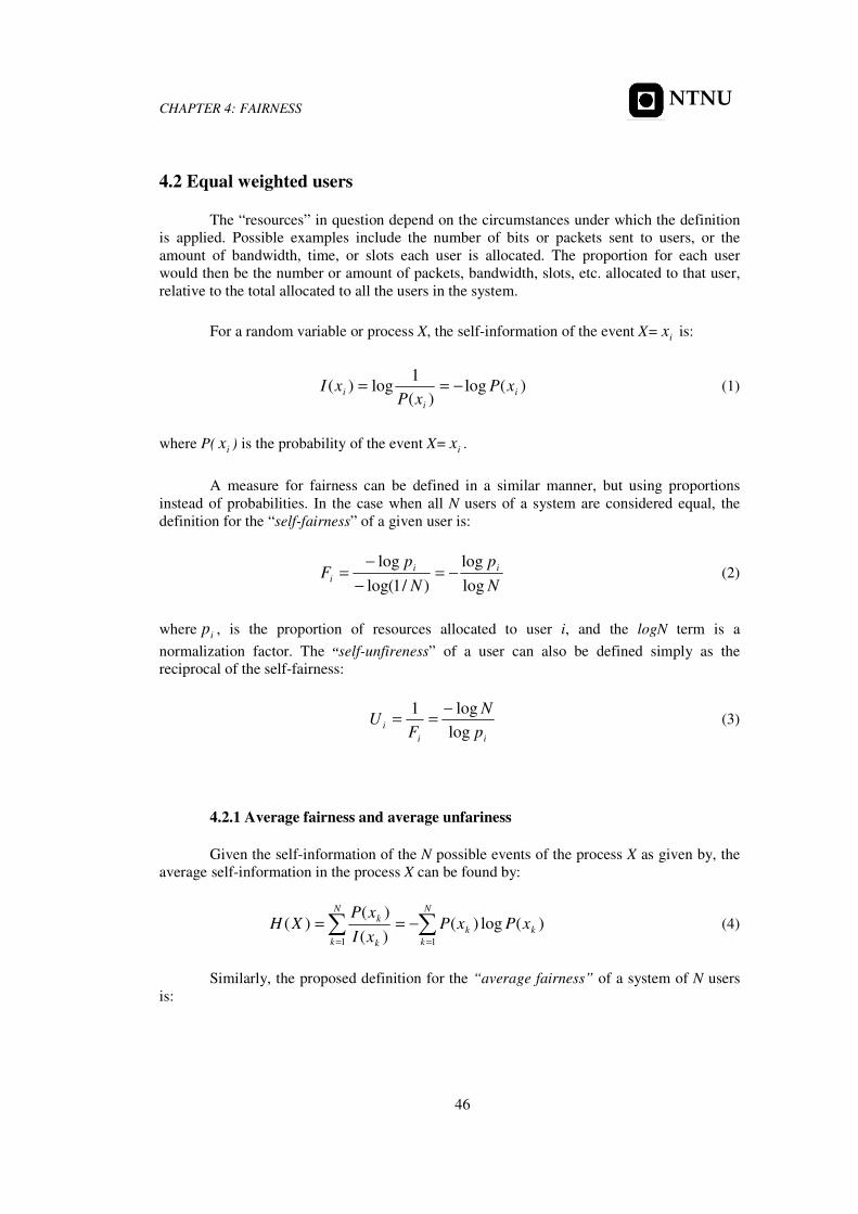
4.1 DEFINITION ................................................................................................................................. 45 4.2 EQUAL WEIGHTED USERS............................................................................................................. 46

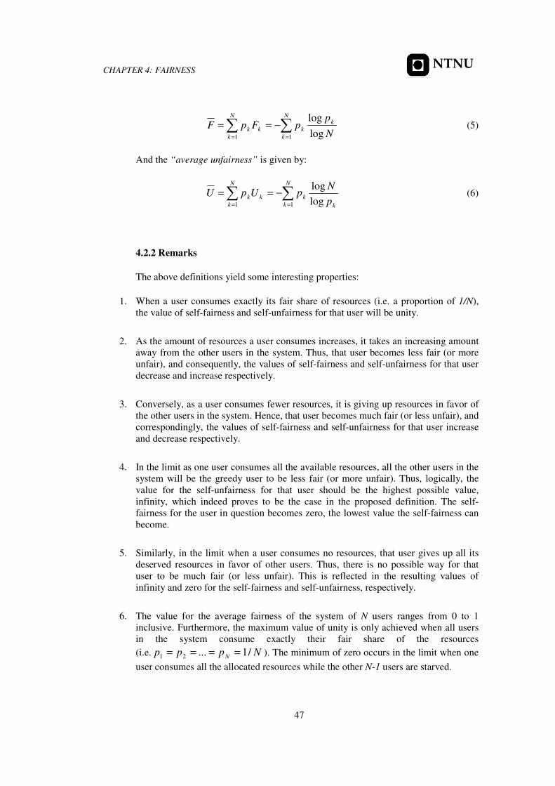
4.2.1 Average fairness and average unfariness ........................................................................... 46 4.2.2 Remarks .............................................................................................................................. 47

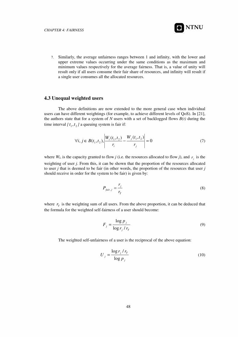
4.3 UNEQUAL WEIGHTED USERS ........................................................................................................ 48 4.3.1 Weighted Average fairness and unfariness......................................................................... 49 4.3.2 Remarks .............................................................................................................................. 49

4.4 MATLAB SIMULATIONS ............................................................................................................ 50 4.4.1 Model Description .............................................................................................................. 50 4.4.2 Simulation Results .............................................................................................................. 50

CHAPTER 5 ........................................................................................................................................ 53

THROUGHPUT.................................................................................................................................. 53

5.1 MOTIVATION ............................................................................................................................... 53 5.2 CHANNEL CAPACITY ................................................................................................................... 53

5.2.1 Shannon-Hartley Theorem.................................................................................................. 54 5.2.2 Outage Capacity ................................................................................................................. 55

5.3 MATLAB SIMULATIONS ............................................................................................................ 55 5.3.1 Model Description .............................................................................................................. 56 5.3.2 Simulation Results .............................................................................................................. 56

CHAPTER 6 ........................................................................................................................................ 59

DELAY................................................................................................................................................. 59

6.1 PREVIOUS WORK.......................................................................................................................... 59 6.2 MATLAB SIMULATIONS ............................................................................................................ 60

6.2.1 Model Description .............................................................................................................. 60 6.2.2 Simulation Results .............................................................................................................. 60

CHAPTER 7 ........................................................................................................................................ 71

CONCLUSIONS ................................................................................................................................. 71

TABLE OF CONTENTS

vi

NTNU

CHAPTER 8 ........................................................................................................................................ 73

FUTURE WORK ................................................................................................................................ 73

APPENDIX A ...................................................................................................................................... 75

A.1 FGN_MODEL.M .......................................................................................................................... 75 A.2 JAKES_MODEL.M ........................................................................................................................ 79

APPENDIX B ...................................................................................................................................... 82

B.1 ALGORITHMS.M........................................................................................................................... 82

APPENDIX C ...................................................................................................................................... 87

C.1 SCHEDULER.M ............................................................................................................................. 87 C.2 STATISTIC.M................................................................................................................................ 89 C.3 THROUGHPUT_FAIRNESS_VS_PFS.M.......................................................................................... 92

APPENDIX D ...................................................................................................................................... 95

D.1 FAIRNESS.M ................................................................................................................................ 95 D.2 THROUGHPUT.M.......................................................................................................................... 98

APPENDIX E ...................................................................................................................................... 99

E.1 THROUGHPUT_FAIRNESS_VS_USERS.M ....................................................................................... 99

APPENDIX F..................................................................................................................................... 101

F.1 PROBABILITY_DELAY.M ............................................................................................................ 101

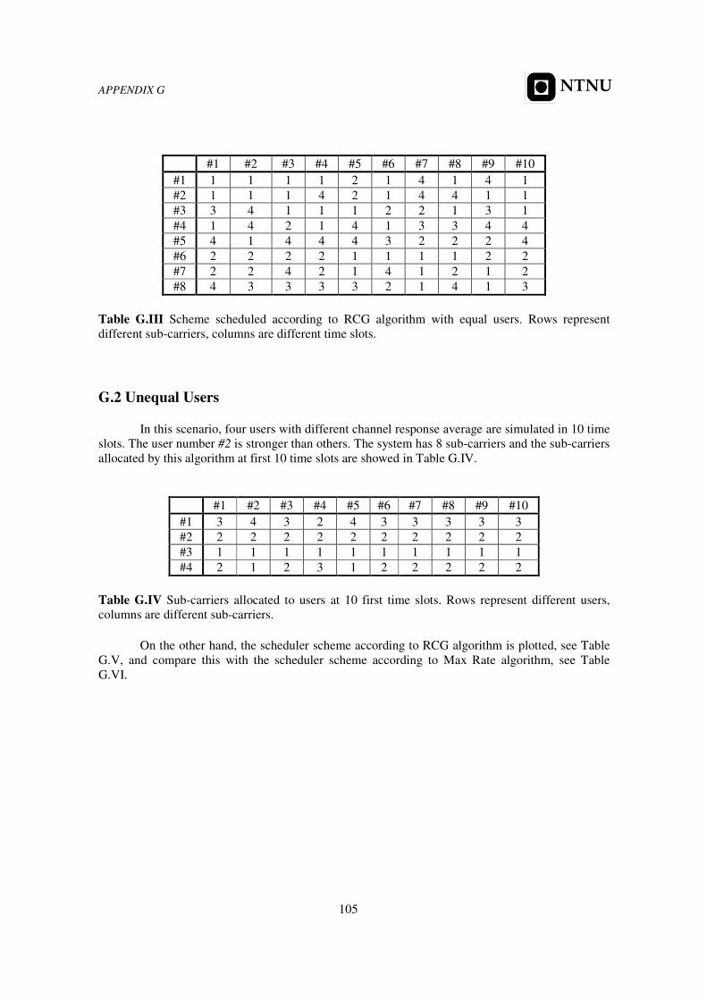
APPENDIX G.................................................................................................................................... 104

G.1 EQUAL USERS........................................................................................................................... 104 G.2 UNEQUAL USERS ...................................................................................................................... 105

REFERENCES.................................................................................................................................. 107

LIST OF TABLES

vii

NTNU

List of Tables

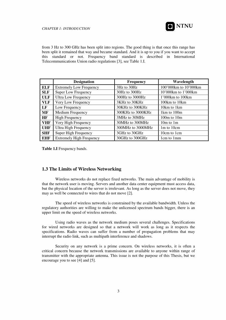
Table 1.I Frequency bands.

Table 3.I Simulation parameters.

Table 3.II (a) Transmission rate demanded by users, (b) sub-carriers demanded by users, (c)

sub-carriers allocated by the algorithm.

Table 3.III Sub-carrier allocation by RCG algorithm at the end of stage 1 (a) and (b) the

algorithm. The number in column k row n is the estimated rate of transmission of user k on

sub-carrier n, if it is allocated that sub-carrier. The blond rate has been chosen.

Table 3.IV Simulation parameters.




Table G.I Transmission rate demanded by users.

Table G.II Sub-carriers allocated to users at 10 first time slots. Rows represent different

users, columns are different sub-carriers.

Table G.III Scheme scheduled according to RCG algorithm with equal users.

Table G.IV Sub-carriers allocated to users at 10 first time slots. Rows represent different

users, columns are different sub-carriers.

Table G.V Scheme scheduled according to RCG algorithm with unequal users. Rows

represent different sub-carriers, columns are different time slots.

Table G.VI Scheme scheduled according to Max Rate algorithm with unequal users.

Rows represent different sub-carriers, columns are different time slots.

LIST OF FIGURES

viii

NTNU

List of Figures

Figure 2.1 Schematic presentation of each component of the multipath signal with two

possible paths.

Figure 2.2 Multipath phenomena, (a) path loss, (b) slow fading, (c) fast fading.

Figure 2.3 Impulse response of the mobile radio channel.

Figure 2.4 Mobile moving along a path segment, while it receives signal from S.

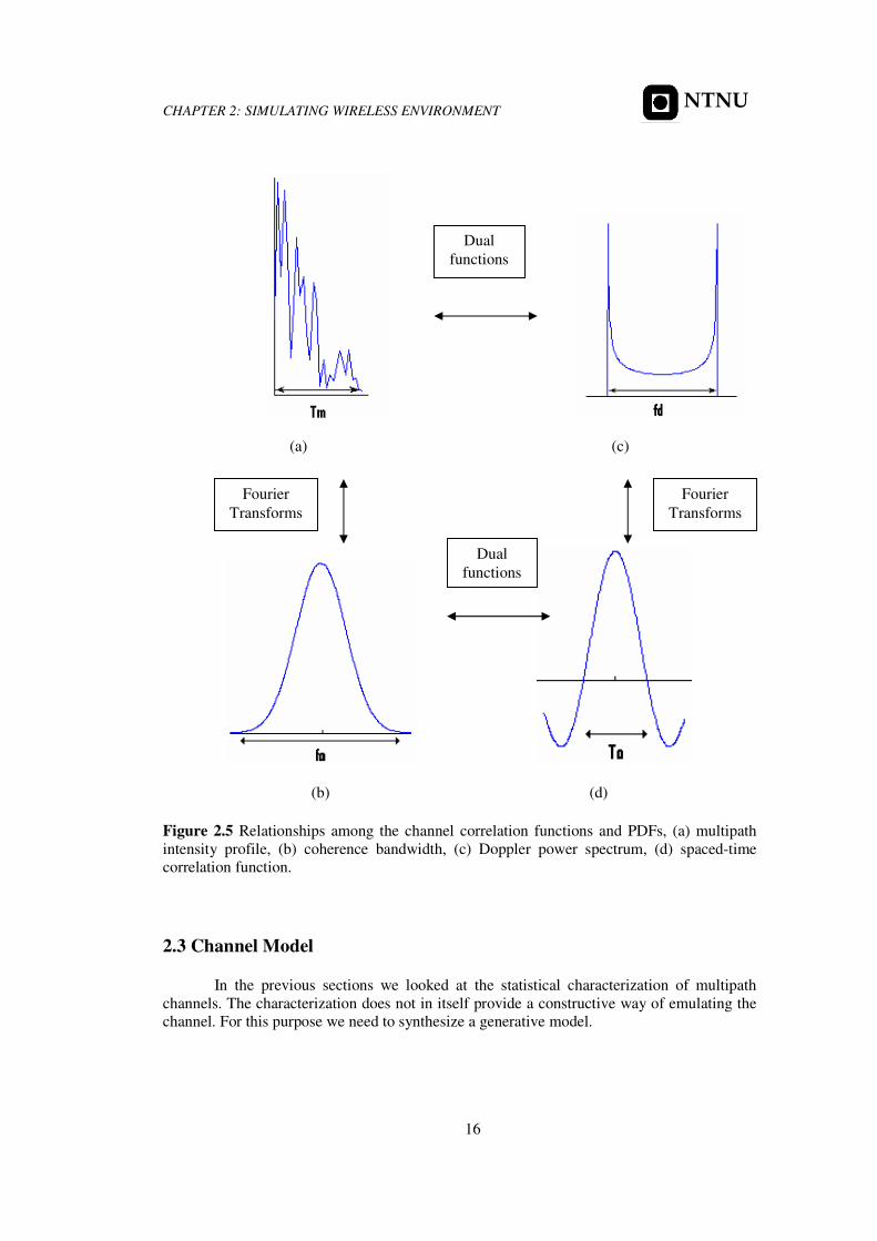
Figure 2.5 Relationships among the channel correlation functions and PDFs, (a) multipath

intensity profile, (b) coherence bandwidth, (c) Doppler power spectrum, (d) spaced-time

correlation function.

Figure 2.6 Tap delay line.

Figure 2.7 Filtered Gaussian Noise model for simulations of a mobile radio channel, (a)

fading envelope, (b) Doppler power spectrum, (c) estimate PDP, (d) frequency channel

response.

Figure 2.8 The Jakes model for simulations of a mobile radio channel when the user is

walking (3km/h), (a) fading envelope, (b) Doppler power spectrum, (c) estimate PDP, (d)

frequency channel response.


driving (80km/h), (a) fading envelope, (b) Doppler power spectrum, (c) estimate PDP, (d)


Figure 2.10 Urban Area where users are walking (3km/h) (a) estimate PDP, (b) frequency

channel response.

Figure 2.11 Hilly Area where users are driving (80km/h) (a) estimate PDP, (b) frequency

channel response.

Figure 2.12 Almost one path (a) estimate PDP, (b) frequency channel response.

Figure 3.1 Multi-carrier transmission system.

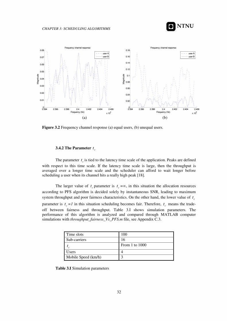
Figure 3.2 Frequency channel response (a) equal users, (b) unequal users.

LIST OF FIGURES

ix

NTNU

Figure 3.3 PFS (dotted line), RR (dotted continuous line) and Max Rate (continuous line)

behaviour versus ct parameter, (a) fairness, (b) throughput.

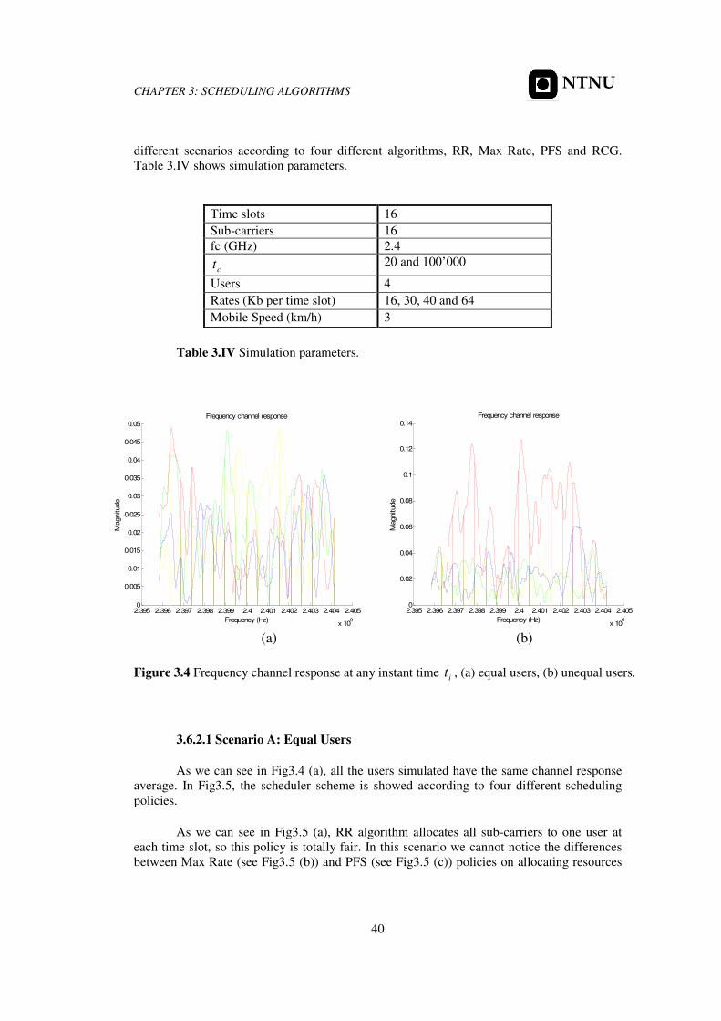
Figure 3.4 Frequency channel response at any instant time it , (a) equal users, (b) unequal

users.

Figure 3.5 Scheme scheduled where users have equal channel responses average and have

been simulated according to filtered Gaussian noise method, (a) RR algorithm, (b) Max Rate

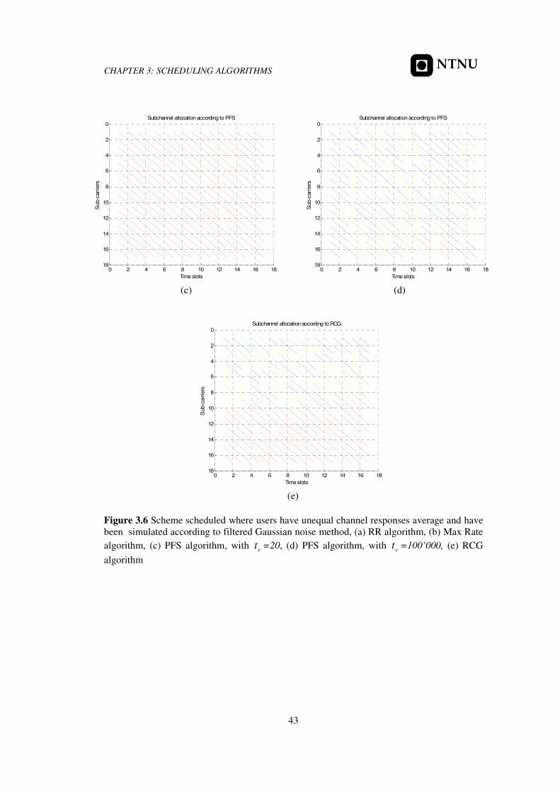
algorithm, (c) PFS algorithm, with ct =20, (d) RCG algorithm.

Figure 3.6 Scheme scheduled where users have unequal channel responses average and have


algorithm, (c) PFS algorithm, with ct =20, (d) PFS algorithm, with

ct =1e5, (e) RCG

algorithm.

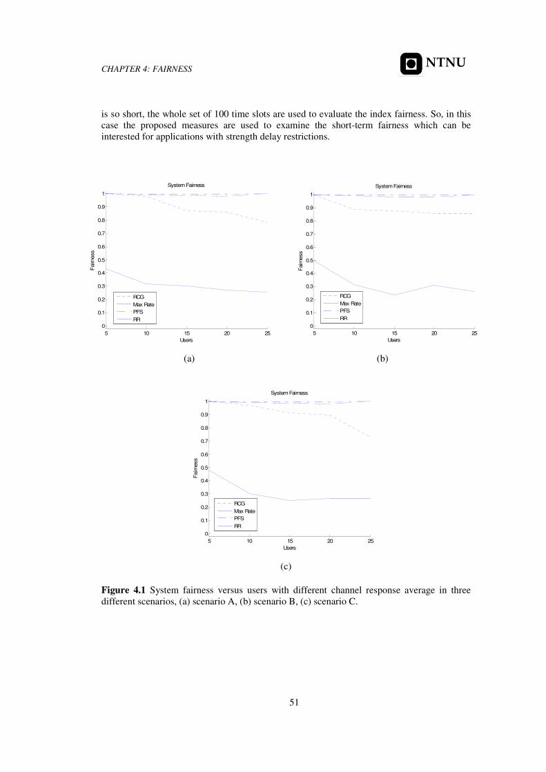
Figure 4.1 System fairness versus users with different channel response average in three

different scenarios, (a) scenario A, (b) scenario B, (c) scenario C.

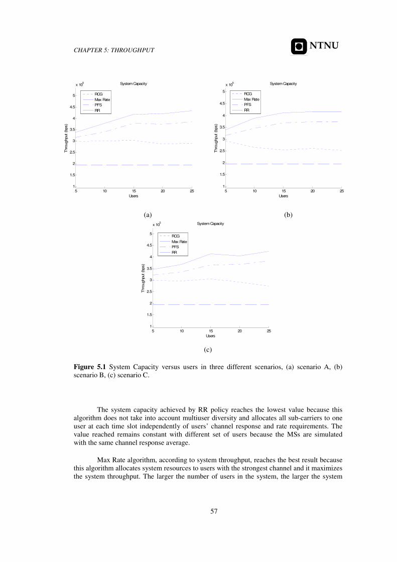
Figure 5.1 System Capacity versus users in three different scenarios, (a) scenario A, (b)

scenario B, (c) scenario C.

Figure 6.1 Probability that a user is transmitting less than Rmin in scenario A with equal

channel response average. (a) 5 users, (b) 10 users, (c) 15 users, (d) 20 users, (e) 25 users.

Figure 6.2 Probability that a user is transmitting less than Rmin in scenario B with equal


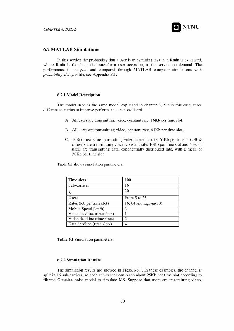
Figure 6.3 Probability that a user is transmitting less than Rmin in scenario C with equal


Figure 6.4 Probability that a user is transmitting less than Rmin in scenario A with unequal


Figure 6.5 Probability that a user is transmitting less than Rmin in scenario B with unequal


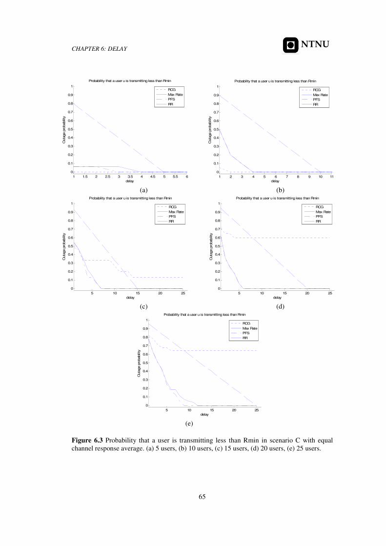
Figure 6.6 Probability that a user is transmitting less than Rmin in scenario C with unequal


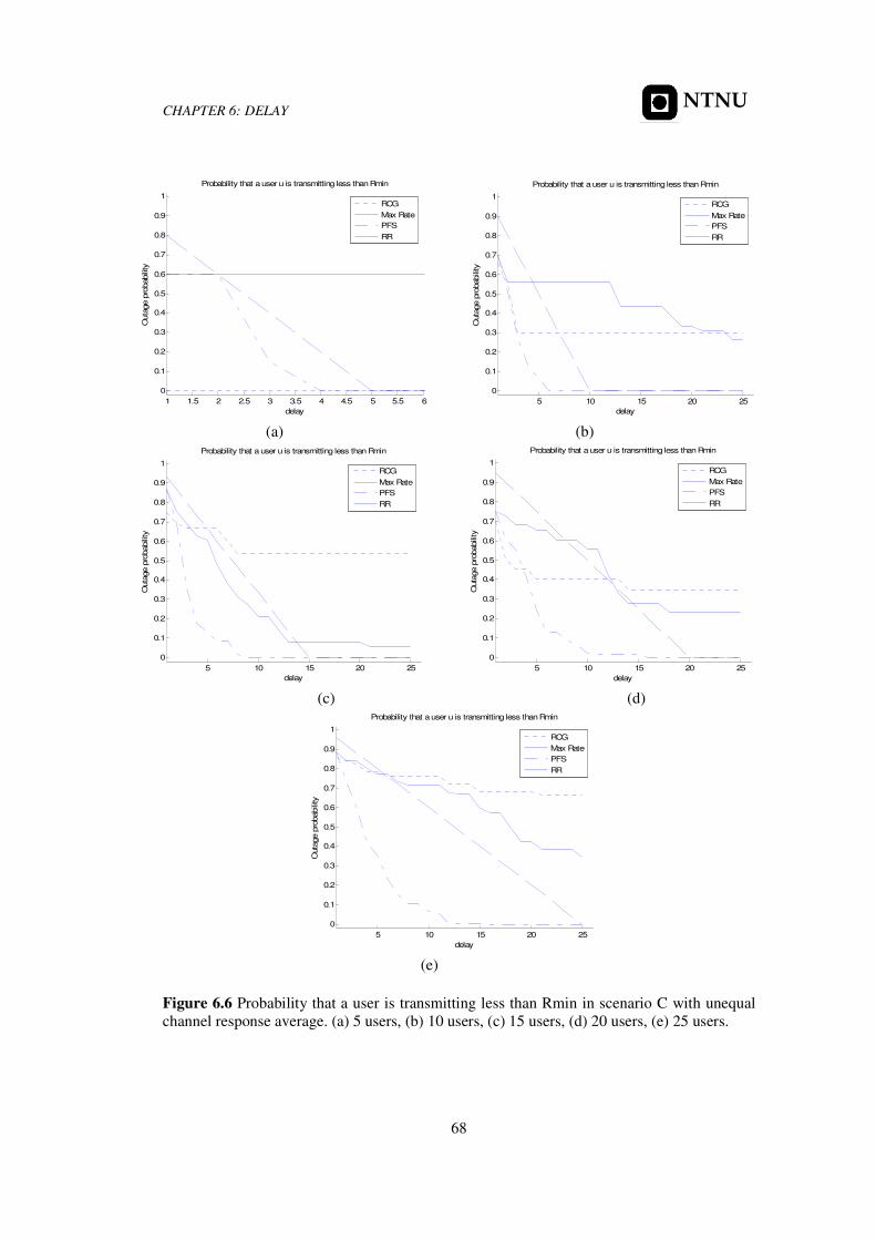
Figure 6.7 Probability that a user is transmitting less than Rmin, with equal channel response

average, (a) scenario A, (b) scenario B, (c) scenario C, with unequal channel response

average (d) scenario A, (e) scenario B, (f) scenario C.

LIST OF ABBREVIATIONS

x

NTNU

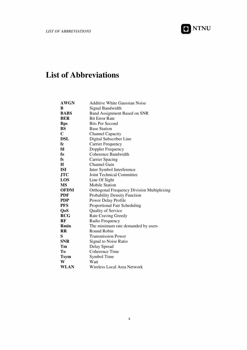
List of Abbreviations

AWGN Additive White Gaussian Noise

B Signal Bandwidth

BABS Band Assignment Based on SNR

BER Bit Error Rate

Bps Bits Per Second

BS Base Station

C Channel Capacity

DSL Digital Subscriber Line

fc Carrier Frequency

fd Doppler Frequency

fo Coherence Bandwidth

fs Carrier Spacing

H Channel Gain

ISI Inter Symbol Interference

JTC Joint Technical Committee

LOS Line Of Sight

MS Mobile Station

OFDM Orthogonal Frequency Division Multiplexing

PDF Probability Density Function

PDP Power Delay Profile

PFS Proportional Fair Scheduling

QoS Quality of Service

RCG Rate Craving Greedy

RF Radio Frequency

Rmin The minimum rate demanded by users

RR Round Robin

S Transmission Power

SNR Signal to Noise Ratio

Tm Delay Spread

To Coherence Time

Tsym Symbol Time

W Watt

WLAN Wireless Local Area Network

CHAPTER 1: INTRODUCTION

1

NTNU

Chapter 1

Introduction

The ability to communicate with people on the move has evolved remarkably since

Guglielmo Marconi first demonstrated radio’s ability to provide continuous contact with

ships sailing the English Channel. That was in 1897, and since then new wireless

communications methods and services has been enthusiastically adopted by people

throughout the world. Particularly during the past ten years, the mobile wireless

communications industry has grown by orders of magnitude, fueled by digital and RF circuit

fabrication improvements, new large-scale circuit integration, and other miniaturization

technologies which make portable radio equipment smaller, cheaper, and more reliable [1].

The most successful wireless networking technology this far has been 802.11.

Orthogonal frequency division multiplexing (OFDM) has become a popular

technique for transmission of signals over wireless channels. OFDM has been adopted in

several wireless standards like 802.11. OFDM converts a frequency-selective channel into a

parallel collection of frequency flat sub-channels. The sub-carriers have the minimum

frequency separation required to maintain orthogonality of their corresponding time domain

waveforms, yet the signal spectra corresponding to the different sub-carriers overlap in

frequency. Hence, the available bandwidth is used very efficiently. If knowledge of the

channel is available at the transmitter, then the OFDM transmitter can adapt its signalling

strategy to match the channel.

OFDM devices use one wide frequency channel by breaking it up into several

components sub-carriers. Each sub-carrier is used to transmit data. All the “slow” sub-

carriers are then multiplexed into one “fast” combine channel.

OFDM is not a new technique. Most of the fundamental work was done in the late

1960s. Recent DSL work and wireless data applications have rekindled interest in OFDM,

especially now that better signal-processing techniques make it more practical [2].


2

NTNU

1.1 Motivation

Wireless networks offer several advantages over fixed (or “wired”) networks:

Mobility

Users move, but data is usually stored centrally. Enabling users to access

data while they are in motion can lead to large productivity gains.

Ease and speed of deployment

Many areas are difficult to wire for traditional mired LANs. Older buildings

are often a problem; running cable through the walls of an older stone

building to which the blueprints have been lost can be a challenge. In many

places, historic preservation laws make it difficult to carry out new LAN

installation in older buildings.

Flexibility

No cables mean no recabling. Wireless networks allow users to quickly form

amorphous, small group networks for meeting, and wireless networking

makes moving between cubicles and office a snap. Expansion with wireless

networks is easy because the network medium is already everywhere. There

are no cables to pull, connect, or trip over.

Cost

In some cases, costs can be reduced by using wireless technology. As an

example, 802.11 equipment can be used to create a wireless bridge between

two buildings. Setting up a wireless bridge requires some initial capital cost

in terms of outdoor equipment, access points and wireless interfaces. After

the initial capital expenditure, however, an 802.11-based, LOS network will

have only a negligible recurring monthly operating cost. Over time, point-to-

point wireless links are far cheaper than leasing capacity from the telephone

company.

1.2 Radio Spectrum: The Key Resource

Wireless devices are constrained to operate in a certain frequency band. Each band

has an associated bandwidth, which is simply the amount of frequency space in the band.

Bandwidth has acquired a connotation of being a measure of the data capacity of a link [22].

A great deal of mathematics, information theory and signal processing can be used to show

that higher-bandwidth slices can be used to transmit more information. The use of a radio

spectrum is rigorously controlled by regulatory authorities through licensing processes. Each

frequency range has a band designator and each range of frequencies behaves differently and

performs different functions. The frequency spectrum is shared by civil, government, and

military users of all nations according to International Telecommunications Union (ITU)

radio regulations. For communications purposes, the usable frequency spectrum now extends

from about 3 Hz to about 300 GHz. There are also some experiments at about 100 THz where

research on laser communications is taking place but we won't discuss this now. This range


3

NTNU

from 3 Hz to 300 GHz has been split into regions. The good thing is that once this range has

been split it remained that way and became standard. And it is up to you if you want to accept

this standard or not. Frequency band standard is described in International

Telecommunications Union radio regulations [3], see Table 1.I.

Designation Frequency Wavelength

ELF Extremely Low Frequency 3Hz to 30Hz 100’000km to 10’000km

SLF Super Low Frequency 30Hz to 300Hz 10’000km to 1’000km

ULF Ultra Low Frequency 300Hz to 3000Hz 1’000km to 100km

VLF Very Low Frequency 3KHz to 30KHz 100km to 10km

LF Low Frequency 30KHz to 300KHz 10km to 1km

MF Medium Frequency 300KHz to 3000KHz 1km to 100m

HF High Frequency 3MHz to 30MHz 100m to 10m

VHF Very High Frequency 30MHz to 300MHz 10m to 1m

UHF Ultra High Frequency 300MHz to 3000MHz 1m to 10cm

SHF Super High Frequency 3GHz to 30GHz 10cm to 1cm

EHF Extremely High Frequency 30GHz to 300GHz 1cm to 1mm

Table 1.I Frequency bands.

1.3 The Limits of Wireless Networking

Wireless networks do not replace fixed networks. The main advantage of mobility is

that the network user is moving. Servers and another data center equipment must access data,

but the physical location of the server is irrelevant. As long as the server does not move, they

may as well be connected to wires that do not move [2].

The speed of wireless networks is constrained by the available bandwidth. Unless the

regulatory authorities are willing to make the unlicensed spectrum bands bigger, there is an

upper limit on the speed of wireless networks.

Using radio waves as the network medium poses several challenges. Specifications

for wired networks are designed so that a network will work as long as it respects the

specifications. Radio waves can suffer from a number of propagation problems that may

interrupt the radio link, such as multipath interference and shadows.

Security on any network is a prime concern. On wireless networks, it is often a

critical concern because the network transmissions are available to anyone within range of

transmitter with the appropriate antenna. This issue is not the purpose of this Thesis, but we

encourage you to see [4] and [5].


4

NTNU

1.4 Objectives

The subject to deal with is simulating a wireless communication between a BS and

multiple MSs where radio link is shared. The Thesis results in a MATLAB simulator for the

radio channel in a system with a fixed BS and moving user terminals (MSs). The simulations

are based on a simplistic geometrical model for the radio environment.

In this project, the tool to be used for simulating is MATLAB 7.0.019920 (R14).

With this tool we have to achieve the following two objectives the most important in the

Master Thesis:

� Simulating radio link between two terminals.

� Evaluating different scheduling policies for allocating resources according to

three properties, fairness, throughput and delay.

Other “collateral” objectives are:

o Getting knowledge about wireless communications.

o Getting to understand mathematical artifacts commonly implemented for

simulating radio channels.

o Practising programming skills, which will be applied in MATLB scripts.

o Promoting the student’s skills for making decisions and choosing creative

solutions design which will be applied in the final solution and in the

definition of a set of experiments to prove performance.

1.5 Report structure

The current paper is organized in eight chapters and seven appendices.

In Chapter 2, a general idea of channel characterization and modeling are presented.

And the main underlying theoretical concepts about channel modeling are given.

In Chapter 3, a general idea of multiuser diversity is showed. In order to improve the

throughput of multiple packet-data users sharing a wireless channel while preserving fairness,

different scheduling algorithms in different scenarios are proposed.

In Chapter 4, fairness which is one of the most important properties in a wireless

environment where system resources are sharing is introduced and discussed. And the

different behaviour from different scheduling policies on index fairness is showed.

In Chapter 5, throughput which is one of the most important properties of an

information system is introduced and discussed. In this chapter the different behaviour from

different scheduling policies is evaluated in different scenarios.


5

NTNU

In Chapter 6, delay which is one of the most important properties of current

applications is introduced and discussed. In this chapter the delay of different applications

(video, voice and data) is evaluated in different scenarios and with different scheme

scheduling to achieve QoS.

Chapter 7 from the main ideas presented throughout the text, the main conclusions

are extracted.

Chapter 8 points out possible future works to extend this Thesis.

Appendices are devoted to show the MATLAB scripts which have been used for

simulating the theoretical concepts.

In Appendix A, the scripts to simulate the radio channel behaviour are showed

according to two different approximations, filtered Gaussian noise process and Jakes model.

In Appendix B, the algorithms which are used by the scheduler in the BS are showed,

these are Max Rate, RR, PFS and RCG.

In Appendix C, are showed the scripts which simulate the BS scheduler, the statistics

resulted from the scheduler scheme and the script used to evaluate PFS behaviour with

different ct parameter values.

In Appendix D, the scripts which compute the index fairness and system throughput

are showed.

In Appendix E, the script which computes the index fairness and system throughput

versus users is showed.

In Appendix F, the script which computes the probability that a user is transmitting

less than the demanded rate is showed.


6

NTNU

CHAPTER 2: SIMULATING WIRELESS ENVIRONMENT

7

NTNU

Chapter 2

Channel Modeling

Understanding the behavior of the wireless medium is essential for appreciating the

reasoning behind specific designs for wireless communications protocols. In particular,

physical-layer and medium-access protocol designs are influenced heavily by the behavior of

the channel, which varies substantially in different locations.

The effective design, assessment, and installation of a radio network require accurate

characterization of the channel. The channel characteristics vary from one environment to

another, and the particular characteristics determine the feasibility of using a proposed

communication technique in a given operation environment. Having an accurate channel

characterization for each frequency band and a detailed mathematical model of the channel,

enables the designer or user of a wireless system to predict signal coverage, achievable data

rate, and the specific performance attributes of alternative signaling and reception schemes.

The wireless network that we consider in this Thesis operates at frequency of 2.4

GHz according to IEEE 802.11- based WLANs. Frequencies in the region of few gigahertz

have several attractive features for being used in wireless information networks. At these

frequencies a transmitter with power of less than 1 W can provide coverage distances on the

order of a few miles, as needed for cellular urban radio communications. Furthermore, at

these frequencies the size of an efficient antenna can be on the order of an inch, and antenna

separation as small as several inches can provide uncorrelated received signals suitable for

achieving diversity in the received signal [6].

2.1 Fading and Multipath Channels

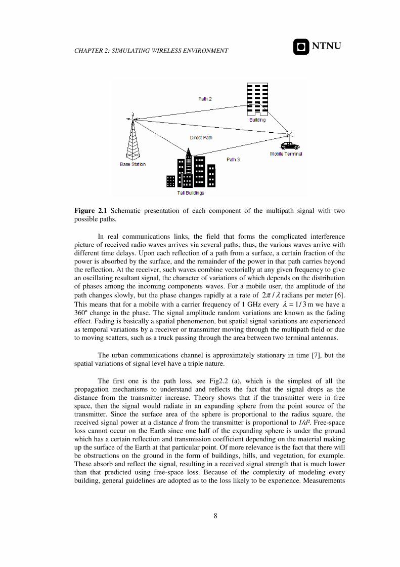
Most cellular wireless systems operate in built-up areas where there is no direct LOS

radio path between the terminals, the transmitter and the receiver and where, due to natural

and man-made obstructions (hill, trees, buildings, towers…), multidiffraction,

multireflection, and multiscattering effects occurs (see Fig2.1). These cause not only

additional losses (with respect to those obtained in LOS above the terrain), but also multipath

fading of the signal strength observed at the receiver [9].


8

NTNU

Figure 2.1 Schematic presentation of each component of the multipath signal with two

possible paths.

In real communications links, the field that forms the complicated interference

picture of received radio waves arrives via several paths; thus, the various waves arrive with

different time delays. Upon each reflection of a path from a surface, a certain fraction of the

power is absorbed by the surface, and the remainder of the power in that path carries beyond

the reflection. At the receiver, such waves combine vectorially at any given frequency to give

an oscillating resultant signal, the character of variations of which depends on the distribution

of phases among the incoming components waves. For a mobile user, the amplitude of the

path changes slowly, but the phase changes rapidly at a rate of λπ /2 radians per meter [6].

This means that for a mobile with a carrier frequency of 1 GHz every 3/1=λ m we have a

360º change in the phase. The signal amplitude random variations are known as the fading

effect. Fading is basically a spatial phenomenon, but spatial signal variations are experienced

as temporal variations by a receiver or transmitter moving through the multipath field or due

to moving scatters, such as a truck passing through the area between two terminal antennas.

The urban communications channel is approximately stationary in time [7], but the

spatial variations of signal level have a triple nature.

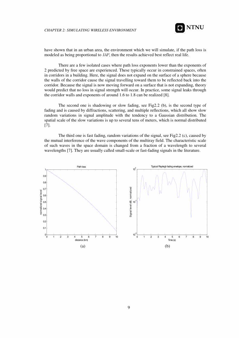
The first one is the path loss, see Fig2.2 (a), which is the simplest of all the

propagation mechanisms to understand and reflects the fact that the signal drops as the

distance from the transmitter increase. Theory shows that if the transmitter were in free

space, then the signal would radiate in an expanding sphere from the point source of the

transmitter. Since the surface area of the sphere is proportional to the radius square, the

received signal power at a distance d from the transmitter is proportional to 1/d². Free-space

loss cannot occur on the Earth since one half of the expanding sphere is under the ground

which has a certain reflection and transmission coefficient depending on the material making

up the surface of the Earth at that particular point. Of more relevance is the fact that there will

be obstructions on the ground in the form of buildings, hills, and vegetation, for example.

These absorb and reflect the signal, resulting in a received signal strength that is much lower

than that predicted using free-space loss. Because of the complexity of modeling every

building, general guidelines are adopted as to the loss likely to be experience. Measurements


9

NTNU

have shown that in an urban area, the environment which we will simulate, if the path loss is

modeled as being proportional to 1/d³, then the results achieved best reflect real life.

There are a few isolated cases where path loss exponents lower than the exponents of

2 predicted by free space are experienced. These typically occur in constrained spaces, often

in corridors in a building. Here, the signal does not expand on the surface of a sphere because

the walls of the corridor cause the signal travelling toward them to be reflected back into the

corridor. Because the signal is now moving forward on a surface that is not expanding, theory

would predict that no loss in signal strength will occur. In practice, some signal leaks through

the corridor walls and exponents of around 1.6 to 1.8 can be realized [8].

The second one is shadowing or slow fading, see Fig2.2 (b), is the second type of

fading and is caused by diffractions, scattering, and multiple reflections, which all show slow

random variations in signal amplitude with the tendency to a Gaussian distribution. The

spatial scale of the slow variations is up to several tens of meters, which is normal distributed

[7].

The third one is fast fading, random variations of the signal, see Fig2.2 (c), caused by

the mutual interference of the wave components of the multiray field. The characteristic scale

of such waves in the space domain is changed from a fraction of a wavelength to several

wavelengths [7]. They are usually called small-scale or fast-fading signals in the literature.

0 1 2 3 4 5 6 7 8 9 100

0.1

0.2

0.3

0.4

0.5

0.6

0.7

0.8

0.9

1Path loss

distance (km)

norm

aliz

ed s

ignal le

vel

0 1 2 3 4 5 6 7 8 9 1010

-2

10-1

100

Typical Rayleigh fading envelope, normalized

Time (s)

Sig

nal le

vel dB

, norm

aliz

ed

(a) (b)


10

NTNU

0 1 2 3 4 5 6 7 8 9 1010

-2

10-1

100


Time (s)

Sig

nal le

vel dB

, norm

aliz

ed

(c)

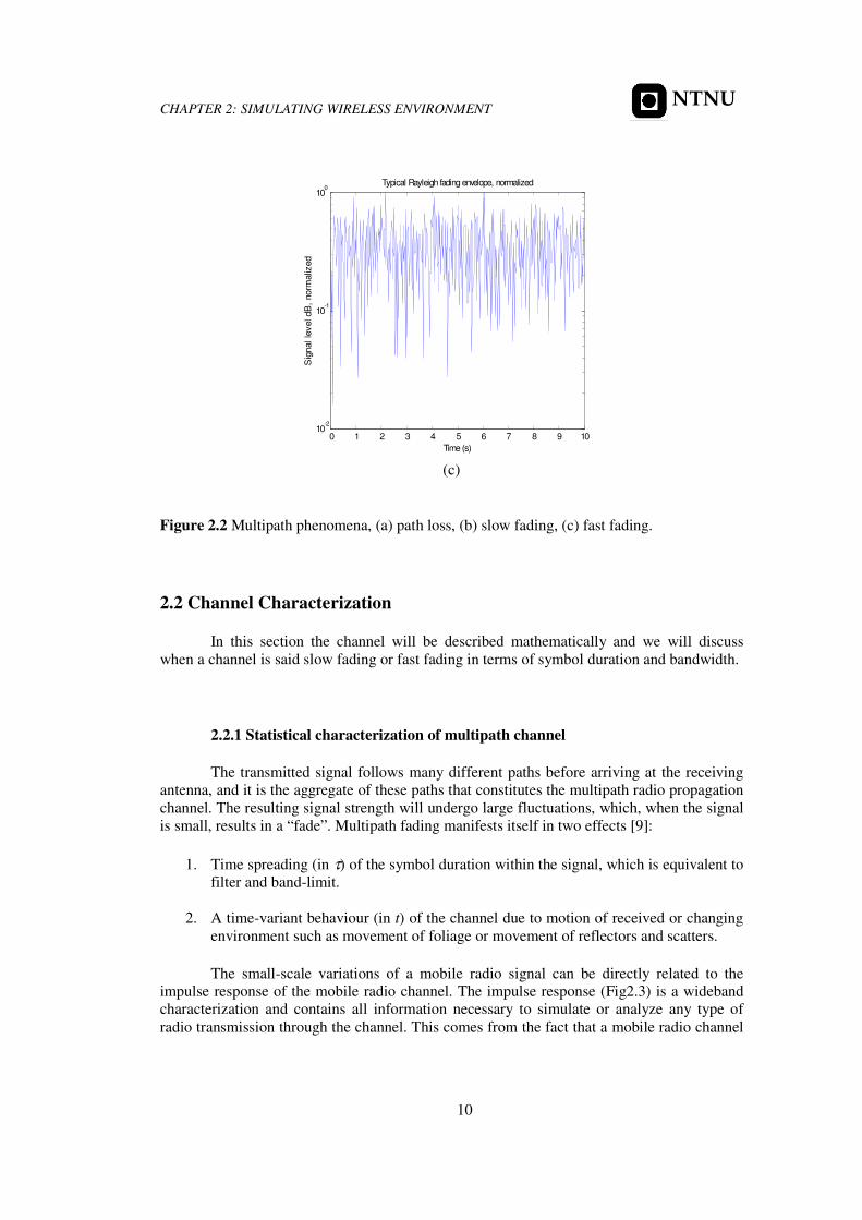
Figure 2.2 Multipath phenomena, (a) path loss, (b) slow fading, (c) fast fading.

2.2 Channel Characterization

In this section the channel will be described mathematically and we will discuss

when a channel is said slow fading or fast fading in terms of symbol duration and bandwidth.

2.2.1 Statistical characterization of multipath channel

The transmitted signal follows many different paths before arriving at the receiving

antenna, and it is the aggregate of these paths that constitutes the multipath radio propagation

channel. The resulting signal strength will undergo large fluctuations, which, when the signal

is small, results in a “fade”. Multipath fading manifests itself in two effects [9]:

1. Time spreading (in τ) of the symbol duration within the signal, which is equivalent to

filter and band-limit.

2. A time-variant behaviour (in t) of the channel due to motion of received or changing

environment such as movement of foliage or movement of reflectors and scatters.

The small-scale variations of a mobile radio signal can be directly related to the

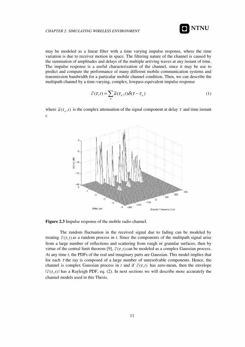
impulse response of the mobile radio channel. The impulse response (Fig2.3) is a wideband

characterization and contains all information necessary to simulate or analyze any type of

radio transmission through the channel. This comes from the fact that a mobile radio channel


11

NTNU

may be modeled as a linear filter with a time varying impulse response, where the time

variation is due to receiver motion in space. The filtering nature of the channel is caused by

the summation of amplitudes and delays of the multiple arriving waves at any instant of time.

The impulse response is a useful characterization of the channel, since it may be use to

predict and compare the performance of many different mobile communication systems and

transmission bandwidth for a particular mobile channel condition. Then, we can describe the

multipath channel by a time-varying, complex, lowpass-equivalent impulse response

∑ −=n

nn tatc )(),(~),(~ ττδττ (1)

where ),(~ ta nτ is the complex attenuation of the signal component at delay τ and time instant

t.

Figure 2.3 Impulse response of the mobile radio channel.

The random fluctuation in the received signal due to fading can be modeled by

treating ),(~ tc τ as a random process in t. Since the components of the multipath signal arise

from a large number of reflections and scattering from rough or granular surfaces, then by

virtue of the central limit theorem [9], ),(~ tc τ can be modeled as a complex Gaussian process.

At any time t, the PDFs of the real and imaginary parts are Gaussian. This model implies that

for each τ the ray is composed of a large number of unresolvable components. Hence, the

channel is complex Gaussian process in t and if ),(~ tc τ has zero-mean, then the envelope

| ),(~ tc τ | has a Rayleigh PDF, eq. (2). In next sections we will describe more accurately the

channel models used in this Thesis.


12

NTNU

)2/(

2

22

)( σ

σr

R er

rf−= (2)

2.2.2 The Power Delay Profile

An example of the power delay profile (PDP) is showed in Fig2.5 (a). Here, the term

delay, refers to excess delay. It represents the delay measured from the first perceptible signal

that arrives at the receiver. The maximum excess delay, also termed maximum delay spread,

mT is the delay between the first and the last component of the signal during which the

received power fall below some threshold level, e.g. 20 dB below the strongest component.

The relationship between mT and the symbol time symT can be viewed in terms of two

different degradation criteria [9]:

1. A channel is said to exhibit frequency-selective fading if mT > symT . In this condition,

the multipath components extend beyond the symbol duration, which causes ISI

distorsion in the signal. Since the multipath is resolvable in this case, the ISI

distortion can be mitigated by rake reception or equalization.

2. A channel is said to exhibit frequency-nonselective or flat fading if mT < symT . In this

case there is very little ISI, but we still have distortion in the system because the

multipath signal can add destructively, reducing the SNR considerably.

The dividing line between frequency-selective and flat fading is not perfectly sharp.

In channels that we call flat, frequency selective still happens, but with smaller probability.

2.2.3 The Spaced-Frequency Correlation Function

As we can see in Fig2.5 (b), a completely analogous characterization of signal

dispersion can be done in the frequency domain. The function is defined as the Fourier

transform of the PDP. Spaced-frequency correlation function represents the correlation

between the channel response to two narrowband signals with the frequencies 1f and 2f as a

function of the difference 12 fff −=∆ . This function can be thought of as the transfer of the

channel. Therefore, time spreading can be viewed as if it was the result of a filtering process.

The coherence bandwidth0f is defined as the frequency range where all frequency

component amplitudes are correlated. That is, the spectral components in that range fade

together. It can be shown that 0f and mT are reciprocally related. As a rule of thumb, it is

usually assumed that


13

NTNU

mTf

10 ≈ (3)

For the case of the mobile radio, an array of radially uniformly spaced scatters, all

with equal-magnitude reflection coefficients, but independent, randomly occurring phase

angles, is widely accepted. This model is referred as the dense scatter channel model, and is

commonly known as the Jakes model which will be described in section 2.3.2.

The two degradation criteria above for frequency-selective and flat fading can also be

expressed in terms of the coherence and signal bandwidths:

1. A channel is referred as frequency-selective if 0f < B, where B is the signal

bandwidth. Since the channel coherence bandwidth is smaller than the signal

bandwidth, the channel acts as a filter, hence frequency-selective fading occurs.

2. Frequency-nonselective or flat fading degradation occurs whenever 0f >> B. As

noted before, flat fading does not introduce ISI, but performance degradation occurs

due to low SNR whenever the signal is fading. It should be noted that frequency

selectivity diminishes as 0f /B is increasingly larger than 1.

Flat fading is not always desirable. For example, to achieve frequency diversity for

two fading signals, it is necessary that the carrier spacing sf between the two signals is

larger than the coherence bandwidth, sf > 0f , so that the two signals are uncorrelated [9].

2.2.4 The Time-Varying Channel

In this and the next section will be described the properties of the channel as they

relate to its time-varying nature. For mobile radio applications, the channel is time-varying

because the motion between the transmitter and the receiver results in propagation path

changes. It should be noted that since the channel characteristics are dependent on the relative

position of the transmitter and receiver, time variance is equivalent to space variance. The

time variation of the channel is characterized by the Doppler power spectrum S(υ), shown in

Fig2.5 (c).

2

max

max

1( )

1d

d

S

ff

ν

νπ

=

−

maxdf≤ν (4)

where as it will be seen in section 2.2.4.2, maxdf is the maximum Doppler frequency shift.


14

NTNU

2.2.4.1 The Spaced-Time Correlation Function

The spaced-time correlation function ρ(∆t), Fig2.5 (d) is the inverse Fourier

transform of S(υ), and it specifies the correlation between the channel’s response to a

narrowband signal sent at times 1t and 2t , where 12 ttt −=∆ . The coherence time, 0T , is the

expected time duration within the two signals remain correlated. If the channel is time-

invariant, 1)( =∆tρ . Coherence time can also be measured in distance traversed [9].

The time-variant behaviour is categorized into fast fading and slow fading:

1. A channel is said to be fast fading if 0T < symT , where 0T is the channel coherence

time and symT is the symbol time. During the fast fading the baseband symbol shapes

can be severely distorted, which often results in an irreducible BER and

synchronization problems.

2. A channel is referred as slow fading if 0T > symT . The time duration that the channel

remains correlated is long compared to the transmitted symbol. The primary in a

slow fading channel is the loss of SNR.

2.2.4.2 Doppler Power Spectrum

The Doppler power spectrum has been shown to match experimental data gathered

for outdoor mobile radio channels. For indoor mobile radio channels a flat spectrum is used

[9].

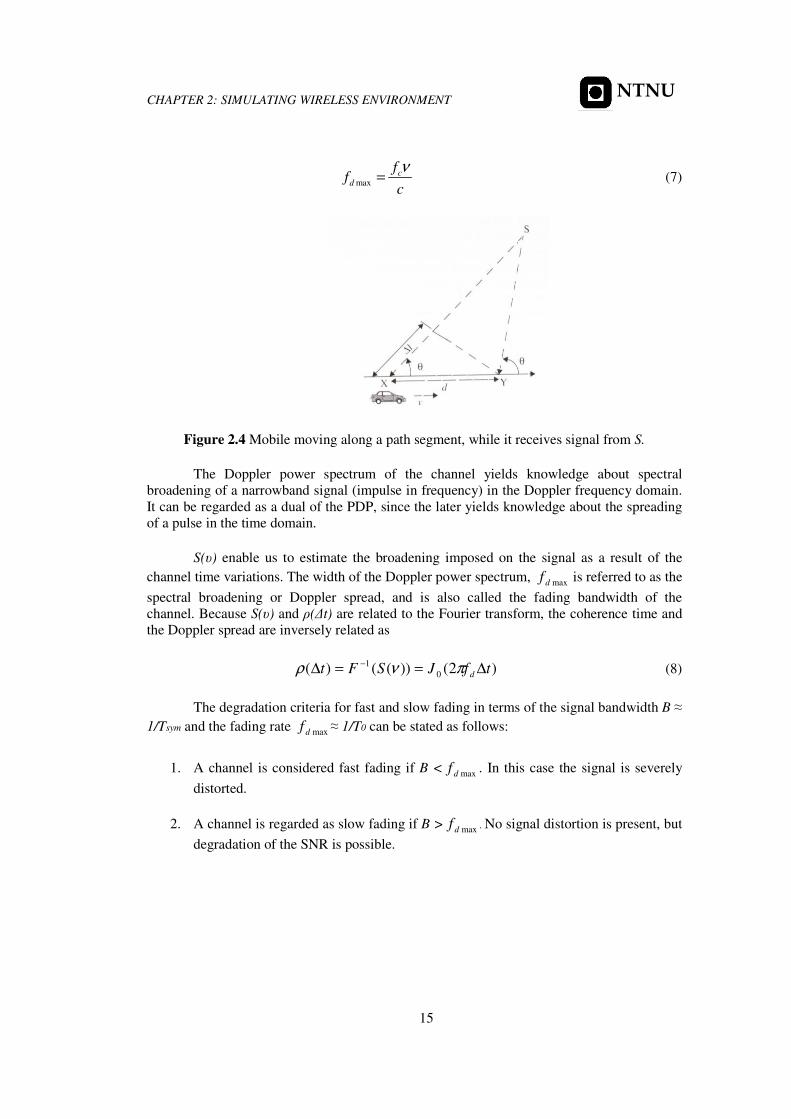
Consider a mobile moving a constant velocity v, along a path segment having length

d between points X and Y, while it receives signals from a remote source S, as illustrated in

Fig2.4. The differences in path lengths travelled by the wave from source S to the mobile at

points X and Y is ∆l = dcosθ = v∆tcosθ, where ∆t is the time required for the mobile to travel

from X to Y, and θ is assumed to be the same at points X and Y since the source is assumed to

be very far away. The phase change in the received signal due to the difference in path

lengths is therefore

θλ

πν

λ

πϕ cos

22 tl ∆=

∆=∆ (5)

and hence the apparent change in frequency, or Doppler shift, is given by df , where

coscd

ff

c

νθ= (6)

the maximum Doppler frequency is


15

NTNU

maxc

d

ff

c

ν= (7)

Figure 2.4 Mobile moving along a path segment, while it receives signal from S.

The Doppler power spectrum of the channel yields knowledge about spectral

broadening of a narrowband signal (impulse in frequency) in the Doppler frequency domain.

It can be regarded as a dual of the PDP, since the later yields knowledge about the spreading

of a pulse in the time domain.

S(υ) enable us to estimate the broadening imposed on the signal as a result of the

channel time variations. The width of the Doppler power spectrum, maxdf is referred to as the

spectral broadening or Doppler spread, and is also called the fading bandwidth of the

channel. Because S(υ) and ρ(∆t) are related to the Fourier transform, the coherence time and

the Doppler spread are inversely related as

)2())(()( 0

1 tfJSFt d ∆==∆ − πνρ (8)

The degradation criteria for fast and slow fading in terms of the signal bandwidth B ≈

1/Tsym and the fading rate maxdf ≈ 1/T0 can be stated as follows:

1. A channel is considered fast fading if B <maxdf . In this case the signal is severely

distorted.

2. A channel is regarded as slow fading if B > maxdf . No signal distortion is present, but

degradation of the SNR is possible.


16

NTNU

(a) (c)

(b) (d)

Figure 2.5 Relationships among the channel correlation functions and PDFs, (a) multipath

intensity profile, (b) coherence bandwidth, (c) Doppler power spectrum, (d) spaced-time

correlation function.

2.3 Channel Model

In the previous sections we looked at the statistical characterization of multipath

channels. The characterization does not in itself provide a constructive way of emulating the

channel. For this purpose we need to synthesize a generative model.

Dual

functions

Dual

functions

Fourier

Transforms

Fourier

Transforms


17

NTNU

Simulation of envelope fading is very important for design and performance

evaluation of wireless modems because often we cannot find closed-form solutions to

compare performance of various modulation and coding techniques over wireless channels.

To simulate a narrowband channel, we need to generate a random process with a

specific envelope fading density function and a specific Doppler spectrum. A wideband

simulator is a group of narrowband simulators with different gains connected together

through a tapped delay line. After generating a random variable with the distribution function

of envelope fading, passing the random variable through a filter with a specific spectral

shape, resembling the Doppler spectrum of the channel. One may instead, to generate a series

of oscillators with different frequencies and add the outputs to form the specific spectrum.

The first approach has been used extensively in simulations of a variety of fading channels.

The second approach is often used in simulations of mobile radio channel, based on the

Clarke assumption of isotropic scattering [10]. We have proposed these two approaches to

simulate the envelope fading characteristics. The envelope fading considered is Rayleigh

fading, so we will consider that there is no direct LOS between transmitter and receiver.

2.3.1 Filtered Gaussian Noise

A widely approach to simulation of fading radio channels is to constructs a fading

signal from in-phase and quadrature Gaussian noise sources. Because the envelope of a

complex Gaussian noise process has a Rayleigh PDF, the output of such simulator will

simulate Rayleigh fading accurately. In this approach, applying the appropriate filtering to

the Gaussian noise sources provides the Doppler spectrum of the channel of interest. Fig2.6

shows a block diagram of the basic technique for simulating Rayleigh fading as an RF signal

using a filtered Gaussian noise process, at each tap line.

If a multipath channel is composed of a set of discrete resolvable components that

originate as reflections or scattering from smaller structures, e.g., houses, small hills, etc., it is

called a discrete multipath channel. The model in its most general form has, in addition to

variable tap gains, variable delays and variable number of taps.

The lowpass-equivalent impulse response of a discrete mulipath channel is given as

∑=

−=)(

1

))(()),((~),(~tK

k

kkk tttatc ττδττ (11)

For many channels it can be assumed as a reasonable approximation that the number

of discrete components is constant and the delay values vary very slowly and can also be

assumed constant. These assumptions are also made for “reference” channels that are for

system studies [9]. The model then simplifies to

∑=

−=K

k

kk tatc1

)()(~),(~ ττδτ (12)


18

NTNU

where )(~ tak and

kτ are the complex tap attenuation and tap delay respectively, as it will be

seen in section 2.4.3, different tap attenuations will be simulated according to different

scenarios.

The number of taps needed by the band-limited model is usually small. We will

determine the number of taps estimating the band-limited PDP determining the maximum

delay power spread mT at which the magnitude of the delay spread is still relevant. In these

simulations, the signal components which the receiver power fall below 20 dB of the

strongest component will not be considered.

As we can see in Fig2.6, the generation of the tap-gain process for the discrete

multipath channel model is straightforward. It starts whit a set of K independent complex

processes ( )(tWi , i=1,2,…,k), where the magnitude is a complex Gaussian variable with

zero-mean and unit variance, and the phase is uniformed distributed between zero and 2π.

This process is filtered to produce the appropriate Doppler spectrum ( )( fH ), then scale

them to produce the desired amplitude of the discrete channel (id , i=1,2,…,k). Finally all

taps have to be added to model the multipath channel.

This technique was recommended by the JTC standardization committee for the

simulation of channel fading [30].

Figure 2.6 Tap delay line.


19

NTNU

2.3.2 Jakes Model for Simulations of a Mobile Radio Channel

As an alternative to RF modeling with filtered complex Gaussian noise, one may

instead approximate the Rayleigh fading process by summing a set of complex sinusoids. The

number of sinusoids in the set must be sufficiently large that the PDF of the resulting

envelope provides an acceptably accurate approximation to the Rayleigh PDF. With this

modeling method, the sinusoids are weighted so as to produce an accurate approximation of

the desired channel Doppler spectrum. One technique of this type is proposed by Jakes [11].

Jakes shows that the theoretical Doppler spectrum for the isotropic scattering mobile

radio channel, can be well approximated by a summation of a relatively small number of

sinusoids, with the frequencies and relative phases of the sinusoids set according to a specific

formulation. As we said in previous section, the maximum Doppler shift frequency

is λ/mm vf = , where mv is the velocity of the mobile and λ is the wavelength of the carrier

frequency. In the model described by Jakes, the ideal isotropic continuum of arriving scatter

components is approximated by N plane waves arriving at uniformly azimuthal angles. The

model restricts N/2 to be an odd integer and defines another integer )12/(2/10 −= NN .

This leads to a simulation model having one complex frequency oscillator with frequency

mm fπω 2= plus a summation of 0N complex lower-frequency oscillators with frequencies

equal to the Doppler shifts nm θω cos , where nθ is the arrival angle for the nth plane wave

and where n=1,2,…, No. Each oscillator has an initial phase, and these phases are to be

chosen as a part of initializing the simulation. We can express the complex envelope T(t) of

the fading signal in the form

)(12

)(0

0sc jxx

N

EtT +

+= (9)

where

∑

∑

=

=

+=

+=

0

0

1

1

cossin2cossin2)(

coscos2coscos2)(

N

n

mNnns

N

n

mNnnc

tttx

tttx

ωφωφ

ωφωφ

(10)

and where )/2cos( Nnmn πωω = , n=1,2,…,No. In the equations above, Nφ is the initial

phase of the maximum Doppler frequency sinusoid, and nφ is the initial phase of the nth

Doppler-shifted sinusoids. The quantities cx and

sx are the in-phase and quadrature

components respectively.

In using this simulation method, one must choose the initial phases (nφ and

Nφ ) of

the Doppler shift components in such a way that the phase of the resulting fading process

exhibit a distribution as closed as possible to uniform, here we use Nφ =0 and


20

NTNU

)1/( 0 += Nnn πφ , where n=1,2,…,No [3]. The number of Doppler-shifted sinusoids is

chosen large enough that T(t) provides a good approximation to a complex Gaussian process,

and therefore the envelope |T(t)| is approximately Rayleigh. Jakes suggest that

80 =N provides an acceptably accurate approximation to the ideal case of Rayleigh fading

[11].

2.4 MATLAB Simulations

According to theoretical models explained in previous sections, two scripts have

been programmed in MATLAB in order to simulate fading radio channel behaviour. The first

script, FGN_model.m showed in Appendix A.1, simulates fading radio channel according to

section 2.3.1, and the second script, jakes_model.m showed in Appendix A.2, simulates

fading radio channel according section 2.3.2.

2.4.1 Filtered Gaussian Noise Model

As we could see in section 2.3.1, fading radio channel can be constructed from in-

phase and quadrature Gaussian noise sources. In Fig2.7 (a) typical Rayleigh fading envelope

of a radio channel has been plotted. As we can see, the signal has a lot of fades and peaks,

each fade corresponds with a destructive interference between taps arriving from different

paths and peaks correspond with constructive ones. In Fig2.7 (b) the Doppler power spectrum

is plotted, maxdf is about 180 Hz because of mobile speed, 80km/h. In Fig2.7 (c), an estimate

PDP for a certain estimation window has been plotted, which simulates an urban environment

( mT is about 0.5µs), as we will see in section 2.4.3. And finally, in Fig2.7 (d) the frequency

channel response has been plotted, with a bandwidth of 10 MHz, according to the delay

spread.


21

NTNU

0 1 2 3 4 5 6 7 8 9 1010

-2

10-1

100


Time (s)

Sig

nal le

vel dB

norm

aliz

ed

-400 -300 -200 -100 0 100 200 300 4000

0.2

0.4

0.6

0.8

1

1.2

1.4

1.6Tap Frequency Response

Frequency (Hz)

Magnitude

(a) (b)

0 0.5 1 1.5 2 2.5 3 3.5 40

0.5

1

1.5

2

2.5

3

3.5

4x 10

-3 Delay Power Profile

Delay (us)

Magnitude

2.395 2.396 2.397 2.398 2.399 2.4 2.401 2.402 2.403 2.404 2.405

x 109

10-5

10-4

10-3

10-2

10-1

Frequency channel response

Frequency (Hz)

Magnitude

(c) (d)

Figure 2.7 Filtered Gaussian Noise model for simulations of a mobile radio channel, (a)

fading envelope, (b) Doppler power spectrum, (c) estimate PDP, (d) frequency channel

response.

2.4.2 Jakes Model

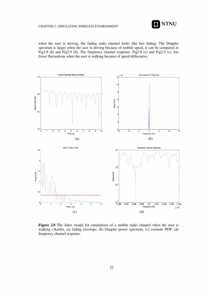
As we could see in section 2.3.2, fading radio channel can be constructed by

summing a set of complex sinusoids. Two different scenarios have been simulated; when the

user is walking (3km/h) and when the user is driving (80km/h), see Fig2.8 (a) and Fig2.9 (a)

respectively. When the user is walking, the fading radio channel is showed as slow fading but


22

NTNU

when the user is driving, the fading radio channel looks like fast fading. The Doppler

spectrum is larger when the user is driving because of mobile speed, it can be compared in

Fig2.8 (b) and Fig2.9 (b). The frequency channel response, Fig2.8 (c) and Fig2.9 (c), has

fewer fluctuations when the user is walking because of speed differences.

0 1 2 3 4 5 6 7 8 9 1010

-2

10-1

100

101

Typical Rayleigh fading envelope

Time (s)

Sig

nal le

vel dB

-15 -10 -5 0 5 10 150

2

4

6

8

10

12

14x 10

5 Tap Frequency Response

Frequency (Hz)

Ma

gn

itu

de

(a) (b)

0 1 2 3 4 5 60

0.5

1

1.5

2

2.5Delay Power Profile

Delay (us)

Ma

gn

itu

de

2.396 2.397 2.398 2.399 2.4 2.401 2.402 2.403 2.404

x 109

10-4

10-3

10-2

10-1


Frequency (Hz)

Magnitude

(c) (d)


walking (3km/h), (a) fading envelope, (b) Doppler power spectrum, (c) estimate PDP, (d)



23

NTNU

0 1 2 3 4 5 6 7 8 9 1010

-2

10-1

100

101

Typical Rayleigh fading envelope

Time (s)

Sig

na

l le

ve

l d

B

-400 -300 -200 -100 0 100 200 300 4000

1

2

3

4

5

6

7x 10

5 Tap Frequency Response

Frequency (Hz)

Ma

gn

itu

de

(a) (b)

0 1 2 3 4 5 60

0.1

0.2

0.3

0.4

0.5

0.6

0.7Delay Power Profile

Delay (us)

Ma

gn

itu

de

2.396 2.397 2.398 2.399 2.4 2.401 2.402 2.403 2.404

x 109

10-2

10-1

100

101


Frequency (Hz)

Ma

gn

itu

de

(d

B)

(c) (d)


driving (80km/h), (a) fading envelope, (b) Doppler power spectrum, (c) estimate PDP, (d)


2.4.3 Different Power Tap Delays

According to different environments exist different PDPs, so different Doppler

spectra have been used for different delays. Urban area, hilly area and flat terrain have been

considered as three sorts of possible environments.


24

NTNU

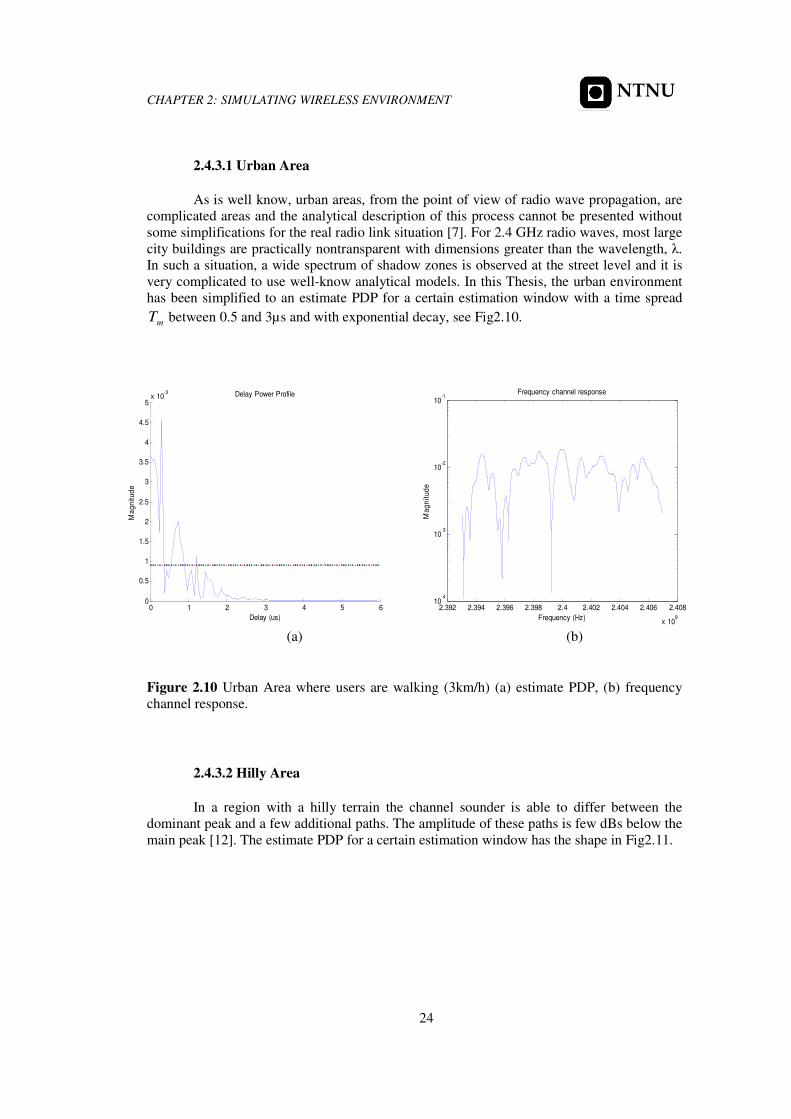
2.4.3.1 Urban Area

As is well know, urban areas, from the point of view of radio wave propagation, are

complicated areas and the analytical description of this process cannot be presented without

some simplifications for the real radio link situation [7]. For 2.4 GHz radio waves, most large

city buildings are practically nontransparent with dimensions greater than the wavelength, λ.

In such a situation, a wide spectrum of shadow zones is observed at the street level and it is

very complicated to use well-know analytical models. In this Thesis, the urban environment

has been simplified to an estimate PDP for a certain estimation window with a time spread

mT between 0.5 and 3µs and with exponential decay, see Fig2.10.

0 1 2 3 4 5 60

0.5

1

1.5

2

2.5

3

3.5

4

4.5

5x 10


Delay (us)

Ma

gn

itu

de

2.392 2.394 2.396 2.398 2.4 2.402 2.404 2.406 2.408

x 109

10-4

10-3

10-2

10-1


Frequency (Hz)

Ma

gn

itu

de

(a) (b)

Figure 2.10 Urban Area where users are walking (3km/h) (a) estimate PDP, (b) frequency

channel response.

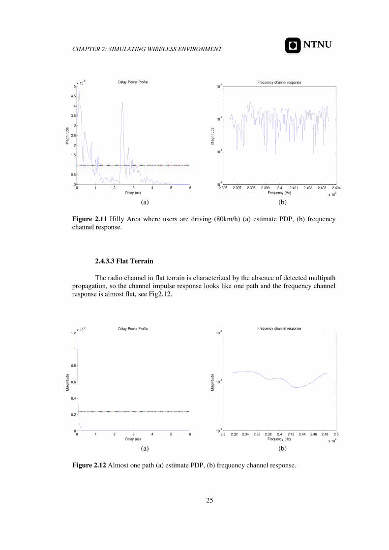
2.4.3.2 Hilly Area

In a region with a hilly terrain the channel sounder is able to differ between the

dominant peak and a few additional paths. The amplitude of these paths is few dBs below the

main peak [12]. The estimate PDP for a certain estimation window has the shape in Fig2.11.


25

NTNU

0 1 2 3 4 5 60

0.5

1

1.5

2

2.5

3

3.5

4

4.5

5x 10


Delay (us)

Ma

gn

itu

de

2.396 2.397 2.398 2.399 2.4 2.401 2.402 2.403 2.404

x 109

10-4

10-3

10-2

10-1


Frequency (Hz)

Ma

gn

itu

de

(a) (b)

Figure 2.11 Hilly Area where users are driving (80km/h) (a) estimate PDP, (b) frequency

channel response.

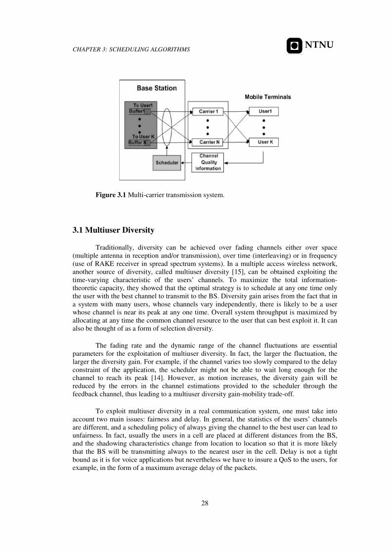
2.4.3.3 Flat Terrain

The radio channel in flat terrain is characterized by the absence of detected multipath

propagation, so the channel impulse response looks like one path and the frequency channel

response is almost flat, see Fig2.12.

0 1 2 3 4 5 60

0.2

0.4

0.6

0.8

1

1.2x 10


Delay (us)

Ma

gn

itu

de

2.3 2.32 2.34 2.36 2.38 2.4 2.42 2.44 2.46 2.48 2.5

x 109

10-4

10-3

10-2


Frequency (Hz)

Ma

gn

itu

de

(a) (b)

Figure 2.12 Almost one path (a) estimate PDP, (b) frequency channel response.


26

NTNU

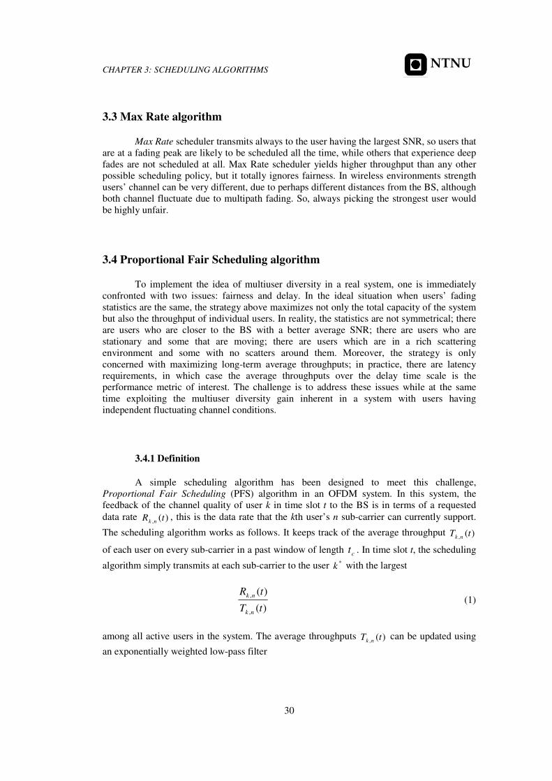
CHAPTER 3: SCHEDULING ALGORITHMS

27

NTNU

Chapter 3

Scheduling Algorithms

In this chapter, different scheduling algorithms have been proposed which are

working in different scenarios. The goal is to improve the throughput of multiple packet-data

users sharing a wireless downlink channel while preserving fairness. RR and Max Rate

algorithms will take into account to improve fairness and throughput respectively and two

proportional fair scheduling algorithms, PFS and RCG which maximize system throughput

maintained fairness. Scheduling algorithms for wireless packet data networks exploit the fact

that the propagation channels between the BS and the MSs it serves fade independently by

scheduling transmission to MSs when their channels are good, giving rise to multiuser

diversity [13].

The system under consideration is an OFDM system with frequency-division

multiple access (FDMA) and time-division multiple access (TDMA). Perfect channel state

information is assumed at both the MS and the BS, i.e. the channel gain on each sub-carrier

due to path loss, shadowing, and multipath fading is assumed to be known.

Each sub-carrier can only be used by one user at any given time. Sub-carrier allocation is

performed at the BS and the users are notified of the sub-carriers chosen for them. Consider a

system with K users, N sub-carriers and the time divided in time slots. At each time slot, each

scheduling user k will transmit on the allocated sub-carrier. Equal power allocation

algorithms are taken in consideration, which simply distributes the transmission power

equally among the sub-carriers. The objective is to find a sub-carrier allocation, which allows

each user to satisfy its rate requirements, maximizing throughput without comprising

fairness. The system is showed in Fig3.1.


28

NTNU

Figure 3.1 Multi-carrier transmission system.

3.1 Multiuser Diversity

Traditionally, diversity can be achieved over fading channels either over space

(multiple antenna in reception and/or transmission), over time (interleaving) or in frequency

(use of RAKE receiver in spread spectrum systems). In a multiple access wireless network,

another source of diversity, called multiuser diversity [15], can be obtained exploiting the

time-varying characteristic of the users’ channels. To maximize the total information-

theoretic capacity, they showed that the optimal strategy is to schedule at any one time only

the user with the best channel to transmit to the BS. Diversity gain arises from the fact that in

a system with many users, whose channels vary independently, there is likely to be a user

whose channel is near its peak at any one time. Overall system throughput is maximized by

allocating at any time the common channel resource to the user that can best exploit it. It can

also be thought of as a form of selection diversity.

The fading rate and the dynamic range of the channel fluctuations are essential

parameters for the exploitation of multiuser diversity. In fact, the larger the fluctuation, the

larger the diversity gain. For example, if the channel varies too slowly compared to the delay

constraint of the application, the scheduler might not be able to wait long enough for the

channel to reach its peak [14]. However, as motion increases, the diversity gain will be

reduced by the errors in the channel estimations provided to the scheduler through the

feedback channel, thus leading to a multiuser diversity gain-mobility trade-off.

To exploit multiuser diversity in a real communication system, one must take into

account two main issues: fairness and delay. In general, the statistics of the users’ channels

are different, and a scheduling policy of always giving the channel to the best user can lead to

unfairness. In fact, usually the users in a cell are placed at different distances from the BS,

and the shadowing characteristics change from location to location so that it is more likely

that the BS will be transmitting always to the nearest user in the cell. Delay is not a tight

bound as it is for voice applications but nevertheless we have to insure a QoS to the users, for

example, in the form of a maximum average delay of the packets.


29

NTNU

3.1.1 Multiuser Diversity and Mobility

It is clear that for pedestrian speeds diversity gain is the main phenomenon involved.

However, as velocity of the users increases, the loss in performance is dramatic. As the

Doppler spread, λ/vf d = increases, the coherence time of the channel becomes shorter,

and the rate request is less reliable. Fast fading may affect not only multiple-slot packets, but

also single-slot ones. In fact, it can happen that the rate requested based on the pilot channel

measurement made in the previous slot is not supported by the channel in the actual slot, and

thus the packet can be lost.

As the speed of the users increases, this measured SNR is a less reliable prediction of

the current state of the channel. Suppose we split the slot into two semi-slots, each with a

pilot channel (of half length). This would double the feedback channel rate, but not result in a

dramatic increase in the amount of data (with 4 bits we can address the 11 rates that the

mobiles can request on the feedback channel). Naturally, the number of slots per packet is

doubled, but the packets have the same duration in time. Hence we can now better exploit the

multiuser diversity effect and, at the same time, reduce the impact of the coherency of the

channel for high speeds. In fact, the pilot measurement is a more accurate prediction of the

channel state because it is carried out twice as often. Also, if the packet duration is more than

one slot, one can better adapt the transmission to the fading characteristics of the channel.

Suppose we are transmitting the ith slot of an n-slots packet at a rate kR , and that for the

current slot the rate request of the user is iR <

kR . One can avoid transmitting the n-i slots

remaining, because they would probably be lost. Instead, we stop the transmission to the user

(completing only the current slot), and restart the proportional fair algorithm for the

assignment of the downlink. To ensure fairness, the fairness index is not computed on the

whole packet, but only on the basis of the actual data transmitted to the MS (i slots in this

case). The improvement is large, and the cost is only a small amount of additional

information to feedback to the BS.

3.2 Round Robin algorithm

Round Robin (RR) is one of the simplest scheduling algorithms, which assigns time

slices to each MS in equal portions and in order, handling all MSs as having the same

priority. RR scheduling is both simple and easy to implement, and starvation-free.

In wireless networks, where many stations share one channel, this algorithm provides

every MS to transmit or receive on the shared channel at a regular interval. This may make

RR to appear a fair algorithm. However, because it is much less efficient than other

algorithms such as PFS or RCG (as we will see in sections 3.4 and 3.4 respectively), hardly

will provide very good service to the MS. The BS will also suffer reduced capacity of the

network. The main reason for this is that this algorithm does not take into account the

changing reception conditions at the different receivers or as we said before, RR algorithm

does not take into account multiuser diversity and thus it will schedule transmissions to/from

subscribers half of the time when their reception conditions are worse than average [17].


30

NTNU

3.3 Max Rate algorithm

Max Rate scheduler transmits always to the user having the largest SNR, so users that

are at a fading peak are likely to be scheduled all the time, while others that experience deep

fades are not scheduled at all. Max Rate scheduler yields higher throughput than any other

possible scheduling policy, but it totally ignores fairness. In wireless environments strength

users’ channel can be very different, due to perhaps different distances from the BS, although

both channel fluctuate due to multipath fading. So, always picking the strongest user would

be highly unfair.

3.4 Proportional Fair Scheduling algorithm

To implement the idea of multiuser diversity in a real system, one is immediately

confronted with two issues: fairness and delay. In the ideal situation when users’ fading

statistics are the same, the strategy above maximizes not only the total capacity of the system

but also the throughput of individual users. In reality, the statistics are not symmetrical; there

are users who are closer to the BS with a better average SNR; there are users who are

stationary and some that are moving; there are users which are in a rich scattering

environment and some with no scatters around them. Moreover, the strategy is only

concerned with maximizing long-term average throughputs; in practice, there are latency

requirements, in which case the average throughputs over the delay time scale is the

performance metric of interest. The challenge is to address these issues while at the same

time exploiting the multiuser diversity gain inherent in a system with users having

independent fluctuating channel conditions.

3.4.1 Definition

A simple scheduling algorithm has been designed to meet this challenge,

Proportional Fair Scheduling (PFS) algorithm in an OFDM system. In this system, the

feedback of the channel quality of user k in time slot t to the BS is in terms of a requested

data rate )(, tR nk, this is the data rate that the kth user’s n sub-carrier can currently support.

The scheduling algorithm works as follows. It keeps track of the average throughput )(, tT nk

of each user on every sub-carrier in a past window of length ct . In time slot t, the scheduling

algorithm simply transmits at each sub-carrier to the user *k with the largest

)(

)(

,

,

tT

tR

nk

nk (1)

among all active users in the system. The average throughputs )(, tT nk can be updated using

an exponentially weighted low-pass filter


31

NTNU

≠

−

=+

−

=+

)()(1

1

)()(1

)(1

1

)1(

*

,

*

,,

,

tkktTt

tkktRt

tTt

tT

nk

c

nk

c

nk

c

nk (2)

In this report, the PFS algorithm in an OFDM system is used taken sub-carriers

independently each other. So, we have to compute what user has the largest value given by

equation (1) at each sub-carrier and time slot in order to allocate this sub-carrier to that user.

Also, we have to update the users’ average throughput by equation (2) at each sub-carrier and

time slot. So, the PFS algorithm treats sub-carriers independently each other and we have to

update the system every time slot. This algorithm does not take into account users’ rate

requirements and conventional power allocation is not considered because it has some weak

points that degrade the system performance when employed in heterogeneous user channel

environment [31]. Equal power allocation algorithm is taken in consideration, which simply

distributes the transmission power equally among the sub-carriers. To exploit the flexibility

of transmission power allocation which is inherent in multiuser OFDM systems we

encourage reader to see [31].

One can get an intuitive feel of how this algorithm works by inspecting Fig3.2. We

plot the frequency channel response of two users as a function in two different scenarios,

equal and unequal fading statistics. In Fig3.2 (a), the two users have identical fading

statistics. If the scheduling time scale ct is much larger than the correlation time scale of the

fading dynamics, then by symmetry the throughput of each user converges to the same

quantity. The scheduling algorithm reduces to always picking the user with the highest

requested rate. Thus, each user is scheduled when its channel is good and at the same time the

scheduling algorithm is perfectly fair on the long term. In Fig3.2 (b), due to perhaps different

distances from the BS, one user’s channel is much stronger than the other user’s on the

average, although both channels fluctuate due to multipath fading. Always picking the user

with the highest requested rate means giving all the system resources to the statistically

stronger user and would be highly unfair. In contrast, under the proposed scheduling

algorithm, users compete for resources not directly based on their requested rates but only

after normalization by their respective average throughputs. The user with the statistically

stronger channel will have a higher average throughput. Thus, the algorithm schedules a user

when its instantaneous channel quality is high relative to its own average channel condition

over the time scale ct . In short, data is transmitted to a user when its channel is near its own

peaks. Multiuser diversity benefit can still be extracted because channels of different users

fluctuate independently so that if there is a sufficient number of users in the system, there will

likely be a user near its peak at any one time.


32

NTNU

2.394 2.396 2.398 2.4 2.402 2.404 2.406

x 109

0

0.01

0.02

0.03

0.04

0.05

0.06

0.07

0.08Frequency channel response

Frequency (Hz)

Magnitude

user A

user B

2.394 2.396 2.398 2.4 2.402 2.404 2.406

x 109

0

0.02

0.04

0.06

0.08

0.1

0.12

0.14

0.16


Frequency (Hz)

Magnitude

user A

user B

(a) (b)

Figure 3.2 Frequency channel response (a) equal users, (b) unequal users.

3.4.2 The Parameter ct

The parameter ct is tied to the latency time scale of the application. Peaks are defined

with respect to this time scale. If the latency time scale is large, then the throughput is

averaged over a longer time scale and the scheduler can afford to wait longer before

scheduling a user when its channel hits a really high peak [18].

The larger value of ct parameter is ct =∞, in this situation the allocation resources

according to PFS algorithm is decided solely by instantaneous SNR, leading to maximum

system throughput and poor fairness characteristics. On the other hand, the lower value of ct

parameter is ct =1 in this situation scheduling becomes fair. Therefore,

ct means the trade-

off between fairness and throughput. Table 3.I shows simulation parameters. The

performance of this algorithm is analyzed and compared through MATLAB computer

simulations with throughput_fairness_Vs_PFS.m file, see Appendix C.3.

Time slots 100

Sub-carriers 16

ct From 1 to 1000

Users 4

Mobile Speed (km/h) 3

Table 3.I Simulation parameters


33

NTNU

In Fig3.3 (a), the system fairness is showed, F, versus ct parameter according to

three different algorithms, PFS, RR and Max Rate. As we will see in chapter 4, if F=1 all

users share exactly the same amount of resources, and F=0 occurs when only one user

consumes all amount of resources. Max Rate and RR algorithms are independently of

ct parameter, so fairness according to these algorithms remains constant and represents

fairness’ boundaries. Max Rate algorithm represents the smallest fairness and RR algorithm

represents the largest fairness. As we can see in Fig3.3 (a) if ct tends to 1, there is an

increase in fairness and PFS behaviour tends to RR behavior, but if ct tends to infinity, there

is a reduction in fairness and PFS behavior tends to Max Rate behaviour.

On the other hand, in Fig3.3 (b) throughput versus ct parameter is showed. As we

have said before, Max Rate and RR algorithms are independently of ct parameter and

represent behaviour’s boundaries. Max Rate algorithm represents the largest throughput and

RR algorithm represents the smallest throughput. As we can see in Fig3.3 (b) if ct tends to

infinity, there is an increase in throughput and PFS behaviour tends to Max Rate behavior,

but if ct tends to 1, there is a reduction in throughput and PFS behavior tends to RR

behaviour.

0 100 200 300 400 500 600 700 800 900 10000

0.2

0.4

0.6

0.8

1

System Fairness: PFS Vs Max SNR

tc

Fa

irn

es

s

0 100 200 300 400 500 600 700 800 900 10002

4

6

8

10

12

14

16x 10

5 System Capacity

tc

Th

rou

gh

pu

t (b

ps

)

(a) (b)

Figure 3.3 PFS (dotted line), RR (dotted continuous line) and Max Rate (continuous line)

behaviour versus ct parameter (a) fairness, (b) throughput.


34

NTNU

3.5 Rate-Craving Greedy algorithm

This algorithm divides the problem of joint allocation into two steps. In the first step,

the number of sub-carriers that each user will get is determined based on the users’ rate

requirements and average SNR. The algorithm is shown to find the distribution of sub-

carriers that minimizes the total power required when every user experiences a flat-fading

channel. In the second stage of the algorithm, it finds the best assignment of sub-carriers to

users based on the estimated rate of transmission.

Consider a system with K users and N sub-carriers. Each user k must transmit at least k

Rmin bits per unit time to satisfy rate requirements. A user can transmit at most

maxR bits per

unit time and sub-carrier, so maxR is the maximum value that the user’s subchannel response

reaches. Let )(, tH nk be the channel gain and )(, tr nk

the transmission rate for user k on sub-

carrier n at t time slot.

The objective is to find a sub-carrier allocation, which allows each user to satisfy its

rate requirements.

As we said before, the problem is solved by two algorithms, which use information

about users’ channel and rate requirements to find a close approximation to the solution.

1. Resource Allocation: Decide the number of sub-carriers each user gets - its

bandwidth - based on rate requirements and the users’ average channel gain, Band

Assignment Based on SNR (BABS) algorithm.

2. Sub-carrier Allocation: Use the result of the resource allocation stage and channel

information to allocate the sub-carriers to the users, Rate Craving Greedy (RCG)

algorithm.

By solving these sub-problems separately, a good, but not necessarily optimal,

solution is found which guarantees a certain level of service for each user.

3.5.1 BABS

This section describes the bandwidth assignment based on SNR, BABS algorithm

which uses the rate requirements and the average SNR for each user to decide the number of

sub-carriers that user will be assigned.

Assume that each user k experiences a channel gain of ( )∑−

==

1

0

2

,, /)()(N

n nknk NtHtH

on every sub-carrier. Let user k be allocated km sub-carriers. When the gain on every sub-

carrier is the same, the optimal rate-power allocation is to transmit k

kmR /min

bits on each sub-

carrier.


35

NTNU

To find the optimal distribution of sub-carriers among users given the flat channel

assumption, a greedy descent algorithm is proposed.

3.5.1.1 BABS ALGORITHM

The implemented BABS algorithm works as follow: At first each user gets km sub-

carriers according to their rate requirements, if the sum of the whole sub-carriers allocated

does not fit with the available bandwidth, we have to

1. remove sub-carriers from users who are demanding less sub-carriers.

2. add sub-carriers to users according to the SNR.

In [16], this algorithm is shown to converge to the distribution of sub-carriers

among users and the function f(r) is explained more accurately. In order to make

relevant comparisons with the other algorithms, fix power at the BS is used. So, the

BS simply distributes the transmission power equally among the sub-carriers without

taking advantage on power control.

whileend

mm

Gl

Kkm

Rf

H

m

m

Rf

H

mG

doNmwhile

whileend

m

mk

doNmwhile

KkR

Rm

ll

kKk

k

k

k

k

k

k

k

k

k

K

k k

k

kKk

K

k k

k

k

1

minarg

1,...,0,1

1

,

0

minarg

1,...,0,

10

minmin

1

0

10

*

1

0

max

min

*

+←

←

−=

−

+

+←

<

←

←

>

−=

←

−≤≤

−

=

−≤≤

−

=

∑

∑


36

NTNU

3.5.2 RCG

Once the number of sub-carriers is determined, the next step is to assign specific sub-

carriers to users. The problem is still difficult to solve since different users see different

channels. The RCG algorithm begins with an estimate of the users’ transmission rate on each

sub-carrier and aims to maximize the total transmission rate. For the model used in

simulations )1(log/)( 2, SNRNBtr nk += is used, according to Shannon capacity theorem.

3.5.2.1 RCG ALGORITHM

The algorithm works as follow:

1. Allocate each sub-carrier n at each time slot to the user with maximum transmission

rate )(, tr nk.

2. While there exists some user k such that the number of sub-carriers allocated

according to maximum transmission rate are more than km , the sub-carriers

allocated according to BABS algorithm, remove a sub-carrier from user k and

add a sub-carrier to user l such that the number of sub-carriers allocated

according to maximum transmission rate are less than km , using a sequence

of reallocations.

{ }

{ }

{ } { }

forend

whileend

nCCnCC

nrnrn

nrnrl

domnumCwhile

domnumCthatsuchkusersallfor

forend

nCC

nrk

doNnsubcarriereachfor

llkk

lkNn

lkNnmnumCl

kk

kk

kk

kKk

kk

**

10

*

10:

*

10

*

**

*

**

,/

)()(minarg

)()(minminarg

,

,

)(maxarg

,1:0

∪←←

+−←

+−←

>

>

∪←

←

−=

−≤≤

−≤≤<

−≤≤


37

NTNU

3.5.3 Example Run of the Algorithm

In this section an example run of the algorithm is demonstrated for N=8 sub-carriers

and K=4 users which require 64, 45, 35 and 16 Kb per time slot, see Table 3.II (a).

At first the algorithm decides the number of sub-carriers each user gets base on rate

requirements and the users’ average channel gain. As we can see in Table 3.II (b), the number

of sub-carriers demanded does not fit with the available bandwidth, so the sub-carriers are

removed from the users who are demanded less transmission rate until the number of sub-

carriers allocated to users would be 8, Table 3.II (c).

Demanded

transmission rate

Demanded sub-

carriers

Allocated sub-

carriers

#1 64 3 3

#2 45 3 2

#3 16 2 1

#4 35 3 2

(a) (b) (c)

Table 3.II (a) Transmission rate demanded by users, (b) sub-carriers demanded by users, (c)

sub-carriers allocated by the algorithm.

Once the number of sub-carriers is determined, this information and channel state are

used to allocate the sub-carriers to the users.

#1 #2 #3 #4

#1 4 1 2 3

#2 7 6 3 5

#3 6 2 4 1

#4 5 8 1 8

#5 3 4 6 2

#6 8 7 8 6

#7 2 3 5 4

#8 1 5 7 7

(a) (b)

Table 3.III Sub-carrier allocation by RCG algorithm at the end of stage 1 (a) and (b) the

algorithm. The number in column k row n is the estimated rate of transmission of user k on

sub-carrier n, if it is allocated that sub-carrier. The blond rate has been chosen.

#1 #2 #3 #4

#1 4 1 2 3

#2 7 6 3 5

#3 6 2 4 1

#4 5 8 1 8

#5 3 4 6 2

#6 8 7 8 6

#7 2 3 5 4

#8 1 5 7 7


38

NTNU

In Table 3.III, columns represent different users, rows are different sub-carriers. The

number in row n column k represents an estimate of the rate at which user k would transmit

on n if it were allocated that sub-carrier. The blond numbers show to whom each sub-carrier

is allocated.

1. Allocate each sub-carrier n to the user with the maximum transmission rate.

User #1 → 4 sub-carriers




2. Because of there exits some users such that the number of sub-carriers

allocated according to Max Rate is more than the number of sub-carriers

allocated according to BABS algorithm, sub-carriers are removed from these

users and add to others according to Table 3.II (c).

Remove one sub-carrier from user #1 to user #4

Remove two sub-carriers from user #3, one to user #2 and one to user #4

In Appendix G, we can see an example run of this algorithm in 10 different time slots

with equal and unequal users.


In this section two different scheduling policies have been compared for system

resources allocating, PFS and RCG. Also, RR and Max Rate algorithms have been used for

reinforcing the conclusions about system fairness and throughput.

The algorithms will be compared based on three criteria, fairness, throughput and

delay but these results will be show in chapters 4, 5 and 6 respectively. In this chapter the

policies used for allocating resources will be showed. The performance of these algorithms is

analyzed and compared through MATLAB computer simulations with scheduler.m and

statistic.m files, see Appendix C.1 and C.2 respectively.

3.6.1 Model Description

In this report, the downlink transmission of a multiuser OFDM system is considered.

We assume that the overall bandwidth B is divided into N orthogonal narrow-band sub-

carriers. Each MS measures the channel gain of each sub-carrier and feeds back the channel

state information to the BS via a separate feedback channel. We assume that channel

estimation can be done perfectly and feedback channel is errorless. The data stream of each


39

NTNU

selected user is then modulated by a proper modulation scheme that is supportable in the

given channel state and the allocated transmission power of the sub-carrier.

In the frequency selective fading channel, in general, different sub-carriers

experience different channel gains even for the same user. We assume that each sub-carrier is

narrow enough to undergo flat fading. We also assume that the channel gain is constant in

each time slot but varies from slot to slot. Under the assumptions above, the received SNR of

the nth sub-carrier signal of the kth user at the tth slot can be expressed by

NBN

tHtStSNR

nknk

nk/

)()()(

0

,,

, = (3)

where )(),( ,, tHtS nknk are the allocated transmission power and channel gain on nht sub-

carrier at tth time slot respectively, 0N is the power spectral density of AWGN, B is the

bandwidth and N is the number of sub-carriers.

In multiuser OFDM systems, a resource allocation algorithm decides which user to

serve with what power for each sub-carrier. Here, is assumed that the total transmission

power is constrained to S . Once the resources are allocated to users, the instant data rate of

each user is determined and the BS serves each user at this rate. According to information

theory and as we can see in Chapter 5, the instant service rate on the nth sub-carrier at tth

time slot is got by

)1(log/)( 2, SNRNBtR nk += (4)

where )(, tR nk is the kth user transmission rate at tth time slot, B is the total bandwidth and N

is the number of sub-carriers.

Three classes of services are considered: data, voice, and video. It is assumed that

10% of the users will be transmitting video, 40% will be transmitting voice, and the

remaining 50% of the users will be transmitting data. Video and voice traffic are given a

constant transmission rate of 64 and 16 Kb per time slot, respectively, whereas data traffic is

assumed to be exponentially distributed, with a mean of 30 Kb per time slot.

3.6.2 Simulation Results

In simulations there are 16 sub-carriers for the OFDM system and the carrier

frequency is 2.4 GHz. In order to show how work the different scheduling algorithms we

only simulate four different users, A (red), B (blue), C (green) and D (yellow), with their

different channel responses. We assume that user A is transmitting video (64 Kb per time

slot), user B is transmitting voice (16 Kb per time slot), users C and D are transmitting data,

30 and 40 Kb per time slot respectively. Each sub-carrier is allocated to each user in two


40

NTNU

different scenarios according to four different algorithms, RR, Max Rate, PFS and RCG.

Table 3.IV shows simulation parameters.

Time slots 16

Sub-carriers 16

fc (GHz) 2.4

ct 20 and 100’000

Users 4

Rates (Kb per time slot) 16, 30, 40 and 64


Table 3.IV Simulation parameters.

2.395 2.396 2.397 2.398 2.399 2.4 2.401 2.402 2.403 2.404 2.405

x 109

0

0.005

0.01

0.015

0.02

0.025

0.03

0.035

0.04

0.045


Frequency (Hz)

Magnitude

2.395 2.396 2.397 2.398 2.399 2.4 2.401 2.402 2.403 2.404 2.405

x 109

0

0.02

0.04

0.06

0.08

0.1

0.12


Frequency (Hz)

Magnitude

(a) (b)

Figure 3.4 Frequency channel response at any instant time it , (a) equal users, (b) unequal users.

3.6.2.1 Scenario A: Equal Users

As we can see in Fig3.4 (a), all the users simulated have the same channel response

average. In Fig3.5, the scheduler scheme is showed according to four different scheduling

policies.

As we can see in Fig3.5 (a), RR algorithm allocates all sub-carriers to one user at

each time slot, so this policy is totally fair. In this scenario we cannot notice the differences

between Max Rate (see Fig3.5 (b)) and PFS (see Fig3.5 (c)) policies on allocating resources


41

NTNU

because all users have the same channel response average. But we can notice that RCG

allocates more sub-carriers to user A than other scheduling algorithms, the reason is because

only this algorithm takes into account rate requirements by users and user A is transmitting

video and this services needs more amount of data than other services, so user A needs more

sub-carriers than other users.

0 2 4 6 8 10 12 14 16 18

0

2

4

6

8

10

12

14

16

18

Subchannel allocation according to Round Robin

Time slots

Sub-c

arr

iers

0 2 4 6 8 10 12 14 16 18

0

2

4

6

8

10

12

14

16

18

Subchannel allocation according to Max Rate

Time slots

Sub-c

arr

iers

(a) (b)

0 2 4 6 8 10 12 14 16 18

0

2

4

6

8

10

12

14

16

18

Subchannel allocation according to PFS

Time slots

Sub-c

arr

iers

0 2 4 6 8 10 12 14 16 18

0

2

4

6

8

10

12

14

16

18

Subchannel allocation according to RCG

Time slots

Sub-c

arr

iers

(c) (d)

Figure 3.5 Scheme where users have equal channel responses average and have been

simulated according to filtered Gaussian noise method, (a) RR algorithm, (b) Max Rate

algorithm, (c) PFS algorithm, with ct =20, (d) RCG algorithm.


42

NTNU

3.6.2.2 Scenario B: Unequal Users

As we can see in Fig3.4 (b), the user A (red) is nearer to the BS than the other users

because the channel A is stronger than others. In this scenario RR algorithm (see Fig3.6 (a))

takes the same scheduler scheme that the previous scenario, it allocates system resources to

one user at each time slot.

When users have not the same channel response average, we can notice the

differences between Max Rate and PFS on scheduling resources and the different PFS

scheduler scheme when ct parameter changes. As we can see in Fig3.6 (b), almost all sub-

carrier are allocated to user A because of channel strength and the same results are achieved

with PFS policy when ct parameter is high (see Fig3.6 (c)) but, as we saw in section 3.4.2 the

results change when we take a low ct parameter (see Fig3.6 (d)). The larger ct parameter, the

unfairer PFS is.

RCG policy maintenances the index fairness because RCG allocates sub-carriers

based on rate requirements and the users’ average SNR.

0 2 4 6 8 10 12 14 16 18

0

2

4

6

8

10

12

14

16

18

Subchannel allocation according to Round Robin

Time slots

Sub-c

arr

iers

0 2 4 6 8 10 12 14 16 18

0

2

4

6

8

10

12

14

16

18

Subchannel allocation according to Max Rate

Time slots

Sub-c

arrie

rs

(a) (b)


43

NTNU

0 2 4 6 8 10 12 14 16 18

0

2

4

6

8

10

12

14

16

18


Time slots

Sub-c

arrie

rs

0 2 4 6 8 10 12 14 16 18

0

2

4

6

8

10

12

14

16

18


Time slots

Sub-c

arrie

rs

(c) (d)

0 2 4 6 8 10 12 14 16 18

0

2

4

6

8

10

12

14

16

18

Subchannel allocation according to RCG

Time slots

Sub-c

arrie

rs

(e)

Figure 3.6 Scheme scheduled where users have unequal channel responses average and have


algorithm, (c) PFS algorithm, with ct =20, (d) PFS algorithm, with ct =100’000, (e) RCG

algorithm


44

NTNU

CHAPTER 4: FAIRNESS

45

NTNU

Chapter 4

Fairness

In this chapter, one of the most important properties in a wireless environment where

system resources are being shared by users is discussed. In order to evaluate and find the

scheduling disciplines with the best performance, appropriate performance measures are

required. For best effort users the major concern for the scheduling discipline should be to

maximize the total throughput for all users at the same time as each user is served a fair

amount of throughput.

4.1 Definition

Fairness is a desirable property of the wireless network as it offers protection

between users. This means than the traffic flow of an ill-behaving user cannot affect the

traffic flow of another user.

The fairness of a system, the users in a system, or of a scheduling algorithm is not

usually expressed in terms of a quantitative value. Rather, fairness is usually expressed in

broader terms. Generally, a system is deemed to be fair or unfair based on whether or not the

system meets certain criteria. Such criteria are usually in terms of throughput or delay. For

example, a scheduling algorithm may be deemed to be unfair if any user receives a

throughput of less than X bits/sec. Another example might be that a system is deemed fair if

the probability of any user experiencing a delay greater than τ is less than p; if the probability

is greater than p the system is unfair. The rationale behind the proposed definitions is to see if

a value for the “fairness” of a system or scheduling algorithm can be defined in a similar

manner to how Shannon defined a value for the “information” of a source. The fairness value

should also make sense from both a mathematical and a semantic sense. Shannon’s definition

was based on probabilities of events. In comparison, the proposed fairness measures are

based on proportions of allocated resources [20]. In order to evaluate fairness, we propose

two set of users, equal and unequal weighted users.

CHAPTER 4: FAIRNESS

46

NTNU

4.2 Equal weighted users

The “resources” in question depend on the circumstances under which the definition

is applied. Possible examples include the number of bits or packets sent to users, or the

amount of bandwidth, time, or slots each user is allocated. The proportion for each user

would then be the number or amount of packets, bandwidth, slots, etc. allocated to that user,

relative to the total allocated to all the users in the system.

For a random variable or process X, the self-information of the event X= ix is:

)(log)(

1log)( i

i

i xPxP

xI −== (1)

where P( ix ) is the probability of the event X= ix .

A measure for fairness can be defined in a similar manner, but using proportions

instead of probabilities. In the case when all N users of a system are considered equal, the

definition for the “self-fairness” of a given user is:

N

p

N

pF ii

ilog

log

)/1log(

log−=

−

−= (2)

where ip , is the proportion of resources allocated to user i, and the logN term is a

normalization factor. The “self-unfireness” of a user can also be defined simply as the

reciprocal of the self-fairness:

ii

ip

N

FU

log

log1 −== (3)

4.2.1 Average fairness and average unfariness

Given the self-information of the N possible events of the process X as given by, the

average self-information in the process X can be found by:

∑ ∑= =

−==N

k

N

k

kk

k

k xPxPxI

xPXH

1 1

)(log)()(

)()( (4)

Similarly, the proposed definition for the “average fairness” of a system of N users

is:

CHAPTER 4: FAIRNESS

47

NTNU

∑ ∑= =

−==N

k

N

k

k

kkkN

ppFpF

1 1 log

log (5)

And the “average unfairness” is given by:

∑ ∑= =

−==N

k

N

k k

kkkp

NpUpU

1 1 log

log (6)

4.2.2 Remarks

The above definitions yield some interesting properties:

1. When a user consumes exactly its fair share of resources (i.e. a proportion of 1/N),

the value of self-fairness and self-unfairness for that user will be unity.

2. As the amount of resources a user consumes increases, it takes an increasing amount

away from the other users in the system. Thus, that user becomes less fair (or more

unfair), and consequently, the values of self-fairness and self-unfairness for that user

decrease and increase respectively.

3. Conversely, as a user consumes fewer resources, it is giving up resources in favor of

the other users in the system. Hence, that user becomes much fair (or less unfair), and

correspondingly, the values of self-fairness and self-unfairness for that user increase

and decrease respectively.

4. In the limit as one user consumes all the available resources, all the other users in the

system will be the greedy user to be less fair (or more unfair). Thus, logically, the

value for the self-unfairness for that user should be the highest possible value,

infinity, which indeed proves to be the case in the proposed definition. The self-

fairness for the user in question becomes zero, the lowest value the self-fairness can

become.

5. Similarly, in the limit when a user consumes no resources, that user gives up all its

deserved resources in favor of other users. Thus, there is no possible way for that

user to be much fair (or less unfair). This is reflected in the resulting values of

infinity and zero for the self-fairness and self-unfairness, respectively.

6. The value for the average fairness of the system of N users ranges from 0 to 1

inclusive. Furthermore, the maximum value of unity is only achieved when all users

in the system consume exactly their fair share of the resources

(i.e. Nppp N /1...21 ==== ). The minimum of zero occurs in the limit when one

user consumes all the allocated resources while the other N-1 users are starved.

CHAPTER 4: FAIRNESS

48

NTNU

7. Similarly, the average unfairness ranges between 1 and infinity, with the lower and

upper extreme values occurring under the same conditions as the maximum and

minimum values respectively for the average fairness. That is, a value of unity will

result only if all users consume their fair share of resources, and infinity will result if

a single user consumes all the allocated resources.

4.3 Unequal weighted users

The above definitions are now extended to the more general case when individual

users can have different weightings (for example, to achieve different levels of QoS). In [21],

the authors state that for a system of N users with a set of backlogged flows B(t) during the

time interval [21 , tt ] a queuing system is fair if:

0),(),(

),,(,2121

21 =−∈∀j

j

i

i

r

ttW

r

ttWttBji (7)

where Wj, is the capacity granted to flow j (i.e. the resources allocated to flow j), and jr is the

weighting of user j. From this, it can be shown that the proportion of the resources allocated

to user j that is deemed to be fair (in other words, the proportion of the resources that user j

should receive in order for the system to be fair) is given by:

T

j

jfairr

rP =, (8)

where Tr is the weighting sum of all users. From the above proportion, it can be deduced that

the formula for the weighted self-fairness of a user should become:

Tj

j

jrr

pF

/log

log= (9)

The weighted self-unfairness of a user is the reciprocal of the above equation:

j

Tj

jp

rrU

log

/log= (10)

CHAPTER 4: FAIRNESS

49

NTNU

4.3.1 Weighted Average fairness and unfariness

It would be desirable to define the weighted average fairness as∑ =

N

k kk Fp1

, as in the

case of equal weighted users. However, it is impossible to make this definition and still

maintain the properties discussed before. Instead, the weighted average fairness of a system

can be defined as:

∑

∑

=

==N

k

kk

N

k

kkkT

rC

FpCr

F

1

1 (11)

the values kC are normalization constants.

)/ln(

11

)/ln(

11

1

Tk

T

k

rr

rrC

+

+

= (12)

Their purpose is to ensure that the maximum value of the weighted average fairness is unity

(as in the case of equally weighted users), and that the maximum occurs when user consume

exactly its fair share of the resources (for more details see [20]).

4.3.2 Remarks

The above definitions yield some interesting properties:

1. The weighted definitions share all the same properties as the equal weighted

definitions. The only difference is that the value of 1 occurs for weighted self-

fairness, self-unfairness, average fairness, and average unfairness whenTkk rrp /= ,

k=1,2, ...,N, instead of Npk /1= as before.

2. Note that there is an implicit time scale in the proportions. That is, the proportions of

resource allocation would be measured over a certain period of time. Since the period

used can be arbitrary, the proposed measures can be used to examine both the short-

term fairness and the long-term fairness of systems [19].

CHAPTER 4: FAIRNESS

50

NTNU


In this section the algorithms will be compared based on fairness criteria. We use RR

algorithm as reference because this policy achieves the best results on index fairness.

The performance of these algorithms is analyzed and compared through MATLAB

computer simulations with fairness.m and throughput_fairness_Vs_users.m files, see

Appendix D.1 and Appendix E.1 respectively.


The same system model described in chapter 3 is used. For evaluating the index

fairness, users with different channel response averages in three different scenarios are

considered:

A. All users are transmitting voice, constant rate, 16 Kb per time slot.

B. All users are transmitting video, constant rate, 64 Kb per time slot.

C. Mix scenario where 10% of users are transmitting video, constant rate, 64

Kb per time slot, 40% of users are transmitting voice, constant rate, 16 Kb

per time slot and 50% of users are transmitting data, exponentially

distributed rate, with a mean of 30 Kb per time slot.

Table 4.I shows simulation parameters.

Time slots 100

Sub-carriers 16

ct 20

Users From 5 to 25

Rates (Kb per time slot) 16, 64 and exprnd(30)




MATLAB appears to be a simple and straightforward tool to demonstrate the concept

of fairness. The simulations results are showed in Fig4.1. As we said in section 4.3.2 the

period of time over we can measure the index fairness can be arbitrary, but as the simulation

CHAPTER 4: FAIRNESS

51

NTNU

is so short, the whole set of 100 time slots are used to evaluate the index fairness. So, in this

case the proposed measures are used to examine the short-term fairness which can be

interested for applications with strength delay restrictions.

5 10 15 20 25

0

0.1

0.2

0.3

0.4

0.5

0.6

0.7

0.8

0.9

1

Users

Fairness

System Fairness

RCG

Max Rate

PFS

RR

5 10 15 20 25

0

0.1

0.2

0.3

0.4

0.5

0.6

0.7

0.8

0.9

1

Users

Fairness

System Fairness

RCG

Max Rate

PFS

RR

(a) (b)

5 10 15 20 25

0

0.1

0.2

0.3

0.4

0.5

0.6

0.7

0.8

0.9

1

Users

Fairness

System Fairness

RCG

Max Rate

PFS

RR

(c)

Figure 4.1 System fairness versus users with different channel response average in three

different scenarios, (a) scenario A, (b) scenario B, (c) scenario C.

CHAPTER 4: FAIRNESS

52

NTNU

Max Rate policy is the unfairnest algorithm because it allocates the system resource

to users who have the strongest channel, so the results achieved by this algorithm are

independent from the scenario simulated. As we can see in Fig4.1, the larger the users who

are demanding service in the system, the lower the index fairness, because Max Rate

scheduler always serves to the same stronger users.

As Max Rate scheduler, PFS scheduler is independent from rate requirements, so the

results achieved in these three different scenarios are more or less the same. As we can see in

Fig4.1, PFS algorithm has a good behaviour because as we saw in chapter 3, with a low ct

parameter this algorithm maintenance index fairness without involving system throughput.

As we said in chapter 3, RCG algorithm allocates sub-carriers to users according to

users’ channel response and rate requirements. In Fig4.1, we can see that the larger the users

in the system, the lower the index fairness, but there are differences among them. In the

scenario A, Fig4.1 (a), RCG maintenances total fairness until the number of users in the

system is more than 10 so long as in B scenario, Fig4.1 (b), RCG maintenances total fairness

until 5 users. The reason of this behaviour is because when there are sub-carriers enough to

satisfy rate requirements RCG allocates the share amount of resources among users, but when

there are not sub-carriers enough, RCG algorithm allocates sub-carriers to stronger users until

satisfying their rate requirements, after that RCG allocates the sub-carriers remained. Users

who are demanding video service need more sub-carrier than users who are demanding voice

service, so when there are not sub-carriers enough, users who are transmitting voice have to

wait. In the scenario C, Fig4.1 (c), an intermediate situation in a mix scenario is plotted.

CHAPTER 5: THROUGHPUT

53

NTNU

Chapter 5

Throughput

There is a considerable interest within the industry in specifying the performance of

wireless data. In this chapter, we will discuss about one of the most important properties of

information system, throughput. The throughput is commonly considered within a framework

that optimizes the system performance [22] and is a measure of how much information can be

transmitted and received per unit time with a negligible probability of error. We will evaluate

and find the scheduling disciplines with the best performance.

5.1 Motivation

To design and deploy a WLAN, an accurate deployment procedure is required to

ensure sufficient coverage and network functionality (capacity, interference, etc.). While

wireless networking gear is often classified according to its standards-based signaling rate,

the actual data throughput, or data being transmitted, is often just a fraction of the signaling

rate’s theoretical maximum. Research conducted in [23] showed that the user throughput

performance changes radically when access points or clients are located near an interfering

transmitter or when frequency planning is not carefully conducted. Data throughput can also

be limited due to a number of important environmental and product-specific factors,

including: Distance between WLAN devices, access points and network interface cards;

Transmission power levels; Effect of waveguide, e.g. in hallways; Building and home

materials; Radio frequency interference; Signal propagation; and Antenna type and location.

So, even though the 802.11 wireless networking products available are capable of a C bps

signaling rate, the practical, or “actual,” data throughput rate is more likely to be much less.

5.2 Channel Capacity

At the input of a communication system, discrete source symbols are mapped into a

sequence of channel symbols. The channel symbols are then transmitted through a wireless

channel that by nature is random. In addition, random noise is added to the channel symbols.


54

NTNU

In general, it is possible that two different input sequences may give rise to the same output

sequence, causing different input sequences to be confusable at the output. To avoid this

situation, a non-confusable subset of input sequences must be chosen so that with a high

probability, there is only one input sequence causing a particular output. It is then possible to

reconstruct all the input sequences at the output with negligible probability of error [24].

A measure of how much information that can be transmitted and received with a

negligible probability of error is called the channel capacity. But by simplification, to

determine this measure of channel potential, we assume that the channel can support at most

C bits per time slot, where C is the channel capacity according to Shannon-Hartley Theorem.

5.2.1 Shannon-Hartley Theorem

In information theory, the Shannon–Hartley theorem is an application of the noisy

channel coding theorem to the archetypal case of a continuous-time analog communications

channel subject to Gaussian noise. The result establishes the maximum amount of error-free

digital data (that is, information) that can be transmitted over such a communication link with

a specified bandwidth in the presence of the noise interference [25]. The Shannon limit or

Shannon capacity of a communications channel is the theoretical maximum information

transfer rate of the channel.

The Shannon–Hartley theorem establishes what that channel capacity is, for a finite

bandwidth continuous-time channel subject to Gaussian noise.

If we had such a thing as an infinite-bandwidth, noise-free analog channel we could

transmit unlimited amounts of error-free data over it per unit of time. However, real life

signals have both bandwidth and noise-interference limitations.

Surprisingly, bandwidth limitations alone do not impose a cap on maximum

information transfer. This is because it is still possible (at least in a thought-experiment

model) for the signal to take on an infinite number of different voltage levels on each cycle,

with each slightly different level being assigned a different meaning or bit sequence [25]. If

we combine both noise and bandwidth limitations, however, we do find there is a limit to the

amount of information that can be transferred, even when clever multi-level encoding

techniques are used. Considering all possible multi-level and multi-phase encoding

techniques, the theorem gives that the theoretical maximum rate of clean (or arbitrarily low

bit error rate) data C with a given average signal power that can be sent through an analog

communication channel subject to AWGN interference is:

)1(log2 SNRBC += (1)

where C is the channel capacity in bits per second, net of error correction; B is the bandwidth

of the channel in hertz and SNR is the signal-to-noise ratio of the communication signal to the

Gaussian noise interference expressed as a straight power ratio (not as decibels).


55

NTNU

The maximum information rate that can be used causing negligible probability of

errors at the output is called the capacity of the channel. In simulations, C is taken as the

information rate of the channel.

5.2.2 Outage Capacity

Another measure of channel capacity that is frequently used is outage capacity [24].

With outage capacity, the channel capacity is associated to an outage probability. Capacity is

treated as a random variable which depends on the channel instantaneous response and

remains constant during the transmission of a finite-length coded block of information. If the

channel capacity falls below the outage capacity, there is no possibility that the transmitted

block of information can be decoded with no errors, whichever coding scheme is employed.

The probability that the capacity is less than the outage capacity denoted by outageC is q. This

can be expressed in mathematical terms by

{ } qCCP outage =≤ (2)

in this case, (2) represents an upper bound due to fact that there is a finite probability q that

the channel capacity is less than the outage capacity. It can also be written as a lower bound,

representing the case where there is a finite probability (1-q) that the channel capacity is

higher than outageC , i.e.,

{ } )1( qCCP outage −=> (3)


In this section the algorithms will be compared based on throughput criteria. Max

Rate algorithm is used as reference because this policy achieves the best results on system

capacity.

The most interested concept is that in order to attain capacity, only one user should

transmit at any given time over the allocated sub-carrier. This user has the strongest signal at

that particular time instant, relative to the average received powers of all the users [26].

The performance of these algorithms is analyzed and compared through MATLAB

computer simulations with throughput.m and throughput_fairness_Vs_users.m files, see

Appendix D.2 and Appendix E.1 respectively.


56

NTNU


The same system model described in chapter 3 is used. To evaluate the system

throughput, and as we did in chapter 4, three different scenarios are considered:

A. All users are transmitting voice, constant rate, 16Kb per time slot.

B. All users are transmitting video, constant rate, 64Kb per time slot.

C. Mix scenario where 10% of users are transmitting video, constant rate, 64Kb

per time slot, 40% of users are transmitting voice, constant rate, 16Kb per

time slot and 50% of users are transmitting data, exponentially distributed

rate, with a mean of 30Kb per time slot.


Time slots 100

Sub-carriers 16

ct 20

Users From 5 to 25




To compute system throughput, at first the scheduler scheme is taken to know the

sub-carriers over which the user is transmitting, because each channel is divided in 16 sub-

carriers and there are so channels as users in the system. After that, the channel capacity is

computed at each sub-carrier according to Shannon-Hartley Theorem. Finally, the mean

value for all time slots simulated is computed.


With the parameters showed in Table 5.I and the system model explained in chapter

3, different set of users are simulated in MATLAB, the results are showed in Fig5.1.


57

NTNU

5 10 15 20 25

1

1.5

2

2.5

3

3.5

4

4.5

5

x 105

Users

Thro

ughput

(bps)

System Capacity

RCG

Max Rate

PFS

RR

5 10 15 20 25

1

1.5

2

2.5

3

3.5

4

4.5

5

x 105

Users

Thro

ughput

(bps)

System Capacity

RCG

Max Rate

PFS

RR

(a) (b)

5 10 15 20 25

1

1.5

2

2.5

3

3.5

4

4.5

5

x 105

Users

Thro

ughput

(bps)

System Capacity

RCG

Max Rate

PFS

RR

(c)

Figure 5.1 System Capacity versus users in three different scenarios, (a) scenario A, (b)

scenario B, (c) scenario C.

The system capacity achieved by RR policy reaches the lowest value because this

algorithm does not take into account multiuser diversity and allocates all sub-carriers to one

user at each time slot independently of users’ channel response and rate requirements. The

value reached remains constant with different set of users because the MSs are simulated

with the same channel response average.

Max Rate algorithm, according to system throughput, reaches the best result because

this algorithm allocates system resources to users with the strongest channel and it maximizes

the system throughput. The larger the number of users in the system, the larger the system


58

NTNU

throughput because finding a channel stronger is much more probable when there are much

more users.

These two algorithms represent the system throughput’s boundaries.

PFS algorithm exploits the fact that the propagation channel between the BS and

MSs is independently each other, giving rise to multiuser diversity. As we can see in Fig5.1,

this algorithm has a good behaviour because it reaches a good level of system throughput

without comprising fairness. In this case, users compete for resources not directly based on

their SNRs but only after normalization by their respective average throughputs. As we said,

before, the larger the users in the system the larger the system throughput. Because getting a

user stronger is much more probable. But the value reaches with this policy is lower than the

value got by Max Rate policy because of maintenance fairness.

Until now, the different scheduler policies are independently of which scenario is

treating because algorithms allocate resources without taking into account users’ rate

requirements.

As we can see in Fig5.1, when the number of users in the system increases, the

system throughput of RGS algorithm is not so good as the system throughput achieves with

previous algorithms.

When the scheduler scheme is computed by RCG algorithm, the system throughput

remains constant or decreases when users increase. The reason of this behaviour is because of

RCG policy. At first RGC algorithm computes the number of sub-carriers each user gets

based on rate requirements, after that RCG algorithm allocates sub-carriers to users based on

channel state information. So this policy only takes into account multiuser diversity after

allocating the number of sub-carriers each user gets based on rate requirements.

CHAPTER 6: DELAY

59

NTNU

Chapter 6

Delay

In a real-time wireless environment, every packet generated by applications has a

deadline associated with it. If the system cannot allocate enough resources to serve the packet

before the deadline, the packet would be dropped. Different applications have different delay

requirements that should be guaranteed by the system so as to maintain some given packet

dropped probabilities. Compared to the wired network, it is more challenging to provide QoS

guarantees in the wireless network because of resource limitation, error characteristic and

mobility.

Scheduling the available bandwidth to different services is a non-trivial task. Some

applications, e.g. video, require a huge amount of bandwidth and are very delay sensitive,

whereas some others, e.g. voice, require a relatively small amount of bandwidth with less

strict delay requirements [18]. These applications should all be satisfied if the system has

enough resources to support and maintain QoS of each individual application.

6.1 Previous work

In a wireless environment, any packet can be dropped mainly because of the

following reasons: not enough resources for sending a critical packet; wireless channel

quality; or collision of the packets from different applications. We want to evaluate the

probability that a user is transmitting less than Rmin using different scheduling algorithms,

which is related to the packet dropping rate.

In order to ensure the availability of time slots, there is a BS which allocates the

system resources. There is a queue in the MS for holding ready-to-send packets. If the BS

informs a MS that the number of time slots available, the MS would select some packets from

the queue for transmission. The BS would schedule the available bandwidth to different MS,

as we could see in chapter 3, according to four different algorithms, RCG, Max Rate, PFS

and RR.

CHAPTER 6: DELAY

60

NTNU


In this section the probability that a user is transmitting less than Rmin is evaluated,

where Rmin is the demanded rate for a user according to the service on demand. The

performance is analyzed and compared through MATLAB computer simulations with

probability_delay.m file, see Appendix F.1.


The model used is the same model explained in chapter 3, but in this case, three

different scenarios to improve performance are considered.

A. All users are transmitting voice, constant rate, 16Kb per time slot.

B. All users are transmitting video, constant rate, 64Kb per time slot.

C. 10% of users are transmitting video, constant rate, 64Kb per time slot, 40%

of users are transmitting voice, constant rate, 16Kb per time slot and 50% of

users are transmitting data, exponentially distributed rate, with a mean of

30Kb per time slot.


Time slots 100

Sub-carriers 16

ct 20

Users From 5 to 25



Voice deadline (time slots) 1

Video deadline (time slots) 2

Data deadline (time slots) 4



The simulation results are showed in Figs6.1-6.7. In these examples, the channel is

split in 16 sub-carriers, so each sub-carrier can reach about 25Kb per time slot according to

filtered Gaussian noise model to simulate MS. Suppose that users are transmitting video,

CHAPTER 6: DELAY

61

NTNU

64Kb per time slot, and the deadline of these packets is one time slot, so one user needs at

least 3 sub-carriers at each time slot to satisfy QoS requirements. In this situation, the system

could give service to 5 users with zero probability. These simulations give us a measure of

the number of users this system can serve with zero probability or in other words, the users’

happiness level.

On the other hand, we suppose that all users are transmitting data, and that to achieve

QoS, one user cannot be more than 4 time slots without transmitting, so the probability that

one user is transmitting less than Rmin shows us the probability that users achieve QoS.

In Fig6.1-6.6, we can see different results according to different scheduling policies.

If we allocate the system resources using RR algorithm, the packet deadline should be so

time slots as users in the system in order to be able to give service to all users at least one

time and to be able to avoid packet drop. RR algorithm allocates all sub-carriers to one user

at each time slot and this amount of data is enough to satisfy the data requirements, so the

delay in time slots, according to this algorithm, is equal to the number of users in the system.

The larger the number of users in the system, the larger the delay, so if we want to reach

QoS, our system will only accept so users as the delay restriction. In results showed, RR

algorithm has a linear behaviour. It means that at each time slot, each user gets data enough

to satisfy demanded data service.

If we allocate the system resources using RCG algorithm, we can see that when there

are sub-carrier enough to satisfy demanded services by users, the algorithm reaches zero

delay, so we can say that RCG algorithm carry out QoS. For example when there are 5 users

transmitting voice (see Fig1 (a)) there are sub-carriers enough to serve users without waiting.

But the larger the number of users in the system, satisfying data requirements for all users is

more difficult, because RCG algorithm allocates more sub-carriers to users who are

demanding more data, so the larger the users, the larger the probability that one user does not

get sub-carriers enough because the system resources are limited. As we can see in Fig6.3

and Fig6.6, RCG algorithm does not reach zero probability because at least there is one user

who does not get sub-carriers enough. This scenario takes place when the services demanded

by users are very different, in mix scenarios. For example, in Fig6.3, there is one user

demanding 100kbps and other demanding 2kbps, according to RCG algorithm, the scheduler

allocates sub-carriers enough to satisfy the user who are demanding more resources, because

of limited resources in the system, the user who is demanding 2kbps never get one sub-

carrier. This scenario shows us that RCG algorithm is not fairness enough.

As we can see in Fig6.1-6.6, according to delay requirements, PFS algorithm has the

best behaviour. It reaches zero probability faster than the other algorithms because there are

no users without getting service in all time slots simulated and the sub-carriers allocated to

users are enough in order to satisfy data requirements. The larger the number of users in the

system, the larger the delay, so if we want to carry out QoS, we have to limit the number of

users. In Fig6.1 and Fig6.4, we can see that the users are transmitting voice and the delay

restriction for this service is two time slots, so if we want to reach QoS, we have to restrict

the number of users to 5 at least.

Max Rate algorithm allocates sub-carriers to users who reach the strongest SNR at

each time slot, so when all users have the same channel response average, is probably that

CHAPTER 6: DELAY

62

NTNU

one user gets resources enough to satisfy data requirements in few time slots. For example

when users are transmitting voice, in Fig6.1, we can see that the delay is no much more than

the delay according to PFS algorithm, so we can say that Max Rate algorithm achieves good

results comparing with PFS algorithm in scenarios where all users have the same channel

response average. But when there are users with channel responses stronger than others,

Fig6.4-6.6, for example when these users are nearer to BS than others, the whole system

resources are allocated to theses users, so there are users who never get sub-carriers to

transmit. In this case, the probability that one user is transmitting less than Rmin increase

when users increase and remain constant in time because users with weak channel will never

get sub-carriers.

As we can see in Fig6.1 and Fig6.2, algorithms reach zero probability when users are

transmitting video later than when users are transmitting voice. This occurs because of video

service demand more resources than voice services, so the amount of data demanded by users

who are transmitting video is larger than the amount of data demanded by users who are

transmitting voice.

CHAPTER 6: DELAY

63

NTNU

1 1.5 2 2.5 3 3.5 4 4.5 5 5.5 6

0

0.1

0.2

0.3

0.4

0.5

0.6

0.7

0.8

0.9

1

delay

Outa

ge p

robabili

ty

Probability that a user u is transmitting less than Rmin

RCG

Max Rate

PFS

RR

1 2 3 4 5 6 7 8 9 10 11

0

0.1

0.2

0.3

0.4

0.5

0.6

0.7

0.8

0.9

1

delay

Outa

ge p

robabili

ty


RCG

Max Rate

PFS

RR

(a) (b)

2 4 6 8 10 12 14 16

0

0.1

0.2

0.3

0.4

0.5

0.6

0.7

0.8

0.9

1

delay

Outa

ge p

robabili

ty


RCG

Max Rate

PFS

RR

5 10 15 20 25

0

0.1

0.2

0.3

0.4

0.5

0.6

0.7

0.8

0.9

1

delay

Outa

ge p

robabili

ty


RCG

Max Rate

PFS

RR

(c) (d)

5 10 15 20 25

0

0.1

0.2

0.3

0.4

0.5

0.6

0.7

0.8

0.9

1

delay

Outa

ge p

robabili

ty


RCG

Max Rate

PFS

RR

(e)

Figure 6.1 Probability that a user is transmitting less than Rmin in scenario A with equal


CHAPTER 6: DELAY

64

NTNU

1 1.5 2 2.5 3 3.5 4 4.5 5 5.5 6

0

0.1

0.2

0.3

0.4

0.5

0.6

0.7

0.8

0.9

1

delay

Outa

ge p

robabili

ty


RCG

Max Rate

PFS

RR

1 2 3 4 5 6 7 8 9 10 11

0

0.1

0.2

0.3

0.4

0.5

0.6

0.7

0.8

0.9

1

delay

Outa

ge p

robabili

ty


RCG

Max Rate

PFS

RR

(a) (b)

5 10 15 20 25

0

0.1

0.2

0.3

0.4

0.5

0.6

0.7

0.8

0.9

1

delay

Outa

ge p

robabili

ty


RCG

Max Rate

PFS

RR

5 10 15 20 25

0

0.1

0.2

0.3

0.4

0.5

0.6

0.7

0.8

0.9

1

delay

Outa

ge p

robabili

ty


RCG

Max Rate

PFS

RR

(c) (d)

5 10 15 20 25

0

0.1

0.2

0.3

0.4

0.5

0.6

0.7

0.8

0.9

1

delay

Outa

ge p

robabili

ty


RCG

Max Rate

PFS

RR

(e)

Figure 6.2 Probability that a user is transmitting less than Rmin in scenario B with equal


CHAPTER 6: DELAY

65

NTNU

1 1.5 2 2.5 3 3.5 4 4.5 5 5.5 6

0

0.1

0.2

0.3

0.4

0.5

0.6

0.7

0.8

0.9

1

delay

Outa

ge p

robabili

ty


RCG

Max Rate

PFS

RR

1 2 3 4 5 6 7 8 9 10 11

0

0.1

0.2

0.3

0.4

0.5

0.6

0.7

0.8

0.9

1

delay

Outa

ge p

robabili

ty


RCG

Max Rate

PFS

RR

(a) (b)

5 10 15 20 25

0

0.1

0.2

0.3

0.4

0.5

0.6

0.7

0.8

0.9

1

delay

Outa

ge p

robabili

ty


RCG

Max Rate

PFS

RR

5 10 15 20 25

0

0.1

0.2

0.3

0.4

0.5

0.6

0.7

0.8

0.9

1

delay

Outa

ge p

robabili

ty


RCG

Max Rate

PFS

RR

(c) (d)

5 10 15 20 25

0

0.1

0.2

0.3

0.4

0.5

0.6

0.7

0.8

0.9

1

delay

Outa

ge p

robabili

ty


RCG

Max Rate

PFS

RR

(e)

Figure 6.3 Probability that a user is transmitting less than Rmin in scenario C with equal


CHAPTER 6: DELAY

66

NTNU

1 1.5 2 2.5 3 3.5 4 4.5 5 5.5 6

0

0.1

0.2

0.3

0.4

0.5

0.6

0.7

0.8

0.9

1

delay

Outa

ge p

robabili

ty


RCG

Max Rate

PFS

RR

1 2 3 4 5 6 7 8 9 10 11

0

0.1

0.2

0.3

0.4

0.5

0.6

0.7

0.8

0.9

1

delay

Outa

ge p

robabili

ty


RCG

Max Rate

PFS

RR

(a) (b)

2 4 6 8 10 12 14 16

0

0.1

0.2

0.3

0.4

0.5

0.6

0.7

0.8

0.9

1

delay

Outa

ge p

robabili

ty


RCG

Max Rate

PFS

RR

5 10 15 20 25

0

0.1

0.2

0.3

0.4

0.5

0.6

0.7

0.8

0.9

1

delay

Outa

ge p

robabili

ty


RCG

Max Rate

PFS

RR

(c) (d)

5 10 15 20 25

0

0.1

0.2

0.3

0.4

0.5

0.6

0.7

0.8

0.9

1

delay

Outa

ge p

robabili

ty


RCG

Max Rate

PFS

RR

(e)

Figure 6.4 Probability that a user is transmitting less than Rmin in scenario A with unequal


CHAPTER 6: DELAY

67

NTNU

1 1.5 2 2.5 3 3.5 4 4.5 5 5.5 6

0

0.1

0.2

0.3

0.4

0.5

0.6

0.7

0.8

0.9

1

delay

Outa

ge p

robabili

ty


RCG

Max Rate

PFS

RR

5 10 15 20 25

0

0.1

0.2

0.3

0.4

0.5

0.6

0.7

0.8

0.9

1

delay

Outa

ge p

robabili

ty


RCG

Max Rate

PFS

RR

(a) (b)

2 4 6 8 10 12 14 16 18 20 22 24

0

0.1

0.2

0.3

0.4

0.5

0.6

0.7

0.8

0.9

1

delay

Outa

ge p

robabili

ty


RCG

Max Rate

PFS

RR

5 10 15 20 25

0

0.1

0.2

0.3

0.4

0.5

0.6

0.7

0.8

0.9

1

delay

Outa

ge p

robabili

ty


RCG

Max Rate

PFS

RR

(c) (d)

5 10 15 20 25

0

0.1

0.2

0.3

0.4

0.5

0.6

0.7

0.8

0.9

1

delay

Outa

ge p

robabili

ty


RCG

Max Rate

PFS

RR

(e)

Figure 6.5 Probability that a user is transmitting less than Rmin in scenario B with unequal


CHAPTER 6: DELAY

68

NTNU

1 1.5 2 2.5 3 3.5 4 4.5 5 5.5 6

0

0.1

0.2

0.3

0.4

0.5

0.6

0.7

0.8

0.9

1

delay

Outa

ge p

robabili

ty


RCG

Max Rate

PFS

RR

5 10 15 20 25

0

0.1

0.2

0.3

0.4

0.5

0.6

0.7

0.8

0.9

1

delay

Outa

ge p

robabili

ty


RCG

Max Rate

PFS

RR

(a) (b)

5 10 15 20 25

0

0.1

0.2

0.3

0.4

0.5

0.6

0.7

0.8

0.9

1

delay

Outa

ge p

robabili

ty


RCG

Max Rate

PFS

RR

5 10 15 20 25

0

0.1

0.2

0.3

0.4

0.5

0.6

0.7

0.8

0.9

1

delay

Outa

ge p

robabili

ty


RCG

Max Rate

PFS

RR

(c) (d)

5 10 15 20 25

0

0.1

0.2

0.3

0.4

0.5

0.6

0.7

0.8

0.9

1

delay

Outa

ge p

robabili

ty


RCG

Max Rate

PFS

RR

(e)

Figure 6.6 Probability that a user is transmitting less than Rmin in scenario C with unequal


CHAPTER 6: DELAY

69

NTNU

Finally in Fig6.7, we show that the larger the number of users in the system, the

larger the probability that one user is transmitting less than Rmin and the larger the packets

dropped.

As we can see in Fig6.7 (a)-(c), Max Rate algorithm has the same behaviour that PFS

algorithm, as we said before it takes place when users have the same channel response

average. But when the channel response average is different, see Fig6.7 (d)-(f), Max Rate

algorithm has the worst behaviour because of resource allocation policy.

In Fig6.7 we can notice the behaviour of RCG algorithm in different scenarios. For

example, in Fig6.7 (a) and (b), we can see that RCG algorithm has the best outage probability

until the number of sub-carriers demanded by users are more than the system resources, in

this case the outage probability increase rapidly. The worst behaviour of this algorithm takes

place in mix scenarios where there are users who are demanding very different services. In

this case, at first, the system serves to users who are demanding more data and after

satisfying these users, the remaining sub-carriers are shared out amongst the others.

RR algorithm outage probability increases linearly with users because of resources

allocated to users at each time slot are enough for satisfying data requirements.

CHAPTER 6: DELAY

70

NTNU

5 10 15 20 25

0

0.1

0.2

0.3

0.4

0.5

0.6

0.7

0.8

0.9

1

Users

Outa

ge p

robabili

ty

Probability that a user k is transmitting less than Rmin

RCG

Max Rate

PFS

RR

5 10 15 20 25

0

0.1

0.2

0.3

0.4

0.5

0.6

0.7

0.8

0.9

1

Users

Outa

ge p

robabili

ty


RCG

Max Rate

PFS

RR

(a) (b)

5 10 15 20 25

0

0.1

0.2

0.3

0.4

0.5

0.6

0.7

0.8

0.9

1

Users

Outa

ge p

robabili

ty


RCG

Max Rate

PFS

RR

5 10 15 20 25

0

0.1

0.2

0.3

0.4

0.5

0.6

0.7

0.8

0.9

1

Users

Outa

ge p

robabili

ty


RCG

Max Rate

PFS

RR

(c) (d)

5 10 15 20 25

0

0.1

0.2

0.3

0.4

0.5

0.6

0.7

0.8

0.9

1

Users

Outa

ge p

robabili

ty


RCG

Max Rate

PFS

RR

5 10 15 20 25

0

0.1

0.2

0.3

0.4

0.5

0.6

0.7

0.8

0.9

1

Users

Outa

ge p

robabili

ty


RCG

Max Rate

PFS

RR

(e) (f)

Figure 6.7 Probability that a user is transmitting less than Rmin, with equal channel response

average, (a) scenario A, (b) scenario B, (c) scenario C, with unequal channel response

average (d) scenario A, (e) scenario B, (f) scenario C.

CHAPTER 7: CONCLUSIONS

71

NTNU

Chapter 7

Conclusions

In this report have been discussed important properties which take place in a wireless

environment where the system resources are shared among users and where channel user

responses change randomly and independently each other. OFDM has been proposed as a

technique to transmit signals over wireless channels because of efficient bandwidth use. The

target of this Thesis has been to exploit the idea of multiuser diversity, which can be obtained

exploiting the time-varying users’ channel characteristics.

In order to develop this issue, a set of wireless channel simplifications have been

required because of time and tool limitations. To analyze different scheduling policies, the

simulated wireless environments have been urban area and pedestrian speed because finding

this scenario in real life is more probable.

In this report, the most important section has been the performance analysis done

over the suggested scheduling policies, according to three different QoS criteria, fairness,

throughput and delay. Max Rate and RR algorithms have been suggested as a reference

because the first, achieves the maximum system throughput, but is totally unfair and the

second is totally fair, but it does not take into account the idea of multiuser diversity, so it

does not get a good system throughput.

RCG and PFS algorithms exploit the idea of multiuser diversity, but they work

differently. RCG policy computes the number of sub-carriers each user need according to rate

requirements and it adapts them to achieve the same number of sub-carriers that the system

can offer, removing sub-carriers from the user who is transmitting less data. After that sub-

carriers are allocated according to channel response getting rise to multiuser diversity. This

means that when there are users demanding services with very different data rates, users who

are transmitting less data never get sub-carriers enough and these users will not be served. So,

RCG algorithm works well in environments where users are demanding seemed services and

when there are resources enough.

PFS algorithm does not take into account rate requirements, it works keeping track of

the average throughput of each user in a past window of length ct and allocating sub-carriers

to the user with the largest )(/)( ,, tTtR nknk. This algorithm treats sub-carries independently

each other and has been demonstrated that PFS policy with a low ct parameter, reaches

CHAPTER 7: CONCLUSIONS

72

NTNU

better results about fairness, throughput and delay than RCG policy in mix scenarios and

when there are not sub-carrier enough to satisfy all users.

The performance reaches from the suggested algorithms has been analyzed and

compared through MATLAB computer simulations, a good theoretical tool to take a first

approximation, but not necessary the best in this field.

CHAPTER 8: FUTURE WORKS

73

NTNU

Chapter 8

Future Work

A lot of work remains to be done and can be continued in a future Master Thesis.

Some of them would be the solution to some “fallacies and pitfalls” that appeared throughout

the Thesis and also, the design suggests several extensions which are showed in the next

points:

• The simulation results showed in this paper have been done taken into

account at most 100 time slots because of simulation length. So, in order to

reinforce conclusions it would be more interesting to extend the number of

time slots simulated, especially for the PFS algorithm which takes time to

converge properly for large ct values. Increasing simulation length,

improving scripts or using other technique to reduce simulation time.

• Playing with different parameters to simulate different scenarios and

different channel responses. It would be able to widen conclusions and

analyze more accurately the algorithm’s behaviour.

• Reducing simplifications in order to get results closer to real life.

• Implementing an algorithm taken into account the PFS showed in this report.

In this paper we have been working with a PFS algorithm which takes each

sub-carrier independently each other, so an interested work could be to

consider a PF scheduling that handles transmission with multiple carriers but

without treating independently each other, see [27].

• To improve the algorithm’s performance could be interesting to predict time-

varying channels. There are some papers [28] and [29], which propose

adaptive channel predictors for OFDM communications over time-varying

channels, and which also consider the use of adaptive channel predictors for

delay-free equalization, thereby avoiding the need for regular transmission of

pilot symbols.

CHAPTER 8: FUTURE WORKS

74

NTNU

• All the work developed in this Thesis has been theoretical, getting results

from MATLAB simulations, so undergoing these theoretical ideas in a real

environment could be an interesting future work.

APPENDIX A

75

NTNU

Appendix A

A.1 FGN_model.m

%%%%%%%%%%%%%%%%%%%%%%%%%%%%%%%%%%%%%%%%%%%%%%%%%%%%%%%%%%%%%%%%%%%%%%%%%%

%Name: FGN_model

%Author: Alfonso Bahillo

%Date: February 2006

%Last modification: March 2006

%Support: MATLAB 7.0.019920 (R14)

%%%%%%%%%%%%%%%%%%%%%%%%%%%%%%%%%%%%%%%%%%%%%%%%%%%%%%%%%%%%%%%%%%%%%%%%%%

%Description: this function creates a fading signal from in-phase and

% quadrature Gaussian noise sources. Applying the appropriate filtering

% provides the Doppler spectrum. A tap line is simulated and the channel

% response is divided in different subchannels.

%%%%%%%%%%%%%%%%%%%%%%%%%%%%%%%%%%%%%%%%%%%%%%%%%%%%%%%%%%%%%%%%%%%%%%%%%%

%input arguments:

%v, mobile speed in km/h (between 3 and 80 km/h).

%C, number of sub-carriers per channel (power by 2).

%T, number of time slots

%%%%%%%%%%%%%%%%%%%%%%%%%%%%%%%%%%%%%%%%%%%%%%%%%%%%%%%%%%%%%%%%%%%%%%%%%%

%output arguments:

%fo, coherence frequency.

%CH, matrix which stores the users’ channel response.

%Noise, storing noise level.

%I, fft points (sample rate)

%%%%%%%%%%%%%%%%%%%%%%%%%%%%%%%%%%%%%%%%%%%%%%%%%%%%%%%%%%%%%%%%%%%%%%%%%%

function [fo CH Noise I]=FGN_model(v,C,T)

%Parameters

fc=2.4*10.^9; %carrier frequency

v=v*1000/3600; %mobile speed (m/s)

c=3*10.^8; %light speed (m/s)

fd=fc*v/c; %max Doppler frequency

wd=2*pi*fd;

Q=100; %taps resolution

I=2048; %fft resolution in tau direction

N=500; %vector length t and f

t=0.001:10/N:10; %vector t

f=-2*fd:4*fd/N:2*fd-4*fd/N; %vector f

tau=0.0001:4/Q:4; %tap delay until 4us, typical urban area

%matrix initialization

real=zeros(Q,N);

imag=zeros(Q,N);

expo=zeros(Q,N);

envcomplex=zeros(Q,N);

APPENDIX A

76

NTNU

expo=zeros(Q,N);

complex=zeros(Q,N);

auxTm=zeros(1,Q);

yt=zeros(Q,I);

Yf=zeros(Q,N);

ppf=zeros(I,I);

CH=zeros(C,(I/C)*T); %Channel filtered to generate subchannels

%complex white Gaussian process, unit variance, zero mean

real=randn(Q,N);

imag=randn(Q,N);

envcomplex=(real+j*imag)/sqrt(2);

expo=exp(j*(2*pi*rand(Q,N))); %phase uniformly distributed [0 2pi]

complex=envcomplex.*expo; %wi(t)

complexf=fft(complex); %Wi(f)

figure(1)

semilogy(t,abs(complex(1,:))/max(abs(complex(1,:))));

title('Typical Rayleigh fading envelope, normalized');

xlabel('Time (s)');

ylabel('Signal level dB, normalized');

%one tap loss model

loss=2-exp(t/15);

complexloss=complex(1,:).*loss;

figure(2)

semilogy(t,abs(complexloss(1,:)));

title('Pat loss envelope');

xlabel('Time (s)');

ylabel('Signal level dB');

%Power Spectral Density by Jake's model

for i=1:N

if f(i)>-fd && f(i)<fd

S(i)=1/(pi*fd*(sqrt(1-(f(i).^2)/fd.^2)));

else

S(i)=0;

end

end

figure(3)

plot(f,abs(S));

title('Power Spectrum');

xlabel('Frequency (Hz)');

ylabel('Magnitude');

%filtering Gaussian process

for q=1:Q

Yf(q,:)=sqrt(S).*complexf(q,:);

end

%one tap in frequency domain (t direction)

figure(4)

plot(f,abs(Yf(1,:)));

title('Tap Frequency Response');



%Matrix in time domain

for q=1:Q

yt(q,:)=ifft(Yf(q,:),I);

end

APPENDIX A

77

NTNU

%PDP at any given time without scaling

figure(5)

plot(tau,abs(yt(:,10)));

title('Power Delay Profile (without being scaled)');

xlabel('Delay (us)');


%Exponential decaying according to different environments

%Urban Area

for q=1:Q

e(q)=exp(-q/10);

yt(q,:)=e(q).*yt(q,:);

end

%almost one tap (one way)

%for q=1:Q

% e(q)=exp(-q);

% yt(q,:)=e(q).*yt(q,:);

%end

%Hilly Area

%for q=1:Q

% if q<40

% e(q)=exp(-q/10);

% else

% e(q)=exp(-q/10)+0.5*exp(-(q-40)/10);

% end

% yt(q,:)=e(q).*yt(q,:);

%end

%computing Tm

threshold=0.2; %threshold level 20%

for tslot=1:T

auxTm(tslot)=threshold.*max(abs(yt(:,tslot)));

end

for tslot=1:T

aux2Tm(tslot)=0; %aux to compute position

for q=1:Q

if abs(yt(q,tslot))>auxTm(tslot)

aux2Tm(tslot)=aux2Tm(tslot)+1;

end

end

Tm(tslot)=tau(aux2Tm(tslot)); %delay spread

fo(tslot)=1/(Tm(tslot)*10.^(-6)); %coherence bandwidth in Hz

end

%for plotting one example

tauf=2400*1e6-2*fo(10):4*fo(10)/I:2400*1e6+2*fo(10)-(4*fo(10)/I);

auxTm(1,:)=auxTm(10); %to plote threshold level

%PDP at any given time

figure(6)

hold on

plot(tau,abs(yt(:,10)));

plot(tau,auxTm,’r’);

title('Power Delay Profile');



hold off

%Spaced-frequency correlation function

for tslot=1:T

ppf(:,tslot)=fftshift(fft(yt(:,tslot),I));

end

APPENDIX A

78

NTNU

figure(7)

semilogy(tauf,abs(ppf(:,10)));

title('Frequency channel response');



figure(8)

hold on

semilogy(tauf,abs(ppf(:,10)),'b');

for c=1:C

semilogy([tauf(I/C*c) tauf(I/C*c)],[abs(ppf(I/C*c,10)) 0],'r');

end




hold off

%channel response now is a row

ppf=ppf';

for tslot=1:T

Noise(tslot)=mean(abs(ppf(tslot,:)))/4;

end

%CH, matrix which stores subchannel responses at each row of length I/C

aux2=floor(I/C);

aux1=aux2-1;

for tslot=1:T

for c=1:C

CH(c,1+(I/C)*(tslot-1):(I/C)*tslot)=ppf(tslot,1+aux1*(c-1):aux2+aux1*(c-

1));

end

end

APPENDIX A

79

NTNU

A.2 Jakes_model.m

%%%%%%%%%%%%%%%%%%%%%%%%%%%%%%%%%%%%%%%%%%%%%%%%%%%%%%%%%%%%%%%%%%%%%%%%%%

%Name: jakes_model



%Last modification: February 2006


%%%%%%%%%%%%%%%%%%%%%%%%%%%%%%%%%%%%%%%%%%%%%%%%%%%%%%%%%%%%%%%%%%%%%%%%%%

%Description: this function simulates mobile channel behaviour according

% to Jakes’ model by summing a set of complex sinusoids.

%%%%%%%%%%%%%%%%%%%%%%%%%%%%%%%%%%%%%%%%%%%%%%%%%%%%%%%%%%%%%%%%%%%%%%%%%%

%input arguments:

%v, mobile speed in km/h (between 3 and 100 km/h).

%C, number of sub-carrier per channel.

%T, number of time slots simulated.

%%%%%%%%%%%%%%%%%%%%%%%%%%%%%%%%%%%%%%%%%%%%%%%%%%%%%%%%%%%%%%%%%%%%%%%%%%

%output arguments:

%fo, coherence frequency (to compute Capacity, Shannon Theorem).

%CH, matrix which stores the users’ channel responses.

%Noise, store noise level.

%I, fft points (sample rate).

%%%%%%%%%%%%%%%%%%%%%%%%%%%%%%%%%%%%%%%%%%%%%%%%%%%%%%%%%%%%%%%%%%%%%%%%%%

function [fo CH Noise I]=jakes_model(v,C,T)

%Parameters

fc=2.4*10.^9; %carrier frequency

v=v*1000/3600; %mobile speed

c=3*10.^8; %light speed

fd=fc*v/c; %max Doppler frequency

wd=2*pi*fd; %2*pi*f

N=5120; %vector length t and f

No=20; %number of complex lower-frequency oscillators

Eo=1;

fiN=0; %initial phase

Q=100; %taps resolution

I=2048; %fft points in tau direction

tt=2.001:8/N:10; %t direction

ttaux=0.001:10/N:10; %Plot from 0 to 10 sec

taut=0.0001:6/Q:6; %tau direction

f=-2*fd:4*fd/I:2*fd-4*fd/I; %f direction

%Matrix initalitation

xc=zeros(Q,N);

xs=zeros(Q,N);

Tt=zeros(Q,N);

Ttf=zeros(Q,I);

Ttauf=zeros(I,I);

real=zeros(Q,N);

imag=zeros(Q,N);

expo=zeros(Q,N);

auxTm=zeros(1,Q);

H=zeros(C,I); %Each row is a filter to select subchannels

CH=zeros(C,I/C); %Channel filtered to generate the subchannels

%xc(t), in-phase component

for q=1:Q

for t=1:N

for n=1:No

APPENDIX A

80

NTNU

xc(q,t)=xc(q,t)+2*cos((pi*n)/(No+1))*cos(tt(t)*wd*cos(2*pi*n/(4*No+2)));

end

xc(q,t)=xc(q,t)+sqrt(2)*cos(fiN)*cos(wd*tt(t));

end

end

%xs(t), quadrature component

for q=1:Q

for t=1:N

for n=1:No

xs(q,t)=xs(q,t)+2*sin((pi*n)/(No+1))*cos(tt(t)*wd*cos(2*pi*n/(4*No+2)));

end

xs(q,t)=xs(q,t)+sqrt(2)*sin(fiN)*cos(wd*tt(t));

end

end

%complex envelope

Tt=(Eo/sqrt(2*No+1))*(xc+j*xs);

%plot one example, row 1

figure(1)

semilogy(ttaux,abs(Tt(1,:)));

title('Typical Rayleigh fading envelope');

xlabel('Time (s)');


%path loss model

loss=2-exp(tt/15);

Tloss=Tt(1,:).*loss;

figure(2)

semilogy(ttaux,abs(Tloss(1,:)));

title('Path loss envelope');

xlabel('Time (s)');


%Fourier Transform in t domain

for q=1:Q

Ttf(q,:)=fftshift(fft(Tt(q,:),I));

end

%power spectral density

figure(3)

plot(f,abs(Ttf(1,:)).^2)

title('Tap Frequency Response');



%Tap delay line generation

real=randn(Q,N); %Unit variance, zero mean

imag=randn(Q,N);

envcomplex=(real+j*imag)/sqrt(2); %matrix with Wi(t)'s envelope

expo=exp(j*(2*pi*rand(Q,N))); %phase uniformly distributed [0 2pi]

complex=envcomplex.*expo;

%random amplitude

Tt=Tt.*complex;

%Exponential decaying

for q=1:Q

e(q)=exp(-q/20); %decaying factor

Tt(q,:)=e(q).*Tt(q,:);

APPENDIX A

81

NTNU

end

%Tm compute

threshold=0.2; %threshold level 20%

for tslot=1:T

auxTm(tslot)=threshold.*max(abs(Tt(:,tslot)));

end

for tslot=1:T

aux2Tm(tslot)=0; %aux to compute vector T position

for q=1:Q

if abs(Tt(q,tslot))>auxTm(tslot)

aux2Tm(tslot)=aux2Tm(tslot)+1;

end

end

Tm(tslot)=taut(aux2Tm(tslot)); %delay spread

fo(tslot)=1/(Tm(tslot)*10.^(-6)); %coherence bandwidth in Hz

end

%to plot one example

tauf=2400*1e6-5*fo(1):10*fo(1)/I:2400*1e6+5*fo(1)-(10*fo(1)/I);

auxTm(1,:)=auxTm(1); %plot threshold level

figure(4)

hold on

plot(taut,abs(Tt(:,1)));

plot(taut,auxTm,'r');

title('Power Delay Profile');



hold off

%Spaced-frequency correlation function

for t=1:I

Ttauf(:,t)=fftshift(fft(Tt(:,t),I));

end

figure(5)

hold on

semilogy(tauf,abs(Ttauf(:,1)))

for c=1:C

semilogy([tauf(I/C*c) tauf(I/C*c)],[abs(Ttauf(I/C*c)) 0],'r');

end



ylabel('Magnitude (dB)');

hold off

%Ttauf is now a row

Ttauf=Ttauf';

for tslot=1:T

Noise(tslot)=mean(abs(Ttauf(tslot,:)))/4;

end

%CH, matrix which stores subchannel responses at each row of length I/C

aux2=floor(I/C);

aux1=aux2-1;

for tslot=1:T

for c=1:C

CH(c,1+(I/C)*(tslot-1):(I/C)*tslot)=Ttauf(tslot,1+aux1*(c-

1):aux2+aux1*(c-1));

end

end

APPENDIX B

82

NTNU

Appendix B

B.1 algorithms.m

%%%%%%%%%%%%%%%%%%%%%%%%%%%%%%%%%%%%%%%%%%%%%%%%%%%%%%%%%%%%%%%%%%%%%%%%%%

%Name: algorithms



%Last modification: April 2006


%%%%%%%%%%%%%%%%%%%%%%%%%%%%%%%%%%%%%%%%%%%%%%%%%%%%%%%%%%%%%%%%%%%%%%%%%%

%Description: this function computes TxU different channel responses, one

% per user and time slot. After that, the scheduler scheme is computed

% according to four different algorithms, PFS, Max Rate, Round Robin and

% RCG.

%%%%%%%%%%%%%%%%%%%%%%%%%%%%%%%%%%%%%%%%%%%%%%%%%%%%%%%%%%%%%%%%%%%%%%%%%%

%input arguments:

%users, number of different users.

%C, number of sub-carriers per channel.

%T, number of time slots.

%tc, effective memory of the average throughput.

%%%%%%%%%%%%%%%%%%%%%%%%%%%%%%%%%%%%%%%%%%%%%%%%%%%%%%%%%%%%%%%%%%%%%%%%%%

%output arguments:

%XPFS, XMaxRate, Xroundrobin and XRCG matrix that store the user scheduled

% per sub-carrier at each time slot, according to PFS, Max Rate, Round

% Robin and RCG algorithms respectively.

%auxPFS, auxMaxSNR, auxroundrobin and auxRCG matrix that store the rate

% which each user transmits per sub-carrier at each time slot.

%Rmin, deman rate vector.

%%%%%%%%%%%%%%%%%%%%%%%%%%%%%%%%%%%%%%%%%%%%%%%%%%%%%%%%%%%%%%%%%%%%%%%%%%

function

[XPFS,XMaxRate,Xroundrobin,XRCG,auxPFS,auxMaxRate,auxroundrobin,auxRCG,Rmin]=algo

rithms(users,C,T,tc)

%matriz initialization

%auxiliar matrix to store rates

auxPFS=zeros(C,T);

auxroundrobin=zeros(C,T);

auxMaxRate=zeros(C,T);

auxRCG=zeros(C,T);

%matrix to store user ID

XPFS=zeros(C,T);

Xroundrobin=zeros(C,T);

XMaxRate=zeros(C,T);

XRCG=zeros(C,T);

%avoiding zero division

APPENDIX B

83

NTNU

epsilon=0.0001;

%Storing in a matrix, R (Cx(T*users)), the different values of rate, for each

%user, sub-carrier and time slot.

R=zeros(C,T*users);

%matrix in use for RCG algorithm

Haux=zeros(C,T*users);

H=zeros(users,T);

Rmin=zeros(1,users);

aux1Rmin=zeros(1,users);

aux2Rmin=zeros(1,users);

Rmax=zeros(users,T);

subcuser=zeros(C,users); %storing the estimated transmission rate of

%different users in the same time slot

m=zeros(users,T); %sub-carriers demanded according to services

q=zeros(users,T); %sort m, to compute

mm=zeros(users,T); %sub-carriers allocated according to channel

%conditions

G=zeros(users,T); %matrix to compute second stage of RCG

aux1RCG=zeros(C,T*users);

%matrix in use for PFS algorithm

aux1PFS=zeros(1,users);

aux1MaxRate=zeros(1,users);

Th=zeros(C,T*users);

%generating TxU different channel responses

for u=1:users

[fo CHH Noise I]=FGN_model(3,C,T); %v=3km/h user walking

for tslot=1:T

for c=1:C

R(c,tslot+T*(u-

1))=(fo(tslot)/C)*log2(1+mean(abs(CHH(c,1+(I/C)*(tslot-

1):(I/C)*tslot)))/Noise(tslot));

Haux(c,tslot)=abs(mean(CHH(c,1+(I/C)*(tslot-1):(I/C)*tslot))).^2;

end

H(u,tslot)=1/C*sum(Haux(:,tslot));

end

end

%if you want to take channel B (user B) stronger than other channels

R(:,T+1:2*T)=2*R(:,T+1:2*T);

%PFS ALGORITHM

%At first time slot, the same average throughput, for all users

for u=1:users

Th(:,1+T*(u-1))=epsilon; %Initial average throughput

end

%XPFS and auxPFS matrix generation

u=1:users;

for s=1:T

for c=1:C

aux1PFS=R(c,s:T:T*users)./Th(c,s:T:T*users);

aux1MaxRate=R(c,s:T:T*users);

for t=s:T:T*users

if (R(c,t)./Th(c,t))==max(aux1PFS)

XPFS(c,s)=ceil(t/T);

auxPFS(c,s)=R(c,t);

Th(c,t+1)=(1-1/tc)*Th(c,t)+1/tc*R(c,t);

else

Th(c,t+1)=(1-1/tc)*Th(c,t);

APPENDIX B

84

NTNU

end

%XMaxRate and auxMaxRate matrix generation

if R(c,t)==max(aux1MaxRate)

XMaxRate(c,s)=ceil(t/T);

auxMaxRate(c,s)=R(c,t);

end

end

end

%Xroundrobin and auxroundrobin matrix generation

for p=1:T

if s<=p*users

Xroundrobin(:,s)=u(s-(p-1)*users);

break;

end

end

if s+(s-1)*T<=users*T

auxroundrobin(:,s)=R(:,s+(s-1)*T);

end

end

%BABS and RCG ALGORITHM

%it is assumed that 10% of the users will be transmitting video (constant

%rate 64kbps), 40% will be transmitting voice (constant rate 16Kbps) and

%the remaining 50% will be transmitting data (exponentially distributed

%rate with a mean of 30Kbps)

UVd=floor(users*0.1);

UVz=floor(users*0.4);

UDt=users-(UVd+UVz);

RminVd=zeros(1,UVd);

RminVz=zeros(1,UVz);

RminDt=zeros(1,UDt);

RminVd(1,:)=64e3;

RminVz(1,:)=16e3;

for dt=1:UDt

RminDt(1,dt)=exprnd(30e3);

end

Rmin(1,:)=[RminVd,RminVz,RminDt];

%Reordering Rmin, because different user are demanded different services

aux1Rmin=Rmin;

aux2Rmin=randperm(length(Rmin));

for f=1:length(Rmin)

Rmin(f)=aux1Rmin(aux2Rmin(f));

end

for u=1:users

for t=1:T

Rmax(u,t)=max(R(:,(u-1)*T+t));

end

end

%BABS algorithm

%use the average SNR for each user to decide the number of sub-carriers

%that user will be assigned

for t=1:T

%at first we allocate sub-carriers according to floor(Rmin/Rmax)

for u=1:users

m(u,t)=floor(Rmin(1,u)/Rmax(u,t))+1;

end

%while sum(m)>C, we allocate 0 sub-carriers to user with less

%sub-carriers

APPENDIX B

85

NTNU

q(:,t)=sort(m(:,t));

for s=1:length(m(:,t))

if sum(q([s:length(m(:,t))],t))<=C

break;

end

end

for p=1:s-1

for r=1:length(m(:,t))

if q(p,t)==m(r,t)

m(r,t)=0;

break;

end

end

end

%while sum(m)<C, we add one sub-carrier to user who minimize G function

while sum(m(:,t))<C,

for u=1:users

if m(u,t)==0

G(u,t)=((m(u,t)+1)/H(u,t))*(0.6*(Rmin(u)/(m(u,t)+1)).^3)-

(epsilon/H(u,t))*(0.6*(Rmin(u)/epsilon).^3);

else

G(u,t)=((m(u,t)+1)/H(u,t))*(0.6*(Rmin(u)/(m(u,t)+1)).^3)-

(m(u,t)/H(u,t))*(0.6*(Rmin(u)/m(u,t)).^3);

end

end

for u=1:users

if G(u,t)==min(G(:,t))

m(u,t)=m(u,t)+1;

break;

end

end

end

end

%XRCG and auxRCG initialization

XRCG=XMaxRate;

auxRCG=auxMaxRate;

%RCG algorithm

%Allocating each sub-carrier to the user with the maximum transmission rate

for t=1:T

for u=1:users

for c=1:C

if u==XMaxRate(c,t)

mm(u,t)=mm(u,t)+1;

end

end

end

end

%While there exists some user such that mm(u,t)>m(u,t), remove a sub-carrier

%from this user and add a sub-carrier to a user such that mm(u,t)<m(u,t)

for t=1:T

for u=1:users

subcuser(:,u)=R(:,t+(u-1)*T);

end

for u=1:users

aux2RCG=zeros(C,users);

if mm(u,t)>m(u,t)

for p=1:users

if mm(p,t)<m(p,t)

for c=1:C

if subcuser(c,u)==max(subcuser(c,:))

aux2RCG(c,p)=subcuser(c,u)-subcuser(c,p);

end

APPENDIX B

86

NTNU

end

end

end

while mm(u,t)>m(u,t),

for c=1:C

if sum(aux2RCG(c,:))~=0

for k=1:users

if sum(aux2RCG(:,k))==0

%avoiding zero conflict for finding minimum

aux2RCG(c,k)=NaN;

end

end

change=min(aux2RCG(c,:));

for r=1:users

if aux2RCG(c,r)==change

%XRCG, auxRCG and mm update

XRCG(c,t)=r;

auxRCG(c,t)=auxRCG(c,t)-change;

mm(u,t)=mm(u,t)-1;

mm(r,t)=mm(r,t)+1;

aux2RCG(c,:)=0;

if mm(r,t)>=m(r,t)

aux2RCG(:,r)=0;

end

break;

end

end

break;

end

end

end

end

end

end

APPENDIX C

87

NTNU

Appendix C

C.1 scheduler.m

%%%%%%%%%%%%%%%%%%%%%%%%%%%%%%%%%%%%%%%%%%%%%%%%%%%%%%%%%%%%%%%%%%%%%%%%%%

%Name: scheduler


%Date: March 2006



%%%%%%%%%%%%%%%%%%%%%%%%%%%%%%%%%%%%%%%%%%%%%%%%%%%%%%%%%%%%%%%%%%%%%%%%%%

%Description: this function plots the scheduler scheme according to four

% different algorithms, PFS, Max Rate, Round Robin and RCG. The scheme

% is represented as a matrix with C rows (subchannels) and T columns (time

% slots). The user scheduled is showed with a representative color.

%%%%%%%%%%%%%%%%%%%%%%%%%%%%%%%%%%%%%%%%%%%%%%%%%%%%%%%%%%%%%%%%%%%%%%%%%%

%input arguments:


%C, number of sub-carriers per channel.

%T, number of time slots to compute.


%%%%%%%%%%%%%%%%%%%%%%%%%%%%%%%%%%%%%%%%%%%%%%%%%%%%%%%%%%%%%%%%%%%%%%%%%%

%no output arguments

%%%%%%%%%%%%%%%%%%%%%%%%%%%%%%%%%%%%%%%%%%%%%%%%%%%%%%%%%%%%%%%%%%%%%%%%%%

function scheduler(users,C,T,tc)

[XPFS,XMaxRate,Xroundrobin,XRCG,auxPFS,auxMaxRate,auxroundrobin,auxRCG,Rmin]=algo

rithms(users,C,T,tc);

%Each user is represented by one color, 7 different colors

color=['r' 'b' 'g' 'y' 'k' 'c' 'm'];

%Plotting scheduler scheme, according to Round Robin algorithm

figure(1)

axis ij

hold on

grid on

for c=1:C

for t=1:T

plot([t t+1],[c c+1],color(Xroundrobin(c,t)));

end

end

title('Subchannel allocation according to Round Robin');

xlabel('Time slots');

ylabel('Sub-carriers');

hold off

APPENDIX C

88

NTNU

%Plotting scheduler scheme, according to PFS algorithm

figure(2)

axis ij

hold on

grid on

for c=1:C

for t=1:T

for u=1:users

if XPFS(c,t)==u

plot([t t+1],[c c+1],color(u));

break;

end

end

end

end

title('Subchannel allocation according to PFS');



hold off

%Plotting scheduler scheme, according to Max Rate algorithm

figure(3)

axis ij

hold on

grid on

for c=1:C

for t=1:T

for u=1:users

if XMaxRate(c,t)==u

plot([t t+1],[c c+1],color(u));

break;

end

end

end

end

title('Subchannel allocation according to Max Rate');



hold off

%Plotting scheduler scheme, according to RCG algorithm

figure(4)

axis ij

hold on

grid on

for c=1:C

for t=1:T

plot([t t+1],[c c+1],color(XRCG(c,t)));

end

end

title('Subchannel allocation according to RCG');



hold off

%finally statistics are generated in a .xls file

statistic(users,C,T,XPFS,XMaxRate,Xroundrobin,XRCG,Rmin);

APPENDIX C

89

NTNU

C.2 statistic.m

%%%%%%%%%%%%%%%%%%%%%%%%%%%%%%%%%%%%%%%%%%%%%%%%%%%%%%%%%%%%%%%%%%%%%%%%%%

%Name: statistic


%Date: March 2006



%%%%%%%%%%%%%%%%%%%%%%%%%%%%%%%%%%%%%%%%%%%%%%%%%%%%%%%%%%%%%%%%%%%%%%%%%%

%Description: this function generates a file 'statistic.xls' which stores

% the scheduler scheme statistics.

%%%%%%%%%%%%%%%%%%%%%%%%%%%%%%%%%%%%%%%%%%%%%%%%%%%%%%%%%%%%%%%%%%%%%%%%%%

%input arguments:


%C, number of subchannels per channel.


%XPFS, XMaxRate and XRCG matrix which the scheduler scheme is stored

% according to PFS, Max Rate and RCG algorithms respectively.

%%%%%%%%%%%%%%%%%%%%%%%%%%%%%%%%%%%%%%%%%%%%%%%%%%%%%%%%%%%%%%%%%%%%%%%%%%

%output arguments:

%file .xls where the statistics are stored.

%%%%%%%%%%%%%%%%%%%%%%%%%%%%%%%%%%%%%%%%%%%%%%%%%%%%%%%%%%%%%%%%%%%%%%%%%%

function statistic(users,C,T,XPFS,XMaxRate,Xroundrobin,XRCG,Rmin)

%matrix initialitation

user_T=zeros(3,T*users);

user_C=zeros(3,C*users);

%how many sub-carriers are allocated to user u at time slot t according to

%PFS algorithm, user_T(1,t), according to MaxRate algorithm, user_T(2,t)

%and according to RCG algorithm user_T(3,t)

for t=1:T

for c=1:C

for u=1:users

if XPFS(c,t)==u

user_T(1,t+T*(u-1))=user_T(1,t+T*(u-1))+1;

break;

end

end

for u=1:users

if XMaxRate(c,t)==u


break;

end

end

for u=1:users

if XRCG(c,t)==u


break;

end

end

end

end

%how many time slots are allocated to user u per sub-carrier c according to

%PFS algorithm, user_C(1,c), according to MaxRate algorithm, user_C(2,c)

%and according to RCG algorithm, user_C(3,c)

for c=1:C

for t=1:T

APPENDIX C

90

NTNU

for u=1:users

if XPFS(c,t)==u

user_C(1,c+C*(u-1))=user_C(1,c+C*(u-1))+1;

break;

end

end

for u=1:users

if XMaxRate(c,t)==u


break;

end

end

for u=1:users

if XRCG(c,t)==u


break;

end

end

end

end

[FPFS,FRR,FMaxRate,FRCG]=fairness(users,C,T,XPFS,Xroundrobin,XMaxRate,XRCG,Rmin);

%creating .xls file, fi is the identifier, text is error control

[fi,text]=fopen('statistic.xls','a');

fprintf(fi,'\tACCORDING TO PFS ALGORITM\n\n');

fprintf(fi,'\tFAIRNESS: %f\n\n',FPFS);

fprintf(fi,'USER\t TIME SLOT\t N.SUBCARRIERS\t USE PERCENTAGE\n');

for u=1:users

for t=1:T

s=user_T(1,t+(u-1)*T);

p=(s/C)*100;

fprintf(fi,'%d\t %d\t %d\t %d\n',u,t,s,p);

end

end

fprintf(fi,'\nUSER\t SUBCARRIER\t N.TIME SLOTS\t USE PERCENTAGE\n');

for u=1:users

for c=1:C

s=user_C(1,c+(u-1)*C);

p=(s/T)*100;

fprintf(fi,'%d\t %d\t %d\t %d\n',u,c,s,p);

end

end

fprintf(fi,'\n\tACCORDING TO MaxSNR ALGORITHM\n\n');

fprintf(fi,'\tFAIRNESS: %f\n\n',FMaxRate);


for u=1:users

for t=1:T


p=(s/C)*100;


end

end


for u=1:users

for c=1:C

APPENDIX C

91

NTNU


p=(s/T)*100;


end

end

fprintf(fi,'\tACCORDING TO RCG ALGORITM\n\n');

fprintf(fi,'\tFAIRNESS: %f\n\n',FRCG);


for u=1:users

for t=1:T


p=(s/C)*100;


end

end


for u=1:users

for c=1:C


p=(s/T)*100;


end

end

%close .xls file

st=fclose(fi);

APPENDIX C

92

NTNU

C.3 throughput_fairness_Vs_PFS.m

%%%%%%%%%%%%%%%%%%%%%%%%%%%%%%%%%%%%%%%%%%%%%%%%%%%%%%%%%%%%%%%%%%%%%%%%%%

%Name: throughput_fairness_Vs_tc_PFS


%Date: March 2006

%Last modification: March 2006


%%%%%%%%%%%%%%%%%%%%%%%%%%%%%%%%%%%%%%%%%%%%%%%%%%%%%%%%%%%%%%%%%%%%%%%%%%

%Description: this function computes the system fairness and system

% capacity versus tc parameter according to three different algorithms,

% PFS, MaxRate and Round Robin.

%%%%%%%%%%%%%%%%%%%%%%%%%%%%%%%%%%%%%%%%%%%%%%%%%%%%%%%%%%%%%%%%%%%%%%%%%%

%input arguments:




%%%%%%%%%%%%%%%%%%%%%%%%%%%%%%%%%%%%%%%%%%%%%%%%%%%%%%%%%%%%%%%%%%%%%%%%%%


%%%%%%%%%%%%%%%%%%%%%%%%%%%%%%%%%%%%%%%%%%%%%%%%%%%%%%%%%%%%%%%%%%%%%%%%%%

function throughput_fairness_Vs_tc_PFS(users,C,T)

%possible set of tc parameter values

tc=[1.2:20:100 150:50:500 600:100:1000];

%matrix initialitation

%auxiliar matrix to store rates

auxPFS=zeros(C,T);

auxMaxRate=zeros(C,T);

auxroundrobin=zeros(C,T);

auxRCG=ones(C,T);

%matrix to store user ID

XPFS=zeros(C,T);

XMaxRate=zeros(C,T);

Xroundrobin=zeros(C,T);

XRCG=ones(C,T); %avoiding zero division

%Store in a matrix, R (Cx(T*users)), the different values of rate, for each

%user, subcarrier and time slot.

R=zeros(C,T*users);

Th=zeros(C,T*users);

Rmin=ones(1,users); %avoiding zero division

aux3=zeros(1,users);

epsilon=0.001; %average throughput initialization

%Store in a matrix R (Cx(T*users)), the different values of rate, for each

%user, subcarrier and time slot

for u=1:users

[fo CHH Noise I]=FGN_model(3,C,T); %v=3km/h, user walking

for tslot=1:T

for c=1:C

R(c,tslot+T*(u-

1))=(fo(tslot)/C)*log2(1+mean(abs(CHH(c,1+(I/C)*(tslot-

1):(I/C)*tslot)))/Noise(tslot));

end

end

end

%At first time slot, average throughput = epsilon for all users

APPENDIX C

93

NTNU

for u=1:users

Th(:,1+T*(u-1))=epsilon; %Initial average throughput

end

%if you want to take channel B (user B) stronger than other channels

R(:,T+1:2*T)=1.4*R(:,T+1:2*T);

u=1:users;

%MaxRate algorithm:

%XMaxRate, matrix which stores who is scheduled according to MaxRate

for s=1:T

for c=1:C

aux3=R(c,s:T:T*users);

for t=s:T:T*users

if R(c,t)==max(aux3)

XMaxRate(c,s)=ceil(t/T);

auxMaxRate(c,s)=R(c,t);

end

end

end

%Round Robin algorithm:

%Xroundrobin, matrix which stores who is scheduled according to RR

for p=1:T

if s<=p*users

Xroundrobin(:,s)=u(s-(p-1)*users);

break;

end

end

if s+(s-1)*T<=users*T

auxroundrobin(:,s)=R(:,s+(s-1)*T);

end

end

%PFS algorithm:

%XPFS, matrix which stores who is scheduled according to PFS

for p=1:length(tc)

for s=1:T

for c=1:C

aux3=R(c,s:T:T*users)./Th(c,s:T:T*users);

for t=s:T:T*users

if (R(c,t)./Th(c,t))==max(aux3)

XPFS(c,s)=ceil(t/T);

auxPFS(c,s)=R(c,t);

Th(c,t+1)=(1-1/tc(p))*Th(c,t)+1/tc(p)*R(c,t);

else

Th(c,t+1)=(1-1/tc(p))*Th(c,t);

end

end

end

end

%fairness and throughput functions compute index system fairness and

%system throughput respectively

[FPFS(p),FRR(p),FMaxRate(p),FRCG]=fairness(users,C,T,XPFS,Xroundrobin,XMaxRate,XR

CG,Rmin);

[throughput_PFS(p),throughput_MaxRate(p),throughput_RR(p),throughput_RCG]=through

put(auxPFS,auxMaxRate,auxroundrobin,auxRCG,users,T);

end

%system fairness Vs tc

figure(1)

hold on

APPENDIX C

94

NTNU

axis([0 1000 0 1.1]);

plot(tc,FPFS,':');

plot(tc,FMaxRate,'-');

plot(tc,FRR,'-.');

title('System Fairness');

xlabel('tc');

ylabel('Fairness');

hold off

%system throughput VS tc

figure(2)

hold on

plot(tc,throughput_PFS,':');

plot(tc,throughput_MaxRate,'-');

plot(tc,throughput_RR,'-.');

title('System Capacity');

xlabel('tc');

ylabel('Throughput (bps)');

hold off

APPENDIX D

95

NTNU

Appendix D

D.1 fairness.m

%%%%%%%%%%%%%%%%%%%%%%%%%%%%%%%%%%%%%%%%%%%%%%%%%%%%%%%%%%%%%%%%%%%%%%%%%%

%Name: fairness


%Date: March 2006



%%%%%%%%%%%%%%%%%%%%%%%%%%%%%%%%%%%%%%%%%%%%%%%%%%%%%%%%%%%%%%%%%%%%%%%%%%

% Description: this function computes fairness of different scheduling

% algorithms, with equal and unequal weighted users. 0<F<1,

% if F=1, then all users in the system consume exactly their fair share

% of resources.

% if F=0, then one user consumes all resources allocated.

%%%%%%%%%%%%%%%%%%%%%%%%%%%%%%%%%%%%%%%%%%%%%%%%%%%%%%%%%%%%%%%%%%%%%%%%%%

%input arguments:

%users, number of different channel responses.



%XPFS, Xroundrobin, XRCG and XMaxRate, matrix that stores the user scheduled

% according to PFS, Round Robin, RCG and MaxRate algorithms respectively.

%Rmin, demand vector rate.

%%%%%%%%%%%%%%%%%%%%%%%%%%%%%%%%%%%%%%%%%%%%%%%%%%%%%%%%%%%%%%%%%%%%%%%%%%

%output arguments:

%FPFS, FRR, FRCG and FMaxRate fairness index according to PFS, Round Robin

% RCG and Max Rate algorithms respectively.

%%%%%%%%%%%%%%%%%%%%%%%%%%%%%%%%%%%%%%%%%%%%%%%%%%%%%%%%%%%%%%%%%%%%%%%%%%

function

[FPFS,FRR,FMaxRate,FRCG]=fairness(users,C,T,XPFS,Xroundrobin,XMaxRate,XRCG,Rmin)


%vector that store the number of time that one user is scheduled

PRCG=zeros(1,users);

PMaxRate=zeros(1,users);

PPFS=zeros(1,users);

PRR=zeros(1,users);

%PFS algorithm

for c=1:C

for t=1:T

for u=1:users

if XPFS(c,t)==u

PPFS(u)=PPFS(u)+1;

break;

end

end

end

end

APPENDIX D

96

NTNU

%computing index fairness according to equal weighted users

for u=1:users

if PPFS(u)==0

aux1PFS(u)=0;

else

aux1PFS(u)=-(PPFS(u)/(C*T))*(log(PPFS(u)/(C*T)))/(log(users));

end

end

FPFS=sum(aux1PFS); %0<F<1

%Round Robin algorithm

for c=1:C

for t=1:T

for u=1:users

if Xroundrobin(c,t)==u

PRR(u)=PRR(u)+1;

break;

end

end

end

end


for u=1:users

if PRR(u)==0

aux1rr(u)=0;

else

aux1rr(u)=-(PRR(u)/(C*T))*(log(PRR(u)/(C*T)))/(log(users));

end

end

FRR=sum(aux1rr); %0<F<1

%RCG algorithm

%PRCG matrix generation that stores how many times a user is scheduled

%according to RCG algorithm

for c=1:C

for t=1:T

for u=1:users

if XRCG(c,t)==u

PRCG(u)=PRCG(u)+1;

break;

end

end

end

end

%computing index fairness according to unequal weighted users

for u=1:users

auxRCGden(u)=((1+1/(log(Rmin(1)/sum(Rmin))))/(1+1/(log(Rmin(u)/sum(Rmin)))))*Rmin(u);

if PRCG(u)==0

auxRCGnum(u)=0;

else

auxRCGnum(u)=((1+1/(log(Rmin(1)/sum(Rmin))))/(1+1/(log(Rmin(u)/sum(Rmin)))))*(PRCG(u)/

(C*T))*((log(PRCG(u)/(C*T)))/(log(Rmin(u)/sum(Rmin))));

end

end

FRCG=sum(Rmin)*(sum(auxRCGnum)/sum(auxRCGden)); %0<F<1

%Max Rate algorithm

for c=1:C

for t=1:T

for u=1:users

if XMaxRate(c,t)==u

PMaxRate(u)=PMaxRate(u)+1;

APPENDIX D

97

NTNU

break;

end

end

end

end


for u=1:users

if PMaxRate(u)==0

aux1MaxRate(u)=0;

else

aux1MaxRate(u)=-(PMaxRate(u)/(C*T))*(log(PMaxRate(u)/(C*T)))/(log(users));

end

end

FMaxRate=sum(aux1MaxRate); %0<F<1

APPENDIX D

98

NTNU

D.2 throughput.m

%%%%%%%%%%%%%%%%%%%%%%%%%%%%%%%%%%%%%%%%%%%%%%%%%%%%%%%%%%%%%%%%%%%%%%%%%%

%Name: throughput


%Date: March 2006



%%%%%%%%%%%%%%%%%%%%%%%%%%%%%%%%%%%%%%%%%%%%%%%%%%%%%%%%%%%%%%%%%%%%%%%%%%

%Description: this function computes the system throughput according to

% four different algorithms (for allocating resources) PFS, Max Rate,

% Round Robin and RCG.

%%%%%%%%%%%%%%%%%%%%%%%%%%%%%%%%%%%%%%%%%%%%%%%%%%%%%%%%%%%%%%%%%%%%%%%%%%

%input arguments:

%auxPFS, auxMaxSNR, auxroundrobin and auxRCG matrix that store the rate

% which each user transmits per sub-carrier at each time slot.

%users, number of different channel responses.


%%%%%%%%%%%%%%%%%%%%%%%%%%%%%%%%%%%%%%%%%%%%%%%%%%%%%%%%%%%%%%%%%%%%%%%%%%

%output arguments:

%throughput_PFS, throughput_MaxRate, throughput_RR matrix and

% throughput_RCG which store mean value of throughput according to PFS,

% MaxRate, Round Robin and RCG algorithms respectively.

%%%%%%%%%%%%%%%%%%%%%%%%%%%%%%%%%%%%%%%%%%%%%%%%%%%%%%%%%%%%%%%%%%%%%%%%%%

function

[throughput_PFS,throughput_MaxRate,throughput_RR,throughput_RCG]=throughput(auxPFS,aux

MaxRate,auxroundrobin,auxRCG,users,T)


%auxiliary matrix

auxthroughput_PFS=zeros(1,T);

auxthroughput_MaxRate=zeros(1,T);

auxthroughput_RR=zeros(1,T);

auxthroughput_RCG=zeros(1,T);

for t=1:T

auxthroughput_PFS(t)=sum(auxPFS(:,t)); %PFS algorithm

auxthroughput_MaxRate(t)=sum(auxMaxRate(:,t)); %Max Rate algorithm

auxthroughput_RR(t)=sum(auxroundrobin(:,t)); %RR algorithm

auxthroughput_RCG(t)=sum(auxRCG(:,t)); %RCG algorithm

end

throughput_PFS=mean(auxthroughput_PFS); %PFS algorithm

throughput_MaxRate=mean(auxthroughput_MaxRate); %Max Rate algorithm

throughput_RR=sum(auxthroughput_RR([1:users]))/users; %RR algorithm

throughput_RCG=mean(auxthroughput_RCG); %RCG algorithm

APPENDIX E

99

NTNU

Appendix E

E.1 throughput_fairness_Vs_users.m

%%%%%%%%%%%%%%%%%%%%%%%%%%%%%%%%%%%%%%%%%%%%%%%%%%%%%%%%%%%%%%%%%%%%%%%%%%

%Name: throughput_fairness_Vs_users


%Date: March 2006



%%%%%%%%%%%%%%%%%%%%%%%%%%%%%%%%%%%%%%%%%%%%%%%%%%%%%%%%%%%%%%%%%%%%%%%%%%

%Description: this function computes the system throughput and fairness

% with different set of users and plot the results comparing four

% different algorithms PFS, Round Robin, RCG and MaxRate.

%%%%%%%%%%%%%%%%%%%%%%%%%%%%%%%%%%%%%%%%%%%%%%%%%%%%%%%%%%%%%%%%%%%%%%%%%%

%input arguments:

%us, system throughput is computed us by us users.

%maxusers, the system throughput is computed over 'maxuser' users.




%%%%%%%%%%%%%%%%%%%%%%%%%%%%%%%%%%%%%%%%%%%%%%%%%%%%%%%%%%%%%%%%%%%%%%%%%%


%%%%%%%%%%%%%%%%%%%%%%%%%%%%%%%%%%%%%%%%%%%%%%%%%%%%%%%%%%%%%%%%%%%%%%%%%%

function throughput_fairness_Vs_users(us,maxusers,C,T,tc)


u=[us:us:maxusers];

%throughput values

throughput_RCG=zeros(1,length(u));

throughput_PFS=zeros(1,length(u));

throughput_MaxRate=zeros(1,length(u));

throughput_RR=zeros(1,length(u));

%fairness values

FRCG=zeros(1,length(u));

FPFS=zeros(1,length(u));

FMaxRate=zeros(1,length(u));

FRR=zeros(1,length(u));

%computing throughput and fairness for us by us users

for uu=us:us:maxusers

[XPFS,XMaxRate,Xroundrobin,XRCG,auxPFS,auxMaxRate,auxroundrobin,auxRCG,Rmin]=al

gorithms(uu,C,T,tc);

[FPFS(uu/us),FRR(uu/us),FMaxRate(uu/us),FRCG(uu/us)]=fairness(uu,C,T,XPFS,Xroun

drobin,XMaxRate,XRCG,Rmin);

[throughput_PFS(uu/us),throughput_MaxRate(uu/us),throughput_RR(uu/us),throughpu

t_RCG(uu/us)]=throughput(auxPFS,auxMaxRate,auxroundrobin,auxRCG,uu,T);

APPENDIX E

100

NTNU

end

%System capacity Vs users

figure(1)

hold on

plot(u,throughput_RCG,':');

plot(u,throughput_MaxRate,'-');

plot(u,throughput_PFS,'-.');

plot(u,throughput_RR,'--');

legend('RCG','Max Rate','PFS','RR');

title('System Capacity');

xlabel('Users');

ylabel('Throughput (bps)');

hold off

%System Fairness Vs users

figure(2)

hold on

plot(u,FRCG,':');

plot(u,FMaxRate,'-');

plot(u,FPFS,'-.');

plot(u,FRR,'--');


title('System Fairness');

xlabel('Users');

ylabel('Fairness');

hold off

APPENDIX F

101

NTNU

Appendix F

F.1 Probability_delay.m

%%%%%%%%%%%%%%%%%%%%%%%%%%%%%%%%%%%%%%%%%%%%%%%%%%%%%%%%%%%%%%%%%%%%%%%%%%

%Name: probability_delay


%Date: April 2006


%Last modification: May 2006

%%%%%%%%%%%%%%%%%%%%%%%%%%%%%%%%%%%%%%%%%%%%%%%%%%%%%%%%%%%%%%%%%%%%%%%%%%

%Description: this function computes the probability that a user u is

% transmitting less than Rmin(u) bits per unit time. Plotting this

% probability versus time slots and different set of users.

%%%%%%%%%%%%%%%%%%%%%%%%%%%%%%%%%%%%%%%%%%%%%%%%%%%%%%%%%%%%%%%%%%%%%%%%%%

%input arguments:

%us, the probability is computed us by us users.

%maxusers, the probability is computed over 'maxuser' users.




%%%%%%%%%%%%%%%%%%%%%%%%%%%%%%%%%%%%%%%%%%%%%%%%%%%%%%%%%%%%%%%%%%%%%%%%%%


%%%%%%%%%%%%%%%%%%%%%%%%%%%%%%%%%%%%%%%%%%%%%%%%%%%%%%%%%%%%%%%%%%%%%%%%%%

function probability_delay(T,C,tc,us,maxusers)

%Matrix initialization

aux_users=zeros(4,maxusers/us);

for uu=us:us:maxusers

%storing total rate per user and time slot

auxRCGprob1=zeros(uu,T);

auxMaxRateprob1=zeros(uu,T);

auxPFSprob1=zeros(uu,T);

auxRRprob1=zeros(uu,T);

%storing total data transmitted at each time slot

aux_time_RCG=zeros(uu,T);

aux_time_MaxRate=zeros(uu,T);

aux_time_PFS=zeros(uu,T);

aux_time_RR=zeros(uu,T);

%mean values at each time slot

aux_time=zeros(4,T);

[XPFS,XMaxRate,Xroundrobin,XRCG,auxPFS,auxMaxRate,auxroundrobin,auxRCG,Rmin]=algorithm

s(uu,C,T,tc);

for t=1:T

for c=1:C

APPENDIX F

102

NTNU

%computing auxiliary variable for RCG probability

for u=1:uu

if XRCG(c,t)==u

auxRCGprob1(u,t)=auxRCGprob1(u,t)+auxRCG(c,t);

break;

end

end

%computing auxiliary variable for MaxRate probability

for u=1:uu

if XMaxRate(c,t)==u

auxMaxRateprob1(u,t)=auxMaxRateprob1(u,t)+auxMaxRate(c,t);

break;

end

end

%computing auxiliary variable for PFS probability

for u=1:uu

if XPFS(c,t)==u

auxPFSprob1(u,t)=auxPFSprob1(u,t)+auxPFS(c,t);

break;

end

end

%computing auxiliary variable for RR probability

for u=1:uu

if Xroundrobin(c,t)==u

auxRRprob1(u,t)=sum(auxroundrobin(:,u));

break;

end

end

end

end

for d=1:T

for u=1:uu

aux_time_RCG(u,d)=1-sum(auxRCGprob1(u,[1:d]))/Rmin(u);

aux_time_MaxRate(u,d)=1-sum(auxMaxRateprob1(u,[1:d]))/Rmin(u);

aux_time_PFS(u,d)=1-sum(auxPFSprob1(u,[1:d]))/Rmin(u);

aux_time_RR(u,d)=1-sum(auxRRprob1(u,[1:d]))/Rmin(u);

if aux_time_RCG(u,d)<=0

aux_time_RCG(u,d)=0;

end

if aux_time_MaxRate(u,d)<=0

aux_time_MaxRate(u,d)=0;

end

if aux_time_PFS(u,d)<=0

aux_time_PFS(u,d)=0;

end

if aux_time_RR(u,d)<=0

aux_time_RR(u,d)=0;

end

end

end

%computing mean value for all users

aux_time(1,:)=mean(aux_time_RCG);

aux_time(2,:)=mean(aux_time_MaxRate);

aux_time(3,:)=mean(aux_time_PFS);

aux_time(4,:)=mean(aux_time_RR);

%plotting results

for d=uu:T

if aux_time(1,d)==0

break;

end

end

%Plotting outage probability versus time slots

t=1:T;

figure(uu)

APPENDIX F

103

NTNU

hold on

axis([1 d+1 -0.1 1.1]);

plot(t,aux_time(1,:),':');

plot(t,aux_time(2,:),'-');

plot(t,aux_time(3,:),'-.');

plot(t,aux_time(4,:),'--');


title('Probability that a user u is transmitting less than Rmin');

xlabel('delay');

ylabel('Outage probability');

hold off

%computing mean value for all time slots

aux_user(1,uu/us)=mean(aux_time(1,:));




end

%Plotting outage probability versus users

u=[us:us:maxusers];

figure(40)

hold on

axis([us maxusers -0.1 1.1]);

plot(u,aux_users(1,:),':');

plot(u,aux_users(2,:),'-');

plot(u,aux_users(3,:),'-.');

plot(u,aux_users(4,:),'--');


title('Probability that a user k is transmitting less than Rmin');

xlabel('Users');

ylabel('Outage probability');

hold off

APPENDIX G

104

NTNU

Appendix G

In this appendix an example run of the RCG algorithm in 10 time slots is showed within

two different scenarios, equal and unequal users. We have 4 users who are demanded different

services, see Table G.I.

Demanded

transmission rate

#1 64

#2 45

#3 16

#4 35

Table G.I Transmission rate demanded by users.

G.1 Equal Users

In this scenario, four users with the same channel response average are simulated in 10 time

slots. The system has 8 sub-carriers and the sub-carriers allocated by this algorithm at first 10 time

slots are showed in Table G.II.

#1 #2 #3 #4 #5 #6 #7 #8 #9 #10

#1 3 3 3 3 3 4 3 3 3 3

#2 2 2 2 2 2 2 2 2 2 2

#3 1 1 1 1 1 1 1 1 1 1

#4 2 2 2 2 2 1 2 2 2 2

Table G.II Sub-carriers allocated to users at 10 first time slots. Rows represent different users,

columns are different sub-carriers.

On the other hand, the scheduler scheme according to RCG algorithm is plotted, see Table

G.III.

APPENDIX G

105

NTNU

#1 #2 #3 #4 #5 #6 #7 #8 #9 #10

#1 1 1 1 1 2 1 4 1 4 1

#2 1 1 1 4 2 1 4 4 1 1

#3 3 4 1 1 1 2 2 1 3 1

#4 1 4 2 1 4 1 3 3 4 4

#5 4 1 4 4 4 3 2 2 2 4

#6 2 2 2 2 1 1 1 1 2 2

#7 2 2 4 2 1 4 1 2 1 2

#8 4 3 3 3 3 2 1 4 1 3

Table G.III Scheme scheduled according to RCG algorithm with equal users. Rows represent

different sub-carriers, columns are different time slots.

G.2 Unequal Users

In this scenario, four users with different channel response average are simulated in 10 time

slots. The user number #2 is stronger than others. The system has 8 sub-carriers and the sub-carriers

allocated by this algorithm at first 10 time slots are showed in Table G.IV.

#1 #2 #3 #4 #5 #6 #7 #8 #9 #10

#1 3 4 3 2 4 3 3 3 3 3

#2 2 2 2 2 2 2 2 2 2 2

#3 1 1 1 1 1 1 1 1 1 1

#4 2 1 2 3 1 2 2 2 2 2

Table G.IV Sub-carriers allocated to users at 10 first time slots. Rows represent different users,

columns are different sub-carriers.

On the other hand, the scheduler scheme according to RCG algorithm is plotted, see Table

G.V, and compare this with the scheduler scheme according to Max Rate algorithm, see Table

G.VI.

APPENDIX G

106

NTNU

#1 #2 #3 #4 #5 #6 #7 #8 #9 #10

#1 4 4 3 1 4 3 1 1 4 3

#2 3 3 4 1 1 1 1 1 4 4

#3 4 1 4 4 1 4 4 4 1 4

#4 1 1 1 4 1 4 1 4 2 1

#5 1 1 1 4 2 1 4 3 1 1

#6 1 1 1 2 2 1 3 2 1 1

#7 2 2 2 3 1 2 2 2 3 2

#8 2 2 2 2 3 2 2 1 2 2

Table G.V Scheme scheduled according to RCG algorithm with unequal users. Rows represent

different sub-carriers, columns are different time slots.

#1 #2 #3 #4 #5 #6 #7 #8 #9 #10

#1 2 2 2 2 2 2 3 1 2 2

#2 2 2 2 2 3 2 3 2 3 2

#3 2 2 2 2 2 2 2 2 2 2

#4 2 2 2 3 2 2 2 2 2 2

#5 2 2 2 2 2 2 4 3 3 2

#6 2 2 2 2 2 2 3 2 3 2

#7 2 2 2 3 3 2 2 2 3 2

#8 2 2 2 2 3 2 2 1 2 2

Table G.VI Scheme scheduled according to Max Rate algorithm with unequal users. Rows

represent different sub-carriers, columns are different time slots.

REFERENCES

107

NTNU

REFERENCES

[1] Theodore S. Rappaport, “Wireless Communications, Principles and Practice” Prentice Hall

Communications Engineering and Emerging Technologies Series, Second Edition, 2002.

[2] Matthew S. Gast, “802.11 Wireless Networks, the definitive guide” O’reilly, 2002.

[3] http://www.itu.int, “Web official, International Telecommunications Union”.

[4] Randall K. Nichols and Panos C. Lekkas, “Wireless Security, Models, Threats and Solutions”

Mc Graw-Hill Telecom, 2002.

[5] Merritt Maxim and David Pollino, “Wireless Security” Mc Graw-Hill/Osborne, 2002.

[6] K. Pahlavan and Allen H. Levesque, “Wireless Information Networks” Wiley series in

telecommunications and signal processing, Second Edition, John G. Proakis.

[7] N. Blaunstein and Jorgen B. Andersen, “Multipath Phenomena in Cellular Networks” Artech

House mobile communications series, 2002.

[8] William Web, “The Complete Wireless Communications Professional”, Artech House Boston,

1999.

[9] Michel C., Philip B. and K. Sam Shanmugan, “Simulation of Communication Systems.

Modeling, Methodology, and Techniques” Kluwer Academic/Plenum Publishers, Second Edition,

2000.

[10] R. H. Clarke, “A statistical Theory of Mobile-Radio Reception” Bell Syst. Tech. J., 957-1000,

1968.

[11] W. C. Jakes (Ed.), “Microwave Mobile Communications” Wiley, New York, 1974.

[12] H. Safer, G. Berger and F. Seifert, “Wideband Propagation Measurements of the Mobile Radio

Channel in Different Areas of Austria” University of Technology Vienna, applied electronics

laboratory.

[13] A. Jalai, R. Padovani and R. Pankaj, “Data Throughput of CDMA-HDR a High Efficiency-

High Data Rate Personal Communications Wireless System” in Proc. IEEE Veh. Technology Conf.

2000-Spring, pp 1854-1858, 2000.

REFERENCES

108

NTNU

[14] D. Piazza and L. B. Milstein, “Multiuser Diversity-Mobility Trade-Off: Modeling and

Performance Analysis of a Proportional Fair Scheduling” Global Telecommunication Conference,

2002, IEEE press, Vol. 1, pp. 906-910, November 2002.

[15] David N. Tse, “Multiuser Diversity in Wireless Networks” Wireless communications seminar,

Stanford University, April 2001.

[16] D. Kivanc, G. Li, H. Lui, “Computationally Efficient Bandwidth Allocation and Power Control

for OFDMA” IEEE transactions on wireless communications, vol. 2, no. 6, November 2003.

[17] E. L. Hahne, "Round-Robin Scheduling and Window Flow Control for Max-Min Fairness in

Data Networks" IEEE, technical report, November 1987.

[18] P. Viswanath, D. Tse, and R. Laroia, “Opportunistic Beamforming Using Dumb Antennas”

IEEE transactions on information theory, vol. 48, no. 6, June 2002.

[19] K. Norlund, T. Ottosson, A. Brunstrom, “Fairness Measures for Best Effort Traffic in Wireless

Networks” Personal, Indoor and Mobile Radio Communications, 2004, IEEE, Vol. 4, pp.2953-

2957, September 2004.

[20] R. Elliott, “A Measure of Fairness of Service for Scheduling Algorithms in Multiuser Systems”

Electrical and Computer Engineering, 2002, IEEE vol 3, pp 1583-1588, August 2002.

[21] V. Bharghavan, S. Lu, and T. Nandagopal, “Fair Queuing in Wireless Networks: Issues and

Approaches” IEEE Pers. Cummun., vol. 6, no. 1, pp. 44-53, February 1999.

[22] Qi Bi, C. Huang, P. Li and Mark E. Newbury, ”Measures of Wireless Data Performance”

Lucent Technologies Inc. 2003.

[23] T. L. Marzetta and B. M. Hochwald, ”Capacity of a Mobile Multiple-Antenna Communication

Link in Rayleigh Flat Fading” IEEE Trans. Inform. Theory, vol. 45, pp. 139-157, January 1999.

[24] B. Holter, “On the Capacity of the MIMO Channel - a Tutorial Introduction -” Department of

Telecommunications, NTNU, Trondheim, Norway.

[25] C. E. Shannon, “The Mathematical Theory of Communication” Urbana, IL: University of

Illinois Press, 1949 (reprinted 1998).

[26] R. Knopp and P. A. Humblet, ”Information Capacity and Power Control in Single-Cell

Multiuser Communications”, IEEE International Conference, vol. 1, pp. 331-335, June 1995.

[27] H. Kim and Y. Han, “A Proportional Fair Scheduling for Multicarrier Transmission System”

IEEE Communications letters, vol. 9, no. 3, March 2005.

[28] A. Stamoulis, S. N. Diggavi and N. Al-Dhair “Estimation of Fast Fading Channels in OFDM”

IEEE Wireless Communications and Networking Conference, vol. 1, pp. 465-470, July 2002.

[29] D. Schafhuber, G. Matz and F. Hlawatsch “Adaptative Prediction of Time-Varying Channels

for Coded OFDM Systems” IEEE International Conference, vol. 3, pp. 2549-2552, July 2002.

REFERENCES

109

NTNU

[30] Joint Technical Committee for PCS T1 R1P1.4, “Technical Report on RF Channel

Caracterization and System Deployment”, September 1994.

[31] H. Seo and B. Gi Lee, “A Proportional Fair Power Allocation for Fair and Efficient Multiuser

OFDM Systems”, School of Electrical Engineering, Seoul National University, April 2004.

Date post:	12-Dec-2015
Category:	Documents
Upload:	vijay-singh-bhadouria
View:	13 times
Download:	1 times

LTE Schedular

Documents