LTE Synchronization Algorithms

D. S. Sridhar Reddy

EE11M01

A Thesis Submitted to

Indian Institute of Technology Hyderabad

In Partial Fulfillment of the Requirements for

The Degree of Master of Technology

Department of Electrical Engineering

July 2013

Acknowledgements

.

iv

Dedication

.

v

Abstract

Third Generation Partnership Project (3GPP) Long Term Evolution(LTE)

provides high spectral efficiency, high peak data rates and frequency flexibility with

low latency and low cost. Usage of modulation techniques like OFDMA and SC-

FDMA enables LTE to achieve such requirements.However it is well known that

OFDM systems like LTE are very sensitive when it comes to carrier frequency off-

sets and symbol synchronization errors.Inorder to transfer data correctly, the User

Equipment(UE) must perform both uplink and downlink synchronization with the

Base station(eNodeB). In this thesis, Primary Synchronization Signal(PSS) and Sec-

ondary Synchronization signal(SSS) are used to detect the cell-ID of the best serving

base station and also to achieve downlink synchronization whereas Physical Random

Access Channel(PRACH) preamble is used to obtain uplink synchronization. PSS and

SSS helps to achieve downlink synchronization by estimating the frame timing and

carrier frequency offsets.In this thesis a non-coherent detection approach is followed

for detection of both PSS and SSS signals.

PSS is first detected in time domain by correlating with three reference PSS signals

and then redundant information contained within the cyclic prefix enables to estimate

the coarse symbol timing along with estimating the fractional carrier frequency off-

set. Frame synchronization and cell group ID(one among 168 groups) are obtained

by detecting SSS signal in frequency domain. A non-coherent detection approach is

followed in this thesis for SSS detection because of performance degradation in co-

herent detection approach for SSS detection because of channel difference between

PSS and SSS. Integer carrier frequency offsets is estimated after SSS signal detection

in frequency domain. Channel estimation is also performed on PSS and SSS signals

after cell search and downlink synchronization. Inorder for the UE to be uplink syn-

chronized with the best possible serving base station(eNodeB), the propagation delay

of that given UE should be known to the eNodeB so that there are no misalignment

of the frames of different UE’s at the eNodeB. Both full frequency domain and hybrid

time-frequency approach have been followed for PRACH detection at eNodeB. All

algorithms are evaluated under multipath channel conditions and an initial carrier

frequency mismatch and simulation results along with results pertaining to real time

RF captured data have been obtained.

vi

Contents

vii

Chapter 1

Introduction

In recent years the need for high quality, high data rate mobile multimedia trans-

mission and throughput has been increasing.3GPP Long Term Evolution(LTE) sys-

tems achieves this requirement by providing higher frequency efficiency and higher

throughput with low latency and low cost.LTE can achieve peak data rates upto

300 Mbps in the downlink and data rate upto 75 Mbps in the uplink.Air interface

based on Orthogonal Frequency Division Multiple Access(OFDMA) in downlink and

Single Carrier Frequency Division Multiple Access(SC-FDMA) in uplink are used in

LTE which enables LTE to achieve high spectral efficiency, robust performance in

frequency selective channel conditions, simple receiver architecture, etc.

1.1 Orthogonal Frequency Division Multiplexing

Orthogonal Frequency Division Multiplexing (OFDM) can be defined simply as a

form of Multi carrier modulation (MCM) where its carrier spacing is selected so that

each subcarrier is orthogonal to the other subcarriers. OFDM has gained lot of inter-

est in wireless systems because of its various advantages in lessening the severe effects

of frequency selective fading [?]. By dividing a wide band channel into narrowband

flat fading subchannels, OFDM enables high-rate and high-speed transmission over

frequency selective fading channels when compared to single carrier systems.A repeti-

tion of last few samples of OFDM symbol, called cyclic prefix gets appended at start

of OFDM symbol, which helps to eliminate Inter Symbol Interference(ISI), which

makes OFDM to have inherent robustness again multipath interference and hence

makes it suitable to be implemented in wireless environments. OFDM is also compu-

tationally efficient by using FFT and IFFT techniques to implement the modulation

and demodulation functions.

1

However, it is well known that OFDM systems are sensitive and vulnerable to

time and frequency synchronization errors, hence require accurate synchronization

for interference-free data reception.Carrier frequency offsets, which are caused by

inherent stability of the Transmitter and receiver carrier frequency oscillator, can lead

to severe system degradation due to Inter Carrier Interference(ICI).Symbol timing

synchronization must also be achieved inorder to avoid ISI [?].Impairments caused

by multipath channel can also lead to ICI and ISI problems in OFDM systems.Thus

we address two problems in OFDM receivers, one problem is the unknown OFDM

symbol timing and the other is to eliminate fractional and integer frequency offsets

effect.

1.1.1 OFDM system description

Consider ann OFDM system which consists of N subcarriers. Let Xi(k) for k=0,1,...,

N-1, denote the N subcarriers symbols where i represents the OFDM symbol num-

ber and k represents the subcarrier number.At the transmitter , the N symbols are

modulated onto the N subcarriers via an inverse FFT(IFFT). The cyclic prefix is

also added in the guard in the guard interval inorder to Inter Symbol Inteference(ISI)

due to multipath fading effect of the wireless channel.The transmitted signal can be

represented as

s(t) =∞∑

i=−∞

N−1∑k=0

Xi(k)Υi,k(t) (1.1)

where Υi,k(t) is the subcarrier pulse.That is

Υi,k(t) =

{ej2π(k/T )(t−Tcp−iTsym) iTsym ≤ t < (i+ 1)Tsym

0 else(1.2)

where Tsym = T +Tcp is the duration of whole OFDM symbol including the cyclic

prefix(CP), 1/T is the OFDM subcarrier spacing and Tcp is the cyclic prefix(CP)

duration.

We assume the channel over which the signal is transmitted is a multipath fading

channel, which can be represented as follows

h(τ, t) =L−1∑l=0

hl(t).δ(τ − τl) (1.3)

where hl(t) represents complex gains, τl are the path time delays and L is the total

2

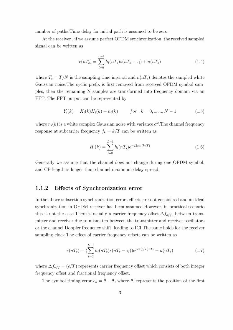
number of paths.Time delay for initial path is assumed to be zero.

At the receiver , if we assume perfect OFDM synchronization, the received sampled

signal can be written as

r(nTs) =L−1∑l=0

hl(nTs)s(nTs − τl) + n(nTs) (1.4)

where Ts = T/N is the sampling time interval and n(nTs) denotes the sampled white

Gaussian noise.The cyclic prefix is first removed from received OFDM symbol sam-

ples, then the remaining N samples are transformed into frequency domain via an

FFT. The FFT output can be represented by

Yi(k) = Xi(k)Hi(k) + ni(k) for k = 0, 1, ..., N − 1 (1.5)

where ni(k) is a white complex Gaussian noise with variance σ2.The channel frequency

response at subcarrier frequency fk = k/T can be written as

Hi(k) =L−1∑l=0

hl(nTs)e−j2πτl(k/T ) (1.6)

Generally we assume that the channel does not change during one OFDM symbol,

and CP length is longer than channel maximum delay spread.

1.1.2 Effects of Synchronization error

In the above subsection synchronization errors effects are not considered and an ideal

synchronization in OFDM receiver has been assumed.However, in practical scenario

this is not the case.There is usually a carrier frequency offset,∆foff , between trans-

mitter and receiver due to mismatch between the transmitter and receiver oscillators

or the channel Doppler frequency shift, leading to ICI.The same holds for the receiver

sampling clock.The effect of carrier frequency offsets can be written as

r(nTs) = (L−1∑l=0

hl(nTs)s(nTs − τl))ej2π(ε/T )nTs + n(nTs) (1.7)

where ∆foff = (ε/T ) represents carrier frequency offset which consists of both integer

frequency offset and fractional frequency offset.

The symbol timing error eθ = θ − θ0 where θ0 represents the position of the first

3

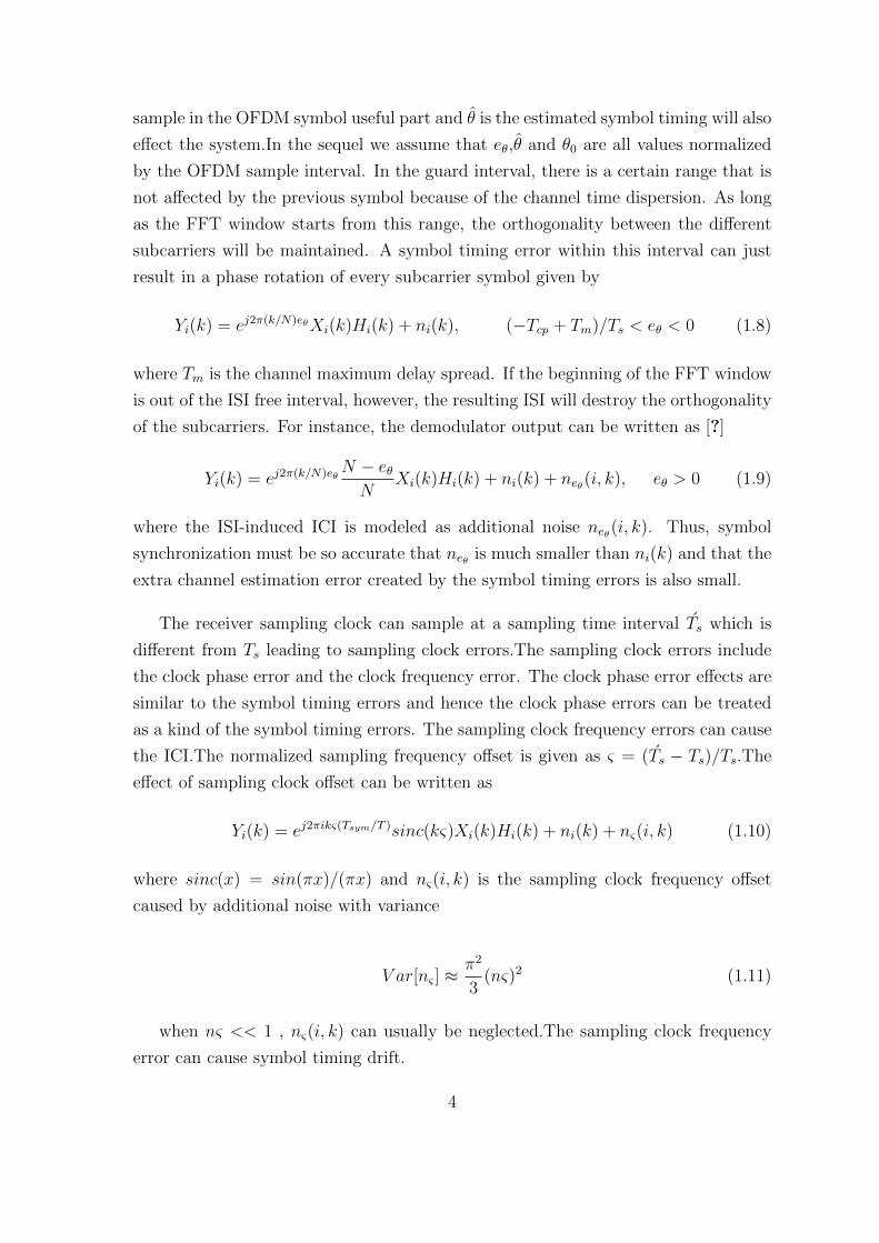
sample in the OFDM symbol useful part and θ is the estimated symbol timing will also

effect the system.In the sequel we assume that eθ,θ and θ0 are all values normalized

by the OFDM sample interval. In the guard interval, there is a certain range that is

not affected by the previous symbol because of the channel time dispersion. As long

as the FFT window starts from this range, the orthogonality between the different

subcarriers will be maintained. A symbol timing error within this interval can just

result in a phase rotation of every subcarrier symbol given by

Yi(k) = ej2π(k/N)eθXi(k)Hi(k) + ni(k), (−Tcp + Tm)/Ts < eθ < 0 (1.8)

where Tm is the channel maximum delay spread. If the beginning of the FFT window

is out of the ISI free interval, however, the resulting ISI will destroy the orthogonality

of the subcarriers. For instance, the demodulator output can be written as [?]

Yi(k) = ej2π(k/N)eθN − eθN

Xi(k)Hi(k) + ni(k) + neθ(i, k), eθ > 0 (1.9)

where the ISI-induced ICI is modeled as additional noise neθ(i, k). Thus, symbol

synchronization must be so accurate that neθ is much smaller than ni(k) and that the

extra channel estimation error created by the symbol timing errors is also small.

The receiver sampling clock can sample at a sampling time interval Ts which is

different from Ts leading to sampling clock errors.The sampling clock errors include

the clock phase error and the clock frequency error. The clock phase error effects are

similar to the symbol timing errors and hence the clock phase errors can be treated

as a kind of the symbol timing errors. The sampling clock frequency errors can cause

the ICI.The normalized sampling frequency offset is given as ς = (Ts − Ts)/Ts.The

effect of sampling clock offset can be written as

Yi(k) = ej2πikς(Tsym/T )sinc(kς)Xi(k)Hi(k) + ni(k) + nς(i, k) (1.10)

where sinc(x) = sin(πx)/(πx) and nς(i, k) is the sampling clock frequency offset

caused by additional noise with variance

V ar[nς ] ≈π2

3(nς)2 (1.11)

when nς << 1 , nς(i, k) can usually be neglected.The sampling clock frequency

error can cause symbol timing drift.

4

1.2 Cell Search and Synchronization

In the 3GPP LTE systems, the user equipment (UE) achieves time and frequency

synchronization with a cell and detects its cell identity in the procedure of cell search.

There are two kinds of cell search: initial cell search is performed when a UE is

switched on or when a UE loses its synchronization; neighbor cell search must be

performed periodically during idle and active modes to update the cell to be connected

and to find a candidate cell for handover.A two-step hierarchical neighbor cell search

process has been applied in the 3GPP LTE systems [?]. In this thesis a non-coherent

detection is performed for both PSS and SSS detection.

Firstly, the primary synchronization signal (PSS) is detected in time domain to

get the slot synchronization and sector identity (one among three sectors). Secondly,

frame synchronization and cell group identity (one among 168 groups) are obtained

by detecting the secondary synchronization signal (SSS) in frequency domain. In

addition to detecting symbol timing and physical layer ID(or sector-ID) from PSS in

time domain, fractional frequency offset is also estimated from PSS by making use of

CP based correlation approach [?]. In general, coherent detection is usually utilized

for SSS detection, where the channel response is estimated from primary synchro-

nization channel (PSCH) by the detected PSS [?]-[?]. However, owing to the limited

number of PSS, there may be more than one neighbor cell with the same PSS, and

the channel response estimated from PSCH could not exactly match the channel re-

sponse of the target cell. Moreover, the channel response differences between PSCH

and secondary synchronization channel (SSCH) will become obvious in high Doppler

frequency environment.Even in low Doppler frequency environment, in TDD mode,

performance degradation is occurred by difference of channel between PSS and SSS,

since PSS and SSS signals are separated by two OFDM symbols in TDD mode.To

solve this problem a non-coherent detection approach for SSS detection is followed in

this thesis, which has stable performance regardless of doppler frequency.In addition

to detecting radio frame timing and cell-ID, integer frequency offset is also estimated

using SSS signal in frequency domain.After cell search and correcting for synchro-

nization errors, channel estimation is performed on PSS and SSS data that include

both simulated data and real time captured data, using 1D-MMSE and subsequent

plots are generated.

Once UE detects the cell-ID and obtains downlink synchronization of the serving

cell(enodeB), UE needs to indicate its presence to the serving cell and also get up-

link synchronized with the serving cell.The propagation delay encountered by each

5

user for transmissions between eNodeB and UE is distance dependent.Different lo-

cation of UE in the cell causes unequal propagation delays, leading to misalignment

of symbols at the eNodeB, which may result in loss of uplink intra-cell orthogonal-

ity.Thus eNodeB needs to estimate propagation delays of different UE’s and corre-

spondingly adjust their transmission time instant so that all the UE’s gets uplink syn-

chronized with eNodeB.After initial cell search the UE decodes the information send

on the Physical Broadcast Channel(PBCH), which includes cell specific information

like Bandwidth,number of transmit antennas used by eNodeB etc.PBCH informa-

tion also includes parameters required by the UE to perform uplink synchronization,

which is initiated by UE by transmitting preamble to eNodeB on Physical Random

Access Channel(PRACH). In this thesis both full frequency domain and hybrid time-

frequency domain approach has been followed for PRACH preamble detection at

eNodeB.

This thesis is organized as follows.Chapter 2 describes about PSS and SSS sig-

nals structure and generation along with the system model and frame structures in

LTE.Chapter 3 describes sector and cell search along with detecting cell-ID and es-

timating symbol timing and frequency offsets based on proposed scheme.In Chapter

4 PRACH structure is discussed whereas in Chapter 5 practical implementation of

PRACH and its detection based on proposed method are discussed.Simulation re-

sults along with the results obtained by working on real time RF captured data are

presented in chapter 6. Finally conclusion and future work is presented in chapter 7.

6

Chapter 2

Downlink Synchronization signals

A UE wishing to access an LTE cell must first undertake a cell search procedure.

This consists of a series of synchronization stages by which the UE determines time

and frequency parameters that are necessary to demodulate the downlink and to

transmit uplink signals with the correct timing. The UE also acquires some critical

system parameters.Two major synchronization requirements can be identified in the

LTE system: the first is symbol timing acquisition, by which the correct symbol

start position is determined, for example to set the FFT window position;the second

is carrier frequency synchronization, which is required to reduce or eliminate the

effect of frequency errors arising from a mismatch of the local oscillators between the

transmitter and the receiver, as well as the Doppler shift caused by the UE motion.

Two relevant cell search procedures exist in LTE:the first is Initial syncroniza-

tion,where by the UE detects an LTE cell and decodes all the information required

to register to it. This would be required, for example, when the UE is switched on,

or when it has lost the connection to the serving cell;the second is the New cell iden-

tification, performed when a UE is already connected to an LTE cell and is in the

process of detecting a new neighbour cell. In this case, the UE reports to the serving

cell measurements related to the new cell, in preparation for handover. In both sce-

narios, the synchronization procedure makes use of two specially designed physical

signals which are broadcast in each cell: the Primary Synchronization Signal (PSS)

and the Secondary Synchronization Signal (SSS). The detection of these two signals

not only enables time and frequency synchronization, but also provides the UE with

the physical layer identity of the cell and the cyclic prefix length, and informs the

UE whether the cell uses Frequency Division Duplex (FDD) or Time Division Duplex

(TDD).

In the case of the initial synchronization, in addition to the detection of synchro-

7

Figure 2.1: PSS and SSS frame and slot structure in time domain in the FDD case.

nization signals, the UE proceeds to decode the Physical Broadcast CHannel (PBCH),

from which critical system information is obtained.In the case of new cell identifica-

tion, the UE does not need to decode the PBCH; it simply makes quality-level mea-

surements based on the reference signals transmitted from the newly-detected cell

and reports these to the serving cell.

The PSS and SSS structure in time is shown in Figure 2.1 for the FDD case

and in Figure 2.2 for TDD:the synchronization signals are transmitted periodically,

twice per 10 ms radio frame [?]. In an FDD cell, the PSS is always located in the

last OFDM (Orthogonal Frequency Division Multiplexing) symbol of the first and

11th slots of each radio frame, thus enabling UE to acquire the slot boundary timing

independently of the Cyclic Prefix (CP) length. The SSS is located in the symbol

immediately preceding the PSS, a design choice enabling coherent detection of the SSS

relative to the PSS, based on the assumption that the channel coherence duration is

significantly longer than one OFDM symbol. In a TDD cell, the PSS is located in the

third symbol of the 3rd and 13th slots, while the SSS is located three symbols earlier;

coherent detection can be used under the assumption that the channel coherence time

is significantly longer than four OFDM symbols.

In the frequency domain, the mapping of the PSS and SSS to subcarriers is shown

in Figure 2.3. The PSS and SSS are transmitted in the central six Resource Blocks

(RBs), enabling the frequency mapping of the synchronization signals to be invariant

8

Figure 2.2: PSS and SSS frame and slot structure in time domain in the TDD case.

with respect to the system bandwidth (which can vary from 6 to 110 RBs) ; this

allows the UE to synchronize to the network without any a priori knowledge of the

allocated bandwidth. The PSS and SSS are each comprised of a sequence of length

62 symbols,mapped to the central 62 subcarriers around the d.c. subcarrier which

is left unused. This means that the five resource elements at each extremity of each

synchronization sequence are not used.

The particular sequences which are transmitted for the PSS and SSS in a given

cell are used to indicate the physical-layer cell identity to the UE.There are 504

unique physical-layer cell identities. The physical-layer cell identities are grouped

into 168 unique physical-layer cell-identity groups, each group containing three unique

identities. The grouping is such that each physical-layer cell identity is part of one

and only one physical-layer cell-identity group. A physical-layer cell identity N cellID =

3N(1)ID + N

(2)ID is thus uniquely defined by a number N

(1)ID in the range of 0 to 167,

representing the physical-layer cell-identity group, and a number N(2)ID in the range of

0 to 2, representing the physical-layer identity within the physical-layer cell-identity

group.The three identities in a group would usually be assigned to cells under the

control of the same eNodeB.Three PSS sequences are used to indicate the cell identity

within the group, and 168 SSS sequences are used to indicate the identity of the group.

9

Figure 2.3: PSS and SSS frame structure in frequency and time domain for an FDDcell.

2.1 Primary synchronization Signal

Primary syncronization signal is constructed from one of the three length-63 Zadoff-

Chu sequence in the frequency domain, with the middle element puncutured to avoid

transmitting on d.c subcarrier.Three PSS sequences are used in LTE, corresponding

to the three physical layer identities(N(2)ID = 0, 1, 2) within each group of cells.

2.1.1 Sequence generation

The sequence d(n) used for the primary synchronization signal is generated from a

frequency-domain Zadoff-Chu sequence according to

du(n) = e−jun(n+1)

63 , n = 0, 1, . . . , 62. (2.1)

where the Zadoff-Chu root sequence index u is given by Table 3.1

This set of roots for the ZC sequences was chosen for its good periodic auto-

correlation and cross-correlation properties. In particular, these sequences have a

low-frequency offset sensitivity, defined as the ratio of the maximum undesired auto-

correlation peak in the time domain to the desired correlation peak computed at a

10

N(2)ID Root index u0 251 292 34

Table 2.1: Root indices for the primary synchronization signal.

certain frequency offset. This allows a certain robustness of the PSS detection during

the initial synchronization.

2.2 Secondary synchronization signal

The SSS consists of a frequency domain sequence, which is an interleaved concatena-

tion of two length-31 m-sequences, named as even sequence and odd sequence here.

Both even sequence and odd sequence are scrambled by an m-sequence whose cyclic

shift value is dependent on sector identity. The odd sequence is further scrambled by

an m-sequence with cyclic shift value determined by even sequence. The combina-

tion of cyclic shifts of even sequence and odd sequence corresponds to the cell group

identity. These two length-31 sequences differ every 5ms, which allows UE to detect

the 10ms frame timing.

2.2.1 Sequence generation

The sequence d(0),...,d(61) used for the second synchronization signal is an inter-

leaved concatenation of two length-31 binary sequences. The concatenated sequence

is scrambled with a scrambling sequence given by the primary synchronization sig-

nal.The combination of two length-31 sequences defining the secondary synchroniza-

tion signal differs between subframe 0 and subframe 5 according to

d(2n) =

{s

(m0)0 (n)c0(n) in subframe 0

s(m1)1 (n)c0(n) in subframe 5

(2.2)

d(2n+ 1) =

{s

(m1)1 (n)c1(n)z

(m0)1 (n) in subframe 0

s(m0)0 (n)c1(n)z

(m1)1 (n) in subframe 5

(2.3)

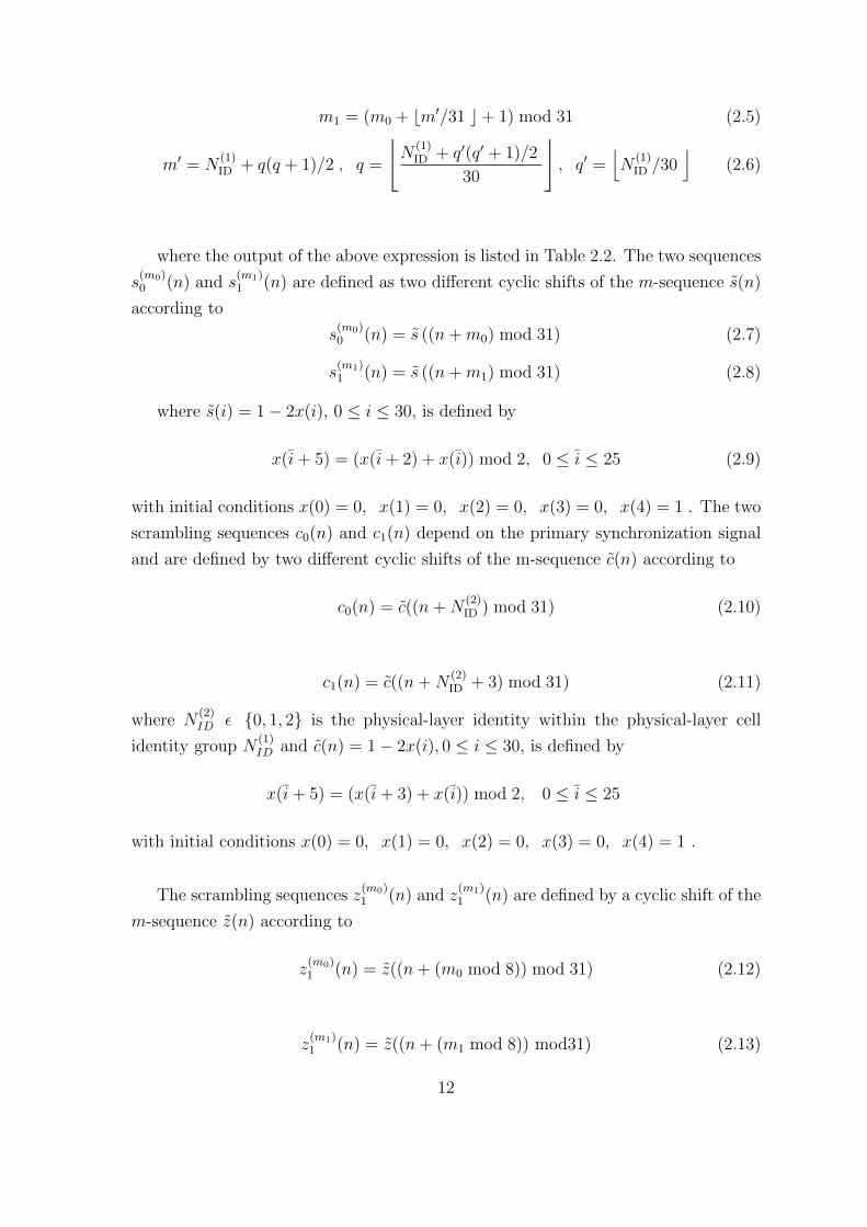
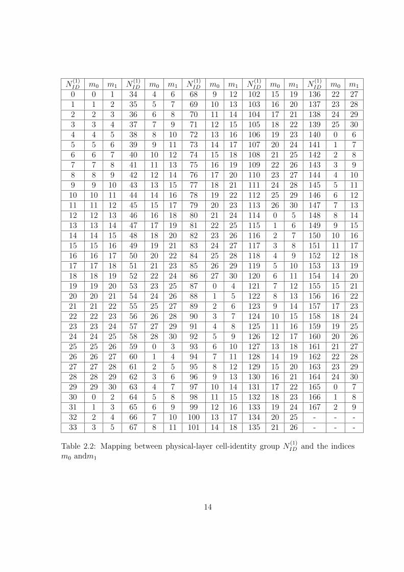
where 0 ≤ n ≤ 30 . The indices m0 and m1 are derived from the physical-layer

cell-identity group N(1)ID according to

m0 = m′ mod 31 (2.4)

11

m1 = (m0 + bm′/31 c+ 1) mod 31 (2.5)

m′ = N(1)ID + q(q + 1)/2 , q =

⌊N

(1)ID + q′(q′ + 1)/2

30

⌋, q′ =

⌊N

(1)ID /30

⌋(2.6)

where the output of the above expression is listed in Table 2.2. The two sequences

s(m0)0 (n) and s

(m1)1 (n) are defined as two different cyclic shifts of the m-sequence s(n)

according to

s(m0)0 (n) = s ((n+m0) mod 31) (2.7)

s(m1)1 (n) = s ((n+m1) mod 31) (2.8)

where s(i) = 1− 2x(i), 0 ≤ i ≤ 30, is defined by

x(i+ 5) = (x(i+ 2) + x(i)) mod 2, 0 ≤ i ≤ 25 (2.9)

with initial conditions x(0) = 0, x(1) = 0, x(2) = 0, x(3) = 0, x(4) = 1 . The two

scrambling sequences c0(n) and c1(n) depend on the primary synchronization signal

and are defined by two different cyclic shifts of the m-sequence c(n) according to

c0(n) = c((n+N(2)ID ) mod 31) (2.10)

c1(n) = c((n+N(2)ID + 3) mod 31) (2.11)

where N(2)ID ε {0, 1, 2} is the physical-layer identity within the physical-layer cell

identity group N(1)ID and c(n) = 1− 2x(i), 0 ≤ i ≤ 30, is defined by

x(i+ 5) = (x(i+ 3) + x(i)) mod 2, 0 ≤ i ≤ 25

with initial conditions x(0) = 0, x(1) = 0, x(2) = 0, x(3) = 0, x(4) = 1 .

The scrambling sequences z(m0)1 (n) and z

(m1)1 (n) are defined by a cyclic shift of the

m-sequence z(n) according to

z(m0)1 (n) = z((n+ (m0 mod 8)) mod 31) (2.12)

z(m1)1 (n) = z((n+ (m1 mod 8)) mod31) (2.13)

12

where m0 and m1 are obtained from Table 2.2 and z(i) = 1 − 2x(i), 0 ≤ i ≤ 30, is

defined by

x(i+ 5) = (x(i+ 4) + x(i+ 2) + x(i+ 1) + x(i)) mod2, 0 ≤ i ≤ 25

with initial conditions x(0) = 0, x(1) = 0, x(2) = 0, x(3) = 0, x(4) = 1 .

13

N(1)ID m0 m1 N

(1)ID m0 m1 N

(1)ID m0 m1 N

(1)ID m0 m1 N

(1)ID m0 m1

0 0 1 34 4 6 68 9 12 102 15 19 136 22 271 1 2 35 5 7 69 10 13 103 16 20 137 23 282 2 3 36 6 8 70 11 14 104 17 21 138 24 293 3 4 37 7 9 71 12 15 105 18 22 139 25 304 4 5 38 8 10 72 13 16 106 19 23 140 0 65 5 6 39 9 11 73 14 17 107 20 24 141 1 76 6 7 40 10 12 74 15 18 108 21 25 142 2 87 7 8 41 11 13 75 16 19 109 22 26 143 3 98 8 9 42 12 14 76 17 20 110 23 27 144 4 109 9 10 43 13 15 77 18 21 111 24 28 145 5 1110 10 11 44 14 16 78 19 22 112 25 29 146 6 1211 11 12 45 15 17 79 20 23 113 26 30 147 7 1312 12 13 46 16 18 80 21 24 114 0 5 148 8 1413 13 14 47 17 19 81 22 25 115 1 6 149 9 1514 14 15 48 18 20 82 23 26 116 2 7 150 10 1615 15 16 49 19 21 83 24 27 117 3 8 151 11 1716 16 17 50 20 22 84 25 28 118 4 9 152 12 1817 17 18 51 21 23 85 26 29 119 5 10 153 13 1918 18 19 52 22 24 86 27 30 120 6 11 154 14 2019 19 20 53 23 25 87 0 4 121 7 12 155 15 2120 20 21 54 24 26 88 1 5 122 8 13 156 16 2221 21 22 55 25 27 89 2 6 123 9 14 157 17 2322 22 23 56 26 28 90 3 7 124 10 15 158 18 2423 23 24 57 27 29 91 4 8 125 11 16 159 19 2524 24 25 58 28 30 92 5 9 126 12 17 160 20 2625 25 26 59 0 3 93 6 10 127 13 18 161 21 2726 26 27 60 1 4 94 7 11 128 14 19 162 22 2827 27 28 61 2 5 95 8 12 129 15 20 163 23 2928 28 29 62 3 6 96 9 13 130 16 21 164 24 3029 29 30 63 4 7 97 10 14 131 17 22 165 0 730 0 2 64 5 8 98 11 15 132 18 23 166 1 831 1 3 65 6 9 99 12 16 133 19 24 167 2 932 2 4 66 7 10 100 13 17 134 20 25 - - -33 3 5 67 8 11 101 14 18 135 21 26 - - -

Table 2.2: Mapping between physical-layer cell-identity group N(1)ID and the indices

m0 andm1

14

Chapter 3

Decoding downlink

synchronization signal

3.1 System model

We consider the transmission of a serial discrete baseband OFDM stream s(n) given

by

s(n) =1√N

N−1∑k=0

Xkej2πkn/N , 1 ≤ n ≤ N (3.1)

where Xk denotes the modulated data on the kth sub-carrier and N the FFT

size.Transmitting over a multipath propagation channel under consideration of a fre-

quency misalignment between transmitter and receiver oscillators as well as additive

white Gaussian noise (AWGN), the received signal will be

r(n) = [s(n) ⊗ h(n)] ej2πεn/N + w(n) , (3.2)

where h(n) represents channel impulse response (CIR), ε denotes the frequency mis-

match with respect to the sub-carrier spacing, w(n) is the noise term and ⊗ stands

for circular convolution.The CIR is modeled as

h(n) =

Nd−1∑d=0

hdδ(n− d) (3.3)

where Nd is the number of channel taps and hd the complex value of the d-th Rayleigh-

distributed tap.The mean power of hd follows an exponential decay and is given by

15

σ2d = e

−dτ , (3.4)

where τ is the power decay constant.

After applying the N -point FFT at the receiver and assuming perfect timing, the

OFDM symbol is given by

Yl =1√N

N−1∑n=0

r(n)e−j2πln/N =1

N

N−1∑k=0

HkXk

N−1∑n=0

e2π(k−l+ε)/N +Wk (3.5)

with

Hk =N−1∑l=0

hle−j2πkl/N andWk =

1√N

N−1∑n=0

w(n)e−j2πnk/N (3.6)

As it can be observed from Equation (4.5) , the received OFDM symbol will be

affected not only by the channel and noise distortions Hk and Wk , but also by a

term due to CFO(ε). The received OFDM symbol Yl constellation will be rotated by

an equal phase known as the common phase error(CPE) ,which is independent of the

particular sub-carrier.Furthermore, the loss of orthogonality between sub-carrier has

a noise-like effect called inter-carrier-interference(ICI).

3.2 Time and frequency synchronization

The objective of synchronization is to retrieve OFDM symbol timing and to estimate

the carrier frequency offset (CFO). The CFO can be separated into an integer part,

which is a multiple of the sub-carrier spacing, and a fractional part, which is respon-

sible for the CPE and ICI. The CFO regarding the sub-carrier spacing can be thus

given as

ε = nI + εF ,

where nI is the integer number of sub-carrier spacing and εF the fractional part

with −1 < ε < 1. In [?] we investigated several approaches on time and frequency

synchronization for LTE. According to conclusions of this study, we decide to use the

cyclic prefix based method for acquisition of the OFDM symbol timing and fractional

CFO, as it is originally proposed in [?]. The log-likelihood function for the OFDM

symbol start (θ) and the frequency mismatch (εF ) can be written as

16

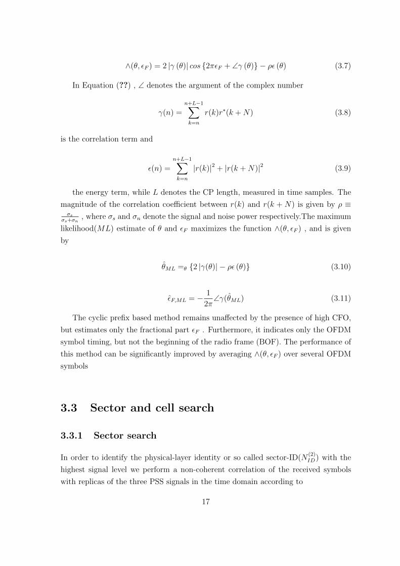
∧(θ, εF ) = 2 |γ (θ)| cos {2πεF + ∠γ (θ)} − ρε (θ) (3.7)

In Equation (??) , ∠ denotes the argument of the complex number

γ(n) =n+L−1∑k=n

r(k)r∗(k +N) (3.8)

is the correlation term and

ε(n) =n+L−1∑k=n

|r(k)|2 + |r(k +N)|2 (3.9)

the energy term, while L denotes the CP length, measured in time samples. The

magnitude of the correlation coefficient between r(k) and r(k + N) is given by ρ ≡σs

σs+σn, where σs and σn denote the signal and noise power respectively.The maximum

likelihood(ML) estimate of θ and εF maximizes the function ∧(θ, εF ) , and is given

by

θML =θ {2 |γ(θ)| − ρε (θ)} (3.10)

εF,ML = − 1

2π∠γ(θML) (3.11)

The cyclic prefix based method remains unaffected by the presence of high CFO,

but estimates only the fractional part εF . Furthermore, it indicates only the OFDM

symbol timing, but not the beginning of the radio frame (BOF). The performance of

this method can be significantly improved by averaging ∧(θ, εF ) over several OFDM

symbols

3.3 Sector and cell search

3.3.1 Sector search

In order to identify the physical-layer identity or so called sector-ID(N(2)ID) with the

highest signal level we perform a non-coherent correlation of the received symbols

with replicas of the three PSS signals in the time domain according to

17

Qi(n) =i

N−1∑k=0

d∗i (k)r(n+ k), (3.12)

where di(k) denotes the replica of ith PSS sequence, N is the PSS time domain signal

length, k is the time domain index and r(k) the received symbols.The magnitude of the

non-coherent correlator output |Qi(n)| corresponding to the sector with the highest

signal shows a large peak compared to the other correlation terms due to orthogonality

between sequences.Thus, the estimated physical-layer identity or sector-ID(N(2)ID) is

given by

Ns =i (|Qi(n)|) (3.13)

Simultaneously, the approximate position of the start of the PSS sequence from

the received signal is given by

mNs=n

(∣∣QNs(n)∣∣) (3.14)

The maximum likelihood (ML) estimate of the start of the PSS symbol and also

the fractional frequency offset can be found out by Cyclic prefix correlation based

on Equations (??) and (??) respectively.Simultaneously, the sector identification in-

dicates the radio frame start as the PSS sequence position within the radio frame is

already known, however with an uncertainty between first and sixth sub-frame. This

information is retrieved by decoding the SSS signal, as explained in following Section

(??)

3.4 Cell-ID search and Integer carrier frequency

offset estimation

The cell-ID needs to be estimated correctly, in order to establish connection with the

best possible serving base station.The group-ID N(1)ID can be jointly estimated with the

integer Carrier Frequency Offset(CFO) nI and the sub-frame index within the radio

frame(0 or 5). The basic concept is to exploit the cyclic shifts of the two length-31

binary sequences s(m0)0 (n) and s

(m1)1 (n) according to the pair of integers m0 and m1,

which identify the group-ID. The quantity of integer CFO nI can be estimated by the

sub-carrier shift of the frequency domain SSS sequence d(n). The method proposed

here consists of following steps:

18

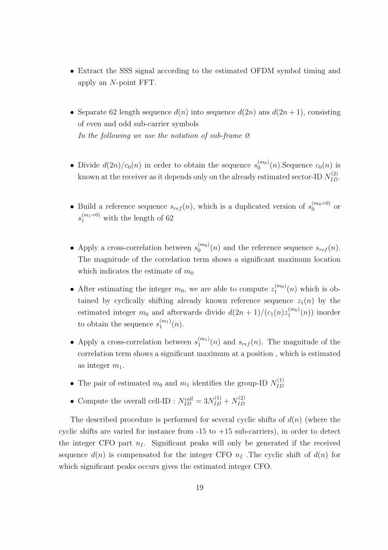
• Extract the SSS signal according to the estimated OFDM symbol timing and

apply an N -point FFT.

• Separate 62 length sequence d(n) into sequence d(2n) ans d(2n+ 1), consisting

of even and odd sub-carrier symbols

In the following we use the notation of sub-frame 0:

• Divide d(2n)/c0(n) in order to obtain the sequence s(m0)0 (n).Sequence c0(n) is

known at the receiver as it depends only on the already estimated sector-IDN(2)ID .

• Build a reference sequence sref (n), which is a duplicated version of s(m0=0)0 or

s(m1=0)1 with the length of 62

• Apply a cross-correlation between s(m0)0 (n) and the reference sequence sref (n).

The magnitude of the correlation term shows a significant maximum location

which indicates the estimate of m0

• After estimating the integer m0, we are able to compute z(m0)1 (n) which is ob-

tained by cyclically shifting already known reference sequence z1(n) by the

estimated integer m0 and afterwards divide d(2n + 1)/(c1(n)z(m0)1 (n)) inorder

to obtain the sequence s(m1)1 (n).

• Apply a cross-correlation between s(m1)1 (n) and sref (n). The magnitude of the

correlation term shows a significant maximum at a position , which is estimated

as integer m1.

• The pair of estimated m0 and m1 identifies the group-ID N(1)ID

• Compute the overall cell-ID : N cellID = 3N

(1)ID +N

(2)ID

The described procedure is performed for several cyclic shifts of d(n) (where the

cyclic shifts are varied for instance from -15 to +15 sub-carriers), in order to detect

the integer CFO part nI . Significant peaks will only be generated if the received

sequence d(n) is compensated for the integer CFO nI .The cyclic shift of d(n) for

which significant peaks occurs gives the estimated integer CFO.

19

Chapter 4

Uplink Synchronizations

Random access channel is an uplink channel which acts as an interface between non-

synchronized UE’s and the orthogonal transmission scheme of the LTE uplink radio

access, unless and until a UE is uplink synchronized any uplink transmission is not

possible. Physical Random Access Channel (PRACH) is the physical layer equivalent

of a Random access channel (RACH), i.e it defines the time-frequency resource on

which RACH preamble is actually transmitted.

4.1 Initial access

Before the user equipment can start transmitting and receiving data it must connect

to the network. This connection phase consists of 3 stages where UE (Terminal)

extracts some set of information in each stage. The three stages that each UE should

undergo before any transmission or reception are given below. This combined process

is known as LTE initial access

4.1.1 Cell search

The first thing that happens in the access procedure is that the UE gets identified

within the network. This procedure is called the cell search, which includes in estab-

lishment of synchronization between UE and the cell and acquiring the information

about cell. The synchronization procedures are performed in order to obtain timing

synchronization for correct symbol detection and also for frequency synchronization

to annihilate frequency mismatches caused by movement of UE or different oscilla-

tors at the receiving and transmitting sides.The downlink synchronization is achieved

by receiving primary and secondary synchronization sequences, details of which are

20

explained in chapter 2 and 3.

4.1.2 Derive system information

The second part of the access procedure is where the UE needs to derive system

information. This system information is periodically broadcasted in the network and

this information is needed for the UE to be able to connect to the network and a

specific cell within that network. When the UE has received and decoded the system

information it has information about for example cell bandwidths and parameters

specific to random access.

4.1.3 Random access

Random access is used to achieve uplink time synchronization for a UE which either

has not yet acquired, or has lost its uplink synchronization. Once uplink synchroniza-

tion is achieved for a UE, the eNodeB can schedule orthogonal uplink transmission

resources for it.Random access is generally performed when the UE turns on from

sleep mode, performs handoff from one cell to another or when it loses uplink timing

synchronization.Random access is generally performed when the UE turns on from

sleep mode, performs handoff from one cell to another or when it loses uplink tim-

ing synchronization.Random access allows the eNodeB to estimate and, if needed,

adjust the UE uplink transmission timing to within a fraction of the cyclic prefix.

When an eNodeB successfully receives a random access preamble, it sends a ran-

dom access response indicating the successfully received preamble(s) along with the

timing advance (TA) and uplink resource allocation information to the UE. The UE

can then checks if its random access attempt has been successful by matching the

preamble number it used for random access with the preamble number information

received from the eNodeB. If the preamble number matches, the UE concludes that

its preamble transmission attempt has been successful and it then adjust its uplink

timing based on the Timing Advance(T.A) that it has received. If the preamble num-

ber does not match then it tries for retransmission.After the UE has acquired uplink

timing synchronization, it can transmit data in uplink.

4.1.4 Timing correction

The propagation delay encountered by each user for transmissions between eNodeB

and UE is distance dependent i.e, user very close to base station encounters less

21

delay compared to cell edge user.If suppose the near by user and cell edge user are

allocated with same uplink time resource but different frequency resources (Resource

blocks) then because of inequal propagation delays in their transmissions on uplink

the reception of both users at eNodeB may not be alligned properly which may result

in loss of uplink intra-cell orthogonality, in contrary if both users are allocated with

same frequency resource but different time instants there is every possibility that the

transmission of one user may get smeared into the transmission of next user (with

an assumption that preceding used is cell edge user) which may lead to inter symbol

interference.

In order to avoid timing misalignment of different users at eNodeB , if eNodeB

could able to calculate their propagation delays apriorly by some means and instruct

each user to correct its timing before transmission of any data on uplink then all

UE transmissions can be perfectly aligned at eNodeB. The Random access process

helps eNodeB in figuring out the propagation delays of each UE,eNodeB calculates the

propagation delays of all UEs from their preamble transmissions on PRACH and then

instructs corresponding UE to correct its timing of transmission,i.e either advance in

time or retard in time,i.e upon receiving this command cell edge user will advance his

transmission by the amount specified by the eNodeB,i.e if cell edge user is allotted

a time slot t for its transmission and if it is instructed to advance by t1 seconds to

counter its propagation delay then instead of transmitting at tth interval the cell edge

user start transmitting before tth i.e at (t− t1)th instant.

4.2 Random Access Procedure

A downlink synchronized UE which needs to achieve uplink synchronization will trans-

mit a random access preamble (signature) on uplink on time-frequency resources as

specified by the system. Each cell comprise of 64 random access preambles and UE

which requires uplink synchronization randomly selects one of the preamble and trans-

mit it on uplink PRACH. When a UE transmit a PRACH Preamble, it transmits with

a specific pattern and this specific pattern is called a ”Signature”.

The random access process occurs in two forms in LTE, which indicate either

contention-based(possibility of collision) or contention-free.In the case of contention-

based random access procedure each UE randomly selects one among the available

random access preamble signature, with a possibility for more than one UE simulta-

neously to transmit the same preamble signature, which needs a contention resolution

procedure.On the other hand if a UE needs to perform a handover,where UE is al-

22

ready in connection mode, the eNodeB allocates dedicated signatures to UE from the

group of signatures which are exclusively allotted for contention-free purpose.Thus

the contention-free random access procedure has no possibility of collision, leading to

a faster random access procedure, which is crucial in case of handover.

A cell has a fixed number 64 of preamble signatures, and these signatures are par-

titioned between those for contention-based access and those reserved for allocation

to specific UE’s on a contention-free basis. The two procedures are outlined in the

following sections.

4.2.1 Contention-based Random Access Procedure

The contention-based procedure is a four step process,as shown in Figure ??

Figure 4.1: Contention-based Random Access Procedure

Step 1: Transmission of Random Access Preamble:

The UE randomly picks one of the contention based preamble signature and trans-

mit it on PRACH allowing the eNodeB to estimate the transmission timing of the

terminal. Preamble signatures allocated for contention-based procedure are further

divided into two groups based on the size of transmission resource needed by UE

23

for step 3, which include small transmission resource demanding preambles and large

transmission resource demanding preambles. The purpose behind this division is if

suppose the message to be transmitted at step 3 is of small size and eNodeB has allot-

ted more resources for subsequent transmission then it may lead to inefficient usage

of uplink time-frequency resources. Based on transmission resource needed for trans-

mission of data in step 3 UE selects randomly one preamble among the two subgroups

of contention based preambles and transmit that preamble on the radio resources as

allocated by the eNodeB.The eNodeB can control the number of preamble signatures

in each group based on the observed loads.The initial preamble transmission power

setting is based on an open -loop estimation with full compensation for the path-loss.

This is designed to ensure that the received power of the preambles is independent

of the path-loss; this is designed to help the eNodeB to detect several simultaneous

preamble transmissions in the same time-frequency PRACH resource. The UE es-

timates the path-loss by averaging measurements of the downlink Reference Signal

Received Power (RSRP). The radio resources on which RACH process should occur

will be configured by eNodeB and propagated through broad cast channel as a part

of system information

Step 2: Random access response:

In response to the transmitted preamble, eNodeB transmits a random access re-

sponse(RAR) on physical downlink shared channel which contains • Random Access

Radio Network Temporary Identifier (RA-RNTI)

• Timing alignment command

• Initial uplink resource grant for transmission of the message in step 3

• Temporary Cell Radio Network Temporary Identifier (C-RNTI).

Random Access Radio Network Temporary Identifier (RA-RNTI) :It

identifies which time-frequency resources are utilized by the UE to transmit the Ran-

dom Access Preamble i.e the time-frequency slot in which the preamble was trans-

mitted , the RA-RNTI is essentially the sub frame number in which the UE has

transmitted which gets added by 1 .After UE transmits its preamble, it waits for a

RAR (random access response) associated with its implicit RA-RNTI to see if the

eNodeB heard the preamble. If it finds a suitable RAR, then it looks to see if its spe-

cific preamble sequence is included; if so, then the UE assumes it received a positive

24

acknowledge from the eNodeB and proceeds with subsequent steps.

The RA-RNTI is determined from the UE’s preamble transmission; the tempo-

rary C-RNTI is assigned by the eNodeB. Any UE sending a preamble in subframe

n will look for a response with an RA-RNTI with value n + 1; it then has to parse

the response to see if there’s a specific RAR in the response corresponding to the

preamble the UE used. Up to 64 UEs can send a preamble in the same subframe, and

still be distinguished (assuming they manage to pick a unique preamble). If multiple

UEs has transmitted the same preamble on same time-frequency resources all of them

obviously receive the same RA-RNTI.

Timing alignment command: Based on the propagation delay associated with

each UE transmission (measured from Transmitted preamble), the network deter-

mines the required timing correction for each UE. If the timing of a specific terminal

needs correction, the network issues a timing advance command for this specific ter-

minal, instructing it to retard or advance its timing relative to the current uplink

timing, and this command is very much necessary in order to maintain synchroniza-

tion among multiple UE uplink transmissions.

Initial uplink resource grant for transmission of the message:This spec-

ifies the amount of resource allocated by eNodeB for step 3 message transmission

.It includes a 10 bit fixed size resource block, and type of modulation and coding

scheme to be employed which will be indicated via a 4 bit string and transmission

power control command indicated by 3 bit string, uplink delay and CQI request each

indicated by one bit.

Temporary Cell Radio Network Temporary Identifier:TC-RNTI is a tem-

porary identifier assigned by the eNodeB to UE by means of which UE can perform

subsequent signaling to the eNodeB. C-RNTI is used by a given UE while it is in

a particular cell ,where the UE is already in connected mode. If no prior allotted

C-RNTI is available with UE then it uses temporary RNTI for further communica-

tion between the UE and eNodeB, if communication is successful then TC-RNTI is

promoted to C-RNTI.

The UE expects to receive the RAR within a time window, of which the start and

end are configured by the eNodeB and broadcast as part of the cell-specific system

information. The earliest subframe allowed by the specifications occurs 2 ms after

the end of the preamble sub frame. However, a typical delay (measured from the

25

end of the preamble subframe to the beginning of the first subframe of RAR win-

dow) is more likely to be 4 ms. If the UE is unable to receive the RAR within the

specified RAR slot as configured by eNodeB then the UE needs to retransmit the

preamble after some backoff time and this backoff-time, which specifies the time UE

need to wait after RAR window to retransmit the preamble is configured by eNodeB.

Every retransmission comes with increase in transmission power,UE retransmits the

preamble with slightly higher power compared to original transmission and the in-

crease of power in each retransmission is known as power ramping and is configured

by eNodeB as power-ramping-step. The UE need to stop transmitting preamble after

some successive trails, the number of retransmission that UE should undergo is also

configured by eNodeB.

Step 3: Message on UL-SCH:

The uplink of the UE terminal will get time synchronized after receiving the RAR.

However, before user data can be transmitted to/from the terminal, a unique identity

within the cell, the C-RNTI, must be assigned to the terminal. Depending on the

terminal (UE) state, there may also be a need for additional message exchange for

setting up the connection. In the third step, the terminal transmits the necessary

messages to the eNodeB using the UL-SCH resources assigned in the random-access

response in the second step

Once UE receives Random access response and successfully decodes it and ex-

tracts the provided uplink grant and C-RNTI (TC-RNTI in case of initial access),

UE starts transmitting the layer2/layer3 message on specified uplink resource ,this

transmission may be a request for RRC connection establishment, tracking area up-

dates or scheduling request etc. If suppose more than one user has transmitted the

same preamble on same time-frequency resource in step 1 then all of those UE’s re-

ceive the same RAR allocating same time-frequency resource and same TC-RNTI

and all these users in contention will transmit their corresponding L2/L3 messages

on same time-frequency resource which may lead to one of the two possibilities One

possibility is that these multiple signals act as interference to each other and eNodeB

decodes neither of them in this case, none of the UE would have any response (HARQ

ACK) from eNodeB and they all think that RACH process has failed and go back

to step 1. The other possibility would be that eNodeB could successfully decode the

message from only one UE and failed to decode it from the other UE in this case,

the UE with the successful L2/L3 decoding on eNodeB side will get the HARQ ACK

from eNodeB.

26

Step 4: Contention resolution:

The Hybrid Automatic Repeat Request Acknowledgment process (HARQ) for step 3

message is called ”contention resolution” process. Contention resolution message is

addressed to C-RNTI (in case of RRC-Connected) or to temporary C-RNTI . Upon

reception of contention resolution message any one of the three possibilities may hap-

pen at UE

• The UE correctly decodes the message and detects its own identity: it sends back

a Positive Acknowledgment, ACK.

• The UE correctly decodes the message and discovers that it contains another

UEs identity (contention resolution) it sends nothing back (Discontinuous Trans-

mission,DTX).

• The UE fails to decode the message or misses the DL grant: it sends nothing

back(’DTX’).

4.2.2 Contention free random access

Figure 4.2: Contention-free Random Access Procedure

27

Each UE is assigned with a dedicated preamble signature in the case of Contention-

free random access, leaving no scope for contention.This contention-free random ac-

cess is extremely useful where low latency is required,such as handover and resumption

of downlink traffic for a UE. Contention free random access is a two step process as

shown in Figure ??

Preamble transmission and RAR are similar to that of contention based pro-

cess except that a dedicated preamble is transmitted where as in contention based

a randomly selected preamble was transmitted, since there is hardly any chance for

contention in this process message on uplink granted resource and contention resolu-

tion steps are not required.

4.3 PRACH resource requirements

4.3.1 Time resource

The time resource allocated for preamble transmission depends on the time duration

of the preamble to be transmitted, which varies with radius of cell in which UE is

located.Based on radius of cell to cover four different preamble formats are defined,

each having varying lengths of cyclic prefix and preamble lengths. A preamble slot

in time domain consists of 3 parts,which include Preamble sequence,Cyclic prefix

and Guard period.To account for the timing uncertainty and to avoid interference

with subsequent subframes which are not used for Random access (may be used

by PUSCH for data transmission), a guard time is used as part of the preamble

transmission. Before the start of random access UE has however achieved downlink

synchronization but yet to achieve uplink synchronization and hence there is a definite

timing uncertainty associated with each UE’s uplink transmission as the location of

the terminal in the cell is not known and this uncertainty is proportional to the cell

size and amounts to 6.7µs/km and thats why a guard period is appended in PRACH

slot as a part of preamble transmission. The use of cyclic prefix in PRACH preamble

transmission allows for frequency domain processing at the base station and also it

may even be used to absorb Inter Symbol Interference in case of large cell where delay

spread may extend guard period.

The minimum time duration configured for each RACH slot is 1ms. RACH trans-

mission is actually multiplexed with physical uplink shared channel transmission

(PUSCH), there is no separate resource for RACH transmission. Depending upon

28

the radius of cell to cover different preamble formats are configured by eNodeB for

subsequent transmission on RACH, preamble formats occupies a time duration of 1ms

to 3ms depending upon their preamble and cyclic-prefix lengths. The basic random

access sequence is of 1ms which can be employed to cover a cell of radius less than

15 km However in order to accommodate the cyclic prefix and guard time the actual

preamble sequence is shortened and is less than 1ms.

4.3.2 Sequence duration

The length of preamble sequence should be chosen with care and is driven by some

factors which are listed below

• Trade-off between sequence length and overhead: A single sequence must be as

long as possible to maximize the number of orthogonal preambles while still fitting

within a single subframe in order to keep the PRACH overhead small in most deploy-

ments,i.e selected sequence should be such that the cyclic shifts of sequence which

results in other orthogonal preambles should account for total preamble sequences

available with cell(64);

• Compatibility with the maximum expected round-trip delay;

• Compatibility between PRACH and PUSCH subcarrier spacings;

• Coverage performance

Constraint 1: The sequence length, Tseq should be more than 683.33µs.

Since the purpose of preamble transmission is to achieve uplink synchronization, which

includes estimation of propagation delay of user uplink transmission and issuing an ap-

propriate timing correction command, and hence length of preamble sequence should

account for round-trip time delay for a UE located at the edge of the largest expected

cell (100 km radius), including the maximum delay spread expected in such large

cells(Typically 16.67µs).

Tseq ≥ ((100× 2× 103)/(3× 108)) + (16.67× 10−6)s = 683.33µs.

Constraint 2: The length of preamble sequence should be integer multiple of

normal OFDM symbol duration (because PUSCH transmission is based on OFDM)

Since RACH transmission is multiplexed with PUSCH transmission it is desirable to

minimize the orthogonality loss in the frequency domain between the preamble sub-

carriers and the subcarriers of the surrounding uplink data transmissions on PUSCH.

This is achieved if the PUSCH data symbol subcarrier spacing ∆f is an integer mul-

29

tiple of the PRACH subcarrier spacing ∆fRA:

TSEQ = k × TSYM = k/∆f, k ∈ N

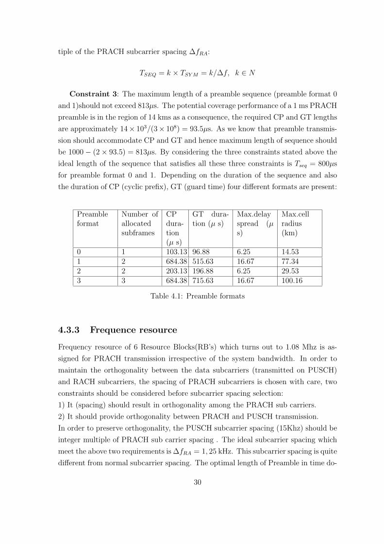
Constraint 3: The maximum length of a preamble sequence (preamble format 0

and 1)should not exceed 813µs. The potential coverage performance of a 1 ms PRACH

preamble is in the region of 14 kms as a consequence, the required CP and GT lengths

are approximately 14× 103/(3× 108) = 93.5µs. As we know that preamble transmis-

sion should accommodate CP and GT and hence maximum length of sequence should

be 1000− (2× 93.5) = 813µs. By considering the three constraints stated above the

ideal length of the sequence that satisfies all these three constraints is Tseq = 800µs

for preamble format 0 and 1. Depending on the duration of the sequence and also

the duration of CP (cyclic prefix), GT (guard time) four different formats are present:

Preambleformat

Number ofallocatedsubframes

CPdura-tion(µ s)

GT dura-tion (µ s)

Max.delayspread (µs)

Max.cellradius(km)

0 1 103.13 96.88 6.25 14.531 2 684.38 515.63 16.67 77.342 2 203.13 196.88 6.25 29.533 3 684.38 715.63 16.67 100.16

Table 4.1: Preamble formats

4.3.3 Frequence resource

Frequency resource of 6 Resource Blocks(RB’s) which turns out to 1.08 Mhz is as-

signed for PRACH transmission irrespective of the system bandwidth. In order to

maintain the orthogonality between the data subcarriers (transmitted on PUSCH)

and RACH subcarriers, the spacing of PRACH subcarriers is chosen with care, two

constraints should be considered before subcarrier spacing selection:

1) It (spacing) should result in orthogonality among the PRACH sub carriers.

2) It should provide orthogonality between PRACH and PUSCH transmission.

In order to preserve orthogonality, the PUSCH subcarrier spacing (15Khz) should be

integer multiple of PRACH sub carrier spacing . The ideal subcarrier spacing which

meet the above two requirements is ∆fRA = 1, 25 kHz. This subcarrier spacing is quite

different from normal subcarrier spacing. The optimal length of Preamble in time do-

30

main is 800µs and corresponding length in frequency domain is 1080/1.25 = 864 sub

carriers.

4.4 Resource allocation for PRACH

The resource allocated for PRACH will be different for FDD mode and TDD mode.The

following section describes the frame structure in LTE and PRACH resource allocation

for Frame structure type1(applicable for FDD) and Frame structure type2(applicable

for TDD).

Downlink and uplink transmissions are organized into radio frames with Tf =

307200 × Ts = 10ms duration, where Ts = 1/(15000 × 2048)s is the sampling time

duration.Two radio frame structure are supported in LTE, described in the following

sections

4.4.1 PRACH resources for frame structure type 1:

Each radio frame defined in LTE is Tf = 307200 × Ts = 10ms long and consists

of 20 slots of length Tslot = 15360 × Ts = 0.5ms, numbered from 0 to 19.Each

subframe consists of two consecutive slots.In case of FDD 10 subframes are available

for downlink transmission and 10 subframes are available for uplink transmissions in

each 10 ms interval. Uplink and downlink transmissions are separated in the frequency

domain. In half-duplex FDD operation, the UE cannot transmit and receive at the

same time while there are no such restrictions in full-duplex FDD.

For frame structure type 1 with preamble format 0− 3, there is at most one ran-

dom access resource per subframe. Table-?? lists the Frame structure type 1 random

access configuration for preamble format 0−3 and the subframes in which random ac-

cess preamble transmission is allowed for a given configuration in frame structure type

1. The parameter PRACH-ConfigurationIndex is given by higher layers. The start of

the random access preamble shall be aligned with the start of the corresponding uplink

subframe at the UE. For PRACH configuration 0, 1, 2, 15, 16, 17, 18, 31, 32, 33, 34, 47, 48,

49, 50 and 63 the UE may for handover purposes assume an absolute value of the rel-

ative time difference between radio frame i in the current cell and the target cell of

less than 153600 × Ts . The first physical resource block nRBPRB allocated to the

PRACH opportunity considered for preamble format 0, 1, 2 and 3 is defined as

nRBPRB = nRBPRBoffset, where the parameter PRACH-FrequencyOffset nRBPRBoffset is ex-

pressed as a physical resource block number configured by higher layers and fulfilling

31

0 ≤ nRBPRBoffset ≤ NRBUL − 6, where the parameter NRB

UL represents number of resource

blocks allocated for uplink.

32

PRACH Config-uration Index

PreambleFormat

System framenumber

Subframe num-ber

0 0 Even 11 0 Even 42 0 Even 73 0 Any 14 0 Any 45 0 Any 76 0 Any 1 ,67 0 Any 2 , 78 0 Any 3 , 89 0 Any 1 , 4 , 710 0 Any 2 , 5, 811 0 Any 3, 6 , 912 0 Any 0, 2, 4, 6, 813 0 Any 1, 3, 5, 7, 914 0 Any 0, 1, 2, 3, 4,

5, 6, 7, 8, 915 0 Even 916 1 Even 117 1 Even 418 1 Even 719 1 Any 120 1 Any 421 1 Any 722 1 Any 1, 623 1 Any 2 ,724 1 Any 3, 825 1 Any 1, 4, 726 1 Any 2, 5, 827 1 Any 3, 6, 928 1 Any 0, 2, 4, 6, 829 1 Any 1, 3, 5, 7, 930 N/A N/A N/A31 1 Even 932 2 Even 133 2 Even 434 2 Even 735 2 Any 1

33

PRACH Config-uration Index

Preamble For-mat

System framenumber

Subframe num-ber

36 2 Any 437 2 Any 738 2 Any 1 ,639 2 Any 2 , 740 2 Any 3 , 841 2 Any 1 , 4 , 742 2 Any 2 , 5, 843 2 Any 3, 6 , 944 2 Any 0, 2, 4, 6, 845 2 Any 1, 3, 5, 7, 946 N/A N/A N/A47 2 Even 948 3 Even 149 3 Even 450 3 Even 751 3 Any 152 3 Any 453 3 Any 754 3 Any 1, 655 3 Any 2 ,756 3 Any 3, 857 3 Any 1, 4, 758 3 Any 2, 5, 859 3 Any 3, 6, 961 N/A N/A N/A62 N/A N/A N/A63 3 Even 9

Table 4.2: : Frame structure type 1 random access configuration for preamble format0-3

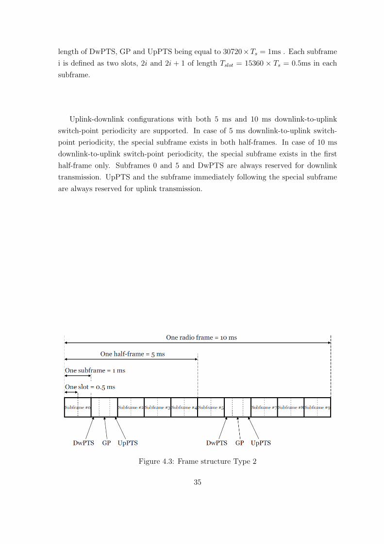
4.4.2 PRACH resources for frame structure type 2:

Frame structure type 2 is applicable to TDD. Each radio frame of length Tf =

307200 × Ts = 10ms consists of two half-frames of length 153600 × Ts = 5ms each.

Each half-frame consists of five subframes of length 30720×Ts = 1ms. The supported

uplink-downlink configurations are listed in Table-?? where, for each subframe in a

radio frame, D denotes the subframe is reserved for downlink transmissions, U denotes

the subframe is reserved for uplink transmissions and S denotes a special subframe

with the three fields DwPTS, GP and UpPTS as shown in Figure ??. The total

34

length of DwPTS, GP and UpPTS being equal to 30720×Ts = 1ms . Each subframe

i is defined as two slots, 2i and 2i + 1 of length Tslot = 15360 × Ts = 0.5ms in each

subframe.

Uplink-downlink configurations with both 5 ms and 10 ms downlink-to-uplink

switch-point periodicity are supported. In case of 5 ms downlink-to-uplink switch-

point periodicity, the special subframe exists in both half-frames. In case of 10 ms

downlink-to-uplink switch-point periodicity, the special subframe exists in the first

half-frame only. Subframes 0 and 5 and DwPTS are always reserved for downlink

transmission. UpPTS and the subframe immediately following the special subframe

are always reserved for uplink transmission.

Figure 4.3: Frame structure Type 2

35

Uplink-

downlink

configuration

Downlink-

to-Uplink

Switch-point

periodicity

Subframe number

0 1 2 3 4 5 6 7 8 9

0 5 ms D S U U U D S U U U

1 5 ms D S U U D D S U U D

2 5 ms D S U D D D S U D D

3 10 ms D S U U U D D D D D

4 10 ms D S U U D D D D D D

5 10 ms D S U D D D D D D D

6 5 ms D S U U U D S U U D

Table 4.3: Uplink-Downlink Configuration Type 2

For frame structure type 2 with preamble format 0 − 4, there might be multi-

ple random access resources in an UL subframe (or UpPTS for preamble format 4)

depending on the UL/DL configuration, as shown in Table-??. Table-?? lists the

mapping to physical resources for the different random access opportunities needed

for corresponding PRACH Configuration-index, which is assigned by higher layers.

Each quadruple of the format (fRA, t0RA, t

1RA, t

2RA) indicates the location of a specific

random access resource, where fRA is a frequency resource index within the consid-

ered time instance, t2RA = 0, 1, 2 indicates whether the resource is reoccurring in all

radio frames, in even radio frames, or in odd radio frames, respectively, t1RA = 0, 1

indicates whether the random access resource is located in first half frame or in sec-

ond half frame, respectively, and where t2RA is the uplink subframe number where

the preamble starts, counting from 0 at the first uplink subframe between 2 consecu-

tive downlink-to-uplink switch points, with the exception of preamble format 4 where

t2RA is denoted as (∗).The start of the random access preamble formats 0 − 3 shall

be aligned with the start of the corresponding uplink subframe at the UE assuming

NTA = 0, and the random access preamble format 4 shall start 4832× Ts before the

end of the UpPTS at the UE, where the UpPTS is referenced to the UEs uplink

frame timing assuming NTA = 0, where NTA = 0 is the timing offset between uplink

and downlink radio frames at the UE, expressed in units of Ts . The random access

opportunities for each PRACH configuration shall be allocated in time first and then

in frequency if and only if time multiplexing is not sufficient to hold all opportunities

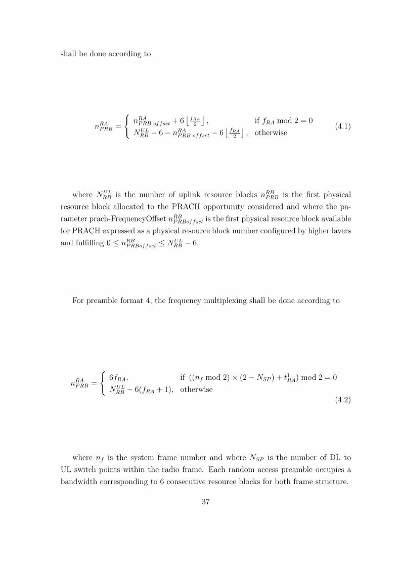
of a PRACH configuration. For preamble format 0 − 3, the frequency multiplexing

36

shall be done according to

nRAPRB =

{nRAPRB offset + 6

⌊fRA

2

⌋, if fRA mod 2 = 0

NULRB − 6− nRAPRB offset − 6

⌊fRA

2

⌋, otherwise

(4.1)

where NULRB is the number of uplink resource blocks nRBPRB is the first physical

resource block allocated to the PRACH opportunity considered and where the pa-

rameter prach-FrequencyOffset nRBPRBoffset is the first physical resource block available

for PRACH expressed as a physical resource block number configured by higher layers

and fulfilling 0 ≤ nRBPRBoffset ≤ NULRB − 6.

For preamble format 4, the frequency multiplexing shall be done according to

nRAPRB =

{6fRA, if ((nf mod 2)× (2−NSP ) + t1RA) mod 2 = 0

NULRB − 6(fRA + 1), otherwise

(4.2)

where nf is the system frame number and where NSP is the number of DL to

UL switch points within the radio frame. Each random access preamble occupies a

bandwidth corresponding to 6 consecutive resource blocks for both frame structure.

37

PRACH UL/DL configuration

configuration Index

0 1 2 3 4 5 6

0 (0,1,0,2) (0,1,0,1) (0,1,0,0) (0,1,0,2) (0,1,0,1) (0,1,0,0) (0,1,0,2)

1 (0,2,0,2) (0,2,0,1) (0,2,0,0) (0,2,0,2) (0,2,0,1) (0,2,0,0) (0,2,0,2)

2 (0,1,1,2) (0,1,1,1) (0,1,1,0) (0,1,0,1) (0,1,0,0) N/A (0,1,1,1)

3 (0,0,0,2) (0,0,0,1) (0,0,0,0) (0,0,0,2) (0,0,0,1) (0,0,0,0) (0,0,0,2)

4 (0,0,1,2) (0,0,1,1) (0,0,1,0) (0,0,0,1) (0,0,0,0) N/A (0,0,1,1)

5 (0,0,0,1) (0,0,0,0) N/A (0,0,0,0) N/A N/A (0,0,0,1)

6 (0,0,0,2) (0,0,0,1) (0,0,0,0) (0,0,0,1) (0,0,0,0) (0,0,0,0) (0,0,0,2)

(0,0,1,2) (0,0,1,1) (0,0,1,0) (0,0,0,2) (0,0,0,1) (1,0,0,0) (0,0,1,1)

7 (0,0,0,1) (0,0,0,0) N/A (0,0,0,0) N/A N/A (0,0,0,1)

(0,0,1,1) (0,0,1,0) (0,0,0,2) (0,0,1,0)

8 (0,0,0,0) N/A N/A (0,0,0,0) N/A N/A (0,0,0,0)

(0,0,1,0) (0,0,0,1) (0,0,1,1)

9 (0,0,0,1) (0,0,0,0) (0,0,0,0) (0,0,0,0) (0,0,0,0) (0,0,0,0) (0,0,0,1)

(0,0,0,2) (0,0,0,1) (0,0,1,0) (0,0,0,1) (0,0,0,1) (1,0,0,0) (0,0,0,2)

(0,0,1,2) (0,0,1,1) (1,0,0,0) (0,0,0,2) (1,0,0,1) (2,0,0,0) (0,0,1,1)

10 (0,0,0,0) (0,0,0,1) (0,0,0,0) N/A (0,0,0,0) N/A (0,0,0,0)

(0,0,1,0) (0,0,1,0) (0,0,1,0) (0,0,0,1) (0,0,0,2)

(0,0,1,1) (0,0,1,1) (1,0,1,0) (1,0,0,0) (0,0,1,0)

11 N/A (0,0,0,0) N/A N/A N/A N/A (0,0,0,1)

(0,0,0,1) (0,0,1,0)

(0,0,1,0) (0,0,1,1)

12 (0,0,0,1) (0,0,0,0) (0,0,0,0) (0,0,0,0) (0,0,0,0) (0,0,0,0) (0,0,0,1)

(0,0,0,2) (0,0,0,1) (0,0,1,0) (0,0,0,1) (0,0,0,1) (1,0,0,0) (0,0,0,2)

(0,0,1,1) (0,0,1,0) (1,0,0,0) (0,0,0,2) (1,0,0,0) (2,0,0,0) (0,0,1,0)

(0,0,1,2) (0,0,1,1) (1,0,1,0) (1,0,0,2) (1,0,0,1) (3,0,0,0) (0,0,1,1)

13 (0,0,0,0) N/A N/A (0,0,0,0) N/A N/A (0,0,0,0)

(0,0,0,2) (0,0,0,1) (0,0,0,1)

(0,0,1,0) (0,0,0,2) (0,0,0,2)

(0,0,1,2) (1,0,0,1) (0,0,1,1)

14 (0,0,0,0) N/A N/A (0,0,0,0) N/A N/A (0,0,0,0)

(0,0,0,1) (0,0,0,1) (0,0,0,2)

(0,0,1,0) (0,0,0,2) (0,0,1,0)

(0,0,1,1) (1,0,0,0) (0,0,1,1)

15 (0,0,0,0) (0,0,0,0) (0,0,0,0) (0,0,0,0) (0,0,0,0) (0,0,0,0) (0,0,0,0)

(0,0,0,1) (0,0,0,1) (0,0,1,0) (0,0,0,1) (0,0,0,1) (1,0,0,0) (0,0,0,1)

(0,0,0,2) (0,0,1,0) (1,0,0,0) (0,0,0,2) (1,0,0,0) (2,0,0,0) (0,0,0,2)

(0,0,1,1) (0,0,1,1) (1,0,1,0) (1,0,0,1) (1,0,0,1) (3,0,0,0) (0,0,1,0)

(0,0,1,2) (1,0,0,1) (2,0,0,0) (1,0,0,2) (2,0,0,1) (4,0,0,0) (0,0,1,1)

16 (0,0,0,1) (0,0,0,0) (0,0,0,0) (0,0,0,0) (0,0,0,0) N/A N/A

(0,0,0,2) (0,0,0,1) (0,0,1,0) (0,0,0,1) (0,0,0,1)

(0,0,1,0) (0,0,1,0) (1,0,0,0) (0,0,0,2) (1,0,0,0)

(0,0,1,1) (0,0,1,1) (1,0,1,0) (1,0,0,0) (1,0,0,1)

(0,0,1,2) (1,0,1,1) (2,0,1,0) (1,0,0,2) (2,0,0,0)

17 (0,0,0,0) (0,0,0,0) N/A (0,0,0,0) N/A N/A N/A

(0,0,0,1) (0,0,0,1) (0,0,0,1)

(0,0,0,2) (0,0,1,0) (0,0,0,2)

(0,0,1,0) (0,0,1,1) (1,0,0,0)

(0,0,1,2) (1,0,0,0) (1,0,0,1)

18 (0,0,0,0) (0,0,0,0) (0,0,0,0) (0,0,0,0) (0,0,0,0) (0,0,0,0) (0,0,0,0)

(0,0,0,1) (0,0,0,1) (0,0,1,0) (0,0,0,1) (0,0,0,1) (1,0,0,0) (0,0,0,1)

(0,0,0,2) (0,0,1,0) (1,0,0,0) (0,0,0,2) (1,0,0,0) (2,0,0,0) (0,0,0,2)

(0,0,1,0) (0,0,1,1) (1,0,1,0) (1,0,0,0) (1,0,0,1) (3,0,0,0) (0,0,1,0)

(0,0,1,1) (1,0,0,1) (2,0,0,0) (1,0,0,1) (2,0,0,0) (4,0,0,0) (0,0,1,1)

(0,0,1,2) (1,0,1,1) (2,0,1,0) (1,0,0,2) (2,0,0,1) (5,0,0,0) (1,0,0,2)

19 N/A (0,0,0,0) N/A N/A N/A N/A (0,0,0,0)

(0,0,0,1) (0,0,0,1)

(0,0,1,0) (0,0,0,2)

(0,0,1,1) (0,0,1,0)

(1,0,0,0) (0,0,1,1)

(1,0,1,0) (1,0,1,1)

20 / 30 (0,1,0,1) (0,1,0,0) N/A (0,1,0,1) (0,1,0,0) N/A (0,1,0,1)

21 / 31 (0,2,0,1) (0,2,0,0) N/A (0,2,0,1) (0,2,0,0) N/A (0,2,0,1)

22 / 32 (0,1,1,1) (0,1,1,0) N/A N/A N/A N/A (0,1,1,0)

23 / 33 (0,0,0,1) (0,0,0,0) N/A (0,0,0,1) (0,0,0,0) N/A (0,0,0,1)

24 / 34 (0,0,1,1) (0,0,1,0) N/A N/A N/A N/A (0,0,1,0)

38

PRACH UL/DL configuration

configuration Index

0 1 2 3 4 5 6

25 / 35 (0,0,0,1) (0,0,0,0) N/A (0,0,0,1) (0,0,0,0) N/A (0,0,0,1)

(0,0,1,1) (0,0,1,0) (1,0,0,1) (1,0,0,0) (0,0,1,0)

26 / 36 (0,0,0,1) (0,0,0,0) (0,0,0,1) (0,0,0,0) (0,0,0,1)

(0,0,1,1) (0,0,1,0) N/A (1,0,0,1) (1,0,0,0) N/A (0,0,1,0)

(1,0,0,1) (1,0,0,0) (2,0,0,1) (2,0,0,0) (1,0,0,1)

27 / 37 (0,0,0,1) (0,0,0,0) (0,0,0,1) (0,0,0,0) (0,0,0,1)

(0,0,1,1) (0,0,1,0) N/A (1,0,0,1) (1,0,0,0) N/A (0,0,1,0)

(1,0,0,1) (1,0,0,0) (2,0,0,1) (2,0,0,0) (1,0,0,1)

(1,0,1,1) (1,0,1,0) (3,0,0,1) (3,0,0,0) (1,0,1,0)

28 / 38 (0,0,0,1) (0,0,0,0) (0,0,0,1) (0,0,0,0) (0,0,0,1)

(0,0,1,1) (0,0,1,0) (1,0,0,1) (1,0,0,0) (0,0,1,0)

(1,0,0,1) (1,0,0,0) N/A (2,0,0,1) (2,0,0,0) N/A (1,0,0,1)

(1,0,1,1) (1,0,1,0) (3,0,0,1) (3,0,0,0) (1,0,1,0)

(2,0,0,1) (2,0,0,0) (4,0,0,1) (4,0,0,0) (2,0,0,1)

29 /39 (0,0,0,1) (0,0,0,0) (0,0,0,1) (0,0,0,0) (0,0,0,1)

(0,0,1,1) (0,0,1,0) (1,0,0,1) (1,0,0,0) (0,0,1,0)

(1,0,0,1) (1,0,0,0) N/A (2,0,0,1) (2,0,0,0) N/A (1,0,0,1)

(1,0,1,1) (1,0,1,0) (3,0,0,1) (3,0,0,0) (1,0,1,0)

(2,0,0,1) (2,0,0,0) (4,0,0,1) (4,0,0,0) (2,0,0,1)

(2,0,1,1) (2,0,1,0) (5,0,0,1) (5,0,0,0) (2,0,1,0)

40 (0,1,0,0) N/A N/A (0,1,0,0) N/A N/A (0,1,0,0)

41 (0,2,0,0) N/A N/A (0,2,0,0) N/A N/A (0,2,0,0)

42 (0,1,1,0) N/A N/A N/A N/A N/A N/A

43 (0,0,0,0) N/A N/A (0,0,0,0) N/A N/A (0,0,0,0)

44 (0,0,1,0) N/A N/A N/A N/A N/A N/A

45 (0,0,0,0) N/A N/A (0,0,0,0) N/A N/A (0,0,0,0)

(0,0,1,0) (1,0,0,0) (1,0,0,0)

46 (0,0,0,0) (0,0,0,0) (0,0,0,0)

(0,0,1,0) N/A N/A (1,0,0,0) N/A N/A (1,0,0,0)

(1,0,0,0) (2,0,0,0) (2,0,0,0)

47 (0,0,0,0) (0,0,0,0) (0,0,0,0)

(0,0,1,0) N/A N/A (1,0,0,0) N/A N/A (1,0,0,0)

(1,0,0,0) (2,0,0,0) (2,0,0,0)

(1,0,1,0) (3,0,0,0) (3,0,0,0)

48 (0,1,0,*) (0,1,0,*) (0,1,0,*) (0,1,0,*) (0,1,0,*) (0,1,0,*) (0,1,0,*)

49 (0,2,0,*) (0,2,0,*) (0,2,0,*) (0,2,0,*) (0,2,0,*) (0,2,0,*) (0,2,0,*)

50 (0,1,1,*) (0,1,1,*) (0,1,1,*) N/A N/A N/A (0,1,1,*)

51 (0,0,0,*) (0,0,0,*) (0,0,0,*) (0,0,0,*) (0,0,0,*) (0,0,0,*) (0,0,0,*)

52 (0,0,1,*) (0,0,1,*) (0,0,1,*) N/A N/A N/A (0,0,1,*)

53 (0,0,0,*) (0,0,0,*) (0,0,0,*) (0,0,0,*) (0,0,0,*) (0,0,0,*) (0,0,0,*)

(0,0,1,*) (0,0,1,*) (0,0,1,*) (1,0,0,*) (1,0,0,*) (1,0,0,*) (0,0,1,*)

54 (0,0,0,*) (0,0,0,*) (0,0,0,*) (0,0,0,*) (0,0,0,*) (0,0,0,*) (0,0,0,*)

(0,0,1,*) (0,0,1,*) (0,0,1,*) (1,0,0,*) (1,0,0,*) (1,0,0,*) (0,0,1,*)

(1,0,0,*) (1,0,0,*) (1,0,0,*) (2,0,0,*) (2,0,0,*) (2,0,0,*) (1,0,0,*)

55 (0,0,0,*) (0,0,0,*) (0,0,0,*) (0,0,0,*) (0,0,0,*) (0,0,0,*) (0,0,0,*)

(0,0,1,*) (0,0,1,*) (0,0,1,*) (1,0,0,*) (1,0,0,*) (1,0,0,*) (0,0,1,*)

(1,0,0,*) (1,0,0,*) (1,0,0,*) (2,0,0,*) (2,0,0,*) (2,0,0,*) (1,0,0,*)

(1,0,1,*) (1,0,1,*) (1,0,1,*) (3,0,0,*) (3,0,0,*) (3,0,0,*) (1,0,1,*)

56 (0,0,0,*) (0,0,0,*) (0,0,0,*) (0,0,0,*) (0,0,0,*) (0,0,0,*) (0,0,0,*)

(0,0,1,*) (0,0,1,*) (0,0,1,*) (1,0,0,*) (1,0,0,*) (1,0,0,*) (0,0,1,*)

(1,0,0,*) (1,0,0,*) (1,0,0,*) (2,0,0,*) (2,0,0,*) (2,0,0,*) (1,0,0,*)

(1,0,1,*) (1,0,1,*) (1,0,1,*) (3,0,0,*) (3,0,0,*) (3,0,0,*) (1,0,1,*)

(2,0,0,*) (2,0,0,*) (2,0,0,*) (4,0,0,*) (4,0,0,*) (4,0,0,*) (2,0,0,*)

57 (0,0,0,*) (0,0,0,*) (0,0,0,*) (0,0,0,*) (0,0,0,*) (0,0,0,*) (0,0,0,*)

(0,0,1,*) (0,0,1,*) (0,0,1,*) (1,0,0,*) (1,0,0,*) (1,0,0,*) (0,0,1,*)

(1,0,0,*) (1,0,0,*) (1,0,0,*) (2,0,0,*) (2,0,0,*) (2,0,0,*) (1,0,0,*)

(1,0,1,*) (1,0,1,*) (1,0,1,*) (3,0,0,*) (3,0,0,*) (3,0,0,*) (1,0,1,*)

(2,0,0,*) (2,0,0,*) (2,0,0,*) (4,0,0,*) (4,0,0,*) (4,0,0,*) (2,0,0,*)

(2,0,1,*) (2,0,1,*) (2,0,1,*) (5,0,0,*) (5,0,0,*) (5,0,0,*) (2,0,1,*)

58 N/A N/A N/A N/A N/A N/A N/A

59 N/A N/A N/A N/A N/A N/A N/A

60 N/A N/A N/A N/A N/A N/A N/A

61 N/A N/A N/A N/A N/A N/A N/A

62 N/A N/A N/A N/A N/A N/A N/A

63 N/A N/A N/A N/A N/A N/A N/A

Table 4.4: Frame structure type2

39

4.5 Preamble sequence design

In Random access process multiple users may be transmitting randomly chosen pream-

bles on same time-frequency resources, and hence all these preambles from multiple

users must be orthogonal to each other or else it may lead to serious interference

among these transmitted preambles leading to failure of random access process.The

sequence that is to be transmitted as a preamble should be appropriately chosen such

that it should be able to provide orthogonality among different transmitted preambles

and also the selected sequence should minimize the overhead on PRACH transmission

and it should meet the power requirements.

Considering the above constraints laid on the preamble sequence, a special se-

quence termed as prime-length ZadoffChu (ZC) sequences have been chosen to gener-

ate the preamble sequence. ZC sequences are non-binary unit-amplitude sequences,

which satisfy a Constant Amplitude Zero Autocorrelation (CAZAC) property. The

ZC sequence of odd-length NZC is given by

xu(n) = e−j2πun(n+1)+ln

NZC (4.3)

Where u={ 0,1,...,NZC } is the ZC sequence root index

n={0,1,2,...,NZC}l=any integer.But in LTE we take l=0 for simplicity.

Pseudo-Noise (PN) based sequences were used in WCDMA(wide band CDMA)

for random access process, in LTE prime-length ZadoffChu (ZC) sequences are used.

Zadoff-chu sequence comes with many attractive properties; three among them which

are very much important in dealing with synchronization and minimizing interference

is given below

• A ZC sequence has a constant amplitude and also its NZC point DFT also has a

constant amplitude. This property limits the Peak-to-Average Ratio and generates

bounded and time-flat interference to other users

• ZC sequences of any length have ideal cyclic autocorrelation (i.e. the correlation

with its circularly shifted version is a delta function). The zero autocorrelation prop-

erty may be formulated as:

rkk =

NZC−1∑n=0

xu(n)x∗u(n+ σ) = δ(σ) (4.4)

where rkk(.) is the discrete periodic autocorrelation function of xu at lag σ. This

40

property is of major interest when the received signal is correlated with a reference

sequence and the received reference sequences are misaligned.

• The absolute value of the cyclic cross-correlation function between any two ZC

sequences is constant and equal to 1/√NZC if |u1− u2| (where u1 and u2 are the

sequence root indices) ) is relatively prime with respect to (a condition that can be

easily guaranteed if NZC is a prime number).

4.5.1 Zadoff-Chu(ZC)sequence length

The sequence length design should address the following requirements:

• Maximize the number of ZC sequences with optimal cross-correlation properties.

• Minimize the interference to/from the surrounding scheduled data on the PUSCH.

The former requirement is guaranteed by choosing a prime-length Zadoff-chu(ZC)

sequence.For the latter, since data and preamble OFDM symbols are neither aligned

nor have the same durations, strict orthogonality cannot be achieved. At least, fixing

the preamble duration to an integer multiple of the PUSCH symbol provides some

compatibility between preamble and PUSCH subcarriers. However, with the 800µs

duration, the corresponding sequence length would be 864, which does not meet the

prime number requirement for length of ZC sequence. The PRACH uses guard bands

to avoid the data interference at preamble edges..In the absence of interference, there

is no significant performance difference between sequences of similar prime length. In

the presence of interference, it can be seen that reducing the ZC-sequence length below

839 gives no further improvement in detection rate. No effect is observed on the false

alarm rate. Therefore the ZC-sequence length of 839 is selected for LTE PRACH,

corresponding to 69.91 PUSCH subcarriers in each SC-FDMA symbol, and offers

72− 69.91 = 2.09 PUSCH subcarriers protection, which is very close to one PUSCH

subcarrier protection on each side of the preamble. So the preamble is positioned

centrally in the block of 864 available PRACH subcarriers, with 12.5 null subcarriers

on each side.

4.5.2 Random Access cyclic shifts

Each cell needs to generate 64 different preambles from ZC-sequence of length 839

samples and all of these preambles should be be orthogonal to each other so as to avoid

any sort of interference among different RACH transmissions on same time-frequency

resource,in such case by exploiting the cyclic auto correlation of ZC sequence if all

41

preambles can be generated from same root sequence then all of them will be or-

thonormal to each other, but it is not possible in all cases. For small cells which

typically are less than 1km this may be possible but however for large cells generat-

ing all 64 signatures (all orthogonal to each other) from a single root sequence is not

possible.The cyclic shift offset NCS configured by eNodeB dictates the preamble gen-

eration from root sequence, it specifies with how many samples a given root sequence

should cyclically shifted to ensure orthogonality among different preambles.The cyclic

shift offset NCS is dimensioned so that the Zero Correlation Zone (ZCZ) of the se-

quences guarantees the orthogonality of the PRACH sequences regardless of the delay

spread and time uncertainty of the UEs. The minimum value of NCS should therefore

be the smallest integer number of sequence sample periods that is greater than the

maximum delay spread and time uncertainty of an uplink non-synchronized UE,plus

some additional guard samples provisioned for the spill-over of the pulse shaping fil-

ter envelope present in the PRACH receiver.As delay spread and timing uncertainty

of large cells are high and hence NCS value will also be high and with that high

cyclic shift value it is not possible to generate all 64 preambles with a single root

sequence and hence for large cells multiple root sequences are employed to generate

all required preamble signatures.Some cell scenarios and their corresponding cyclic

shift values and their coverage range are shown in Table: ??

Cell scenario No of Cyclic shifts No of ZC root Cyclic Shift Cell Radius

Per ZC sequence Sequences Size NCS In Km

1 64 1 13 0.7

2 32 2 26 2.5

3 18 4 46 2.5

4 9 8 93 12

Table 4.5: Different cell scenarios and their corresponding cyclic shifts and their

typical coverage

Cyclic shift offset NCS is specified by eNodeB and falls in range of 13 to 839 and

hence to configure it by eNodeB,it requires to transmit 10 bit value corresponding to a

particular cyclic shift as a part of system information ,instead to avoid transmission of

10 bit string , all possible cyclic shift values corresponding to all formats are quantized

to just 16 values .The 16 allowed values of NCS were chosen so that the number of

orthogonal preambles is as close as possible to what could be obtained if there were

no restrictions on the value of NCS. The 16 quantized set of cyclic shift offset values

42

and corresponding formats to be used are given in Table:??.

Cyclic prefix Format Range in Km

Offset NCS

13 0 0.79

15 0 1.08

18 0 1.51

22 0 2.08

26 0 2.65

32 0 3.51

38 0 4.37

46 0 5.51

59 0 7.37

76 0 9.8

93 2 12.23

119 2 15.95

167 1,3 22.82

279 1,3 38.84

419 1,3 58.86

839 1,3 118

Table 4.6: Quantized cyclic shift offset values for low speed cells

For a given cell, based on its radius a cyclic shift offset value, NCS is configured

by eNodeB and is transmitted via broadcast channel as a part of system information,

and different cyclic shift values (Cv) are derived from configured cyclic shift offset

using the relation

Cv =

{v.NCS where v = 1, 2, 3, ..., NZC/NCS

0 for NCS = 0(4.5)

Once we get Cv, we can generate multiple preambles by circular shifting of the

given ZC-sequence of root index u using the following function

xu,v(n) = xu((n+ Cv) modNZC) (4.6)

43

4.5.3 Baseband prach signal generation

The time-continuous random access signal s(t) is defined by

s (t) = βPRACH

NZC−1∑k=0

NZC−1∑n=0

xu,v(n) · e−j2πnkNZC · ej2π(k+φ+K(k0+1�2 ))∆fRA(t−TCP) (4.7)

where 0 ≤ t < Tseq + TCP

βPRACH is an amplitude scaling factor in order to conform to the transmit power

k0 = nRBPRBNRBSC −NUL

RBNRBSC /2

NULRB :The uplink system bandwidth (in RBs).

NRBSC :The number of subcarriers per RB, i.e. 12.

nRAPRB:It is the parameter which controls the location in the frequency domain, ex-

pressed as a resource block number configured by higher layers and fulfilling

0 ≤ nRBPRB < NULRB − 6

K = ∆f/∆fRA accounts for the ratio of subcarrier spacing between the PUSCH and

PRACH

φ: a fixed offset determining the frequency-domain location of the random access

preamble within the physical resource blocks.The variable ∆fRA and φ values for

different preamble formats are given in the Table:??

Preamble format ∆fRA φ

0 - 3 1250 Hz 7

4 7500 Hz 2

Table 4.7: Random access baseband parameters

44

Chapter 5

PRACH Implementation

5.1 UE Tramsmitter

At UE PRACH can be generated on the assigned time frequency resource in one of

the two ways:

• Full frequency domain

• Hybrid time/frequency domain

5.1.1 Full frequency domain

In this method PRACH preamble is generated just like as a normal OFDM symbol

at the system sampling rate, where the samples are DFT precoded (optional) and

an IDFT block preceded with subcarrier mapping is used for preamble generation, in

order to support large cells the same preamble sequence is repeated to lengthen the

sequence as discussed in preamble formats and a cyclic prefix is appended to ensure

frequency domain processing at receiver and the same is shown in Figure:??

45

Figure 5.1: Full frequency domain PRACH transmitter

The method described above does not require any time-domain filtering at base-

band, but leads to large IDFT sizes (up to 24576 for a 20 MHz spectrum allocation),

which are cumbersome to implement in practice.

5.1.2 Hybrid time/frequency domain

The concept behind this method is to use a smaller size IFFT instead of using a

very large size IDFT, and shifting the preamble to the required frequency location

through time-domain upsampling and filtering, as shown in figure ?? . Given that

the preamble sequence length is 839, the smallest IFFT size that can be used is

1024, resulting in a sampling frequency of fIFFT = 1.28 Msps. Both the CP and the

sequence durations have been designed to provide an integer number of samples at

this sampling rate. The CP can be inserted before the upsampling and time-domain

frequency shift, so as to minimize the intermediate storage requirements.

Figure 5.2: Hybrid frequency/time domain PRACH generation

46

5.2 PRACH Receiver

The receiver at the eNodeB can also be chosen between Full frequency domain and

Hybrid time/Frequency domain,as shown in Figure ??.In full frequency domain the

computation of frequency tones carrying the PRACH signals is carried out directly

from the received 800µs duration signal with in observation interval, the full range of

frequency tones used for uplink transmission given the system bandwidth.It does not

require any time domain filtering or frequency shifts but demands for a large sized

DFT.

The hybrid time/frequency-domain method first extracts the relevant PRACH

signal through a time-domain frequency shift with down-sampling and anti-aliasing

filtering. There follows a small-size DFT computing the set of frequency tones cen-

tered on the PRACH tones, which can then be extracted.The down-sampling ratio

and corresponding anti-aliasing filter are chosen to deliver a number of PRACH time

samples suitable for an FFT or simple DFT computation at a sampling rate which is

an integer fraction of the system sampling rate.

Figure 5.3: PRACH receiver

5.2.1 Power delay profile computation

Power delay profile of a PRACH preamble is computed as a discrete periodic correla-

tion between received sequence y(n) and the reference searched NZC length Zadoff-chu

47

sequence xu(n).Cyclic prefix appended at transmitter ensures the frequency domain

periodic correlation at receiver, and minimizes the computational complexity for PDP

computation.The following section describes how to compute the PDP profile of each

preamble.The discrete periodic correlation, zu(l) at lag l between the received se-

quence y(n) and reference sequence xu(n) is given as

|zu (l)|2 =

∣∣∣∣∣NZC−1∑n=0

y(n)x∗u [(n+ l)NZC ]

∣∣∣∣∣2

(5.1)

zu(l) can also be expressed as follows

zu(l) = [y(n) ∗ x∗u(−n)] (l) (5.2)

Let Xu(k) = RXu(k) + jIXu(k), Yu(k) = RY (k) + jIY (k) and Zu(k) be the DFT

coefficients of the time-domain ZC sequence xu(n) , the received baseband samples

y(n), and the discrete periodic correlation function zu(n) respectively. Using the

properties of the DFT, Zu(n) can be efficiently computed in the frequency domain as

Zu(k) = Y (K)X∗u(k) for k = 0, ..., NZC − 1 (5.3)

zu(n) can be computed by taking IDFT of Zu(k) which is given as

zu(n) =

NZC−1∑k=0

Zu(k)ej2πkn/NZC for n = 0, ..., NZC − 1 (5.4)

The received signal in frequency domain is complex-conjugate multiplied with fre-

quency domain root ZC sequence. Due to the fact that frequency domain complex

multiplication with root ZC sequence is equal to time domain cyclic correlation, IFFT

of the multiplied sequence gives time domain cyclic correlation .

5.2.2 Sequence detection

The PRACH signatures which are transmitted are generated from cyclic shifts of a

common root sequence means that frequency-domain computation of a root sequence

provides in one shot the concatenated PDP’s of all signatures derived from the same

root sequence.Therefore, the signature detection process consists of searching, within

each ZCZ(Zero Correlation Zone) defined by each cyclic shift, the PDP peaks above

a detection threshold over a search window corresponding to the cell size.Figure:??

48

shows the basic function of signature detection

Figure 5.4: Signature detection per root sequence

The noise-floor threshold function collects the PDP output and estimates the

absence or presence of an RA preamble by predefined threshold level. If the noise-

floor threshold function detects the existence of RA preamble in received signal, peak

searching function estimates preamble ID and propagation delay. Due to the unique

correlation properties of ZC sequence as described previously, the preamble ID can

be indicated by the peak position information and its cyclic shift value Cv. If the

RA preamble is received with certain amount of propagation delay, the peak position

information is effected by not only Cv but also the amount of delay.As described in

Figure:??, the position of the peak is delayed in temporal domain by the quantity of

propagation delay. According to this, the preamble detection module can estimate

Preamble ID and its propagation delay exactly if the quantity of propagation delay

in time domain is less than unit cyclic shift value.

Figure 5.5: PRACH preamble detection

49

5.2.3 Noise floor estimation and threshold calculation

Noise floor can be calculated by considering transmission of only Gaussian noise, in

the absence of preamble. The noise floor can be estimated as follows

γ(n) =1

Ns

Ns−1∑i=0

znca(i) (5.5)

where Ns is the number of samples in the search window, and znca(i) is given by the

following expression

znca(i) =Na∑a=1

Nnca−1∑m=0

|zma (i)|2 (5.6)

where Na is the number of antennas, Nnca is the number of additional non-coherent

accumulations(e.g in case of sequence repetition preamble format) and |zma (i)|2 is the

PDP output for a particular antenna. znca(i) follows a central chi-square distribution

with 2N = 2Na.Nnca degrees of freedom with Cumulative Density Function F (Tdet) =

1−pfa(Tdet)Ns where Ns is number of samples in search window and Tdet is the desired

absolute threshold.The target false alarm probability pfa(Tdet) drives the setting of

the detection threshold Tdet(The initial absolute threshold value is computed using

an initial noise floor estimated by averaging across all search window samples).It is

worth noticing that instead of the absolute threshold we can consider the threshold

Tr relative to the noise floor γ(n) as follows:

Tr = Tdet/γ(n) (5.7)

This removes the dependency of F (Tr) on the noise variance:

F (Tr) = 1− e−Na.NncaTrNa.Nnca−1∑

k=0

1

k!(Na.NncaTr)

k (5.8)

As a result, the relative detection threshold can be precomputed and stored. F (Tr)

refers to the probability of PDP output samples(which in this case is obtained by just

transmitting noise) less than relative threshold Tr and 1− F (Tr) gives probability of

false alarm.The target false alarm probability drives the setting of absolute threshold

Tdet.

50

Chapter 6

Results

Link level simulations have been carried out for evaluating the performance of the

algorithms.The proposed algorithms have also been applied to real time RF cap-

tured data from MW1000 test bed to verify the applicability of the algorithms in

real time.The 20 MHz LTE system was considered, with a sampling frequency of

fs = 30.72MHz, N = 2048-point FFT/IFFT,144-sample CP and a 15kHz subcarrier

spacing.The maximum channel delay spread was 1.07µs, corresponding to 32 channel

taps by considering system sampling frequency fs.A frequency offset of 127kHz, which

corresponds to ε = 8.47 has been considered.Only one antenna at the transmitter and

receiver has been considered.

Figure ?? shows the simulation results of time domain correlation for PSS detec-

tion for one complete radio frame at SNR=0dB with two interferences considered with

powers −2dB and −3dB . In this figure magnitude of correlation is plotted against

sample location corresponding to single radio frame. Further it can be observed from

Figure ?? that location of both the PSS in the given radio frame can be roughly

estimated from the two dominant peaks. Whereas Figure ?? shows the time do-

main correlation for PSS detection for a real time RF captured signal from MW 1000

test bed.The received signal strength is 25mW which corresponds to −16dB.Sample

location represents the time domain sample index while considering only one radio

frame.

51

Figure 6.1: Simulation result of time domain correlation for PSS detection with in-

terference

Figure 6.2: Time domain correlation for PSS detection for real time captured signal

Figure ?? illustrates the time coarse estimation based on Cyclic Prefix(CP) cor-

relation.The magnitude of the CP correlation is plotted against the relative position

from the estimation of the PSS location obtained from the time domain correlation

for PSS detection as shown in Figure ??. Similarly Figure ?? represents the CP

correlation for a real time RF captured signal from MW 1000 test bed.The loca-

tion corresponds to the CP correlation peak value as shown in the Figure ?? and

Figure ?? gives the position where CP of the OFDM signal corresponding to PSS

actually starts.Once the starting location of CP is obtained PSS and hence SSS can

be obtained based on there known relative positions in terms of number of OFDM

symbols.

52

Figure 6.3: CP based correlation for simulated data

Figure 6.4: CP based correlation for real time RF captured data

2D-MMSE channel estimation is also performed on both PSS and SSS after detect-

ing the correct cell-ID, to compare the results to that of an ideal case.Figure ?? repre-

sents the ideal constellation plot for PSS ZC-sequence in frequency domain.Figure ??

illustrates the PSS ZC-sequence constellation plot in frequency domain obtained after

channel estimation for the real time captured data from MW 1000 test bed.Figure ??

represents the ideal constellation plot for SSS in frequency domain which is nothing

but BPSK modulation.Figure ?? gives the constellation plot for the SSS in frequency

domain after performing channel estimation on real time RF captured signal.

53

Figure 6.5: Ideal Constellation plot for PSS ZC-sequence in frequency domain

Figure 6.6: Received constellation plot for PSS ZC-sequence for real time RF captured

data

54

Figure 6.7: Ideal constellation plot for SSS signal in frequency domain

Figure 6.8: Received constellation plot for SSS signal for real time RF captured signal

Figure ?? illustrates the detection of multiple UE’s transmitting different PRACH

preamble over real time wireless channel.In this figure Power delay profile(PDP) is

plotted against the samples in time domain related to the length of ZC sequence

which is equal to 839 in case of PRACH transmission.There are 9 different UE’s

transmitting 9 different preambles which have been transmitted and captured over real

time channel.Figure ?? shows detection of all the 9 different preambles, corresponding

to 9 different peaks .The preamble number can be obtained based on the location of

the preamble peaks.

55

Figure 6.9: Multiple UE’s detection for PRACH transmission over real time channel

56

Chapter 7

Conclusions and Future Work

For a 3GPP LTE receiver,a cross-correlation approach is proposed to estimate the

sector-ID from PSS in time domain instead of shifting time window each time by

one sample converting it into frequency domain and performing cross-correlation of

Zadoff-chu sequence in frequency domain whereas frequency domain correlation needs

to be performed on SSS to estimate group ID and hence enable cell identification. It

also provides a reliable estimate of the beginning of frame and estimates fractional

frequency offsets based on cyclic prefix correlation. However, for timing acquisition

the low-complexity cyclic prefix based autocorrelation should be preferred, as it is

not influenced by frequency errors.In this work, estimation of large frequency off-

set and cell search are jointly performed with the secondary synchronization signal.

Uplink synchronization has been obtained based on either by hybrid time frequency

domain approach or full frequency domain approach followed for PRACH preamble

detection and estimating the propagation delays of multiple UE’s .The complete pro-

cedure enables a robust connection to the base station at a reasonable implementation

complexity.

Future work includes correction of the FFT window drift caused by the sampling

clock offset.Sampling clock offset errors include the clock phase errors and the clock

frequency error.The clock phase error are similar to the symbol timing error and the

clock phase error can be treated as a kind of the symbol timing error. The sampling

clock frequency errors can cause the ICI.The sampling clock frequency errors can

be detected along with carrier frequency offset from the scheme mentioned in this

thesis.The clock phase error, which leads to FFT window drift needs to be tracked

and has to be compensated inorder to obtain perfect timing synchronization.

57

References

[1] 3GPP TS36-211(v9.1.0), “Physical channels and modulation”, Mar. 2010

[2] J.J van de Beek, M. Sandell and P. O Borjesson, “ML Estimation of Time and

Frequency Offset in OFDM Systems”, IEEE Trans. Signal processing, vol. 45, no.

7, July 1997.

[3] L. J. Cimini,“Analysis and simulation of a digital mobile channel using orthogonal

frequency division multiplexing”, IEEE Trans. Commun., vol. 33, pp. 665-675,

July 1985.

[4] K. Manolakis, et al., “A closed concept for synchronization and cell search in

3GPP LTE systems”, in Proc. IEEE Wireless Communications and Networking

Conference, April 2009.

[5] P.-Y. Tsai and H.-W. Chang, “A new cell search scheme in 3GPP long term evolu-

tion downlink OFDMA systems”, in Proc. International Conference on Wireless

Communications and Signal Processing, Nov. 2009.

[6] H.-G. Park, I.-K. Kim and Y. -S. Kim, “Efficient coherent neighbour cell search

for synchronous 3GPP LTE system”, IET Electron. Lett., 2008, 44, (21), pp.

1267-1268.

[7] J. J. van de Beek, M. Sandell, M. Isaksson, and P. O. Borjesson,“ Lowcomplex

frame synchronization in OFDM systems”, in Proc. IEEE Int. Conf. Universal

Personal Commun., Nov. 1995, pp. 982-986.

[8] K. Manolakis and V. Jungnickel, “Synchronization and Cell Search for 3GPP

LTE”, 13th International OFDM Workshop (InOWo08), August 2008.

[9] M.Sandell, J.J. v.d. Beek and P.O.Borjesson, Timing and Frequency Synchroniza-

tion in OFDM Systems Using the Cyclic Prefix, Proc. IEEE Int. Symp. Synchro-

nization, Essen, Germany, Dec. 1995.

58

[10] Yinigmin Tsai and Guodong Zhang, “Time and Frequency Synchronization for

3GPP LTE Long Term Evolution Systems, IEEE Vehicular Technology Confer-

ence, 65th VTC2007-Spring, April 2007.

[11] M. Speth, F. Classen, and H. Meyr, “Frame synchronization of OFDM systems

in frequency selective fading channels”, in Proc. VTC97, pp. 1807-1811.

[12] J. G. Proakis, Digital Communications, McGraw-Hill, 4th edition, 2001.

[13] . F. Khan, LTE for 4G Mobile Broadband: Air Interface Technologies and Per-

formance, Cambridge University Press, 2009.

[14] M. Speth, S.A. Fechtel, G. Fock and H. Meyr, “Optimum Receiver Design for

Wireless Broad-Band Systems Using OFDM - Part I, IEEE Transactions on Com-

munications, Vol.47, No. 11, November 1999.

[15] M. Speth, S.A. Fechtel, G. Fock and H. Meyr, “Optimum Receiver Design for

Wireless Broad-Band Systems Using OFDM - Part II, IEEE Transactions on

Communications, Vol.49, No. 4, April 2001.

[16] S. B. Weinstein and P. M. Ebert, “Data Transmission by Frequency-Division

Multiplexing using the Discrete Fourier Transform”, IEEE Trans. on Communi-

cations, Vol. 19, pp. 628634, October 1971.

[17] S. Sesia, I. Toufik, and M. Baker, LTE- The UMTS Long Term Evolution From

theory to Practice, John Wiley and Sons Ltd., 2009.

[18] W. C. Jakes, Microwave Mobile Communications, Wiley, 1974.

[19] P. H. Moose, “A technique for orthogonal frequency division multiplexing fre-

quency offset correction, IEEE Trans. Commun., vol. 42, pp. 29082914, Oct. 1994.

[20] B. Yang, Khaled B. Lataef, Roger S. Cheng, Z. Chao, “Timing Recovery for

OFDM Transmission, IEEE Journal on Communications, Vol. 18, No. 11, Novem-

ber 2000.

[21] Erik Dahlman, Stefan Parkvall and Per Beming, “3G Evolution HSPA and LTE

for Mobile Broadband, Academic Press, 2008.

59