Satellite positioning systems are used within the aviationsector extensively. A three-dimensional global navigation satel-lite system (GNSS) enables an aircraft to determine its position(latitude, longitude, and altitude) anywhere on or above theearth. Data transmitted from a navigation and communicationsatellite provides the user with the time, the precise orbitalposition of the satellite and the position of other satellites inthe system. In the past, they were only applied for militarypurposes. However nowadays they are used for a wide rangeof civil aviation applications, including navigation, communi-cation, tracking, and flight management.
A number of previous EC projects such as GADEROS,GRAIL, LOCASYS, and SATLOC, have proved the feasibil-ity of introducing GNSS in non-critical systems by meansof theoretical studies and demonstrations. The current ECproject “European Train Control System Advanced Testingand Smart Train Positioning System” (EATS) [1] proposes anovel positioning system based on different techniques thathave proved useful from other industry viewpoints such asusing information sources from GNSS, UMTS, and GSM.Furthermore, reliability, availability, maintainability, and safety(RAMS) [2]–[4] is proposed as a measure to analyse thedependability of both mission-critical and safety-critical ap-plications.
Availability requirements are identified as the most chal-lenging obstacles towards GNSS aided positioning systems in[2]. Many approaches can be used to analyse the availabilityproperties. Among them, simulation, analytical analysis, and
numerical analysis are popular and practical. Each of them hasits advantages and disadvantages that we do not discuss in thispaper. We consider probabilistic model checking, a numericalanalysis technique based on Markov models. It is a formalmethod for analysing and verifying quantitative properties ofsystems such as as time, stochastic behaviour or resources.It is therefore highly suitable for modelling characteristicsof our system. The basic idea is to first build a (discrete-time or continuous-time) Markov chain or Markov decisionprocess that captures the behaviour of the system, and then touse the model to analyse precisely specified properties usingsome temporal logics. This analysis is automatically performedby using the PRISM model checker [5], and it involves acombination of a traversal of the state transition system ofthe model and numerical computation.
A PRISM specification can be generated directly via aMarkov chain variant described using the PRISM reactivemodules language [6]. Alternatively, a high level model (usingtimed automata, or a process algebra, say) can be translatedinto the PRISM language. According to PRISM’s manual, thelatter approach can be more efficient than the former. This isdue to the fact that PRISM is a symbolic model checker andthe underlying data structures used to represent the systemspecification may function better when there is a high-levelstructure and regularity to exploit.
In this paper we first specify the communication betweenan aircraft and the associated satellites, taking into accounttheir combined mobility. We then analyse the models of theaircraft and satellite set independently before the combinedsystem. Note that behaviour of the system contain a high levelof uncertainty (e.g., in signal transmission unreliability due tosolar radiation). In all our models we specify the system usingthe probabilistic ⇡-calculus. Since PRISM only model checksexpressions in the reactive modules language, and this does notallow for component mobility, so it is not currently possible tomodel check the underlying process algebraic models directly.In order to allow for automatic verification using PRISM, theunderlying continuous-time Markov chains (CTMCs) semanticmodels of our specification are first constructed using rulespresented in [7].
Our paper is organised as follows. In Section II we describethe underlying GNSS based positioning systems. In SectionIII the use of probabilistic model checking is introduced. In
Section IV we present our formal model of the system for anavigation mission of a specific aircraft in the probabilistic ⇡-calculus and its associated CTMC model respectively. Then,we analyse availability properties using the PRISM modelchecker in Section V. The related work is given in SectionVI. Finally, in Section VII we conclude the paper and proposefuture work.
II. GNSS BASED POSITIONING SYSTEMS
A GNSS consists of three major parts: space segment,control segment and user segment. Failure of any subsystemwill lead to errors in the final positioning. Fig. 1 illustratestypical GNSS segments. First, the monitor stations (MS)measure the pseudo-range of visible satellites and send the datato the master control station (MCS). The MCS is responsiblefor collecting and tracking data from each monitor station andcalculating the satellite orbit and clock parameters using aKalman filter. The results are transmitted to ground antennas(GA) and then to the satellites. Under the control of the MCS,the clock error, satellite ephemeris, navigation data, etc., arecalculated and then transmitted to the corresponding satellite,and at the same time, the information is verified. The satellitestransmit data associated with their current states to the users(U ). The users need to use the position information providedby at least four satellites to determine the position duringnavigation [8].
Space Segment
User SegmentControl Segment
Master Control Station (MCS) Monitor Stations (MS) Ground Antennas (GA)
Fig. 1. GNSS Segments.
Errors may exist in the process of information transmission,and if these errors are passed on all the way to the user, theposition provided by the navigation system is unusable. Thespace segment of a standard GNSS is composed of 24 globalnavigation satellites. The arrangement of the GNSS satelliteconstellation can guarantee that four or more satellites canbe observed at the same time from any location at any timeand ensure that the propagation of the satellite signal will notbe disturbed by the environment. Therefore, a GNSS basedpositioning system should be a global and around-the-clocknavigation system that continuously provides uninterruptedreal-time navigation.
The GNSS control segment is implemented in the form of anumber of detecting and measuring systems distributed across
various locations in the world. The control segment continu-ously monitors and tracks the satellites. The roles of controlsegment components include: (1) monitoring of the satellite’soperation and orbit states; (2) tracking and computation ofthe orbit parameters of satellites and then sending them tothe satellites to be retransmitted to the users via a navigationmessage; (3) synchronisation of the clocks of satellites; (4)scheduling for satellites when necessary.
First, the monitor stations measure the pseudo-range of vis-ible satellites every 6 seconds, correct them with ionosphericand meteorological data, smooth the measurement to generatedata with a time interval of 15 seconds, perform smoothingagain to generate data with a 15 min time interval, and finallysend the data to the master control station. The master controlstation is responsible for collecting and tracking data from eachmonitor station and calculating the satellite orbit and clockparameters using a Kalman filter. The results are transmitted toground antennas and then to the satellite. Under the control ofthe master control station, the clock error, satellite ephemeris,navigation data, etc., are calculated and then transmitted to thecorresponding satellite, and at the same time, the informationis verified. The satellites transmit data associated with theircurrent states to the users. The users need to use the positioninformation provided by the satellites for positioning duringnavigation. In general, at least four satellites are required todetermine the user’s position.
In this process, the accuracy of the information that eachsubsystem provides is critical and depends directly on thenavigation accuracy. From the monitor station to the mastercontrol station, from the master control station to the groundantenna, from the ground antenna to the satellite, and fromthe satellite to the user, the entire process is implemented byinformation transmission. Errors may exist in the process ofinformation transmission, and if these errors are passed on allthe way to the user, the position provided by the navigationsystem is unusable.
III. PROBABILISTIC MODEL CHECKING
Our preliminary research into the verification of satellitesystems, in which we restrict our analysis only to a singlesatellite and a satellite constellation but not a navigationmission, is presented in [9], [10]. In an approach similar toours [11], a probabilistic model checking approach has beenused to analyse the performance of mobile wireless sensornetworks. The major difference between this work and oursis that they model the mobile network using the stochastic⇡-calculus and translate the model into the PRISM language,whereas we model our mobile system using the probabilistic⇡-calculus and translate the model into the PRISM languageusing a different set of rules.
Our formal method consists of four stages. First, wemodel in the probabilistic ⇡-calculus the behaviours of thenavigation satellite systems. This model is composed of twoseparate models characterising the communications betweendifferent segments and their mobility. The latter must beable to be modified without changing the former. Second,the global model is translated into the PRISM language,and a corresponding CMC generated using PRISM (stage1). The availability requirements that the system is required
to satisfy are formalised in some temporal logics (stage 2).These quantitative properties are then checked using PRISM(stage 3). They can be checked according our specific flightnavigation mission. Finally, we analyse the results given byPRISM (stage 4).
A. Overview of the Probabilistic ⇡-Calculus
The probabilistic ⇡-calculus (⇡proc
) adds a discrete proba-bilistic choice operator to the classical ⇡-calculus. This prob-abilistic operator associates internal actions with probabilities.
Definition 1. Processes use names to perform actions. Thetypes of actions include:
• ⌧ : a silent action that corresponds to an internalinteraction between sub-processes.
• x(y): an input action in which a process receives aname y on channel x.
• xhyi: an output action in which a process sends a namey on channel x.
• x(y): an bounded output action in which a processsends a bound name y on channel x.
Definition 2. We assume P and P
i
range over terms and ↵
ranges over actions. We assume a countable set of names thatrange over x, y, x
i
, where i 2 {1, 2, ..., n}. A process P isdefined in ⇡
proc
using the following syntax (where I is anindex set, p
i
2 (0, 1] withP
i2I
p
i
= 1, and A is a processidentifier):
• ↵ ::= ⌧ | x(y) | xhyi
• P ::= 0 | ↵.P |Pi2I
Pi | �Pi2I
pi⌧.Pi | P |P | vxP | [x =
y]P | A(x1, x2, ..., xi, ..., xn),
We now give an informal description of ⇡proc
. The inactiveprocess 0 can perform no actions. Note that there are twotypes of choice operator: nondeterministic choice
Pi2I
P
i
and
probabilistic choice �Pi2I
p
i
⌧.P
i
. The first is common in the
standard ⇡-calculus, and the second is a new operator in ⇡
proc
.Branches of the probabilistic choice operator are normallyprefixed with ⌧ actions. Thus, the process �
Pi2I
p
i
⌧.P
i
selects
an index i 2 I with probability p
i
, performs a ⌧ action, andthen evolves to P
i
.
The parallel composition of processes P
i
and P
j
is P
i
|Pj
,and can be either asynchronous or synchronous (via matchinginput and output actions). The restriction vxP locally sets thescope of x in process P , so x is treated as a new and uniquename within P . The process [x = y]P can evolve into processP only if x and y are equal. Finally, A(x1, x2, ..., xi
, ..., x
n
)corresponds to a process definition clause with the form P =A(x1, x2, ..., xi
, ..., x
n
).
Definition 3. The operational semantics of ⇡proc
are typicallyexpressed in terms of Markov Decision Processes (MDPs)or Probabilistic Automata (PAs). The symbolic semantics of⇡
proc
is expressed in terms of probabilistic symbolic transitiongraphs (PSTGs). These are a simple probabilistic extension ofthe symbolic transition graphs in [12].
B. The PRISM Model Checker
In this paper, we use the PRISM probabilistic modelchecker [5]. Markov models to be verified using PRISM arespecified using the PRISM modelling language which is basedon the Reactive Modules formalism [6]. A fundamental com-ponent of this language is a module. A system is representedas the parallel composition of a number of modules. A moduleis specified as:
module name ... endmodule
A module definition consists of two parts: one containingvariable declarations, and the other commands. At any time,the state of a model is determined by the current value of allof the variables of all of the components (modules). A variabledeclaration has the form:
x : [0..2] init 0;
In this example, variable x is declared, with range [0..2] andinitial value 0. The behaviour of each module is specified usingcommands, which include a guard and one or more updates ofthe form:
The (action) label is optional, and is used to force twoor more modules to synchronise. Updates in commands arelabelled with positive valued rates [5] for CTMCs. The +indicates the usual non-deterministic choice. Within a mod-ule, multiple transitions can be modelled either as differentindividual updates in a command, or as multiple commandswith overlapping guards. The following examples:
are equivalent. The guard x = 0 indicates that command isonly executed when variable x has value 0. The updates (x0 =0) and (x0 = 1) and their associated rates indicate that thevalue of x will remain at 0 with rate 0.5 and change to 1 withrate 0.8. In a CTMC, when multiple possible transitions areavailable in a state, a race condition occurs [13]. The rate ofthe synchronised transition is the product of all the individualrates.
C. Continuous Stochastic Logic
In this paper, we use Continuous Stochastic Logic (CSL)[14], [15] to specify availability properties. CSL is inspiredby the logic Computation Tree Logic (CTL) [16], and itsextensions to discrete time stochastic systems (PCTL) [17], andcontinuous time non-stochastic systems (TCTL) [18]. Thereare two types of formulae in CSL: state formulae, which aretrue or false in a specific state, and path formulae, which aretrue or false along a specific path.
Definition 4. Let a 2 AP be an atomic proposition, p 2 [0, 1]be a real number, ./ 2 {, <,>,�} be a comparison operator,and I ✓ R�0 be a non-empty interval. The syntax of CSLformulas over the set of atomic propositions AP is definedinductively as follows:
• true is a state-formula.
• Each a 2 AP is a state formula.
• If � and are state formulas, then so are ¬� and� ^ .
• If � is state formula, then so is S./p
(�).
• If ' is a path formula, then P./p
(').
• If � and are state formulas, then XI
� and �UI
are path formulas.
Formula S./p
(�) asserts that the steady-state probabilityfor a state satisfying � meets the bound ./ p. Similarly,formula P
./p
(') asserts that the probability measure of thepaths satisfying ' meets the bound given by ./ p. The operatorP./p
(.) replaces the usual CTL path quantifiers 9 and 8.Intuitively, 9' represents that there exists a path for which' holds and corresponds to P
>0('), and 8' represents thatfor all paths ' holds and corresponds to P
>1('). The temporaloperator X
I
is the timed variant of the standard next operatorin CTL; the path formula X
I
� asserts that a transition is madeto a � state at some time point t 2 I . Operator U
I
is the timedvariant of the until operator of CTL; the path formula �U
I
asserts that is satisfied at some time instant in the intervalI and that at all preceding time instants � holds.
One of the most important operators is the P operator,which is used to reason about the probability of an event. TheP operator is applicable to all types of models supported byPRISM. It is often useful to compute the actual probabilitythat some behaviour of a model is observed. Thus, a variationof the P operator to be used in PRISM, i.e., P=?[pathprop],which returns a numerical rather than a Boolean value (i.e.,the probability that pathprop is true). In our paper, we areinterested in directly specifying reliability, availability, andmaintainability properties which evaluate to a numerical value.For example, we might wish to calculate the probability thatprocess 1 terminates before process 2 does (say). This canbe specified as P=?[!proc2 terminate U proc1 terminate],where U is the “until” temporal operator.
Another important operator we use is the R operator, whichspecifies a cumulative reward property that associate a rewardwith each path of a model, but only up to a given timebound. The property R=?[C <= t] corresponds to the rewardcumulated along a path until t time units have elapsed. ForCTMCs, the bound t can evaluate to a real value. Some typicalexamples of properties using P and R operators can be foundon the Property Specification section of the PRISM website.
D. Translation Rules
For closed and finite processes (i.e., which do not replicatethemselves), the semantics of a probabilistic ⇡-calculus processcan be represented by a CTMC [7].
We assume that the set of all names in the system is N ,which is partitioned into disjoint subsets: N fn, the set of all
free names appearing in processes P1, P2, ..., Pi
, ..., P
n
, andN bn
1 ,N bn
2 , ...,N bn
i
, ...,N bn
n
, the sets of input-bound namesfor processes P1, P2, ..., Pi
, ..., P
n
. The translation rules of a⇡
proc
model into the PRISM language, defined in [7], can besummarised as follows.
• Rule 1. Each of the n sub-processes P
i
becomes aPRISM module with the same name.
• Rule 2. Module P
i
has |N bn|+1 local variables. Eachelement Qi
j
of Si
= {Qi
1, ..., Qi
k
}, which is the set ofthe states of process P
i
after each of its transitions (In[7], the set of all these states is called the PSTG ofP
i
), becomes an integer variable s
i
whose values varyfrom 1 to k.
• Rule 3. Each bound name x
i
j
of process P
i
has acorresponding variable x
i
j
with range 0, ..., |N fn| andit is initialised to 0.
• Rule 4. The model includes |N fn| integer constants,one for each free name, which are assigned distinct,consecutive non-zero values. If the value of variable xi
j
is equal to one of these constants, then the correspond-ing bound name has been assigned the appropriate freename (by an input action). On the contrary, xi
j
= 0means that no input to the bound name has occurredyet.
• Rule 5. For each free name x that models a communi-cation channel between processes, we add a constantrate x whose value is equal to the rate associated tothe channel x.
• Rule 6. (Probabilistic internal transition). For a tran-sition Q
i
M,⌧�! {|p1 : Ri
1, ..., pm : Ri
m
|}, we add thecommand:
[] (si
= Qi
) & M ! p1 : (s01 = Ri
1) + ...+ pm
: (s0i
= Ri
m
).
• Rule 7. (Output on free name). Process P
i
outputs y
on free name x to P
j
. For a transition P
i
M,xhyi�! R
i
,where x 2 N fn, we add, for each j 2 {1, ..., n}\{i},the command:
[x P
i
P
j
y] (si
= P
i
) & M ! (s0i
= R
i
).
The channel x, sender Pi
, receiver Pj
, and sent name yare all encoded in the action label. See [7] for details.
• Rule 8. (Output on bound name). Process Pi
outputs yon bound name x to P
j
. For a transition P
i
M,xy�! R
i
,where x 2 N bn
i
, we add, for each a 2 N fn andj 2 {1, ..., n}\{i}, the command:
[a P
i
P
j
y] (si
= P
i
) &M & (x = a) ! (s0i
= R
i
).
This is similar to Rule 7 except that it includes acommand for each possible value a of x.
• Rule 9. (Input on free name). Process P
j
inputs z onfree name x from P
i
. For a transition P
i
M,x(z)�! R
i
,where x 2 N fn, we add, for each y 2 N\N bn
i
andj 2 {1, ..., n}\{i}, the command:
[x P
j
P
i
y] (si
= P
i
) &M ! (s0i
= R
i
) & (z0 = y).
For input actions, an extra assignment (z0 = y) isadded to consider each possible received name y. Itmodels the update of the bound name z to y.
• Rule 10. (Input on bound name). Process P
j
inputs z
on bound name x from P
i
. For a transition P
i
M,x(z)�!R
i
, where x 2 N bn
i
, we add, for each a 2 N fn,y 2 N\N bn
i
and j 2 {1, ..., n}\{i}, the command:
[a Pj Pi y] (si = Pi) & M & (x = a) ! (s0i = Ri) & (z0 = y).
This rule combines elements of Rules 8 and 9, sincea command is added to consider each possible pairingof channel a that x may represent and name y thatmay be received. See [7] for details.
In addition, Rules 9 and 10 add some commands that needto be removed. More specifically, labels x P
i
P
j
y appear ona command of each module P
j
, but do not appear in any ofthe commands in module P
i
. Therefore, commands with suchaction labels are removed from P
j
.
IV. SYSTEM SPECIFICATION
A. Reference Models
In particular, we analyse a navigation mission for a specificflight, which was from Beijing to Guangzhou, and the entireflight time was 2 hours 35 minutes. The specific time wasJanuary 2, 2012 (Beijing time); the flight departed at 12:00 andarrived in Guangzhou at 14:39. The entire flight was guidedsequentially by 17 GPS satellites. Although the aircraft couldgenerally receive satellite signals from more than 4 satellitesat a time, usually only the signals from the four satellites withthe best signals were used by the receiver for calculating theposition. According to NASA, 7 out of 17 satellites can bechosen in our study based on their navigation times and themission of the flight. The Space Vehicle Numbers (SVNs)of these 7 GPS satellites were: SV N49, SV N39, SV N55,SV N58, SV N57, SV N51, and SV N36 respectively, asillustrated in Fig. 2, and their parameters are shown in TableI.
GPS satellites to be usedSVN57 (E) SVN51 (F) SVN36 (G)
The reference model comprises 5 processes: U , MS,MCS, GA and a satellite A. Each process transmits informa-tion to objects to which it is connected. U receives a satellitesignal. A receives information from the GA which it thentransmits to the MS and U . The MS receives informationfrom the satellite and transmits the it to the MCS. As for the
MS, it analyses the data from the MS and transmits it to theGA. The GA receives the control commands from the MCS
and sends them to A. The US National Geospatial-IntelligenceAgency (NGA) provides GPS satellites’ status data availabledaily1.
B. Formal Models
There are two kinds of movement: the physical movementof satellites A, B,..., G and the aircraft U , and the virtualmovement of communication links between them. But thesetwo are independent. Their combined physical movement givesrise to the virtual movement of the link between them2. Weconsider a GPS satellite constellation corresponding to the ref-erence models in Fig. 3, featuring one GA, MS, and MCS asthe control segment (CS), one aircraft U as the user segment,and seven satellites (A,B, ..., G) as the space segment. Weassume that GA and MS can always communicate with theseven satellites via the communication channels at the sametime.
A B D E F
MCS
a2a1
C G
MSGA
a3
a4 a5 a6 a7d1 d2
d3 d4
d5 d6 d7
c b
Fig. 3. Reference Model of Control and Space Segments.
C B D E F
U U
e2e2
UU
e3
A G
e1 e4 e3 e1
Fig. 4. Reference Model of User and Space Segments.
1) Control Segment: Here, navigation information mainlyrefers to the data describing the on-orbit state of satellitesthat are transmitted by the navigation satellites. Satellites inthis system do not exchange information with one another. Inthe real world, all GPS satellites are monitored by a set of6 monitor stations. In this paper, we make the simplifyingassumption that there is a single monitor station, which isessentially a combination of the 6 stations. As a result, eachsatellite transmits information to the monitor station indepen-dently and simultaneously.
The ⇡
prob
model of the monitor stations is: P
S
=P
SA
| PSB
| PSC
| PSD
| PSE
| PSF
| PSG
, where P
SA
, PSB
,P
SC
, P
SD
, P
SE
, P
SF
and P
SG
denote the communicationprocesses between satellites A, B,..., G and the monitor stationrespectively. Due to space limitations, only the processesassociated with satellite A are given here, and all others canbe derived similarly. These detailed processes are shown asfollows:
PSA , va1.a1(x).([x = m1].PSA1 + [x = m2].PSA2)
PSA1 , vb.(↵1bhm1i.PSA + (1 � ↵1)bhm2i.PSA)
PSA2 , bhm2i.PSA
1http://www.navcen.uscg.gov/?Do=constellationStatus2The links and their movement are obtained using the modelling, simulation,
analysis, and operations software Satellite Tool Kit (STK).
TABLE I. PARAMETERS AND AVAILABILITY OF NAVIGATION SATELLITES.
No SVN Launch date Model Life (years) Reliability Navigation interval Running time (seconds) Effective time (seconds) Availability (%)
where a1 and b are private communication channels, and ↵1
and 1 � ↵1 are transmission reliability (probability) at whichthe satellite A sends information m1 or m2 respectively.
The reference model of the control segment consists of3 subsystems and 2 channels. The subsystems are a monitorstation, a master control station and a ground antenna. The 2channels are the channel between the monitor station and themaster control station, denoted as channel b, and the channelbetween the master control station and the ground antenna,denoted as channel c. The master control station receivesinformation from the monitor station through b, then transmitsit to the ground antenna via c. The ⇡
prob
model of the mastercontrol station is as follows:
PM , vb.b(x).([x = m1].PM1 + [x = m2].PM2)
PM1 , vc.(↵2chm1i.PM + (1 � ↵2)chm2i.PM )
PM2 , chm2i.PM
The reference model of the ground antenna is shown inFig. 3, which includes 9 subsystems and 8 channels. Thesubsystems include a master control station, a ground antennaand 7 GPS satellites. The 8 channels include channel c betweenthe master control station and the ground antenna and channelsd1, d2,..., d7 between the ground antenna and satellites A,B, ..., G respectively. As for the monitor station, the groundantenna communicates with the 7 satellites simultaneously.There are 4 ground antennas worldwide that perform the dailyroutine of transmitting commands to each satellite. We makea similar assumption to the above, in that there is a singleground antenna, which essentially is a combination of the 4ground antennas.
The ⇡
prob
model of the ground antenna is: P
G
=P
GA
| P
GB
| P
GC
| P
GD
| P
GE
| P
GF
| P
GG
, whereP
GA
, P
GB
, P
GC
, P
GD
, P
GE
, P
GF
and P
GG
denote thecommunication processes between satellites A, B, C, D, E,F and G respectively, and the ground antenna. As above,navigation satellite A, is used as an example for the ⇡
prob
specification of the ground antenna:
PGA , vc.c(x).([x = m1].PGA1 + [x = m2].PGA2)
PGA1 , vd1.(↵3d1hm1i.PGA + (1 � ↵3)d1hm2i.PGA)
PGA2 , d1hm2i.PGA
2) Space Segment: The reference model of the spacesegment consists of 4 subsystems and 3 channels. The 4subsystems are the ground antenna, the satellites, the monitorstation and the user. Seven satellites are analysed, referredto as A, B,..., G. These satellites receive information fromthe ground antenna simultaneously and then transmit thenavigation information to the user. In this paper, the user andthe monitor station are assumed to receive navigation signalsfrom the satellites simultaneously.
The 3 channels are channel d between the ground antennaand the satellite, channel e between the satellite and the userand channel a between the satellite and the monitor station.The channels between satellites A to G and the user aredenoted e
i
(i = 1, 2, 3, 4) respectively. The communicationchannels between the ground antenna and satellites A to G
are d1, d2,..., d7 respectively. Due to space limitations, onlythe ⇡
prob
models of A, B, C and G are given in this section.The processes of D, E and F can be modelled similarly.
The ⇡
prob
model of ground antenna-satellite A-monitorstation-user is as follows. The ⇡
prob
models of ground antenna-satellite B (and C, D)-monitor station-user can be derivedsimilarly.
3) User Segment: The user segment usually refers to the“GNSS receivers” that capture, process and track L-band sig-nals from visible satellites to calculate the aircraft’s position,time and velocity (PVT). The navigation mission of the flightwas used to study the availability of navigation satellites toaccomplish the mission during a specific segment of the flight.The 7 satellites were used for navigation during the flight.Due to the coverage limitation of satellites, the aircraft needsto switch to different satellites for navigation guidance duringthe flight. Fig. 4 gives the schema of the satellite navigationswitching that occurred during the entire flight. As a result,there are 4 satellite groups available for navigation during theentire flight: {A,B,C,D}, {A,B,D,E}, {A,D,E, F} and{D,E, F,G}.
The switching occurred between satellites C and E, B andF , and A and G. The switch from C to E occurs at 13:15, asshown in Figure 5. The switch from B to F occurs at 13:55,as shown in Figure 6. The switch from A to G occurs at 14:29,as shown in Figure 7.
B AC D F GE
U U
e2 e4
switch
e1e3 e3
Fig. 5. Switch Satellite C with E
Fig. 5 illustrates the situation when the aircraft sequen-tially uses satellite groups {A,B,C,D} and {A,B,D,E} fornavigation. First, the aircraft uses satellites C, B, A and D
C AB D E GF
U U
e1 e4 e3
switch
e2 e2
Fig. 6. Switch Satellite B with F.
C B A D E F G
U U
e4 e3
switch
e2e1 e1
Fig. 7. Switch Satellite A with G.
for navigation; the communication channels between these 4satellites and the aircraft are e1, e2, e3 and e4. The ⇡
prob
model of this process is as follows:
PU , PU1.PU2.PU3.PU4
PU1 , PC1 | PB1 | PA1 | PD1
PC1 , ve3.e3(x).([x = m1].PC1 + [x = m2].PC1)
PB1 , ve2.e2(x).([x = m1].PB1 + [x = m2].PB1)
PA1 , ve1.e1(x).([x = m1].PA1 + [x = m2].PA1)
PD1 , ve4.e4(x).([x = m1].PD1 + [x = m2].PD1)
Fig. 6 shows the scenario when the airplane changes fromusing satellite group {A,B,D,E} to group {A,D,E, F}, andFig. 7 shows the scenario when the airplane changes fromusing satellite group {A,D,E, F} to group {D,E, F,G}.Similarly, when satellites {A,D,E, F} or {D,E, F,G} areused, the corresponding ⇡
prob
models become:
PU3 , PA3 | PD3 | PE3 | PF3
PA3 , ve1.e1(x).([x = m1].PA3 + [x = m2].PA3)
PD3 , ve4.e4(x).([x = m1].PD3 + [x = m2].PD3)
PE3 , ve3.e3(x).([x = m1].PE3 + [x = m2].PE3)
PF3 , ve2.e2(x).([x = m1].PF3 + [x = m2].PF3)
and:PU4 , PD4 | PE4 | PF4 | PG4
PD4 , ve4.e4(x).([x = m1].PD4 + [x = m2].PD4)
PE4 , ve3.e3(x).([x = m1].PE4 + [x = m2].PE4)
PF4 , ve2.e2(x).([x = m1].PF4 + [x = m2].PF4)
PG4 , ve1.e1(x).([x = m1].PG4 + [x = m2].PG4)
respectively.
C. Encoding ⇡
prob
models into the PRISM language
The ⇡
prob
processes are encoded into the PRISM languagein order to perform quantitative verification via probabilisticmodel checking. Translation from ⇡
prob
models of the GNSSbased positioning system to their representation in PRISMfollows the translation rules given in Section 3.3. The modelbetween satellite A and the monitor station is used as anexample to illustrate the translation. The ⇡
prob
model of thecommunication between satellite A and the monitor station is:
PSA , va1.a1(x).([x = m1].PSA1 + [x = m2].PSA2)
PSA1 , vb.(↵1bhm1i.PSA + (1 � ↵1)bhm2i.PSA)
PSA2 , bhm2i.PSA
First, the ⇡
prob
process is broken down into the followingsub-processes, to facilitate the translation:
P , (va1)(vb)(P1 | P2 | P3 | P4)
P1 , a1(m1).P3.0
P2 , a1(m2).P4.0
P3 , ↵1b(m1).0 + (1 � ↵1)b(m2).0
P4 , b(m2).0
北京航空航天大学博士学位论文
107
y P1 a1 m1 . P3.0
y P2 a1 m2 . P4.0
y P3 . α .b m1 . 0 1 α . b m2 . 0
y P4 b m2 . 0
接着把 π演算的进程根据文献[150]的方法,把 π演算进程分别进行图形化,转换成
PSTG。卫星 A 与监测站系统转化结果后的 PSTG,如下所示。
图 65 导航子系统 PSTG 图
最后把 PSTG 根据转换规则,把系统转化成 PRSIM 的语言。转换过程如下。
针对进程 P1,根据规则 9(input on free name),,
,执行下面命令:
s P & s R &(z y)
所以相应的 PRSIM 语言可以是:
Module P1
S1:[1,2] init 1;
X:[m1,m2] init 0;
[]S=1->(S’=2)&(x’=m1)
endmodule
针对进程 P2,同样根据规则 9,执行规则 9 命令,可以得到如下 PRSIM 命令。
Module P2
S1:[1,2] init 1;
Fig. 8. A PSTG of the ⇡prob
process of interaction between A and MS.
Then, the process is converted into a graphical representa-tion, namely a PSTG. The converted PSTG of the process ofthe satellite A-monitor station system is as shown in Fig. 8.Finally, the PSTG of the system is translated into the PRISMlanguage according to the transition rules. The transitionprocess is as follows. For process P1, we use rule 9 (Input onfree name). For a transition P
i
M,x(z)�! R
i
, we add the command[x P
j
P
i
y] (si
= P
i
) & M ! (s0i
= R
i
) & (z0 = y). Sothe corresponding PRISM module of P1 can be described as:
models of the remaining 6 satellitesto their corresponding set of PRISM modules, the informationtransmission between the monitor station and the master con-trol station, the information transmission between the mastercontrol station and the navigation satellites and the navigationinformation output from the navigation satellites to the usercan be derived similarly using the translation rules.
V. QUANTITATIVE ANALYSIS
A. Availability Properties
Although the accuracy of satellite positioning in the avi-ation environment is in general sufficient, it is its availabilitythat limits the system dependability and overall performance.Availability properties relate to the reliability and maintainabil-ity of GNSS. Traditionally, it is the probability that the systemis operating at a satisfactory level and can be committed atthe start of a navigation mission when the mission is calledfor at an unknown and random point in time. For repairablesatellites, we usually use the term Mean Time between Failure(MTBF). MTBF is the average time from one failure to thenext, and also includes the repair time.
Mean Time To Repair (MTTR), is the time taken to repaira failed satellite. System designers should aim to allow for ahigh MTTR value and still achieve the reliability requirements.Availability is a mathematical function of MTBF and MTTR.We assume that there is negligible delay before a failed satellitebegins to be repaired. The availability factor can be computedusing the following formula, and it is obvious that a GNSSpositioning system that can offer high availability is moredesirable than one that offer lower availability.
Availability =MTBF
MTBF + MTTR
(1)
Furthermore, we proposed a modified concept for theGNSS availability properties associated with the underlyingspecification. The current approach involves prediction of the“mean” availability over the system lifetime, assuming that thesystem is in a steady state. This approach is not suited to thespecification of GNSS positioning systems, where the objectiveis to guarantee what can be obtained from the system duringshort periods of time that are meaningful to users, and that thisshort term availability will be maintained during the lifetimeof the system. This requires a modification of the availability
concept, as it is currently understood. Thus, we propose anddistinguish availability properties as belonging to one of thefollowing five types:
1) How often do failures occur that require correctivemaintenance?
2) How often is preventative maintenance performed?3) How quickly can indicated failures be isolated and
repaired?4) How quickly can preventive maintenance tasks be
performed?5) How long do logistics support delays contribute to
down time?
The properties defining these types are typically specifiedusing CSL as introduced in Section III (C). Simple examplesof such properties are “if a satellite fails, repair occurs withina given time with a probability of 98% ”(property type 3):P�0.98[fail(si) Ut
repair(si
)]), 8i = 1, ..., 7; and “what isthe worst-case expected time taken for a backup satellite to belaunched?” (property type 5): Rtime
max=?[F00launch
00].
B. Satellite Positioning for Aviation
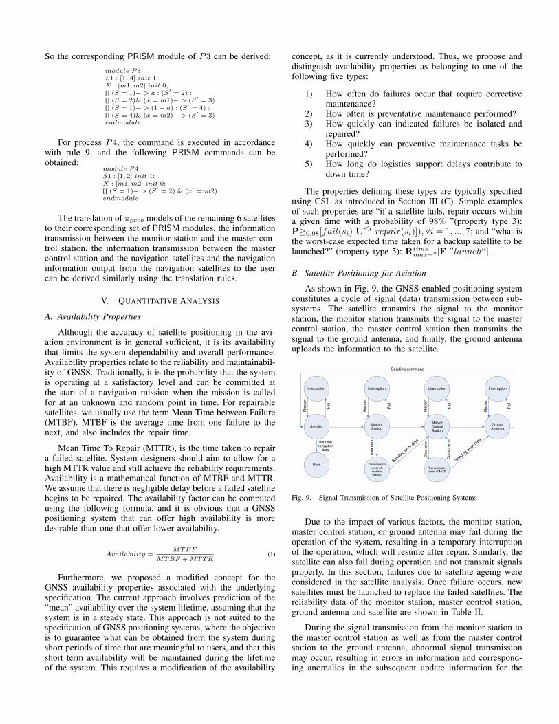
As shown in Fig. 9, the GNSS enabled positioning systemconstitutes a cycle of signal (data) transmission between sub-systems. The satellite transmits the signal to the monitorstation, the monitor station transmits the signal to the mastercontrol station, the master control station then transmits thesignal to the ground antenna, and finally, the ground antennauploads the information to the satellite.
Interruption Interruption Interruption
Monitor Station
Master Control Station
Ground Antenna
User Transmission error of monitor station
Transmission error of MCS
Interruption
Satellite
Dat
a er
ror
Sending error d
ata
Sending command
Rep
air
Rep
air
Rep
air
Rep
air
Fail
Fail
Fail
Fail
Sendingnavigation
data
Sending error d
ata
Dat
a er
ror
Cor
rect
erro
r
Fig. 9. Signal Transmission of Satellite Positioning Systems
Due to the impact of various factors, the monitor station,master control station, or ground antenna may fail during theoperation of the system, resulting in a temporary interruptionof the operation, which will resume after repair. Similarly, thesatellite can also fail during operation and not transmit signalsproperly. In this section, failures due to satellite ageing wereconsidered in the satellite analysis. Once failure occurs, newsatellites must be launched to replace the failed satellites. Thereliability data of the monitor station, master control station,ground antenna and satellite are shown in Table II.
During the signal transmission from the monitor station tothe master control station as well as from the master controlstation to the ground antenna, abnormal signal transmissionmay occur, resulting in errors in information and correspond-ing anomalies in the subsequent update information for the
TABLE II. RELIABILITY OF SPACE AND CONTROL SEGMENTS.
Systems MTBF (hours) MTTR
Satellite depends on the model 6 monthsMonitor Station 156000 25.2 minutesMaster Control Station 1248 52.3 minutesGround Antenna 2310 4.2 hours
satellites. This can affect the navigation safety of users if thesituation is severe. If anomalies occur in signal transmission,the master control station can correct the signal after a certainperiod of time.
Based on a preliminary investigation, it is assumed in ouranalysis that the information exchange among the satellites,monitor station and ground antenna does not itself generateinformation anomalies, but its reliability is a direct conse-quence of the reliabilities of the satellites and ground antenna.It is additionally assumed that information anomalies can onlyoccur in the signal transmission between the master controlstation and the monitor station. These assumptions and relateddata are based on relevant reports3 on GPS, as summarised inTable III.
TABLE III. TRANSMISSION RELIABILITY OF SEGMENTS.
Systems Transmission reliability
Satellite-Monitor Station depends on reliability of satellitesMonitor Station-Master Control Station 0.99999Master Control Station-Ground Antenna 0.99999Ground Antenna-Satellite depends on reliability of ground antennas
Where available, the data used for quantitative analysis inthis study were collected from the official published data [19].In other cases we used data for similar systems. The satellitemodels involved in the GPS satellite availability analysis ofthis section are Block-IIA, Block-IIR and Block-IIRM. ACTMC model was constructed based on the analysis of therelationships in the navigation system so that a quantitativeanalysis could be performed to check the model.
C. Preliminary Results and Discussion
Quantitative analysis was performed on the 7 satellitesinvolved in the system using the PRISM model checker. Asthe satellites are independent of each other, probabilistic modelchecking is run on each satellite separately according to itsrespective characteristics. The starting point of the analysison each satellite was the time on which the satellite waslaunched. The availability analysed is the satellites for thenavigation mission from the beginning until the end of themission. The data on the GPS satellites’ availability obtainedfrom the quantitative analysis can be shown in Table I.
The availability of various GPS satellites was greater than99.944% under the set rules. Satellites A, C, D and E werethe latest model, Block-IIRM, and had the largest availabilityfor navigation: the probability of these satellites being availablefor navigation during the mission was 99.9449%. The model ofsatellite F is Block-IIR, and its probability of being availablefor navigation during the mission was 99.9448%. The model ofsatellites B and G is Block-A, and its availability is 99.9447%.
3Global Positioning System (GPS) Performance Quarterly Report
The above results indicate that satellites of the same modelhad the same availability. Model Block-IIRM had the largestavailability for navigation, followed by Block-IIR and thenBlock-A. The availability data indicates that the navigationtime and the duration of use of a GPS satellite do not havelarge impacts on the satellite’s availability. Rather, the factorthat had the greatest effect on navigation was the design lifeand reliability of the navigation satellite.
The availability of the GPS constellation of seven satellitesare shown in Table IV, and the availability reaches 99.9448%.We are neglecting environmental factors, so our measure ofavailability to may be slightly greater than when they areincluded. An actual mission will involve multiple satellites,and each channel has multiple backup satellites. Thus, oncea failure occurs, the channel will be switched to a backupsatellite. Therefore, the availability of GNSS in practice willbe larger than that shown in our analysis. Moreover, thepresence of multiple satellites will potentially increase theoverall availability along an air line, but the increase ofavailable satellites does not necessarily guarantee an improveduser-satellites geometry due to the similar orbital arrangementof most GNSS satellites.
To validate the reliability of the evaluation data, we referredto some of the literature and official reports from the civilaviation sector. The U.S. Federal Aviation Administration(FAA) releases quarterly reports on the performance analysisof the system based on the operation of the GPS in eachquarter to ensure the navigation safety of global aviation [20].According to the monitoring reports released by the FAA,the availability of each individual GPS satellite has beenapproximately 99.96% [20]. This number is very close to thatobtained in our analysis and is in line with the estimatedvalue of this study, confirming, from one line of evidence,the feasibility and applicability of our approach.
VI. RELATED WORK
Prediction of satellite navigation availability is very usefulfor numerous applications such as airplane navigation missionsand in-car navigation systems. Simulation is nowadays widelyused to analyse performance and predicate availability fora variety of satellite systems [21]–[24]. In [21], softwaresimulation based on a Markov model of a GPS constellation of24 satellites is used to obtain availability estimates of GNSSin Taiwan. In [22], an automated method for predicting thenumber of satellites available to a GPS receiver, at any pointon the Earth’s surface at any time is described. In [23], theavailability of a navigation and communication satellite system(NCSS) is studied to examine the feasibility of using a NCSSconstellation in Australia. A performance model was proposedin [24] to evaluate the availability of satellite systems overgeographic grid averaging areas over a given period of time.
Availability characteristics for GPS and GPS augmented bygeostationary satellites (GSs) are compared in [25] . Availabil-ity is determined for users in the contiguous zone in UnitedStates, based on the planned operational GPS constellation andvarious GS deployments. In [26], a method for determining theavailability of three different GPS services (positioning, sup-plemental navigation, and sole means navigation) is describedfor both two-dimensional and three-dimensional applications.A 21-satellite and a 24-satellite constellation are considered.In the companion paper [27], state probability analyses of 21-and 24-satellite constellations based on a Markov chain modelare discussed.
VII. CONCLUSIONS AND FUTURE WORK
In this paper we present a formal approach to analyse theavailability properties of GNSS based positioning systems. Wehave modelled some aspects (e.g., communication, movement,unreliable transmission) of the system for navigating a specificflight in the probabilistic ⇡-calculus, a process algebra whichsupports modelling of concurrency, uncertainty, and mobility.Then we encode our process algebraic models into the PRISMlanguage. Finally, we analyse the availability properties thatrelate to the dependability and overall performance of theunderlying system.
Although nowadays satellite positioning is commonly usedin the aviation sector, it is still to gain a foothold in otherindustries such as the rail industry. One major barrier thatpresents its application to railway safety is the lack of evidencethat the concept and theory for the verification of railway appli-cations with introduction of GNSS is applicable based on thejoint use of aviation and railway standards and requirements.Up to now availability analysis is non-trivial because difficultsituations exist on the railways due to the limitations of theGNSS coverage in urban canyons, tunnels, and forest areas.For future work, we plan to add a fourth environment segmentthat simulates such difficult situations to the GNSS.
ACKNOWLEDGMENT
This research was partially supported by the EuropeanCommission (EC) EATS project (FP7-TRANSPORT-314219).The author Yu Lu was funded by the Scottish Informatics andComputer Science Alliance (SICSA).
REFERENCES
[1] S. Arrizabalaga, J. Mendizabal, S. Pinte, J. Sanchez, J. Gonzalez,J. Bauer, M. Themistokleous, and D. Lowe, “Development of anAdvanced Testing System and Smart Train Positioning System forETCS applications,” in Proc. 5th Transport Research Arena Conference(TRA’15), 2014.
[2] C. W. Johnson, “Innovation vs Safety: Hazard Analysis Techniquesto Avoid Premature Commitment in the Early Stage Development ofNational Critical Infrastructures,” in Proc. 32nd International SystemsSafety Conference, 2014.
[3] Y. Lu, Z. Peng, A. Miller, T. Zhao, and C. Johnson, “Timed Fault TreeModels of the China Yongwen Railway Accident,” in Proc. 8th AsiaModelling Symposium (AMS’14). IEEE, 2014.
[4] Z. Peng, Y. Lu, A. Miller, C. Johnson, and T. Zhao, “Risk assessmentof railway transportation systems using timed fault trees,” Quality andReliability Engineering International, 2014.
[5] M. Kwiatkowska, G. Norman, and D. Parker, “PRISM: ProbabilisticModel Checking for Performance and Reliability Analysis,” ACMSIGMETRICS Performance Evaluation Review, vol. 36, no. 4, pp. 40–45, 2009.
[6] R. Alur and T. A. Henzinger, “Reactive Modules,” Formal Methods inSystem Design, vol. 15, no. 1, pp. 7–48, 1999.
[7] G. Norman, C. Palamidessi, D. Parker, and P. Wu, “Model CheckingProbabilistic and Stochastic Extensions of the ⇡-Calculus,” IEEE Trans-actions on Software Engineering, vol. 35, no. 2, pp. 209–223, 2009.
[8] Y.-W. Lee, Y.-C. Suh, and R. Shibasaki, “A simulation system for GNSSmultipath mitigation using spatial statistical methods,” Computers &Geosciences, vol. 34, no. 11, pp. 1597–1609, 2008.
[9] Z. Peng, Y. Lu, A. Miller, C. Johnson, and T. Zhao, “A ProbabilisticModel Checking Approach to Analysing Reliability, Availability, andMaintainability of a Single Satellite System,” in Proc. 7th EuropeanModelling Symposium (EMS 2013). IEEE, 2013, pp. 611–616.
[10] Z. Peng, Y. Lu, A. Miller, T. Zhao, and C. Johnson, “Formal Spec-ification and Quantitative Analysis of a Constellation of NavigationSatellites,” Quality and Reliability Engineering International, 2014.
[11] R. Abo and K. Barkaoui, “A Performability Analysis of Mobile WirelessSensor Networks with Probabilistic Model Checking,” in Proc. 7thWireless Advanced (WiAd’11). IEEE, 2011, pp. 283–288.
[12] M. Hennessy and H. Lin, “Symbolic bisimulations,” Theoretical Com-puter Science, vol. 138, no. 2, pp. 353–389, 1995.
[13] M. Kwiatkowska, G. Norman, and D. Parker, “Stochastic Model Check-ing,” in Proc. 7th International Conference on Formal Methods forPerformance Evaluation (SFM’07). Springer, 2007, pp. 220–270.
[14] C. Baier, J.-P. Katoen, and H. Hermanns, “Approximative Sym-bolic Model Checking of Continuous-Time Markov Chains,” in Proc.10th International Conference on Concurrency Theory (CONCUR’99).Springer, 1999, pp. 146–161.
[15] A. Aziz, K. Sanwal, V. Singhal, and R. Brayton, “Model-CheckingContinuous-Time Markov Chains,” ACM Transactions on Computa-tional Logic, vol. 1, no. 1, pp. 162–170, 2000.
[16] E. A. Emerson, “Temporal and modal logic,” in Handbook of Theoret-ical Computer Science. Elsevier, 1990, pp. 996–1072.
[17] H. Hansson and B. Jonsson, “A Logic for Reasoning about Time andReliability,” Formal Aspects of Computing, vol. 6, no. 5, pp. 512–535,1994.
[18] R. Alur, C. Courcoubetis, and D. Dill, “Model-Checking for Real-TimeSystems,” in Proc. 5th Annual IEEE Symposium on Logic in ComputerScience (LICS’90). IEEE, 1990, pp. 414–425.
[19] W. Marquis and M. Shaw, “GPS III: Bringing New Capabilities to theGlobal Community,” Inside GNSS, pp. 34–48, September 2011.
[20] FAA, “Global Positoning System (GPS) Standard Positioning Service(SPS) Performance Analysis Report,” 2013.
[21] H.-S. Wang and P.-C. Hsiao, “GNSS Availability Analysis in Taiwan- a Markov Model Approach,” in Proc. National Technical Meeting ofION, 2006, pp. 759–769.
[22] G. Taylor, J. Li, D. Kidner, C. Brunsdon, and M. Ware, “Modellingand prediction of GPS availability with digital photogrammetry andLiDAR,” International Journal of Geographical Information Science,vol. 21, no. 1, pp. 1–20, 2007.
[23] K. Kubik, Y. Feng, and T. Tang, “An Availability Study for a Nav-ComSatellite System (NCSS) in Australia,” in Proc. 9th National SpaceEngineering Symposium, 1994, pp. 59–66.
[24] C. Kelley and M. Dessouky, “Minimizing the Cost of Availability ofCoverage from a Constellation of Satellites: Evaluation of OptimizationMethods,” Systems Engineering, vol. 7, no. 2, pp. 113–122, 2004.
[25] W. S. Phlong and B. D. Elrod, “Availability Characteristics of GPS andAugmentation Alternatives,” Navigation, vol. 40, no. 4, pp. 409–428,1993.
[26] J.-M. Durand, T. Michal, and J. Bouchard, “GPS Availability, part I:Availability of Service Achievable for Different Categories of CivilUserspart i: Availability of Service Achievable for Different Categoriesof Civil Users,” Navigation, vol. 37, no. 2, pp. 123–139, 1990.
[27] J.-M. Durand and A. Caseau, “GPS Availability, Part II: Evaluationof State Probabilities for 21 Satellite and 24 Satellite Constellations,”Navigation, vol. 37, no. 3, pp. 285–296, 1990.


![[1] H. He, J. Tian, M. Zhao, J. Xue, y K. Lu, «3D Medical ...pegasus.javeriana.edu.co/~CIS1130TK03/documentos/Anexo3... · He, J. Tian, M. Zhao, J. Xue, y K. Lu, «3D Medical Imaging](https://static.documents.pub/doc/80x56/5ad329d57f8b9a92258e0e2a/1-h-he-j-tian-m-zhao-j-xue-y-k-lu-3d-medical-cis1130tk03documentosanexo3he.jpg)


![GLU3.0: Fast GPU-based Parallel Sparse LU …arXiv:1908.00204v2 [cs.DC] 2 Aug 2019 GLU3.0: Fast GPU-based Parallel Sparse LU Factorization for Circuit Simulation Shaoyi Peng, Student](https://static.documents.pub/doc/80x56/5e70d3e0657c551f9b7856c6/glu30-fast-gpu-based-parallel-sparse-lu-arxiv190800204v2-csdc-2-aug-2019.jpg)


