Lua, Boundary Conditions and ect..

Some further informations about calculating in Femm M. Rad

27.04.2018

Outline

• Lua scripting• Border conditions• About torque and force calculation in

Femm

Lua scripts

• To automate calculation in Femm we can use Lua scripts

• Lua is a language which is used also in some other applications (eg. Adobe Photoshop Lightroom)

• More informations about the language it self you can find on: http://www.lua.org/about.html

Automating the calculations

• Almost all activities related to the calculation of the field can be written as a macro in LUA scripting language.

• This is especially useful when performing the same calculations repeatedly, for example by setting the field and force versus displacement of armature of an electromagnet.

• By the Lua scripts we can also export results in various format

• In this way, even hours of calculations can be realized automatically, for example at night. After its completion, we have access to the final results in the form of drawings or ASCII files.

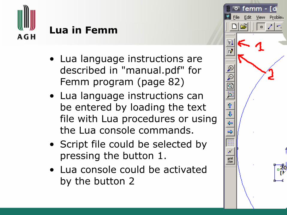
Lua in Femm

• Lua language instructions are described in "manual.pdf" for Femm program (page 82)

• Lua language instructions can be entered by loading the text file with Lua procedures or using the Lua console commands.

• Script file could be selected by pressing the button 1.

• Lua console could be activated by the button 2

Lua - how to start

• First, it is good idea to make a separate empty folder for script calculations

• It is good to remember that Lua script from file is started just after loading

• A very good practice is to perform modifications on a copy of the model instead on the initial model. For this purpose at the beginning of the script you can put eg .:open("initial_model.fem")

mi_saveas("model_automated.fem")

Model preparing

• The model for calculations using the Lua script has to be prepared firstly and tested

• Elements for modification should be assigned to one group. It helps to operate on them.

Notes on calculations

• If you are planning calculations where the transfers or turnovers are performed, it is a good idea to determine whether extreme positions of all elements are correct (eg. whether the items or materials do not overlap each other)

• This can be achieved by running the procedure with a few big steps (just to calculate at the beginning only two or three cases, but on whole range)

Sample Lua script

• in Lua:• Comments we can put

after '--'• Line is ended only by the

'enter'• Variables are defined by

giving them a value

• Functions can return a few values (not only one)

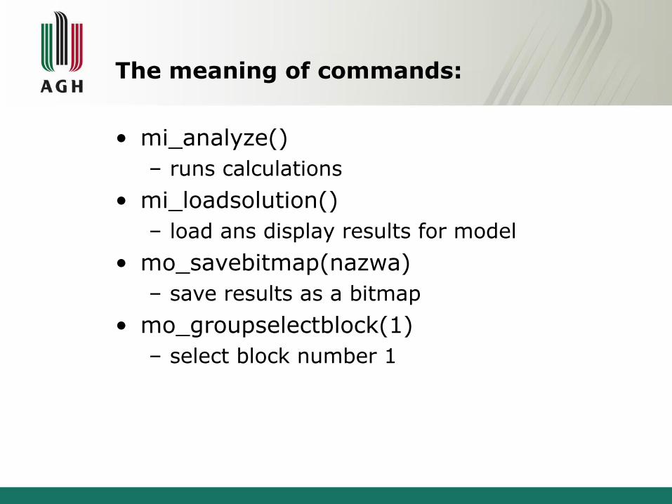
The meaning of commands:

• mi_analyze()– runs calculations

• mi_loadsolution() – load ans display results for model

• mo_savebitmap(nazwa)– save results as a bitmap

• mo_groupselectblock(1)– select block number 1

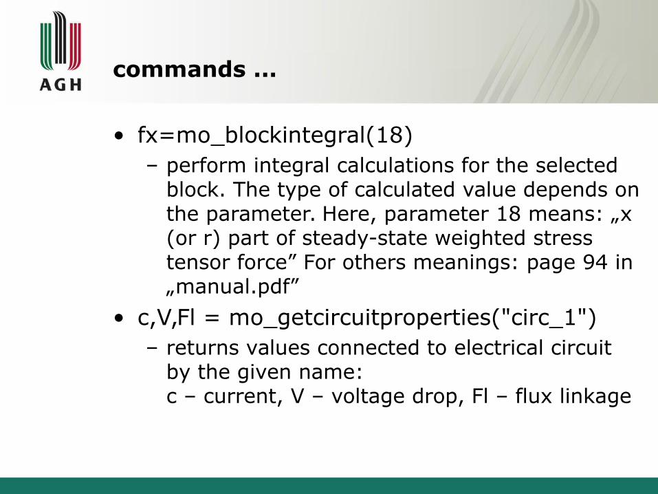
commands ...

• fx=mo_blockintegral(18)– perform integral calculations for the selected

block. The type of calculated value depends on the parameter. Here, parameter 18 means: „x (or r) part of steady-state weighted stress tensor force” For others meanings: page 94 in „manual.pdf”

• c,V,Fl = mo_getcircuitproperties("circ_1") – returns values connected to electrical circuit

by the given name: c – current, V – voltage drop, Fl – flux linkage

Commands ….

• print(shift," ",fx," ",Fl," ",V)– prints values in Lua console

• write(outfile,shift," ",fx," ",Fl," ",V,"\n")– write values to previously opened file – (variable 'outfile' is a handler to file,

returned by 'openfile(..)' function )

• mo_close()– Closes active postprocessor window (results

window)

Commands …..

• mi_seteditmode("group")– Sets the edit mode to “group” as it is in

Femm program (it could be also: "nodes", "segments", "arcsegments", "blocks", "group")

• mi_selectgroup(1)– select group number 1

• mi_movetranslate(step,0) – Move active element or group by the vector

(here the vector is (step,0))

Commands ...

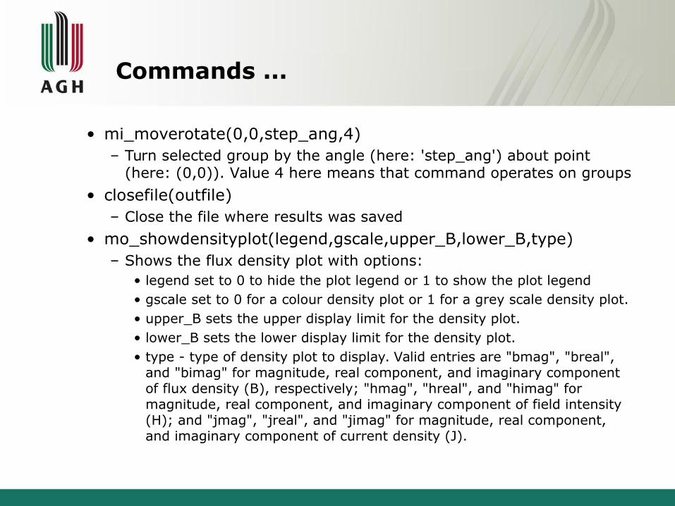
• mi_moverotate(0,0,step_ang,4)– Turn selected group by the angle (here: 'step_ang') about point

(here: (0,0)). Value 4 here means that command operates on groups

• closefile(outfile)– Close the file where results was saved

• mo_showdensityplot(legend,gscale,upper_B,lower_B,type) – Shows the flux density plot with options:

• legend set to 0 to hide the plot legend or 1 to show the plot legend• gscale set to 0 for a colour density plot or 1 for a grey scale density plot.• upper_B sets the upper display limit for the density plot.• lower_B sets the lower display limit for the density plot.• type - type of density plot to display. Valid entries are "bmag", "breal",

and "bimag" for magnitude, real component, and imaginary component of flux density (B), respectively; "hmag", "hreal", and "himag" for magnitude, real component, and imaginary component of field intensity (H); and "jmag", "jreal", and "jimag" for magnitude, real component, and imaginary component of current density (J).

Border conditions

• Finite element method can not be used for issues whose field extends to infinity.

• To be able to analyze such problems as electromagnetic field we have to limit the analysis area by the border and set imposed boundary conditions.

• To simulate on artificial border the physical phenomena occurring there in fact, the boundary procedures are used.

• Thus the analysis is limited to a given area, but the field outside of the area is also taken into account.

Border conditions, procedures

• Standard FEM method can be used only for simply connected regions - introduction of a procedure also allows us to analyze the areas which are not simply connected. For example areas with fragments which are excluded from the analysis.

Types of border conditions in Femm

• Dirichlet:In this type of boundary condition, the value of potential A or V is explicitly defined on the boundary, e.g. A = 0. The most common use of Dirichlet-type boundary conditions in magnetic problems is to define A = 0 along a boundary to keep magnetic flux from crossing the boundary. In electrostatic problems, Dirichlet conditions are used to fix the voltage of a surface in the problem domain.

Border conditions ...

• Neumann: This boundary condition specifies the normal derivative of potential along the boundary. In magnetic problems, the homogeneous Neumann boundary condition, ∂A/∂n =0 is defined along a boundary to force flux to pass the boundary at exactly a 90o angle to the boundary. This sort of boundary condition simulates an interface with a very high permeable metal.

Border conditions ...

• Robin:The Robin boundary condition is sort of a mix between Dirichlet and Neumann prescribing a relationship between the value of A and its normal derivative at the boundary. An example of this boundary condition is:

– This boundary condition is most often in FEMM to define “impedance boundary conditions” that allow a bounded domain to mimic the behavior of an unbounded region. In the context of heat flow problems, this boundary condition can be interpreted as a convection boundary condition. It means the setting the rate of spatial change of temperature just near the border which is depending on the temperature difference between the surface and the environment.

∂ A∂ n

+cA=0

Border conditions ...

Periodic,• A periodic boundary conditions joins two

boundaries together. In this type of boundary condition, the boundary values on corresponding points of the two boundaries are set equal to one another.

Border conditions ...

Antiperiodic• The antiperiodic boundary condition also

joins together two boundaries. However, the boundary values are made to be of equal magnitude but opposite sign.

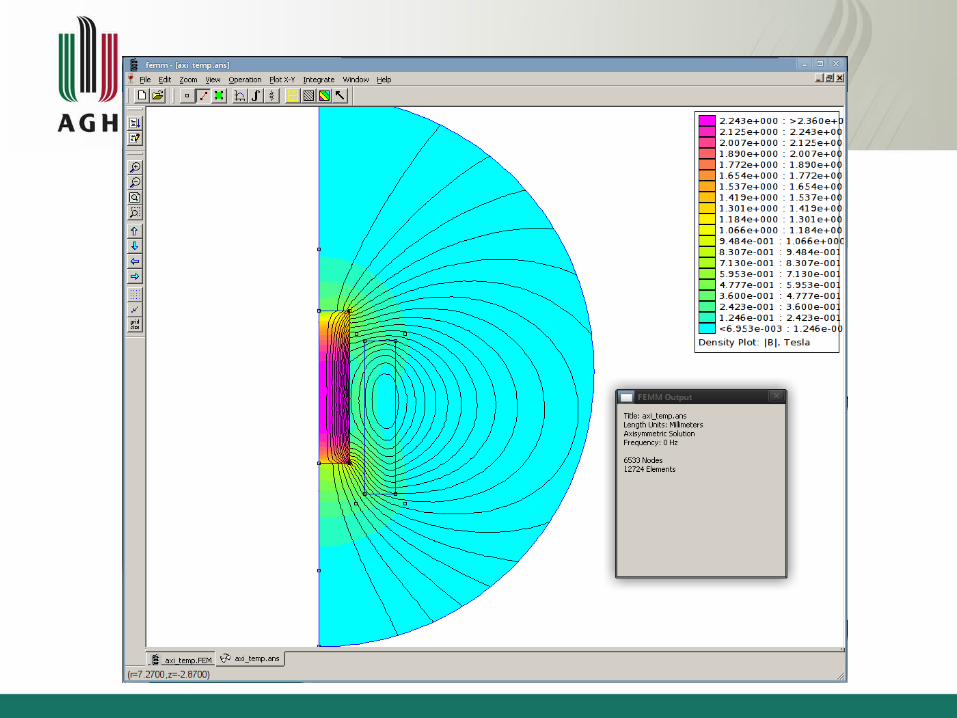
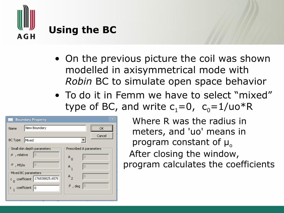
Using the BC

• On the previous picture the coil was shown modelled in axisymmetrical mode with Robin BC to simulate open space behavior

• To do it in Femm we have to select “mixed” type of BC, and write c1=0, c0=1/uo*R– Where R was the radius in

meters, and 'uo' means in program constant of μo

After closing the window, program calculates the coefficients

Calculating the forces in Femm

• Lorentz Force/TorqueIf we want to compute the force on a collection of currents in a region containing only materials with a unit relative permeability, the volume integral of Lorentz torque is always the method to employ. Lorentz force results tend to be very accurate. However, again, they are only applicable for the forces on conductors of with unit permeability (e.g. coils in a voice coil actuator).F = B*I*l*sin(α)

Force calculating

• Weighted Stress Tensor Volume IntegralThis volume integral greatly simplifies the computation of forces and torques, as compared to evaluating forces via the stress tensor line integral of differentiation of coenergy. Merely select the blocks upon which force or torque are to be computed and evaluate the integral. No particular “art” is required in getting good force or torque results although results tend to be more accurate with finer meshing around the region upon which the force or torque is to be computed.

• One limitation of the Weighted Stress Tensor integral is that the regions upon which the force is being computed must be entirely surrounded by air. In cases in which the desired region abuts a non-air region, force results may be deduced from differentiation of Coenergy

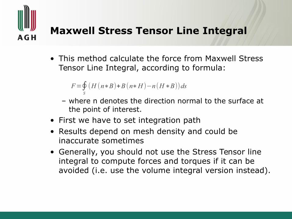
Maxwell Stress Tensor Line Integral

• This method calculate the force from Maxwell Stress Tensor Line Integral, according to formula:

– where n denotes the direction normal to the surface at the point of interest.

• First we have to set integration path• Results depend on mesh density and could be

inaccurate sometimes • Generally, you should not use the Stress Tensor line

integral to compute forces and torques if it can be avoided (i.e. use the volume integral version instead).

F=∮S

(H (n∗B)+B (n∗H )−n (H∗B))ds

Frequency setting in problem definition

• Default value is 0. • If we put another value ALL field values

will alternate with this frequency• Therefore mixing problems with permanent

magnet and frequency given do not lead to the sensible results

Eddy currents

• Femm can simulate eddy currents in materials with non zero conductivity.

• It assumes that all regions where the eddy currents may be inducted are connected in “infinity”

• If we want to avoid this, we can set the parallel circuits with zero current, which are connected similar to the real case.

Some parts are based on “manual.pdf”: Finite Element Method Magnetics

Version 4.2User’s Manual

August 25, 2013