LuanFilipedosSantosColombari AnApproachtoHandleSuddenLoad ... - Biblioteca Digital de ... · 2017....

University of São Paulo–USPSão Carlos School of Engineering

Department of Electrical and Computing EngineeringElectrical Engineering Graduate School

Luan Filipe dos Santos Colombari

An Approach to Handle Sudden LoadChanges on Static Voltage Stability

Analysis

São Carlos2017

Luan Filipe dos Santos Colombari

An Approach to Handle Sudden LoadChanges on Static Voltage Stability

Analysis

Master Thesis presented to the Electrical En-gineering Graduate School of the São CarlosSchool of Engineering to achieve the require-ments to obtain the title of Master of Science.

Field of Research: Electric Power Systems

Advisor: Rodrigo Andrade Ramos

São Carlos2017

This is the final corrected version of this masters dissertation. The original version is available inEESC/USP where the respective Electrical Engineering Graduate School is located.

AUTORIZO A REPRODUÇÃO TOTAL OU PARCIAL DESTE TRABALHO,POR QUALQUER MEIO CONVENCIONAL OU ELETRÔNICO, PARA FINSDE ESTUDO E PESQUISA, DESDE QUE CITADA A FONTE.

Colombari, Luan Filipe dos Santos C718a An approach to handle sudden load changes on static

voltage stability analysis / Luan Filipe dos SantosColombari; orientador Rodrigo Andrade Ramos. SãoCarlos, 2017.

Dissertação (Mestrado) - Programa de Pós-Graduação em Engenharia Elétrica e Área de Concentração emSistemas Elétricos de Potência -- Escola de Engenhariade São Carlos da Universidade de São Paulo, 2017.

1. Electric Power Systems. 2. Voltage Stability. 3. Continuation Power Flow. 4. Distributed Generation. 5.Undervoltage Load Shedding. I. Título.

To my father, Carlos Colombari, who sadly had to pass away to be awarded with thismodest recognition. He was one of the smartest men I have ever met and didn’t even know

what a master thesis is.

Acknowledgments

In special, I thank Prof. Rodrigo Andrade Ramos, for advising this dissertation andcontributing to my development as a researcher, a professional and a future professor.

Acknowledgments to CNPq (National Counsel of Technological and Scientific Develop-ment) for awarding me the grant 130750/2015-8.

Also, I thank my mother, Maria Clélia dos Santos, for supporting me emotionally andfinancially during my master studies.

I’m greatly thankful for my soon to be wife, Camila Silva Vieira, for her kindness,patience and understating, specially regarding the hours and weekends required to finishthis research.

I am in huge debt to my friend Fabrício Mourinho for all the professional and personalhelp provided all over the years. Particularly, to get in this graduate program and tolend me his house in the beginning of my master studies. For this last support, I thankRodolpho Neves, Breno Carvalho and Renzo Bastos as well.

Thanks to Prof. Roberto Lotero for his several contributions in my academic careerand personal life.

I also thank my friend and roommate Mohamad Ismail for all the help and companion-ship. Furthermore, thanks to Marina Carvalho for her patience and understanding withmy constant intrusion in her apartment.

Finally, thanks to my laboratory colleagues, William Pereira, Marcelo Santana, EdsonGeraldi, Thales Almeida, Tatiane Fernandes, Jhonatan Andrade, Allan Gregori, AnnaMoraco, Marley Tavares, Carlos de Oliveira, Artur Piardi, Geyverson de Paula, RafaelBorges, Murilo Bento and Paulo Ubaldo. Without them this work would probably havebeen accomplished faster, however it would also have been tedious and wearisome.

“Don’t Panic”(Douglas Adams)

Abstract

Colombari, Luan Filipe dos Santos An Approach to Handle Sudden LoadChanges on Static Voltage Stability Analysis. 134 p. Master Thesis – São CarlosSchool of Engineering, University of São Paulo, 2017.

In the context of static Voltage Stability Assessment (VSA), as the power systemload grows, bus voltages tend to drop. This reduction may lead to generator or loaddisconnections caused by undervoltage protection schemes. These events comprise suddenparametric variations that affect the equilibrium diagram and the Voltage Stability Margin(VSM) of power systems. Practical examples of such sudden load changes are caused by themandatory disconnection of Distributed Generation (DG) units and Undervoltage LoadShedding (ULS). There are no thorough studies in the literature concerning these loadparametric variations and the discontinuities that they cause in power system equilibria.This dissertation describes a predictor/corrector scheme specifically designed to handlethese discontinuities, so it is possible to evaluate their effect on the VSM of power systems.This method successively calculates the load discontinuities that exist in the equilibriumlocus of the system under analysis. It results in the sequence of sudden load variationsthat happens and their overall impact on the system. When applied to quantify theeffect of DG mandatory disconnections and ULS, the proposed predictor/corrector schemeyielded better results than the traditional Continuation Power Flow (CPFLOW), whichexperienced convergence problems caused by the discontinuities under analysis. However,due to its design, the applicability of the proposed method should be restricted to powersystems that go through several successive sudden load changes. In this sense, it shouldnot be regarded as a replacement for the CPFLOW, but rather as a technique that couldaward this traditional VSA tool with new features to enhance its performance.

Keywords: Electric Power Systems; Voltage Stability; Continuation Power Flow; Dis-tributed Generation; Undervoltage Load Shedding.

Resumo

Colombari, Luan Filipe dos Santos Abordagem para Considerar Variações Súbi-tas de Carga na Análise Estática de Estabilidade de Tensão.. 134 p. Dissertaçãode mestrado – Escola de Engenharia de São Carlos, Universidade de São Paulo, 2017.

No contexto de análise estática de estabilidade de tensão, conforme a carga de umsistema de potência cresce, as tensões nas suas barras tendem a cair. Essa redução podecausar a desconexão de geradores e cargas devido a atuação de proteções de subtensão.Esses eventos representam variações abruptas de demanda que alteram o diagrama deequilíbrio de um sistema e sua Margem de Estabilidade de Tensão (MET). Exemplospráticos dessas variações são causados pelo desligamento mandatório de unidades deGeração Distribuída (GD) e pelo Corte de Carga por Subtensão (CCS). Não há estudosdetalhados na literatura que trabalham especificamente com essas variações nos parâmetrosda carga, nem com as descontinuidades que elas causam no diagrama de equilíbrio desistemas de potência. Essa dissertação descreve um procedimento especificamente projetadopara lidar com essas descontinuidades, de modo que seja possível avaliar seu efeito naMET de sistemas elétricos. Esse método calcula sucessivamente as descontinuidadesde carga que existem no diagrama de equilíbrio do sistema em análise. Ele resulta nasequência de variações súbitas de carga que ocorre e no seu impacto no sistema. Quandoo método foi aplicado para quantificar o efeito do desligamento mandatório de GD e doCCS, ele apresentou resultados melhores do que o tradicional Fluxo de Carga Continuado(CPFLOW), o qual sofreu problemas de convergência causados pelas descontinuidades emquestão. Entretanto, devido ao seu projeto, o método proposto só deve ser utilizado parasistemas de potência que estão sujeitos a várias sucessivas variações abruptas de carga. Poressa razão, esse método não pode ser considerado um substituto do CPFLOW, mas simcomo uma técnica capaz de agregar novas funcionalidades a essa ferramenta tradicional,amentando assim seu horizonte de aplicações.

Palavras-chave: Sistemas Elétricos de Potência; Estabilidade de Tensão; Fluxo de CargaContinuado; Geração Distribuída; Corte de Carga por Subtensão.

Acronyms

CAISO California Independent System OperatorCPFLOW Continuation Power FlowDG Distributed GenerationEPS Electric Power SystemLIB Limit Induced BifurcationMLP Maximum Loadability PointOLTC On-load Tap ChangerPCC Point of Common CouplingSIB Structure Induced BifurcationSNB Saddle-Node BifurcationULS Undervoltage Load SheddingVSA Voltage Stability AssessmentVSM Voltage Stability Margin

Contents

1 Introduction 191.1 Objectives . . . . . . . . . . . . . . . . . . . . . . . . . . . . . . . . . . . 211.2 Dissertation Structure . . . . . . . . . . . . . . . . . . . . . . . . . . . . . 22

2 Static Voltage Stability Analysis 232.1 Static Voltage Stability Fundamentals . . . . . . . . . . . . . . . . . . . . 252.2 Loading Parameter 𝜆 and the Load Growth Direction . . . . . . . . . . . 302.3 Continuation Power Flow (CPFLOW) . . . . . . . . . . . . . . . . . . . . 31

2.3.1 Parametrization . . . . . . . . . . . . . . . . . . . . . . . . . . . . 322.3.2 Prediction . . . . . . . . . . . . . . . . . . . . . . . . . . . . . . . 342.3.3 Correction . . . . . . . . . . . . . . . . . . . . . . . . . . . . . . . 362.3.4 Step-Length Control . . . . . . . . . . . . . . . . . . . . . . . . . . 372.3.5 CPFLOW Implementation and Evolution . . . . . . . . . . . . . . 382.3.6 Convergence Problems of the CPFLOW . . . . . . . . . . . . . . . 40

2.4 Q-limit Guided CPFLOW Proposed by Yorino et al. (2005) . . . . . . . . 422.4.1 Prediction . . . . . . . . . . . . . . . . . . . . . . . . . . . . . . . 422.4.2 Correction . . . . . . . . . . . . . . . . . . . . . . . . . . . . . . . 442.4.3 Identification of Structure Induced Bifurcation . . . . . . . . . . . 442.4.4 Implementation and General Aspects of the Method Proposed by

Yorino et al. (2005) . . . . . . . . . . . . . . . . . . . . . . . . . . 472.5 Final Remarks . . . . . . . . . . . . . . . . . . . . . . . . . . . . . . . . . 48

3 Sudden Load Variations on Static Voltage Stability Analysis 493.1 PV Curve Discontinuities Produced by Sudden Load Variations . . . . . . 513.2 Proposed Predictor/Corrector Scheme to Handle Sudden Load Variations 56

3.2.1 Load Switching Prediction . . . . . . . . . . . . . . . . . . . . . . 573.2.2 Correction Stage I - Pre Load Switching . . . . . . . . . . . . . . . 583.2.3 Correction Stage II - Post Load Switching . . . . . . . . . . . . . . 59

3.2.4 Identifying the Maximum Loadability Point (MLP) and BifurcationType . . . . . . . . . . . . . . . . . . . . . . . . . . . . . . . . . . 63

3.2.5 Complete Iterative Predictor/Corrector Scheme to Handle SuddenLoad Variations . . . . . . . . . . . . . . . . . . . . . . . . . . . . 67

3.3 Example of Application for the Proposed Predictor/Corrector Scheme . . 683.4 Final Remarks . . . . . . . . . . . . . . . . . . . . . . . . . . . . . . . . . 71

4 Case Study on Distributed Generation Mandatory Disconnection 734.1 Distribution System Model with DG for Voltage Stability Assessment of

Transmission Systems . . . . . . . . . . . . . . . . . . . . . . . . . . . . . 764.2 Numerical Results . . . . . . . . . . . . . . . . . . . . . . . . . . . . . . . 78

4.2.1 IEEE 118 bus test system . . . . . . . . . . . . . . . . . . . . . . . 804.2.2 107 bus reduced interconnected Brazilian test system . . . . . . . 88

4.3 Final Remarks . . . . . . . . . . . . . . . . . . . . . . . . . . . . . . . . . 94

5 Case Study on Dispersed Undervoltage Load Shedding 955.1 Decentralized Undervoltage Load Shedding Model . . . . . . . . . . . . . 985.2 Numerical Results . . . . . . . . . . . . . . . . . . . . . . . . . . . . . . . 98

5.2.1 IEEE 118 bus test system . . . . . . . . . . . . . . . . . . . . . . . 1005.2.2 107 bus reduced interconnected Brazilian test system . . . . . . . 105

5.3 Final Remarks . . . . . . . . . . . . . . . . . . . . . . . . . . . . . . . . . 108

6 Conclusion 111

Bibliography 113

Appendices 119

APPENDIX A IEEE 118 Bus Test System 121

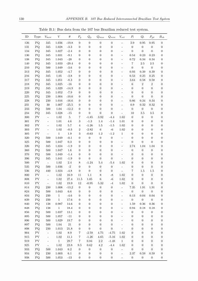
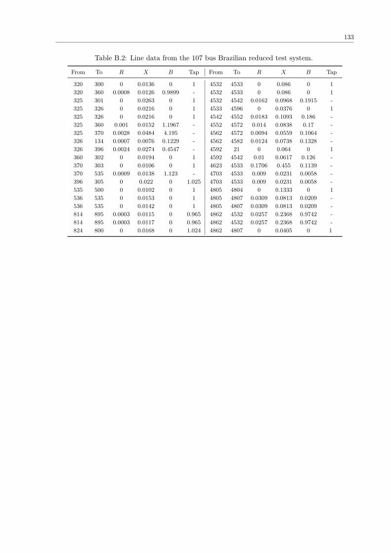
APPENDIX B 107 Bus Reduced Interconnected Brazilian Test System 129

19

Chapter 1Introduction

For several years, investments in Electric Power Systems (EPSs) were made based on aeconomy of scale paradigm, where the increasing load demand was met by the constructionof big generating facilities and long transmission lines. This scenario resulted in theinterconnected bulk power systems of nowadays. In the last few decades, environmentaland economical constraints obstructed this policy reducing drastically the investmentsin sizeable Electric Power System (EPS) expansion projects. As a consequence of that,power systems began to operate close to their operational limits (KUNDUR, 1994; CUTSEM;

VOURNAS, 2003; GAO; KUNDUR; MORISON, 1996).This scenario resulted in conditions that may lead to voltage instability in EPSs. This

phenomenon is characterized by appreciable rise or drop in bus voltages magnitudes. Incritical situations, these events may cause trip of several power system equipment and evenoriginate blackouts (CUTSEM; VOURNAS, 2003; GAO; KUNDUR; MORISON, 1996; KUNDUR

et al., 2004). An example of voltage instability was seen in Brazil in 2009, when the threetransmission lines that connect Itaipu power plant to the southeast region of the countrywere disconnected. This disturbance caused voltage sags in the state of São Paulo, whichwas responsible for the trip of the direct current transmission link between Brazil andParaguay. As a result of this succession of events, the interconnected Brazilian networkbecame unable to supply 40% of its total load in 18 different federation states (ONS, 2009).

To avoid possible load shedding caused by voltage instability, power system utilitiesare interested in such phenomena during the planning and operation of their network(MANSOUR; ALBERTO; RAMOS, 2015; LI et al., 2014; CHIANG; WANG; FLUECK, 1997).

When time domain simulations are employed to assess the voltage stability of EPSs,they require high computational effort. This may interfere with their utilization in realtime applications or situations that require the analysis of a multitude of scenarios (GAO;

KUNDUR; MORISON, 1996; BIJWE; KOTHARI; KELAPURE, 2000). Time domain simulationsexamine the dynamic behaviour of the system based on detailed models of generators,compensators and loads, as well as their associated control loops and protection schemes(VAN CUTSEM et al., 2015).

20 Chapter 1. Introduction

A practical alternative to dynamic analysis comprises static techniques employing thepower flow problem formulation. The goal of these methods is to identify the maximumcapability of the EPS to supply the power demand. This corresponds to the MaximumLoadability Point (MLP) of the system, which is the highest load level where the powerflow equations can be solved. Beyond this point there is no available stable equilibriumfor the power system to operate (CANIZARES; ALVARADO, 1993; CHIANG et al., 1995; CAO;

CHEN, 2010). Static techniques do not depict the behavior of the EPS as accurately as thedynamic ones, however they are computationally faster, which promotes their utilization inreal time applications and situations that require the analysis several EPS configurations(GAO; KUNDUR; MORISON, 1996; BALU et al., 1992; ZHAO et al., 2015).

The goal of static analysis is to assess whether there is an adequate stable equilibriumpoint for the EPS to operate with a given topology. Generally, this is assessed augmentingthe load until there is no available power flow solution. What results from this procedureis the bus voltage profiles as the load increases, which consist in the equilibrium diagramsknown as PV curves. The nose of the PV curve corresponds to the MLP of the systemunder analysis (CHIANG et al., 1995; NETO; ALVES, 2010; MANSOUR; ALBERTO; RAMOS,2015; LI et al., 2014).

A reliable and standard technique to trace EPS equilibrium diagrams and to estimatetheir MLP is the Continuation Power Flow (CPFLOW). In essence, this method solvesthe power flow equations several times as the load grows, tracing the PV curves of thesystem for a given load growth direction (CHIANG et al., 1995; AJJARAPU, 2007; CANIZARES;

ALVARADO, 1993; ALVES et al., 2000; MOLZAHN; LESIEUTRE; CHEN, 2013; SUNDHARARAJAN

et al., 2003).During the CPFLOW execution, as the load increases, some EPS devices may suddenly

change their parameters according to the system states. Examples of such equipmentare On-load Tap Changer Transformers (OLTCs), switchable shunt capacitors, excitationlimiters of generators and Undervoltage Load Shedding (ULS) protection schemes (XU;

WANG; AJJARAPU, 2012). These devices are responsible for sudden parametric changes inpower systems that, in turn, cause discontinuities in its equilibrium diagram. As a resultof them, the PV curves are not smooth nor continuous anymore, as intuitively expected.

Out of the possible parametric discontinuities that may happen in EPSs, this disserta-tion will focus on sudden load variations caused by undervoltage protection schemes. Theseare of particular interest because they can cause very severe discontinuities in PV curves,impacting significantly the voltage profile and the MLP of power systems.

Practical examples of sudden load variations that will be dealt is this dissertation com-prise Undervoltage Load Shedding (ULS) and the mandatory disconnection of DistributedGeneration (DG) units.

The mandatory disconnection of DG comprises the trip of these units caused byprotection schemes designed by distribution utilities to mitigate possible adverse effects

1.1. Objectives 21

that they may have in the network. When assessing the static voltage stability of EPSs,as the load grows, the bus voltages are expected to fall. The voltage drop may reach levelsthat could cause pick-up of DG undervoltage protections and consequently lead to theirtrip. This is equivalent to suddenly stepping load up, which may reduce the MLP andeven cause instability (WALLING; MILLER, 2002; CHEN; MALBASA; KEZUNOVIC, 2013).

Opposed to the disconnection of DG units, the ULS is responsible to increase the powersystem MLP. It sheds specific power loads, so the network is capable to supply criticalconsumers and expensive manufacturing processes. It is a last resource but an effectivemethod to assure that voltage collapse does not happen (AMRAEE et al., 2007; LEFEBVRE;

MOORS; CUTSEM, 2003; AFFONSO et al., 2004).The numerical results of this dissertation will focus on these two types of sudden load

variations. Nevertheless, the discussions presented here should not be restricted to them,being general to load parametric discontinuities.

In this context, this dissertation will address two main topics: (i) the effect of sud-den load changes in the MLP of power systems and (ii) the impact of the equilibriumdiscontinuities caused by them in the performance of the CPFLOW.

Remarkable works dealing directly with possible discontinuities in EPS equilibriumdiagrams were done by Xu, Wang and Ajjarapu (2012), Yorino, Li and Sasaki (2005).However, their analysis were restricted to reactive power limits of generators and switchableshunt capacitors. These papers and further bibliography regarding this field of researchwill be presented throughout the dissertation alongside with important theoretical conceptsthat will assist the understanding of the reader.

At this point, it is essential to point out that, to the extent of the author’s knowledge,there is no thorough work in the literature dealing with the effects of load discontinuitieson EPS equilibrium diagrams nor their influence on the performance of the continuationpower flow.

1.1 Objectives

In face of this gap, the research objectives of this dissertation are:

1. Investigate the nature of the EPS equilibrium diagram discontinuities caused bysudden parametric variations in the load.

2. Evaluate the adequacy of the CPFLOW to account for sudden parametric variationsin the load during its execution.

3. Quantify the impact of sudden parametric variations in the load on the MLP ofelectric power systems.

4. Propose a method specifically designed to account for sudden parametric variationsin the load during the MLP estimation under a static voltage stability framework.

22 Chapter 1. Introduction

1.2 Dissertation Structure

In order to demonstrate the fulfillment of these objectives, this dissertation is dividedinto 5 other chapters:Chapter 2: It presents basic concepts regarding static voltage stability assessment, along-

side with the Continuation Power Flow (CPFLOW), which is the standard methodin this field of research. Afterwards, it describes a variation of the CPFLOW to finddiscontinuities in PV curves.

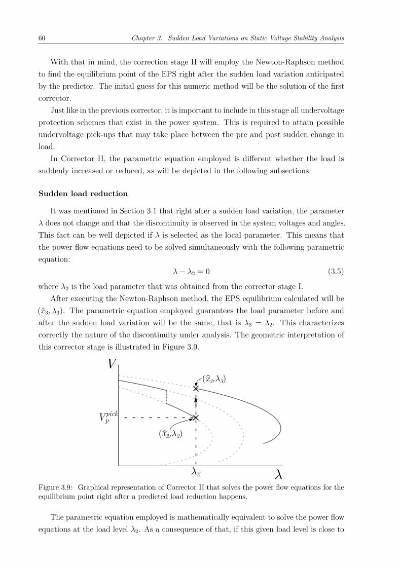
Chapter 3: It qualitatively depicts the effect of sudden load variations in the equilibriumdiagram of electric power systems. This leads to the description of a method designedto handle such parametric changes during voltage stability assessment.

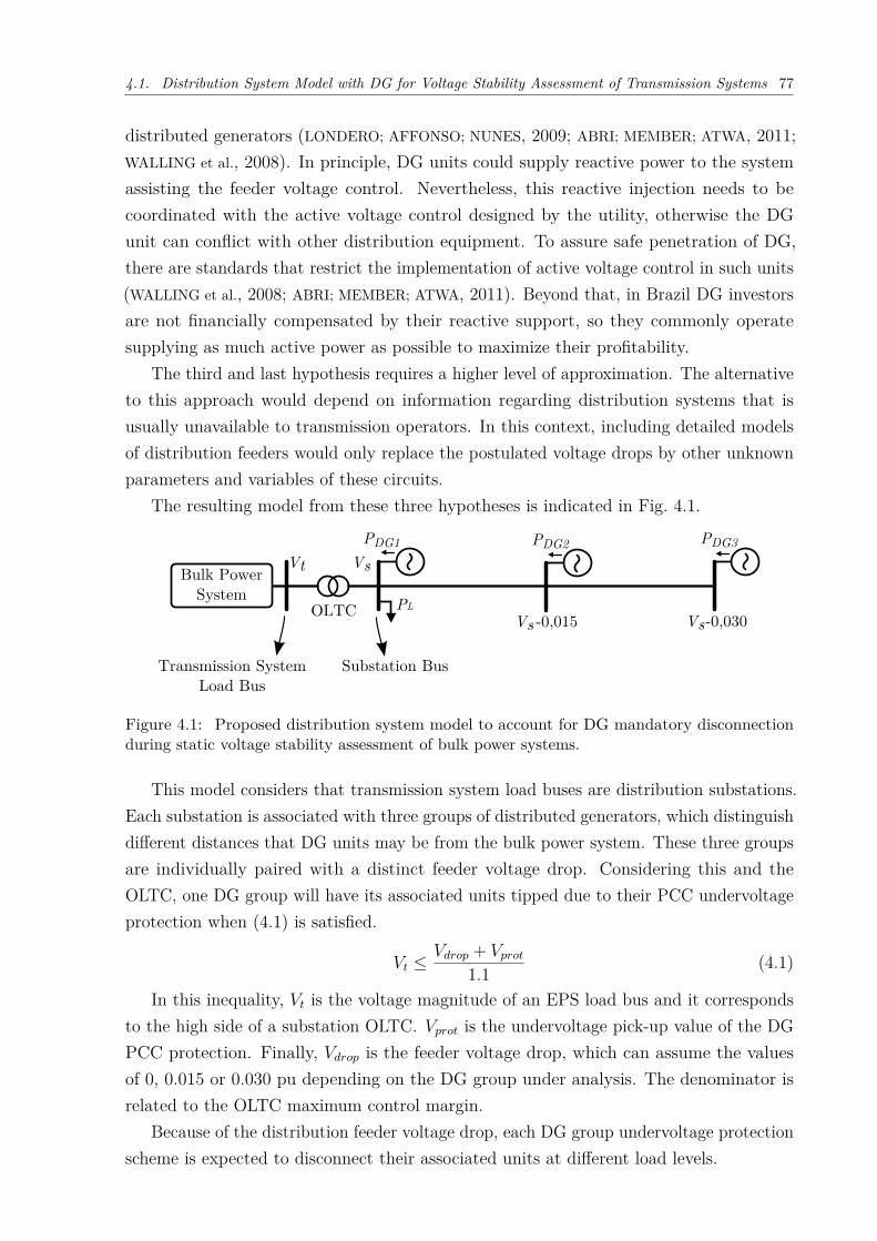
Chapter 4: Numerical results are given to illustrate the effect of DG mandatory discon-nections on the MLP of electric power systems.

Chapter 5: This time, the numerical results comprise the effect of Undervoltage LoadShedding (ULS) on the MLP of electric power systems.

Chapter 6: It presents the final conclusions of this work and possible future researchthat it could lead to.

23

Chapter 2Static Voltage Stability Analysis

Both Kundur et al. (2004) and Anderson and Fouad (2002) define voltage stabilityas the EPS ability to sustain steady bus voltages before and after the system is subjectto perturbations. Under this definition, voltage instability can be characterized by anunbounded voltage increase or reduction throughout the power system, that can lead toshut down of generators, transmission line disconnections and load shedding. In extremecases, the power system may suffer with severe small bus voltages, cascading equipmentoutages and even blackouts. Phenomenon that is known as voltage collapse (KUNDUR et

al., 2004).In a EPS, instability phenomena may happen in a multitude of scenarios with different

devices involved. As a consequence of that, it is useful to classify voltage stability accordingto the size of the disturbance under analysis and the time scale involved. Such classificationis indicated in Figure 2.1.

Voltage

stability

Small

disturbance

Large

disturbance

Short

term

Long

term

Figure 2.1: Classification of voltage instability phenomena.

Both classifications regarding disturbance size can be analysed in the two time framesmentioned. For example, it is possible to assess short and long term voltage stability aftera small disturbance. Each voltage stability category is described briefly below:

24 Chapter 2. Static Voltage Stability Analysis

Large disturbance voltage stability: It is the EPS ability to keep steady bus voltagesafter large disturbances such as severe faults, generator trips or critical transmissionline disconnections. It depends strongly on the non-linear behavior of power systemsand it should include dynamic models of loads and generators as well as protectionsettings and feedback control loops (KUNDUR et al., 2004).

Small disturbance voltage stability: It is related to the EPS ability to maintainsteady voltages after small power injection variations or following a unimportantequipment disconnection. In most cases it allows the linearisation of the powersystem dynamic model (KUNDUR et al., 2004).

Short term voltage stability: It can be associated with the dynamic response of theEPS a few seconds after a disturbance. It depends on fast acting devices such asinduction motors, electronically controlled loads and HVDC converters (CUTSEM;

VOURNAS, 2003; KUNDUR et al., 2004).Long term voltage stability: It is related to slow power system elements like On-

load Tap Changer (OLTC), thermostatically controlled loads and generator currentlimiters. In this case, the goal is to assess the system behavior several minutesfollowing a perturbation to identify situations where instability is a consequence ofequipment outages and not the disturbance itself (KUNDUR et al., 2004).

Keeping in mind this classification, voltage stability can be assessed with differenttechniques. Static voltage stability analysis is characterized by the existence of stablepower system equilibrium points after one of its parameters change. Commonly, increase ofload is the parametric variation selected for such purpose. In this scenario, the total systempower demand may reach values to which there is no stable equilibrium point available.The maximum total power that still have such point is called Maximum LoadabilityPoint (MLP) (CUTSEM; VOURNAS, 2003; AJJARAPU, 2007; CANIZARES; ALVARADO, 1993).In this situation, static voltage stability analysis is related to the existence of stableequilibrium points for the power system to operate when it is subject to successive, smalland slow load increments. In this analysis, instability is determined by the unavailabilityof a stable operating point (KUNDUR et al., 2004). Regarding the classification describedabove, static stability analysis assess the small disturbance voltage stability of a EPS inthe long term.

Static voltage stability assessment is unfit to account for several dynamic aspects ofpower systems that could cause instability. Those scenarios would require time domainsimulations of detailed dynamic models of power system equipment. When opposed to statictechniques, dynamic tools are capable to examine the transition path between differentequilibria and not simple appraise their stability feature. They can depict more accuratelyEPSs behavior, including their limiters, protections and controls (GAO; KUNDUR; MORISON,1996). For this reason, dynamic stability analysis can identify instability situations thatcould be overlooked by static techniques. Therefore, the MLP estimated with static

2.1. Static Voltage Stability Fundamentals 25

applications should be regarded as an optimistic result (BIJWE; KOTHARI; KELAPURE,2000; SAUER; PAI, 1990).

Despite being more accurate, dynamic analysis require high computational effort andsimulation time. This makes it inadequate for applications that require stability assessmentof several EPS configurations, which is the case of contingency screening and ranking(MANSOUR, 2013; BALU et al., 1992; GAO; KUNDUR; MORISON, 1996). In this circumstance,static tools are employed to identify critical configurations that would require furtherdynamic stability assessment. This means that this two techniques do not compete witheach other and their utilization should be complementary and not exclusive (BIJWE;

KOTHARI; KELAPURE, 2000).Two engineering practice examples are given to demonstrate the relevance of static

voltage stability analysis in electric power systems. Both the California IndependentSystem Operator (CAISO) and the Brazilian System National Operator (ONS - OperadorNacional do Sistema) employ static simulations to assure safe operation of their respectivesystem (LI et al., 2014; ONS, 2011).

This chapter will discuss basic concepts regarding static voltage stability analysis ofbulk power systems in Section 2.1. Next, in Section 2.2, a load growth parametrizationtechnique is described. Such formulation is indispensable to use the standard voltagestability assessment tool known as CPFLOW that is presented in Section 2.3. In Section2.4, a method proposed by Yorino, Li and Sasaki (2005) to find equilibrium discontinuitiescaused by reactive limits of generators is described. This method is included here becauseit is a key reference dealing directly with PV curve discontinuities and it will be the basisof the study done in this dissertation regarding sudden load changes. Finally, the finalremarks of the chapter are presented in section 2.5.

2.1 Static Voltage Stability Fundamentals

For stability analysis, power systems are generally modeled as a non-linear dynamicsystem described with a set of dynamic and algebraic equations (CUTSEM; VOURNAS, 2003;SAUER; PAI, 1990).

˙𝑥 = h(��, 𝑦)0 = g(��, 𝑦)

(2.1)

where �� and 𝑦 are the vectors containing, respectively, the states and algebraic variablesof the power system.

During static analysis the goal is to calculate equilibrium points of this dynamic model,which means solving (2.1) for the power system states when ˙𝑥 is equal to zero. Aftercalculating an equilibrium, it is still indispensable to determine whether or not such pointis stable. For this purpose it is possible to employ the Hartman–Grobman theorem, whichguarantees that the stability characteristic of one equilibrium point can be determined from


the eigenvalues of the linearised dynamic system at this point. If none of its eigenvalueshave positive or zero real part, then the this solution is said to be stable (CHICONE, 1999).As a consequence of the linearisation procedure, that is to say that the Jacobian of (2.1)evaluated at the given equilibrium define the power system stability around such point.

A simplification of this process commonly used in voltage stability assessment is toneglect the dynamic equations of the EPS and to consider that the traditional power flowformulation is enough to represent power system equilibrium points (CAO; CHEN, 2010;SAUER; PAI, 1990; KUNDUR et al., 2004; ZHAO et al., 2015; MANSOUR, 2013). From thisapproximation power flow solutions represent the bulk system steady state points and theJacobian of such equations establish their stability.

Even though the power flow equations are contained in the algebraic set g(��, 𝑦), theyalone are not enough to represent the non-linear dynamic system that model EPS (SAUER;

PAI, 1990). Still, power flow techniques are well established in the power system industryas a dependable tool to evaluate steady state characteristics and they will be used in thisdissertation to define power system equilibrium points.

The power flow problem can be written in the following compact form:

0 = f(𝑉 , 𝜃) + 𝜆�� (2.2)

where 𝑉 and 𝜃 are the vectors of bus voltages magnitudes and angles. The dimensionof both these vectors is equal to the number of buses (𝑛𝑏) of the power system underanalysis. Besides that, 𝜆 is a scalar that represents the loading level, as it increases sodoes the system total demand. Vector �� defines the load growth direction. This meansthat it indicates at which buses this increase takes place and at which rate it happens. Itsdimension is equal to twice the number of buses (2 · 𝑛𝑏), since there it has one componentfor the active and reactive power injection in each bus.

Varying the load parameter 𝜆 and solving the power flow equations, it is possible todraw the EPS equilibrium diagram when the load grows in direction ��. This results in thediagram known as PV curve or nose curve that depicts the system bus voltage variationas the load increases. A qualitative example of a PV curve is shown in Figure 2.2.

Investigating the power flow Jacobian eigenvalues, it is possible to conclude thatthe upper portion of the PV curve comprises stable equilibrium points, while the lowerportion contains unstable ones. The latter can be associated with a single eigenvaluewith positive real component. The PV curve nose represent the power system MaximumLoadability Point (MLP). If the system actual load is bigger than this value, then there isno equilibrium point for the system to operate resulting in instability.

The MLP is directly related to the capability of the transmission lines to deliver powerand with the ability of the generators to supply the reactive power demanded by thenetwork and the loads (LI et al., 2014; KUNDUR et al., 2004).


Stable

Equilibria

V

P

Curve

Nose (MLP)

Vcrit

Pmax

Unstable

Equilibria

Figure 2.2: Qualitative example of PV curve. The abscissa is the power system total active loadand the ordinate is the voltage magnitude at a selected bus.

Both the voltage profile and the MLP depend on the load growth direction, i.e. vector ��.That is to say, the location where the load increase takes place affects the EPS maximumcapability to deliver power.

The distance from the current load demand to the maximum loadability point representsthe operator’s room for maneuver to deal with generation rejection, demand variationsand line contingencies. The closer system operates to the MLP, more likely it is to besubject to voltage instability. In this context, it makes sense to define the Voltage StabilityMargin (VSM) as the distance from the power system current loading to its maximumvalue (GAO; KUNDUR; MORISON, 1996; MANSOUR, 2013). Figure 2.3 displays the graphicalinterpretation of the VSM.

V

P PmaxP0

Voltage Stability

Margin

Figure 2.3: Graphical representation of the Voltage Stability Margin, where 𝑃0 represents thecurrent operation point and 𝑃𝑚𝑎𝑥 is the system maximum loadability.

When the power flow problem is employed to obtain PV curves, an implicit assumptionmade is that such equations model the equilibrium points of the EPS. In such approach,


bifurcation theory can be used to investigate the system voltage stability.

A bifurcation is defined as any point in the parametric space of a dynamic system forwhich there is a qualitative structural change in the system after a small variation of theparameter vector. In other words, a bifurcation takes place in a point where a continuousand smooth parametric change is responsible to drive a sudden change in the systemcharacteristic (CUTSEM; VOURNAS, 2003). The PV curve nose point is an example of abifurcation, where a small increase of 𝜆 alter the number of equilibrium points of the powersystem, going from two to zero (CUTSEM; VOURNAS, 2003; AJJARAPU, 2007). At the MLP,a branch of stable equilibria meets with the unstable one and booth cease to exist forhigher loading levels. This characterizes what is known as Saddle-Node Bifurcation (SNB)(CUTSEM; VOURNAS, 2003).

Moving on the PV curve going from the upper and stable equilibria branch to theunstable one, a eigenvalue of the power flow Jacobian changes its sign at the MLP, goingfrom a negative value to a positive one. As a consequence of that, at the SNB, its value isnecessarily equal to zero. Because of this null eigenvalue, the determinant of the powerflow Jacobian is also equal to zero. This makes the Newton-Raphson numerical procedure(that is usually employed to solve the power flow equations) diverge when trying to find theMLP. Actually, for solutions close to the PV curve nose point, the Jacobian determinantis small enough to make such matrix poorly conditioned, which results in convergenceproblems for the numerical techniques employed to find the power flow solutions. Inpractice, this implies that it is not possible to trace the stable equilibrium branch all theway to the MLP simply increasing the system loading and solving the power flow equationswith Newton-Raphson method. As a matter of fact, specific techniques are required todraw equilibrium diagrams near Saddle-Node bifurcations (CHIANG et al., 1995; AJJARAPU,2007; CANIZARES; ALVARADO, 1993).

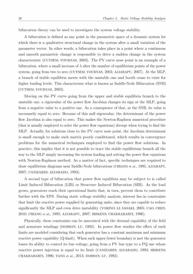
A second type of bifurcation that power flow equilibria may be subject to is calledLimit Induced Bifurcation (LIB) or Structure Induced Bifurcation (SIB). As the loadgrows, generators reach their operational limits that, in turn, prevent them to contributefurther with the EPS. During static voltage stability analysis, interest lies in constraintsthat limit the reactive power supplied by generating units, since they are capable to reducesignificantly the MLP and even drive instability (YORINO; LI; SASAKI, 2005; CAO; CHEN,2010; CHIANG et al., 1995; AJJARAPU, 2007; HISKENS; CHAKRABARTI, 1996).

Physically, these constraints can be associated with the thermal capability of the fieldand armature windings (DOBSON; LU, 1992). In power flow studies the effect of suchlimits are modeled considering that each generator has a constant maximum and minimumreactive power capability (Q-limit). When such upper/lower boundary is met the generatorlosses its ability to control its bus voltage, going from a PV bus type to a PQ one whosereactive power injection is equal to its limit (CANIZARES; ALVARADO, 1993; HISKENS;

CHAKRABARTI, 1996; YANG et al., 2013; DOBSON; LU, 1992).


When such bus type modification takes place, the power flow equations also changeand so does the power flow Jacobian. In nature, this represents a structural alteration inthe Jacobian that is perceive as a discontinuity in the PV curve derivative. Such effect canbe observed in Figure 2.4, where the solid curve represents the actual equilibrium diagramwhen a maximum Q-limit is met by a generator. In the same figure, the red curve portraysthe PV curve when the generator is considered a PQ bus while in the blue curve it is aPV bus. In this graphical example, the generator limit reduced the maximum loadabilityof the system from 𝑃𝑚𝑎𝑥2 to 𝑃𝑚𝑎𝑥1.

Q-limit has

been reached

Q-limit has not

been reached

V Qmax is reached

Saddle-Node

Bifurcation

PPmax1 Pmax2P0

(a) Generator Q-limit does not cause instability.

V

Structure

Induced

Bifurcation

PPmax1 Pmax2P0

Qmax is reached

Q-limit has

been reached

Q-limit has not

been reached

(b) Generator Q-limit causes instability.Figure 2.4: Qualitative effect of a generator Q-limit on PV curves is depicted in the solid line.In the blue and red lines the generator is modeled as a PV and PQ bus respectively.

In addition to reducing the MLP, the Q-limits may also cause instability. Mathemati-cally, this happens when the bus type alteration modify the power flow Jacobian in suchway that the real component of one of its eigenvalues becomes positive. This point iscalled limit or structure induced bifurcation (CANIZARES; ALVARADO, 1993; HISKENS;

CHAKRABARTI, 1996; YORINO; LI; SASAKI, 2005; DOBSON; LU, 1992). Such bifurcation canbe seen in Figure 2.4(b) and compared with the SNB that is indicated in Figure 2.4(a),where the Q-limit does not cause instability but diminishes the MLP.

To obtain PV curves and identify the type and location of bifurcations, it is necessaryto solve the power flow equations as the loading parameter 𝜆 increases. The estimatedMLP depends on how this scalar is related with the actual power system loading, which isthe active and reactive load in each bus. The relationship between 𝜆 and the real powerconsumed in the EPS is determined by the load growth direction �� of (2.2).


2.2 Loading Parameter 𝜆 and the Load Growth Di-rection

Continuation methods are design to calculate the solutions of a set of non-linearequations while one parameter changes continuously. When such techniques are appliedto analyse electric power systems, the parameter that is selected to vary is commonly thesystem loading level, indicated by the Greek letter 𝜆.

This section describes the relationship between the scalar 𝜆 and the active and reactiveloads in each bus of the power system. In this description and throughout the entiredissertation, all loads are considered to be of constant power. In general this is not true,but it constitutes a very severe situation and results in a pessimistic estimative of theVSM, which is desirable for security purposes (MANSOUR, 2013; LONDERO; AFFONSO;

NUNES, 2009).The load parametrization employed here is based on two premisses:

1. As the load parameter 𝜆 increases so does the active and reactive load in each bus.2. When 𝜆 = 1 both the system loading level and the power generation corresponds to

the base case of the EPS. This point should be interpreted as the current operatingpoint of the system.

As a result of that it is possible to write the load growth parametrization with (2.3)and (2.4).

𝑃𝐿𝑖 = 𝑃𝐿0𝑖 + (𝜆 − 1)𝐾𝑃 𝑖𝑃𝐿0𝑖 (2.3)

𝑄𝐿𝑖 = 𝑄𝐿0𝑖 + (𝜆 − 1)𝐾𝑄𝑖𝑄𝐿0𝑖 (2.4)

where 𝑃𝐿𝑖 and 𝑄𝐿𝑖 are the active and reactive loads in bus 𝑖 respectively, 𝑃𝐿0𝑖 and 𝑄𝐿0𝑖 arethe same parameters, but now associated with the base case of the power system (𝜆 = 1).𝐾𝑃 𝑖 and 𝐾𝑄𝑖 determine at which proportion the load in each bus grows, for example, if ata given bus 𝐾𝑃 𝑖 = 2, than its active load increases twice as much as the load associatedwith 𝐾𝑃 𝑖 = 1. The ratio between 𝐾𝑃 𝑖 and 𝐾𝑄𝑖 at a given bus arbitrate how the powerfactor of this load varies as 𝜆 changes. If 𝐾𝑄𝑖 = 𝐾𝑃 𝑖 then the load increases with constantpower factor.

As the load grows, generators need to be dispatched to meed such consumption increase.This is done with equation (2.5).

𝑃𝐺𝑖 = 𝑃𝐺0𝑖 + 𝐾𝐺𝑖

[𝑛𝑏∑

𝑖=1𝑃𝐿𝑖 −

𝑛𝑏∑𝑖=1

𝑃𝐿0𝑖

](2.5)

here, 𝑃𝐺𝑖 and 𝑃𝐺0𝑖 are, respectively, the active power that is injected by the generatorin bus 𝑖 and how much it supplies in the base case. The parameter 𝐾𝐺𝑖 is responsibleto dispatch generators as the load grows. The bigger its value, more load the associatedgenerator would take on.

2.3. Continuation Power Flow (CPFLOW) 31

To assure that the total load increase is met by the generators, the summation of all𝐾𝐺𝑖 needs to be equal to one. In this formulation, the generator associated with the slackbus is responsible to supply the increase in transmission system losses as the load growswith parameter 𝜆.

𝑛𝑏∑𝑖=1

𝐾𝐺𝑖 = 1 (2.6)

To sum up, equations (2.3), (2.4) and (2.5) determine the load growth that occurs inthe power system as a function of the loading parameter 𝜆. This increase happens in adirection that is specified by parameters 𝐾𝐺𝑖, 𝐾𝑃 𝑖, 𝐾𝑄𝑖, 𝑃𝐿0𝑖 and 𝑄𝐿0𝑖. In the power flowproblem presented in (2.2), these parameters define the load growth direction vector (��).

To give a physical meaning to 𝜆 it is possible to affirm that, as long as the base caseloading (𝑃𝐿0𝑖 and 𝑄𝐿0𝑖) does not change, the parameter 𝜆 is monotonically related withthe total load in the EPS and it is possible to write:

𝑛𝑏∑𝑖=1

𝑃𝐿𝑖 = 𝜆𝑛𝑏∑

𝑖=1𝑃𝐿0𝑖 (2.7)

This means that, if 𝜆 = 1.5, then the total active power consumption in the system is50% higher than the base case loading.

2.3 Continuation Power Flow (CPFLOW)

Due to the fact that the Jacobian matrix of the power flow equations is ill conditionednear the MLP, simply increasing the EPS load until divergence of the numerical methodemployed to solve such equations is not an adequate way to estimate the maximum load-ability of the system (CANIZARES; ALVARADO, 1993). To solve this problem continuationmethods are employed. They correspond to the mathematical techniques that trace solu-tions of a set of non-linear equations when one of its parameters changes. The applicationof such methods to trace PV curves characterizes what is known as Continuation PowerFlow (CPFLOW) (CHIANG et al., 1995).

The CPFLOW is regarded as an efficient and precise method to estimate the MLPand obtain PV curves. It became a standard approach to perform Voltage StabilityAssessment (VSA) under a static framework for a known load growth direction and itis also utilized as a comparison benchmark for other techniques being developed (CAO;

CHEN, 2010; LI; CHIANG, 2008b).In general, continuation techniques are divided into four parts, which are described in

the following subsections. They are:o Parametrization;o Prediction;o Correction;o Step length control.


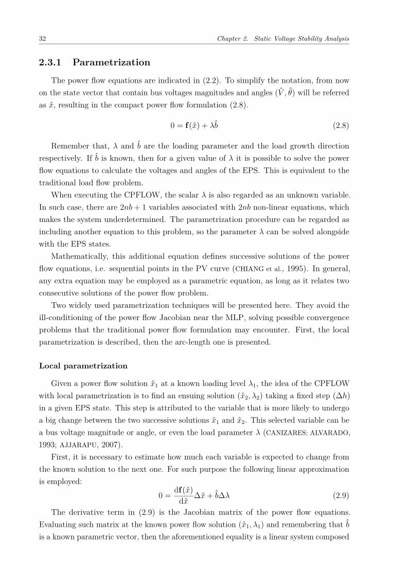
2.3.1 Parametrization

The power flow equations are indicated in (2.2). To simplify the notation, from nowon the state vector that contain bus voltages magnitudes and angles (𝑉 , 𝜃) will be referredas ��, resulting in the compact power flow formulation (2.8).

0 = f(��) + 𝜆�� (2.8)

Remember that, 𝜆 and �� are the loading parameter and the load growth directionrespectively. If �� is known, then for a given value of 𝜆 it is possible to solve the powerflow equations to calculate the voltages and angles of the EPS. This is equivalent to thetraditional load flow problem.

When executing the CPFLOW, the scalar 𝜆 is also regarded as an unknown variable.In such case, there are 2𝑛𝑏 + 1 variables associated with 2𝑛𝑏 non-linear equations, whichmakes the system underdetermined. The parametrization procedure can be regarded asincluding another equation to this problem, so the parameter 𝜆 can be solved alongsidewith the EPS states.

Mathematically, this additional equation defines successive solutions of the powerflow equations, i.e. sequential points in the PV curve (CHIANG et al., 1995). In general,any extra equation may be employed as a parametric equation, as long as it relates twoconsecutive solutions of the power flow problem.

Two widely used parametrization techniques will be presented here. They avoid theill-conditioning of the power flow Jacobian near the MLP, solving possible convergenceproblems that the traditional power flow formulation may encounter. First, the localparametrization is described, then the arc-length one is presented.

Local parametrization

Given a power flow solution ��1 at a known loading level 𝜆1, the idea of the CPFLOWwith local parametrization is to find an ensuing solution (��2, 𝜆2) taking a fixed step (Δℎ)in a given EPS state. This step is attributed to the variable that is more likely to undergoa big change between the two successive solutions ��1 and ��2. This selected variable can bea bus voltage magnitude or angle, or even the load parameter 𝜆 (CANIZARES; ALVARADO,1993; AJJARAPU, 2007).

First, it is necessary to estimate how much each variable is expected to change fromthe known solution to the next one. For such purpose the following linear approximationis employed:

0 = df(��)d��

Δ�� + ��Δ𝜆 (2.9)

The derivative term in (2.9) is the Jacobian matrix of the power flow equations.Evaluating such matrix at the known power flow solution (��1, 𝜆1) and remembering that ��

is a known parametric vector, then the aforementioned equality is a linear system composed


by 2𝑛𝑏 equations and 2𝑛𝑏 + 1 variables (Δ��, Δ𝜆). To solve this system, one arbitrary valueis attributed to either Δ𝜆 or one element of Δ�� (AJJARAPU, 2007). The choice of theparameter that receives the numerical value is also arbitrary, the only criteria that needsto be met is that the resulting linear system, comprised by 2𝑛𝑏 equations, has a singleunique solution. The numerical result of the linear system for (Δ��, Δ𝜆) is numerically thetangent vector of the power system equilibrium diagram at the known power flow solution.This way, employing different parameters with different values to solve this linear system,will result in the same tangent vector direction with distinct magnitudes.

As a result of this process the numerical values of (Δ��, Δ𝜆) are obtained. They are anestimate of how much each state and the loading parameter is expected to change near ��1.The parameter associated with the greatest variation, i.e. the biggest component of thetangent vector, is selected as the local parameter that will be employed in the continuationstep (AJJARAPU, 2007). During the parametrization, the actual numerical values of Δ��

and Δ𝜆 are not of any particular interest, the goal is to select the one that have thegreatest variation to be the continuation parameter. Nevertheless, the calculated tangentvector carry important information regarding the equilibrium point (��1, 𝜆1) and may beused in other stages of the continuation process.

The selected local parameter will be referred with letter 𝑝 and it may be the loadparameter 𝜆, a voltage magnitude or angle . After it is chosen, the goal of the CPFLOWwill be to find a power flow solution (��2, 𝜆2), so that the local parameter meets (2.10).

𝑝2 = 𝑝1 + Δℎ (2.10)

Here, 𝑝1 is the value of the local parameter at the power flow solution (��1, 𝜆1) and𝑝2 will be its value on the next solution to be found (��2, 𝜆2). The step-length Δℎ is aarbitrary parameter that depends on the type of local parameter that is being used, thatis, it can be different if 𝑝 is the loading parameter, a voltage magnitude or angle. Its valueestablishes the separation between two successive power flow solutions that are calculatedwith the continuation method.

It is (2.10) that is included in the set of 2𝑛𝑏 equations of the power flow problem,making equal the number of variables and equations.

Practical use of the locally parametrized CPFLOW demonstrates that, when the powerflow solutions are far from the MLP, the load scalar 𝜆 is the selected local parameter,which is numerically equivalent to solving the traditional power flow problem for a givenvalue of 𝜆. However, if the known solution (��1, 𝜆1) is close to the nose point, bus voltagesare prone to substantial variations, which results in the selection of the most critical busvoltage as the local parameter. This avoids the ill-conditioned Jacobian matrix problemand allows adequate tracing of SNBs (CANIZARES; ALVARADO, 1993).

The graphical interpretation of one continuation step using local parametrization ispresented in Figure 2.5(a), alongside with the arc-length parametrization that will bedescribed in the following topic.


Arc-length parametrization

The goal of the arc-length parametrization is to find the power flow solution (��2, 𝜆2)that is at a distance Δ𝑠 from the already known solution (��1, 𝜆1). This distance is theeuclidean norm in the parametric hyperspace that comprise all EPS states and the loadparameter 𝜆. Mathematically this can be written as:

Δ𝑠2 = ‖��2 − ��1‖22 + (𝜆2 − 𝜆1)2 (2.11)

When this parametrization is employed, (2.11) is added to the set of power flowequations. This way, the load flow problem (2.8) can be simultaneously solved for the busvoltages, angles and 𝜆.

Geometrically, the step Δ𝑠 defines the radius of a hypersphere centered at (��1, 𝜆1). Thenext solution to be calculated is the intersection between such sphere and the equilibriumpoints of the power system (CAO; CHEN, 2010). The equivalent in two dimensions of thisgeometric interpretation is indicated in Figure 2.5(b).

�

p

�h

(x1,�1)^

(x2��2)^

(a) Local parametrization.�

�s

(x1,�1)^

x

(x2��2)^

(b) Arc-length parametrizationFigure 2.5: Graphic interpretation of one continuation step for the two most commonly employedparametrization types.

Just like the local parametrization, the arc-length one avoids the poor conditioning ofthe Jacabian matrix near the maximum loadability point, solving the divergence problemsof the power flow formulation around this point (CHIANG et al., 1995; CAO; CHEN, 2010).

It is worth pointing out that the arc-length parametrization is computationally moreefficient than the local one (CHIANG et al., 1995). It does not require the calculation oftangent vector via the solution of the linear system (2.9), which may be time-consumingfor large power systems.

2.3.2 Prediction

The purpose of the prediction stage is to find an approximate solution (��′2, 𝜆′

2), thatis close to the next power flow solution (��2, 𝜆2) defined by the parametrization equation


and the continuation step employed. This estimate is calculated based on previouslydetermined power flow solutions and curve fitting techniques.

The most commonly employed predictors are based on linear approximations. They arecalled tangent and secant predictors and are described in the following sections (CHIANG

et al., 1995).

Tangent Predictor

As its name portraits, this predictor employs the tangent vector at the last knownpower flow solution to predict the next one. In other words, an approximate power flowsolution is estimated from the PV curve derivative at the last known solution.

In the local parametrization, the tangent vector was calculate to select the localparameter. In the tangent prediction, the same vector is now used to estimate what willbe the states of the power system at the next desired solution. Once again the tangentvector is calculated at the known power flow solution (��1, 𝜆1) with (2.9). This equation isrewritten bellow:

0 = df(��)d��

Δ�� + ��Δ𝜆

As already discussed, to solve this linear system, the power flow Jacobian (derivativeterm) needs to be evaluated in the known equilibrium point (��1, 𝜆1) and one arbitraryvalue needs to be applied to one element of Δ�� or Δ𝜆. When the linear system is solved,the numeric values of Δ�� and Δ𝜆 become known.

With this result and a given continuation step 𝜎, it is possible to estimate the nextpower flow solution with (2.12).

��′2 = ��1 + 𝜎Δ��

𝜆′2 = 𝜆1 + 𝜎Δ𝜆

(2.12)

Overall, the tangent predictor is employed alongside with the local parametrization.Both this steps require the same tangent vector, which means that it is only necessary tosolve the linear system (2.9) once every continuation step and that the predictor itself onlyrequires the operation (2.12) (CANIZARES; ALVARADO, 1993). Nevertheless, this predictorcan be employed with any other parametrization technique, even the arc-length one.

The geometric interpretation of the local predictor is available in Figure 2.6(a).

Secant Predictor

This predictor relies on two previously known power flow solutions to perform a linearcurve fitting and then estimate the next one. If the known solutions are (��0, 𝜆0) and(��1, 𝜆1), this procedure can be done with (2.13) (CHIANG et al., 1995).

��′2 = ��1 + 𝜎(��1 − ��0)

𝜆′2 = 𝜆1 + 𝜎(𝜆1 − 𝜆0)

(2.13)


Predictedsolution

�

x

�

(x1,�1)^

(x'2��'2)^

(a) Tangent predictor.

Predictedsolution

�

x

�

(x1,�1)^(x0,�0)^

(x'2��'2)^

(b) Secant predictor.Figure 2.6: Graphic interpretation of the two most commonly used predictors.

The secant predictor can be compared with the tangent one in Figure 2.6. Thisgeometric interpretation is done in two dimensions to simplify the analysis, nevertheless itis important to remember that the prediction takes place in the complete state space ofthe EPS and also includes the load parameter 𝜆.

Looking at the fact that the secant predictor does not need to solve the linear system(2.9), it is computationally faster when compared to the tangent predictor. Due to thisadvantage, it is commonly employed with the arc-length parametrization, in which case thementioned linear system does not need to be solved (CHIANG et al., 1995). Its disadvantageis that it requires two previous power flow solutions, while the tangent predictor canachieve the same goal with a single one.

2.3.3 Correction

After the prediction stage finds an approximate equilibrium point of the EPS, thecorrection stage is designed to enhance the precision of this operation point by solving thepower flow equations within the desired accuracy tolerance. In other words, its goal is tosolve the non-linear set of equations (2.8) along with the parametric equation to determinebus voltages magnitudes, angles and the loading parameter 𝜆 (CANIZARES; ALVARADO,1993; CHIANG et al., 1995; AJJARAPU, 2007).

In this situation, there are 2𝑛𝑏 + 1 equations and variables that are generally solvedwith the Newton-Raphson method. The starting point of the numeric procedure is theapproximate solution obtained in the prediction stage. Since this result is usually closeto the actual power flow solution, the Newton’s method converges in few iterations(CANIZARES; ALVARADO, 1993; CHIANG et al., 1995; YORINO; LI; SASAKI, 2005).

The predictor employed curve fitting approximations and it is not capable to accountfor possible discontinuities that may be present in power system equilibrium diagrams,as is the case of generators Q-limits. It is the corrector that is responsible to considersuch constraints and other possible discontinuities. This is achieved within the Newton’snumeric procedure with conditions that guarantee that possible limits are not violated.


As a result of that, when any discontinuity is met, the predictor worsen its precision andmore iterations are needed in the correction stage (CHIANG et al., 1995).

The two dimensional graphic interpretation of both the prediction and corrector stagesare available in Figure 2.7. It is worth pointing out, that the solution that is found afterthe corrector depends on the parametrization and the continuation step employed.

x

�

(x1,�1)^

(x2��2)^

(x'2��'2)^

Figure 2.7: Geometric interpretation of the prediction and correction stages of one continuationstep.

2.3.4 Step-Length Control

The continuation step-length Δℎ or Δ𝑠 of the parametrization step and 𝜎 of theprediction one impacts the computational efficiency of the continuation method. Smallsteps lead to good prediction and consequently few corrector iterations, however thenumber of power flow solutions required to trace the PV curve up until the MLP increasessignificantly. If the continuation step-length is too big the opposite happens: less powerflow solutions are calculated, but the number of iterations in each correction stage isincreased (CHIANG et al., 1995).

Overall, employing a small step length is a safe solution to avoid divergence of thecorrector, if the continuation step is too big the prediction may be too far from the actualpower flow solution, which in extreme cases may cause divergence of the corrector. This isespecially true when EPS equilibrium discontinuities are considered.

When dealing with power flow equations and PV curves, the adequate step lengthwould be bigger in the flat portion of the equilibrium diagram, where the load is relativelylow and the states have an approximately linear behavior. Near the MLP this is not trueanymore and small steps should be employed so the nose of the PV curve accurately tracedand convergence problems are avoided. Implementing this logic during the execution ofthe CPFLOW is not a simple task, since the voltage profile of the system is not knownprior to the execution of the continuation method (CHIANG et al., 1995).


A simple way to implement a flexible step-length control is proposed by (AJJARAPU,2007), where the continuation step is calculated depending on how many iterations thecorrector took to converge for the previous solution. This method is indicated in (2.14).

𝜎𝑛𝑒𝑤 = 𝜎𝑜𝑙𝑑𝑁𝑑𝑒𝑠

𝑁𝑖𝑡𝑒

(2.14)

In this equation, the step length 𝜎 increases if the number of corrector iterations 𝑁𝑖𝑡𝑒

is smaller than the desired number 𝑁𝑑𝑒𝑠. The opposite happens when the corrector takesseveral iterations to converge. Ajjarapu (2007) suggests that 6 iterations should be usedas the desired value. However, this choice depends on the power system under analysis.

Other step-length control techniques are available in the literature, this one was selectedmerely to exemplify the logic behind their formulation.

2.3.5 CPFLOW Implementation and Evolution

The complete CPFLOW successively execute the prediction and correction steps, whichresults in several power flow solutions for different values of the loading parameter 𝜆 thatcompose the PV curve. As input, it requires one power flow solution, the load growthdirection and the static models for power system equipment. In most applications the lowerportion of the PV curve is not needed for analysis, in such case the continuation methodcan halt when the MLP is reached. Algorithm 1 depicts the general implementation ofthe CPFLOW.

Algorithm 1 Continuation Power Flow (CPFLOW)Step 1 : Insert EPS data, its current load, and expected growth direction;Step 2 : Solve the traditional power flow problem for the base case load to obtain

the first point of the PV curve;Step 3 : Execute the predictor;Step 4 : Execute the corrector to find another point of the PV curve;Step 5 : Check whether the MLP was reached, if not return to Step 3.

The first time that the prediction stage is performed (Step 3 ), there is only oneknown power flow solution available. This precludes the utilization of the secant predictor,therefore the tangent one needs to be applied.

The CPFLOW is a robust technique capable to trace PV curves solving the numericalproblems related to the ill-conditioned power flow jacobian matrix when the system loadis close to the MLP. In the correction stage the Q-limits of the generators can be included,so their effect are considered in the stability analysis. Overall, this method is widelyapplied to perform static VSA of electric power systems and it has become the standardfor comparison when new techniques are proposed in this area (LI; CHIANG, 2008b; CAO;

CHEN, 2010).Besides its advantages, the CPFLOW usually requires the execution of the Newton–

Raphson method several times before the MLP is reached. For this reason, it may not


comply with computational requirements of real time applications or ones that require thestability assessment of several EPS configurations, as it is the case of contingency analysis(MANSOUR et al., 2013; YORINO; LI; SASAKI, 2005; JIA; JEYASURYA, 2000). For this reason,several studies deal with the computational efficiency of the CPFLOW. Alongside withtime performance, many researchers study the negative effect of Q-limits on the MLP.Interest lie on how to identify such points especially when they cause a bifurcation andhow these discontinuities influence the CPFLOW execution.

That is the case of Cao and Chen (2010), they employed arc-length parametrizationwith the step-length control presented in (2.14) to make the continuation method compu-tationally faster. The authors mentioned that the ideal corrector iterations number shouldbe within two and four. They also proposed the repetition of continuation steps withreduced step-lengths when the system is apparently close to a SIB caused by a Q-limit.With this method it is possible to identify the SIB alongside with the generator thatcaused it, however, for such purpose it requires a few extra continuation steps.

Taylor and Irving (2008) also employed arc-length parametrization. They proposedthat the continuation step Δ𝑠 should be selected in order to predict which is the nextgenerator that will reach its Q-limit. After estimating which is this generator, the proposedmethod employs a few continuation steps to find the power flow solution where this limitis met. This is done repetitively until the MLP. According to the authors, this methodcan estimate the VSM using half of the continuation steps that the traditional CPFLOWwould require.

Yorino, Li and Sasaki (2005) enhanced the work of Hiskens and Chakrabarti (1996).They proposed a parametrization that is based on generators Q-limits. After the predictorand corrector, the method results in the next power flow solution where one generatorreaches its reactive limit. With this method, all Q-limits that happen before the MLPare calculated. The number of continuation steps required is equal to the number of suchconstraints, which can be significantly lower than the standard CPFLOW. The maincontribution of this paper is that the continuation step is automatically selected to beequal to a continuous portion of the PV curve, i.e. the arc between two discontinuities.Due to its contribution regarding non-smooth characteristics of the PV curve, this methodwill be described in details in Section 2.4.

Besides these studies that worked mainly with the performance of the CPFLOW, someresearches dealt with the robustness of such method. Even though it is considered a robusttechnique and has been widely used to assess the VSM of electric power system, in somesituations the CPFLOW may experience convergence difficulties. Since such situations areof particular interest in this dissertation, these problems are described in the followingsection alongside with important contributions made by researchers in this area.


2.3.6 Convergence Problems of the CPFLOW

According to Zhao and Zhang (2006), under certain circumstances the CPFLOW isexpected to fail when tracing EPS equilibrium diagrams. Its corrector may diverge eitherbefore or after the nose of the PV curve, which means that it may compromise an adequateestimate of the VSM.

There are two main types of convergence problems that the continuation power flowmay experience: one caused by inadequate prediction and/or step-length size and anotherdue to the parametrization employed (ZHAO; ZHANG, 2006; NETO; ALVES, 2010).

The first problem is a direct outcome of an inaccurate prediction. For the correctorto converge the initial guess of bus voltages magnitudes and angles need to be withinthe convergence neighbourhood of the desired power flow solution. In other words, thepredicted solution should not lie too far from the equilibrium point that satisfies theparametric equation, otherwise divergence may happen when trying to find this point withnumerical procedures (SUNDHARARAJAN et al., 2003; XU; WANG; AJJARAPU, 2012).

One situation that may yield poor prediction accuracy is when inadequately bigcontinuation steps are used. By its nature, this problem can be easily solved with aproper step-length selection and control. However, it can be significantly aggravated whenequilibrium discontinuities are considered. Predictors are not capable to account for theeffect of such power system sudden changes, in which situation they may result in poorapproximations that, in extreme cases, may cause divergence of the corrector (XU; WANG;

AJJARAPU, 2012). As a consequence of equilibrium discontinuities, simply reducing thestep-length may not solve divergence problems.

The second problem is related with the parametrization employed. Two importantaspects need to be analysed here: (i) whether the inclusion of the parametric equation inthe power flow problem solves the ill-condining of the power flow jacobian matrix near theMLP and (ii) if there is a power flow solution that satisfies the parametric equation. Boththis situations are directly related to the parametrization process and are independent ofthe step-length used (ZHAO; ZHANG, 2006).

Convergence problems may arise with both local and arc-length parametrization andthere is no consensus whether which one is more robust. Chiang et al. (1995), Li andChiang (2008c) openly defend the arc-length parametrization. They argue that evenwith inaccurate predictors this parametrization can reach convergence, which means thatbigger continuation steps can be taken. Indeed such parametrization is widely employed,examples of its application can be seen in (FLUECK; DONDETI, 2000; LI; CHIANG, 2008a;CAO; CHEN, 2010). On the other side, Ajjarapu (2007), Alves et al. (2000), Canizaresand Alvarado (1993) support the local parametrization, attesting that power systemswith local voltage instability characteristics may experience divergence when arc-lengthparametrization is used.

The local voltage instability mentioned is characterized when only a few buses of the


power system suffer unbounded voltage drop, while others can keep their magnitude. In thissituation, some buses have the traditional PV curve profile (Figure 2.8(a)), while for othersthe lower portion of the PV curve have a similar slope to the upper one (Figure 2.8(b))(ZHAO; ZHANG, 2006).

V

P

Vcrit

Pmax

(a) Bus prone to voltage drop.

V

P

Vcrit

Pmax

(b) Bus capable to withstand voltage drop.Figure 2.8: Voltage profile of different buses in a power system that displays local voltageinstability phenomena.

This inclined acute angle in the voltage profile of some buses can indeed cause con-vergence problems for the arc-length parametrized CPFLOW due to ill-conditioning ofits Jacobian matrix (ZHAO; ZHANG, 2006; NETO; ALVES, 2010). Nevertheless, the localparametrization may also go through divergence in this situation if an inadequate loadparameter is selected. For example, suppose that the selected local parameter is thevoltage magnitude of the bus with a profile similar to that of Figure 2.8(b), then, thecorrector may try to find a power flow solution for a non-existing value of such voltage, i.e.a value smaller than 𝑉𝑐𝑟𝑖𝑡. In this case, there is no power flow solution that satisfies theparametric equation and the continuation method diverges.

For the author of this dissertation, there is not a obvious choice between this twoparametrizations to assure convergence of the CPFLOW.

In fact, Zhao and Zhang (2006) acknowledged the difficulties and advantages of the twotraditional parametrization techniques presented here. These authors ended up proposingthat these parametrizations should be used interchangeably, whenever one fails the othershould be employed. In case of divergence, they go even further, proposing that distinctEPS states should also be tested as the local parameter.

Since the parametrization dictates the convergence of the continuation method, somestudies propose new parametrizing equations to solve possible divergence of the CPFLOW.For instance, Neto and Alves (2010) parametrize the PV curve with the slope of onestraight line in the plane of the load parameter 𝜆 and the sum of bus voltage magnitudes.Alves et al. (2000) use the total active power loss of the EPS as the parameter for thecontinuation process.


To deal with possible convergence problems related with inadequate continuationstep-lengths and poor prediction, Xu, Wang and Ajjarapu (2012) proposed a convergencemonitor for the first iteration of the correction stage, which is used to select an adequatecontinuation step. The authors went further to include in the predictor an estimate towhether there is PV curve discontinuity before the next power flow solution. If that is true,then the step length is significantly reduced to avoid problems caused by poor predictiondue to the non-smoothness of the EPS equilibrium diagram.

Besides the aforementioned work, Yorino, Li and Sasaki (2005) also dealt with discon-tinuities that exists in PV curves, particularly the generators Q-limits. Since this work isthe basis for future discussions it deserves its own section.

2.4 Q-limit Guided CPFLOW Proposed by Yorinoet al. (2005)

Yorino, Li and Sasaki (2005) proposed a predictor/corrector scheme to find the powerflow solutions at which generators reach their reactive limits as the load increases in agiven direction. The method calculates the successive Q-limits that happen in the PVcurve prior to the MLP. First, it is predicted what is the next generator that will reach itsreactive constraint. Then, the power flow solution where such limit is reached is calculatedvia a correction stage. Just like the conventional CPFLOW, this method is based on therepetition of a predictor and a corrector.

The prediction and correction stages proposed will be described in the following sectionsalong with a mathematical procedure designed to identify when a Q-limit causes instability,i.e. when they are responsible for a Structure Induced Bifurcation (SIB).

2.4.1 Prediction

Differently from the conventional CPFLOW, the predictor is designed to estimate whatis the next generator that will find its Q-limit, then at which load level this happens and,finally, the EPS bus voltages and angles at this point. For this purpose a linear predictoris employed based on the tangent vector calculated with the linear system (2.9), that isrewritten bellow:

0 = df(��)d��

Δ�� + ��Δ𝜆

The procedure to solve this system was already described in Section 2.3 and it willnot be repeated here. It is important to remember that it results in the tangent vector(Δ��, Δ𝜆) of the EPS equilibrium diagram at a known power flow solution (��1, 𝜆1).

2.4. Q-limit Guided CPFLOW Proposed by Yorino et al. (2005) 43

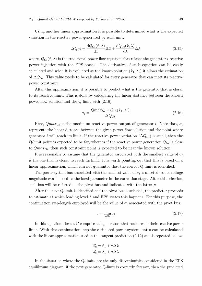
Using another linear approximation it is possible to determined what is the expectedvariation in the reactive power generated by each unit:

Δ𝑄𝐺𝑖 = d𝑄𝐺𝑖(��, 𝜆)d��

Δ�� + d𝑄𝐺𝑖(��, 𝜆)d𝜆

Δ𝜆 (2.15)

where, 𝑄𝐺𝑖(��, 𝜆) is the traditional power flow equation that relates the generator 𝑖 reactivepower injection with the EPS states. The derivative of such equation can be easilycalculated and when it is evaluated at the known solution (��1, 𝜆1) it allows the estimationof Δ𝑄𝐺𝑖. This value needs to be calculated for every generator that can meet its reactivepower constraint.

After this approximation, it is possible to predict what is the generator that is closerto its reactive limit. This is done by calculating the linear distance between the knownpower flow solution and the Q-limit with (2.16).

𝜎𝑖 = 𝑄𝑚𝑎𝑥𝐺𝑖 − 𝑄𝐺𝑖(��1, 𝜆1)Δ𝑄𝐺𝑖

(2.16)

Here, 𝑄𝑚𝑎𝑥𝐺𝑖 is the maximum reactive power output of generator 𝑖. Note that, 𝜎𝑖

represents the linear distance between the given power flow solution and the point wheregenerator 𝑖 will reach its limit. If the reactive power variation (Δ𝑄𝐺𝑖) is small, then theQ-limit point is expected to be far, whereas if the reactive power generation 𝑄𝐺𝑖 is closeto 𝑄𝑚𝑎𝑥𝐺𝑖, then such constraint point is expected to be near the known solution.

It is reasonable to assume that the generator associated with the smallest value of 𝜎𝑖

is the one that is closer to reach its limit. It is worth pointing out that this is based on alinear approximation, which can not guarantee that the correct Q-limit is identified.

The power system bus associated with the smallest value of 𝜎𝑖 is selected, so its voltagemagnitude can be used as the local parameter in the correction stage. After this selection,such bus will be referred as the pivot bus and indicated with the latter 𝑝.

After the next Q-limit is identified and the pivot bus is selected, the predictor proceedsto estimate at which loading level 𝜆 and EPS states this happens. For this purpose, thecontinuation step-length employed will be the value of 𝜎𝑖 associated with the pivot bus.

𝜎 = min𝑖∈𝐺

𝜎𝑖 (2.17)

In this equation, the set 𝐺 comprises all generators that could reach their reactive powerlimit. With this continuation step the estimated power system states can be calculatedwith the linear approximation used in the tangent prediction (2.12) and is repeated bellow:

��′2 = ��1 + 𝜎Δ��

𝜆′2 = 𝜆1 + 𝜎Δ𝜆

In the situation where the Q-limits are the only discontinuities considered in the EPSequilibrium diagram, if the next generator Q-limit is correctly foresaw, then the predicted


power system states are expected to be accurate, since there is no discontinuity between theknown solution and the desired one. This contributes to reduce the number of iterationsrequired by the corrector and may enhance its chance to converge. In this situation, thecontinuation step is automatically selected to be the length of the smooth arc of the EPSequilibrium diagram.

After the pivot bus is selected and the predicted states are calculated, the proceduremoves over to the correction stage.

2.4.2 Correction

The main objective here is to find the power system states where the predicted generatorreaches its Q-limit. The power flow solutions are solved with the Newton-Raphson methodstarting from the predicted voltages and angles (��′

2, 𝜆′2) and resulting in the equilibrium

point where the pivot bus changes from PV to PQ type (��2, 𝜆2).This is possible noticing that at the constraint point, where the generator at bus

𝑝 meets its maximum reactive power supply, the pivot bus satisfies simultaneously theconditions of a PV and a PQ bus. Mathematically this means that:

𝑉 𝑠𝑒𝑡𝑝 − 𝑉𝑝 = 0

𝑄𝑚𝑎𝑥𝐺𝑝 − 𝑄𝐺𝑝 = 0(2.18)

where 𝑉 𝑠𝑒𝑡𝑝 is the specified voltage level for the generator 𝑝 when it is modelled as a PV

bus and 𝑄𝑚𝑎𝑥𝐺𝑝 is its maximum reactive capability.To find the point where these two equations are satisfied, the generator bus is considered

to be of PQ type with reactive power injected equal to 𝑄𝑚𝑎𝑥𝐺𝑝 and the power flow solutionsare simultaneously solved with equation:

𝑉 𝑠𝑒𝑡𝑝 − 𝑉𝑝 = 0 (2.19)

This is the parametric equation of the method proposed by Yorino, Li and Sasaki (2005)and it is conceptually similar to the one utilized in the locally parametrized CPFLOW.However, here, such equation is employed to find the power flow solution where thepredicted generator reaches its Q-limit.

2.4.3 Identification of Structure Induced Bifurcation

Since the method described here finds the discontinuities caused by generators con-straints, Yorino, Li and Sasaki (2005) go on to propose a mathematical algorithm toidentify if a particular Q-limit causes instability, meaning if such point is a SIB.

To achieve such purpose, two conditions that characterize if a power flow solution liein the stable or unstable portion of the PV curve are employed. For that, these conditionsuse the tangent vector (Δ��, Δ𝜆) and Δ𝑄𝐺𝑝.


They are based on the simple consideration that, in the upper and stable portion ofthe PV curve, the inequalities (2.20) need to be satisfied at least for generators that areexpected to reach their Q-limits. After the MLP, the slope of the PV curve is expectedto change for such buses, therefore the two inequalities are not satisfied anymore, whichcharacterizes equilibria in the bellow and unstable part of the PV curve.

Δ𝑉𝑝 ≤ 0Δ𝑄𝐺𝑝 ≥ 0

(2.20)

Those inequalities can be easily justified for stable equilibria. If a generator is going toreach its reactive constraint, then its reactive power is expected to increase as the loadgrows, while its bus voltage is held constant (Δ𝑄𝐺𝑝 > 0 and Δ𝑉𝑝 = 0). If it has alreadymet its limit, then it is not capable to increase its reactive power supply nor to control itsbus voltage, which is expected to fall when 𝜆 increases (Δ𝑉𝑝 < 0 and Δ𝑄𝐺𝑝 = 0).

After the correction stage finds a power flow solution (��2, 𝜆2), two conditions areperformed to identify if this power flow solution is a SIB. The first condition is related towhether the system equilibrium is stable after the Q-limit happened. The second conditionevaluates the equilibrium points prior to the generator constraint.

Condition 1

For this test, the power flow equations employed are the ones when the pivot bus is setto be of PQ type, which represents the power system after the Q-limit. Here, the voltageinequality in (2.20) is tested, since the reactive supply of the unit under analysis is heldconstant. Therefore, the EPS equilibrium points ensuing the Q-limit are stable if Δ𝑉𝑝 < 0.

To calculate this voltage variation, the tangent vector (Δ��, Δ𝜆) to the power flowsolution (��2, 𝜆2) needs to be calculated. This is done solving the linear system in (2.21),remembering that the procedure to do so was already described in Section 2.3.1.

0 = df(��)d��

𝑝 is PQ

(��2,𝜆2)Δ�� + ��Δ𝜆 (2.21)

Δ𝑉𝑝 is one component of the state vector Δ�� that is calculated with the above linearsystem. To asses whether such voltage magnitude is increasing or decreasing all that isnecessary is to observe what is the sign of Δ𝑉𝑝.

Considering that the load is growing (Δ𝜆 > 0) and remembering that such linearapproximation characterizes the power system after the Q-limit happened, then if Δ𝑉𝑝 isnegative the power flow solutions after (��2, 𝜆2) lie in the upper portion of the PV curve,otherwise they are in the bellow one. Two possibilities arise in the latter case: the Q-limitis responsible to cause a bifurcation or the equilibrium point associated with it is unstable.

This means that (2.22) is a necessary but not sufficient condition for the Q-limit to bea SIB. This inequality and the whole procedure described to test it comprise Condition 1


to assess if the power flow solution under analysis is a bifurcation.

Δ𝑉𝑝 > 0 (2.22)

Condition 2

This condition deals with the power system configuration right before the unit meetsits Q-limit. This means that the power flow equations are constructed considering suchgenerator as a PV bus. This time the reactive power inequality in (2.20) is under analysis,since the generator bus voltage is constant.

For this condition, the linear system used to calculate the tangent vector is (2.23).

0 = df(��)d��

𝑝 is PV

(��2,𝜆2)Δ�� + ��Δ𝜆 (2.23)

Even though they are similar, this linear system is slightly different than the one ofCondition 1. One equation of the power flow model changes. In the previous formulation,the pivot bus (𝑝) was considered a PQ bus; now it is a PV one. This yields a differentpower flow jacobian and consequently a distinct tangent vector (Δ��, Δ𝜆).

This time the interest does not lie in a voltage variation, but rather in a reactive powerone. This can be calculated from the tangent vector with equation (2.24), which wasrewritten from (2.15).

Δ𝑄𝐺𝑝 = d𝑄𝐺𝑝

d��

𝑝 is PV

(��2,𝜆2)Δ�� + d𝑄𝐺𝑝

d𝜆

𝑝 is PV

(��2,𝜆2)Δ𝜆 (2.24)

Once again considering that the load is growing before the Q-limit is reached (Δ𝜆 > 0),then the reactive power supplied by this generator is expected to raise (Δ𝑄𝐺𝑝 > 0) if theequilibrium before the power flow solution (��2, 𝜆2) is stable. This situation happens in twopossible scenarios: (i) the point (��2, 𝜆2) itself is a stable equilibrium or (ii) the Q-limitassociated with it causes a SIB. If Δ𝑄𝐺𝑝 < 0, then the critical point has passed and thepower flow solution under analysis is an unstable one.

As a consequence of that, a necessary but not sufficient condition for a SIB is:

Δ𝑄𝐺𝑝 > 0 (2.25)

This inequality together with the procedure to reach it compose Condition 2 to assessif a Q-limit is a SIB.

Summary of Conditions 1 and 2

Condition 1 deals with the power flow solutions that immediately follow the calculatedQ-limit in (��2, 𝜆2), while Condition 2 is associated with the equilibrium points immediatelybefore such solution.


If (2.22) is true, then the power flow solutions after the Q-limit are in the unstableportion of the PV curve. If (2.25) is true, then the equilibria before this constraint isstable. This interpretation is graphically represented in Figure 2.9.

V

�

(x2��2)^

(a) Condition 1 is false (Δ𝑉𝑝 < 0).

V

�

(x2��2)^

(b) Condition 2 is false (Δ𝑄𝐺𝑝 < 0).V

�

(x2��2)^

(c) Condition 1 is true (Δ𝑉𝑝 > 0).

V

�

(x2��2)^

(d) Condition 2 is true (Δ𝑄𝐺𝑝 > 0).Figure 2.9: Graphical interpretation of the conditions proposed to identify if a Q-limit is astructure induced bifurcation.

From this analysis, it is possible to conclude that if Conditions 1 and 2 are simultaneouslysatisfied, then the power flow solution (��2, 𝜆2), where the generator at the pivot bus reachesits Q-limit, is a Structure Induced Bifurcation (SIB).

2.4.4 Implementation and General Aspects of the Method Pro-posed by Yorino et al. (2005)

Just like any continuation method, the general idea of the procedure described here isto repeat the predictor and corrector until the MLP is reached. This method successivelyfinds the PV curve points where generators reach their reactive limits.

Two main drawbacks of this procedure directly follow its main characteristic. First,when the power system is subject to a SNB, it is not capable to trace the voltage profilenear the MLP, since Q-limits may not be available in this region. Second, if the EPS havefew generators prone to meet their Q-limits, then continuation steps become big and the


predictor may be prohibitively inaccurate. In the extreme case where no generators reachtheir constraint, the method is bound to diverge in its the first continuation step.

The second problem is innate to Yorino’s method and when it arises other techniquesneed to be applied. The first problem is solved by the author: the method is designedto execute standard techniques to find the MLP (like the traditional CPFLOW) after anunstable Q-limit equilibrium point, that is not a SIB, is found. This procedure and thegeneral implementation of this method are indicated in Algorithm 2.

Algorithm 2 Procedure to find Q-limits as Proposed by Yorino (2005)Step 1 : Insert EPS data, its current load, and expected growth direction;Step 2 : Solve the traditional power flow problem for the base case load to obtain

the first point of the PV curve;Step 3 : Execute the predictor;Step 4 : Execute the corrector to find a generator Q-limit;Step 5 : Check Condition 1: if false return to Step 3, if true continue to Step 6;Step 6 : Check Condition 2: if false jump to Step 7a, if true jump to Step 7b;Step 7a: Run the traditional CPFLOW to find the SNB between the last two Q-limits;Step 7b: The last Q-limit is identified as a SIB.

This method can be interpreted as a locally parametrized CPFLOW, where the localparameter is selected accordingly to the generators reactive power limits.

In the opinion of the author of this dissertation, the most striking contribution of thismethod is that the continuation step is automatically selected to be the length of onesmooth arc of the PV curve. In other words, if the predictor correctly estimates each oneof the Q-limits, then the power flow solutions found are the discontinuities in the EPSequilibrium diagram. In this situation, every interval between two solutions is necessarilycontinuous and smooth. With this, the predictor is expected to be accurate and thecorrector is unlikely to diverge, which is particularly true if a power system is subject tothe occurrence of several Q-limits not far from each other.

2.5 Final Remarks

The general ideas of the method designed by Yorino, Li and Sasaki (2005) will bethe base of the proposed technique to handle sudden load variations in EPS equilibriumdiagrams. The traditional CPFLOW described here is the standard technique to performVSA in a static framework and will serve for comparison purposes to evaluate the adequacyof the method proposed in this dissertation.

49

Chapter 3Sudden Load Variations on Static

Voltage Stability Analysis

A bulk power system comprises a wide range of devices that influence its steadystate behavior. During PV curve tracing, as the load increases some of these devicesmay suddenly change their parameters according to the EPS states. This is the case ofOLTC transformers, switchable shunt capacitors, excitation limiters of generators andULS protection schemes (XU; WANG; AJJARAPU, 2012). Those examples were not selectedrandomly, they represent discrete changes in the system that, in turn, cause discontinuitiesin its equilibrium diagram. This means that they are responsible to modify the PV curves,so they are not the basic smooth and continuous curves expected.

Of the given examples, switchable capacitors, OLTCs and load shedding schemesare capable to increase bus voltages and may contribute to increase the MLP. However,generator excitation limiters have the opposite effect and may even cause voltage instability.

When using the CPFLOW, such discrete controls are considered during the correctorstage, where conditional tests are employed to verify at every iteration whether or notcontrolled variables reach specified limits (ALVES et al., 2000). For example, whenever agenerator supplies more reactive power than its Q-limit, then the bus type is switchedfrom PV to PQ type.

The prediction stage is based on curve fitting approximations and, therefore, cannottake into account discrete changes on EPS parameters. Therefore, these controls worsenthe accuracy of the predicted solution and increase the number of iterations required bythe corrector of the CPFLOW.

Continuation methods are formally proposed to trace solutions of a set of non-linearsmooth equations while one of its parameter varies continuously. When the aforementionedsudden parametric changes are considered, the power flow equations change whenever alimit is reached. This makes the PV curve non-smooth and discontinuous.

Although this could be a problem, these changes do not present major difficulties tothe traditional CPFLOW. It is common practice to include them during VSA of a power

50 Chapter 3. Sudden Load Variations on Static Voltage Stability Analysis

system. Their main practical consequence is an increase of iterations required by thecorrector to converge.

Nevertheless, this chapter will evidence that when the system undergo severe discretevariations, the discontinuities derived from it can cause convergence problems for theCPFLOW. This may be the case of sudden load variations that power systems may face.Practical examples studied in the following chapters will be the undervoltage mandatorydisconnection of DG units and Undervoltage Load Shedding (ULS).

Besides these two applications, the discussion in this chapter is suitable to evaluate theimpact of any discrete load step in transmission systems caused by undervoltage protectionschemes. It particularly focuses on situations when demand switching is distributedthroughout the network due to local voltage measurements. Hopefully, the numericalresults available in the next two chapters will evidence the usefulness of the discussionprovided here.

In the literature, Zhao and Zhang (2006), Neto and Alves (2010) studied possibleconvergence problems that the traditional CPFLOW may experience. Both of them goon to propose particular parametrization techniques to enhance the convergence rate ofthe continuation method. However, they do not include any discontinuity that may bepresent in the PV curve. Alves et al. (2000), went a little further comparing severalparametrization techniques while accounting for the generator reactive limits and OLTCs,but this work fails to deliver a complete analysis of the effects of these sudden changes onthe convergence of the continuation technique employed.

The work presented by Li and Chiang (2008b) dealt with non-linear characteristic ofloads and its effect on PV curves. Nonetheless, the author refrained from consideringsudden change in EPS demand, which still results in continuous equilibrium diagrams.

Regarding discontinuities caused by contingencies, it is possible to mention the papersof: Flueck and Dondeti (2000), Sundhararajan et al. (2003), Song, Baik and Lee (2006).The last authors developed a convergence monitor to assess whether or not it is possibleto obtain power flow solutions for the incomplete system, starting from the completenetwork solution. Sundhararajan et al. (2003), Flueck and Dondeti (2000) employed acontinuation method that uses a smooth change in the tripped line parameter to track thepost-contingency configuration. Although not originally proposed to asses the effect ofload steps in PV curves, conceptually those papers could be employed to do so. Theirmain inconvenience is that they need to be applied for one known parametric systemdiscontinuity. Therefore, they are not suitable to achieve the objectives of this work, thatconcern successive and distributed load discrete changes throughout the transmissionsystem.

Perhaps the method proposed by Yorino, Li and Sasaki (2005), described in Section 2.4,isthe most appropriate technique to deal with discrete system changes while tracing PVcurves. It finds successive discontinuities in the Jacobian of the power flow equations, i.e.

3.1. PV Curve Discontinuities Produced by Sudden Load Variations 51

in the derivative of EPS equilibria. This is essentially different from sudden load changesthat cause discontinuities in the power system voltages and angles.

Finally, the paper that is closer to the problem under study here, was done byXu, Wang and Ajjarapu (2012). They considered simultaneously switching capacitorsand generator Q-limits, selecting adequate continuation step-lengths to avoid possibleconvergence problems. However, this work did not provide a detailed analysis of the effectof sudden parametric variations in the CPFLOW performance and robustness, particularlyin scenarios where such discontinuities are severe.

In this chapter, a qualitative description of the PV curve discontinuities caused bysudden load variations will be provided in section 3.1. After, a parametrization techniquewill be proposed to deal with such discontinuities in section 3.2. Finally, in section 3.3,the final remarks of this chapter are presented.

3.1 PV Curve Discontinuities Produced by SuddenLoad Variations

Considering three discrete load levels at a particular bus of a transmission system,which will be referred as low, medium and high. As obvious as it may be, it is necessaryto point out that the low level power consumption is smaller than the medium one that, inturn, is lower than the high one. In static analysis, the highest demand levels are expectedto have smaller voltage magnitudes and MLP, effect that is illustrated in Figure 3.1.

V

�

High load

level

�maxhigh �max

med low�max

Medium load

level Low load

level

Figure 3.1: PV curve effect of three different discrete load levels at a particular transmissionsystem bus.

If load switching occurs between these three levels due to an undervoltage protectionscheme, then the power system equilibrium point will experience a jump between PVcurves, which characterizes state discontinuities. This effect is illustrated in Figure 3.2,considering that first the load suddenly increases from the medium level to the high one


and then it reduces to the low one at. Suppose that, at the bus under consideration, this ispossible because a generator is disconnected when its voltage magnitude reaches 𝑉𝑜𝑓𝑓1 andafterwards some load is shed at the voltage 𝑉𝑜𝑓𝑓2. The equilibrium diagram of the EPS isnow given by the solid curve and is inherently discontinuous due to the undervoltage loadswitching.

V

�

High load

level

�maxhigh �max

med low�max

Medium load

levelLow load

levelVoff 1

Voff 2

Figure 3.2: Discontinuities in power systems equilibrium diagrams caused by sudden changesin load. When the bus voltage magnitude reaches 𝑉𝑜𝑓𝑓1 load is switched on, when this value is𝑉𝑜𝑓𝑓2 it is switched off.

Although these discontinuities are essentially load variations for the bulk power system,they do not take place in the abscissa of the equilibrium diagram that represents thesystem loading. That happens because the scalar 𝜆 relates the base case loading to theload of the whole system. In other words, as 𝜆 varies the system demand changes at allbuses accordingly to the growth direction ��, just like it was described in Section 2.2. Aload switching at a single bus does not entail a change in any other part of the system norin the loading parameter 𝜆. Referring to the formulation of Section 2.2, what is modifiedis the base case demand at the bus that experiences the sudden change, that is, 𝑃𝐿0𝑘 and𝑄𝐿0𝑘, where 𝑘 is the referred bus. While the rest of the system does not undergo a loadvariation, the parametric modification at a single bus is responsible to change the powersystem states causing the discontinuities observed.

When the base case load changes, one important aspect of PV curve interpretationis also modified. A EPS with a known base case loading, that is subject to a differentscenario of undervoltage load switching, may end up supplying a different total power forthe same values of 𝜆. This happens because the base case of the system may have beenmodified, which would result in a distinct relation between 𝜆 and the total load connected.During the PV curve scrutiny this means that the same value of 𝜆 may be related to adifferent total load supplied, i.e. that the relationship between 𝜆 and the total active loadis not monotonic.

This can be easily understood considering that a single load is turned on at a particularvalue of 𝜆. Since the system demand in any other bus does not change, then 𝜆 is still


constant. However, the total load connected to the system was increased, due to the loadthat was switched on. This means that the scalar 𝜆 is equal right before and after thedemand is modified, regardless of the fact that for these two points the total active loadconnected to the system changed.

This aspect will be discussed further in the following chapters that present numericalresults.

The impact of load discrete variations on the MLP could be evaluated effortlessly, if theloads that are turned on/off were known beforehand. Unfortunately, when the undervoltageprotections schemes are distributed around the power system, such information is notavailable prior to the PV curve tracing, which will depend on the effect of these protections.This is the case of the two numerical examples given in the following chapters: they arethe mandatory disconnection of distributed generators and disperse undervoltage loadshedding.

As a result of that, these undervoltage protection schemes need to be contemplatedduring the execution of the continuation power flow, like it is already done with generatorreactive power limits, OLTCs and switchable shunt capacitors.

The traditional parametrization techniques employed in the CPFLOW are capable todeal with the discontinuities caused by Q-limits of generators (CHIANG et al., 1995). Suchconstraints cause structural changes in the Jacobian of the power flow equations that, inturn, are responsible for a sudden modification in the derivative of the PV curve. This isin nature different from the load switches that originate discontinuities in EPS states.

Much more similar to sudden load changes are the discontinuities caused by OLTCs andswitchable shunt capacitors. Their effect can also be studied with traditional CPFLOW,just like it was done by Alves et al. (2000), Xu, Wang and Ajjarapu (2012). Althoughstructurally similar to the discontinuities under analysis here, they are expected to bequantitatively different, which is particularly true when big blocs of loads are expected tobe turned on and off.

Before moving on to propose a parametrization technique capable of handling thediscontinuities caused by severe load switching, it is necessary to anticipate whether thetraditional CPFLOW is capable to deal with them.

For the local parametrization, it was seen that the correction step solves the powerflow equations in such a way that the local parameter steps Δℎ from the previously knownequilibrium point.

This parametrization should not entail any convergence difficulty while the continuationparameter is 𝜆, since there is a power flow solution for every value it can assume before theMLP, as can be seen in Figure 3.3 whether the load is stepping up or down. Independentlyof the discontinuity there is always a available power flow solution for the continuationmethod to converge to.

However, near the nose of the PV curve the adequate load parameter is either a bus


V

�

Known

solution

Follow up

solution

�h

(a) Load stepping up.

V

�

Known

solution

Follow up

solution

�h

(b) Load stepping down.Figure 3.3: Qualitative continuation step when the local parametrization is employed while thelocal parameter is the system loading (𝜆).

voltage magnitude or angle. This case is illustrated in Figure 3.4 and its analysis is dividedwhether the load steps up or down.

V

�

Known

solution

Follow up

solution

�h


V

�

Known

solution

Follow up

solution

�h

(b) Load stepping down.Figure 3.4: Qualitative continuation step when the local parametrization is employed while thelocal parameter is a power system state.

The first case can be seen in Figure 3.4(a). Depending on the continuation step (Δℎ)there is a chance that the corrector looks for a solution between the curves where thesystem is with and without the load. In this situation, the solution that satisfies theparametric equation lies in the portion of the PV curve that does not illustrate the actualvoltage profile of the system, i.e. the solid trace. Although this is not ideal, it allows thecontinuation process to proceed towards the MLP. A worse situation could be caused bythe inaccuracy of the predictor, since curve fitting techniques could not possibly predictthe follow up solution. In extreme cases this could lead to divergence of the corrector.

Further observing Figure 3.4(a) it is possible to expect that these problems could besolved by increasing the continuation step. This is not ideal because an adequate step sizeis system dependent and it is generally unknown before executing the CPFLOW. Besidesthat, big steps worsen the predicted solution which can also lead to divergence.

The second case, when the load steps down, is shown in Figure 3.4(b). This time, if the


corrector converges, the power flow solution can only lie in the solid trace that comprisesthe EPS equilibria. Nevertheless, the parametric equation is designed to reduce the busvoltages magnitude, which disguises the actual voltage rise caused by the sudden loadreduction. Furthermore, this discontinuity may also cause divergence of the corrector dueto the predictor accuracy, since it is not capable to anticipate the load switch nor its effecton EPS states.

Converge problems may also happen when the arc-length parametrization is employed,a situation that is illustrated in Figure 3.5, whether the load steps up or down.

V

�

Known

solution

Follow up

solution

�s


V

�

Known

solution

Follow up

solution

�s

(b) Load stepping down.Figure 3.5: Qualitative continuation step when the arc-length parametrization is employed.

This time as well, corrector divergence may follow from poor prediction accuracy causedby the discontinuity.

When the load steps up, depending on the continuation step Δ𝑠, the power flowsolutions that satisfy the parametric equation may not be located in the actual voltageprofile of the system. In this case, the continuation method can proceed to find the MLP,however the PV curve does not depict the equilibrium points of the EPS anymore.

A more critical problem could happen if the continuation step Δ𝑠 is too small. Thissituation is indicated in Figure 3.6, where it is noticeable that there is no power flowsolution that satisfy the arc-length parametric equation. The lack of available solutionwould inevitably entail divergence of the correction stage.

Just like the local parametrization, the convergence problems mentioned here could besolved if the continuation step is big enough. However, the adequate arc-length dependson the problem under analysis and it is unknown a priori.

From this discussion it is possible to conclude that discontinuities caused by suddenload variations disqualify the traditional concept that smaller continuation steps are morerobust than bigger ones. Nevertheless, large steps may not be a viable solution to assureconvergence, after all they worsen the predicted solution accuracy, a circumstance that ismagnified by the fact that the predictor is not capable to account for these discontinuities.

With that in mind, to study the effect of sudden load variations, the CPFLOW requiresan adequate selection of the continuation step to avoid convergence problems. This choice


V

�

Known

solution

�s


V

�

Known

solution�s

(b) Load stepping down.Figure 3.6: Qualitative continuation step when the arc-length parametrization is employed. Thearc-length (Δ𝑠) is so small that there is no power flow solution that satisfies the parametricequation, which causes divergence of the CPFLOW.

is complex and it depends on the power system under analysis and on the size of the loadblocks that are turned on/off.

In extreme situations, there may not be a step length suitable to trace PV curvesconsidering the discontinuities under analysis. This would happen when such discontinuitiesare big enough to require continuation steps so large that the whole continuation process isrendered impossible due to lack of prediction precision. This indicates that the traditionalCPFLOW may be inadequate to study the load sudden changes mentioned here.

The convergence problems foresaw here will be verified in the following chapters thatpresent numerical results.

3.2 Proposed Predictor/Corrector Scheme to HandleSudden Load Variations

The Q-limit guided continuation method proposed by Yorino, Li and Sasaki (2005)is the conceptual basis for the Predictor/Corrector Scheme proposed here to deal withsudden load variations. Perhaps the main insight of the referred paper is to predict thenext discontinuity that will be present in the PV curve and set the continuation stepto find such point. In this case, it is improbable that the continuation process will findconvergence problems due to equilibrium discontinuities, since two successive power flowsolutions will likely be separated by a continuous arc of the curve.

This idea will be employed to handle the sudden load variations that are the subjectof this research. However, it should be emphasised that these discontinuities are in naturedifferent from the ones studied by Yorino, Li and Sasaki (2005). Their main technicalcontributions are adapted to the necessities of the applications desired in this dissertation.

As a result, this section describes a predictor/corrector scheme that aims to successivelyfind the equilibrium points of EPSs right before and right after the occurrence of a load

3.2. Proposed Predictor/Corrector Scheme to Handle Sudden Load Variations 57

switching caused by undervoltage protection schemes. This procedure is divided into fourparts as follows:

o Load Switching Predictiono Correction Stage I - Pre load switchingo Correction Stage II - Post load switchingo Identification of MLP and bifurcation typeEach part will be described separately in the following subsections.

3.2.1 Load Switching Prediction

The goal of this stage is to anticipate what is the next load discontinuity that happensas the load grows and at which power system states it takes place. For that, a linearapproximation based on the tangent vector is employed.

As it was done in Section 2.3.1, the tangent vector of the PV curve at a known powerflow solution (��1, 𝜆) is calculated with equation (2.9), which is rewritten bellow:

0 = df(��)d��

Δ�� + ��Δ𝜆

As already mentioned, to solve this linear system the Jacobian (derivative term) isevaluated at the given equilibrium point and an arbitrary value is attributed to the loadparameter or a state variation (Δ��, Δ𝜆). This value only influences the magnitude of thetangent vector and not its direction. With that, the linear system can be solved for Δ��

and Δ𝜆.Afterwards, for each bus that contains an undervoltage protection capable to switch

loads on or off, the linear distance between the known equilibrium to the point where theprotection trips is estimated with (3.1).

𝜎𝑖 = 𝑉𝑖 − 𝑉 𝑝𝑖𝑐𝑘𝑖

Δ𝑉𝑖

(3.1)

In this equation, 𝑉 𝑝𝑖𝑐𝑘𝑖 is the undervoltage pick-up value that would trigger load

switching in bus 𝑖 and 𝑉𝑖 is the actual bus voltage magnitude at the know power flowsolution ��1. At last, Δ𝑉𝑖 is the component of the tangent vector Δ�� that corresponds tothe bus voltage under analysis. The calculated value 𝜎𝑖 is an estimate of the distance thatbus 𝑖 is from triggering its undervoltage protection. From this interpretation, the nextload discontinuity in the PV curve will be the one associated with the smallest value of 𝜎𝑖.This will be the selected continuation step.

𝜎 = min𝑖∈𝐿

𝜎𝑖 (3.2)

In (3.2) 𝐿 is the set of load buses that employ undervoltage protection schemes. Thebus that is associated with the smallest continuation step (𝜎) will be further used in thecorrection stages indicated by letter 𝑝 and referred as pivot bus.


After the pivot bus and the continuation step-length are determined, EPS states canbe estimated from the tangent vector. These predictions (��′

2, 𝜆′2) serve as the starting

point for the correction stage to find a power flow solution.

��′2 = ��1 + 𝜎Δ��

𝜆′2 = 𝜆1 + 𝜎Δ𝜆

(3.3)

The geometric interpretation of this predictor is indicated in Figure 3.7 whether loadsteps up or down.

V

�

Vppick

(x1,�1)^

(x'2,�'2)^σ


V

�

Vppick

(x1,�1)^

(x'2,�'2)^

σ

(b) Load stepping down.Figure 3.7: Graphical representation of the predictor that estimates what is the next loaddiscontinuity in the PV curve and estimates at which EPS voltages and angles it happens.

Because the predictor relies in a linear approximation and the power flow equations arein nature non-linear, there is no guarantee that the selected pivot bus really correspondsto the next load discontinuity in the PV curve. This means that the power flow solver,i.e. the correction stage, should not ignore the undervoltage protection schemes thatexist in the EPS. At every numeric iteration, the corrector should verify whether anyundervoltage pick-up happens, in which case its effect ought to be considered. This issimilar to what is traditionally done to account for Q-limits in power flow solvers. Theimplication of prediction errors will be addressed again in the description of the correctorsand its practical consequences will be studied in the numerical results.

3.2.2 Correction Stage I - Pre Load Switching

The goal of this stage is to calculate the power flow solutions within the desired accuracyto find the EPS equilibrium point right before the predicted load switching takes place.To achieve that, the power flow problem formulation is augmented with the parametricequation that sets the pivot bus voltage magnitude equal to its undervoltage protectionsetting. That is:

𝑉𝑝 − 𝑉 𝑝𝑖𝑐𝑘𝑝 = 0 (3.4)

The augmented power flow set of equations is solved with the Newton-Raphson method,resulting in the EPS states together with the load parameter (��2, 𝜆2). This is equivalent


to executing a continuation step using local parametrization, where the local parameter isset to be the pivot bus voltage magnitude. Notice that the continuation step-length isautomatically dimensioned to find the discontinuity, as a result of (3.2).

The starting point of the numerical method employed here is the power system statespredicted with (3.3). The outcome of this corrector is indicated in Figure 3.8.

V

�

Vppick

(x1,�1)^

(x'2,�'2)^

(x2,�2)^


V

�

Vppick

(x1,�1)^

(x'2,�'2)^

(x2,�2)^

(b) Load stepping down.Figure 3.8: Graphical representation of Corrector I that solves the power flow equations for theequilibrium point right before the predicted load switching happens.

Since there is no certainty if the pivot bus is the next one to go through a suddenload variation, the corrector should still account for all other undervoltage protectionschemes present throughout the power system. During each iteration of the Newton-Raphson method, bus voltages magnitudes need to be observed to check whether anyother protection is activated. When that happens the respective loads should be turnedon or off accordingly.

3.2.3 Correction Stage II - Post Load Switching

A second corrector is necessary to find the power flow solution right after the loaddiscontinuity takes place. This is different from what was done by Yorino, Li and Sasaki(2005) to find Q-limits that cause a discontinuity in the derivative of the EPS equilibriumstates. These means that these limits are responsible to make the PV curve non-smoothbut continuous, i.e. the equilibrium states immediately before and after the constraint donot change.

Prior to this correction stage, it is not feasible to employ a predictor. This happensbecause it deals with the actual occurrence of the discontinuity, i.e. a jump between twoPV curves. In this situation, approximations based on curve fitting techniques are notexpected to be very accurate, even though their application is not technically impossible.

Sundhararajan et al. (2003) claims that after a sudden variation of power injection,the power flow solution will most likely lie in the vicinities of the equilibrium point thatexisted prior to this change. This justifies not using a predictor and employing the powerflow solution of Corrector I as the seed of the numeric method employed in Corrector II.


With that in mind, the correction stage II will employ the Newton-Raphson methodto find the equilibrium point of the EPS right after the sudden load variation anticipatedby the predictor. The initial guess for this numeric method will be the solution of the firstcorrector.

Just like in the previous corrector, it is important to include in this stage all undervoltageprotection schemes that exist in the power system. This is required to attain possibleundervoltage pick-ups that may take place between the pre and post sudden change inload.

In Corrector II, the parametric equation employed is different whether the load issuddenly increased or reduced, as will be depicted in the following subsections.

Sudden load reduction

It was mentioned in Section 3.1 that right after a sudden load variation, the parameter𝜆 does not change and that the discontinuity is observed in the system voltages and angles.This fact can be well depicted if 𝜆 is selected as the local parameter. This means thatthe power flow equations need to be solved simultaneously with the following parametricequation:

𝜆 − 𝜆2 = 0 (3.5)

where 𝜆2 is the load parameter that was obtained from the corrector stage I.After executing the Newton-Raphson method, the EPS equilibrium calculated will be

(��3, 𝜆3). The parametric equation employed guarantees the load parameter before andafter the sudden load variation will be the same, that is 𝜆3 = 𝜆2. This characterizescorrectly the nature of the discontinuity under analysis. The geometric interpretation ofthis corrector stage is illustrated in Figure 3.9.

V

�

Vppick

(x2,�2)^

(x3,��)^

�2

Figure 3.9: Graphical representation of Corrector II that solves the power flow equations for theequilibrium point right after a predicted load reduction happens.

The parametric equation employed is mathematically equivalent to solve the power flowequations at the load level 𝜆2. As a consequence of that, if this given load level is close to


the MLP, then this corrector may experience convergence problems due to ill-conditioningof its Jacobian matrix. Although this is technically possible it is improbable, because thediscontinuity under analysis is a load reduction responsible to increase the power systemMLP and distance it from 𝜆2.

To be fair, the parametrization employed here does not guarantee the convergence ofthe corrector and contributes negatively to the robustness of the method. However, atleast for the practical application in this dissertation (Undervoltage Load Shedding (ULS)),no significant problems were observed in the tested examples. In this situation, the goal ofthe load discontinuities is to increase the VSM. If divergence arises for a given load that isshed, then the effect of such disconnection is inadequate to increase the MLP significantlyand other ULS scheme should be employed.

Sudden load increase

After a discrete load increase, a reduction in the VSM is expected. Therefore, thereasoning that supported the use of 𝜆 as the local parameter is not valid anymore andother parametrization equation needs to be employed.

In the Corrector I, the pivot bus voltage magnitude was used for that purpose and forsimplicity reasons it is employed once more here. This time, the goal is to obtain a EPSequilibrium point after the load switching under analysis takes place.

The parametric equation employed in this stage is (3.6), where 𝑉𝑝(𝜆2) is the voltagemagnitude of the pivot bus at the solution of Corrector I.

𝑉𝑝 − 𝑉𝑝(𝜆2) = 0 (3.6)

To be thorough, the voltage 𝑉𝑝(𝜆2) is an element of the state vector ��2 and, due to theparametric equation employed in Corrector I (3.4), it is equal to 𝑉 𝑝𝑖𝑐𝑘

𝑝 . Geometrically thiscan be seen in Figure 3.10.

V

�

Vppick

(x2,�2)^

(x3,��)^

Figure 3.10: Graphical representation of Corrector II that solves the power flow equations forthe equilibrium point right after a predicted load increase happens.


With this parametrization, a power flow solution is found keeping the pivot bus voltagemagnitude constant after its load is suddenly increased. To attain such equilibrium point,the total load of the system is reduced, i.e. 𝜆 decreases, as can be seen in Figure 3.10. Theresulting power flow solution does not lie in the system equilibrium diagram. Nevertheless,it allows the predictor/corrector procedure to continue and the next load discontinuity tobe found. In fact, this reduction in load may contribute to the robustness of the method,since it can increase the distances between the calculated power flow solution and the MLP.

After a given load is suddenly increased, bus voltages are expected to drop. Thisreduction can cause pick-up of other undervoltage protection schemes and, consequently,more load discrete steps may follow the first one. Using as example the undervoltagemandatory disconnection of distributed generators, after one unity is disconnected fromthe power system, bus voltages may fall leading to the trip of other units.

The reduction of 𝜆, caused by the parametrization proposed here, facilitates theunderstanding of these successive load steps. It essentially isolates each discontinuity,decreasing the system load after each sudden step up in demand. As will be seen in thenumerical results, this contributes to assure that only the predicted load switching happensin a single continuations step, separating this discontinuity from other ones that woulddirectly result from it.

This parametrization does not disregard the possible cascading effect caused by suddenload increases (generation disconnections) due to undervoltage protections, where oneload stepping up triggers another one to do the same. When this happens, the seconddiscontinuity will lie in the portion of the PV curve where the load parameter is smallerthan the one that originated the first sudden load change.

To clear up, Figure 3.11 exhibit such circumstance. Suppose that a load is steppingup (Δ𝐿1) at (��𝑎, 𝜆𝑎). If it did not cause another undervoltage protection pick-up, thenit would make the system move to operating point (��′

𝑎, 𝜆′𝑎). However, suppose that this

voltage level will also trigger another load to step up (Δ𝐿2) making the actual equilibriumof the system to be (��′′

𝑎, 𝜆′′𝑎).

What the proposed parametric procedure does first is to find the power flow solution(��𝑏, 𝜆𝑏) after Δ𝐿1 as a result of Corrector II. At this equilibrium point, bus voltages arenot expected to have deviated significantly from their pre-swithiching value (��𝑎, 𝜆𝑎), whichmeans that it is highly unlikely that any other undervoltage pick-up happened. Afterwords,the predictor goes on to estimate what is the next undervoltage pick-up and Corrector Iis designed to find at which point it occurs. As a result, the power flow solution foundis (��𝑐, 𝜆𝑐). The voltage at this point is higher then the one that would have followed thefirst load switching Δ𝐿1 at (��𝑎′ , 𝜆𝑎′). This means that the second discontinuity Δ𝐿2 willresult directly from the first one Δ𝐿1. In fact, this will be true if the latter solution liessomewhere in the red portion of the PV curve in Figure 3.11.

To be fair, the solution found after this procedure would be (��𝑐, 𝜆𝑐) and not (��′′𝑎, 𝜆′′

𝑎)


Vp

�

(xa,�a)^(xb,�b)

(xc,�c)(x'a,�'a)

(x''a,�''a)

^

^

^

^

�L1�L2

Figure 3.11: Cascading loads stepping up (generation disconnections) due to undervoltageprotection schemes as attained by the proposed predictor/corrector scheme. The red portion ofthe PV curve represents the locus of power flow solutions where discontinuity Δ𝐿2 is caused bythe predecessor variation Δ𝐿1.

which is the system equilibrium state that would follow Δ𝐿1. The solution found maynot represent the system voltage profile, but it allows to predictor/corrector scheme tocontinue and depicts the order of the cascading events.

Notice that this procedure is expected to isolate each discrete change in one singlecontinuation step. This can strengthen the robustness of the method, because it allowsthe continuation steps to gradually find load discontinuities. Meanwhile, the traditionalCPFLOW would have to deal with a big discontinuity caused by cascading sudden loadvariations.

It is necessary to point out that there is no mathematical guarantee that no parametricvariation would take place between the solutions of Correctors I and II and that eachload discontinuity will be found one by one. This reinforces the need to consider in everycorrection stage all undervoltage protection schemes and their respective consequences inthe power system load.

3.2.4 Identifying the MLP and Bifurcation Type

Executing the predictor and both correctors repetitively will compute the successiveload discontinuities that the power system is subject to. However, the operator is generallyinterested in the maximum loadabiltiy point of the transmission network. Unless one ofthe load discontinuities causes instability, the proposed predictor/corrector scheme shouldbe aided with another tool to find the MLP.

The tangent vector to the PV curve can be used to identify whether or not the MLPhas passed, that is, if a given power flow solution lies in the stable upper portion of the PVcurve or in the unstable lower one (CHIANG et al., 1995; CAO; CHEN, 2010; ZHAO; ZHANG,


2006). Considering this, after every correction step, the tangent vector to the calculatedequilibrium is used to assess if an unstable point was found.

Just to remember, the tangent vector is calculated solving the linear system (2.9),which is rewritten bellow, as described in Section 2.3.1.

0 = df(��)d��

Δ�� + ��Δ𝜆

Undervoltage protection schemes will actuate in buses where the voltage is decreasingwhen the load parameter is increasing. As a consequence of that, the tangent vectorcomponent related to the pivot bus voltage magnitude and the load parameter shouldhave opposite signs, as long as the equilibrium point under analysis is in the upper part ofthe PV curve. Therefore if their signs are equal this indicates that the power flow solutionis an unstable equilibrium. This is carried out with following criteria:

sign(Δ𝑉𝑝) = sign(Δ𝜆) (3.7)

where Δ𝜆 and Δ𝑉𝑝 are components of the tangent vector (Δ��, Δ𝜆).This criteria is mathematically equivalent to Condition 1 of the method proposed by

Yorino, Li and Sasaki (2005) that is described in Section 2.4.3. The only difference is that,now, it is applied to the bus that goes through a load switching instead of a Q-limit.

When (3.7) is satisfied, the proposed method should stop solving the power flowequations and an algorithm should be employed to identify the bifurcation type to whichthe system is subject.

This stopping criteria can be overlooked after Corrector II if the load is suddenlyreduced. In this case, one bus demand steps down while the loading parameter 𝜆 is heldconstant. Therefore the EPS equilibrium is not expected to become unstable.

It was seen in Chapter 2 that besides the common Saddle-Node Bifurcation (SNB),the power flow equations are also subject to Structure Induced Bifurcation (SIB) causedby the reactive limit of power systems generators.

When the load suddenly steps up, it can also cause instability. This is particularlytrue when cascading load increases or generator losses take place (KUNDUR et al., 2004).This instability is caused by a parametric discrete change in the EPS, which is similar tothe bifurcation that results from a Q-limit. In this sense, the bifurcation caused by a loadswitching is also referred as SIB. However, the term Limit Induced Bifurcation should notbe used in this situation, since a limit is not actually met.

When the stopping criteria (3.7) is met, two conditional tests are employed to identifyif the MLP is a saddle-node bifurcation or a structure induced one. These conditions aresummed up in Figure 3.12, where ��𝑠𝑢𝑝 and ��𝑏𝑒𝑙 are the last power flow solutions calculatedthat lie in the superior and inferior portion of the PV curve respectively. ��𝑚𝑎𝑗 is the powerflow solution that corresponds the highest value of the loading parameter 𝜆.

Condition I deals with the situation where one load increase or generation disconnectionprompts instability. In this case, the last two power flow solutions found (��𝑠𝑢𝑝 and ��𝑏𝑒𝑙)


Power flow solutions

xsup, xbel and xmaj

True

False

Structure Induced

Bifurcation

TrueSaddle-Node

Bifurcation

False

^ ^ ^

xsup≠xmaj and xbel≠xmaj^ ^ ^ ^

xbel results from Corrector I

^

Condition I:

Condition II:

Figure 3.12: Conditions to identify whether the power system under analysis is subject to asaddle-node bifurcation or a structure induced one. The latter being caused by a sudden loadvariation.

are not the ones that correspond to the biggest load level (��𝑚𝑎𝑗) due to Corrector B, thatreduces the load parameter 𝜆. This can be understood with Figure 3.13, if the solution��𝑏𝑒𝑙 is an unstable equilibrium point, then the discontinuity that led to this point (Δ𝐿1) isresponsible to cause instability. In other words, if an unstable power flow solution is foundfor a load level smaller than a previous sudden load variation, then the EPS equilibriumright before such discontinuity (��𝑚𝑎𝑗) is a SIB.

Vp

�

(xmaj,�maj)^

(xsup,�sup)

(xbel,�bel)^

^

�L1

SIB

Figure 3.13: Scenario when Condition I is satisfied and one load switching is identified as aStructure Induced Bifurcation (SIB).

Condition II contrasts whether the unstable equilibrium (��𝑏𝑒𝑙) is a result of CorrectorI or II. The first case is in Figure 3.14, where it is possible to see that the bifurcationhappened between two load discontinuities in a continuous arc of the PV curve. As a resultof that, between these two solutions there is necessarily a SNB. This is certainly true if thelast power flow solution found did not flag the existence of another load discontinuity. Inthe situation where this is not true, the system should be further analysed. Nevertheless,


this is highly unlikely and, therefore, it was not treated in the proposed method.

Vp

�

(xmaj,�maj)^

(xsup,�sup)

(xbel,�bel)^

^

=Corrector I

SNB

Figure 3.14: Scenario when Condition II is satisfied and a Saddle-Node Bifurcation (SNB) isidentified.

Whenever the SNB is encountered another method should be employed to accuratelyfind the MLP, since the parametrization described here only searches for discontinuities.For this purpose, the last stable equilibrium is used as the stating point of the traditionalCPFLOW (or any other method that can find SNBs) to estimate the MLP.

The proposed parametrization is expected to assure that the portion of the PV curve tobe traced with the CPFLOW is continuous, since it connects two consecutive discontinuities,therefore convergence problems are not likely to occur.

Still discussing Condition II, consider now that the solution found in the lower portionof the PV curve is a result of Corrector II, just like it is indicated in Figure 3.15. In thiscase, it is clear that the discontinuity under analysis (Δ𝐿1) is responsible for the unstableequilibrium found.

Vp

�

(xmaj,�maj)^

(xsup,�sup)

(xbel,�bel)^

^=

Corrector II

SIB

�L1

Figure 3.15: Scenario when Conditions I and II are not satisfied and one load switching isidentified as a Structure Induced Bifurcation (SIB).


The two conditions proposed here do not require any additional calculation and arecapable of identifying the bifurcation type that the EPS under analysis experiences.Furthermore, in the case where a SIB happens, it is possible to single out which loadsudden variation caused it.

3.2.5 Complete Iterative Predictor/Corrector Scheme to Han-dle Sudden Load Variations

The bifurcation identification process, the stopping criteria, the proposed predictorand both correctors can be bundled together to comprise an iterative method capable ofestimating the effect of sudden load variations on the voltage stability margin of powersystems.

The predictor and both correctors described here are capable to successively find loaddiscontinuities caused by undervoltage protection schemes. After each power flow solutionis calculated, the tangent vector is used to evaluate the stopping criteria. Finally, fromtwo conditions it is possible to identify the bifurcation type that happened. This wholeprocess is schematically described in the flowchart available in Figure 3.16.

Power flow solution and

load growth direction

Load Switching

Prediction

Estimated

MLP

Yes

No

Correction Stage I

Pre Load Switching

Identify bifurcation type

Fig. 3.12

Correction Stage II

Post Load Switching

Test if Eq. (3.7) is true

No

Yes

Test if Eq. (3.7) is true

Figure 3.16: Flowchart of the proposed predictor/corrector scheme capable to identify suddenload variations caused by undervoltage protection schemes and to estimate their impact in themaximum loadability point of power systems.


In principle, this whole process could be seen as a locally parametrized continuationmethod whose step-length is automatically selected to be equal to the next continuousarc of the EPS equilibrium diagram. This means taking large steps in the portion of thecurve where the power system is not subject to parametric discrete changes and smallerones when they take place in close proximity.

The author refrains from referring to the proposed algorithm as a continuation method,despite having its four basic parts: parametrization, prediction, correction and step-length control. This is done for two main reasons: first, the method does not trace theEPS equilibrium diagram (PV curve), which means that voltage profiles do not resultfrom it. Second, there is no rigorous justification to employ continuation methods withdiscontinuous functions and the proposed algorithm is designed to deal with discontinuities.

This method is expected to work well if the EPS is subject to successive load discon-tinuities that are not far from each other. Otherwise, it may derive prohibitively longstep-lengths that could compromise the prediction accuracy and prevent convergence ofthe power flow solver.

It is important to state that the proposed method can be executed together with thetraditional CPFLOW according to specific necessities of power utilities, including in thisstandard VSA tool another capability that may broaden its applicability.

The proposed algorithm can also be simultaneously implemented with the methodproposed by Yorino, Li and Sasaki (2005) that is described in Section 2.4. In this case itis possible to identify whether the next equilibrium discontinuity is a generator Q-limit ora sudden load variation to find the power flow solution where it happens.

3.3 Example of Application for the Proposed Predic-tor/Corrector Scheme

To elucidate any unclear aspects regarding the proposed Predictor/Corrector algorithm,it was employed to obtain two load discontinuities that were introduced in the IEEE 14bus test system. The data regarding this EPS is available in (IEEE, 1993).

In bus 14 two undervoltage protection schemes were included to cause sudden parametricvariations in load. First the load steps up, event caused by a unit disconnection at thereferred bus due to an undervoltage protection pick-up at 0.9 pu. As a result of this trip,the base case load at bus 14 (𝑃𝐿014) goes from 22.35 MW to 29.8 MW. Afterwards, half ofthis load is shed as a consequence of another undervoltage protection set at 0.8 pu, whichresults in a total load at bus 14 of 14.9 MW.

These events amount to three possible configurations for the IEEE 14 bus test system:(i) the complete network, (ii) the network without the disconnected generator and (iii)the network without this unit after load shedding occurs. Each of these configurations

3.3. Example of Application for the Proposed Predictor/Corrector Scheme 69

can be associated with one PV curve for the EPS under analysis, which are presented inFigure 3.17.

Without unit after load shedding

Complete system

Without unit

1.0 1.1 1.2 1.3 1.4 1.5 1.6 1.7 1.8 1.90.5

0.6

0.7

0.8

0.9

1.0

1.1

Load Parameter (λ)

Volt

age

(pu)

Figure 3.17: Bus 14 voltage profile of the IEEE 14 bus test system considering the threeconfigurations that this system is subject to, as a result of sudden variations in load.

As a result of the two load discontinuities considered, the voltage profile of the powersystem becomes the solid curve indicated in Figure 3.18.

Figure 3.18: Bus 14 voltage profile of the IEEE 14 bus test system that results from two suddenload variations.

The power flow solutions calculated with the proposed predictor/corrector schemeare indicted in Figure 3.19 and numbered according to the order that they are attained.Solution number 1 is the known equilibrium point required prior to the execution of theproposed method. Solutions 2 and 4 are calculated with Corrector I and they comprisethe power system equilibrium right before the respective load discrete change happened.


Finally, Solutions 3 and 5 results from Corrector II, when the load steps up and downrespectively.

Figure 3.19: Equilibrium solutions obtained with the proposed method to characterize thesudden variations in load that took place in the IEEE 14 bus test system.

Solution number 3 does not lie in the actual equilibrium diagram of the EPS underquestion, however it allows the predictor/corrector procedure to continue.

Since the MLP is not caused by a load discontinuity, it is not calculated with theproposed method alone. In this situation the method would identify a SNB, therefore theCPFLOW should be employed after the last discontinuity was found.

When implemented alongside with the Q-limit guided continuation power flow pro-posed by Yorino, Li and Sasaki (2005) and described in Section 2.4, the proposed pre-dictor/corrector method can identify whether the next discontinuity is a reactive powerlimit or a load switching and then encounter the equilibrium point where it happens. Forthe IEEE 14 bus test system, this procedure resulted in the sequence of discontinuitiespresented in Table 3.1.

Table 3.1: Sequence of discontinuities calculated with the proposed predictor/corrector methodfor the IEEE 14 bus test system.

Discontinuity Bus SystemLoading (𝜆)

Q-limit 3 1.1970Q-limit 6 1.2186Q-limit 8 1.2669Q-limit 2 1.2670

Load step up 14 1.5133Load step down 14 1.5933

3.4. Final Remarks 71

3.4 Final Remarks

The proposed predictor/corrector scheme is not expected to replace the traditionalCPFLOW or any other standard VSA tool. Its applicability is restricted to analysethe effect of sudden load variations caused by undervoltage protection schemes on thestatic voltage stability of EPSs. This method was designed specifically to deal with thediscontinuities caused by such parametric variations, in which case it is expected to performbetter than the CPFLOW.

In this sense, this procedure can be used as a complementary tool to the CPFLOWenhancing it with new features that could broaden its applicability.

It is also reasonable to expect that the ideas presented here could be useful to dealwith other equilibrium discontinuities that power systems may encounter.

However, it is essential to point out that there is no mathematical guarantee that theproposed method will converge when dealing with sudden load changes. In other words, itis not a definite solution to analyse such discontinuities and further studies could be donein this area.


73

Chapter 4Case Study on Distributed Generation

Mandatory Disconnection

One sudden load variation that is dispersed throughout power system and can negativelyimpact its voltage stability is the mandatory disconnection of Distributed Generation (DG)units (VIAWAN, 2008; WALLING; MILLER, 2002; LONDERO; AFFONSO; NUNES, 2009; YANG

et al., 2013).There is no consensus regarding the definition of DG. However, such paradigm is

usually described as small power generation units connected close to EPS loads (OWENS,2014; WADE, 2006). This dissertation uses the definition that comprises the Brazilianlegislation, where Distributed Generators are electric power units connected directly todistribution systems, as long as they are not hydroelectric plants with installed capacitybigger than 30 MW nor thermal plants with efficiency lower than 75% (PRESIDÊNCIA DA

REPÚBLICA, 2004).Government financial support to expand the use of renewable sources and the electricity

market deregulation created a favourable scenario to increase investments in distributedgeneration (XAVIER DIAS; BOROTNI; HADDAD, 2004). Owens (2014) mentions that out ofthe total word wide installed capacity, the DG penetration increased from 21% in 2000to 39% in 2012. Data collected by WADE (2006) show that more than 30% of the totalinstalled power in several European countries is characterized as DG. In Brazil, it isestimated that this value was equal to 4.4% in 2006 and has grown to about 8% in 2015(SANTOS, 2015).

Distributed generators can reduce distribution and transmission power losses, cancontribute to increase the participation of renewable energy sources in the electricitymarket and can increase the efficiency of the electric generation process (WALLING et

al., 2008; ABRI; MEMBER; ATWA, 2011; BOLLEN; HASSAN, 2011). Even though theseunits are essentially beneficial to EPSs, distribution utilities are concerned with possibleadverse effects that they may have on protection coordination, stability and voltage control(WALLING et al., 2008; YANG et al., 2013; LONDERO; AFFONSO; NUNES, 2009).

74 Chapter 4. Case Study on Distributed Generation Mandatory Disconnection

Distribution networks are generally planned and operated with unidirectional powerflow and passive loads. With the penetration of DG units this paradigm changes andthe network becomes active creating technical difficulties that need to be addressed bydistribution utilities (WALLING et al., 2008).

To mitigate possible adverse effects of DG units, such generators are required to bedisconnected whenever there is a fault or disturbance in the feeder to which they areconnected. This ensures proper performance of the feeder protection and control andprevents islanded operation of DG.

Usually, for such purposes, distribution utilities require under/overvoltage and un-der/overfrequency protection schemes at the DG Point of Common Coupling (PCC)(BLACKBURN; DOMIN, 2006; CHEN; MALBASA; KEZUNOVIC, 2013). The main goal of theseprotections are:

1. If a fault occurs in a feeder with a distributed generator, then this unit needs tobe disconnected to assure that it does not contribute to the fault current nor itcompromises the feeder protection actuation.

2. Dynamic oscillations that DG units may cause in distribution systems need to beisolated, so the unit does not compromise the energy quality at the consumer end.

3. Islanded operation need to be prevented in most situations to assure safe automaticbreaker reclosing and to guarantee complete control of the feeder de-energization bythe utility. This is necessary for the safety of utility employees and consumers.

In some cases, the stipulated protection settings are quite restrictive and inadvertentdisconnections are not uncommon (WALLING; MILLER, 2002; CHEN; MALBASA; KEZUNOVIC,2013). The trip of a distributed generator as a direct consequence of such protectionschemes, or any other utility requirement, is what is refereed in this work as DG mandatorydisconnection.

When assessing the static voltage stability of EPSs, it is expected that DG unitscontribute to increase the system VSM. In static models, DG is portrayed as a negativepower injection and, as such, it lessens the transmission lines loading increasing the systemstability margin (ABRI; MEMBER; ATWA, 2011). However, as the load grows, the systemvoltages tend to decline, even in distribution substation buses. These voltages may reachlevels that could cause pick-up of undervoltage protections located at the DG PCC andconsequently promote the trip of such units. This is equivalent to stepping the load upand may decrease the VSM and even cause instability.

The effect of distributed generators on both transmission and distribution voltagestability was studied by Yang et al. (2013), Londero, Affonso and Nunes (2009), Abri,Member and Atwa (2011), Zhao et al. (2015). However, these authors did not consider theundervoltage protection of DG units, neglecting their potential negative effect in EPSs.

In the studies of Walling and Miller (2002), Chen, Malbasa and Kezunovic (2013), theDG mandatory disconnection was considered during dynamic simulations. Walling and

75

Miller (2002) demonstrated that inadvertent undervoltage trip of a DG unit may causeinstability in bulk power systems. In the work of Chen, Malbasa and Kezunovic (2013), atransmission system MLP was estimated with successive, slow and small increments in itsload. This study concluded that for high DG penetration levels mandatory disconnectionof these units may cause a significant reduction in the VSM.

These studies demonstrated that inadvertent trip of DG units may cause voltagestability problems. However, to the extent of the knowledge of the author, there is nodetailed research in the literature regarding the effect of DG mandatory disconnectionduring static voltage stability analysis. Notably, DG undervoltage disconnections comprisesthe kind of discontinuity that could be studied with the predictor/corrector scheme proposedin the previous chapter.

The undervoltage protection of DG units is the utility requirement that is most likelyto cause stability problems under a static framework. Particular undervoltage settingsdefined by Brazilian distribution utilities are presented in Table 4.1. Notice that the timedelay of such protections are not presented, because they are not relevant during staticanalysis.

Table 4.1: Undervoltage setting at the DG point of common coupling as required by Braziliandistribution utilities.

Distribution Federation Undervoltage ReferenceUtility State Pick-upCOPEL Paraná 0.95 (COPEL, 2014)CELESC Santa Catarina 0.85 (CELESC, 2014)

ELEKTRO São Paulo 0.80 (ELEKTRO, 2013)CEMIG Minas Gerais 0.80 (CEMIG, 2011)

These requirements attest that DG units may be subject to inadvertent disconnectionsand it is reasonable to expect that such events can negatively impact the VSM. This isparticularly true for the very restrictive requirement of COPEL.

The main goal of this chapter is to quantify the effect that DG mandatory disconnectionshave in the VSM of bulk power systems. At the same time, it will demonstrate apractical application of the predictor/corrector algorithm proposed in this dissertation,demonstrating its strengths and drawbacks.

Before actual numerical results are shown, a distribution system model is describedin Section 4.1. This model makes it possible to consider the DG undervoltage protectionschemes during the VSA of transmission systems. The effect of DG disconnections isquantitatively depicted in Section 4.2 for two test systems. These results were obtainedwith the proposed predictor/corrector scheme. The final remarks of this chapter areavailable in Section 4.3.


4.1 Distribution System Model with DG for VoltageStability Assessment of Transmission Systems

In order to predict the mandatory disconnection of distributed generators, it is necessaryto estimate the voltage drop from the substation bus associated with the unit to its PCC.This means that distribution feeder models should be included into the bulk power system.

Simultaneous analysis of transmission and distribution systems is difficult for two mainreasons: (i) these systems have different topological structures, impedance parametersand voltage levels; (ii) they are operated and planned by different companies that usuallyexchange little information (ZHAO et al., 2015). Therefore, including distribution feedermodels into the static analysis of a transmission network is a cumbersome task thatinvolves several uncertainties.

The feeder voltage drop and consequently the DG undervoltage protection actuationdepends on the power injected by such unit, the feeder impedance parameters, its automaticvoltage control and the system loading level. In general, this information is not availableto transmission system utilities, therefore simplifying hypotheses are necessary to accountfor DG mandatory disconnection during the voltage stability assessment of a large EPSs.

Here, three hypotheses are made based on general characteristics of distributionsystems instead of specific data that would probably be unknown to the transmissionsystem operator.

o Hypothesis 1: Substations are equipped with an On-load Tap Changer (OLTC). Thistransformer automatically increases the substation bus voltage in order maintaindistribution feeders in adequate voltage levels. Therefore, it is expected that theOLTC has already achieved its maximum control limit before any DG disconnectiontakes place.

o Hypothesis 2: DG units supply only active power to the distribution system andthis injection is independent of the voltage magnitude at the PCC.

o Hypothesis 3: DG units connected to a given substation can be divided into threegroups according to the voltage drop from the substation to their PCC. The firstgroup is close to the substation and is not subject to voltage drop, the second one islocated at a distance from the substation to which the voltage drop is 0.015 pu and,finally, for the third group this value is equal to 0.030 pu.

Hypothesis 1 is realistic and based on the common practice of employing a transformercapable to change its tap under load in distribution substations. This transformer generallymonitors and controls a downstream bus voltage. From that, it is reasonable to assumethat the control margin of this OLTC has reached its regulation limit before there ispick-up of any DG undervoltage protection. The maximum tap is considered to take placewhen the voltage ratio is 10% above its nominal value (WALLING et al., 2008).

The second hypothesis regards the frequent use of unity power factor control in

4.1. Distribution System Model with DG for Voltage Stability Assessment of Transmission Systems 77

distributed generators (LONDERO; AFFONSO; NUNES, 2009; ABRI; MEMBER; ATWA, 2011;WALLING et al., 2008). In principle, DG units could supply reactive power to the systemassisting the feeder voltage control. Nevertheless, this reactive injection needs to becoordinated with the active voltage control designed by the utility, otherwise the DGunit can conflict with other distribution equipment. To assure safe penetration of DG,there are standards that restrict the implementation of active voltage control in such units(WALLING et al., 2008; ABRI; MEMBER; ATWA, 2011). Beyond that, in Brazil DG investorsare not financially compensated by their reactive support, so they commonly operatesupplying as much active power as possible to maximize their profitability.

The third and last hypothesis requires a higher level of approximation. The alternativeto this approach would depend on information regarding distribution systems that isusually unavailable to transmission operators. In this context, including detailed modelsof distribution feeders would only replace the postulated voltage drops by other unknownparameters and variables of these circuits.

The resulting model from these three hypotheses is indicated in Fig. 4.1.

Bulk Power

SystemOLTC

Substation Bus

Vs

PDG1

PL

Transmission System

Load Bus

Vt

-0,015Vs

PDG2

-0,030Vs

PDG3

Figure 4.1: Proposed distribution system model to account for DG mandatory disconnectionduring static voltage stability assessment of bulk power systems.

This model considers that transmission system load buses are distribution substations.Each substation is associated with three groups of distributed generators, which distinguishdifferent distances that DG units may be from the bulk power system. These three groupsare individually paired with a distinct feeder voltage drop. Considering this and theOLTC, one DG group will have its associated units tipped due to their PCC undervoltageprotection when (4.1) is satisfied.

𝑉𝑡 ≤ 𝑉𝑑𝑟𝑜𝑝 + 𝑉𝑝𝑟𝑜𝑡

1.1 (4.1)

In this inequality, 𝑉𝑡 is the voltage magnitude of an EPS load bus and it correspondsto the high side of a substation OLTC. 𝑉𝑝𝑟𝑜𝑡 is the undervoltage pick-up value of the DGPCC protection. Finally, 𝑉𝑑𝑟𝑜𝑝 is the feeder voltage drop, which can assume the valuesof 0, 0.015 or 0.030 pu depending on the DG group under analysis. The denominator isrelated to the OLTC maximum control margin.

Because of the distribution feeder voltage drop, each DG group undervoltage protectionscheme is expected to disconnect their associated units at different load levels.


To exemplify, if the undervoltage protection is set at 0.95 pu for all units associatedwith a given distribution substation, then the first disconnection will take place at thefarthest group when the respective transmission system bus voltage (𝑉𝑡) reaches 0.894 pu.If the voltage continues to fall, then the mid-distance group will be decoupled from thesystem when 𝑉𝑡 goes under 0.879 pu. Finally, if this voltage magnitude reduces even more,bellow 0.864 pu, then the units near the substation are also disconnected.

4.2 Numerical Results

This section illustrates the application of the proposed predictor/corrector schemedescribed in Chapter 3 and compares it with the traditional locally parametrized CPFLOW.The local parametrization was selected over the arc-length one due to its similarity withthe proposed predictor/corrector algorithm. These two methods were implemented inMATLAB, since commercial software is not designed to account for load discrete variations.

Both the CPFLOW and the proposed predictor/corrector scheme were used to assessthe Voltage Stability Margin (VSM) of two power systems: the IEEE 118 bus test system(IEEE, 1993) and the 107 bus reduced Brazilian interconnected system (ALVES, 2007). TheIEEE system is a well established reference in static analysis, while the Brazilian systemis based on real EPS data and has been thoroughly used by the research group of theauthor. Table 4.2 summarizes a few characteristics of both these systems. Their completedata, including their one-line diagrams, are available in Appendices A and B.

Table 4.2: General characteristics of both the IEEE 118 bus test system and the reducedinterconnected Brazilian system.

IEEE 118 BrazilianNumber of buses 118 107

PV buses 53 23PQ buses 64 83

Number of lines 186 170Load buses 91 39

Total active load (GW) 3.668 12.682

This section will address the effect of the DG mandatory disconnection on the VSM ofboth test systems mentioned. For that, a few simplifying considerations were made, eventhough the two methods employed here are not restricted to them. These assumptions arepresented in the following list:

1. The load growth was parametrized as described in Section 2.2 considering that 𝐾𝑃 𝑖,𝐾𝑄𝑖 and 𝐾𝐺𝑖 are all equal to one for every system bus. This means that, load powerincreases in each bus proportionally to the base case loading with constant powerfactor. Note that all load data are provided in Appendices A and B. Also, to meetthis load increase, generators are dispatched proportionally to their base case active

4.2. Numerical Results 79

power injection. This way the generators that were supplying more power to thesystem in the base case, i.e. the bigger ones, are responsible to take on more load.

2. DG units were included in every load bus according to the model in Figure 4.1. Theauthor recognizes that this is not common. Nevertheless, this assumption is in linewith the principle that every load bus is a possible coupling point for DG. It is worthto emphasize that DG penetration data are not available for both test systems underconsideration, which makes any allocation of such units arbitrary.

3. The percentage of the total load that is supplied by DG units is called DG penetrationlevel. Three levels were considered during the numerical studies: 10%, 20% and30%. For example, the total active power injected by DG in the IEEE 118 bus testsystem is 366.8 MW, when its penetration level is 10%. The lesser penetration levelconsidered (10%) is not far from the DG contribution in Brazil, while the higher one(30%) could be associated with a few European countries.

4. The DG power injection in each load bus was not uniformly distributed throughoutthe transmission system. If this was the case, big bundles of DG units, whosedisconnection could be severe to the system stability, would have been be neglected.The actual power supplied by DG units in each load bus is available in AppendicesA and B.

5. In each load bus, the total DG power injection was equally divided between thethree voltage drop groups of the proposed distribution system model depicted inFigure 4.1.

6. The power supplied by DG units was fully compensated by an equivalent load increase.In other words, after a DG unit is included, the load in its bus is incremented bythe exact the same amount of its injected power. This way the base case does notchange from the bulk power system viewpoint no matter the DG penetration levelconsidered and it represents the power system without mandatory disconnection ofDG units.

7. All distributed generators have the same undervoltage protection setting at theirPCC. The two most stringent undervoltage pick-up values of Table 4.1 were employedseparately to obtain the numerical results of this chapter: that is the COPEL settingof 0.95 pu and the CLELESC one of 0.85 pu.

8. The power flow equations are used to represent power system equilibria.9. The predictor/corrector algorithm described in this dissertation was implemented

together with the method proposed by Yorino, Li and Sasaki (2005). Combinedthey can find the generators reactive power limits as well as the DG disconnectionpoints. Since these two are the only parametric discontinuity types modeled here,the implemented algorithm is expected to successively find all discontinuities thatthe test systems are subject to.

The three DG penetration levels and the two undervoltage protection settings considered


create several scenarios so it is possible to identify situations where the DG mandatorydisconnection is critical to the system stability and situations where it is unimportant.

As mentioned in Chapter 3, the proposed approach to consider discrete load changesdoes not entail a monotonic relationship between the load parameter 𝜆 and the totalload connected to the power system. Although this is generally true, the DG mandatorydisconnection is an exception to that. In this case, referring to the load parametrizationof Section 2.2, the discontinuity is not in 𝑃𝐿0𝑘 or 𝑄𝐿0𝑘 as previously described, but ratherin 𝑃𝐺𝑘. To account for DG, 𝑃𝐷𝐺𝑘 is added to 𝑃𝐺𝑘, representing the DG active powerinjection. Therefore, the load itself is not subject to discontinuities. What does changewhen a DG unit trips is 𝑃𝐷𝐺𝑘 that goes to zero. For the EPS, this looks like a discrete loadincrease, since the amount of power that needs to be delivered through the transmissionsystem suddenly rises.

This means that, rigorously, the DG mandatory disconnection is mathematicallydifferent than the sudden load variations described in the previous chapter. However, innature, DG units turning off can be perceived as such load discontinuities, therefore theproposed predictor/corrector scheme is adequate to study such phenomena.

What results from this discussion is that, when the DG mandatory disconnection isunder analysis, the load parameter 𝜆 represents the total active power of the system, i.e.the relationship between 𝜆 and the active power consumed in the whole EPS is monotonic.

First, the quantitative effect of the DG mandatory disconnection is studied for theIEEE 118 bus test system. Afterwards, the results regarding the 107 bus Brazilian systemare presented.

4.2.1 IEEE 118 bus test system

To define a comparative framework, the numerical results were obtained with theproposed predictor/corrector scheme and the CPFLOW with local parametrization. Thesemethods are considered to have converged, if one unstable equilibrium is found.

The three DG penetration levels and the two undervoltage protection settings consideredcombine to a total of six scenarios.

DG undervoltage protection set at 0.95 pu

For the three cases where the DG undervoltage protection was set equal to 0.95 pu, theMaximum Loadability Point (MLP) and the Voltage Stability Margin (VSM) are indicatedin Tables 4.3 and 4.4, for the CPFLOW and the proposed method respectively. Thesetables also present the absolute amount of DG that was disconnected in MW and thepercentage of the total DG injection that was lost.

With exception of the base case, where the system is not subject to DG mandatorydisconnection, the CPFLOW diverged for every scenario considered, i.e. no solution


Table 4.3: Effect of the DG mandatory disconnection in the IEEE 118 bus test system, when theundervoltage protection setting is 0.95 pu. These results are the outcome of the CPFLOW withlocal parametrization.

DG Penetration𝜆𝑚𝑎𝑥

VSM DG disconnectionlevel (GW) (%) (MW) (%)0% 2.126 4.13 113% – –10% 2.111 4.07 111% 69 19%20% 2.085 3.98 108% 123 17%30% 2.072 3.93 107% 201 18%

Table 4.4: Effect of the DG mandatory disconnection in the IEEE 118 bus test system, whenthe undervoltage protection setting is 0.95 pu. These results are the outcome of the proposedpredictor/corrector scheme.


VSM DG disconnectionlevel (GW) (%) (MW) (%)10% 2.113 4.08 111% 75 21%20% 2.093 4.01 109% 170 23%30% 2.073 3.93 107% 279 25%

was found in the inferior portion of the PV curve. The MLP and VSM indicated inTable 4.3 regard the last power flow solution found before divergence of the method. Thecontinuation step-length employed to find such results culminated from several trial anderror attempts to make the CPFLOW converge and the actual value selected was the oneassociated with the higher loading level of the last converged solution.

The proposed predictor/corrector scheme did converge for these three cases. The VSMof both methods are similar, which indicates that the CPFLOW diverged right before theMLP. Prior to the results obtained with the proposed method, it was not possible to besure whether or not the VSM calculated with the CPFLOW was a precise estimate of theIEEE system stability margin, due to the divergence of the method.

From the result of the proposed scheme, it is possible to affirm that the locallyparametrized CPFLOW was not capable to trace the nose of the PV curve for thebifurcation type that this system is subject to.

Even though the MLP estimated with the CPFLOW turned out to be accurate, thiswas not true for the total amount of DG that was disconnected. This happened becausethe continuation method diverged right before the nose of the PV curve, missing the unitsthat were tripped near the critical point of the IEEE test system. Assuming that thenumerical results obtained from the proposed predictor/corrector procedure are accurate,the error caused by the divergence of the CPFLOW reached 27% regarding the amount ofDG that is disconnected prior to MLP.

The outcome of the proposed predictor/corrector scheme also comprises the sequence ofdiscontinuities to which the power system equilibrium diagram is subject to. Between the


reactive power limits and the DG mandatory disconnections, more than 200 discontinuitiestake place in the IEEE 118 test system prior to the MLP, when the undervoltage settingis equal to 0.95 pu for the three DG penetration levels considered.

First, for ease of analysis, only the last 20 discontinuities of the case where the DGpenetration level is equal to 10% are indicated in Table 4.5.

Table 4.5: Sequence of the last 20 discontinuities of the IEEE 118 bus test system equilibriumdiagram. The undervoltage protection setting of DG units is equal to 0.95 pu and the DGpenetration level is 10%.

Discontinuity Bus Voltage drop System CascadingDG group Loading (𝜆) Events

DG 34 3 2.0971 IsolatedDG 3 3 2.0975

ADG 2 3 2.0968DG 18 3 2.0964DG 1 1 2.0968DG 45 2 2.0980 IsolatedDG 96 2 2.1008 IsolatedDG 84 2 2.1012 IsolatedDG 36 2 2.1040

BDG 35 2 2.1028DG 33 1 2.1035

Q-limit 54 – 2.1054 IsolatedDG 13 2 2.1065 IsolatedDG 117 2 2.1087 IsolatedDG 15 2 2.1113 IsolatedDG 19 1 2.1115

CDG 3 2 2.1108DG 2 2 2.1108

Q-limit 113 – 2.1130 IsolatedQ-limit 10 – 2.1132 Isolated

Notice that two types of discontinuity are considered: the reactive power limit ofgenerators and the DG undervoltage mandatory disconnection. As discussed in Chapter3, the load reduction that is observed in successive DG disconnections is a consequenceof Corrector II that reduces 𝜆 to assure solvabitilty of the power flow equations. Fromthe discussion of Section 3.2.3, if a discontinuity takes place in a load level smaller than aprevious disconnection, then the second parametric change is a direct consequence of thefirst one. With that in mind, all discontinuities can be separated into blocks that groupcascading events. This is indicated in the last column of Table 4.5, where it is possibleto notice isolated events, that do not cause any other discontinuity, and cascading ones,where the first disconnection is responsible for the ones comprised in the same event.


For example, in event A, the trip of DG units located in group 3 of bus 3 is responsibleto reduce power system bus voltages to the extent of causing the disconnection of threeother DG groups located at buses 2, 18 and 1. The same interpretation is valid for thecascading events indicated as B and C.

The traditional CPFLOW does not provide such detailed information regarding equi-libria discontinuities. At most, it can provide which discrete parametric change happenedbetween two calculated power flow solutions. In such case, obtaining the actual sequenceof DG disconnections would require very small continuation steps which could yieldconvergence problems, as described in the previous chapter.

Besides indicating the sequence of discontinuities, the proposed method can also identifythe bifurcation type of the MLP. As a result of the proposed stopping criteria, the lastpower flow solution found (Q-limit of Generator 10) was identified to be unstable. Fromthe test proposed by Yorino, Li and Sasaki (2005) described in Section 2.4.3, this solutionis classified as a SIB, meaning that instability is a direct consequence of Generator 10reaching its reactive limit.

This result helps to explain why the locally parametrized CPFLOW diverged. Sincethe local parameter is selected based on the tangent vector to the PV curve, which cannot foresee discontinuities, its choice may be inadequate near the SIB.

The last discontinuities found in the PV curve of the IEEE test system when the DGpenetration is equal to 20% and 30% are shown in Tables 4.6 and 4.7 respectively. Theseresults can be interpreted like the ones regarding the DG penetration level of 10%.

When the penetration is equal to 20%, the trip of DG group 2 at bus 13 is responsibleto turn off a total of 11 MW of DG, as well as to make two bulk power system generatorsreach their Q-limits. For the case where the penetration is 30%, an even more severeevent happens after the disconnection of DG at bus 3: 78 MW of DG contribution is lostdue their mandatory disconnection and four generators reach their limits. This cascadingevents are so severe that there is no stable equilibrium available to the system operateafterwards.

With these results it is noticeable that as the DG penetration level increases, thedisconnection of such units become more severe to the power system. As a result, theEPS becomes more likely to suffer cascading disconnections and consequently structureinduced instability.

The last solution indicated in the last line of both Tables 4.6 and 4.7 were identified asunstable equilibria. From Condition I of Section 3.2.4, the first discontinuities of the lastevent of each table was identified as a SIB. This means that, when the DG penetration is20%, the disconnection of DG group 1 at bus 36 causes instability. When the penetrationis 30%, the same thing can be asserted about DG group 3 at bus 3.

For these two cases, the CPFLOW diverged right before the occurrence of event A,which represents a severe discontinuity in the EPS equilibrium diagram. This demonstrates


Table 4.6: Sequence of the last discontinuities of the IEEE 118 bus test system equilibriumdiagram. The undervoltage protection setting of DG units is equal to 0.95 pu and the DGpenetration level is 20%.


Q-limit 4 – 2.0844 IsolatedDG 36 2 2.0851

A

DG 35 2 2.0819DG 33 1 2.0848DG 3 3 2.0845DG 2 3 2.0821DG 1 1 2.0826DG 96 2 2.0852 IsolatedDG 84 2 2.0880 IsolatedDG 13 2 2.0919

B

DG 15 2 2.0916DG 19 1 2.0881DG 45 1 2.0870

Q-limit 54 – 2.0869DG 117 2 2.0898

Q-limit 113 – 2.0904DG 34 2 2.0915DG 22 1 2.0914DG 3 2 2.0916DG 2 2 2.0898DG 36 1 2.0930

CDG 35 1 2.0904DG 18 2 2.0907DG 52 3 2.0888

Q-limit 10 – 2.0903

that the traditional continuation method can experience convergence problems due todiscrete load changes and may be inapt to consider such events.

Even though the CPFLOW diverged, it got close enough to the MLP, which makes itpossible to compare its computational efficiency to the proposed method. The latter solvesthe power flow problem twice for every load discontinuity, calculating one equilibrium pointbefore the DG is disconnected and one after. In each penetration levels considered, thisamounted to almost 200 power flow solutions. With the continuation step-length employed,the CPFLOW resulted in a few more equilibrium points. The case that required lesspower flow solutions were the one for which the penetration level was equal to 20%, where219 PV curve points were calculated. This means that the proposed method estimatedthe MLP a little faster than the traditional CPFLOW. Larger continuation step-lengthscould have been employed to reduce the number of power flow solutions required by


Table 4.7: Sequence of the last discontinuities of the IEEE 118 bus test system equilibriumdiagram. The undervoltage protection setting of DG units is equal to 0.95 pu and the DGpenetration level is 30%.

Discontinuity Bus Voltage drop System CascadingDG group Loading (lambda) Events

DG 105 3 2.0636 IsolatedDG 96 2 2.0692 Isolated


A

DG 2 3 2.0686DG 1 1 2.0684DG 19 1 2.0702DG 15 2 2.0672DG 34 2 2.0624DG 22 1 2.0630

Q-limit 113 – 2.0673DG 13 2 2.0677DG 36 1 2.0662DG 35 1 2.0619

Q-limit 54 – 2.0652DG 117 2 2.0664DG 18 2 2.0663DG 3 2 2.0635DG 2 2 2.0600DG 15 1 2.0633DG 34 1 2.0577DG 13 1 2.0588DG 14 3 2.0579DG 117 1 2.0582

Q-limit 73 2.0573DG 52 3 2.0581DG 16 3 2.0582DG 3 1 2.0579DG 2 1 2.0544

Q-limit 10 – 2.0537

the CPFLOW. However, this is not enough to ascertain that this traditional VSA toolis computationally more efficient than the proposed technique. In fact, the CPFLOWcommonly requires many dozens of power flow solutions, which makes the 200 equilibriumpoints calculated by the proposed method a reasonable computational cost to solve theconvergence problems that happened with the continuation power flow.

It is necessary to point out that the predictor/corrector scheme was programmed tonotify and consider the occurrence of any discontinuity that was not anticipated by theproposed predictor. Yet, this did not happen in any of the scenarios studied above. Fromthat, it is possible to conclude that for the IEEE system, two successive discontinuities


are close to each other. Therefore the linear predictor proposed is accurate enough toadequately foresee the next discontinuity that will happen.

To be fair, two disadvantages of the proposed predictor/corrector scheme need tobe mentioned. First, it cannot be used to estimate the power system VSM when theDG mandatory disconnections are not considered. The method only finds parametricdiscontinuities in EPSs, meaning it can not be employed when such discontinuities do notexist. Second, the proposed correctors go back and forward with the loading parameter𝜆, so the method does not result in the system voltage profile, i.e. the PV curve is notestimated.

To observe the DG discontinuities, the PV curve obtained with the CPFLOW beforeit diverged is indicated in Figure 4.2.

1.00.75

0.80

0.85

0.90

0.95

Volt

age

(pu)

1.4 1.8 2.2

Without Mandatory Disc.

10% DG

20% DG

30% DG

Load Parameter (λ)

Figure 4.2: Voltage Profile of bus 118 of the IEEE 118 bus test system considering the DGmandatory disconnection with undervoltage protection set at 0.95 pu for three DG penetrationlevels.

The DG mandatory disconnection does not happen for small load levels, at which busvoltages are close to 1 pu. However, as the load grows, voltages drop and some DG unitsare disconnected due to their undervoltage PCC protection. With that, the voltage profileof the system deflects down from the base case, where mandatory disconnection is notconsidered. It is evident in Figure 4.2 that for higher DG penetration levels, the impact oftheir undervoltage trip is bigger.

Even though the discontinuities caused by DG disconnections are not appreciably big,they are noticeable. This is particularly true for the highest penetration level considered.

Intuitively, it would be expected that high penetration of DG increases the MLP of thesystem, since a big part of the load would be supplied by nearby units. This is true, but isnot observed here because of consideration 6 in page 79. Each DG unit that is includedis followed by an equivalent increase in load. As a result of that, the base case of theEPS does not change with different DG penetration levels. Therefore, the only effect of


such units in the system equilibrium diagram is related to their undervoltage mandatorydisconnection.


Reducing the undervoltage protection setting at the PCC of DG units from 0.95 puto 0.85 pu is expected to significantly diminish the negative effect of their mandatorydisconnection in the EPS. The VSMs estimated employing the lessened undervoltagerequirement are indicated in Tables 4.8 and 4.9 for the CPFLOW and the proposedpredictor/corrector scheme respectively.

Table 4.8: Effect of the DG mandatory disconnection in the IEEE 118 bus test system, when theundervoltage protection setting is 0.85 pu. These results are the outcome of the CPFLOW withlocal parametrization.


VSM DG disconnectionlevel (GW) (%) (MW) (%)0% 2.126 4.13 113% – –10% 2.126 4.13 113% 7.1 1.9%20% 2.126 4.13 113% 14.3 1.9%30% 2.127 4.13 113% 23.8 2.2%

Table 4.9: Effect of the DG mandatory disconnection in the IEEE 118 bus test system, whenthe undervoltage protection setting is 0.85 pu. These results are the outcome of the proposedpredictor/corrector scheme.


VSM DG disconnectionlevel (GW) (%) (MW) (%)10% 2.127 4.13 113% 7.1 1.9%20% 2.127 4.13 113% 14.3 1.9%30% 2.127 4.13 113% 23.8 2.2%

This time the continuation method converged for all cases, i.e. one unstable equilibriumpoint was found. With that, the CPFLOW can be used to validate the results obtainedwith the proposed predictor/corrector procedure. Indeed, they are practically the sameboth for the stability margin and the amount of DG that is disconnected.

The VSM that resulted from the CPFLOW when the DG penetration level is equal to30% was slightly bigger than the other cases considered. The reason why this happenedis merely numerical. Meaning that, the continuation step employed was able to find asolution that is closer to the PV curve nose.

With the reduced undervoltage protection requirement, very few units are disconnected.The impact of DG mandatory disconnections became insignificant for any practical purpose.Since now the DG blocks that are switched off are small, the IEEE power system is not


prone to cascading disconnections. Consequently, the PV curve discontinuities are notsevere enough to yield convergence problems for the continuation method.

For the new protection setting, the proposed method identified that the IEEE testsystem is subject to a SIB caused by Generator 10 reaching its Q-limit, for the three DGpenetration levels considered.

Actually, the Q-limits are essential to the adequate progress of the proposed method.In the three cases, less than six discontinuities resulted from DG disconnections, thereforethe successive calculation of Q-limits is what guarantees the accuracy of the predictorstage and the convergence of the proposed correctors. The predictor was able identifyconsecutive discontinuities and, once again, not even one of them was skipped, situationthat would be flagged in the correction stages. Without the Q-limits, the proposed methodwould most likely have diverged, since the first known power flow solution (𝜆 = 1) is farfrom the first DG trip (𝜆 > 2).

The PV curves obtained when the DG undervoltage protection is equal to 0.85 pu willnot be presented here due to their similarity with the base case voltage profile of Figure4.2. That is the blue curve for the system without mandatory disconnection of DG units.

Partial conclusions

One possible conclusion that can be drawn from all results regarding the IEEE 118 bustest system is that the CPFLOW may be inadequate to assess EPSs voltage stability whenthe same is subject to cascading DG trips which represent large equilibria discontinuities.This is the exact situation where the DG mandatory disconnection significantly impactsthe system. However, when such events are small in size and scarce throughout thebulk power system the opposite is true: the proposed predictor/corrector scheme may gothrough convergence problems while the CPFLOW would yield adequate results.

4.2.2 107 bus reduced interconnected Brazilian test system

The same six scenarios, regarding different DG penetration levels and undervoltageprotection settings, studied with the IEEE test system are repeated for the Brazilian one.


Starting with the 0.95 pu undervoltage protection requirement for DG units. The VSMsof the reduced Brazilian system obtained with the locally parametrized CPFLOW and theproposed predictor/corrector scheme are presented in Table 4.10 and 4.11 respectively.

For the Brazilian system, the CPFLOW diverged for the three DG penetration scenariosconsidered. Once again the MLP obtained with this method is not a reliable estimate ofthe system loadability limit. This is more pronounced for the total amount of DG thatis disconnected, where it is evident that the method diverged before any DG is tripped.


Table 4.10: Effect of the DG mandatory disconnection in the 107 bus reduced interconnectedBrazilian test system, when the undervoltage protection setting is 0.95 pu. These results are theoutcome of the CPFLOW with local parametrization.


VSM DG disconnectionlevel (GW) (%) (GW) (%)0% 1.1149 1.457 11.5% – –10% 1.0891 1.130 8.9% 0 0%20% 1.0891 1.130 8.9% 0 0%30% 1.0891 1.130 8.9% 0 0%

Table 4.11: Effect of the DG mandatory disconnection in the 107 bus reduced interconnectedBrazilian test system, when the undervoltage protection setting is 0.95 pu. These results are theoutcome of the proposed predictor/corrector scheme.


VSM DG disconnectionlevel (GW) (%) (GW) (%)10% 1.0919 1.165 9.2% 0.75 58%20% 1.0892 1.132 8.9% 1.06 42%30% 1.0892 1.132 8.9% 1.10 29%

The three scenarios went through convergence problems at the same point as a result ofconsideration 6 in page 79, which guarantees that the system with different DG penetrationlevels is the same if no unit is disconnected.

With the Brazilian test system as well, several continuation steps-lengths were employedin an attempt to make the continuation power flow converge.

Once again, the proposed method is not adequate to estimate the MLP for the systemwithout mandatory disconnection of DG units, since, in such case, the PV curve lacks thediscontinuities that parametrize the referred method.

The sequence of DG trips and generator Q-limits are presented in Tables 4.12, 4.13and 4.14 when the penetration level is equal to 10%, 20% and 30% respectively. All theseresults consider the DG undervoltage protection set at 0.95 pu.

Differently from the IEEE system, the Brazilian one is much closer to its MLP. As aresult of that, the latter EPS goes through less discontinuities before the PV curve noseis reached. For this reason, all equilibrium discontinuities that happen in the Braziliansystem are indicated in the aforementioned tables.

When the DG penetration level is 10%, there are two cascading disconnections. Forthe first one, called event A, the disconnection of DG group 3 in bus 1015 causes anothertrip in bus 939. For the second event, referred as B, the shutdown of DG group 2 locatedin bus 960 drove the cascading disconnection of eleven DG groups amounting to a loss of571 MW of generation. This is enough to drive instability since the last solution found,the Q-limit of Generator 16, was identified as an unstable equilibrium via the proposedstopping criteria. Since this unstable point follows the trip of a DG group in bus 960, this


Table 4.12: Sequence of discontinuities of the 107 bus reduced Brazilian test system equilibriumdiagram. The undervoltage protection setting of DG units is equal to 0.95 pu and the DGpenetration level is 10%.


DG 960 3 1.0892 IsolatedDG 1015 3 1.0898 ADG 939 3 1.0895DG 834 3 1.0904 IsolatedDG 960 2 1.0919

B

DG 814 3 1.0900DG 1015 2 1.0894DG 939 2 1.0888DG 1504 3 1.0847DG 1504 2 1.0766DG 1504 1 1.0660DG 104 3 1.0575DG 138 3 1.0495DG 104 2 1.0469DG 138 2 1.0382DG 104 1 1.0347DG 138 1 1.0250

Q-limit 16 – 1.0171

incident is classified as a SIB by Condition I of Figure 3.12.



DG 960 3 1.0892

A

DG 1015 3 1.0882DG 939 3 1.0866DG 834 3 1.0841DG 1015 2 1.0846DG 1504 3 1.0807DG 1504 2 1.0571DG 1504 1 1.0229DG 104 3 0.9897DG 104 2 0.9685DG 136 3 0.9447DG 104 1 0.9356

When the DG penetration level is either 20% or 30%, the first DG trip happens at




DG 960 3 1.0892

A

DG 1015 3 1.0862DG 939 3 1.0830DG 1015 2 1.0745DG 1504 3 1.0692DG 1504 2 1.0273DG 1504 1 0.9599DG 104 3 0.8649

bus 960 and it is responsible to cause instability. In other words, the fist power injectiondiscontinuity is severe enough to cause cascading shut-downs and finally prevent the systemto find a stable equilibrium point. This explains why these two scenarios have exactly thesame MLP, that is because the first DG disconnection is a structure induced bifurcation.

In both these cases, the DG disconnections are not progressive and slow as the loadgrows. They comprise a cascading event, where one disconnection is enough to disturbthe EPS to the extent of causing instability. The proposed method satisfactorily depictedthis behavior of the Brazilian system, that was overlooked by the traditional CPFLOW.

There are two main reasons why this happened here and not for the IEEE 118 bus testsystem. First, the Brazilian system operates under a more stressed base case load level,which means that it is closer to its MLP. Second, it has a smaller number of load buses(39 against 91 in the IEEE system). Looking at the fact that the DG power injectionis distributed over such buses, the DG groups for the Brazilian system are considerablybigger. Therefore, the impact of their disconnection is expected to be more severe.

Since the CPFLOW diverged before any DG unit is disconnected, the PV curvesobtained for all penetration levels coincide with the case where no unit is disconnected.Because it is not possible to observe the DG discontinuities, the PV curves of the Braziliansystem will be left out of this text.


Differently from the IEEE system, reducing the PCC undervoltage protection require-ment to 0.85 pu did not solve the divergence problem of the CPFLOW. Once again thecontinuation method had convergence problems right before the fist DG unit is discon-nected, which corroborates the fact that such method may be unsuited to analyse discreteload discontinuities in power system equilibria.

The VSMs estimated with this reduced undervoltage protection requirement are


indicated in Tables4.15 and 4.16 for the two numerical procedures being used in thisresearch.

Table 4.15: Effect of the DG mandatory disconnection in the 107 bus reduced interconnectedBrazilian test system, when the undervoltage protection setting is 0.85 pu. These results are theoutcome of the CPFLOW with local parametrization.


VSM DG disconnectionlevel (GW) (%) (GW) (%)0% 1.1149 1.457 11.5% – –10% 1.1132 1.435 11.3% 0 0%20% 1.1132 1.435 11.3% 0 0%30% 1.1132 1.435 11.3% 0 0%

Table 4.16: Effect of the DG mandatory disconnection in the 107 bus reduced interconnectedBrazilian test system, when the undervoltage protection setting is 0.85 pu. These results are theoutcome of the proposed predictor/corrector scheme.


VSM DG disconnectionlevel (GW) (%) (MW) (%)10% 1.1132 1.436 11.3% 195 15%20% 1.1132 1.436 11.3% 312 12%30% 1.1132 1.436 11.3% 406 11%

Comparing the VSM of the Brazilian system with and without DG mandatory discon-nection, the effect of the 0.85 pu undervoltage setting is practically negligible. This meansthat this softer undervoltage requirement is not expected to cause instability problems.

The Q-limits and DG disconnections identified with the proposed predictor/correctormethod are shown in Tables 4.17, 4.18 and 4.19 for the three DG levels considered.




ADG 1015 3 1.1120DG 939 3 1.1112DG 960 2 1.1087

For the three DG penetration levels studied, an unstable equilibrium resulted fromthe first disconnection, which happens for DG group 3 at bus 960. From Condition I ofSection 3.2.4, this trip is a SIB.





ADG 1015 3 1.1101DG 939 3 1.1080DG 1015 2 1.1011




ADG 1015 3 1.1077DG 939 3 1.1038

The CPFLOW was not capable to find a power flow solution after such discontinuity.The only reason why it accurately calculated the VSM is because it was able to get reallyclose to the EPS equilibrium right before it happened.

Since the first DG unit trip was enough to cause instability for the smallest penetrationlevel studied, any other level bigger than this will have the same stability margin.

For all scenarios considered for the Brazilian system, one DG disconnection wasresponsible to cause instability. This can be easily justified by the fact that such unittrip happened for loading levels close the what would have been the MLP of the systemwithout DG undervoltage disconnections. This means that the system is in the verge ofvoltage collapse before the first unit is tripped, when it actually happens it is enough tocause instability.

Partial conclusions

The numerical results obtained from the 107 bus Brazilian test system corroborate theconvergence problems that the CPFLOW may experience when analysing the equilibriumdiscontinuities caused be the mandatory disconnection of DG units. This time as well,these problems were not experienced by the proposed predictor/corrector scheme.


4.3 Final Remarks

The numerical results regarding DG disconnections evidence the fact that the traditionalCPFLOW may experience convergence problems when the power system is subject to loaddiscontinuities. This was particularly true when big blocks of DG units were turned off,especially when cascading events took place.

The proposed predictor/corrector scheme proved capable to identify these cascadingdisconnections, as well as the events that caused instability and the bifurcation type towhich the power system was subject to.

The numerical results provided here also depict the limitations of the proposed method.No information is obtained regarding the actual voltage profile of the system and itsapplication may be compromised if the EPS does not go under several successive parametricdiscontinuities.

95

Chapter 5Case Study on Dispersed Undervoltage

Load Shedding

Another sudden load variation that is distributed among EPS buses is the Undervolt-age Load Shedding (ULS). The parametric discontinuities caused by such phenomena fitthe description of load switches that can be readily analysed with the proposed predic-tor/corrector scheme.

Load shedding is a last resource but effective method to assure that voltage collapsedoes not happen. It is a corrective measure to restore stability of power systems, if allother possible control actions are unavailable (FENG; AJJARAPU; MARATUKULAM, 1998;AMRAEE et al., 2007; LEFEBVRE; MOORS; CUTSEM, 2003; AFFONSO et al., 2004).

One possible cause of voltage instability is the occurrence of severe contingencies. Afteran EPS goes through a contingency there are two possible outcomes: (i) an adequateoperation point is achieved, but the voltage stability margin is reduced and the systembecomes more vulnerable or (ii) instability will occur and corrective actions need to betaken (AFFONSO et al., 2004).

It is common practice in power systems to plan its expansion and operation, so it iscapable to supply the load even when a single of its components becomes unavailable.This is known as N-1 criteria, which is based on a deterministic assessment of the EPSbehavior after every credible single contingency that the power system may be subject to(KUNDUR et al., 2004). Even though such analysis may comprise several contingencies, it isnot capable of considering all possible scenarios.

The main goal of ULS is to avoid instability after the occurrence of severe contingenciesthat are not included in the deterministic analysis mentioned above. This means that,load shedding is designed for very unlikely scenarios that could be cumbersome to systemoperation and even cause voltage collapse (TAYLOR, 1992; LEFEBVRE; MOORS; CUTSEM,2003; MOORS; LEFEBVRE; CUTSEM, 2001; AFFONSO et al., 2004). In this sense, ULS couldeven be a cost effective measure to prevent the interruption of power supply to criticalloads and expensive manufacturing processes (TAYLOR, 1992; BALANATHAN et al., 1998;

96 Chapter 5. Case Study on Dispersed Undervoltage Load Shedding

AFFONSO et al., 2004). Nevertheless, load shedding is always a last resource and should becarried out if other means like static reactive compensators and switchable shunt capacitorsare unavailable or incapable to restore stability (TAYLOR, 1992; TUAN et al., 1994).

To meet its goals ULS should be carefully designed. Two approaches can be distin-guished with this purpose: the decentralized and the centralized schemes. The centralizedone is based on the status of the complete EPS as measured by the control center. There,the localization and amount of load to be shed is determined via an elaborated set of rulesand the instruction to disrupt load is send through communication networks. The localscheme is simpler and based on local measurements of bus voltages that can automaticallydisconnect their associated loads (AMRAEE et al., 2007). For such purpose, undervoltageprotection schemes are usually employed. As a result of them, load is shed if particularbus voltage magnitudes drop bellow some threshold for a given time (CUTSEM; MOORS;

LEFEBVRE, 2002; TAYLOR, 1992).To adequately select the ULS pick-up value, its time delay and location, dynamic

simulations should be employed, since they accurately depict the system behaviour aftera contingency (LEFEBVRE; MOORS; CUTSEM, 2003; ARNBORG et al., 1997; BALANATHAN

et al., 1998). To maintain an EPS stable, ULS should meet two requirements: (i) theremust be a new stable equilibrium point for the post-contingency configuration and (ii) thesystem dynamic trajectory after the disturbance must be inside the region of attraction ofsuch equilibrium (BALANATHAN et al., 1998).

While the second requirement can only be assessed through time domain simulationsof the non-linear dynamic model of the EPS, the first one can employ static techniques.During the design of ULS, dynamic simulations can be computationally exhaustive, sinceone single undervoltage protection configuration should be capable to avoid instability forseveral scenarios of contingency (LEFEBVRE; MOORS; CUTSEM, 2003).

Therefore, static techniques can and should be used to screen adequate ULS projects toassure the existence of stable equilibrium point after the system goes through a contingency(AFFONSO et al., 2004; TUAN et al., 1994; FENG; AJJARAPU; MARATUKULAM, 1998). Afterthat, dynamic analysis is required to assess whether such equilibrium point is actuallyreached.

The proposed predictor/corrector scheme is capable to analyse the effect of local ULSwithin the framework of static studies. It estimates the VSM of a power system subject toULS when the load grows at given direction. In this case, it also calculates the locationand amount of load that is shed for the undervoltage protection schemes employed.

Due to this nature, it can not depict the load shedding that would occur after acontingency takes place, which makes its application in contingency analysis inadequate.The contribution of the proposed method lies in determining how ULS affects the powersystem when the load increases in a given direction.

One possible practical situation that may benefit from the proposed predictor/corrector

97

scheme is the undervoltage protection of air conditioners in Dubai (DEWA, 2011; KAROUI

et al., 2011). There the Dubai Electricity and Water Authority (DEWA) requires thatevery chiller should be provided with an undervoltage relay with fixed voltage cut-offset at 0.75 pu and whose time delay should be less than 200 ms (DEWA, 2011). Suchrequirement was defined precisely to avoid possible blackouts that may result from voltageinstability. Since a significant part of the load in Dubai is composed of air-conditioners,their undervoltage protection can remarkably help the system during adverse situations.In this scenario, the proposed method could be used to identify which loads would gounder ULS and how this would affect the VSM for a given load growth direction.

Nevertheless, the numerical results presented in this chapter do not comprise theparticular features of the ULS in Dubai. In the following sections, the load blocks thatare shed are much bigger than a single air conditioner and they should be regarded as abundle of several loads that are disconnected simultaneously.

In the literature, there are several studies that proposed different techniques to deter-mine the adequate amount of load to be shed to assure that there is a stable equilibriumafter critical contingencies (TUAN et al., 1994; FENG; AJJARAPU; MARATUKULAM, 1998;AFFONSO et al., 2004; AMRAEE et al., 2007). These studies employ static techniques,however they do not explain what would be the driving force to make the calculatedload shedding possible. In other words, they overlook how the ULS could be practicallyimplemented in power systems and no discussion is presented regarding the application ofundervoltage protection schemes for such purpose.

The same gap can be seen in the works of Arnborg et al. (1997) and Balanathan etal. (1998). Those studies argue that the dynamic behavior of the load governs how muchof it should be shed. Then, this value is calculated base on the parameters of the loaddynamic model. Once again, a practical undervoltage load shedding implementation isnot discussed.

Taylor (1992) directly addresses the design of undervoltage protection schemes for loadshedding purposes. To define design criteria, the author employs time domain simulationsof the EPS after critical disturbances. One important conclusion of such work is thateffective undervoltage cut-off relay setting should be within 0.85 pu and 0.92 pu.

In the same line of work it is possible to mention the papers of Moors, Lefebvre andCutsem (2001), Cutsem, Moors and Lefebvre (2002), Lefebvre, Moors and Cutsem (2003).They designed undervoltage protection schemes to avoid voltage collapse in the Hydro-Québec system. From time domain simulations, five transmission buses were selected toindicate whether the system is going through stability problems. Among other conditions,if the average of the voltage magnitude at these buses is bellow 0.94 pu, then load sheddingstarts according to a priority list.

Beyond the analysis made by Taylor (1992), Lefebvre, Moors and Cutsem (2003), thepredictor/corrector scheme could be employed to assess how the proposed ULS protection


schemes impact the loadability margin of EPS for a given load growth direction. It alsoobtains the buses where load shedding happens, how much of it is disconnected and theorder at which such events take place. All this is done from a static point of view.

It is important to point out that the proposed method is not envisioned to substituteother techniques specifically developed to design ULS. On the contrary, its goal is tocontribute with information regarding the effect of the undervoltage protection schemes asthe load grows.

To exemplify the application of the proposed predictor/corrector scheme in studiesregarding ULS, this chapter will present in Section 5.2 numerical results for the two testsystems employed in the previous chapter (the IEEE 118 bus system and the Brazilianreduced one). They are now implemented with undervoltage load shedding instead of DGunits. The model of decentralized ULS that is employed in such systems is described insection 5.1.

5.1 Decentralized Undervoltage Load Shedding Model

The proposed predictor/corrector scheme was designed to examine load discontinuitiesthat are dispersed throughout the EPS. That is why it is employed here to deal withdecentralized ULS.

To simplify the analysis, the most straightforward undervoltage protection design wasimplemented based on what was described by Amraee et al. (2007), Tuan et al. (1994),Lefebvre, Moors and Cutsem (2003). Three basic rules define such ULS:

1. If the voltage magnitude at a pre-specified bus reaches a threshold, then a fixedamount of its load is disconnected.

2. At pre-specified load buses, the voltage magnitude is monitored even if load sheddinghas already happened. If needed, the undervoltage protection may trigger severalsuccessive load disconnections at the same location.

3. There is a maximum limit of load that can be shed in each bus. This ensures thatcrucial loads remain functioning properly.

Three parameters need to be set for this ULS: the undervoltage cut-off value, the timedelay and the amount of load to be shed (CUTSEM; MOORS; LEFEBVRE, 2002). Just likewith the DG mandatory disconnection, the actual time delay of such protections will notaffect the static analysis performed.

5.2 Numerical Results

This time as well, the results obtained with the proposed predictor/corrector methodwill be compared to the ones from the CPFLOW employing local parametrization. This


parametrization was selected over the arc-length one for the same reason mentioned in theprevious chapter, due to its similarity with the proposed algorithm.

The two EPSs under analysis are also the same, that is the IEEE 118 bus test systemand the reduced Brazilian interconnected system. They were briefly described in thepreceding chapter and their complete characterization is available in Appendices A and B.

The following consideration were made to simplify the analysis regarding ULS. Theyare not necessary to the application of the proposed method nor the CPFLOW. Hypothesis1 and 2 were also employed to study the mandatory disconnection of DG units.

1. The load growth was parametrized as described in Section 2.2 considering that 𝐾𝑃 𝑖,𝐾𝑄𝑖 and 𝐾𝐺𝑖 are all equal to one for every system bus. This means that, load powerincreases in each bus proportionally to the base case loading with constant powerfactor. Note that, all load data are provided in Appendices A and B. Also, to meetsuch load increase, generators are dispatched proportionally to their base case activepower injection. This way the generators that were supplying more power to thesystem in the base case, i.e. the bigger ones, are responsible to take on more load.

2. The power flow equations are used to represent power system equilibria.3. The undervoltage load shedding pick-up level was set equal to 0.9 pu. At pre-specified

load buses, when the voltage magnitude reaches this threshold, 10% of the total loadin the associated bus is disconnected. This setting is in accordance with what wasproposed by Taylor (1992).

4. The active and reactive components of a load are shed in the same proportion, i.e.the load power factor remains constant after ULS.

5. At the buses where ULS is possible, 40% of the load comprises critical consumersthat can not be turned off. That means that 60% of the bus demand may actuallybe shed.

6. The predictor/corrector algorithm described in this dissertation was implementedtogether with the method proposed by Yorino, Li and Sasaki (2005). Combinedthey can find the generators reactive power limits as well as load shedding causeby undervoltage protections. These two are the only parametric discontinuitiesconsidered in the EPSs under analysis.

Its essential to point out the relationship between the loading parameter 𝜆 and theEPS load when the system is subject to ULS.

As mentioned in Section 3.1, the load discontinuities happen in the parameters 𝑃𝐿0𝑘

and 𝑄𝐿0𝑘 that represent the base case loading of the system. This is precisely how ULS ismodeled here. As a result of that, 𝜆 cannot be monotonically related to the total activedemand of the power system anymore. Depending on the amount and location of loadshed, the same value of 𝜆 corresponds to different values of total active load.

Nonetheless, such loading parameter 𝜆 still represents the EPS demand. For thebuses where load shedding does not happen, it still is monotonically related to the power


consumption. Observing that and the fact that the general purpose of ULS is to disconnecta few loads to allow other consumers to be supplied, then the maximum value of 𝜆 shouldstill interest operators.

In such case, the value of 𝜆 at the MLP should not be interpreted as the total activepower in MW that could be supplied by the system, but rather as an indicator of howmuch load can be connected before it goes through voltage collapse.

The numerical results displayed here consider two configurations of the test systems:(i) with the complete network and (ii) without a critical generator. These scenarios wereselected to demonstrate important features of the proposed predictor/corrector algorithm.

5.2.1 IEEE 118 bus test system

For the IEEE system, undervoltage load shedding schemes were implemented in buses2, 3, 7, 11, 13, 14 and 117. These locations where selected based on the sensitivity analysisperformed by Amraee et al. (2007).

Complete network

First, the complete network is analysed and the voltage stability margin of the systemwith and without ULS can be compared in Table 5.1. This table also depicts the absoluteamount of load that is shed and the percentage one relative to the total amount that couldbe shed (129.6 MW). The numerical values regarding load shedding are referred to thedemand of the base case (𝜆 = 1) and should be compared with it.

Table 5.1: Effect of the undervoltage load shedding in the IEEE 118 bus test system withcomplete network.

Method ULS 𝜆𝑚𝑎𝑥VSM Load Shedding

(GW) (%) (MW) (%)

CPFLOW × 2.126 4.13 113% – –X 2.195 4.22 115% 76.2 59%

Proposed X 2.193 4.30 117% 33.3 26%

This study has one essential difference when compared with the one regarding DGmandatory disconnection. This time the load discontinuities are beneficial to the voltagestability and the VSM increases for the system with ULS.

For these results, both the CPFLOW and the proposed predictor/corrector schemeconverged. The value 𝜆𝑚𝑎𝑥 corresponds to the maximum load parameter where the powerflow equations are solved for a stable equilibria. Notice that the biggest value of 𝜆𝑚𝑎𝑥

does not correspond to the maximum VSM anymore. This is a direct consequence of theload shedding itself. For the two methods employed, the system went through different


amounts of shed, which makes their relationship between 𝜆 and the total power supplieddistinct.

The value of 𝜆𝑚𝑎𝑥 indicates how much further the load can increase at every bus thatis not subject to shedding. This is why such loading parameter is still expected to interestpower system operators.

The amount of load that is shed was discrepant for the two methods employed. TheCPFLOW overestimated such value due to the discrete nature of the continuation process.Two successive power flow solutions are separated by a gap that is determined by thecontinuation step-length employed. With this method, it is not possible to isolate theevents between the last stable solution and the first unstable one. In this interval, thereis no certainty whether the load shedding happened before or after the MLP. Sincethe proposed predictor/corrector scheme individually finds the load discontinuities, it isexpected to determine which discontinuities happened prior to the nose of the PV curve,estimating the total ULS more accurately.

The last discontinuities before the MLP calculated with the proposed method arepresented in Table 5.2.

Table 5.2: Sequence of last discontinuities calculated with the proposed predictor/correctormethod for the complete 118 bus IEEE test system with ULS protection schemes.

Discontinuity Bus Load Shedding SystemStage Loading (𝜆)

Q-limit 65 – 1.8574Q-limit 46 – 1.9908

ULS 13 1 1.9967ULS 117 1 2.0293ULS 13 2 2.0438ULS 3 1 2.0627ULS 2 1 2.0910ULS 13 3 2.0979ULS 3 2 2.1128ULS 117 2 2.1235

Q-limit 54 – 2.1253ULS 2 2 2.1483ULS 13 4 2.1586ULS 3 3 2.1710

Q-limit 99 – 2.1778Q-limit 10 – 2.1906Q-limit 4 – 2.1934

The different load shedding stages presented in Table 5.2 are related to the repetitiveactuation of the ULS protection schemes to maintain bus voltage magnitudes above thethreshold value. In each stage, 10% of the load is shed and this may go on until stagenumber six, which represents the limit before only critical loads are connected to the bus


under question.The last solution was identified as a SIB with the conditional test proposed by Yorino,

Li and Sasaki (2005) and described in Section 2.4.3. Since the ULS raises bus voltage mag-nitudes, the cascading scenarios observed when analysing the DG mandatory disconnectionare practically impossible here.

Regarding the computational efficiency, the CPFLOW took 240 continuation stepsbefore reaching the MLP. This number is depends directly on the step-length utilizedand it could have been significantly reduced if a larger value had been employed. Theproposed predictor/corrector scheme estimated the same MLP after calculating 55 powerflow solutions. Therefore, in this particular scenario, the proposed method proved to becomputationally more efficient than the traditional CPFLOW. Overall, this algorithmsolves the power flow equations twice for each sudden load variation that takes placebefore the MLP. This means that, the number of such discontinuities will determine thecomputational effort required by the method.

The author would like to emphasise that the discontinuity predictor was able toaccurately identify the Q-limits and the ULS in the correct order, since the correctorsdid not flag any skipped discontinuity. As already said, this happened because thediscontinuities are successively close to each other and, therefore, the linear predictoremployed is accurate enough to select the next one.

Notice that the proposed method was not used to estimate the MLP of the EPS withoutULS, in which case the equilibrium diagram may lack enough discontinuities for adequateperformance of the algorithm.

Besides that, the predictor/corrector scheme did not obtain the PV curve of the system.Differently from the CPFLOW, that resulted in the voltage profile of bus 14 indicated inFigure 5.1.

In this graphic it is clear that after bus voltages reach small levels, ULS protectionschemes start to act, shedding loading to increase the MLP.

Without a critical generator

The second biggest generator (located at bus 80) was selected to be removed over thefirst one, because the numerical results obtained with this topology demonstrate importantfeatures of the proposed method.

For the IEEE system without this unit, the MLP estimated with the CPFLOW andthe proposed predictor/corrector scheme are indicated in Table 5.3.

To the precision presented, the two methods employed obtained the same VSM forthe IEEE system. They also agreed upon the fact that the MLP is reached before anyload is shed. This fact reduces the number of discontinuities in the EPS equilibria, whichmay interfere with the adequate operation of the proposed method. For the scenarios


Volt

age

(pu)

Load Parameter (λ)

0.90

0.92

0.94

0.96

0.98

1.00

1.0 1.2 1.4 1.6 1.8 2.0 2.2

Without ULS

With ULS

Figure 5.1: Voltage Profile of bus 14 of the IEEE 118 bus test system with and without undervoltage load shedding.

Table 5.3: Effect of the undervoltage load shedding in the IEEE 118 bus test system without thegenerator located at bus 80.


(GW) (%) (MW) (%)

CPFLOW × 1.935 3.43 93% – –X 1.935 3.43 93% 0 0%

Proposed X 1.935 3.43 93% 0 0%

considered, this is the first one where actual discontinuities were skipped, that is to say,the predictor incorrectly selected the next one in the equilibrium loci.

This can be seen in the complete set of discontinuities found with the proposed method,which is indicated in Table 5.4.

In these results it is possible to notice that two Q-limits are skipped. To exemplifynumerically what this means, pay attention to the reactive limit of Generator 56. Afterthe Q-limit of Generator 100 was calculated, the linear predictor employed foresaw thatGenerator 15 would reach its limit next. When the correction stage was trying to find theequilibrium point where this actually happens, it identified that Generator 56 had alsomet its constraint. This means that the reactive limit of Generator 56 lies between theQ-limits of Generators 100 and 15.

It is important to point out that the proposed predictor/corrector scheme consideredthat generator 56 achieved its operational limit right before Generator 15, i.e. thisconstraint is not neglected during the estimate of the MLP. Actually, this Q-limit wasobtained exactly as the CPFLOW does.

Even though skipped discontinuities do not invalidate the results, they may causeconvergence problems for the method. Remember that the main reason why the proposed


Table 5.4: Sequence of discontinuities calculated with the proposed predictor/corrector methodfor the 118 bus IEEE test system without Generator 80 and with ULS protection schemes.


Q-limit 92 – 1.0090Q-limit 76 – 1.0633Q-limit 85 – 1.0956Q-limit 74 – 1.0974Q-limit 100 – 1.1149Q-limit 56 – SkippedQ-limit 15 – 1.2214Q-limit 104 – 1.2309Q-limit 70 – 1.2423Q-limit 1 – 1.2858Q-limit 110 – 1.2969Q-limit 12 – 1.3085Q-limit 18 – 1.3170Q-limit 105 – 1.3178Q-limit 55 – 1.3488Q-limit 36 – 1.3529Q-limit 62 – 1.3965Q-limit 19 – 1.4055Q-limit 34 – 1.4221Q-limit 6 – 1.4820Q-limit 8 – 1.5874Q-limit 99 – 1.6705Q-limit 59 – 1.6891Q-limit 32 – 1.7308Q-limit 49 – 1.7613Q-limit 89 – 1.8885Q-limit 65 – 1.9084Q-limit 10 – 1.9136Q-limit 4 – Skipped

ULS 13 1 1.9346

scheme avoids divergence is because it is designed to take continuation steps with thesame length as a continuous arc of the PV curve. When the predictor skips discontinuities,this is not true anymore and the method is more likely to undergo divergence.

The last power flow solution found with the proposed predictor/corrector methodconcerns undervoltage load shedding. Remember that the last solution calculated is thefirst one in the lower and unstable portion of the PV curve. This means that the solvedULS happens after the MLP.

To identify the bifurcation type, Condition I of Figure 3.12 in Section 3.2.4 was notsatisfied, while Condition II was met. This means that the proposed method classified thecritical point as a SNB. In this case, the CPFLOW is employed to find the MLP starting


from the power flow solution at the Q-limit of Generator 10.This particular case, where there is a skipped discontinuity between the last stable

solution and the first unstable one, lies in the set of scenarios where the proposed methodmay wrongly identify a SNB. This happens because it is not capable assess whether theQ-limit of Generator 4 is a SIB. This possibility was overlooked in the algorithm used toidentify the bifurcation type and it constitutes a gap in the proposed method.

Since the IEEE system without Generator 80 does not go under ULS before the MLP,its PV curve will not be presented here.

5.2.2 107 bus reduced interconnected Brazilian test system

For the Brazilian system, ULS protection schemes were set in buses 138, 140, 536, 1015and 1504. They were selected based on simple trial and error tests, so that load sheddingincreases as much as possible the MLP.

Complete network

First, the VSM of the complete Brazilian network was assessed with the locallyparametrized CPFLOW and the proposed predictor/corrector scheme. The results obtainedare indicated in Table 5.5.

Table 5.5: Effect of the undervoltage load shedding in the 107 bus reduced Brazilian test systemwith complete network.


(GW) (%) (MW) (%)

CPFLOW × 1.1149 1.457 11.5% – –X 1.1389 1.538 12.1% 196 19%

Proposed X 1.1389 1.539 12.1% 196 19%

In this situation the CPFLOW and the proposed method obtained the same results,which helps to validate the technique described in this dissertation. Nevertheless, theCPFLOW was unable to find a solution in the unstable portion of the PV curve, i.e. itdiverged. The proposed technique went further, identifying that the Q-limit of Genera-tor 904 caused a SIB. This indicates that the local parametrization was unable to dealwith this bifurcation and divergence happened right before it. This can be attributedto an inadequate selection of the local parameter near the discontinuity that caused thebifurcation.

While the ULS allowed a noticeable rise in the loading parameter 𝜆𝑚𝑎𝑥, this was not sosignificant for the actual VSM. While the increase in 𝜆𝑚𝑎𝑥 allows the load to grow further,this is achieved through the expense of intentional load shedding, that reduces the total


active demand of the system. Both parameters may interest EPS operators due to theirdifferent interpretation.

The sequence of ULS and Q-limits obtained with the proposed method are presentedin Table 5.6. In this case, two ULS stages were skipped by the linear predictor. It is worthpointing out that, although this is not ideal, it did not cause divergence of the methodnor it greatly compromised its performance.

Table 5.6: Sequence of discontinuities calculated with the proposed predictor/corrector methodfor the complete 107 bus Brazilian reduced test system with ULS protection schemes.


ULS 1015 1 1.0866ULS 1015 2 1.0875ULS 1015 3 1.0884ULS 1015 4 1.0893ULS 1015 5 SkippedULS 1015 6 SkippedULS 140 1 1.1003ULS 1504 1 1.1239ULS 140 2 1.1277

Q-limit 919 – 1.1232Q-limit 904 – 1.1390

The last discontinuity calculated was identified as a SIB with the conditions of Sec-tion 2.4.3 proposed by Yorino, Li and Sasaki (2005). This means that, Generator 904causes instability when it reaches its reactive limit.

Even though the CPFLOW diverged, it did so after all load shedding takes place.Therefore, the PV curves obtained with it depict the effect of the ULS. This can be seenin the voltage profile of bus 976 shown in Figure 5.2.

For small loading levels no load shedding occurs and the PV curves with and withoutULS coincide. As voltage magnitudes reduce, some loads are disconnected which resultingin a increased MLP.

Without a critical generator

Disconnecting the biggest generator of the Brazilian system (Generator at bus 810)and performing the same stability analysis, the results obtained are indicated in Table 5.7.

One more time, the CPFLOW diverged. The results of the proposed predictor/correctorscheme indicate that the convergence problem happened right before the first ULS occurs.This suggests that such divergence is a direct consequence of a load discontinuity.

As a consequence of that, not only when loads are stepping up (DG mandatorydisconnection) that divergence may arise in the CPFLOW. When it suddenly steps down,the same problem may occur.


0.90

0.94

0.98

0.86

0.82

1.02

1.00 1.05 1.10 1.15

Volt

age

(pu)

Load Parameter (λ)

Without ULS

With ULS

Figure 5.2: Voltage Profile of bus 976 of the 107 bus Brazilian reduced test system with andwithout under voltage load shedding.

Table 5.7: Effect of the undervoltage load shedding in the 107 bus reduced Brazilian test systemwithout the generator located at bus 810.


(GW) (%) (MW) (%)

CPFLOW × 1.1088 1.380 10.9% – –X 1.0774 0.981 7.7% 0 0%

Proposed X 1.1812 1.867 14.7% 365 36%

The sequence of discontinuities that the Brazilian system undergo as obtained by theproposed method are indicated in Table 5.8.

Once more the predictor proposed skipped two discontinuities. However, this did notentail any problems to the adequate execution of the method. Remembering that theskipped events are not neglected, they are recognized during the correction stages andincluded in the analysis.

The Q-limit of Generator 904 was identified to lie in the unstable portion of the PVcurve, meeting the stopping criteria of the method. This point did not satisfy the criteriaof a SIB presented in Section 2.4.3, which means that the actual MLP of the system liesbetween the last two discontinuities calculated. In this situation, the critical point isclassified as a SNB.

After the proposed algorithm attained the bifurcation type, it needs the aid of theCPFLOW to reach the MLP. The latter was employed between the last two power flowsolutions found, starting from the Q-limit of Generator 925. Since there is no otherdiscontinuity between these two equilibria, the continuation method is not expectedto go through convergence problems. An unstable point was found in few iterations,characterizing the convergence of the method. This procedure was responsible for the


Table 5.8: Sequence of discontinuities calculated with the proposed predictor/corrector methodfor the 107 bus Brazilian reduced test system without Generator 810 and with ULS protectionschemes.


ULS 140 1 1.0777ULS 140 2 1.1043ULS 1504 1 1.1281ULS 140 3 1.1345

Q-limit 919 – 1.1503ULS 1504 2 1.1546ULS 1015 1 1.1572ULS 1015 2 1.1584ULS 1015 3 1.1595ULS 1015 4 1.1607ULS 1015 5 SkippedULS 1015 6 SkippedULS 1504 3 1.1662ULS 140 4 1.1702

Q-limit 925 – 1.1810Q-limit 904 – 1.1812

MLP presented in Table 5.7.Since the CPFLOW alone diverged before any ULS happened and the proposed method

did not provide the voltage profile of the system, in this scenario there are no PV curvesdemonstrating the effect of load shedding in the voltage profile of the EPS.

5.3 Final Remarks

To study undervoltage load shedding, the proposed predictor/corrector algorithmyielded better results than the CPFLOW. This demonstrates that the former methodmay be more adequate to analyse sudden load changes and their discontinuities in powersystem equilibria.

These numerical results also indicate that CPFLOW divergence may occur due tosudden load reductions. In the previous chapter, this problem resulted from big blocksof load stepping up (cascading DG disconnections). This illustrates that it is not thedirection of the sudden load changes that is responsible for the observed convergenceproblems, but rather the nature of the load discontinuities under question.

With respect to the advantages and disadvantages of the proposed method, the resultshere are consonant with the ones presented in the previous chapter. The proposedpredictor/corrector scheme is capable to estimate the MLP of the system, classify thebifurcation type and individually identify the discontinuities in its equilibrium diagram.

5.3. Final Remarks 109

However, the two main limitations of the method can also be perceived: (i) it does notobtain the voltage profile of the EPS under analysis and (ii) its utilization may be impairedif the system is not subject to successive discontinuities that are relatively close to eachother.


111

Chapter 6Conclusion

The EPS state discontinuities produced by sudden load variations were responsibleto cause convergence problems for the traditional CPFLOW. This evidences that thisapproach may be inadequate to evaluate the MLP of power systems when they are subjectto parametric changes in demand.

In this dissertation a predictor/corrector scheme was specifically designed to deal withthe load steps under question. From the numerical results presented, it proved capable toestimate the MLP of power systems under sudden load variations, as well as to individuallyidentify such discontinuities in its equilibrium diagram.

Employing the proposed method, it was possible to quantify the effect of DG mandatorydisconnections and ULS in the VSM of the power systems under analysis. This algorithmalso identified the instability mechanism that was responsible to deprive the EPSs from astable equilibrium point, i.e. the bifurcation type that happened.

Furthermore, the numerical results obtained from the proposed scheme yielded impor-tant information about the equilibrium diagrams of EPSs subject to sudden load variations,like the cascading disconnections of DG units. This, in turn, even helped to diagnose thereasons for divergence of the CPFLOW.

Despite having presented promising results, the proposed predictor/corrector algorithmshould only be employed to manage equilibrium discontinuities caused by sudden parametricvariations in load. In other words, its applicability is restricted to EPSs that go throughsuch discontinuities, in which case the method is expected to be more robust than theCPFLOW. If that is not true, then its usage may be infeasible.

This is why this procedure should not be considered to replace the traditional CPFLOWor any other standard VSA tool. On the contrary, it should be regarded as a complementarytechnique, that could enhance the CPFLOW with new features to broaden its applicability.

It is necessary to emphasize that there is no mathematical proof assuring the robustnessof the proposed method when dealing with sudden load changes. However, it convergedfor every numerical scenario analysed in this dissertation. Further experience with thistechnique may provide situations where divergence will arise. This means that, the research

112 Chapter 6. Conclusion

described here does not comprise a definite solution to analyse the effect of sudden loadvariations on the static voltage stability of EPSs.

With this is mind, further studies are required in this field of research. Among them,it is possible to point out:

1. In the numerical results presented, the proposed predictor/corrector scheme wassimultaneously executed with the Q-limit guided continuation power flow proposed byYorino, Li and Sasaki (2005). Similarly, the traditional CPFLOW could incorporatethe proposed method to avoid possible convergence problems due to parametricdiscontinuities.

2. It is possible to employ different techniques to go from one equilibrium point beforea sudden variation in load to another one after it happened. In the proposed methodthis is done with Corrector II that follows Corrector I. In this line of research it ispossible to include a predictor before Corrector II or even to take several continuationsteps between these two equilibrium points.

3. The main ideas that based the proposed method could be useful to deal with otherequilibrium discontinuities that power systems may be subject to.

The research that culminated in this dissertation also produced three conference papers.Two of them were already published, while one has been accepted. They are indicatedbelow:

COLOMBARI, Luan F. S.; MANSOUR, Moussa R.; RAMOS, Rodrigo A.; ALBERTO,Luís Fernando C. A. A Fast Method for Load Margin Estimation Considering theReactive Power Generation Limits. IEEE Power Energy Society General Meeting,2016, Boston, MA, USA.

COLOMBARI, Luan F. S.; MANSOUR, Moussa R.; DOS SANTOS, Jhonatan A.;DOTTA, Daniel; RAMOS, Rodrigo A. Efeito do Desligamento Mandatório de Unidadesde Geração Distribuída na Curva PV De Sistemas De Transmissão. CongressoBrasileiro de Automática, 2016, Vitória, ES, Brazil.

COLOMBARI, Luan F. S.; BENTO, Murilo E. C.; DOS SANTOS, Jhonatan A.;RAMOS, Rodrigo A. Procedure to Account for DG Mandatory Disconnection DuringVoltage Stability Assessment. IEEE Power Energy Society PowerTech, 2017,Manchester, England.

113

Bibliography

ABRI, R. S. A.; MEMBER, S.; ATWA, Y. M. Distributed Generation Placement andSizing Method to Improve the Voltage Stability Margin in a Distribution System. In: 2ndInternational Conference on Electric Power and Energy Conversion Systems(EPECS). Sharjah: [s.n.], 2011. p. 1–7.

AFFONSO, C. M.; SILVA, L. C. P. da; LIMA, F. G. M.; SOARES, S. Mw and mvarmanagement on supply and demand side for meeting voltage stability margin criteria.IEEE Transactions on Power Systems, 2004. v. 19, n. 3, p. 1538–1545, Aug 2004.ISSN 0885-8950.

AJJARAPU, V. Computational Techniques for Voltage Stability Assessmentand Control. 1. ed. Boston, MA: Springer US, 2007. (Power Electronics and PowerSystems). ISBN 978-0-387-26080-8.

ALVES, D. A.; SILVA, L. C. P. da; CASTRO, C. A.; COSTA, V. F. da. Newparameterization schemes for the continuation load flow. In: International Conferenceon Electric Utility Deregulation and Restructuring and Power Technologies.London: [s.n.], 2000. p. 4–7. ISBN 078035902X.

ALVES, W. F. Proposição de Sistemas–Teste para Análise Computacional deSistemas de Potência. Tese (Mestrado) — Universidade Federal Fluminense, 2007.

AMRAEE, T.; RANJBAR, A.; MOZAFARI, B.; SADATI, N. An enhanced under-voltageload-shedding scheme to provide voltage stability. Electric Power Systems Research,2007. v. 77, n. 8, p. 1038 – 1046, 2007. ISSN 0378-7796.

ANDERSON, P. M.; FOUAD, A. A. Power System Control and Stabilityl. 2. ed.New York, NY: Wiley-IEEE Press, 2002. ISBN 9780471238621.

ARNBORG, S.; ANDERSSON, G.; HILL, D. J.; HISKENS, I. A. On undervoltage loadshedding in power systems. International Journal of Electrical Power & EnergySystems, 1997. v. 19, n. 2, p. 141 – 149, 1997. ISSN 0142-0615.

BALANATHAN, R.; PAHALAWATHTHA, N. C.; ANNAKKAGE, U. D.; SHARP,P. W. Undervoltage load shedding to avoid voltage instability. IEE Proceedings -Generation, Transmission and Distribution, 1998. v. 145, n. 2, p. 175–181, Mar1998. ISSN 1350-2360.

114 Bibliography

BALU, N.; BERTRAM, T.; BOSE, A.; BRANDWAJN, V.; CAULEY, G.; CURTICE, D.;FOUAD, A.; FINK, L.; LAUBY, M. G.; BRUCE, W.; WRUBEL, J. N. On-Line PowerSystem Security Analysis. Proceedings of the Institution of Electrical Engineers,1992. v. 80, n. 2, p. 262–280, 1992.

BIJWE, P.; KOTHARI, D.; KELAPURE, S. An efficient approach for voltage securityanalysis and enhancement. International Journal of Electrical Power & EnergySystems, 2000. v. 22, n. 7, p. 483–486, out. 2000. ISSN 01420615.

BLACKBURN, J. L.; DOMIN, T. Protective Relaying, Principles and Applications.3. ed. Boca Raton, FL: Taylor & Francis, 2006. ISBN 9781574447163.

BOLLEN, M.; HASSAN, F. Integratiion of Distribution Generation in the PowerSystem. 1. ed. Hoboken, New Jersey: John Wiley & Sons, 2011. ISBN 9780470643372.

CANIZARES, C. A.; ALVARADO, F. L. Point of collapse and continuation methodsfor large AC/DC systems. IEEE Transactions on Power Systems, 1993. v. 8, n. 1,p. 1–8, 1993. ISSN 08858950.

CAO, G. Y.; CHEN, C. Novel Techniques for Continuation Method to Calculate theLimit-induced Bifurcation of the Power Flow Equation. Electric Power Componentsand Systems, 2010. v. 38, n. 9, p. 1061–1075, 2010. ISSN 1532-5008.

CELESC. I–432.0004 – Requisitos para a conexão de Micro ou Minigeradoresde Energia ao Sistema Elétrico da CELESC Distribuição. [S.l.], 2014.

CEMIG. ND 5.31 – Requisitos para a conexão de Acessantes Produtores deEnergia Elétrica ao Sistema de Distribuição CEMIG – Conexão em MédiaTensão. [S.l.], 2011.

CHEN, P.; MALBASA, V.; KEZUNOVIC, M. Analysis of Voltage Stability Issues withDistributed Generation Penetration in Distribution Networks. In: North AmericanPower Symposium (NAPS). Manhattan, KS: [s.n.], 2013. ISBN 9781479912551.

CHIANG, H. D.; FLUECK, A. J.; SHAH, K. S.; BALU, N. CPFLOW: A practical toolfor tracing power system steady-state stationary behavior due to load and generationvariations. IEEE Transactions on Power Systems, 1995. v. 10, n. 2, p. 623–634, 1995.ISSN 08858950.

CHIANG, H. D.; WANG, C. S.; FLUECK, A. J. Look-ahead voltage and load margincontingency selection functions for large-scale power systems. IEEE Transactions onPower Systems, 1997. v. 12, n. 1, p. 173–180, 1997. ISSN 08858950.

CHICONE, C. Ordinary Differential Equations with Applications. 1. ed. NewYork, NY: Springer, 1999. 21–23 p. ISBN 0-387-98535-2.

COPEL. NTC 905200 – Acesso de Micro e Minigeração Distribuída ao Sistemada COPEL. [S.l.], 2014.

CUTSEM, T. V.; MOORS, C.; LEFEBVRE, D. Design of load shedding schemesagainst voltage instability using combinatorial optimization. In: 2002 IEEEPower Engineering Society Winter Meeting. Conference Proceedings (Cat.No.02CH37309). [S.l.: s.n.], 2002. v. 2, p. 848–853 vol.2.

Bibliography 115

CUTSEM, T. V.; VOURNAS, C. Voltage Stability of Electric Power Systems. 4.ed. Norwell: Kluwer Academic Publishers, 2003. ISBN 0792381394.

DOBSON, I.; LU, L. Voltage collapse precipitated by the immediate change in stabilitywhen generator reactive power limits are encountered. IEEE Transactions on Circuitsand Systems I: Fundamental Theory and Applications, 1992. v. 39, n. 9, p.762–766, 1992.

DUBAI ELECTRICITY AND WATER AUTHORITY. DEWA Regulationsfor Electrical Installations – U.V.(Under Voltage) Relay for ChillerEquipment/Plant. [S.l.], 2011. Disponível em: <https://www.dewa.gov.ae/en-/consultants-and-contractors/policies-and-regulations/circulars-and-forms/dewa-circulars>.

ELEKTRO. ND.64 - Conexão entre Microgeração Distribuída em Baixa Tensãoe a Rede de Distribuição da ELEKTRO. [S.l.], 2013.

FENG, Z.; AJJARAPU, V.; MARATUKULAM, D. J. A practical minimum load sheddingstrategy to mitigate voltage collapse. IEEE Transactions on Power Systems, 1998.v. 13, n. 4, p. 1285–1290, Nov 1998. ISSN 0885-8950.

FLUECK, A. J.; DONDETI, J. R. A New Continuation Power Flow Tool for Investigatingthe Nonlinear Effects of Transmission Branch Parameter Variations. IEEE Transactionson Power Systems, 2000. v. 15, n. i, p. 223–227, 2000.

GAO, B.; KUNDUR, P.; MORISON, G. K. Towards the Development of a SystematicApproach for Voltage Stability Assessment of Large-Scale Power Systems. IEEETransactions on Power Systems, 1996. v. 11, n. 3, p. 1314–1324, 1996.

HISKENS, I.; CHAKRABARTI, B. Direct calculation of reactive power limit points.International Journal of Electrical Power & Energy Systems, 1996. v. 18, n. 2,p. 121–129, fev. 1996. ISSN 01420615.

ILLINOIS INSTITUTE OF TECHNOLOGY POWER GROUP. One-line Diagram ofIEEE 118-bus Test System. [S.l.], 2003. Disponível em: <http://www.al-roomi.org-/multimedia/Power Flow/118BusSystem/IEEE118BusSystemA.jpg>.

INSTITUTE OF ELECTRICAL AND ELECTRONICS ENGINEERS (IEEE). PowerSystems Test Case Archive. [S.l.], 1993. Disponível em: <https://www.ee.washington-.edu/research/pstca/>.

JIA, Z.; JEYASURYA, B. Contingency Ranking for On-Line Voltage Stability Assessment.IEEE Transactions on Power Systems, 2000. v. 15, n. 3, p. 1093–1097, 2000.

KAROUI, K.; JEBRIL, Y. A.; IBRAHIM, A. I.; SHABAN, S. A.; DESSI, S. A. A. Loadmodel development based on monitoring and laboratory staged testing. In: 2011 IEEEGCC Conference and Exhibition (GCC). [S.l.: s.n.], 2011. p. 661–664.

KUNDUR, P. Power System Stability and Control. 1. ed. New York, NY:McGraw-Hill, 1994. ISBN 007035958X.

http://www.al-roomi.org/multimedia/Power_Flow/118BusSystem/IEEE118BusSystemA.jpg

http://www.al-roomi.org/multimedia/Power_Flow/118BusSystem/IEEE118BusSystemA.jpg

116 Bibliography

KUNDUR, P.; PASERBA, J.; AJJARAPU, V.; ANDERSSON, G.; BOSE, A.;CANIZARES, C.; HATZIARGYRIOU, N.; HILL, D.; STANKOVIC, A.; TAYLOR, C.;Van Cutsem, T.; VITTAL, V. Definition and Classification of Power System Stability.IEEE Transactions on Power Systems, 2004. v. 19, n. 2, p. 1387–1401, 2004.

LEFEBVRE, D.; MOORS, C.; CUTSEM, T. V. Design of an undervoltage load sheddingscheme for the hydro-quebec system. In: 2003 IEEE Power Engineering SocietyGeneral Meeting (IEEE Cat. No.03CH37491). [S.l.: s.n.], 2003. v. 4, p. 2036 Vol. 4.

LI, H.; HAQ, E.; ABDUL-RAHMAN, K.; WU, J.; CAUSGROVE, P. On-line voltagesecurity assessment and control. International Transactions on Electrical EnergySystems, 2014. v. 24, n. 11, p. 1618–1631, nov. 2014. ISSN 20507038.

LI, S.-h.; CHIANG, H.-d. Continuation Power Flow With Nonlinear Power InjectionVariations : A Piecewise Linear Approximation. IEEE Transactions on PowerSystems, 2008. v. 23, n. 4, p. 1637–1643, 2008.

LI, S. H.; CHIANG, H. D. Look-ahead Q-constrained load margin for large-scale powersystems. 2008 IEEE Power and Energy Society General Meeting – Conversionand Delivery of Electrical Energy in the 21st Century, 2008. n. 1, p. 1–6, 2008.

. Nonlinear predictors and hybrid corrector for fast continuation power flow. IETGeneration, Transmission & Distribution, 2008. v. 2, n. 3, p. 341–354, 2008.

LONDERO, R. R.; AFFONSO, C. M.; NUNES, M. V. A. Impact of DistributedGeneration in Steady State , Voltage and Transient Stability – Real Case. In: IEEEBucharest Power Tech Conference. Bucharest, Romania: [s.n.], 2009. p. 1–6. ISBN9781424422357.

MANSOUR, M. R. Método Rápido para Análise de Contingências e Seleção deControles Preventivos no Contexto de Estabilidade de Tensão. Tese (Doutorado)

— Universidade de São Paulo, 2013.

MANSOUR, M. R.; ALBERTO, L. F. C.; RAMOS, R. A. Preventive Control Design ForVoltage Stability Considering Multiple Critical Contingencies. IEEE Transactions onPower Systems, 2015. PP, n. 99, 2015.

MANSOUR, M. R.; GERALDI, E. L.; ALBERTO, L. F. C.; RAMOS, R. A. A Newand Fast Method for Preventive Control Selection in Voltage Stability Analysis. IEEETransactions on Power Systems, 2013. v. 28, n. 4, p. 4448–4455, 2013. ISSN0885-8950.

MOLZAHN, D. K.; LESIEUTRE, B. C.; CHEN, H. Counterexample to a Continuation-Based Algorithm for Finding All Power Flow Solutions. IEEE Transactions on PowerSystems, 2013. v. 28, n. 1, p. 564–565, 2013.

MOORS, C.; LEFEBVRE, D.; CUTSEM, T. V. Load shedding controllers against voltageinstability: a comparison of designs. In: 2001 IEEE Porto Power Tech Proceedings(Cat. No.01EX502). [S.l.: s.n.], 2001. v. 2, p. 6 pp. vol.2–.

NETO, A. B.; ALVES, D. A. Técnicas de parametrização global para o fluxo de cargacontinuado. Revista Controle & Automação, 2010. v. 21, n. 4, p. 323–337, 2010.

Bibliography 117

OPERADOR NACIONAL DO SISTEMA (ONS). ONS apresenta relatório finalsobre blecaute de 2009. [S.l.], 2009. Disponível em: <http://www.ons.org.br-/newsletters/informativos-/nov2009/06-materia01.htm>.

. Submódulo 23.3 – Diretrizes e Critérios para Estudos Elétricos. [S.l.],2011.

OWENS, B. The Rise of Distributed Power. General Electric Ecomagination. [s.l.],2014.

PRESIDÊNCIA DA REPÚBLICA. Decreto Num. 5163. [S.l.], 2004. Disponívelem: <http://www.planalto.gov.br/ccivil\ 03/\ Ato2004-2006/2004/Decreto-/D5163compilado.htm>.

SANTOS, J. A. Análise da Estabilidade de Tensão de Sistemas de EnergiaElétrica Considerando a Influência da Desconexão Mandatória de GeradoresSíncronos Distribuídos. Tese (Qualificação de doutorado – não publicado) —Universidade de São Paulo, 2015.

SAUER, P. W.; PAI, M. A. Power system steady-state stability and the load-flowJacobian. IEEE Transactions on Power Apparatus and Systems, 1990. v. 5, n. 4,p. 1374–1383, 1990.

SONG, H.; BAIK, S. D.; LEE, B. Determination of load shedding for power-flow solvabilityusing outage-continuation power flow (OCPF). IEEE Proceedings - Generation,Transmission and Distribution, 2006. v. 153, n. 3, p. 321–325, 2006.

SUNDHARARAJAN, S.; PAHWA, A.; STARRETT, S.; KRISHNASWAMI, P.Convergence Measures for Contingency Screening in Continuation Power Flow. In: IEEEPES Transmission and Distribution Conference and Exposition. Dallas, TX:[s.n.], 2003. v. 1, p. 169–174.

TAYLOR, C. W. Concepts of undervoltage load shedding for voltage stability. IEEETransactions on Power Delivery, 1992. v. 7, n. 2, p. 480–488, Apr 1992. ISSN0885-8977.

TAYLOR, G.; IRVING, M. A novel Q-Limit guided Continuation Power Flow method.2008 IEEE Power and Energy Society General Meeting Conversion andDelivery of Electrical Energy in the 21st Century, 2008. p. 1–7, 2008.

TUAN, T. Q.; FANDINO, J.; HADJSAID, N.; SABONNADIERE, J. C.; VU, H.Emergency load shedding to avoid risks of voltage instability using indicators. IEEETransactions on Power Systems, 1994. v. 9, n. 1, p. 341–351, Feb 1994. ISSN0885-8950.

VAN CUTSEM, T.; GLAVIC, M.; ROSEHART, W.; SANTOS, J. A.; CANIZARES, C.;KANATAS, M.; LIMA, L.; MILANO, F.; PAPANGELIS, L.; RAMOS, R. A.; TAMIMI,B.; TARANTO, G. N.; VOURNAS, C. Test Systems for Voltage Stability andSecurity Assessment (IEEE PES Technical Report (TR-19) of the PSDPTask Force on Test Systems for Voltage Stability). [S.l.], 2015.

VIAWAN, F. A. Voltage Control and Voltage Stability of Power DistributionSystems in the Presence of Distributed Generation. Tese (Doutorado) —Chalmers University of Tecnology, 2008.

http://www.ons.org.br/newsletters/informativos-/nov2009/06-materia01.htm

http://www.ons.org.br/newsletters/informativos-/nov2009/06-materia01.htm

http://www.planalto.gov.br/ccivil_03/_Ato2004-2006/2004/Decreto/D5163compilado.htm

http://www.planalto.gov.br/ccivil_03/_Ato2004-2006/2004/Decreto/D5163compilado.htm

118 Bibliography

WALLING, R. A.; MILLER, N. W. Distributed Generation Islanding – Implicationson Power System Dynamic Performance. In: IEEE Power Engineering SocietySummer Meeting. Chicago, IL, USA: [s.n.], 2002. v. 1, p. 92–96. ISBN 078037519X.

WALLING, R. A. R.; SAINT, R.; DUGAN, R. C.; BURKE, J.; KOJOVIC, L. A. Summaryof Distributed Resources Impact on Power Delivery Systems. IEEE Transactions onPower Delivery, 2008. v. 23, n. 3, p. 1636–1644, 2008.

WORLD ALLIANCE OF DECENTRALIZED ENERGY (WADE). World Survey ofDecentralized Energy. [S.l.], 2006.

XAVIER DIAS, M. V.; BOROTNI, E. C.; HADDAD, J. Geração Distribuída no Brasil:Oportunidades e Barreiras. Revista Brasileira de Energia, 2004. v. 11, n. 2, p. 1–11,2004.

XU, P.; WANG, X.; AJJARAPU, V. Continuation power flow with adaptive stepsizecontrol via convergence monitor. IET Generation, Transmission & Distribution,2012. v. 6, n. 7, p. 673–679, 2012.

YANG, J.; LI, G.; WU, D.; SUO, Z. The Impact of Distributed Wind Power Generationon Voltage Stability in Distribution Systems. In: IEEE PES Asia-Pacific Powerand Energy Engineering Conference (APPEEC). Kowloon: IEEE, 2013. ISBN9781479925223.

YORINO, N.; LI, H. Q.; SASAKI, H. A Predictor/Corrector Scheme for ObtainingQ-Limit Points for Power Flow Studies. IEEE Transactions on Power Systems, 2005.v. 20, n. 1, p. 130–137, 2005. ISSN 0885-8950.

ZHAO, J.; FAN, X.; LIN, C.; WEI, W. Distributed Continuation Power Flow Method forIntegrated Transmission and Active Distribution Network. Journal of Modern PowerSystems and Clean Energy, 2015. Springer Berlin Heidelberg, v. 3, n. 4, p. 573–582,2015. ISSN 2196-5420.

ZHAO, J.; ZHANG, B. Reasons and Countermeasures for Computation Failures ofContinuation Power Flow. In: 2006 IEEE Power Engineering Society GeneralMeeting. Montreal, Quebec: [s.n.], 2006. ISBN 1424404932.

119

Appendices

120

121

APPENDIX AIEEE 118 Bus Test System

The data regarding the IEEE 118 bus test system was obtained in IEEE (1993).The per-unit base power is equal to 100 MW and the voltage base value is indicated inTable A.2 alongside with other bus data. The bus voltage magnitudes and angles presentedin this table correspond to the power flow solution of the base case scenario, for which thepower system load can be seen in the same table. The DG power injection in each bus ispresented when the penetration level is equal to 10%. For the two other DG penetrationanalysed (20% and 30%), the active injection is proportional to the value mentioned. Thetransmission network parameters are available in Table A.3 according to the model ofFigure A.1. The symbols utilized in these tables are defined in Table A.1. Finally, theone-line diagram of the system is available in Figure A.2.

Table A.1: Definition of symbols available in Appendices A and B.Symbol Description Unit

ID Identification number of a given bus -Type Bus type in the power flow problem formulation -From Bus where the line originates -

To Bus where the line arrives -𝑉𝑏𝑎𝑠𝑒 Per-unit base voltage kV

𝑉 Voltage magnitude pu𝜃 Voltage angle degrees

𝑃𝑔 Active power supplied pu𝑄𝑔 Reactive power supplied pu

𝑄𝑚𝑎𝑥 Maximum limit of reactive power supply pu𝑄𝑚𝑖𝑛 Minimum limit of reactive power supply pu

𝑉𝑠𝑒𝑡 Control reference of bus voltage magnitude pu𝑃𝑙 Active power consumption pu𝑄𝑙 Reactive power consumption pu

𝑃𝑔𝑑 DG injected power pu𝐵𝑠ℎ Shunt reactor or capacitor pu

𝑅 Line resistance pu𝑋 Line reactance pu𝐵 Line shunt susceptance pu

Tap Transformer tap position pu

122 APPENDIX A. IEEE 118 Bus Test System

tap:1

busfrom

busto

R+jX

jB/2jB/2

Figure A.1: Model employed for lines and transformers.

Table A.2: Bus data from the IEEE 118 bus test system.

ID Type 𝑉𝑏𝑎𝑠𝑒 𝑉 𝜃 𝑃𝑔 𝑄𝑔 𝑄𝑚𝑎𝑥 𝑄𝑚𝑖𝑛 𝑉𝑠𝑒𝑡 𝑃𝑙 𝑄𝑙 𝑃𝑔𝑑 𝐵𝑠ℎ

1 PV 138 0.955 -19 0 -0.03 0.15 -0.05 0.955 0.51 0.27 0.0147 02 PQ 138 0.971 -18.5 0 0 0 0 - 0.2 0.09 0.0189 03 PQ 138 0.968 -18.1 0 0 0 0 - 0.39 0.1 0.0435 04 PV 138 0.998 -14.4 -0.09 -0.15 3 -3 0.998 0.3 0.12 0.0235 05 PQ 138 1.002 -14 0 0 0 0 - 0 0 0 -0.46 PV 138 0.990 -16.7 0 0.16 0.5 -0.13 0.99 0.52 0.22 0.0591 07 PQ 138 0.989 -17.1 0 0 0 0 - 0.19 0.02 0.0157 08 PV 345 1.015 -9 -0.28 0.63 3 -3 1.015 0 0 0 09 PQ 345 1.043 -1.7 0 0 0 0 - 0 0 0 010 PV 345 1.050 5.9 4.5 -0.51 2 -1.47 1.05 0 0 0 011 PQ 138 0.985 -17 0 0 0 0 - 0.7 0.23 0.0853 012 PV 138 0.990 -17.5 0.85 0.91 1.2 -0.35 0.99 0.47 0.1 0.0457 013 PQ 138 0.968 -18.4 0 0 0 0 - 0.34 0.16 0.0266 014 PQ 138 0.984 -18.2 0 0 0 0 - 0.14 0.01 0.0147 015 PV 138 0.970 -18.5 0 0.03 0.3 -0.1 0.97 0.9 0.3 0.0757 016 PQ 138 0.984 -17.8 0 0 0 0 - 0.25 0.1 0.0219 017 PQ 138 0.995 -16 0 0 0 0 - 0.11 0.03 0.0141 018 PV 138 0.973 -18.2 0 0.26 0.5 -0.16 0.973 0.6 0.34 0.0886 019 PV 138 0.963 -18.7 0 -0.08 0.24 -0.08 0.962 0.45 0.25 0.0536 020 PQ 138 0.958 -17.8 0 0 0 0 - 0.18 0.03 0.03 021 PQ 138 0.959 -16.2 0 0 0 0 - 0.14 0.08 0.0065 022 PQ 138 0.970 -13.7 0 0 0 0 - 0.1 0.05 0.0098 023 PQ 138 1.000 -8.8 0 0 0 0 - 0.07 0.03 0.0069 024 PV 138 0.992 -8.9 -0.13 -0.15 3 -3 0.992 0 0 0 025 PV 138 1.050 -1.8 2.2 0.5 1.4 -0.47 1.05 0 0 0 026 PV 345 1.015 0 3.14 0.1 10 -10 1.015 0 0 0 027 PV 138 0.968 -14.4 -0.09 0.03 3 -3 0.968 0.62 0.13 0.0731 028 PQ 138 0.962 -16.1 0 0 0 0 - 0.17 0.07 0.0203 029 PQ 138 0.963 -17.1 0 0 0 0 - 0.24 0.04 0.0251 030 PQ 345 0.986 -11 0 0 0 0 - 0 0 0 031 PV 138 0.967 -17 0.07 0.32 3 -3 0.967 0.43 0.27 0.0573 032 PV 138 0.964 -14.9 0 -0.14 0.42 -0.14 0.963 0.59 0.23 0.01 033 PQ 138 0.972 -19.1 0 0 0 0 - 0.23 0.09 0.0235 034 PV 138 0.986 -18.5 0 -0.08 0.24 -0.08 0.984 0.59 0.26 0.0282 0.1435 PQ 138 0.981 -18.9 0 0 0 0 - 0.33 0.09 0.0288 036 PV 138 0.980 -18.9 0 -0.01 0.24 -0.08 0.98 0.31 0.17 0.0451 037 PQ 138 0.992 -18 0 0 0 0 - 0 0 0 -0.2538 PQ 345 0.962 -12.9 0 0 0 0 - 0 0 0 039 PQ 138 0.970 -21.4 0 0 0 0 - 0.27 0.11 0.0337 040 PV 138 0.970 -22.5 -0.46 0.27 3 -3 0.97 0.2 0.23 0.018 041 PQ 138 0.967 -22.9 0 0 0 0 - 0.37 0.1 0.0255 0

123



42 PV 138 0.985 -21.3 -0.59 0.41 3 -3 0.985 0.37 0.23 0.0306 043 PQ 138 0.978 -18.5 0 0 0 0 - 0.18 0.07 0.0199 044 PQ 138 0.985 -16.1 0 0 0 0 - 0.16 0.08 0.003 0.145 PQ 138 0.987 -14.2 0 0 0 0 - 0.53 0.22 0.0635 0.146 PV 138 1.005 -11.4 0.19 -0.05 1 -1 1.005 0.28 0.1 0.0303 0.147 PQ 138 1.017 -9.2 0 0 0 0 - 0.34 0 0.043 048 PQ 138 1.021 -10 0 0 0 0 - 0.2 0.11 0.0333 0.1549 PV 138 1.025 -9 2.04 1.16 2.1 -0.85 1.025 0.87 0.3 0.0773 050 PQ 138 1.001 -11 0 0 0 0 - 0.17 0.04 0.0111 051 PQ 138 0.967 -13.6 0 0 0 0 - 0.17 0.08 0.0234 052 PQ 138 0.957 -14.6 0 0 0 0 - 0.18 0.05 0.023 053 PQ 138 0.946 -15.6 0 0 0 0 - 0.23 0.11 0.0216 054 PV 138 0.955 -14.6 0.48 0.04 3 -3 0.955 1.13 0.32 0.0903 055 PV 138 0.952 -14.9 0 0.05 0.23 -0.08 0.952 0.63 0.22 0.0679 056 PV 138 0.954 -14.8 0 -0.02 0.15 -0.08 0.954 0.84 0.18 0.052 057 PQ 138 0.971 -13.5 0 0 0 0 - 0.12 0.03 0.0119 058 PQ 138 0.959 -14.4 0 0 0 0 - 0.12 0.03 0.0091 059 PV 138 0.985 -10.5 1.55 0.77 1.8 -0.6 0.985 2.77 1.13 0.201 060 PQ 138 0.993 -6.8 0 0 0 0 - 0.78 0.03 0.1028 061 PV 138 0.995 -5.9 1.6 -0.4 3 -1 0.995 0 0 0 062 PV 138 0.998 -6.5 0 0.01 0.2 -0.2 0.998 0.77 0.14 0.1114 063 PQ 345 0.969 -7.2 0 0 0 0 - 0 0 0 064 PQ 345 0.984 -5.4 0 0 0 0 - 0 0 0 065 PV 345 1.005 -2.3 3.91 0.81 2 -0.67 1.005 0 0 0 066 PV 138 1.050 -2.4 3.92 -0.02 2 -0.67 1.05 0.39 0.18 0.0467 067 PQ 138 1.020 -5.1 0 0 0 0 - 0.28 0.07 0.0399 068 PQ 345 1.003 -2.4 0 0 0 0 - 0 0 0 069 Vθ 138 1.035 0 5.13 -0.82 3 -3 1.035 0 0 0 070 PV 138 0.984 -7.4 0 0.1 0.32 -0.1 0.984 0.66 0.2 0.0807 071 PQ 138 0.987 -7.8 0 0 0 0 - 0 0 0 072 PV 138 0.980 -8.9 -0.12 -0.11 1 -1 0.98 0 0 0 073 PV 138 0.991 -8 -0.06 0.1 1 -1 0.991 0 0 0 0.1274 PV 138 0.958 -8.3 0 -0.06 0.09 -0.06 0.958 0.68 0.27 0.0303 075 PQ 138 0.967 -7.1 0 0 0 0 - 0.47 0.11 0.0607 076 PV 138 0.943 -8.2 0 0.05 0.23 -0.08 0.943 0.68 0.36 0.0562 077 PV 138 1.006 -3.2 0 0.12 0.7 -0.2 1.006 0.61 0.28 0.054 078 PQ 138 1.003 -3.5 0 0 0 0 - 0.71 0.26 0.0747 0.279 PQ 138 1.009 -3.2 0 0 0 0 - 0.39 0.32 0.0717 080 PV 138 1.040 -1 4.77 1.05 2.8 -1.65 1.04 1.3 0.26 0.2091 081 PQ 345 0.997 -1.9 0 0 0 0 - 0 0 0 0.282 PQ 138 0.989 -2.7 0 0 0 0 - 0.54 0.27 0.0451 0.183 PQ 138 0.985 -1.5 0 0 0 0 - 0.2 0.1 0.0263 084 PQ 138 0.980 1 0 0 0 0 - 0.11 0.07 0.0031 085 PV 138 0.985 2.6 0 -0.06 0.23 -0.08 0.985 0.24 0.15 0.0336 086 PQ 138 0.987 1.2 0 0 0 0 - 0.21 0.1 0.0185 087 PV 161 1.015 1.4 0.04 0.11 10 -1 1.015 0 0 0 088 PQ 138 0.987 5.7 0 0 0 0 - 0.48 0.1 0.0336 089 PV 138 1.005 9.7 6.07 -0.12 3 -2.1 1.005 0 0 0 090 PV 138 0.985 3.3 -0.85 0.59 3 -3 0.985 0.78 0.42 0.1378 091 PV 138 0.980 3.4 -0.1 -0.15 1 -1 0.98 0 0 0 092 PV 138 0.992 3.9 0 -0.03 0.09 -0.03 0.99 0.65 0.1 0.058 093 PQ 138 0.987 0.8 0 0 0 0 - 0.12 0.07 0.0075 094 PQ 138 0.991 -1.3 0 0 0 0 - 0.3 0.16 0.0407 0




95 PQ 138 0.981 -2.3 0 0 0 0 - 0.42 0.31 0.0465 096 PQ 138 0.993 -2.4 0 0 0 0 - 0.38 0.15 0.009 097 PQ 138 1.011 -2.1 0 0 0 0 - 0.15 0.09 0.0102 098 PQ 138 1.024 -2.6 0 0 0 0 - 0.34 0.08 0.0673 099 PV 138 1.010 -2.9 -0.42 -0.18 1 -1 1.01 0 0 0 0100 PV 138 1.017 -1.9 2.52 1.1 1.55 -0.5 1.017 0.37 0.18 0.012 0101 PQ 138 0.992 -0.3 0 0 0 0 - 0.22 0.15 0.0152 0102 PQ 138 0.991 2.4 0 0 0 0 - 0.05 0.03 0.004 0103 PV 138 1.001 -5.5 0.4 0.4 0.4 -0.15 1.01 0.23 0.16 0.028 0104 PV 138 0.971 -8.3 0 0.06 0.23 -0.08 0.971 0.38 0.25 0.0356 0.2105 PV 138 0.966 -9.4 0 -0.08 0.23 -0.08 0.965 0.31 0.26 0.0317 0106 PQ 138 0.962 -9.6 0 0 0 0 - 0.43 0.16 0.0424 0.06107 PV 138 0.952 -12.4 -0.22 0.06 2 -2 0.952 0.28 0.12 0.0187 0108 PQ 138 0.967 -10.6 0 0 0 0 - 0.02 0.01 0.0025 0109 PQ 138 0.967 -11 0 0 0 0 - 0.08 0.03 0.0067 0.06110 PV 138 0.973 -11.9 0 0.05 0.23 -0.08 0.973 0.39 0.3 0.0327 0111 PV 138 0.980 -10.2 0.36 -0.02 10 -1 0.98 0 0 0 0112 PV 138 0.975 -15 -0.43 0.42 10 -1 0.975 0.25 0.13 0.0241 0113 PV 138 0.993 -16 -0.06 0.06 2 -1 0.993 0 0 0 0114 PQ 138 0.960 -15.3 0 0 0 0 - 0.08 0.03 0.008 0115 PQ 138 0.960 -15.3 0 0 0 0 - 0.22 0.07 0.0372 0116 PV 138 1.005 -2.8 -1.84 0.51 10 -10 1.005 0 0 0 0117 PQ 138 0.974 -19 0 0 0 0 - 0.2 0.08 0.0153 0118 PQ 138 0.949 -8.1 0 0 0 0 - 0.33 0.15 0.0231 0

Table A.3: Line data from the IEEE 118 bus test system.

From To 𝑅 𝑋 𝐵 Tap From To 𝑅 𝑋 𝐵 Tap

1 2 0.0303 0.0999 0.0254 - 63 64 0.0017 0.02 0.216 -1 3 0.0129 0.0424 0.0108 - 64 61 0 0.0268 0 14 5 0.0018 0.008 0.0021 - 38 65 0.009 0.0986 1.046 -3 5 0.0241 0.108 0.0284 - 64 65 0.0027 0.0302 0.38 -5 6 0.0119 0.054 0.0143 - 49 66 0.018 0.0919 0.025 -6 7 0.0046 0.0208 0.0055 - 49 66 0.018 0.0919 0.025 -8 9 0.0024 0.0305 1.162 - 62 66 0.0482 0.218 0.058 -8 5 0 0.0267 0 0.985 62 67 0.0258 0.117 0.031 -9 10 0.0026 0.0322 1.23 - 65 66 0 0.037 0 0.94 11 0.0209 0.0688 0.0175 - 66 67 0.0224 0.1015 0.027 -5 11 0.0203 0.0682 0.0174 - 65 68 0.0014 0.016 0.638 -11 12 0.006 0.0196 0.005 - 47 69 0.0844 0.2778 0.071 -2 12 0.0187 0.0616 0.0157 - 49 69 0.0985 0.324 0.083 -3 12 0.0484 0.16 0.0406 - 68 69 0 0.037 0 0.97 12 0.0086 0.034 0.0087 - 69 70 0.03 0.127 0.122 -11 13 0.0223 0.0731 0.0188 - 24 70 0.0022 0.4115 0.102 -12 14 0.0215 0.0707 0.0182 - 70 71 0.0088 0.0355 0.009 -13 15 0.0744 0.2444 0.0627 - 24 72 0.0488 0.196 0.049 -14 15 0.0595 0.195 0.0502 - 71 72 0.0446 0.18 0.044 -12 16 0.0212 0.0834 0.0214 - 71 73 0.0087 0.0454 0.012 -15 17 0.0132 0.0437 0.0444 - 70 74 0.0401 0.1323 0.034 -16 17 0.0454 0.1801 0.0466 - 70 75 0.0428 0.141 0.036 -17 18 0.0123 0.0505 0.013 - 69 75 0.0405 0.122 0.124 -18 19 0.0112 0.0493 0.0114 - 74 75 0.0123 0.0406 0.01 -19 20 0.0252 0.117 0.0298 - 76 77 0.0444 0.148 0.037 -

125



15 19 0.012 0.0394 0.0101 - 69 77 0.0309 0.101 0.104 -20 21 0.0183 0.0849 0.0216 - 75 77 0.0601 0.1999 0.05 -21 22 0.0209 0.097 0.0246 - 77 78 0.0038 0.0124 0.013 -22 23 0.0342 0.159 0.0404 - 78 79 0.0055 0.0244 0.007 -23 24 0.0135 0.0492 0.0498 - 77 80 0.017 0.0485 0.047 -23 25 0.0156 0.08 0.0864 - 77 80 0.0294 0.105 0.023 -26 25 0 0.0382 0 0.96 79 80 0.0156 0.0704 0.019 -25 27 0.0318 0.163 0.1764 - 68 81 0.0018 0.0202 0.808 -27 28 0.0191 0.0855 0.0216 - 81 80 0 0.037 0 0.928 29 0.0237 0.0943 0.0238 - 77 82 0.0298 0.0853 0.082 -30 17 0 0.0388 0 0.96 82 83 0.0112 0.0367 0.038 -8 30 0.0043 0.0504 0.514 - 83 84 0.0625 0.132 0.026 -26 30 0.008 0.086 0.908 - 83 85 0.043 0.148 0.035 -17 31 0.0474 0.1563 0.0399 - 84 85 0.0302 0.0641 0.012 -29 31 0.0108 0.0331 0.0083 - 85 86 0.035 0.123 0.028 -23 32 0.0317 0.1153 0.1173 - 86 87 0.0283 0.2074 0.045 -31 32 0.0298 0.0985 0.0251 - 85 88 0.02 0.102 0.028 -27 32 0.0229 0.0755 0.0193 - 85 89 0.0239 0.173 0.047 -15 33 0.038 0.1244 0.0319 - 88 89 0.0139 0.0712 0.019 -19 34 0.0752 0.247 0.0632 - 89 90 0.0518 0.188 0.053 -35 36 0.0022 0.0102 0.0027 - 89 90 0.0238 0.0997 0.106 -35 37 0.011 0.0497 0.0132 - 90 91 0.0254 0.0836 0.021 -33 37 0.0415 0.142 0.0366 - 89 92 0.0099 0.0505 0.055 -34 36 0.0087 0.0268 0.0057 - 89 92 0.0393 0.1581 0.041 -34 37 0.0026 0.0094 0.0098 - 91 92 0.0387 0.1272 0.033 -38 37 0 0.0375 0 0.935 92 93 0.0258 0.0848 0.022 -37 39 0.0321 0.106 0.027 - 92 94 0.0481 0.158 0.041 -37 40 0.0593 0.168 0.042 - 93 94 0.0223 0.0732 0.019 -30 38 0.0046 0.054 0.422 - 94 95 0.0132 0.0434 0.011 -39 40 0.0184 0.0605 0.0155 - 80 96 0.0356 0.182 0.049 -40 41 0.0145 0.0487 0.0122 - 82 96 0.0162 0.053 0.054 -40 42 0.0555 0.183 0.0466 - 94 96 0.0269 0.0869 0.023 -41 42 0.041 0.135 0.0344 - 80 97 0.0183 0.0934 0.025 -43 44 0.0608 0.2454 0.0607 - 80 98 0.0238 0.108 0.029 -34 43 0.0413 0.1681 0.0423 - 80 99 0.0454 0.206 0.055 -44 45 0.0224 0.0901 0.0224 - 92 100 0.0648 0.295 0.047 -45 46 0.04 0.1356 0.0332 - 94 100 0.0178 0.058 0.06 -46 47 0.038 0.127 0.0316 - 95 96 0.0171 0.0547 0.015 -46 48 0.0601 0.189 0.0472 - 96 97 0.0173 0.0885 0.024 -47 49 0.0191 0.0625 0.016 - 98 100 0.0397 0.179 0.048 -42 49 0.0715 0.323 0.086 - 99 100 0.018 0.0813 0.022 -42 49 0.0715 0.323 0.086 - 100 101 0.0277 0.1262 0.033 -45 49 0.0684 0.186 0.0444 - 92 102 0.0123 0.0559 0.015 -48 49 0.0179 0.0505 0.0126 - 101 102 0.0246 0.112 0.029 -49 50 0.0267 0.0752 0.0187 - 100 103 0.016 0.0525 0.054 -49 51 0.0486 0.137 0.0342 - 100 104 0.0451 0.204 0.054 -51 52 0.0203 0.0588 0.014 - 103 104 0.0466 0.1584 0.041 -52 53 0.0405 0.1635 0.0406 - 103 105 0.0535 0.1625 0.041 -53 54 0.0263 0.122 0.031 - 100 106 0.0605 0.229 0.062 -49 54 0.073 0.289 0.0738 - 104 105 0.0099 0.0378 0.01 -49 54 0.0869 0.291 0.073 - 105 106 0.014 0.0547 0.014 -54 55 0.0169 0.0707 0.0202 - 105 107 0.053 0.183 0.047 -54 56 0.0028 0.0096 0.0073 - 105 108 0.0261 0.0703 0.018 -




55 56 0.0049 0.0151 0.0037 - 106 107 0.053 0.183 0.047 -56 57 0.0343 0.0966 0.0242 - 108 109 0.0105 0.0288 0.008 -50 57 0.0474 0.134 0.0332 - 103 110 0.0391 0.1813 0.046 -56 58 0.0343 0.0966 0.0242 - 109 110 0.0278 0.0762 0.02 -51 58 0.0255 0.0719 0.0179 - 110 111 0.022 0.0755 0.02 -54 59 0.0503 0.2293 0.0598 - 110 112 0.0247 0.064 0.062 -56 59 0.0825 0.251 0.0569 - 17 113 0.0091 0.0301 0.008 -56 59 0.0803 0.239 0.0536 - 32 113 0.0615 0.203 0.052 -55 59 0.0474 0.2158 0.0565 - 32 114 0.0135 0.0612 0.016 -59 60 0.0317 0.145 0.0376 - 27 115 0.0164 0.0741 0.02 -59 61 0.0328 0.15 0.0388 - 114 115 0.0023 0.0104 0.003 -60 61 0.0026 0.0135 0.0146 - 68 116 0.0003 0.0041 0.164 -60 62 0.0123 0.0561 0.0147 - 12 117 0.0329 0.14 0.036 -61 62 0.0082 0.0376 0.0098 - 75 118 0.0145 0.0481 0.012 -63 59 0 0.0386 0 0.96 76 118 0.0164 0.0544 0.014 -

127

Figure A.2: One-line diagram of the IEEE 118 bus test system.Source: IITPG (2003)


129

APPENDIX B107 Bus Reduced Interconnected

Brazilian Test System

The data regarding the 107 bus reduced interconnected Brazilian test system wasobtained in Alves (2007). The per-unit base power is equal to 100 MW and the voltagebase value is indicated in Table B.1 alongside with other bus data. The base value forgenerator buses were omitted because they are only connected to a step up transformer.The bus voltage magnitudes and angles presented in this table correspond to the powerflow solution of the base case scenario, for which the power system load can be seen in thesame table. The DG power injection in each bus is presented when the penetration levelis equal to 10%. For the two other DG penetration analysed (20% and 30%), the activeinjection is proportional to the value mentioned. The transmission network parametersare available in Table B.2 according to the model of Figure A.1. The symbols utilized inthese tables are defined in Table A.1.

Table B.1: Bus data from the 107 bus Brazilian reduced test system.


12 PV - 1 -0.2 3 -2.09 4.2 -5.4 1 0 0 0 016 PV - 1 -2.2 8 -1.5 4.8 -7.2 1 0 0 0 018 Vθ - 1.02 0 9.95 -4.05 6 -5.46 1.02 0 0 0 020 PV - 1.01 1.6 9 -3.41 6.4 -6.4 1.01 0 0 0 021 PV - 1 -38.7 1.4 -0.25 0.84 -0.8 1 0 0 0 022 PV - 1 4.1 1.5 -0.22 1.26 -1.2 1 0 0 0 035 PV - 1 -2.9 2 -0.51 1.8 -1.8 1 0 0 0 048 PV - 1 -19.1 0 -4.17 12 -10.8 1 0 0 0 086 PQ 345 1.03 -19.1 0 0 0 0 - 0.66 0.01 0.01 0100 PQ 500 1.058 -4.5 0 0 0 0 - 0 0 0 0101 PQ 500 1.076 -12.2 0 0 0 0 - 0 0 0 -2102 PQ 500 1.067 -18.8 0 0 0 0 - 0 0 0 -1103 PQ 500 1.085 -19 0 0 0 0 - 0 0 0 0104 PQ 500 1.072 -27.4 0 0 0 0 - 9.1 2.35 2.35 0106 PQ 500 1.06 -28.2 0 0 0 0 - 0 0 0 -1120 PQ 345 1.046 -17.2 0 0 0 0 - 1.8 0.9 0.9 0122 PQ 500 1.086 -17.3 0 0 0 0 - 2 0.38 0.38 0123 PQ 345 1.045 -21.8 0 0 0 0 - 4.5 1.75 1.75 0

130 APPENDIX B. 107 Bus Reduced Interconnected Brazilian Test System



126 PQ 345 1.036 -19.8 0 0 0 0 - 2.9 0.95 0.95 0131 PQ 345 1.028 -3.3 0 0 0 0 - 0 0 0 0134 PQ 345 1.027 -2.4 0 0 0 0 - 0 0 0 0136 PQ 345 1.031 -9.1 0 0 0 0 - 0.54 0.23 0.23 0138 PQ 345 1.043 -20 0 0 0 0 - 0.72 0.34 0.34 0140 PQ 345 1.033 -29.4 0 0 0 0 - 7 2.5 2.5 0210 PQ 500 1.049 -3.6 0 0 0 0 - 0 0 0 0213 PQ 345 1.052 -4.7 0 0 0 0 - 0.93 0.39 0.39 0216 PQ 345 1.05 -3.8 0 0 0 0 - 0.53 0.25 0.25 0217 PQ 345 1.051 -8.3 0 0 0 0 - 3.64 0.58 0.58 0218 PQ 345 1.025 -16 0 0 0 0 - 6 2 2 0219 PQ 345 1.029 -14.9 0 0 0 0 - 0 0 0 0220 PQ 345 1.052 -7.9 0 0 0 0 - 0 0 0 0225 PQ 230 1.004 -10.6 0 0 0 0 - 0 0 0 0228 PQ 230 1.016 -16.6 0 0 0 0 - 0.86 0.34 0.34 0231 PQ 30 1.007 -25.5 0 0 0 0 - 0.9 0.32 0.32 0233 PQ 500 1.04 -12.2 0 0 0 0 - 0 0 0 0234 PQ 345 1.028 -15 0 0 0 0 - 10 3.5 3.5 0300 PV - 1.02 5 7 -1.85 3.92 -4.4 1.02 0 0 0 0301 PV - 1.01 4.6 3 -1.3 1.4 -1.4 1.01 0 0 0 0302 PV - 1.02 5.7 4 -1.26 1.5 -1.5 1.02 0 0 0 0303 PV - 1.02 -0.3 2 -2.82 6 -6 1.02 0 0 0 0305 PV - 1 1.9 3 -0.63 1.2 -1.2 1 0 0 0 0320 PQ 500 1.049 -0.1 0 0 0 0 - 0 0 0 0325 PQ 500 1.047 0.3 0 0 0 0 - 0 0 0 0326 PQ 345 1.034 -1.9 0 0 0 0 - 2.74 1.04 1.04 0360 PQ 500 1.047 1.6 0 0 0 0 - 0 0 0 0370 PQ 500 1.049 -1.4 0 0 0 0 - 0 0 0 0396 PQ 345 1.041 -1.9 0 0 0 0 - 0 0 0 0500 PV - 1.02 2.4 8 -1.24 5.4 -5.4 1.02 0 0 0 0535 PQ 500 1.036 -2 0 0 0 0 - 0 0 0 0536 PQ 440 1.024 -4.8 0 0 0 0 - 7 1.5 1.5 0800 PV - 1.02 16.9 11 1.1 8 -8 1.02 0 0 0 0808 PV - 1.02 27.4 11.5 1.05 6 -6 1.02 0 0 0 0810 PV - 1.02 19.9 12 -0.95 5.32 -4 1.02 0 0 0 0814 PQ 230 1.008 -13.2 0 0 0 0 - 7.35 1.91 1.91 0824 PQ 500 1.043 6.6 0 0 0 0 - 0 0 0 0834 PQ 230 1 -4.6 0 0 0 0 - 0.13 0.04 0.04 0839 PQ 230 1 17.6 0 0 0 0 - 0 0 0 0840 PQ 138 0.987 14.6 0 0 0 0 - 1.59 0.36 0.36 0848 PQ 138 1 18.4 0 0 0 0 - 0.94 0.18 0.18 0856 PQ 500 1.037 13.1 0 0 0 0 - 0 0 0 0895 PQ 500 1.057 -11 0 0 0 0 - 0 0 0 0896 PQ 500 1.029 19.7 0 0 0 0 - 0 0 0 0897 PQ 500 1.04 21 0 0 0 0 - 0 0 0 0898 PQ 230 1.013 21.8 0 0 0 0 - 0 0 0 0904 PV - 1.02 8.9 7 -2.59 4.75 -4.75 1.02 0 0 0 0915 PV - 1.02 11.1 7 -1.26 4.65 -5.16 1.02 0 0 0 0919 PV - 1 29.7 7 0.84 2.2 -1.48 1 0 0 0 0925 PV - 1.02 23.8 9.5 0.62 4.2 -4.4 1.02 0 0 0 0933 PQ 500 1.043 6.2 0 0 0 0 - 0 0 0 0934 PQ 230 1.003 6.1 0 0 0 0 - 2.37 0.59 0.59 0938 PQ 500 1.053 -13 0 0 0 0 - 0 0 0 0

131



939 PQ 230 1.006 -15.4 0 0 0 0 - 11.49 0.53 0.53 0955 PQ 500 1.062 0.4 0 0 0 0 - 0 0 0 0959 PQ 500 1.045 -10.7 0 0 0 0 - 0 0 0 1960 PQ 230 1.007 -13.2 0 0 0 0 - 8.45 4.69 4.69 0964 PQ 500 1.042 -6.9 0 0 0 0 - 0 0 0 0965 PQ 230 1.007 -9.3 0 0 0 0 - 7.56 0.56 0.56 0976 PQ 500 1.017 -9.6 0 0 0 0 - 0 0 0 0995 PQ 500 1.052 4.6 0 0 0 0 - 0 0 0 01015 PQ 230 1.009 -15.4 0 0 0 0 - 0.7 0.02 0.02 01030 PQ 500 1.055 3.3 0 0 0 0 - 0 0 0 01047 PQ 230 1.018 22.8 0 0 0 0 - 0 0 0 01060 PQ 500 1.045 15.9 0 0 0 0 - 0 0 0 01210 PQ 230 1.007 -12.3 0 0 0 0 - 12.28 4.25 4.25 01503 PQ 500 1.071 -25.2 0 0 0 0 - 0 0 0 01504 PQ 138 1.038 -29.1 0 0 0 0 - 1.45 0.63 0.63 02458 PQ 230 1.002 17.3 0 0 0 0 - 4.03 1.26 1.26 04501 PQ 230 1.025 -37 0 0 0 0 - 0.31 0.07 0.07 -0.454521 PQ 230 1.035 -42.7 0 0 0 0 - 0 0 0 04522 PQ 230 1.034 -44.8 0 0 0 0 - 0 0 0 -0.24523 PV - 1.01 -37 0.5 -0.1 0.3 -0.42 1.01 0 0 0 04530 PQ - 1.047 -49.4 0 0 0 0 - 0 0 0 04532 PQ 230 1.047 -49.4 0 0 0 0 - 0 0 0 04533 PQ 138 1.018 -49.7 0 0 0 0 - 0.75 0.16 0.16 04542 PQ 230 1.029 -48.7 0 0 0 0 - 0 0 0 04552 PQ 230 1.012 -56.3 0 0 0 0 - 0.13 0.01 0.01 -0.24562 PQ 230 1.018 -64.5 0 0 0 0 - 0.24 0.07 0.07 04572 PQ 230 1.015 -61.6 0 0 0 0 - 0.18 0.06 0.06 04582 PQ 230 1.024 -67.4 0 0 0 0 - 0.66 0.17 0.17 0.34592 PQ 230 1.02 -43.8 0 0 0 0 - 0 0 0 04596 PV - 1 -44.9 2.3 -0.37 1.6 -1.6 1 0 0 0 04623 PQ 138 1.02 -47.7 0 0 0 0 - 1.28 0.41 0.41 04703 PQ 138 1.006 -50.8 0 0 0 0 - 1.82 0.3 0.3 04804 PV - 1 -51.1 0.5 -0.19 0.59 -0.86 1 0 0 0 04805 PQ 138 1.027 -54.9 0 0 0 0 - 0 0 0 04807 PQ 138 1.028 -56.1 0 0 0 0 - 1.29 0.36 0.36 04862 PQ 230 1.05 -54.4 0 0 0 0 - 0 0 0 -0.3

Table B.2: Line data from the 107 bus Brazilian reduced test system.


86 48 0 0.0071 0 1 824 933 0.0001 0.0012 0.152 -86 122 0 0.0191 0 1 824 933 0.0001 0.0013 0.1543 -100 20 0 0.0126 0 1 834 934 0.0244 0.1265 0.2171 -100 101 0.0017 0.0272 2.314 - 839 840 0 0.0664 0 1100 101 0.0017 0.027 2.302 - 839 840 0 0.0629 0 1100 210 0.0021 0.0294 2.546 - 839 898 0.0113 0.0699 0.1262 -100 213 0 0.0236 0 1 839 1047 0.0122 0.0769 0.1381 -100 535 0.0015 0.024 2.038 - 839 2458 0.0022 0.0109 0.0186 -101 102 0.0016 0.0246 2.085 - 839 2458 0.0017 0.0103 0.0205 -101 103 0.0015 0.0239 2.026 - 856 810 0 0.0105 0 1102 120 0 0.024 0 1 856 933 0.0005 0.0065 0.8049 -102 1503 0.0011 0.0191 1.6185 - 856 1060 0.0006 0.007 0.8575 -103 123 0 0.0242 0 1 895 122 0.0031 0.0396 4.4484 -




104 103 0.002 0.031 2.649 - 895 122 0.0031 0.0396 4.4484 -104 1503 0.0005 0.0082 0.6936 - 896 897 0.0005 0.0073 0.7806 -106 104 0.0015 0.0239 2.027 - 897 808 0 0.0102 0 1.024106 104 0.0015 0.0239 2.031 - 898 848 0 0.0636 0 1106 140 0 0.0292 0 1 898 1047 0.0015 0.0089 0.0163 -106 140 0 0.0267 0 1 933 895 0.002 0.0255 3.1272 -122 103 0.001 0.0162 1.3635 - 933 955 0.0016 0.0205 2.5017 -123 120 0.0036 0.0394 0.6668 - 933 959 0.002 0.0269 3.364 -126 86 0.0011 0.0183 0.5118 - 934 933 0.0003 0.0121 0 0.975126 86 0.0011 0.0182 0.5118 - 934 1047 0.0304 0.1574 0.2712 -126 120 0.006 0.0595 0.928 - 934 1047 0.0304 0.1572 0.2709 -126 120 0.0061 0.0602 0.938 - 938 955 0.0026 0.0292 3.604 -131 22 0 0.0883 0 1 938 959 0.0013 0.016 1.9589 -134 12 0 0.0133 0 0.999 939 938 0.0003 0.0115 0 0.959134 131 0.0009 0.0101 0.169 - 939 938 0.0003 0.0116 0 0.959134 396 0.0032 0.0351 0.5924 - 939 938 0 0.0128 0 0.959136 16 0 0.0154 0 1 939 1015 0.0127 0.0656 0.1131 -136 120 0.0044 0.043 0.666 - 939 1015 0.0128 0.0656 0.1152 -136 120 0.0044 0.043 0.666 - 955 964 0.0019 0.0235 2.8724 -136 131 0.0035 0.0342 0.528 - 959 895 0.0005 0.0044 0.4758 -136 134 0.0037 0.0413 0.699 - 960 834 0.0221 0.1147 0.1969 -136 138 0.0065 0.0646 1.008 - 960 959 0.0003 0.0116 0 0.992136 138 0.0056 0.0619 1.057 - 960 959 0.0003 0.0117 0 0.992140 138 0.0065 0.065 1.014 - 960 1015 0.0189 0.0978 0.1684 -140 138 0.0056 0.0619 1.057 - 960 1015 0.019 0.097 0.1703 -210 18 0 0.0067 0 1 964 976 0.0007 0.0092 1.1217 -210 217 0 0.0172 0 1 965 964 0.0002 0.0121 0 0.972210 217 0 0.0172 0 1 965 964 0.0002 0.0123 0 0.972210 370 0.0015 0.0232 1.966 - 976 995 0.0028 0.0385 4.937 -213 216 0.0022 0.0242 0.407 - 995 904 0 0.0115 0 1216 396 0.0013 0.0141 0.2377 - 995 964 0.0016 0.0303 3.5488 -217 216 0.0056 0.0625 1.0673 - 995 1030 0.0007 0.0092 1.1226 -217 218 0.0051 0.0561 0.956 - 995 1060 0.0017 0.0217 2.6516 -217 218 0.0051 0.0561 0.956 - 1030 915 0 0.0207 0 1218 234 0.0043 0.048 0.822 - 1030 955 0.0005 0.0059 0.7182 -218 234 0.0043 0.048 0.822 - 1047 919 0 0.017 0 1.025219 234 0.0004 0.0043 0.0734 - 1060 897 0.0008 0.0117 1.2458 -219 234 0.0004 0.0043 0.0734 - 1060 925 0 0.0151 0 1.024220 35 0 0.045 0 1.025 1210 976 0.0003 0.0122 0 1.011220 217 0.0023 0.024 0.4324 - 1210 976 0.0004 0.0114 0 1.011220 219 0.0073 0.077 1.3801 - 1210 976 0.0004 0.0122 0 1.011225 217 0 0.0272 0 0.955 1503 1504 0 0.052 0 1225 217 0 0.0294 0 0.955 2458 896 0 0.0127 0 0.994225 231 0.041 0.1976 0.3608 - 4501 4522 0.0376 0.2068 0.3566 -225 231 0.0127 0.1362 0.4947 - 4501 4522 0.0164 0.1246 0.615 -228 219 0 0.036 0 1 4521 4523 0 0.2071 0 1231 4501 0.0451 0.2169 0.4025 - 4522 4521 0.0153 0.076 0.1425 -231 4501 0.0149 0.1609 0.554 - 4522 4532 0.0325 0.1792 0.3275 -233 210 0.0028 0.0399 3.5536 - 4522 4532 0.0325 0.1792 0.3275 -233 320 0.0027 0.0387 3.4403 - 4522 4623 0 0.0795 0 1234 233 0 0.0111 0 1 4522 4623 0 0.0795 0 1234 233 0 0.01 0 1 4532 4530 0 0.143 0 1320 210 0.0013 0.0194 1.4996 - 4532 4533 0 0.086 0 1

133



320 300 0 0.0136 0 1 4532 4533 0 0.086 0 1320 360 0.0008 0.0126 0.9899 - 4532 4533 0 0.086 0 1325 301 0 0.0263 0 1 4532 4542 0.0162 0.0968 0.1915 -325 326 0 0.0216 0 1 4533 4596 0 0.0376 0 1325 326 0 0.0216 0 1 4542 4552 0.0183 0.1093 0.186 -325 360 0.001 0.0152 1.1967 - 4552 4572 0.014 0.0838 0.17 -325 370 0.0028 0.0484 4.195 - 4562 4572 0.0094 0.0559 0.1064 -326 134 0.0007 0.0076 0.1229 - 4562 4582 0.0124 0.0738 0.1328 -326 396 0.0024 0.0274 0.4547 - 4592 21 0 0.064 0 1360 302 0 0.0194 0 1 4592 4542 0.01 0.0617 0.126 -370 303 0 0.0106 0 1 4623 4533 0.1706 0.455 0.1139 -370 535 0.0009 0.0138 1.123 - 4703 4533 0.009 0.0231 0.0058 -396 305 0 0.022 0 1.025 4703 4533 0.009 0.0231 0.0058 -535 500 0 0.0102 0 1 4805 4804 0 0.1333 0 1536 535 0 0.0153 0 1 4805 4807 0.0309 0.0813 0.0209 -536 535 0 0.0142 0 1 4805 4807 0.0309 0.0813 0.0209 -814 895 0.0003 0.0115 0 0.965 4862 4532 0.0257 0.2368 0.9742 -814 895 0.0003 0.0117 0 0.965 4862 4532 0.0257 0.2368 0.9742 -824 800 0 0.0168 0 1.024 4862 4807 0 0.0405 0 1


Figure B.1: One-line diagram of the 107 bus Brazilian reduced test system.Fonte: Mansour (2013)

Date post:	13-Mar-2021
Category:	Documents
Upload:	others
View:	1 times
Download:	0 times

LuanFilipedosSantosColombari AnApproachtoHandleSuddenLoad ... - Biblioteca Digital de ... · 2017....

Documents