Stud. Nonlinear Dyn. E. 2017; aop Lucie Kraicová and Jozef Baruník* Estimation of long memory in volatility using wavelets DOI 10.1515/snde-2016-0101 Abstract: This work studies wavelet-based Whittle estimator of the fractionally integrated exponential gen- eralized autoregressive conditional heteroscedasticity (FIEGARCH) model often used for modeling long memory in volatility of financial assets. The newly proposed estimator approximates the spectral density using wavelet transform, which makes it more robust to certain types of irregularities in data. Based on an extensive Monte Carlo study, both behavior of the proposed estimator and its relative performance with respect to traditional estimators are assessed. In addition, we study properties of the estimators in presence of jumps, which brings interesting discussion. We find that wavelet-based estimator may become an attrac- tive robust and fast alternative to the traditional methods of estimation. In particular, a localized version of our estimator becomes attractive in small samples. Keywords: FIEGARCH; long memory; Monte Carlo; volatility; wavelets; Whittle. 1 Introduction During past decades, volatility has become one of the most extensively studied variables in finance. This enor- mous interest has mainly been spurred by the importance of volatility as a measure of risk for both academ- ics and practitioners. Despite numerous modeling and estimation approaches developed in the literature, there are many interesting aspects of estimation waiting for further research. One area of lively discussions is estimation of parameters in long memory models that capture persistence of volatility time series. This persistence belongs to the important stylized facts, as it implies that shock in the volatility will impact future volatility over a long horizon. The FI(E)GARCH extension (Bollerslev and Mikkelsen 1996) to the original (G)ARCH modeling framework (Engle 1982; Bollerslev 1986) was shown to capture this empirically observed correlation well. In our work, we contribute to the discussion with interesting alternative estimation frame- work for the FIEGARCH model based on wavelet approximation of likelihood function. Although traditional maximum likelihood (ML) framework for parameters estimation is desirable due to its efficiency, an alternative approach, Whittle estimator can be employed (Zaffaroni 2009). The Whittle estimator is obtained by maximizing frequency domain approximation of the Gaussian likelihood function, the so-called Whittle function (Whittle 1962), and although it can not attain better efficiency, it may serve as a computationally fast alternative to ML for complex optimization problems. Traditionally, Whittle estimators use likelihood approximations based on Fourier transform. Whereas this is accurate alternative to be used in many applications, in finance, non-stationarities and significant time-localized patterns in data can emerge. Jensen (1999) provides an alternative type of estimation based on approximation of likelihood function using wavelets, which are time localized and can better approximate spectral density. *Corresponding author: Jozef Baruník, Institute of Economic Studies, Charles University, Opletalova 26, 110 00 Prague, Czech Republic; and Department of Econometrics, IITA, The Czech Academy of Sciences, Pod Vodarenskou Vezi 4, 18200 Prague, Czech Republic, e-mail: [email protected]Lucie Kraicová: Institute of Economic Studies, Charles University, Opletalova 26, 110 00 Prague, Czech Republic; and Department of Econometrics, IITA, The Czech Academy of Sciences, Pod Vodarenskou Vezi 4, 18200 Prague, Czech Republic Brought to you by | Cornell University Library Authenticated Download Date | 5/23/17 12:25 PM
Transcript
Stud Nonlinear Dyn E 2017 aop
Lucie Kraicovaacute and Jozef Baruniacutek
Estimation of long memory in volatility using waveletsDOI 101515snde-2016-0101
Abstract This work studies wavelet-based Whittle estimator of the fractionally integrated exponential gen-eralized autoregressive conditional heteroscedasticity (FIEGARCH) model often used for modeling long memory in volatility of financial assets The newly proposed estimator approximates the spectral density using wavelet transform which makes it more robust to certain types of irregularities in data Based on an extensive Monte Carlo study both behavior of the proposed estimator and its relative performance with respect to traditional estimators are assessed In addition we study properties of the estimators in presence of jumps which brings interesting discussion We find that wavelet-based estimator may become an attrac-tive robust and fast alternative to the traditional methods of estimation In particular a localized version of our estimator becomes attractive in small samples
Keywords FIEGARCH long memory Monte Carlo volatility wavelets Whittle
1 IntroductionDuring past decades volatility has become one of the most extensively studied variables in finance This enor-mous interest has mainly been spurred by the importance of volatility as a measure of risk for both academ-ics and practitioners Despite numerous modeling and estimation approaches developed in the literature there are many interesting aspects of estimation waiting for further research One area of lively discussions is estimation of parameters in long memory models that capture persistence of volatility time series This persistence belongs to the important stylized facts as it implies that shock in the volatility will impact future volatility over a long horizon The FI(E)GARCH extension (Bollerslev and Mikkelsen 1996) to the original (G)ARCH modeling framework (Engle 1982 Bollerslev 1986) was shown to capture this empirically observed correlation well In our work we contribute to the discussion with interesting alternative estimation frame-work for the FIEGARCH model based on wavelet approximation of likelihood function
Although traditional maximum likelihood (ML) framework for parameters estimation is desirable due to its efficiency an alternative approach Whittle estimator can be employed (Zaffaroni 2009) The Whittle estimator is obtained by maximizing frequency domain approximation of the Gaussian likelihood function the so-called Whittle function (Whittle 1962) and although it can not attain better efficiency it may serve as a computationally fast alternative to ML for complex optimization problems
Traditionally Whittle estimators use likelihood approximations based on Fourier transform Whereas this is accurate alternative to be used in many applications in finance non-stationarities and significant time-localized patterns in data can emerge Jensen (1999) provides an alternative type of estimation based on approximation of likelihood function using wavelets which are time localized and can better approximate spectral density
Corresponding author Jozef Baruniacutek Institute of Economic Studies Charles University Opletalova 26 110 00 Prague Czech Republic and Department of Econometrics IITA The Czech Academy of Sciences Pod Vodarenskou Vezi 4 18200 Prague Czech Republic e-mail barunikutiacasczLucie Kraicovaacute Institute of Economic Studies Charles University Opletalova 26 110 00 Prague Czech Republic and Department of Econometrics IITA The Czech Academy of Sciences Pod Vodarenskou Vezi 4 18200 Prague Czech Republic
Brought to you by | Cornell University LibraryAuthenticated
Download Date | 52317 1225 PM
2emspenspenspenspthinspemspL Kraicovaacute and J Baruniacutek Estimation of long memory in volatility using wavelets
Favorable properties of wavelets has been increasingly used for estimation as well as testing strategies in economics and finance Genccedilay and Gradojevic (2011) use wavelets to address error-in-variables problem in a classical linear regression setting Tseng and Genccedilay (2014) further estimate linear models with a time-varying parameter Using spectral properties of time series Gencay and Signori (2015) proposes a new family of portmanteau tests for serial correlation based on wavelet decomposition and Fan and Genccedilay (2010) new wavelet approach to testing the presence of a unit root in a stochastic process In a high frequency econo-metrics literature Fan and Wang (2007) Xue Genccedilay and Fagan (2014) and Barunik and Vacha (2015) use wavelets successfully in jump detection and estimation of realized volatility at different scales Barunik Krehlik and Vacha (2016) build a multi-scale model with jumps to forecast volatility and Barunik and Vacha (2016) further the research in estimation of wavelet realized covariation as well as co-jumps
Compared to the wide range of studies on semi-parametric Wavelet Whittle estimators [for relative per-formance of local FWE and WWE of ARFIMA model see eg Fayuml et al (2009) or Frederiksen and Nielsen (2005) and related works] literature assessing performance of their parametric counterparts is not extensive Though results of the studies on parametric WWE completed so far are promissing Jensen (1999) introduces wavelet Whittle estimation (WWE) of ARFIMA process and compares its performance with traditional Fou-rier-based Whittle estimator He finds that estimators perform similarly with an exception of MA coefficients being close to boundary of invertibility of the process In this case Fourier-based estimation deteriorates whereas wavelet-based estimation retains its accuracy Percival and Walden (2000) describe a wavelet-based approximate MLE for both stationary and non-stationary fractionally differenced processes and demon-strates its relatively good performance on very short samples (128 observations) Whitcher (2004) applies WWE based on a discrete wavelet packet transform (DWPT) to a seasonal persistent process and again finds good performance of this estimation strategy Heni and Mohamed (2011) apply this strategy on a FIGARCH-GARMA model further application can be seen in Gonzaga and Hauser (2011)
Literature focusing on WWE studies various models but estimation of FIEGARCH has not been fully explored yet with exception of Perez and Zaffaroni (2008) and Zaffaroni (2009) These authors success-fully applied traditional Fourier-based Whittle estimators of FIEGARCH models and found that Whittle estimates perform better in comparison to ML in cases of processes close to being non-stationary Authors found that while ML is often more efficient alternative FWE outperforms it in terms of bias mainly in case of high persistence of the processes Hence Whittle type of estimators seem to offer lower bias at cost of lower efficiency
In our work we contribute to the literature by extending the study of Perez and Zaffaroni (2008) using wavelet-based Whittle estimator (Jensen 1999) The newly introduced WWE is based on two alternative approxi-mations of likelihood function Following the work of Jensen (1999) we propose to use discrete wavelet trans-form (DWT) in approximation of FIEGARCH likelihood function and alternatively we use maximal overlap discrete wavelet transform (MODWT) Moreover we also study the localized version of WWE In an experi-ment setup mirroring that of Perez and Zaffaroni (2008) we focus on studying small sample performance of the newly proposed estimators and guiding potential users of the estimators through practical aspects of estimation To study both small sample properties of the estimator and its relative performance to traditional estimation techniques under different situations we run extensive Monte Carlo experiments Competing esti-mators are Fourier-based Whittle estimator (FWE) and traditional maximum likelihood estimator (MLE) In addition we also study the performance of estimators under the presence of jumps in the processes
Our results show that even in the case of simulated data which follow a pure FIEGARCH process and thus do not allow to fully utilize the advantages of WWE over its traditional counterparts the estimator per-forms reasonably well When we focus on the individual parameters estimation in terms of bias the perfor-mance is comparable to traditional estimators in some cases outperforming FWE Localized version of our estimator using partial decomposition up to five scales gives the best results in small samples whereas it is preferable to use the estimator with full information in large samples In terms of forecasting performance the differences are even smaller The exact MLE mostly outperforms both of the Whittle estimators in terms of efficiency with just rare exceptions Yet due to the computational complexity of the MLE in case of large data sets FWE and WWE thus represent an attractive fast alternatives for parameter estimation
Brought to you by | Cornell University LibraryAuthenticated
Download Date | 52317 1225 PM
L Kraicovaacute and J Baruniacutek Estimation of long memory in volatility using waveletsemspthinspenspenspenspemsp3
2 Usual estimation frameworks for FIEGARCH(q d p)
21 FIEGARCH(q d p) process
Observation of time variation in volatility and consecutive development of models capturing the conditional volatility became one of the most important steps in understanding risk in stock markets Original auto-regressive conditional heteroskedastic (ARCH) class of models introduced in the seminal Nobel Prize winning paper by Engle (1982) spurred race in development of new and better procedures for modeling and forecast-ing time-varying financial market volatility [see eg Bollerslev (2008) for a glossary] The main aim of the literature was to incorporate important stylized facts about volatility long memory being one of the most pronounced ones
In our study we focus on one of the important generalizations capturing long memory Fractionally inte-grated exponential generalized autoregressive conditional heteroscedasticity FIEGARCH(q d p) models log-returns 1 Tt tε = conditionally on their past realizations as
12t t tz hε = (1)
1ln( ) ( ) ( )t th L g zω Φ minus= + (2)
( ) [| | (| |)]t t t tg z z z E zθ γ= + minus (3)
where zt is an N(0 1) independent identically distributed (iid) unobservable innovations process εt is observable discrete-time real valued process with conditional log-variance process dependent on the past innovations 2
1( ) t t tE hεminus = and L is a lag operator Ligtthinsp=thinspgtminusi in Φ(L)thinsp=(1thinspminusthinspL)minusd[1thinsp+thinspα(L)][β(L)]minus1 The polynomials 1
[2] 2( ) 1 ( ) 1 p i
iiL L Lα α α minus
== + = +sum and
=1( ) 1 q i
iiL Lβ β= minussum have no zeros in common their roots are outside the
unit circle θγthinspnethinsp0 and dthinspltthinsp05 1 11
(1 ) 1 ( ) (1 ) ( 1)d kk
L d k d d k LΓ Γ Γinfin minus minus
=minus = minus minus minus +sum with Γ () being gamma function
The model is able to generate important stylized facts about real financial time series data including long memory volatility clustering leverage effect and fat tailed distribution of returns While correct model specification is important for capturing all the empirical features of the data feasibility of estimation of its parameters is crucial Below estimation methods are described together with practical aspects of their application
22 (Quasi) maximum likelihood estimator
As a natural benchmark estimation framework maximum likelihood estimation will serve to us in the com-parison exercise For a general zero mean stationary Gaussian process 1 T
t tx = the maximum likelihood estimator (MLE) minimizes following (negative) log-likelihood function LMLE(ζ) with respect to vector of para-meters ζ
ζ π Σ Σminus= + + prime 1
MLE1 1( ) ln(2 ) ln| | ( )
2 2 2T t T tT x xL
(4)
where ΣT is the covariance matrix of xt |ΣTthinsp|thinsp is its determinant and ζ is the vector of parameters to be estimatedWhile MLE is the most efficient estimator in the class of available efficient estimators its practical appli-
cability may be limited in some cases For long memory processes with dense covariance matrices it may be extremely time demanding or even unfeasible with large datasets to deal with inversion of the covariance matrix Moreover solution may be even unstable in the presence of long memory [(Beran 1994) chapter 5] when the covariance matrix is close to singularity In addition empirical data often does not to have zero mean hence the mean has to be estimated and deducted The efficiency and bias of the estimator of the
Brought to you by | Cornell University LibraryAuthenticated
Download Date | 52317 1225 PM
4emspenspenspenspthinspemspL Kraicovaacute and J Baruniacutek Estimation of long memory in volatility using wavelets
mean then contributes to the efficiency and bias of the MLE In case of long-memory processes it can cause significant deterioration of the MLE (Cheung and Diebold 1994) Both these issues have motivated construc-tion of alternative estimators usually formulated as approximate MLE and defined by an approximated log-likelihood function (Beran 1994 Nielsen and Frederiksen 2005)
Most important MLE can lead to inconsistent estimates of model parameters if the distribution of inno-vation is misspecified Alternatively quasi-maximum likelihood estimator (QMLE) is often considered as it provides consistent estimates even if the true distribution is far from Gaussian provided existence of fourth moment Under high-level assumptions Bollerslev and Wooldridge (1992) studied the theory for GARCH(p q) although asymptotic theory for FIEGARCH process is not available
The reduced-form negative log-likelihood function assuming log-returns εt to follow a Gaussian zero-mean process of independent variables ΣT being diagonal with conditional variances ht as its elements and determinant reducing to a sum of its diagonal terms can be written as
2
(Q)MLE1
( ) ln ( ) ( )
Tt
tt t
hh
εζ ζ
ζ=
= +
sumL
(5)
Then the (Q)MLE estimator is defined as (Q)MLE (Q)MLEˆ argmin ( )
ζ Θζ ζisin= L where Θ is the parameter space
While QMLE is feasible estimator in case of short-memory processes when long memory is present rela-tively large truncation is necessary to prevent a significant loss of information about long-run dependencies in the process declining slowly In our Monte Carlo experiment we follow Bollerslev and Mikkelsen (1996) and use sample volatility as pre-sample conditional volatility with truncation at lag 1000 Given the complex-ity of this procedure the method remains significantly time consuming
23 Fourier-based Whittle estimator
Fourier-based Whittle estimator (FWE) serves as spectral-based alternative where the problematic terms in the log-likelihood function |ΣTthinsp|thinsp and 1 t T tx xΣminusprime are replaced by their asymptotic frequency domain representa-tions Orthogonality of the Fourier transform projection matrix ensures diagonalization of the covariance matrix and allows to achieve the approximation by means of multiplications by identity matrices simple rearrangements and approximation of integrals by Riemann sums [see eg Beran (1994)] The reduced-form approximated Whittle negative log-likelihood function for estimation of parameters under Gaussianity assumption is
1
( )1( ) ln ( ) ( )
mj
W jj j
If
T fλ
ζ λ ζλ ζ
lowast
=
= +
sumL
(6)
where f(λj ζ) is the spectral density of process xt evaluated at frequencies λjthinsp=thinspjT (ie 2πjT in terms of angular frequencies) for jthinsp=thinsp1 2 hellip m and mthinsp=thinspmaxmthinspisinthinspZ mthinsple(Tthinspminusthinsp1)2 ie λjthinspltthinsp12 and its link to the variance-covar-iance matrix of the process xt is
12 122 ( ) 2 ( )12 0
cov( ) ( ) 2 ( ) i s t i s tt sx x f e d f e dπλ πλλ ζ λ λ ζ λminus minus
minus= =int int (7)
see Percival and Walden (2000) for details The I(λj) is the value of periodogram of xt at jth Fourier frequency
221
1( ) (2 ) j
Ti t
j tt
I T x e πλλ π minus
=
= sum
(8)
and the respective Fourier-based Whittle estimator is defined as ˆ argmin ( )W Wζ Θ
ζ ζisin
= L 1
1ensp[For a detailed FWE treatment see eg Beran (1994)]
Brought to you by | Cornell University LibraryAuthenticated
Download Date | 52317 1225 PM
L Kraicovaacute and J Baruniacutek Estimation of long memory in volatility using waveletsemspthinspenspenspenspemsp5
It can be shown that the FWE has the same asymptotic distribution as the exact MLE hence is asymptoti-cally efficient for Gaussian processes (Fox and Taqqu 1986 Dahlhaus 1989 2006) In the literature FWE is frequently applied to both Gaussian and non-Gaussian processes (equivalent to QMLE) whereas even in the later case both finite sample and asymptotic properties of the estimator are often shown to be very favorable and the complexity of the computation depends on the form of the spectral density of the process Next to a significant reduction in estimation time the FWE also offers an efficient solution for long-memory processes with an unknown mean which can impair efficiency of the MLE By elimination of the zero frequency coef-ficient FWE becomes robust to addition of constant terms to the series and thus in case when no efficient estimator of the mean is available FWE can become an appropriate choice even for time series where the MLE is still computable within reasonable time
Concerning the FIEGARCH estimation the FIEGARCH-FWE is to the authorsrsquo best knowledge the only estimator for which an asymptotic theory is currently available Strong consistency and asymptotic nor-mality are established in Zaffaroni (2009) for a whole class of exponential volatility processes even though the estimator works as an approximate QMLE of a process with an asymmetric distribution rather than an approximate MLE This is due to the need to adjust the model to enable derivation of the spectral density of the estimated process More specifically it is necessary to rewrite the model in a signal plus noise form [for details see Perez and Zaffaroni (2008) and Zaffaroni (2009)]
2 21
0
ln( ) ln( ) ( )t t t s t ss
x z g zε ω Φinfin
minus minus=
= = + +sum
(9)
( ) [| | (| |)]t t t tg z z z E zθ γ= + minus (10)
1[2]( ) (1 ) [1 ( )][ ( )] dL L L LΦ α βminus minus= minus + (11)
where for FIEGARCH(1 d 2) it holds that α[2](L)thinsp=thinspαL and β(L)thinsp=thinsp1thinspminusthinspβL The process xt then enters the FWE objective function instead of the process εt The transformed process is derived together with its spectral density in the on-line appendix
3 Wavelet Whittle estimation of FIEGARCH(q d p)Although FWE seems to be a advantageous alternative for estimation of FIEGARCH parameters (Perez and Zaffaroni 2008) its use on real data may be problematic in some cases FWE performance depends on the accuracy of the spectral density estimation which may be impaired by various time-localized patterns in the data diverging from the underlying FIEGARCH process due to a fourier base Motivated by the advances in the spectral density estimation using wavelets we propose a wavelet-based estimator the wavelet Whittle esti-mator (WWE) as an alternative to FWE As in the case of FWE the WWE effectively overcomes the problem with the |ΣTthinsp|thinsp and 1
t T tx xΣminusprime by means of transformation The difference is that instead of using discrete Fourier transform (DFT) it uses discrete wavelet transform (DWT)2
31 Wavelet Whittle estimator
Analogically to the FWE we use the relationship between wavelet coefficients and the spectral density of xt to approximate the likelihood function The main advantage is compared to the FWE that the wavelets have limited support and thus the coefficients are not determined by the whole time series but by a limited number of observations only This increases the robustness of the resulting estimator to irregularities in the
2enspFor the readerrsquos convenience the discrete wavelet transform (DWT) is briefly introduced in an on-line appendix
Brought to you by | Cornell University LibraryAuthenticated
Download Date | 52317 1225 PM
6emspenspenspenspthinspemspL Kraicovaacute and J Baruniacutek Estimation of long memory in volatility using wavelets
data well localized in time such as jumps These may be poorly detectable in the data especially in the case of strong long memory that itself creates jump-like patterns but at the same time their presence can signifi-cantly impair the FWE performance On the other hand the main disadvantages of using the DWT are the restriction to sample lengths 2j and the low number of coefficients at the highest levels of decomposition j
Skipping the details of wavelet-based approximation of the covariance matrix and the detailed WWE derivation which can be found eg in Percival and Walden (2000) the reduced-form wavelet-Whittle objec-tive function can be defined as
1 ( ) ln| | ( )WW T j k T j kW Wζ Λ Λminus= + primeL (12)
)1
1
212
12121 1
12
ln 2 2 ( ) 2 2 ( )
Jj
jj
j
NJj kj
jjj k
WN f d
f dλ ζ λ
λ ζ λ+
+= =
= +
sum sumintint
(13)
where Wj k are the wavelet (detail) coefficients and ΛT is a diagonal matrix with elements C1 C1 hellip C1 C2
hellip CJ where for each level j we have Nj elements )1
12
122 2 ( )
j
j
jjC f dλ ζ λ
+
= int where Nj is the number of DWT
coefficients at level j The wavelet Whittle estimator can then be defined as ˆ argmin ( )WW WWζ Θ
ζ ζisin
= L
Similarly to the fourier-based Whittle the estimator is equivalent to a (Q)MLE of parameters in the prob-ability density function of wavelet coefficients under normality assumption The negative log-likelihood function can be rewritten as a sum of partial negative log-likelihood functions respective to individual levels of decomposition whereas at each level the coefficients are assumed to be homoskedastic while across levels the variances differ All wavelet coefficients are assumed to be (approximately) uncorrelated (the DWT approximately diagonalizes the covariance matrix) which requires an appropriate filter choice Next in our work the variance of scaling coefficients is excluded This is possible due to the WWE construction the only result is that the part of the spectrum respective to this variance is neglected in the estimation This is optimal especially in cases of long-memory processes where the spectral density goes to infinity at zero frequency and where the sample variance of scaling coefficients may be significantly inaccurate estimate of its true counterpart due to the embedded estimation of the process mean
32 Full vs partial decomposition a route to optimal decomposition level
Similarly to the omitted scaling coefficients we can exclude any number of the sets of wavelet coefficients at the highest andor lowest levels of decomposition What we get is a parametric analogy to the local wavelet Whittle estimator (LWWE) developed in Wornell and Oppenheim (1992) and studied by Moulines Roueff and Taqqu (2008) who derive the asymptotic theory for LWWE with general upper and lower bound for levels of decomposition jthinspisinthinsplangL Urang 1thinsplethinspLthinsplethinspUthinsplethinspJ where J is the maximal level of decomposition available given the sample length
Although in the parametric context it seems to be natural to use the full decomposition there are several features of the WWE causing that it may not be optimal To see this letrsquos rewrite the WWE objective function as
2 DWT2
DWT 21 DWT
ˆ( ) ln ( )
( )
JW j
WW j W jj W j
Nσ
ζ σ ζσ ζ=
= + sumL
(14)
where 2 DWT( )W jσ ζ is the theoretical variance of jth level DWT coefficients and 2
DWTˆW jσ is its sample counter-
part ζ is the vector of parameters in 2 DWT( )W jσ ζ and WjDWT jthinsp=thinsp1 hellip J are vectors of DWT coefficients used
to calculate 2 DWT
ˆ W jσ Using the definition of wavelet variance 1
212 DWT2
122 ( ) 1 2
2
j
j
W jj jf d j J
συ λ ζ λ
+= = = hellipint and
Brought to you by | Cornell University LibraryAuthenticated
Download Date | 52317 1225 PM
L Kraicovaacute and J Baruniacutek Estimation of long memory in volatility using waveletsemspthinspenspenspenspemsp7
using the fact that the optimization problem does not change by dividing the right-hand side term by N the total number of coefficients used in the estimation the LWW(ζ) above is equivalent to
2 DWT2
DWT 21 DWT
ˆ( ) ln ( )
( )
Jj W j
WW W jj W j
NN
υζ σ ζ
υ ζlowast
lowast=
= + sumL
(15)
where 2 DWT( )W jυ ζ is the theoretical jth level wavelet variance and 2
DWTˆW jυ is its estimate using DWT coefficients
The quality of our estimate of ζ depends on the the quality of our estimates of 2 DWT( )W jσ ζ using sample
variance of DWT coefficients or equivalently on the quality of our estimates of 2 DWT( )W jυ ζ using the rescaled
sample variance of DWT coefficients whereas each level of decomposition has a different weight (NjN) in the objective function The weights reflect the number of DWT coefficients at individual levels of decompo-sition and asymptotically the width of the intervals of frequencies (scales) which they represent [ie the intervals (2minus(j+1) 2minusj)]
The problem and one of the motivations for the partial decomposition stems from the decreasing number of coefficients at subsequent levels of decomposition With the declining number of coefficients the averages of their squares are becoming poor estimates of their variances Consequently at these levels the estimator is trying to match inaccurate approximations of the spectral density and the quality of estimates is impaired Then the full decomposition that uses even the highest levels with just a few coefficients may not be optimal The importance of this effect should increase with the total energy concentrated at the lowest frequencies used for the estimation and with the level of inaccuracy of the variance estimates To get a pre-liminary notion of the magnitude of the problem in the case of FIEGARCH model see Table 1 and Figure 2 in Appendix A where integrals of the spectral density (for several sets of coefficients) over intervals respective to individual levels are presented together with the implied theoretical variances of the DWT coefficients By their nature the variances of the DWT coefficients reflect not only the shape of the spectral density (the integral of the spectral density multiplied by two) but also the decline in their number at subsequent levels (the 2j term) This results in the interesting patterns observable in Figure 2 which suggest to think about both the direct effect of the decreasing number of coefficients on the variance estimates and about the indirect effect that changes their theoretical magnitudes This indirect effect can be especially important in case of long-memory processes where a significant portion of energy is located at low frequencies the respective wavelet coefficients variances to be estimated become very high while the accuracy of their estimates is poor In general dealing with this problem can be very important in case of small samples where the share of the coefficients at ldquobiased levelsrdquo is significant but the effect should die out with increasing sample size
One of the possible means of dealing with the latter problem is to use a partial decomposition which leads to a local estimator similar to that in Moulines Roueff and Taqqu (2008) The idea is to set a minimal required number of coefficients at the highest level of decomposition considered in the estimation and discard all levels with lower number of coefficients Under such a setting the number of levels is increasing with the sample size as in the case of full decomposition but levels with small number of coefficients are cut off According to Percival and Walden (2000) the convergence of the wavelet variance estimator is relatively fast so that 128 (27) coefficients should already ensure a reasonable accuracy3 Though for small samples (such as 29) this means a significant cut leading to estimation based on high frequencies only which may cause even larger problems than the inaccuracy of wavelet variances estimates itself The point is that every truncation implies a loss of information about the shape of the spectral density whose quality depends on the accuracy of the estimates of wavelet variances Especially for small samples this means a tradeoff between inaccu-racy due to poor variance estimation and inaccuracy due to insufficient level of decomposition As far as our results for FIEGARCH model based on partial decomposition suggest somewhat inaccurate information may be still better than no information at all and consequently the use of truncation of six lags ensuring 128
3enspAccuracy of the wavelet variance estimate not the parameters in approximate MLE
Brought to you by | Cornell University LibraryAuthenticated
Download Date | 52317 1225 PM
8emspenspenspenspthinspemspL Kraicovaacute and J Baruniacutek Estimation of long memory in volatility using wavelets
coefficients at the highest level of decomposition may not be optimal The optimal level will be discussed together with the experiment results
Next possible solution to the problem can be based on a direct improvement of the variances estimates at the high levels of decomposition (low frequencies) Based on the theoretical results on wavelet variance estimation provided in Percival (1995) and summarized in Percival and Walden (2000) this should be pos-sible by applying maximal overlap discrete wavelet transform (MODWT) instead of DWT The main difference between the two transforms is that there is no sub-sampling in the case of MODWT The number of coef-ficients at each level of decomposition is equal to the sample size which can improve our estimates of the coefficientsrsquo variance Generally it is a highly redundant non-orthogonal transform but in our case this is not an issue Since the MODWT can be used for wavelet variance estimation it can be used also for the estimation of the variances of DWT coefficients and thus it can be used as a substitute for the DWT in the WWE Using the definitions of variances of DWT and MODWT coefficients at level j and their relation to the original data spectral density f(λ ζ) described in Percival and Walden (2000)
1
2 DWT 122 11
DWT 12ˆ 2 ( )
j
j
j
N
j kjk
W jj
Wf d
Nσ λ ζ λ
+
+== =sum
int
(16)
1
2 MODWT 122 1
MODWT 12ˆ 2 ( )
j
j
T
j kk
W j
Wf d
Tσ λ ζ λ
+
== =sum
int
(17)
where Njthinsp=thinspT2j it follows that
2 2 DWT MODWT
ˆ ˆ2 jW j W jσ σ= (18)
Then the MODWT-based approximation of the negative log-likelihood function can thus be defined as
2 MODWT2
MODWT 21
ˆ2ln ( )
( )
jJj W j
WW W jj W j
NN
σσ ζ
σ ζlowast
lowast=
= + sumL
(19)
and the MODWT-based WWE estimator as MODWT MODWTˆ argmin WW WW
ζ Θζ lowast
isin= L
According to Percival (1995) in theory the estimates of wavelet variance using MODWT can never be less efficient than those provided by the DWT and thus the approach described above should improve the estimates
Next interesting question related to the optimal level of decomposition concerns the possibility to make the estimation faster by using a part of the spectrum only The idea is based on the shape of the spectral density determining the energy at every single interval of frequencies As can be seen in Table 1 and Figure 2 in Appendix A for FIEGARCH model under a wide range of parameter sets most of the energy is concen-trated at the upper intervals Therefore whenever it is reasonable to assume that the data-generating process is not an extreme case with parameters implying extremely strong long memory estimation using a part of the spectrum only may be reasonable In general this method should be both better applicable and more useful in case of very long time-series compared to the short ones especially when fast real-time estimation is required In case of small samples the partial decomposition can be used as a simple solution to the inaccu-rate variance estimates at the highest levels of decomposition but in most cases it is not reasonable to apply it just to speed up the estimation
At this point the questions raised above represent just preliminary notions based mostly on common sense and the results of Moulines Roueff and Taqqu (2008) in the semi-parametric setup To treat them properly an asymptotic theory in our case for the FIEGARCH-WWE needs to be derived This should enable to study all the various patterns in detail decompose the overall convergence of the estimates into conver-gence with increasing sample size and convergence with increasing level of decomposition and to optimize
Brought to you by | Cornell University LibraryAuthenticated
Download Date | 52317 1225 PM
L Kraicovaacute and J Baruniacutek Estimation of long memory in volatility using waveletsemspthinspenspenspenspemsp9
the estimation setup respectively Yet leaving this for future research we study the optimal decomposition with Monte Carlo simulations to see if we can provide any guidelines
33 Fourier vs wavelet approximation of spectral density
Since the relative accuracy of the Fourier- and wavelet-based spectral density estimates determine the relative performance of the parameters estimators it is interesting to see how the sample Fourier- and wavelet-based approximations of the spectral density match its true shape Figure 1 shows the true shape of a FIEGARCH spectral density under three different parameter sets demonstrating the smoothness of this function and the importance of the long memory Figure 1 then provides the wavelet-based approximations based on the simple assumption that the spectral density is constant over the whole intervals equal to the estimated aver-ages Using this specification is relevant given the definition of the WWE Wavelet-based approximations are compared with the respective true spectral densities true averages of these spectral densities over intervals of frequencies as well as with two Fourier-based approximations one providing point estimates and the second estimating the averages over whole intervals The figures show a good fit of both Fourier-based and wavelet-based approximations at most of the intervals some problems can be seen at the lowest frequencies which supports the idea of partial decomposition In general the wavelet-based approximation works well especially for processes with well behaved spectral densities without significant patterns well localized in the frequency domain when the average energy over the whole intervals of frequencies represents a sufficient information about the shape of the true spectral density For these processes the wavelet transform can be effectively used for visual data analysis and both parametric and semi-parametric estimation of parameters in the spectral density function More figures for the spectral density approximation are available in the online appendix
4 Monte Carlo study optimal decompositionIn order to study how the WWE performs compared to the two benchmark estimators (MLE and FWE) we have carried out a Monte Carlo experiment Each round consisted of 1000 simulations of a FIEGARCH process at a fixed set of parameters and estimation of these parameters by all methods of interest To main-tain coherency with previous results our experiment setup mirrors that of Perez and Zaffaroni (2008) In addition we need to make several choices concerning the WWE application and we extend the setup with longer data sets as it may bring interesting insights [Jensen (1999) Percival and Walden (2000)] Most importantly we focus on studying the estimators that use partial decomposition to see if we can gain some advantage from it
41 Practical considerations for WWE application
First using WWE the same transformation of the data as in the case of the FWE is necessary Second due to the flexibility of the DWT important choices have to be made before the WWE can be applied The filters chosen for the Monte Carlo experiment in our work are the same as those chosen in Percival and Walden (2000) ie Haar wavelet D4 (Daubechies) wavelet and LA8 (Least asymmetric) wavelet but the need of a detailed study focusing on the optimal wavelet choice for FIEGARCH WWE is apparent The only property of the filters that was tested before the estimation was their ability to decorrelate the FIEGARCH process that is important for the WWE derivation and its performance [see Percival and Walden (2000) Jensen (1999) Jensen (2000) or Johnstone and Silverman (1997)] Further we assess the quality of the DWT-based decor-relation based on the dependencies among the resulting wavelet coefficients We study estimates of auto-correlation functions (ACFs) of wavelet coefficients respective to FIEGARCH processes for (Tthinsp=thinsp211 dthinsp=thinsp025
Brought to you by | Cornell University LibraryAuthenticated
Download Date | 52317 1225 PM
10emspenspenspenspthinspemspL Kraicovaacute and J Baruniacutek Estimation of long memory in volatility using wavelets
dthinsp=thinsp045 dthinsp=thinspminus025) and filters Haar D4 and LA8 Both sample mean and 95 confidence intervals based on 500 FIEGARCH simulations are provided for each lag available4 Next to avoid the problem with boundary coefficients they are excluded from the analysis sample sizes considered are 2k kthinsp=thinsp9 10 11 12 13 14 and concerning the level of decomposition both full and partial decomposition are used the respective results are compared Making all these choices the WWE is fully specified and the objective function is ready for parameters estimation
42 Results for partial decomposition
A look at comparison of the MLE FWE and DWT-based WWE using Haar D4 and LA8 wavelets and full decomposition tells us that WWE works fairly well in all setups with smaller bias in comparison to FWE although small loss in efficiency in terms of RMSE The overall performance of the wavelet-based estimators (WWE using various filters) in the experiment suggests using D4 for 210 and 211 and switching to LA8 for 29 and 2j jthinspgtthinsp11 in case of long memory in the data (a simple ACF analysis before estimation should reveal this pattern) For negative dependence the optimal choice seems to be Haar for 29 and D4 otherwise (with possible shift to LA8 for samples longer than 214) While our aim is mainly in studying estimator with partial decompo-sition we deffer these results to an online appendix
Encouraged by the overall performance we focus on varying number of levels used for the estimation For all sample lengths of (2M Mthinsp=thinsp9 10 hellip 14) experiments for levels Jthinspisin(4 5 hellip M) have been carried out Results are available for both processes with long memory (dthinsp=thinsp025 and dthinsp=thinsp45) which are of the most inter-est for practical applications the case of dthinsp=thinspminusthinsp025 is omitted to keep the extent of simulations reasonable Figures 4ndash6 show the main results For the results including mean estimates respective levels of bias and RMSE see tables in online appendix
As the results suggest for small samples with length of 29ndash210 estimation under the restriction to first five levels of decomposition leads to better estimates of both dthinsp=thinsp025 and dthinsp=thinsp045 in terms of both bias and RMSE in comparison to situation when full decomposition is used With increasing sample size the performance of the estimator under partial decomposition deteriorates relatively to that using full decomposition WWE also works better relatively to FWE for all filter specifications
Comparing the performance of individual filters in most cases LA8 provides the best sets of estimates for both dthinsp=thinsp025 and dthinsp=thinsp045 except for the case of 210ndash213 sample sizes with dthinsp=thinsp025 where D4 seems to be preferred
We conclude that the results well demonstrate the effects mentioned when discussing the partial decomposition in 32 We can see how the partial decomposition helps in the case of short samples and how the benefits from truncation (no use of inaccurate information) decrease relative to the costs (more weight on the high-frequency part of the spectra and no information at all about the spectral density shape at lower frequencies) as the sample size increases as the long-memory strengthens and as the truncation becomes excessive Moreover the effect becomes negligible with longer samples as the share of problematic coef-ficients goes to zero This is highlighted by Figure 3 where the approximation of the spectral density by wavelets is compared to fourier transform In small samples approximation is more precise supporting our findings
Yet the optimal setup choice for small samples is a non-trivial problem that cannot be reduced to a simple method of cutting a fixed number of highest levels of decomposition to ensure some minimal number of coefficients at each level Although in case of long samples a nice convergence with both sample size and level of decomposition can be seen for all specifications the results for small samples are mixed In this latter case the convergence with sample size still works relatively well but the increase in level of decomposition does not always improve the estimates
4enspThese results can be found in the online appendix
Brought to you by | Cornell University LibraryAuthenticated
Download Date | 52317 1225 PM
L Kraicovaacute and J Baruniacutek Estimation of long memory in volatility using waveletsemspthinspenspenspenspemsp11
5 Monte Carlo study jumps and forecastingAlthough WWE does not seem to significantly outperform other estimation frameworks in the simple simula-tion setting we should not make premature conclusions Wavelets have been used successfully in detection of jumps in the literature (Fan and Wang 2007 Xue Genccedilay and Fagan 2014 Barunik and Vacha 2015 2016 Barunik Krehlik and Vacha 2016) hence we assume more realistic scenario for data generating process including jumps Since the evaluation based on individual parameters estimation only may not be the best practice when forecasting is the main concern we analyze also the relative forecasting performance
51 FIEGARCH-jump model
Jumps are one of the several well known stylized features of log-returns andor realized volatility time series and there is a lot of studies on incorporating this pattern in volatility models [for a discussion see eg Mancini and Calvori (2012)]
To test the performance of the individual estimators in the case of FIEGARCH-Jump processes an addi-tional Monte Carlo experiment has been conducted The simulations are augmented by additional jumps which do not enter the conditional volatility process but the log-returns process only This represents the sit-uation when the jumps are not resulting from the long memory in the volatility process which can produce patterns similar to jumps in some cases as well as they do not determine the volatility process in any way The log-return process is then specified as
12 ( )t t t tz h Jε λ= + (20)
where the process ht remains the same as in the original FIEGARCH model (Eq 1) and Jttthinsp=thinsp1 2 hellip T is a Jump process modeled as a sum of intraday jumps whereas the number of intraday jumps in 1 day follows a Poisson process with parameter λthinsp=thinsp0028 and their size is drawn from a normal distribution N(0 02) The Jump process is based on Mancini and Calvori (2012) with parameters slightly adjusted [originally λthinsp=thinsp0014 and sizes follow N(0 025)] based on analysis of resulting simulations and comparison with real data More-over unlike in the previous Monte Carlo experiment a non-zero constant is assumed Since we would like to keep consistency in the research (keep the parameters the same throughout this paper) and at the same time to simulate time series as close to the real ones as possible we have compared our simulated time series with real data and found a good match
52 Forecasting
For each simulation the fitted values and a 1 day ahead forecast per each estimator are calculated We present the mean error mean absolute deviation and root mean squared error for both the in-sample and out-of-sample forecasts from 1000 simulations
Before we report the results there are two important issues to be discussed First one needs to note that the process entering the estimation is transformed by logarithm hence the magnitute of jumps became very small relative to the process Second to obtain unbiased parameter estimates we need to first detect and extract the jumps from the process To deal with the jumps we apply one of the well performing wavelet-based jump estimators that is based on a universal threshold of Donoho and Johnstone (1994) and that is described in detail and successfully applied in Fan and Wang (2007) and Barunik and Vacha (2015) to detect jumps in high frequency data and further utilized in Barunik Krehlik and Vacha (2016) in forecasting and Barunik and Vacha (2016) in co-jumps detection When detected the jumps are replaced by average of the two adja-cent values This of course is not the best practice in case of large double-jumps where this transforma-tion leads to two smaller jumps instead of getting rid of them Yet in case of long memory that can produce jump-like patterns which are usually clustered in high volatility intervals getting rid of the multiple jumps
Brought to you by | Cornell University LibraryAuthenticated
Download Date | 52317 1225 PM
12emspenspenspenspthinspemspL Kraicovaacute and J Baruniacutek Estimation of long memory in volatility using wavelets
may not be the best alternative So we use this simple transform for our data with moderate jumps Thus it is important to distinguish between the jump detection and model estimation as two separable tasks
53 Results FIEGARCH-Jump
The results of the Monte Carlo experiment with adding jumps to the process are summarized in Tables 2ndash8 Tables 2 and 3 compare MLE FWE and MODWT-based WWE in terms of individual parameters estimation performance Note we report MODWT instead of DWT in forecasting excercise as the overall performance of the MODWT-WWE is better than that of the DWT-WWE both in terms of bias and RMSE and considering also the loss of sample size limitation the MODWT-WWE is preferred
Next focusing on the MLE FWE and MODWT-WWE relative performance in terms of RMSE for jumps and dthinsp=thinsp025 the MLE despite being affected by the residual jump effects remains the best estimator followed by the two Whittles which perform comparably with FWE delivering slightly better results Yet the bias of the MLE is significant and we would prefer the use of FWE considering both the bias and the RMSE Moreover in case of longer time series WWE seems to be the best option due to the faster bias decay Next for dthinsp=thinsp045 the MLE performance is very poor and the use of WE is preferable As expected the bias and RMSE in case of individual parameters estimates as well as the mean absolute deviation and RMSE of the out-of-sample fore-casts decline and the overall in-sample fit improves with sample size increase and long memory weakening Next the constant term estimation performance is worth mentioning since it is very poor in the case of MLE and strong long memory and therefore an ex ante estimation as in the case of FWE and WWE is appropriate
On the other hand when we look at the forecasting performance the results are much more clear The best in all scenarios and by all indicators is the MLE followed by the FWE and a little less accurate WWE The impact of jumps depends of course on the jump estimator performance and in our case for forecasting it is very limited although the same cannot be said about the impact on individual parameters estimates
6 ConclusionIn this paper we introduce a new wavelet-based estimator (wavelet Whittle estimator WWE) of a FIEGARCH model ARCH-family model allowing for long-memory and asymmetry in volatility and study its properties Based on several Monte Carlo experiments its accuracy and empirical convergence are examined as well as its relative performance with respect to two traditional estimators Fourier-based Whittle estimator (FWE) and maximum likelihood estimator (MLE) It is shown that even in the case of simulated pure FIEGARCH processes which do not allow to fully utilize the advantages of the WWE the estimator can work reason-ably well In terms of bias it often outperforms the FWE while in terms of RMSE the FWE is better Yet the absolute differences are usually small As expected MLE in most casest performs best in terms of efficiency The Whittle estimators outperform the MLE in some cases usually in situations with negative memory The forecasting performance analysis has a similar conclusion yielding the differences across estimators even smaller Yet since the Whittle estimators are significantly faster and the differences in the performance are small they are an attractive alternative to the MLE for large samples Concerning the optimal WWE settings studied the strength of long memory sample size and parameter concerned seem to be important for the optimal filter (wavelet) choice
Next practical aspects of the WWE application are discussed The main focus is on the problem of declining number of wavelet coefficients at subsequent levels of decomposition which impairs the estimates accuracy Two solutions to this problem are suggested One is based on a partial decomposition (parametric counterpart to local WWE) the other applies an alternative specification of the WWE (using maximal overlap discrete wavelet transform MODWT) We show that the partial decomposition can improve the estimates in case of short samples and make the WWE superior to the FWE (and to the MLE for negative memory) while in case of large samples full decomposition is more appropriate Yet the second solution (MODWT-WWE)
Brought to you by | Cornell University LibraryAuthenticated
Download Date | 52317 1225 PM
L Kraicovaacute and J Baruniacutek Estimation of long memory in volatility using waveletsemspthinspenspenspenspemsp13
is argued to be better Compared to the former method it ensures the number of coefficients at every level equal to the sample size and does not lead to any decline in the share of spectrum used in the estimation (information loss) The only cost to bear is a somewhat longer estimation time As our results suggest using the MODWT instead of the DWT improves the WWE performance in all scenarios
In addition we study the properties of estimators under the presence of jumps in the processes The accuracy of individual parameters estimates using MLE is significantly impaired even if we apply a simple data correction the FWE and the WWE are superior Yet based on the forecasting performance MLE should be preferred in all scenarios at least in case of small samples where it can be computed in reasonable time FWE and WWE can be recommended only as faster alternatives
It can be concluded that after optimization of the estimation setup the WWE may become a very attrac-tive alternative to the traditional estimation methods It provides a robust alternative to time-localized irreg-ularities in data In small samples due to more precise approximation of spectral density wavelet-based Whittle estimation delivers better parameter estimates
Acknowledgments We would like to express our gratitude to Ana Perez who provided us with the code for MLE and FWE estimation of FIEGARCH processes and we gratefully acknowledge financial support from the the Czech Science Foundation under project No 13-32263S The research leading to these results has received funding from the European Unions Seventh Framework Programme (FP72007-2013) under grant agreement No FP7-SSH- 612955 (FinMaP)
Not corrected Mean of N-next true values to be forecasted 00016845 Total validthinsp=thinsp967 ie 967 of M fails-MLEthinsp=thinsp0 fails-FWEthinsp=thinsp08 fails-MODWTthinsp=thinsp21 fails-DWTthinsp=thinsp15 Corrected Mean of N-next true values to be forecasted 00016852 Total validthinsp=thinsp959 ie 959 of M fails-MLEthinsp=thinsp0 fails-FWEthinsp=thinsp13 fails-MODWTthinsp=thinsp17 fails-DWTthinsp=thinsp27
Table 5enspForecasting Nthinsp=thinsp16384 No Jumps MLE FWE MODWT(D4) DWT(D4) 2 Corrected using Donoho and Johnstone threshold
Not corrected Mean of N-next true values to be forecasted 00015516 Total validthinsp=thinsp1000 ie 100 of M fails-MLEthinsp=thinsp0 fails-FWEthinsp=thinsp0 fails-MODWTthinsp=thinsp0 fails-DWTthinsp=thinsp0
Table 4ensp(continued)
Brought to you by | Cornell University LibraryAuthenticated
Download Date | 52317 1225 PM
L Kraicovaacute and J Baruniacutek Estimation of long memory in volatility using waveletsemspthinspenspenspenspemsp17
Table 6enspForecasting Nthinsp=thinsp2048 dthinsp=thinsp045 No jumps MLE FWE MODWT(D4) DWT(D4) 2 Corrected using Donoho and Johnstone threshold
Not corrected Mean of N-next true values to be forecasted 00064152 Total validthinsp=thinsp962 ie 962 of M fails-MLEthinsp=thinsp0 fails-FWEthinsp=thinsp1 fails-MODWTthinsp=thinsp19 fails-DWTthinsp=thinsp21
Table 7enspForecasting Nthinsp=thinsp2048 Jumps lambdathinsp=thinsp0028 N(0 02) MLE FWE MODWT(D4) DWT(D4) 2 Corrected using Donoho and Johnstone threshold
Corrected Mean of N-next true values to be forecasted 00016747 Total validthinsp=thinsp948 ie 948 of M fails-MLEthinsp=thinspminusthinsp fails-FWEthinsp=thinsp04 fails-MODWTthinsp=thinsp31 fails-DWTthinsp=thinsp25
Corrected Mean of N-next true values to be forecasted 0001324 Total validthinsp=thinsp801 ie 801 of M fails-MLEthinsp=thinsp0 fails-FWEthinsp=thinsp7 fails-MODWTthinsp=thinsp134 fails-DWTthinsp=thinsp125 Not Corrected Mean of N-next true values to be forecasted 0001324 Total validthinsp=thinsp451 ie of M fails-MLEthinsp=thinsp0 fails-FWEthinsp=thinsp352 fails-MODWTthinsp=thinsp434 fails-DWTthinsp=thinsp416
Table 7ensp(continued)
Brought to you by | Cornell University LibraryAuthenticated
Download Date | 52317 1225 PM
L Kraicovaacute and J Baruniacutek Estimation of long memory in volatility using waveletsemspthinspenspenspenspemsp19
0 005 01 015 02 025
510152025303540455055A B CSpectral density fourier
Spectral density trueSpectral density fourier averagedSpectral density approxSpectral density wavelets
005 01 015 02 0250
20
40
60
80
100
120Spectral density fourierSpectral density trueSpectral density fourier averagedSpectral density approxSpectral density wavelets
0 005 01 015 02 025
2
4
6
8
10
12
14 Spectral density fourierSpectral density trueSpectral density fourier averagedSpectral density approxSpectral density wavelets
Figure 2enspEnergy decomposition (A) Integrals of FIEGARCH spectral density over frequency intervals and (B) true variances of wavelet coefficients respective to individual levels of decomposition assuming various levels of long memory (dthinsp=thinsp025 dthinsp=thinsp045 dthinsp=thinspminus025) and the coefficient sets from Table 1
0 005 01 015 02 025 03 035 04 045 05
5
10
15
20
25
30A BTrue spectral densityWaveletsFourier
0 005 01 015 02 025 03 035 04 045 05
5
10
15
20
25
30True spectral densityWaveletsFourier
Figure 3enspSpectral density estimation in small samples Wavelets (Level 5) vs Fourier (A) Tthinsp=thinsp512 (29) levelthinsp=thinsp5(D4) (B) Tthinsp=thinsp2048 (211) levelthinsp=thinsp5(D4)
Brought to you by | Cornell University LibraryAuthenticated
Download Date | 52317 1225 PM
20emspenspenspenspthinspemspL Kraicovaacute and J Baruniacutek Estimation of long memory in volatility using wavelets
45
67
89
1011
1213
14
910
1112
1314
005ndash0075
0025ndash005
0ndash0025
ndash 0025ndash0
ndash 005ndash0025
ndash 0075ndash005
ndash 01ndash0075
ndash 0125ndash01
ndash 015ndash0125
45
67
89
1011
1213
14
910
1112
1314
0ndash0025
ndash 0025ndash0
ndash 005ndash0025
ndash 0075ndash005
ndash 01ndash0075
ndash 0125ndash01
ndash 015ndash0125
ndash 0175ndash015
ndash 02ndash0175
4 5 6 7 8 9 10 11 12 13 14
0
005
01
015
02
025
03
91011
1213
14
025ndash03
02ndash025
015ndash02
01ndash015
005ndash01
0ndash005
4 5 6 7 8 9 10 11 12 13 14
0
005
01
015
02
025
03
035
91011
1213
14
03ndash035
025ndash03
02ndash025
015ndash02
01ndash015
005ndash01
0ndash005
A
C D
B
Figure 5ensp3D plots Partial decomposition ˆ d Bias and RMSE (A) Bias of d (LA8 dthinsp=thinsp025) (B) Bias of d (LA8 dthinsp=thinsp045 (C) RMSE of d (LA8 dthinsp=thinsp025 (D) RMSE of d (LA8 dthinsp=thinsp045)
LegendCharacteristic (BIAS) for aspecific sample length and levelof decomposition is represented
by a field 2 times 2 for level 4 by 2 times 1
Level ofdecompositionJ = 4 5 14
Sample length2^( j) j = 9 10 14
Plot name Characteristic(BIAS) of estimates of
parameter (d) estimated byWWE with filter (LA8) given
true process specified byvalue of parameter d (d = 045)
BIAS of d (LA8 d = 045)
(1) Keeping the sample length constant we see the effect of increasing thelevel of decomposition [estimation using increasing number of intervalsrespective to lower and lower frequencies] At each level ( j ) N( j ) = M2^( j )coefficients is available where M is the sample length
(2) Keeping the level of decomposition constant we see the effect ofincreasing the sample size [increasing the number of DWT coefficientsavailable at each level ( j ) N( j ) = M2^( j )] Eg for two samples for whichM = 2M we have N( j ) = 2 N( j )
Figure 4ensp3D plots guide
Brought to you by | Cornell University LibraryAuthenticated
Download Date | 52317 1225 PM
L Kraicovaacute and J Baruniacutek Estimation of long memory in volatility using waveletsemspthinspenspenspenspemsp21
ReferencesBarunik J and L Vacha 2015 ldquoRealized Wavelet-Based Estimation of Integrated Variance and Jumps in the Presence of Noiserdquo
Quantitative Finance 15 1347ndash1364Barunik J and L Vacha 2016 ldquoDo Co-Jumps Impact Correlations in Currency Marketsrdquo Papers 160205489 arXivorgBarunik J T Krehlik and L Vacha 2016 ldquoModeling and Forecasting Exchange Rate Volatility in Time-Frequency Domainrdquo
European Journal of Operational Reseach 251 329ndash340Beran J 1994 Statistics for Long-Memory Processes Monographs on statistics and applied probability 61 Chapman amp HallBollerslev T 1986 ldquoGeneralized Autoregressive Conditional Heteroskedasticityrdquo Journal of Econometrics 31 307ndash327Bollerslev T 2008 ldquoGlossary to Arch (garch)rdquo CREATES Research Papers 2008-49 School of Economics and Management
University of Aarhus URL httpideasrepecorgpaahcreate2008-49htmlBollerslev T and J M Wooldridge 1992 ldquoQuasi-Maximum Likelihood Estimation and Inference in Dynamic Models with
Time-Varying Covariancesrdquo Econometric Reviews 11 143ndash172Bollerslev T and H O Mikkelsen 1996 ldquoModeling and Pricing Long Memory in Stock Market Volatilityrdquo Journal of
Econometrics 73 151ndash184Cheung Y-W and F X Diebold 1994 ldquoOn Maximum Likelihood Estimation of the Differencing Parameter of Fractionally-
Integrated Noise with Unknown Meanrdquo Journal of Econometrics 62 301ndash316Dahlhaus R 1989 ldquoEfficient Parameter Estimation for Self-Similar Processesrdquo The Annals of Statistics 17 1749ndash1766Dahlhaus R 2006 ldquoCorrection Efficient Parameter Estimation for Self-Similar Processesrdquo The Annals of Statistics 34
1045ndash1047Donoho D L and I M Johnstone 1994 ldquoIdeal Spatial Adaptation by Wavelet Shrinkagerdquo Biometrika 81 425ndash455Engle R F 1982 ldquoAutoregressive Conditional Heteroscedasticity with Estimates of the Variance of United Kingdom Inflationrdquo
Econometrica 50 987ndash1007Fan J and Y Wang 2007 ldquoMulti-Scale Jump and Volatility Analysis for High-Frequency Financial Datardquo Journal of the American
Statistical Association 102 1349ndash1362Fan Y and R Genccedilay 2010 ldquoUnit Root Tests with Waveletsrdquo Econometric Theory 26 1305ndash1331
45
67
89
1011
1213
14
910
1112
1314
005ndash0075
0025ndash005
0ndash0025
ndash 0025ndash0
ndash 005ndash0025
ndash 0075ndash005
ndash 01ndash0075
ndash 0125ndash01
ndash 015ndash0125
45
67
89
1011
1213
14
910
1112
1314
0ndash0025
ndash 0025ndash0
ndash 005ndash0025
ndash 0075ndash005
ndash 01ndash0075
ndash 0125ndash01
ndash 015ndash0125
ndash 0175ndash015
ndash 02ndash0175
4 5 6 7 8 9 10 11 12 13 14
0
005
01
015
02
025
03
91011
1213
14
025ndash03
02ndash025
015ndash02
01ndash015
005ndash01
0ndash005
4 5 6 7 8 9 10 11 12 13 14
0
005
01
015
02
025
03
035
91011
1213
14
03ndash035
025ndash03
02ndash025
015ndash02
01ndash015
005ndash01
0ndash005
AB
C D
Figure 6ensp3D plots Partial decomposition α Bias and RMSE (A) Bias of α (LA8 dthinsp=thinsp025 (B) Bias of α (LA8 dthinsp=thinsp045) (C) RMSE of α (LA8 dthinsp=thinsp025) (D) RMSE of α (LA8 dthinsp=thinsp045)
Brought to you by | Cornell University LibraryAuthenticated
Download Date | 52317 1225 PM
22emspenspenspenspthinspemspL Kraicovaacute and J Baruniacutek Estimation of long memory in volatility using wavelets
Fayuml G E Moulines F Roueff and M S Taqqu 2009 ldquoEstimators of Long-Memory Fourier versus Waveletsrdquo Journal of Econometrics 151 159ndash177
Fox R and M S Taqqu 1986 ldquoLarge-Sample Properties of Parameter Estimates for Strongly Dependent Stationary Gaussian Time Seriesrdquo The Annals of Statistics 14 517ndash532
Frederiksen P H and M O Nielsen 2005 ldquoFinite Sample Comparison of Parametric Semiparametric and Wavelet Estimators of Fractional Integrationrdquo Econometric Reviews 24 405ndash443
Genccedilay R and N Gradojevic 2011 ldquoErrors-in-Variables Estimation with Waveletsrdquo Journal of Statistical Computation and Simulation 81 1545ndash1564
Gencay R and D Signori 2015 ldquoMulti-Scale Tests for Serial Correlationrdquo Journal of Econometrics 184 62ndash80Gonzaga A and M Hauser 2011 ldquoA Wavelet Whittle Estimator of Generalized Long-Memory Stochastic Volatilityrdquo Statistical
Methods amp Applications 20 23ndash48Heni B and B Mohamed 2011 ldquoA Wavelet-Based Approach for Modelling Exchange Ratesrdquo Statistical Methods amp Applications
20 201ndash220Jensen M J 1999 ldquoAn Approximate Wavelet Mle of Short- and Long-Memory Parametersrdquo Studies in Nonlinear Dynamics
Econometrics 3 5Jensen M J 2000 ldquoAn Alternative Maximum Likelihood Estimator of Long-Memory Processes using Compactly Supported
Waveletsrdquo Journal of Economic Dynamics and Control 24 361ndash387Johnstone I M and B W Silverman 1997 ldquoWavelet Threshold Estimators for Data with Correlated Noiserdquo Journal of the Royal
Statistical Society Series B (Statistical Methodology) 59 319ndash351Mancini C and F Calvori 2012 ldquoJumpsrdquo in Handbook of Volatility Models and Their Applications edited by L Bauwens C
Hafner and S Laurent John Wiley amp Sons Inc Hoboken NJ USA doi 1010029781118272039ch17Moulines E F Roueff and M S Taqqu 2008 ldquoA Wavelet Whittle Estimator of the Memory Parameter of a Nonstationary
Gaussian Time Seriesrdquo The Annals of Statistics 36 1925ndash1956Nielsen M O and P H Frederiksen 2005 ldquoFinite Sample Comparison of Parametric Semiparametric and Wavelet Estimators
of Fractional Integrationrdquo Econometric Reviews 24 405ndash443Percival D P 1995 ldquoOn Estimation of the Wavelet Variancerdquo Biometrika 82 619ndash631Percival D B and A T Walden 2000 Wavelet Methods for Time Series Analysis (Cambridge Series in Statistical and
Probabilistic Mathematics) Cambridge University Press URL httpwwwworldcatorgisbn0521685087Perez A and P Zaffaroni 2008 ldquoFinite-Sample Properties of Maximum Likelihood and Whittle Estimators in Egarch and
Fiegarch Modelsrdquo Quantitative and Qualitative Analysis in Social Sciences 2 78ndash97Tseng M C and R Genccedilay 2014 ldquoEstimation of Linear Model with One Time-Varying Parameter via Waveletsrdquo (unpublished
manuscript)Whitcher B 2004 ldquoWavelet-Based Estimation for Seasonal Long-Memory Processesrdquo Technometrics 46 225ndash238Whittle P 1962 ldquoGaussian Estimation in Stationary Time Seriesrdquo Bulletin of the International Statistical Institute 39 105ndash129Wornell G W and A Oppenheim 1992 ldquoEstimation of Fractal Signals from Noisy Measurements using Waveletsrdquo Signal
Processing IEEE Transactions on 40 611ndash623Xue Y R Genccedilay and S Fagan 2014 ldquoJump Detection with Wavelets for High-Frequency Financial Time Seriesrdquo Quantitative
Finance 14 1427ndash1444Zaffaroni P 2009 ldquoWhittle Estimation of Egarch and Other Exponential Volatility Modelsrdquo Journal of Econometrics 151
190ndash200
Supplemental Material The online version of this article (DOI 101515snde-2016-0101) offers supplementary material avail-able to authorized users
Brought to you by | Cornell University LibraryAuthenticated
Download Date | 52317 1225 PM
14emspenspenspenspthinspemspL Kraicovaacute and J Baruniacutek Estimation of long memory in volatility using wavelets
Table 2enspMonte Carlo No jumps dthinsp=thinsp025045 MLE FWE MODWT(D4) 2 Corrected using Donoho and Johnstone threshold
Not corrected Mean of N-next true values to be forecasted 00016845 Total validthinsp=thinsp967 ie 967 of M fails-MLEthinsp=thinsp0 fails-FWEthinsp=thinsp08 fails-MODWTthinsp=thinsp21 fails-DWTthinsp=thinsp15 Corrected Mean of N-next true values to be forecasted 00016852 Total validthinsp=thinsp959 ie 959 of M fails-MLEthinsp=thinsp0 fails-FWEthinsp=thinsp13 fails-MODWTthinsp=thinsp17 fails-DWTthinsp=thinsp27
Table 5enspForecasting Nthinsp=thinsp16384 No Jumps MLE FWE MODWT(D4) DWT(D4) 2 Corrected using Donoho and Johnstone threshold
Not corrected Mean of N-next true values to be forecasted 00015516 Total validthinsp=thinsp1000 ie 100 of M fails-MLEthinsp=thinsp0 fails-FWEthinsp=thinsp0 fails-MODWTthinsp=thinsp0 fails-DWTthinsp=thinsp0
Table 4ensp(continued)
Brought to you by | Cornell University LibraryAuthenticated
Download Date | 52317 1225 PM
L Kraicovaacute and J Baruniacutek Estimation of long memory in volatility using waveletsemspthinspenspenspenspemsp17
Table 6enspForecasting Nthinsp=thinsp2048 dthinsp=thinsp045 No jumps MLE FWE MODWT(D4) DWT(D4) 2 Corrected using Donoho and Johnstone threshold
Not corrected Mean of N-next true values to be forecasted 00064152 Total validthinsp=thinsp962 ie 962 of M fails-MLEthinsp=thinsp0 fails-FWEthinsp=thinsp1 fails-MODWTthinsp=thinsp19 fails-DWTthinsp=thinsp21
Table 7enspForecasting Nthinsp=thinsp2048 Jumps lambdathinsp=thinsp0028 N(0 02) MLE FWE MODWT(D4) DWT(D4) 2 Corrected using Donoho and Johnstone threshold
Corrected Mean of N-next true values to be forecasted 00016747 Total validthinsp=thinsp948 ie 948 of M fails-MLEthinsp=thinspminusthinsp fails-FWEthinsp=thinsp04 fails-MODWTthinsp=thinsp31 fails-DWTthinsp=thinsp25
Corrected Mean of N-next true values to be forecasted 0001324 Total validthinsp=thinsp801 ie 801 of M fails-MLEthinsp=thinsp0 fails-FWEthinsp=thinsp7 fails-MODWTthinsp=thinsp134 fails-DWTthinsp=thinsp125 Not Corrected Mean of N-next true values to be forecasted 0001324 Total validthinsp=thinsp451 ie of M fails-MLEthinsp=thinsp0 fails-FWEthinsp=thinsp352 fails-MODWTthinsp=thinsp434 fails-DWTthinsp=thinsp416
Table 7ensp(continued)
Brought to you by | Cornell University LibraryAuthenticated
Download Date | 52317 1225 PM
L Kraicovaacute and J Baruniacutek Estimation of long memory in volatility using waveletsemspthinspenspenspenspemsp19
0 005 01 015 02 025
510152025303540455055A B CSpectral density fourier
Spectral density trueSpectral density fourier averagedSpectral density approxSpectral density wavelets
005 01 015 02 0250
20
40
60
80
100
120Spectral density fourierSpectral density trueSpectral density fourier averagedSpectral density approxSpectral density wavelets
0 005 01 015 02 025
2
4
6
8
10
12
14 Spectral density fourierSpectral density trueSpectral density fourier averagedSpectral density approxSpectral density wavelets
Figure 2enspEnergy decomposition (A) Integrals of FIEGARCH spectral density over frequency intervals and (B) true variances of wavelet coefficients respective to individual levels of decomposition assuming various levels of long memory (dthinsp=thinsp025 dthinsp=thinsp045 dthinsp=thinspminus025) and the coefficient sets from Table 1
0 005 01 015 02 025 03 035 04 045 05
5
10
15
20
25
30A BTrue spectral densityWaveletsFourier
0 005 01 015 02 025 03 035 04 045 05
5
10
15
20
25
30True spectral densityWaveletsFourier
Figure 3enspSpectral density estimation in small samples Wavelets (Level 5) vs Fourier (A) Tthinsp=thinsp512 (29) levelthinsp=thinsp5(D4) (B) Tthinsp=thinsp2048 (211) levelthinsp=thinsp5(D4)
Brought to you by | Cornell University LibraryAuthenticated
Download Date | 52317 1225 PM
20emspenspenspenspthinspemspL Kraicovaacute and J Baruniacutek Estimation of long memory in volatility using wavelets
45
67
89
1011
1213
14
910
1112
1314
005ndash0075
0025ndash005
0ndash0025
ndash 0025ndash0
ndash 005ndash0025
ndash 0075ndash005
ndash 01ndash0075
ndash 0125ndash01
ndash 015ndash0125
45
67
89
1011
1213
14
910
1112
1314
0ndash0025
ndash 0025ndash0
ndash 005ndash0025
ndash 0075ndash005
ndash 01ndash0075
ndash 0125ndash01
ndash 015ndash0125
ndash 0175ndash015
ndash 02ndash0175
4 5 6 7 8 9 10 11 12 13 14
0
005
01
015
02
025
03
91011
1213
14
025ndash03
02ndash025
015ndash02
01ndash015
005ndash01
0ndash005
4 5 6 7 8 9 10 11 12 13 14
0
005
01
015
02
025
03
035
91011
1213
14
03ndash035
025ndash03
02ndash025
015ndash02
01ndash015
005ndash01
0ndash005
A
C D
B
Figure 5ensp3D plots Partial decomposition ˆ d Bias and RMSE (A) Bias of d (LA8 dthinsp=thinsp025) (B) Bias of d (LA8 dthinsp=thinsp045 (C) RMSE of d (LA8 dthinsp=thinsp025 (D) RMSE of d (LA8 dthinsp=thinsp045)
LegendCharacteristic (BIAS) for aspecific sample length and levelof decomposition is represented
by a field 2 times 2 for level 4 by 2 times 1
Level ofdecompositionJ = 4 5 14
Sample length2^( j) j = 9 10 14
Plot name Characteristic(BIAS) of estimates of
parameter (d) estimated byWWE with filter (LA8) given
true process specified byvalue of parameter d (d = 045)
BIAS of d (LA8 d = 045)
(1) Keeping the sample length constant we see the effect of increasing thelevel of decomposition [estimation using increasing number of intervalsrespective to lower and lower frequencies] At each level ( j ) N( j ) = M2^( j )coefficients is available where M is the sample length
(2) Keeping the level of decomposition constant we see the effect ofincreasing the sample size [increasing the number of DWT coefficientsavailable at each level ( j ) N( j ) = M2^( j )] Eg for two samples for whichM = 2M we have N( j ) = 2 N( j )
Figure 4ensp3D plots guide
Brought to you by | Cornell University LibraryAuthenticated
Download Date | 52317 1225 PM
L Kraicovaacute and J Baruniacutek Estimation of long memory in volatility using waveletsemspthinspenspenspenspemsp21
ReferencesBarunik J and L Vacha 2015 ldquoRealized Wavelet-Based Estimation of Integrated Variance and Jumps in the Presence of Noiserdquo
Quantitative Finance 15 1347ndash1364Barunik J and L Vacha 2016 ldquoDo Co-Jumps Impact Correlations in Currency Marketsrdquo Papers 160205489 arXivorgBarunik J T Krehlik and L Vacha 2016 ldquoModeling and Forecasting Exchange Rate Volatility in Time-Frequency Domainrdquo
European Journal of Operational Reseach 251 329ndash340Beran J 1994 Statistics for Long-Memory Processes Monographs on statistics and applied probability 61 Chapman amp HallBollerslev T 1986 ldquoGeneralized Autoregressive Conditional Heteroskedasticityrdquo Journal of Econometrics 31 307ndash327Bollerslev T 2008 ldquoGlossary to Arch (garch)rdquo CREATES Research Papers 2008-49 School of Economics and Management
University of Aarhus URL httpideasrepecorgpaahcreate2008-49htmlBollerslev T and J M Wooldridge 1992 ldquoQuasi-Maximum Likelihood Estimation and Inference in Dynamic Models with
Time-Varying Covariancesrdquo Econometric Reviews 11 143ndash172Bollerslev T and H O Mikkelsen 1996 ldquoModeling and Pricing Long Memory in Stock Market Volatilityrdquo Journal of
Econometrics 73 151ndash184Cheung Y-W and F X Diebold 1994 ldquoOn Maximum Likelihood Estimation of the Differencing Parameter of Fractionally-
Integrated Noise with Unknown Meanrdquo Journal of Econometrics 62 301ndash316Dahlhaus R 1989 ldquoEfficient Parameter Estimation for Self-Similar Processesrdquo The Annals of Statistics 17 1749ndash1766Dahlhaus R 2006 ldquoCorrection Efficient Parameter Estimation for Self-Similar Processesrdquo The Annals of Statistics 34
1045ndash1047Donoho D L and I M Johnstone 1994 ldquoIdeal Spatial Adaptation by Wavelet Shrinkagerdquo Biometrika 81 425ndash455Engle R F 1982 ldquoAutoregressive Conditional Heteroscedasticity with Estimates of the Variance of United Kingdom Inflationrdquo
Econometrica 50 987ndash1007Fan J and Y Wang 2007 ldquoMulti-Scale Jump and Volatility Analysis for High-Frequency Financial Datardquo Journal of the American
Statistical Association 102 1349ndash1362Fan Y and R Genccedilay 2010 ldquoUnit Root Tests with Waveletsrdquo Econometric Theory 26 1305ndash1331
45
67
89
1011
1213
14
910
1112
1314
005ndash0075
0025ndash005
0ndash0025
ndash 0025ndash0
ndash 005ndash0025
ndash 0075ndash005
ndash 01ndash0075
ndash 0125ndash01
ndash 015ndash0125
45
67
89
1011
1213
14
910
1112
1314
0ndash0025
ndash 0025ndash0
ndash 005ndash0025
ndash 0075ndash005
ndash 01ndash0075
ndash 0125ndash01
ndash 015ndash0125
ndash 0175ndash015
ndash 02ndash0175
4 5 6 7 8 9 10 11 12 13 14
0
005
01
015
02
025
03
91011
1213
14
025ndash03
02ndash025
015ndash02
01ndash015
005ndash01
0ndash005
4 5 6 7 8 9 10 11 12 13 14
0
005
01
015
02
025
03
035
91011
1213
14
03ndash035
025ndash03
02ndash025
015ndash02
01ndash015
005ndash01
0ndash005
AB
C D
Figure 6ensp3D plots Partial decomposition α Bias and RMSE (A) Bias of α (LA8 dthinsp=thinsp025 (B) Bias of α (LA8 dthinsp=thinsp045) (C) RMSE of α (LA8 dthinsp=thinsp025) (D) RMSE of α (LA8 dthinsp=thinsp045)
Brought to you by | Cornell University LibraryAuthenticated
Download Date | 52317 1225 PM
22emspenspenspenspthinspemspL Kraicovaacute and J Baruniacutek Estimation of long memory in volatility using wavelets
Fayuml G E Moulines F Roueff and M S Taqqu 2009 ldquoEstimators of Long-Memory Fourier versus Waveletsrdquo Journal of Econometrics 151 159ndash177
Fox R and M S Taqqu 1986 ldquoLarge-Sample Properties of Parameter Estimates for Strongly Dependent Stationary Gaussian Time Seriesrdquo The Annals of Statistics 14 517ndash532
Frederiksen P H and M O Nielsen 2005 ldquoFinite Sample Comparison of Parametric Semiparametric and Wavelet Estimators of Fractional Integrationrdquo Econometric Reviews 24 405ndash443
Genccedilay R and N Gradojevic 2011 ldquoErrors-in-Variables Estimation with Waveletsrdquo Journal of Statistical Computation and Simulation 81 1545ndash1564
Gencay R and D Signori 2015 ldquoMulti-Scale Tests for Serial Correlationrdquo Journal of Econometrics 184 62ndash80Gonzaga A and M Hauser 2011 ldquoA Wavelet Whittle Estimator of Generalized Long-Memory Stochastic Volatilityrdquo Statistical
Methods amp Applications 20 23ndash48Heni B and B Mohamed 2011 ldquoA Wavelet-Based Approach for Modelling Exchange Ratesrdquo Statistical Methods amp Applications
20 201ndash220Jensen M J 1999 ldquoAn Approximate Wavelet Mle of Short- and Long-Memory Parametersrdquo Studies in Nonlinear Dynamics
Econometrics 3 5Jensen M J 2000 ldquoAn Alternative Maximum Likelihood Estimator of Long-Memory Processes using Compactly Supported
Waveletsrdquo Journal of Economic Dynamics and Control 24 361ndash387Johnstone I M and B W Silverman 1997 ldquoWavelet Threshold Estimators for Data with Correlated Noiserdquo Journal of the Royal
Statistical Society Series B (Statistical Methodology) 59 319ndash351Mancini C and F Calvori 2012 ldquoJumpsrdquo in Handbook of Volatility Models and Their Applications edited by L Bauwens C
Hafner and S Laurent John Wiley amp Sons Inc Hoboken NJ USA doi 1010029781118272039ch17Moulines E F Roueff and M S Taqqu 2008 ldquoA Wavelet Whittle Estimator of the Memory Parameter of a Nonstationary
Gaussian Time Seriesrdquo The Annals of Statistics 36 1925ndash1956Nielsen M O and P H Frederiksen 2005 ldquoFinite Sample Comparison of Parametric Semiparametric and Wavelet Estimators
of Fractional Integrationrdquo Econometric Reviews 24 405ndash443Percival D P 1995 ldquoOn Estimation of the Wavelet Variancerdquo Biometrika 82 619ndash631Percival D B and A T Walden 2000 Wavelet Methods for Time Series Analysis (Cambridge Series in Statistical and
Probabilistic Mathematics) Cambridge University Press URL httpwwwworldcatorgisbn0521685087Perez A and P Zaffaroni 2008 ldquoFinite-Sample Properties of Maximum Likelihood and Whittle Estimators in Egarch and
Fiegarch Modelsrdquo Quantitative and Qualitative Analysis in Social Sciences 2 78ndash97Tseng M C and R Genccedilay 2014 ldquoEstimation of Linear Model with One Time-Varying Parameter via Waveletsrdquo (unpublished
manuscript)Whitcher B 2004 ldquoWavelet-Based Estimation for Seasonal Long-Memory Processesrdquo Technometrics 46 225ndash238Whittle P 1962 ldquoGaussian Estimation in Stationary Time Seriesrdquo Bulletin of the International Statistical Institute 39 105ndash129Wornell G W and A Oppenheim 1992 ldquoEstimation of Fractal Signals from Noisy Measurements using Waveletsrdquo Signal
Processing IEEE Transactions on 40 611ndash623Xue Y R Genccedilay and S Fagan 2014 ldquoJump Detection with Wavelets for High-Frequency Financial Time Seriesrdquo Quantitative
Finance 14 1427ndash1444Zaffaroni P 2009 ldquoWhittle Estimation of Egarch and Other Exponential Volatility Modelsrdquo Journal of Econometrics 151
190ndash200
Supplemental Material The online version of this article (DOI 101515snde-2016-0101) offers supplementary material avail-able to authorized users
Brought to you by | Cornell University LibraryAuthenticated
Download Date | 52317 1225 PM
L Kraicovaacute and J Baruniacutek Estimation of long memory in volatility using waveletsemspthinspenspenspenspemsp15
Table 3enspMonte Carlo jumps dthinsp=thinsp025045 Poisson lambdathinsp=thinsp0028 N(0 02) FWE MODWT (D4) 2 Corrected using Donoho and Johnstone threshold
Not corrected Mean of N-next true values to be forecasted 00016845 Total validthinsp=thinsp967 ie 967 of M fails-MLEthinsp=thinsp0 fails-FWEthinsp=thinsp08 fails-MODWTthinsp=thinsp21 fails-DWTthinsp=thinsp15 Corrected Mean of N-next true values to be forecasted 00016852 Total validthinsp=thinsp959 ie 959 of M fails-MLEthinsp=thinsp0 fails-FWEthinsp=thinsp13 fails-MODWTthinsp=thinsp17 fails-DWTthinsp=thinsp27
Table 5enspForecasting Nthinsp=thinsp16384 No Jumps MLE FWE MODWT(D4) DWT(D4) 2 Corrected using Donoho and Johnstone threshold
Not corrected Mean of N-next true values to be forecasted 00015516 Total validthinsp=thinsp1000 ie 100 of M fails-MLEthinsp=thinsp0 fails-FWEthinsp=thinsp0 fails-MODWTthinsp=thinsp0 fails-DWTthinsp=thinsp0
Table 4ensp(continued)
Brought to you by | Cornell University LibraryAuthenticated
Download Date | 52317 1225 PM
L Kraicovaacute and J Baruniacutek Estimation of long memory in volatility using waveletsemspthinspenspenspenspemsp17
Table 6enspForecasting Nthinsp=thinsp2048 dthinsp=thinsp045 No jumps MLE FWE MODWT(D4) DWT(D4) 2 Corrected using Donoho and Johnstone threshold
Not corrected Mean of N-next true values to be forecasted 00064152 Total validthinsp=thinsp962 ie 962 of M fails-MLEthinsp=thinsp0 fails-FWEthinsp=thinsp1 fails-MODWTthinsp=thinsp19 fails-DWTthinsp=thinsp21
Table 7enspForecasting Nthinsp=thinsp2048 Jumps lambdathinsp=thinsp0028 N(0 02) MLE FWE MODWT(D4) DWT(D4) 2 Corrected using Donoho and Johnstone threshold
Corrected Mean of N-next true values to be forecasted 00016747 Total validthinsp=thinsp948 ie 948 of M fails-MLEthinsp=thinspminusthinsp fails-FWEthinsp=thinsp04 fails-MODWTthinsp=thinsp31 fails-DWTthinsp=thinsp25
Corrected Mean of N-next true values to be forecasted 0001324 Total validthinsp=thinsp801 ie 801 of M fails-MLEthinsp=thinsp0 fails-FWEthinsp=thinsp7 fails-MODWTthinsp=thinsp134 fails-DWTthinsp=thinsp125 Not Corrected Mean of N-next true values to be forecasted 0001324 Total validthinsp=thinsp451 ie of M fails-MLEthinsp=thinsp0 fails-FWEthinsp=thinsp352 fails-MODWTthinsp=thinsp434 fails-DWTthinsp=thinsp416
Table 7ensp(continued)
Brought to you by | Cornell University LibraryAuthenticated
Download Date | 52317 1225 PM
L Kraicovaacute and J Baruniacutek Estimation of long memory in volatility using waveletsemspthinspenspenspenspemsp19
0 005 01 015 02 025
510152025303540455055A B CSpectral density fourier
Spectral density trueSpectral density fourier averagedSpectral density approxSpectral density wavelets
005 01 015 02 0250
20
40
60
80
100
120Spectral density fourierSpectral density trueSpectral density fourier averagedSpectral density approxSpectral density wavelets
0 005 01 015 02 025
2
4
6
8
10
12
14 Spectral density fourierSpectral density trueSpectral density fourier averagedSpectral density approxSpectral density wavelets
Figure 2enspEnergy decomposition (A) Integrals of FIEGARCH spectral density over frequency intervals and (B) true variances of wavelet coefficients respective to individual levels of decomposition assuming various levels of long memory (dthinsp=thinsp025 dthinsp=thinsp045 dthinsp=thinspminus025) and the coefficient sets from Table 1
0 005 01 015 02 025 03 035 04 045 05
5
10
15
20
25
30A BTrue spectral densityWaveletsFourier
0 005 01 015 02 025 03 035 04 045 05
5
10
15
20
25
30True spectral densityWaveletsFourier
Figure 3enspSpectral density estimation in small samples Wavelets (Level 5) vs Fourier (A) Tthinsp=thinsp512 (29) levelthinsp=thinsp5(D4) (B) Tthinsp=thinsp2048 (211) levelthinsp=thinsp5(D4)
Brought to you by | Cornell University LibraryAuthenticated
Download Date | 52317 1225 PM
20emspenspenspenspthinspemspL Kraicovaacute and J Baruniacutek Estimation of long memory in volatility using wavelets
45
67
89
1011
1213
14
910
1112
1314
005ndash0075
0025ndash005
0ndash0025
ndash 0025ndash0
ndash 005ndash0025
ndash 0075ndash005
ndash 01ndash0075
ndash 0125ndash01
ndash 015ndash0125
45
67
89
1011
1213
14
910
1112
1314
0ndash0025
ndash 0025ndash0
ndash 005ndash0025
ndash 0075ndash005
ndash 01ndash0075
ndash 0125ndash01
ndash 015ndash0125
ndash 0175ndash015
ndash 02ndash0175
4 5 6 7 8 9 10 11 12 13 14
0
005
01
015
02
025
03
91011
1213
14
025ndash03
02ndash025
015ndash02
01ndash015
005ndash01
0ndash005
4 5 6 7 8 9 10 11 12 13 14
0
005
01
015
02
025
03
035
91011
1213
14
03ndash035
025ndash03
02ndash025
015ndash02
01ndash015
005ndash01
0ndash005
A
C D
B
Figure 5ensp3D plots Partial decomposition ˆ d Bias and RMSE (A) Bias of d (LA8 dthinsp=thinsp025) (B) Bias of d (LA8 dthinsp=thinsp045 (C) RMSE of d (LA8 dthinsp=thinsp025 (D) RMSE of d (LA8 dthinsp=thinsp045)
LegendCharacteristic (BIAS) for aspecific sample length and levelof decomposition is represented
by a field 2 times 2 for level 4 by 2 times 1
Level ofdecompositionJ = 4 5 14
Sample length2^( j) j = 9 10 14
Plot name Characteristic(BIAS) of estimates of
parameter (d) estimated byWWE with filter (LA8) given
true process specified byvalue of parameter d (d = 045)
BIAS of d (LA8 d = 045)
(1) Keeping the sample length constant we see the effect of increasing thelevel of decomposition [estimation using increasing number of intervalsrespective to lower and lower frequencies] At each level ( j ) N( j ) = M2^( j )coefficients is available where M is the sample length
(2) Keeping the level of decomposition constant we see the effect ofincreasing the sample size [increasing the number of DWT coefficientsavailable at each level ( j ) N( j ) = M2^( j )] Eg for two samples for whichM = 2M we have N( j ) = 2 N( j )
Figure 4ensp3D plots guide
Brought to you by | Cornell University LibraryAuthenticated
Download Date | 52317 1225 PM
L Kraicovaacute and J Baruniacutek Estimation of long memory in volatility using waveletsemspthinspenspenspenspemsp21
ReferencesBarunik J and L Vacha 2015 ldquoRealized Wavelet-Based Estimation of Integrated Variance and Jumps in the Presence of Noiserdquo
Quantitative Finance 15 1347ndash1364Barunik J and L Vacha 2016 ldquoDo Co-Jumps Impact Correlations in Currency Marketsrdquo Papers 160205489 arXivorgBarunik J T Krehlik and L Vacha 2016 ldquoModeling and Forecasting Exchange Rate Volatility in Time-Frequency Domainrdquo
European Journal of Operational Reseach 251 329ndash340Beran J 1994 Statistics for Long-Memory Processes Monographs on statistics and applied probability 61 Chapman amp HallBollerslev T 1986 ldquoGeneralized Autoregressive Conditional Heteroskedasticityrdquo Journal of Econometrics 31 307ndash327Bollerslev T 2008 ldquoGlossary to Arch (garch)rdquo CREATES Research Papers 2008-49 School of Economics and Management
University of Aarhus URL httpideasrepecorgpaahcreate2008-49htmlBollerslev T and J M Wooldridge 1992 ldquoQuasi-Maximum Likelihood Estimation and Inference in Dynamic Models with
Time-Varying Covariancesrdquo Econometric Reviews 11 143ndash172Bollerslev T and H O Mikkelsen 1996 ldquoModeling and Pricing Long Memory in Stock Market Volatilityrdquo Journal of
Econometrics 73 151ndash184Cheung Y-W and F X Diebold 1994 ldquoOn Maximum Likelihood Estimation of the Differencing Parameter of Fractionally-
Integrated Noise with Unknown Meanrdquo Journal of Econometrics 62 301ndash316Dahlhaus R 1989 ldquoEfficient Parameter Estimation for Self-Similar Processesrdquo The Annals of Statistics 17 1749ndash1766Dahlhaus R 2006 ldquoCorrection Efficient Parameter Estimation for Self-Similar Processesrdquo The Annals of Statistics 34
1045ndash1047Donoho D L and I M Johnstone 1994 ldquoIdeal Spatial Adaptation by Wavelet Shrinkagerdquo Biometrika 81 425ndash455Engle R F 1982 ldquoAutoregressive Conditional Heteroscedasticity with Estimates of the Variance of United Kingdom Inflationrdquo
Econometrica 50 987ndash1007Fan J and Y Wang 2007 ldquoMulti-Scale Jump and Volatility Analysis for High-Frequency Financial Datardquo Journal of the American
Statistical Association 102 1349ndash1362Fan Y and R Genccedilay 2010 ldquoUnit Root Tests with Waveletsrdquo Econometric Theory 26 1305ndash1331
45
67
89
1011
1213
14
910
1112
1314
005ndash0075
0025ndash005
0ndash0025
ndash 0025ndash0
ndash 005ndash0025
ndash 0075ndash005
ndash 01ndash0075
ndash 0125ndash01
ndash 015ndash0125
45
67
89
1011
1213
14
910
1112
1314
0ndash0025
ndash 0025ndash0
ndash 005ndash0025
ndash 0075ndash005
ndash 01ndash0075
ndash 0125ndash01
ndash 015ndash0125
ndash 0175ndash015
ndash 02ndash0175
4 5 6 7 8 9 10 11 12 13 14
0
005
01
015
02
025
03
91011
1213
14
025ndash03
02ndash025
015ndash02
01ndash015
005ndash01
0ndash005
4 5 6 7 8 9 10 11 12 13 14
0
005
01
015
02
025
03
035
91011
1213
14
03ndash035
025ndash03
02ndash025
015ndash02
01ndash015
005ndash01
0ndash005
AB
C D
Figure 6ensp3D plots Partial decomposition α Bias and RMSE (A) Bias of α (LA8 dthinsp=thinsp025 (B) Bias of α (LA8 dthinsp=thinsp045) (C) RMSE of α (LA8 dthinsp=thinsp025) (D) RMSE of α (LA8 dthinsp=thinsp045)
Brought to you by | Cornell University LibraryAuthenticated
Download Date | 52317 1225 PM
22emspenspenspenspthinspemspL Kraicovaacute and J Baruniacutek Estimation of long memory in volatility using wavelets
Fayuml G E Moulines F Roueff and M S Taqqu 2009 ldquoEstimators of Long-Memory Fourier versus Waveletsrdquo Journal of Econometrics 151 159ndash177
Fox R and M S Taqqu 1986 ldquoLarge-Sample Properties of Parameter Estimates for Strongly Dependent Stationary Gaussian Time Seriesrdquo The Annals of Statistics 14 517ndash532
Frederiksen P H and M O Nielsen 2005 ldquoFinite Sample Comparison of Parametric Semiparametric and Wavelet Estimators of Fractional Integrationrdquo Econometric Reviews 24 405ndash443
Genccedilay R and N Gradojevic 2011 ldquoErrors-in-Variables Estimation with Waveletsrdquo Journal of Statistical Computation and Simulation 81 1545ndash1564
Gencay R and D Signori 2015 ldquoMulti-Scale Tests for Serial Correlationrdquo Journal of Econometrics 184 62ndash80Gonzaga A and M Hauser 2011 ldquoA Wavelet Whittle Estimator of Generalized Long-Memory Stochastic Volatilityrdquo Statistical
Methods amp Applications 20 23ndash48Heni B and B Mohamed 2011 ldquoA Wavelet-Based Approach for Modelling Exchange Ratesrdquo Statistical Methods amp Applications
20 201ndash220Jensen M J 1999 ldquoAn Approximate Wavelet Mle of Short- and Long-Memory Parametersrdquo Studies in Nonlinear Dynamics
Econometrics 3 5Jensen M J 2000 ldquoAn Alternative Maximum Likelihood Estimator of Long-Memory Processes using Compactly Supported
Waveletsrdquo Journal of Economic Dynamics and Control 24 361ndash387Johnstone I M and B W Silverman 1997 ldquoWavelet Threshold Estimators for Data with Correlated Noiserdquo Journal of the Royal
Statistical Society Series B (Statistical Methodology) 59 319ndash351Mancini C and F Calvori 2012 ldquoJumpsrdquo in Handbook of Volatility Models and Their Applications edited by L Bauwens C
Hafner and S Laurent John Wiley amp Sons Inc Hoboken NJ USA doi 1010029781118272039ch17Moulines E F Roueff and M S Taqqu 2008 ldquoA Wavelet Whittle Estimator of the Memory Parameter of a Nonstationary
Gaussian Time Seriesrdquo The Annals of Statistics 36 1925ndash1956Nielsen M O and P H Frederiksen 2005 ldquoFinite Sample Comparison of Parametric Semiparametric and Wavelet Estimators
of Fractional Integrationrdquo Econometric Reviews 24 405ndash443Percival D P 1995 ldquoOn Estimation of the Wavelet Variancerdquo Biometrika 82 619ndash631Percival D B and A T Walden 2000 Wavelet Methods for Time Series Analysis (Cambridge Series in Statistical and
Probabilistic Mathematics) Cambridge University Press URL httpwwwworldcatorgisbn0521685087Perez A and P Zaffaroni 2008 ldquoFinite-Sample Properties of Maximum Likelihood and Whittle Estimators in Egarch and
Fiegarch Modelsrdquo Quantitative and Qualitative Analysis in Social Sciences 2 78ndash97Tseng M C and R Genccedilay 2014 ldquoEstimation of Linear Model with One Time-Varying Parameter via Waveletsrdquo (unpublished
manuscript)Whitcher B 2004 ldquoWavelet-Based Estimation for Seasonal Long-Memory Processesrdquo Technometrics 46 225ndash238Whittle P 1962 ldquoGaussian Estimation in Stationary Time Seriesrdquo Bulletin of the International Statistical Institute 39 105ndash129Wornell G W and A Oppenheim 1992 ldquoEstimation of Fractal Signals from Noisy Measurements using Waveletsrdquo Signal
Processing IEEE Transactions on 40 611ndash623Xue Y R Genccedilay and S Fagan 2014 ldquoJump Detection with Wavelets for High-Frequency Financial Time Seriesrdquo Quantitative
Finance 14 1427ndash1444Zaffaroni P 2009 ldquoWhittle Estimation of Egarch and Other Exponential Volatility Modelsrdquo Journal of Econometrics 151
190ndash200
Supplemental Material The online version of this article (DOI 101515snde-2016-0101) offers supplementary material avail-able to authorized users
Brought to you by | Cornell University LibraryAuthenticated
Download Date | 52317 1225 PM
16emspenspenspenspthinspemspL Kraicovaacute and J Baruniacutek Estimation of long memory in volatility using wavelets
Not corrected Mean of N-next true values to be forecasted 00016845 Total validthinsp=thinsp967 ie 967 of M fails-MLEthinsp=thinsp0 fails-FWEthinsp=thinsp08 fails-MODWTthinsp=thinsp21 fails-DWTthinsp=thinsp15 Corrected Mean of N-next true values to be forecasted 00016852 Total validthinsp=thinsp959 ie 959 of M fails-MLEthinsp=thinsp0 fails-FWEthinsp=thinsp13 fails-MODWTthinsp=thinsp17 fails-DWTthinsp=thinsp27
Table 5enspForecasting Nthinsp=thinsp16384 No Jumps MLE FWE MODWT(D4) DWT(D4) 2 Corrected using Donoho and Johnstone threshold
Not corrected Mean of N-next true values to be forecasted 00015516 Total validthinsp=thinsp1000 ie 100 of M fails-MLEthinsp=thinsp0 fails-FWEthinsp=thinsp0 fails-MODWTthinsp=thinsp0 fails-DWTthinsp=thinsp0
Table 4ensp(continued)
Brought to you by | Cornell University LibraryAuthenticated
Download Date | 52317 1225 PM
L Kraicovaacute and J Baruniacutek Estimation of long memory in volatility using waveletsemspthinspenspenspenspemsp17
Table 6enspForecasting Nthinsp=thinsp2048 dthinsp=thinsp045 No jumps MLE FWE MODWT(D4) DWT(D4) 2 Corrected using Donoho and Johnstone threshold
Not corrected Mean of N-next true values to be forecasted 00064152 Total validthinsp=thinsp962 ie 962 of M fails-MLEthinsp=thinsp0 fails-FWEthinsp=thinsp1 fails-MODWTthinsp=thinsp19 fails-DWTthinsp=thinsp21
Table 7enspForecasting Nthinsp=thinsp2048 Jumps lambdathinsp=thinsp0028 N(0 02) MLE FWE MODWT(D4) DWT(D4) 2 Corrected using Donoho and Johnstone threshold
Corrected Mean of N-next true values to be forecasted 00016747 Total validthinsp=thinsp948 ie 948 of M fails-MLEthinsp=thinspminusthinsp fails-FWEthinsp=thinsp04 fails-MODWTthinsp=thinsp31 fails-DWTthinsp=thinsp25
Corrected Mean of N-next true values to be forecasted 0001324 Total validthinsp=thinsp801 ie 801 of M fails-MLEthinsp=thinsp0 fails-FWEthinsp=thinsp7 fails-MODWTthinsp=thinsp134 fails-DWTthinsp=thinsp125 Not Corrected Mean of N-next true values to be forecasted 0001324 Total validthinsp=thinsp451 ie of M fails-MLEthinsp=thinsp0 fails-FWEthinsp=thinsp352 fails-MODWTthinsp=thinsp434 fails-DWTthinsp=thinsp416
Table 7ensp(continued)
Brought to you by | Cornell University LibraryAuthenticated
Download Date | 52317 1225 PM
L Kraicovaacute and J Baruniacutek Estimation of long memory in volatility using waveletsemspthinspenspenspenspemsp19
0 005 01 015 02 025
510152025303540455055A B CSpectral density fourier
Spectral density trueSpectral density fourier averagedSpectral density approxSpectral density wavelets
005 01 015 02 0250
20
40
60
80
100
120Spectral density fourierSpectral density trueSpectral density fourier averagedSpectral density approxSpectral density wavelets
0 005 01 015 02 025
2
4
6
8
10
12
14 Spectral density fourierSpectral density trueSpectral density fourier averagedSpectral density approxSpectral density wavelets
Figure 2enspEnergy decomposition (A) Integrals of FIEGARCH spectral density over frequency intervals and (B) true variances of wavelet coefficients respective to individual levels of decomposition assuming various levels of long memory (dthinsp=thinsp025 dthinsp=thinsp045 dthinsp=thinspminus025) and the coefficient sets from Table 1
0 005 01 015 02 025 03 035 04 045 05
5
10
15
20
25
30A BTrue spectral densityWaveletsFourier
0 005 01 015 02 025 03 035 04 045 05
5
10
15
20
25
30True spectral densityWaveletsFourier
Figure 3enspSpectral density estimation in small samples Wavelets (Level 5) vs Fourier (A) Tthinsp=thinsp512 (29) levelthinsp=thinsp5(D4) (B) Tthinsp=thinsp2048 (211) levelthinsp=thinsp5(D4)
Brought to you by | Cornell University LibraryAuthenticated
Download Date | 52317 1225 PM
20emspenspenspenspthinspemspL Kraicovaacute and J Baruniacutek Estimation of long memory in volatility using wavelets
45
67
89
1011
1213
14
910
1112
1314
005ndash0075
0025ndash005
0ndash0025
ndash 0025ndash0
ndash 005ndash0025
ndash 0075ndash005
ndash 01ndash0075
ndash 0125ndash01
ndash 015ndash0125
45
67
89
1011
1213
14
910
1112
1314
0ndash0025
ndash 0025ndash0
ndash 005ndash0025
ndash 0075ndash005
ndash 01ndash0075
ndash 0125ndash01
ndash 015ndash0125
ndash 0175ndash015
ndash 02ndash0175
4 5 6 7 8 9 10 11 12 13 14
0
005
01
015
02
025
03
91011
1213
14
025ndash03
02ndash025
015ndash02
01ndash015
005ndash01
0ndash005
4 5 6 7 8 9 10 11 12 13 14
0
005
01
015
02
025
03
035
91011
1213
14
03ndash035
025ndash03
02ndash025
015ndash02
01ndash015
005ndash01
0ndash005
A
C D
B
Figure 5ensp3D plots Partial decomposition ˆ d Bias and RMSE (A) Bias of d (LA8 dthinsp=thinsp025) (B) Bias of d (LA8 dthinsp=thinsp045 (C) RMSE of d (LA8 dthinsp=thinsp025 (D) RMSE of d (LA8 dthinsp=thinsp045)
LegendCharacteristic (BIAS) for aspecific sample length and levelof decomposition is represented
by a field 2 times 2 for level 4 by 2 times 1
Level ofdecompositionJ = 4 5 14
Sample length2^( j) j = 9 10 14
Plot name Characteristic(BIAS) of estimates of
parameter (d) estimated byWWE with filter (LA8) given
true process specified byvalue of parameter d (d = 045)
BIAS of d (LA8 d = 045)
(1) Keeping the sample length constant we see the effect of increasing thelevel of decomposition [estimation using increasing number of intervalsrespective to lower and lower frequencies] At each level ( j ) N( j ) = M2^( j )coefficients is available where M is the sample length
(2) Keeping the level of decomposition constant we see the effect ofincreasing the sample size [increasing the number of DWT coefficientsavailable at each level ( j ) N( j ) = M2^( j )] Eg for two samples for whichM = 2M we have N( j ) = 2 N( j )
Figure 4ensp3D plots guide
Brought to you by | Cornell University LibraryAuthenticated
Download Date | 52317 1225 PM
L Kraicovaacute and J Baruniacutek Estimation of long memory in volatility using waveletsemspthinspenspenspenspemsp21
ReferencesBarunik J and L Vacha 2015 ldquoRealized Wavelet-Based Estimation of Integrated Variance and Jumps in the Presence of Noiserdquo
Quantitative Finance 15 1347ndash1364Barunik J and L Vacha 2016 ldquoDo Co-Jumps Impact Correlations in Currency Marketsrdquo Papers 160205489 arXivorgBarunik J T Krehlik and L Vacha 2016 ldquoModeling and Forecasting Exchange Rate Volatility in Time-Frequency Domainrdquo
European Journal of Operational Reseach 251 329ndash340Beran J 1994 Statistics for Long-Memory Processes Monographs on statistics and applied probability 61 Chapman amp HallBollerslev T 1986 ldquoGeneralized Autoregressive Conditional Heteroskedasticityrdquo Journal of Econometrics 31 307ndash327Bollerslev T 2008 ldquoGlossary to Arch (garch)rdquo CREATES Research Papers 2008-49 School of Economics and Management
University of Aarhus URL httpideasrepecorgpaahcreate2008-49htmlBollerslev T and J M Wooldridge 1992 ldquoQuasi-Maximum Likelihood Estimation and Inference in Dynamic Models with
Time-Varying Covariancesrdquo Econometric Reviews 11 143ndash172Bollerslev T and H O Mikkelsen 1996 ldquoModeling and Pricing Long Memory in Stock Market Volatilityrdquo Journal of
Econometrics 73 151ndash184Cheung Y-W and F X Diebold 1994 ldquoOn Maximum Likelihood Estimation of the Differencing Parameter of Fractionally-
Integrated Noise with Unknown Meanrdquo Journal of Econometrics 62 301ndash316Dahlhaus R 1989 ldquoEfficient Parameter Estimation for Self-Similar Processesrdquo The Annals of Statistics 17 1749ndash1766Dahlhaus R 2006 ldquoCorrection Efficient Parameter Estimation for Self-Similar Processesrdquo The Annals of Statistics 34
1045ndash1047Donoho D L and I M Johnstone 1994 ldquoIdeal Spatial Adaptation by Wavelet Shrinkagerdquo Biometrika 81 425ndash455Engle R F 1982 ldquoAutoregressive Conditional Heteroscedasticity with Estimates of the Variance of United Kingdom Inflationrdquo
Econometrica 50 987ndash1007Fan J and Y Wang 2007 ldquoMulti-Scale Jump and Volatility Analysis for High-Frequency Financial Datardquo Journal of the American
Statistical Association 102 1349ndash1362Fan Y and R Genccedilay 2010 ldquoUnit Root Tests with Waveletsrdquo Econometric Theory 26 1305ndash1331
45
67
89
1011
1213
14
910
1112
1314
005ndash0075
0025ndash005
0ndash0025
ndash 0025ndash0
ndash 005ndash0025
ndash 0075ndash005
ndash 01ndash0075
ndash 0125ndash01
ndash 015ndash0125
45
67
89
1011
1213
14
910
1112
1314
0ndash0025
ndash 0025ndash0
ndash 005ndash0025
ndash 0075ndash005
ndash 01ndash0075
ndash 0125ndash01
ndash 015ndash0125
ndash 0175ndash015
ndash 02ndash0175
4 5 6 7 8 9 10 11 12 13 14
0
005
01
015
02
025
03
91011
1213
14
025ndash03
02ndash025
015ndash02
01ndash015
005ndash01
0ndash005
4 5 6 7 8 9 10 11 12 13 14
0
005
01
015
02
025
03
035
91011
1213
14
03ndash035
025ndash03
02ndash025
015ndash02
01ndash015
005ndash01
0ndash005
AB
C D
Figure 6ensp3D plots Partial decomposition α Bias and RMSE (A) Bias of α (LA8 dthinsp=thinsp025 (B) Bias of α (LA8 dthinsp=thinsp045) (C) RMSE of α (LA8 dthinsp=thinsp025) (D) RMSE of α (LA8 dthinsp=thinsp045)
Brought to you by | Cornell University LibraryAuthenticated
Download Date | 52317 1225 PM
22emspenspenspenspthinspemspL Kraicovaacute and J Baruniacutek Estimation of long memory in volatility using wavelets
Fayuml G E Moulines F Roueff and M S Taqqu 2009 ldquoEstimators of Long-Memory Fourier versus Waveletsrdquo Journal of Econometrics 151 159ndash177
Fox R and M S Taqqu 1986 ldquoLarge-Sample Properties of Parameter Estimates for Strongly Dependent Stationary Gaussian Time Seriesrdquo The Annals of Statistics 14 517ndash532
Frederiksen P H and M O Nielsen 2005 ldquoFinite Sample Comparison of Parametric Semiparametric and Wavelet Estimators of Fractional Integrationrdquo Econometric Reviews 24 405ndash443
Genccedilay R and N Gradojevic 2011 ldquoErrors-in-Variables Estimation with Waveletsrdquo Journal of Statistical Computation and Simulation 81 1545ndash1564
Gencay R and D Signori 2015 ldquoMulti-Scale Tests for Serial Correlationrdquo Journal of Econometrics 184 62ndash80Gonzaga A and M Hauser 2011 ldquoA Wavelet Whittle Estimator of Generalized Long-Memory Stochastic Volatilityrdquo Statistical
Methods amp Applications 20 23ndash48Heni B and B Mohamed 2011 ldquoA Wavelet-Based Approach for Modelling Exchange Ratesrdquo Statistical Methods amp Applications
20 201ndash220Jensen M J 1999 ldquoAn Approximate Wavelet Mle of Short- and Long-Memory Parametersrdquo Studies in Nonlinear Dynamics
Econometrics 3 5Jensen M J 2000 ldquoAn Alternative Maximum Likelihood Estimator of Long-Memory Processes using Compactly Supported
Waveletsrdquo Journal of Economic Dynamics and Control 24 361ndash387Johnstone I M and B W Silverman 1997 ldquoWavelet Threshold Estimators for Data with Correlated Noiserdquo Journal of the Royal
Statistical Society Series B (Statistical Methodology) 59 319ndash351Mancini C and F Calvori 2012 ldquoJumpsrdquo in Handbook of Volatility Models and Their Applications edited by L Bauwens C
Hafner and S Laurent John Wiley amp Sons Inc Hoboken NJ USA doi 1010029781118272039ch17Moulines E F Roueff and M S Taqqu 2008 ldquoA Wavelet Whittle Estimator of the Memory Parameter of a Nonstationary
Gaussian Time Seriesrdquo The Annals of Statistics 36 1925ndash1956Nielsen M O and P H Frederiksen 2005 ldquoFinite Sample Comparison of Parametric Semiparametric and Wavelet Estimators
of Fractional Integrationrdquo Econometric Reviews 24 405ndash443Percival D P 1995 ldquoOn Estimation of the Wavelet Variancerdquo Biometrika 82 619ndash631Percival D B and A T Walden 2000 Wavelet Methods for Time Series Analysis (Cambridge Series in Statistical and
Probabilistic Mathematics) Cambridge University Press URL httpwwwworldcatorgisbn0521685087Perez A and P Zaffaroni 2008 ldquoFinite-Sample Properties of Maximum Likelihood and Whittle Estimators in Egarch and
Fiegarch Modelsrdquo Quantitative and Qualitative Analysis in Social Sciences 2 78ndash97Tseng M C and R Genccedilay 2014 ldquoEstimation of Linear Model with One Time-Varying Parameter via Waveletsrdquo (unpublished
manuscript)Whitcher B 2004 ldquoWavelet-Based Estimation for Seasonal Long-Memory Processesrdquo Technometrics 46 225ndash238Whittle P 1962 ldquoGaussian Estimation in Stationary Time Seriesrdquo Bulletin of the International Statistical Institute 39 105ndash129Wornell G W and A Oppenheim 1992 ldquoEstimation of Fractal Signals from Noisy Measurements using Waveletsrdquo Signal
Processing IEEE Transactions on 40 611ndash623Xue Y R Genccedilay and S Fagan 2014 ldquoJump Detection with Wavelets for High-Frequency Financial Time Seriesrdquo Quantitative
Finance 14 1427ndash1444Zaffaroni P 2009 ldquoWhittle Estimation of Egarch and Other Exponential Volatility Modelsrdquo Journal of Econometrics 151
190ndash200
Supplemental Material The online version of this article (DOI 101515snde-2016-0101) offers supplementary material avail-able to authorized users
Brought to you by | Cornell University LibraryAuthenticated
Download Date | 52317 1225 PM
18emspenspenspenspthinspemspL Kraicovaacute and J Baruniacutek Estimation of long memory in volatility using wavelets
Table 8enspForecasting Nthinsp=thinsp16384 Jumps lambdathinsp=thinsp0028 N(0 02) MLE FWE MODWT(D4) DWT(D4) 2 Corrected using Donoho and Johnstone threshold
Corrected Mean of N-next true values to be forecasted 00016747 Total validthinsp=thinsp948 ie 948 of M fails-MLEthinsp=thinspminusthinsp fails-FWEthinsp=thinsp04 fails-MODWTthinsp=thinsp31 fails-DWTthinsp=thinsp25
Corrected Mean of N-next true values to be forecasted 0001324 Total validthinsp=thinsp801 ie 801 of M fails-MLEthinsp=thinsp0 fails-FWEthinsp=thinsp7 fails-MODWTthinsp=thinsp134 fails-DWTthinsp=thinsp125 Not Corrected Mean of N-next true values to be forecasted 0001324 Total validthinsp=thinsp451 ie of M fails-MLEthinsp=thinsp0 fails-FWEthinsp=thinsp352 fails-MODWTthinsp=thinsp434 fails-DWTthinsp=thinsp416
Table 7ensp(continued)
Brought to you by | Cornell University LibraryAuthenticated
Download Date | 52317 1225 PM
L Kraicovaacute and J Baruniacutek Estimation of long memory in volatility using waveletsemspthinspenspenspenspemsp19
0 005 01 015 02 025
510152025303540455055A B CSpectral density fourier
Spectral density trueSpectral density fourier averagedSpectral density approxSpectral density wavelets
005 01 015 02 0250
20
40
60
80
100
120Spectral density fourierSpectral density trueSpectral density fourier averagedSpectral density approxSpectral density wavelets
0 005 01 015 02 025
2
4
6
8
10
12
14 Spectral density fourierSpectral density trueSpectral density fourier averagedSpectral density approxSpectral density wavelets
Figure 2enspEnergy decomposition (A) Integrals of FIEGARCH spectral density over frequency intervals and (B) true variances of wavelet coefficients respective to individual levels of decomposition assuming various levels of long memory (dthinsp=thinsp025 dthinsp=thinsp045 dthinsp=thinspminus025) and the coefficient sets from Table 1
0 005 01 015 02 025 03 035 04 045 05
5
10
15
20
25
30A BTrue spectral densityWaveletsFourier
0 005 01 015 02 025 03 035 04 045 05
5
10
15
20
25
30True spectral densityWaveletsFourier
Figure 3enspSpectral density estimation in small samples Wavelets (Level 5) vs Fourier (A) Tthinsp=thinsp512 (29) levelthinsp=thinsp5(D4) (B) Tthinsp=thinsp2048 (211) levelthinsp=thinsp5(D4)
Brought to you by | Cornell University LibraryAuthenticated
Download Date | 52317 1225 PM
20emspenspenspenspthinspemspL Kraicovaacute and J Baruniacutek Estimation of long memory in volatility using wavelets
45
67
89
1011
1213
14
910
1112
1314
005ndash0075
0025ndash005
0ndash0025
ndash 0025ndash0
ndash 005ndash0025
ndash 0075ndash005
ndash 01ndash0075
ndash 0125ndash01
ndash 015ndash0125
45
67
89
1011
1213
14
910
1112
1314
0ndash0025
ndash 0025ndash0
ndash 005ndash0025
ndash 0075ndash005
ndash 01ndash0075
ndash 0125ndash01
ndash 015ndash0125
ndash 0175ndash015
ndash 02ndash0175
4 5 6 7 8 9 10 11 12 13 14
0
005
01
015
02
025
03
91011
1213
14
025ndash03
02ndash025
015ndash02
01ndash015
005ndash01
0ndash005
4 5 6 7 8 9 10 11 12 13 14
0
005
01
015
02
025
03
035
91011
1213
14
03ndash035
025ndash03
02ndash025
015ndash02
01ndash015
005ndash01
0ndash005
A
C D
B
Figure 5ensp3D plots Partial decomposition ˆ d Bias and RMSE (A) Bias of d (LA8 dthinsp=thinsp025) (B) Bias of d (LA8 dthinsp=thinsp045 (C) RMSE of d (LA8 dthinsp=thinsp025 (D) RMSE of d (LA8 dthinsp=thinsp045)
LegendCharacteristic (BIAS) for aspecific sample length and levelof decomposition is represented
by a field 2 times 2 for level 4 by 2 times 1
Level ofdecompositionJ = 4 5 14
Sample length2^( j) j = 9 10 14
Plot name Characteristic(BIAS) of estimates of
parameter (d) estimated byWWE with filter (LA8) given
true process specified byvalue of parameter d (d = 045)
BIAS of d (LA8 d = 045)
(1) Keeping the sample length constant we see the effect of increasing thelevel of decomposition [estimation using increasing number of intervalsrespective to lower and lower frequencies] At each level ( j ) N( j ) = M2^( j )coefficients is available where M is the sample length
(2) Keeping the level of decomposition constant we see the effect ofincreasing the sample size [increasing the number of DWT coefficientsavailable at each level ( j ) N( j ) = M2^( j )] Eg for two samples for whichM = 2M we have N( j ) = 2 N( j )
Figure 4ensp3D plots guide
Brought to you by | Cornell University LibraryAuthenticated
Download Date | 52317 1225 PM
L Kraicovaacute and J Baruniacutek Estimation of long memory in volatility using waveletsemspthinspenspenspenspemsp21
ReferencesBarunik J and L Vacha 2015 ldquoRealized Wavelet-Based Estimation of Integrated Variance and Jumps in the Presence of Noiserdquo
Quantitative Finance 15 1347ndash1364Barunik J and L Vacha 2016 ldquoDo Co-Jumps Impact Correlations in Currency Marketsrdquo Papers 160205489 arXivorgBarunik J T Krehlik and L Vacha 2016 ldquoModeling and Forecasting Exchange Rate Volatility in Time-Frequency Domainrdquo
European Journal of Operational Reseach 251 329ndash340Beran J 1994 Statistics for Long-Memory Processes Monographs on statistics and applied probability 61 Chapman amp HallBollerslev T 1986 ldquoGeneralized Autoregressive Conditional Heteroskedasticityrdquo Journal of Econometrics 31 307ndash327Bollerslev T 2008 ldquoGlossary to Arch (garch)rdquo CREATES Research Papers 2008-49 School of Economics and Management
University of Aarhus URL httpideasrepecorgpaahcreate2008-49htmlBollerslev T and J M Wooldridge 1992 ldquoQuasi-Maximum Likelihood Estimation and Inference in Dynamic Models with
Time-Varying Covariancesrdquo Econometric Reviews 11 143ndash172Bollerslev T and H O Mikkelsen 1996 ldquoModeling and Pricing Long Memory in Stock Market Volatilityrdquo Journal of
Econometrics 73 151ndash184Cheung Y-W and F X Diebold 1994 ldquoOn Maximum Likelihood Estimation of the Differencing Parameter of Fractionally-
Integrated Noise with Unknown Meanrdquo Journal of Econometrics 62 301ndash316Dahlhaus R 1989 ldquoEfficient Parameter Estimation for Self-Similar Processesrdquo The Annals of Statistics 17 1749ndash1766Dahlhaus R 2006 ldquoCorrection Efficient Parameter Estimation for Self-Similar Processesrdquo The Annals of Statistics 34
1045ndash1047Donoho D L and I M Johnstone 1994 ldquoIdeal Spatial Adaptation by Wavelet Shrinkagerdquo Biometrika 81 425ndash455Engle R F 1982 ldquoAutoregressive Conditional Heteroscedasticity with Estimates of the Variance of United Kingdom Inflationrdquo
Econometrica 50 987ndash1007Fan J and Y Wang 2007 ldquoMulti-Scale Jump and Volatility Analysis for High-Frequency Financial Datardquo Journal of the American
Statistical Association 102 1349ndash1362Fan Y and R Genccedilay 2010 ldquoUnit Root Tests with Waveletsrdquo Econometric Theory 26 1305ndash1331
45
67
89
1011
1213
14
910
1112
1314
005ndash0075
0025ndash005
0ndash0025
ndash 0025ndash0
ndash 005ndash0025
ndash 0075ndash005
ndash 01ndash0075
ndash 0125ndash01
ndash 015ndash0125
45
67
89
1011
1213
14
910
1112
1314
0ndash0025
ndash 0025ndash0
ndash 005ndash0025
ndash 0075ndash005
ndash 01ndash0075
ndash 0125ndash01
ndash 015ndash0125
ndash 0175ndash015
ndash 02ndash0175
4 5 6 7 8 9 10 11 12 13 14
0
005
01
015
02
025
03
91011
1213
14
025ndash03
02ndash025
015ndash02
01ndash015
005ndash01
0ndash005
4 5 6 7 8 9 10 11 12 13 14
0
005
01
015
02
025
03
035
91011
1213
14
03ndash035
025ndash03
02ndash025
015ndash02
01ndash015
005ndash01
0ndash005
AB
C D
Figure 6ensp3D plots Partial decomposition α Bias and RMSE (A) Bias of α (LA8 dthinsp=thinsp025 (B) Bias of α (LA8 dthinsp=thinsp045) (C) RMSE of α (LA8 dthinsp=thinsp025) (D) RMSE of α (LA8 dthinsp=thinsp045)
Brought to you by | Cornell University LibraryAuthenticated
Download Date | 52317 1225 PM
22emspenspenspenspthinspemspL Kraicovaacute and J Baruniacutek Estimation of long memory in volatility using wavelets
Fayuml G E Moulines F Roueff and M S Taqqu 2009 ldquoEstimators of Long-Memory Fourier versus Waveletsrdquo Journal of Econometrics 151 159ndash177
Fox R and M S Taqqu 1986 ldquoLarge-Sample Properties of Parameter Estimates for Strongly Dependent Stationary Gaussian Time Seriesrdquo The Annals of Statistics 14 517ndash532
Frederiksen P H and M O Nielsen 2005 ldquoFinite Sample Comparison of Parametric Semiparametric and Wavelet Estimators of Fractional Integrationrdquo Econometric Reviews 24 405ndash443
Genccedilay R and N Gradojevic 2011 ldquoErrors-in-Variables Estimation with Waveletsrdquo Journal of Statistical Computation and Simulation 81 1545ndash1564
Gencay R and D Signori 2015 ldquoMulti-Scale Tests for Serial Correlationrdquo Journal of Econometrics 184 62ndash80Gonzaga A and M Hauser 2011 ldquoA Wavelet Whittle Estimator of Generalized Long-Memory Stochastic Volatilityrdquo Statistical
Methods amp Applications 20 23ndash48Heni B and B Mohamed 2011 ldquoA Wavelet-Based Approach for Modelling Exchange Ratesrdquo Statistical Methods amp Applications
20 201ndash220Jensen M J 1999 ldquoAn Approximate Wavelet Mle of Short- and Long-Memory Parametersrdquo Studies in Nonlinear Dynamics
Econometrics 3 5Jensen M J 2000 ldquoAn Alternative Maximum Likelihood Estimator of Long-Memory Processes using Compactly Supported
Waveletsrdquo Journal of Economic Dynamics and Control 24 361ndash387Johnstone I M and B W Silverman 1997 ldquoWavelet Threshold Estimators for Data with Correlated Noiserdquo Journal of the Royal
Statistical Society Series B (Statistical Methodology) 59 319ndash351Mancini C and F Calvori 2012 ldquoJumpsrdquo in Handbook of Volatility Models and Their Applications edited by L Bauwens C
Hafner and S Laurent John Wiley amp Sons Inc Hoboken NJ USA doi 1010029781118272039ch17Moulines E F Roueff and M S Taqqu 2008 ldquoA Wavelet Whittle Estimator of the Memory Parameter of a Nonstationary
Gaussian Time Seriesrdquo The Annals of Statistics 36 1925ndash1956Nielsen M O and P H Frederiksen 2005 ldquoFinite Sample Comparison of Parametric Semiparametric and Wavelet Estimators
of Fractional Integrationrdquo Econometric Reviews 24 405ndash443Percival D P 1995 ldquoOn Estimation of the Wavelet Variancerdquo Biometrika 82 619ndash631Percival D B and A T Walden 2000 Wavelet Methods for Time Series Analysis (Cambridge Series in Statistical and
Probabilistic Mathematics) Cambridge University Press URL httpwwwworldcatorgisbn0521685087Perez A and P Zaffaroni 2008 ldquoFinite-Sample Properties of Maximum Likelihood and Whittle Estimators in Egarch and
Fiegarch Modelsrdquo Quantitative and Qualitative Analysis in Social Sciences 2 78ndash97Tseng M C and R Genccedilay 2014 ldquoEstimation of Linear Model with One Time-Varying Parameter via Waveletsrdquo (unpublished
manuscript)Whitcher B 2004 ldquoWavelet-Based Estimation for Seasonal Long-Memory Processesrdquo Technometrics 46 225ndash238Whittle P 1962 ldquoGaussian Estimation in Stationary Time Seriesrdquo Bulletin of the International Statistical Institute 39 105ndash129Wornell G W and A Oppenheim 1992 ldquoEstimation of Fractal Signals from Noisy Measurements using Waveletsrdquo Signal
Processing IEEE Transactions on 40 611ndash623Xue Y R Genccedilay and S Fagan 2014 ldquoJump Detection with Wavelets for High-Frequency Financial Time Seriesrdquo Quantitative
Finance 14 1427ndash1444Zaffaroni P 2009 ldquoWhittle Estimation of Egarch and Other Exponential Volatility Modelsrdquo Journal of Econometrics 151
190ndash200
Supplemental Material The online version of this article (DOI 101515snde-2016-0101) offers supplementary material avail-able to authorized users
Brought to you by | Cornell University LibraryAuthenticated
Download Date | 52317 1225 PM
22emspenspenspenspthinspemspL Kraicovaacute and J Baruniacutek Estimation of long memory in volatility using wavelets
Fayuml G E Moulines F Roueff and M S Taqqu 2009 ldquoEstimators of Long-Memory Fourier versus Waveletsrdquo Journal of Econometrics 151 159ndash177
Fox R and M S Taqqu 1986 ldquoLarge-Sample Properties of Parameter Estimates for Strongly Dependent Stationary Gaussian Time Seriesrdquo The Annals of Statistics 14 517ndash532
Frederiksen P H and M O Nielsen 2005 ldquoFinite Sample Comparison of Parametric Semiparametric and Wavelet Estimators of Fractional Integrationrdquo Econometric Reviews 24 405ndash443
Genccedilay R and N Gradojevic 2011 ldquoErrors-in-Variables Estimation with Waveletsrdquo Journal of Statistical Computation and Simulation 81 1545ndash1564
Gencay R and D Signori 2015 ldquoMulti-Scale Tests for Serial Correlationrdquo Journal of Econometrics 184 62ndash80Gonzaga A and M Hauser 2011 ldquoA Wavelet Whittle Estimator of Generalized Long-Memory Stochastic Volatilityrdquo Statistical
Methods amp Applications 20 23ndash48Heni B and B Mohamed 2011 ldquoA Wavelet-Based Approach for Modelling Exchange Ratesrdquo Statistical Methods amp Applications
20 201ndash220Jensen M J 1999 ldquoAn Approximate Wavelet Mle of Short- and Long-Memory Parametersrdquo Studies in Nonlinear Dynamics
Econometrics 3 5Jensen M J 2000 ldquoAn Alternative Maximum Likelihood Estimator of Long-Memory Processes using Compactly Supported
Waveletsrdquo Journal of Economic Dynamics and Control 24 361ndash387Johnstone I M and B W Silverman 1997 ldquoWavelet Threshold Estimators for Data with Correlated Noiserdquo Journal of the Royal
Statistical Society Series B (Statistical Methodology) 59 319ndash351Mancini C and F Calvori 2012 ldquoJumpsrdquo in Handbook of Volatility Models and Their Applications edited by L Bauwens C
Hafner and S Laurent John Wiley amp Sons Inc Hoboken NJ USA doi 1010029781118272039ch17Moulines E F Roueff and M S Taqqu 2008 ldquoA Wavelet Whittle Estimator of the Memory Parameter of a Nonstationary
Gaussian Time Seriesrdquo The Annals of Statistics 36 1925ndash1956Nielsen M O and P H Frederiksen 2005 ldquoFinite Sample Comparison of Parametric Semiparametric and Wavelet Estimators
of Fractional Integrationrdquo Econometric Reviews 24 405ndash443Percival D P 1995 ldquoOn Estimation of the Wavelet Variancerdquo Biometrika 82 619ndash631Percival D B and A T Walden 2000 Wavelet Methods for Time Series Analysis (Cambridge Series in Statistical and
Probabilistic Mathematics) Cambridge University Press URL httpwwwworldcatorgisbn0521685087Perez A and P Zaffaroni 2008 ldquoFinite-Sample Properties of Maximum Likelihood and Whittle Estimators in Egarch and
Fiegarch Modelsrdquo Quantitative and Qualitative Analysis in Social Sciences 2 78ndash97Tseng M C and R Genccedilay 2014 ldquoEstimation of Linear Model with One Time-Varying Parameter via Waveletsrdquo (unpublished
manuscript)Whitcher B 2004 ldquoWavelet-Based Estimation for Seasonal Long-Memory Processesrdquo Technometrics 46 225ndash238Whittle P 1962 ldquoGaussian Estimation in Stationary Time Seriesrdquo Bulletin of the International Statistical Institute 39 105ndash129Wornell G W and A Oppenheim 1992 ldquoEstimation of Fractal Signals from Noisy Measurements using Waveletsrdquo Signal
Processing IEEE Transactions on 40 611ndash623Xue Y R Genccedilay and S Fagan 2014 ldquoJump Detection with Wavelets for High-Frequency Financial Time Seriesrdquo Quantitative
Finance 14 1427ndash1444Zaffaroni P 2009 ldquoWhittle Estimation of Egarch and Other Exponential Volatility Modelsrdquo Journal of Econometrics 151
190ndash200
Supplemental Material The online version of this article (DOI 101515snde-2016-0101) offers supplementary material avail-able to authorized users
Brought to you by | Cornell University LibraryAuthenticated


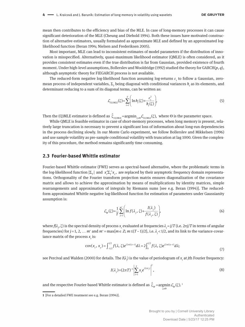


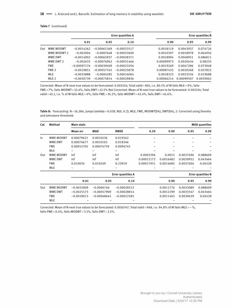
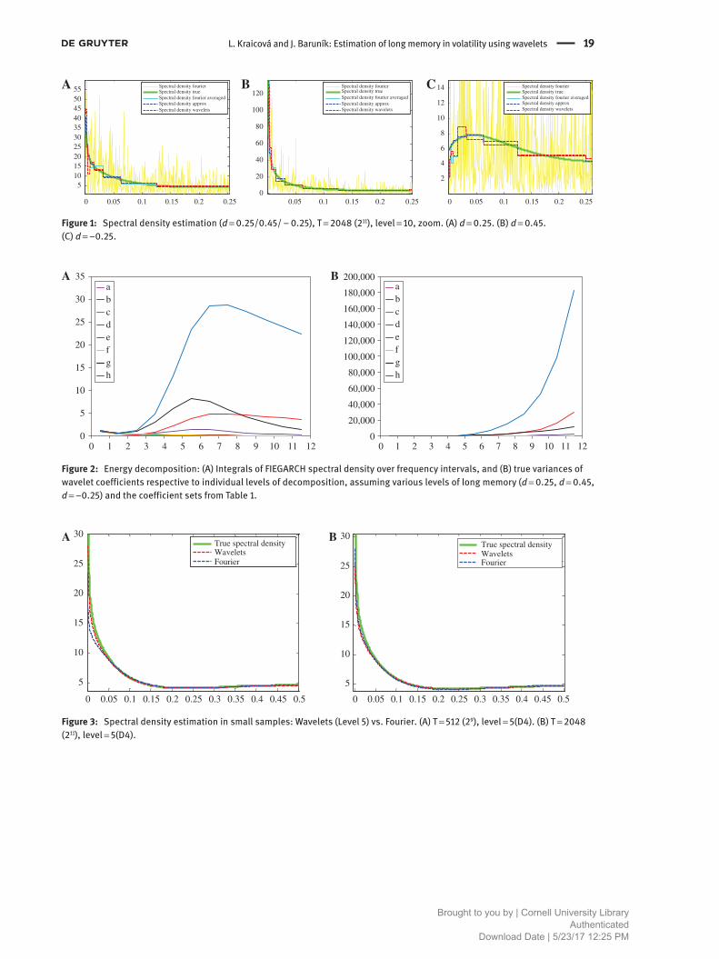


![E jozef colpaert_lyon2010_colpaert[1]](https://static.documents.pub/doc/80x56/55951a621a28ab2f5e8b46eb/e-jozef-colpaertlyon2010colpaert1.jpg)


