261

PhD THESIS / TESIS DOCTORAL
Cloud screening algorithm for MERIS and CHRIS
multispectral sensors
Luis Gomez Chova
Thesis Advisors / Directores de Tesis
Dr. Javier Calpe Maravilla
Dr. Gustavo Camps i Valls
Dept. Enginyeria Electronica. Escola Tecnica Superior d’Enginyeria.
UNIVERSITAT DE VALENCIA – ESTUDI GENERAL
Valencia – Septiembre, 2008.

Cloud screening algorithm for MERIS and CHRIS multispectral sensors
Luis Gomez Chova, 2008.
Copyright c© 2008 Luis Gomez Chova. All rights reserved.
Book cover art by Luis Gomez Chova. The picture shows the cloud mask generated by the
algorithm presented in this Thesis for an ENVISAT/MERIS multispectral image acquired over
The Netherlands in 2003 (ESA).

Agradecimientos
La senda es sinuosa y el camino es largo. Quiero suponer que por eso, y por mi promiscuidad
cientıfica, terminar esta Tesis me ha llevado mas tiempo del deseable (la salud mental es lo
primero), del establecido por los canones (becas y plazas predoctorales de 4 anos), y del aconsejable
(en Espana, en la carrera docente universitaria, el que llega el ultimo . . . se lo pierde). Sin embargo,
nunca he querido verlo de ese modo (tal vez nunca tuve el tiempo suficiente para pararme a
pensarlo) y he intentado disfrutar y aprender con cada una de las cosas que he hecho.
En este proceso, una de las personas que me ha acompanado siempre es mi director de Tesis:
el Dr. Javier Calpe Maravilla. Quiero hacer notar que introduzco de manera formal a todos los
doctores que menciono en los agradecimientos por lo presente que tengo el esfuerzo requerido para
obtener el grado de doctor y para animar a los que aun no lo tienen. No obstante, en el caso
del Dr. Javier Calpe, uno de sus grandes meritos es el de ser simplemente Javi, ya que comenzo
siendo un magnıfico guıa, paso a ser un gran colega y amigo, y creo que siempre sera un ejemplo
en el que reflejarse. Todos estos calificativos son aplicables tambien al Dr. Gustavo Camps Valls
(Gus) que, durante los primeros pasos de mi investigacion y desinteresadamente, me proporciono
su esfuerzo e interes; los cuales le agradecı incluyendole a traicion como director de mi Tesis;
lo cual me agradecio el a mi introduciendome en el maravilloso mundo de los kernels (los que
continuen mas alla de los agradecimientos y acaben leyendo la Tesis entenderan mejor la ironıa).
Encontrarse con dos directores de Tesis tan trabajadores y excelentes en general puede que
parezca el elogio tıpico de unos agradecimientos de Tesis, pero no lo es. Como tampoco lo es
la calidad personal del resto de miembros del Grupo de Procesado Digital de Senales (GPDS)
del Departamento de Ingenierıa Electronica. Agradecerles a todos el impresionante entorno de
trabajo y companerismo mostrado desde el primer dıa. Tras el tiempo que llevo con ellos (Antonio,
Alfredo, Emilio, Emma, Gus, Javi, Joan, Jose, Jordi, Jovi, Juan, Juanito, Julia, Manolo, Marsel,
Rafa), me resultarıa difıcil destacar a algunos de ellos en el plano personal, por lo que me limito
a destacar las contribuciones directas o indirectas a esta Tesis: al Dr. Emilio Soria (Emilio) y Dr.
Jose David Martın (Joseba) que, ademas de demostrar que la Tesis podıa ser leıda, la revisaron;
al Dr. Jordi Munoz (Jordi) que mantuvo a raya a matrix; al Dr. Marcelino Martınez (Marsel) que
siempre equilibro la balanza Tesis/docencia a mi favor; y a Joan y Julia (a sacarse el doctorado
rapidito si quereis algo mas) que me han soportado estos anos y han compartido lo bueno y lo
malo con alegrıa.
iii

Dado el caracter interdisciplinar de esta Tesis, la ayuda recibida (y por tanto los corre-
spondientes agradecimientos) no ha provenido solo de personal del Departamento de Ingenierıa
Electronica. El segundo pilar de esta Tesis lo constituyen miembros del Departamento de Fısica
de la Tierra y Termodinamica. En particular, el Dr. Jose Moreno (Pepe) ha sido una figura clave
tanto como elemento inspirador de la Tesis como referencia cientıfica inestimable a lo largo de
todo el trabajo. De su mano y de la del Dr. Javier Calpe se inicio una colaboracion en el campo
de la teledeteccion que gracias a su empuje ha producido una lınea de investigacion fructıfera y
estable. Mencion especial merecen el Dr. Luis Guanter (LuisGu) y Luis Alonso (QuasiDr.) con
quienes he aprendido a llevar la teledeteccion a la practica viendo mas alla de una matriz de datos
(a escondidas de Gus). Con ellos he experimentado la investigacion desde lo puramente teorico
en multiples publicaciones y conferencias hasta su vertiente mas aplicada en campanas de campo
y reuniones de proyecto. En todo este tiempo, tanto los lazos profesionales como afectivos no han
hecho mas que crecer. Parafraseando al Dr. Luis Guanter (2006) hago mıa su premonitoria frase
“Ya llevamos bastantes batallas juntos, y por mi parte que no se acaben nunca”.
En todo proceso de aprendizaje, es tan bueno rodearse de gente competente en el dıa a dıa como
conocer nuevos puntos de vista y formas de trabajar. En este aspecto, han sido importantısimas
las experiencias vividas en las estancias predoctorales en el extranjero. Quiero agradecer al Dr.
Diego Fernandez Prieto del European Space Research Institute (ESRIN) of the European Space
Agency (ESA) el tiempo que me dedico, dandome la oportunidad de tener un primer contacto con
la Agencia Espacial Europea y la inolvidable experiencia de vivir en Frascati y la Citta Eterna.
Al Dr. Andreas Muller, a Martin Habermeyer y a todo el grupo de Imaging Spectroscopy del
German Aerospace Center (DLR) en Munchen (quien me iba a decir que la Oktoberfest era en
septiembre). Por ultimo (cronologicamente), agradecer al Dr. Lorenzo Bruzzone de la Universita
Degli Studi di Trento su amistad y su contribucion a mi investigacion. Sin olvidar al resto de
miembros del Remote Sensing Laboratory (Claudio, Michele, Mattia e Silvia) y en especial a la
Dr. Francesca Bovolo que tambien ha sufrido la elaboracion de esta Tesis.
Hacer constar tambien que todo este trabajo no habrıa sido posible sin el apoyo y financiacion
(el tiempo requerido por una Tesis no permite dedicarse a esto sin algo de vil metal) del Ministerio
de Educacion y Ciencia con la beca predoctoral FPU y a la Universitat de Valencia que me permitio
compaginar la conclusion de la Tesis con el trabajo de profesor ayudante. Tambien agradecer a la
Agencia Espacial Europea su labor en el campo de la Observacion de la Tierra que ha permitido la
adquisicion de los datos en los que se basa este trabajo y su activa financiacion de la investigacion
cientıfica que a contribuido a la mejor consecucion de los objetivos planteados. Y hablando de
Tesis doctorales y datos adquiridos, debo recordar tambien a mi colega y amigo Raul Zurita Milla
(futuro doctor dentro de 15 dıas) y a sus directores de Tesis Dr. Jan Clevers y Dr. Michael
Schaepman de la Wageningen University. A ellos debo agradecerles que me proporcionasen la
serie temporal de imagenes de MERIS adquiridas sobre Los Paıses Bajos en el 2003 que se ha
empleado en esta Tesis y tambien que me indujesen a escudrinar los datos de MERIS a nivel
subpixel.

Dejo para el final a todos aquellos que no han intervenido en los detalles de esta Tesis pero que
son responsables del resultado en su conjunto. Ellos son la base sobre la que construyo mi vida y
a ellos les dedico este trabajo ya que lo hacen posible. A mis amigos, que me bajan del satelite
y me permiten observar la Tierra desde el suelo. Para que siga observandola y disfrutandola con
vosotros: David, Inma, Agustın (vuelve ya), Lorda, Javi, Nacho, Marıa, con todos. A mi familia.
A mi hermano, que me enseno la constancia necesaria para conseguir cosas como esta Tesis. A
mi abuela, que me ensena dıa a dıa. A mis padres, que me lo ensenaron todo. A Norma, que me
enseno a querer.
Luis Gomez Chova
Valencia, 2008

“It is better to remain silent and be thought a fool,
than to open your mouth and remove all doubt.”
attr to George Eliot (Mary Ann Evans)

Contents
Abstract xi
Overview xiii
I Introduction 1
1 Remote Sensing from Earth Observation Satellites 3
1.1 Electromagnetic Radiation and Radiative Transfer . . . . . . . . . . . . . . . . . . 4
1.1.1 Electromagnetic Radiation . . . . . . . . . . . . . . . . . . . . . . . . . . . 4
1.1.2 Solar Irradiance . . . . . . . . . . . . . . . . . . . . . . . . . . . . . . . . . . 4
1.1.3 Earth Atmosphere . . . . . . . . . . . . . . . . . . . . . . . . . . . . . . . . 7
1.1.4 At-Sensor Radiance . . . . . . . . . . . . . . . . . . . . . . . . . . . . . . . 9
1.2 Multispectral and Hyperspectral Imaging Spectrometers . . . . . . . . . . . . . . . 15
1.3 Push-broom Imaging Spectrometers . . . . . . . . . . . . . . . . . . . . . . . . . . 17
1.3.1 The MEdium Resolution Imaging Spectrometer (MERIS) . . . . . . . . . . 20
1.3.2 The Compact High Resolution Imaging Spectrometer (CHRIS) . . . . . . . 22
1.4 Motivation . . . . . . . . . . . . . . . . . . . . . . . . . . . . . . . . . . . . . . . . 25
2 Cloud Screening from Earth Observation Images 27
2.1 Cloud Types and Characteristics . . . . . . . . . . . . . . . . . . . . . . . . . . . . 28
2.2 Clouds and the Energy Cycle . . . . . . . . . . . . . . . . . . . . . . . . . . . . . . 31
2.3 Cloud Properties . . . . . . . . . . . . . . . . . . . . . . . . . . . . . . . . . . . . . 33
2.4 Review of Cloud Screening Algorithms . . . . . . . . . . . . . . . . . . . . . . . . . 35
2.4.1 Reference Cloud Screening Algorithms . . . . . . . . . . . . . . . . . . . . . 37
vii

II Methodology for Cloud Identification 41
3 Proposed Methodology for Cloud Screening 43
4 Image Pre-processing and Feature Extraction 47
4.1 Pre-processing (I): TOA Radiance Corrections . . . . . . . . . . . . . . . . . . . . 47
4.1.1 Corrections for MERIS . . . . . . . . . . . . . . . . . . . . . . . . . . . . . 48
4.1.2 Corrections for CHRIS . . . . . . . . . . . . . . . . . . . . . . . . . . . . . . 49
4.2 Pre-processing (II): TOA Reflectance . . . . . . . . . . . . . . . . . . . . . . . . . . 64
4.2.1 Day-of-Year Correction . . . . . . . . . . . . . . . . . . . . . . . . . . . . . 64
4.2.2 Rough Surface Correction . . . . . . . . . . . . . . . . . . . . . . . . . . . . 66
4.3 Feature Extraction . . . . . . . . . . . . . . . . . . . . . . . . . . . . . . . . . . . . 67
4.3.1 Surface Spectral Features . . . . . . . . . . . . . . . . . . . . . . . . . . . . 68
4.3.2 Atmospheric Features . . . . . . . . . . . . . . . . . . . . . . . . . . . . . . 70
4.3.3 Remarks on CHRIS Acquisition Modes . . . . . . . . . . . . . . . . . . . . 75
5 Unsupervised Cloud Classification 77
5.1 Pixel Identification and ROI Selection . . . . . . . . . . . . . . . . . . . . . . . . . 77
5.1.1 Water/Land Identification . . . . . . . . . . . . . . . . . . . . . . . . . . . . 77
5.1.2 Region of Interest with Cloud Covers . . . . . . . . . . . . . . . . . . . . . . 79
5.2 Unsupervised Classification with the EM Algorithm . . . . . . . . . . . . . . . . . 79
5.2.1 EM Algorithm . . . . . . . . . . . . . . . . . . . . . . . . . . . . . . . . . . 79
5.2.2 Cloud Identification . . . . . . . . . . . . . . . . . . . . . . . . . . . . . . . 82
5.3 Cloud Abundance . . . . . . . . . . . . . . . . . . . . . . . . . . . . . . . . . . . . . 84
5.3.1 Linear Spectral Unmixing . . . . . . . . . . . . . . . . . . . . . . . . . . . . 84
5.3.2 Cloud Abundance fraction . . . . . . . . . . . . . . . . . . . . . . . . . . . . 85
5.3.3 Cloud Final Product . . . . . . . . . . . . . . . . . . . . . . . . . . . . . . . 86
6 Semi-supervised Cloud Classification 89
6.1 Introduction to Kernel Methods . . . . . . . . . . . . . . . . . . . . . . . . . . . . . 91
6.1.1 Learning from Samples, Regularization, and Kernel feature space . . . . . . 91
6.1.2 Support Vector Machines . . . . . . . . . . . . . . . . . . . . . . . . . . . . 93
6.1.3 Composite Kernels Framework . . . . . . . . . . . . . . . . . . . . . . . . . 95
6.2 Semi-supervised Classification with the Laplacian SVM . . . . . . . . . . . . . . . 99
6.2.1 Manifold Regularization Learning Framework . . . . . . . . . . . . . . . . . 100
6.2.2 Laplacian Support Vector Machines . . . . . . . . . . . . . . . . . . . . . . 101
6.2.3 Remarks on Laplacian SVM . . . . . . . . . . . . . . . . . . . . . . . . . . . 104
6.3 Semi-supervised Classification with Composite Mean Kernels . . . . . . . . . . . . 104
6.3.1 Image Clustering . . . . . . . . . . . . . . . . . . . . . . . . . . . . . . . . . 106
6.3.2 Cluster Similarity and the Mean Map . . . . . . . . . . . . . . . . . . . . . 106
6.3.3 Composite Pixel-Cluster Kernels . . . . . . . . . . . . . . . . . . . . . . . . 108
6.3.4 Sample Selection Bias and the Soft Mean Map . . . . . . . . . . . . . . . . 110
6.3.5 Summary of Composite Mean Kernel Methods . . . . . . . . . . . . . . . . 112
6.3.6 Performance on Synthetic Data . . . . . . . . . . . . . . . . . . . . . . . . . 113
6.4 Remarks on Semi-supervised Cloud Classification . . . . . . . . . . . . . . . . . . . 118
III Experimental Results 121
7 Unsupervised Cloud Screening Validation 123
7.1 Visual Inspection of PROBA/CHRIS Images . . . . . . . . . . . . . . . . . . . . . 125
7.1.1 CHRIS Sample Products . . . . . . . . . . . . . . . . . . . . . . . . . . . . 125
7.1.2 CHRIS Cloud Screening Results . . . . . . . . . . . . . . . . . . . . . . . . 126
7.2 Visual Inspection of ENVISAT/MERIS Images . . . . . . . . . . . . . . . . . . . . 128
7.2.1 MERIS Sample Products . . . . . . . . . . . . . . . . . . . . . . . . . . . . 128
7.2.2 MERIS Cloud Screening Results . . . . . . . . . . . . . . . . . . . . . . . . 129
7.3 Comparison with MERIS Standard Products . . . . . . . . . . . . . . . . . . . . . 131
7.4 Multitemporal Validation on MERIS Series . . . . . . . . . . . . . . . . . . . . . . 132
7.4.1 MERIS Time Series over The Netherlands . . . . . . . . . . . . . . . . . . . 132
7.4.2 Temporal Cloud Screening based on Change Detection . . . . . . . . . . . . 135
7.4.3 Spectral Unmixing of Multitemporal Series . . . . . . . . . . . . . . . . . . 139
7.5 The Cloud Abundance Product . . . . . . . . . . . . . . . . . . . . . . . . . . . . . 142
8 Semi-supervised Cloud Screening Validation 145

8.1 Experimental Setup . . . . . . . . . . . . . . . . . . . . . . . . . . . . . . . . . . . 146
8.2 Kernel Methods and Model Development . . . . . . . . . . . . . . . . . . . . . . . 149
8.3 Semi-supervised Cloud Screening Validation Results . . . . . . . . . . . . . . . . . 151
8.3.1 Single-Image Approach Results . . . . . . . . . . . . . . . . . . . . . . . . . 151
8.3.2 Image-Fold Approach Results . . . . . . . . . . . . . . . . . . . . . . . . . . 155
8.4 Comparison with MERIS Standard Products . . . . . . . . . . . . . . . . . . . . . 158
8.5 Results on MERIS Temporal Series . . . . . . . . . . . . . . . . . . . . . . . . . . . 162
8.6 On the Relative Importance of Labeled and Unlabeled Samples . . . . . . . . . . . 168
IV Conclusions 171
9 Discussion and Conclusions 173
9.1 Summary and Conclusions . . . . . . . . . . . . . . . . . . . . . . . . . . . . . . . . 173
9.2 Further Work . . . . . . . . . . . . . . . . . . . . . . . . . . . . . . . . . . . . . . . 180
9.3 Achievements and Relevance . . . . . . . . . . . . . . . . . . . . . . . . . . . . . . 181
9.4 Acknowledgements . . . . . . . . . . . . . . . . . . . . . . . . . . . . . . . . . . . . 183
V Appendices 189
A Acronyms 191
B List of Notational Symbols 197
VI Summary in Spanish 199
VII References 223
References 225
Abstract
Earth Observation systems monitor our Planet by measuring, at different wavelengths, the
electromagnetic radiation that is reflected by the surface, crosses the atmosphere, and reaches the
sensor at the satellite platform. In this process, clouds are one of the most important compo-
nents of the Earth’s atmosphere affecting the quality of the measured electromagnetic signal and,
consequently, the properties retrieved from these signals. This Thesis faces the challenging prob-
lem of cloud screening in multispectral and hyperspectral images acquired by space-borne sensors
working in the visible and near-infrared range of the electromagnetic spectrum. The main objec-
tive is to provide new operational cloud screening tools for the derivation of cloud location maps
from these sensors’ data. Moreover, the method must provide cloud abundance maps –instead
of a binary classification– to better describe clouds (abundance, type, height, subpixel coverage),
thus allowing the retrieval of surface biophysical parameters from satellite data acquired over
land and ocean. In this context, this Thesis is intended to support the growing interest of the
scientific community in two multispectral sensors on board two satellites of the European Space
Agency (ESA). The first one is the MEdium Resolution Imaging Spectrometer (MERIS), placed
on board the biggest environmental satellite ever launched, ENVISAT. The second one is the
Compact High Resolution Imaging Spectrometer (CHRIS) hyperspectral instrument, mounted on
board the technology demonstration mission PROBA (Project for On-Board Autonomy). The
proposed cloud screening algorithm takes advantage of the high spectral and radiometric resolu-
tion of MERIS, and of the high number of spectral bands of CHRIS, as well as the specific location
of some bands (e.g., oxygen and water vapor absorption bands) to increase the cloud detection
accuracy. To attain this objective, advanced pattern recognition and machine learning techniques
to detect clouds are specifically developed in the frame of this Thesis. First, a feature extraction
based on meaningful physical facts is carried out in order to provide informative inputs to the
algorithms. Then, the cloud screening algorithm is conceived trying to make use of the wealth
of unlabeled samples in Earth Observation images, and thus unsupervised and semi-supervised
learning methods are explored. Results show that applying unsupervised clustering methods over
the whole image allows us to take advantage of the wealth of information and the high degree of
spatial and spectral correlation of the image pixels, while semi-supervised learning methods offer
the opportunity of exploiting also the available labeled samples.

xii
Overview
Earth Observation (EO) covers those procedures and scientific methodologies focused on mon-
itoring our Planet by means of electromagnetic radiation sensors located on space-borne or air-
borne platforms. The information these sensors provide represents spatial and temporal scales
completely different to those obtained from ground measurements. Particularly, optical passive
remote sensing lies on the study of the surface by means of the solar radiation reflected by the
observed target and transmitted through the atmosphere to the sensor.
Materials in a scene reflect, absorb, and emit electromagnetic radiation in different ways
depending on their molecular composition and shape. Remote sensing exploits this physical fact
and deals with the acquisition of information about a scene at a short, medium, or long distance.
The radiation acquired by a sensor is measured at different wavelengths, and the resulting spectral
signature (or spectrum) is used to identify a given material or to retrieve surface biophysical
parameters from it. The field of spectroscopy is concerned with the measurement, analysis, and
interpretation of such spectra.
However, EO from remote sensing data implies accounting for the coupling between atmo-
sphere and surface radiative effects. If there were no atmosphere around the Earth, the solar
radiation would only be perturbed when it reached the surface. Therefore, incoming radiation
would provide a direct representation of the surface nature and the associated dynamics when
registered by a space-borne sensor. Nevertheless, the atmospheric influence on the visible (VIS)
and infrared (IR) radiation is strong enough to modify the reflected electromagnetic signal, caus-
ing the loss or corruption of part of the carried information. The interaction of the solar radiation
with the atmospheric components consists of absorption and scattering processes. The absorption
decreases the intensity of the radiation arriving at the sensor, which causes a loss of the brightness
of the target, while the scattering mainly acts modifying the propagation direction.
In this scenario, clouds are one of the most important components of Earth’s atmosphere, and
constitute the core focus of this work. The presence of clouds affects dramatically the quality
and reliability of the measured electromagnetic signal and thus the retrieved surface properties.
The corresponding cloud influence depends on the cloud type, cloud cover, cloud height, and
cloud distribution in the sky. For instance, thick opaque clouds impede the incoming radiation
reaching the surface, while thin transparent clouds contaminate the data with photons scattered
in the observation direction or attenuates the signal by the removal of photons in their travel to
the sensor. As a result, any set of remote sensing images needs for cloud screening in the initial
processing steps before exploiting the data to ensure a maximal accuracy in the results. This is
the fundamental basis of cloud screening in optical remote sensing: the detection of the clouds in
the observer’s line of sight in order to identify the usefulness of the signal reflected by the target.
Accurate identification of clouds in remote sensing images is a key issue for a wide range of
remote sensing applications, especially in the case of sensors working in the visible and near-
infrared (VNIR) range of the electromagnetic spectrum. The amount of images acquired over the
globe every day by the instruments on board EO satellites makes inevitable that many of these
images present cloud covers, whose extent depends on the season and the geographic position of
the study region. It is estimated that more than 60% of the globe is covered by clouds. Therefore,
from an operational point of view, undetected clouds are the most significant source of error for
ground reflectance retrieval, affecting a wide range of remote sensing applications.
One the one hand, clouds can be viewed as a source of contamination that makes the image
partly useless for assessing landscape properties. Without an accurate cloud masking, undetected
clouds in the scene are the most significant source of error for true ground reflectance estimation,
and thus for biophysical parameter retrieval over both water and land covers. By masking only
those image areas affected by cloud covers, the whole image must not be necessarily discarded,
increasing usability of remote sensing data or making multitemporal studies possible. On the
other hand, global scale monitoring of clouds is a key requirement for an adequate modeling
of the Earth’s climate. Having a global scale monitoring of clouds is becoming more and more
important in climatological aspects: clouds contribute significantly to the global radiation budget
with its role in the direct radiative forcing, and thin clouds are responsible for the atmospheric
greenhouse effect. Therefore, clouds can be viewed as a source of contamination that makes
the image partly useless for assessing landscape properties, or as a source of information for
measuring important climatological parameters. In both cases, an automatic and accurate method
for cloud screening in optical remote sensing is required. As a result, cloud screening represents
an important preprocessing task for any EO image in order to ensure a maximal accuracy and
reliability in the results inferred by the latter exploitation of the data.
Under the light of the aforementioned needs and demands, the present Thesis addresses the
crucial problem in the remote sensing of environment of developing an operational, accurate and
automated set of tools for the discrimination of clouds. We can clearly state different objectives
in this work:
1. To analyze the problem of cloud detection under different perspectives. The intrinsic multi-
disciplinary nature of this work (in the intersect of Physics, Thermodynamics, Telecom-
munications, Computer Science and Machine Learning) will allow us to extract different
features for better understanding and modeling the problem.
2. To better understand signals provided by ENVISAT/MERIS (Rast et al., 1999) and PROBA
xiv

/CHRIS (Barnsley et al., 2004) imaging spectrometers. In particular, PROBA is a tech-
nology demonstration satellite whose sensor CHRIS provides minimally preprocessed data.
Appropriate correction and calibration of CHRIS and MERIS data is a key issue for accurate
cloud screening and also for other remote sensing applications.
3. To develop an automatic, robust and operational algorithm for cloud screening. The algo-
rithm should primarily provide a cloud mask interpretable as cloud abundance.
4. To validate the proposed algorithm extensively. This is achieved through two different ways:
comparing the resulting cloud masks with the official MERIS and CHRIS products and with
the multi-temporal classification of cloud-covered image series.
5. To provide the remote sensing community with a set of guidelines and recommendations for
developing further missions and satellite sensors.
This Thesis is organized in four different parts: (1) a thorough literature review, (2) the devel-
opment of a set of robust tools for automated cloud screening, (3) the evaluation of the proposed
algorithms in real situations, and (4) the elaboration of a set of guidelines and recommendations
aimed to be useful for further missions:
Part I reviews the fundamental basis of passive remote sensing, cloud physical and optical prop-
erties, along with a compilation of state-of-the-art cloud screening methods. This first step
identifies strengths and weaknesses of the most representative algorithms to date.
Part II addresses the proposed methodology for cloud product generation. In particular, to
obtain cloud probability masks and knowledge from the extracted cloud features.
Part III deals with the validation of the proposed methodology and cloud products. A wide
database of images has been included in the study in order to take into account their
different characteristics: type of cloud (cumulus, cirrus, stratocumulus); geographic location
(latitude/longitude); date (season); and surface types. The validation of cloud detection
algorithms is not an easy task because there is no independent measurement with the same
spatial resolution. For this reason, significant effort has to be done in order to validate
results by using different techniques.
Part IV summarizes the accomplished objectives, discusses the main conclusions, and provides
guidelines and recommendations to improve cloud screening for multispectral imaging spec-
trometers in future EO missions.
xv

xvi

Part I
Introduction


Chapter 1
Remote Sensing from Earth
Observation Satellites
Passive optical remote sensing relies on solar radiation as the source of illumination. This
solar radiation travels across the Earth atmosphere before being reflected by the surface and
again before arriving at the sensor. Thus, the signal measured at the satellite is the emergent
radiation from the Earth surface-atmosphere system in the sensor observation direction.
The reflectance of the observed target should be the parameter of interest since it characterizes
the surface independently of atmospheric effects and seasonal and diurnal differences in solar
position. However, the estimation of the surface reflectance from the radiance measured at the
satellite –also known as atmospheric correction– requires an accurate estimation of the parameters
used to model the atmospheric effects and then to compensate them using a proper radiative
transfer model. The main problem is that, radiative transfer modeling for surface reflectance
retrieval assumes cloud-free data in order to estimate atmospheric parameters from the data
themselves. Thus, results over clouds have no physical interpretation and a previous accurate
cloud screening is required. Hence, cloud screening is the first processing step after noise reduction
and radiometric calibration.
We must state here that atmospheric correction procedure is out of the scope of this Thesis.
Nevertheless, since cloud screening is carried out before the atmospheric correction is done, inter-
action between the atmosphere and the radiation will be taken into account in order to quantify
the atmospheric effects on the measured signal. Moreover, an accurate formulation of the atmo-
spheric effects on the retrieved signal allows us to estimate useful features to discriminate clouds
from surface.
In this chapter, a brief introduction to the solar electromagnetic radiation and its interaction
with the Earth atmosphere is given. The absorption and scattering processes affecting the solar
electromagnetic radiation in its path across the atmosphere until reaching the sensor are described.
The acquisition and operation mode of common multispectral imaging spectrometers is detailed.
Chapter 1. Remote Sensing from Earth Observation Satellites
Finally, a brief description of ENVISAT/MERIS and PROBA/CHRIS satellite sensors is included
together with discussion about current opportunities and identified problems that justify the
selection of these sensors and cloud screening to be studied in the present Thesis.
1.1 Electromagnetic Radiation and Radiative Transfer
1.1.1 Electromagnetic Radiation
Electromagnetic radiation (EMR) travels through space in the form of periodic disturbances
of electric and magnetic fields that simultaneously oscillate in planes mutually perpendicular
to each other and to the direction of propagation through space at the speed of light (c =
2.99792458 × 10⁸ m/s). The electromagnetic spectrum is a continuum of all electromagnetic
waves arranged according to frequency or wavelength, which are defined as the number of wave
peaks passing a given point per second and the distance from peak to peak, respectively. Thus,
both frequency, ν (Hz), and wavelength, λ (m), of an EMR wave are related by its propagation
speed, c = λν. The energy carried by EMR is contained in the photons that travel as a wave,
being the energy in a photon proportional to the frequency, E = hν = ~ω, where h is the Planck’s
constant (h = 6.626 × 10⁻³⁴ J s) and ~ = h/2π is called the reduced Planck’s constant.
The spectrum is divided into regions based on wavelength ranging from short gamma rays,
which have wavelengths of 10−6 µm or less, to long radio waves which have wavelengths of many
kilometers. Since the range of electromagnetic wavelengths is so vast, the wavelengths are often
shown graphically on a logarithmic scale (see Fig. 1.1 for a detailed classification of the electro-
magnetic spectrum). Visible light is composed of wavelengths ranging from 400 to 700 nm, i.e.
from blue to red. This narrow portion of the spectrum is the entire range of the electromag-
netic energy to which the human visual system is sensitive to. When viewed through a prism,
this range of the spectrum produces a rainbow, that is, a spectral decomposition in fundamental
harmonics or frequency components (colors). Just beyond the red-end of the visible (VIS) region
there is the region of infrared (IR) energy waves: near-infrared (NIR), shortwave-infrared (SWIR),
middle-infrared (MIR), and the thermal-infrared (TIR).
The VIS and IR regions are commonly used in remote sensing. In particular, passive optical
remote sensing is mainly focused in the VIS and NIR spectral region (VNIR), and in the SWIR
since it depends on the Sun as the unique source of illumination. The predominant type of energy
detection in the wavelength regions from 400 to 3000 nm (VNIR and SWIR) is based on the
reflected sunlight.
1.1.2 Solar Irradiance
Energy generated by nuclear fusion in the Sun’s core is the responsible for the electromagnetic
radiation emitted by the Sun in its outer layer, which is known as the photosphere. It is the
4

1.1. Electromagnetic Radiation and Radiative Transfer
Electromagnetic
Spectrum
Microwave
Thermal
InfraredNear & Mid
Infrared
Visible
(VIS)
IRUV
Ultraviolet
X-Rays
γ-Rays
400 500 600 700 nm
Wavelength (µm) Wavelength (µm)
10 10 10 10 10 10 1 10 10 10 10 10 10 10 10-6 -5 -4 -3 -2 -1 2 3 4 5 6 7 8
TV/Radio
Figure 1.1: Electromagnetic spectrum classification based on wavelength range.
continuous absorption and emission of EMR by the elements in the photosphere that produces
the light observed emanating from the Sun. The absorption characteristics of these elements
produces variations in the continuous spectrum of solar radiation, resulting in the typical solar
irradiance spectral curve. It must be stressed that 99% of the solar radiative output occurs within
the wavelength interval 300-10000 nm.
The rate of energy transfer by EMR, the so-called radiant flux, incident per unit area is termed
the radiant flux density or irradiance (W/m2). A quantity often used in remote sensing is the
irradiance per unit wavelength, and is termed the spectral irradiance (with units W/m2/nm). The
total radiant flux from the Sun is approximately 3.84 × 1026 W and, since the mean Earth-Sun
distance is 1.496 × 10¹¹ m, the total solar irradiance, over all wavelengths, incident at the top of
the atmosphere (TOA), at normal incidence to the Earth’s surface, is
F0 =3.84 × 1026
4π(1.496 × 10¹¹)2= 1370 W/m2, (1.1.1)
which is known as the the solar constant, although it presents a considerable variation with time.
The observed variations at the Sun are due to localized events on the photosphere known as
sunspots and faculae1. An increased number of these events occurs approximately every 11 years,
a period known as the solar cycle. However, the largest source of variation in the incident solar
irradiance at the TOA is the orbit of the Earth around the Sun, due to the variable Earth-Sun
distance that varies with the day of year.
Space-borne instruments allow us measuring the spectral variation in solar irradiance at the
TOA without the effects of the Earth’s atmosphere which, depending on the wavelength of the
1Sunspots are dark areas on the photosphere which are cooler than surrounding regions. They have lifetimes
ranging from a few days to weeks and are accompanied by strong magnetic fields. Faculae are regions of the
photosphere which are hotter than their surroundings. They often occur in conjunction with sunspots and also
possess strong magnetic fields and similar lifetimes.
5
Chapter 1. Remote Sensing from Earth Observation Satellites
200 400 600 800 1000 1200 1400 1600 1800 2000 2200
0.2
0.4
0.6
0.8
1
1.2
1.4
1.6
1.8
2
wavelength (nm)
Sol
ar Ir
radi
ance
(W
/m2 /n
m)
Thuillier et al. (2003)
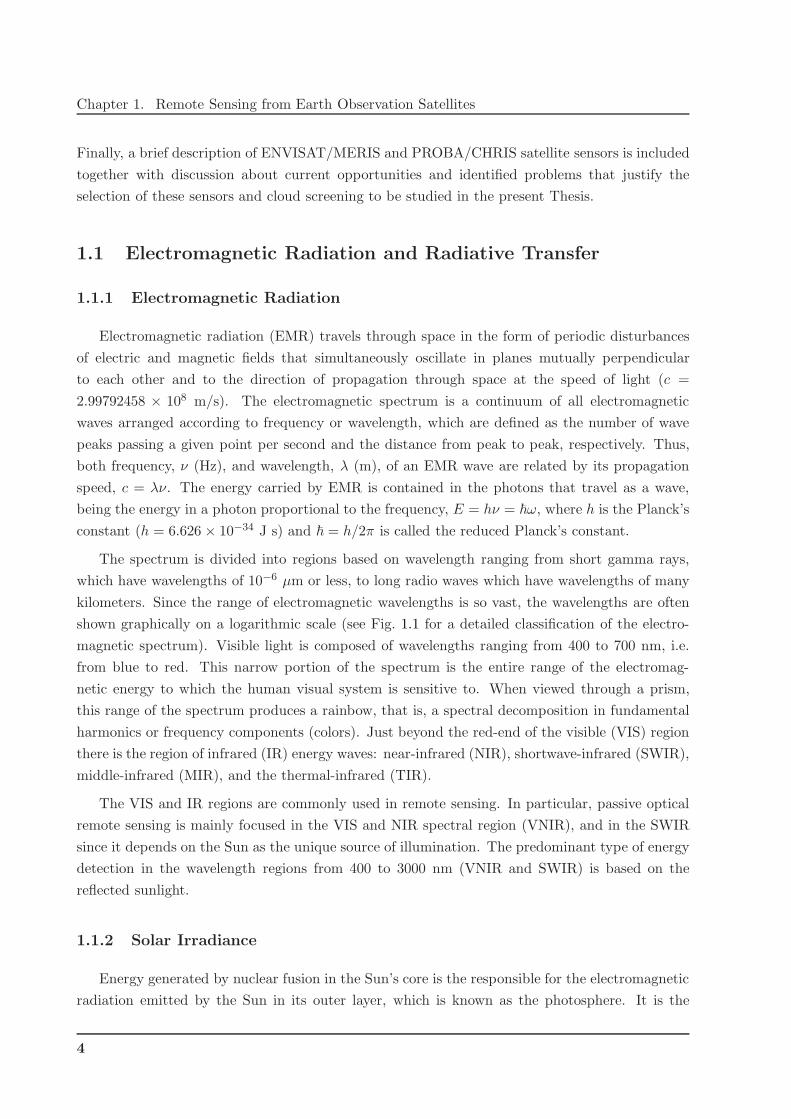
Figure 1.2: Solar spectral irradiance at the top of the Earth’s atmosphere.
radiation, can reduce the intensity of the measured radiation. In this Thesis, the used solar
spectral irradiance curve, F0(λ), comes from Thuillier et al. (2003), where the ultraviolet (UV),
visible, and infrared spectra from the ATmospheric Laboratory for Applications and Science
(ATLAS) and the EUropean Retrieval CArrier (EURECA) missions were merged into a single
absolute solar irradiance spectrum covering the 200 to 2400 nm range. In particular, the SOLar
SPECtrum (SOLSPEC) and the SOlar SPectrum (SOSP) spectrometers, on board ATLAS and
EURECA missions respectively, were used to carry out the solar spectral irradiance measurements.
Figure 1.2 shows the solar spectral irradiance at the top of the Earth’s atmosphere (Thuillier et al.,
2003).
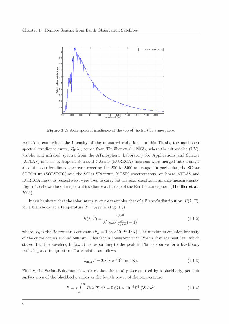
It can be shown that the solar intensity curve resembles that of a Planck’s distribution, B(λ, T ),
for a blackbody at a temperature T = 5777 K (Fig. 1.3):
B(λ, T ) =2~c2
λ5(exp( ~ckBTλ) − 1)
, (1.1.2)
where, kB is the Boltzmann’s constant (kB = 1.38×10⁻²³ J/K). The maximum emission intensity
of the curve occurs around 500 nm. This fact is consistent with Wien’s displacement law, which
states that the wavelength (λmax) corresponding to the peak in Planck’s curve for a blackbody
radiating at a temperature T are related as follows:
λmaxT = 2.898 × 10⁶ (nm K). (1.1.3)
Finally, the Stefan-Boltzmann law states that the total power emitted by a blackbody, per unit
surface area of the blackbody, varies as the fourth power of the temperature:
F = π
∫ ∞
0B(λ, T )dλ = 5.671 × 10⁻⁸T 4 (W/m2) (1.1.4)
6
1.1. Electromagnetic Radiation and Radiative Transfer
100 1000 10000 10000010
−4
10−2
100
102
104
106
Sun (5777K)
Lava (1400K)
Forest Fire(900K)
Ambient(300K) Artic Ice
(220K)
wavelength (nm)
Rel
ativ
e S
pect
ral R
adia
nce
Figure 1.3: Blackbody emission of objects at typical temperatures.
Because the Sun and Earth’s spectra have a very small overlap (Fig. 1.3), the radiative transfer
processes for solar and infrared regions are often considered as two independent problems.
1.1.3 Earth Atmosphere
The Earth’s surface is covered by a layer of atmosphere consisting of a mixture of gases and
other solid and liquid particles. The principal gaseous constituents, present in nearly constant
concentration, are nitrogen (78%), oxygen (21%), argon (1%), and-minor constituents (<0.04%).
Water vapor and an ozone layer are also present. The atmosphere also contains solid and liquid
particles such as aerosols, water droplets (clouds or raindrops), and ice crystals (snowflakes).
These particles may aggregate to form clouds and haze.
The vertical profile of the atmosphere is divided into four main layers: troposphere, strato-
sphere, mesosphere, and thermosphere. The tops of these layers are known as the tropopause
(10 km), stratopause (50 km), mesopause (85 km), and thermopause, respectively. The gaseous
materials extend to several hundred kilometers in altitude, though there is no well-defined limit
of the atmosphere.
All the weather activities (water vapour, clouds, precipitation) are confined to the troposphere.
A layer of aerosol particles normally exists near to the Earth’s surface, and the aerosol concen-
tration decreases nearly exponentially with height, with a characteristic height of about 2 km. In
fact, the troposphere and the stratosphere together (first 30 km of the atmosphere) account for
more than 99% of the total mass of the Earth’s atmosphere. Finally, ozone exists mainly at the
stratopause.
The characteristic difference between molecules and aerosols in the atmosphere is their respec-
tive size or radius (D’Almeida et al., 1991). Molecules have a radius on the order of 0.1 nm, while
7
Chapter 1. Remote Sensing from Earth Observation Satellites
0.3 0.5 1.0 1.5 3.0 5.0 10.0 15.0 20.02.0
0
100
SWIRUV VIS MIRII TIR FIRNIR I
wavelength (µm)
Tra
nsm
issio
n[%
]
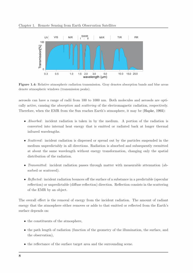
Figure 1.4: Relative atmospheric radiation transmission. Gray denotes absorption bands and blue areas
denote atmospheric windows (transmission peaks).
aerosols can have a range of radii from 100 to 1000 nm. Both molecules and aerosols are opti-
cally active, causing the absorption and scattering of the electromagnetic radiation, respectively.
Therefore, when the EMR from the Sun reaches Earth’s atmosphere, it may be (Hapke, 1993):
• Absorbed : incident radiation is taken in by the medium. A portion of the radiation is
converted into internal heat energy that is emitted or radiated back at longer thermal
infrared wavelengths.
• Scattered : incident radiation is dispersed or spread out by the particles suspended in the
medium unpredictably in all directions. Radiation is absorbed and subsequently reemitted
at about the same wavelength without energy transformation, changing only the spatial
distribution of the radiation.
• Transmitted : incident radiation passes through matter with measurable attenuation (ab-
sorbed or scattered).
• Reflected : incident radiation bounces off the surface of a substance in a predictable (specular
reflection) or unpredictable (diffuse reflection) direction. Reflection consists in the scattering
of the EMR by an object.
The overall effect is the removal of energy from the incident radiation. The amount of radiant
energy that the atmosphere either removes or adds to that emitted or reflected from the Earth’s
surface depends on:
• the constituents of the atmosphere,
• the path length of radiation (function of the geometry of the illumination, the surface, and
the observation),
• the reflectance of the surface target area and the surrounding scene.
8
1.1. Electromagnetic Radiation and Radiative Transfer
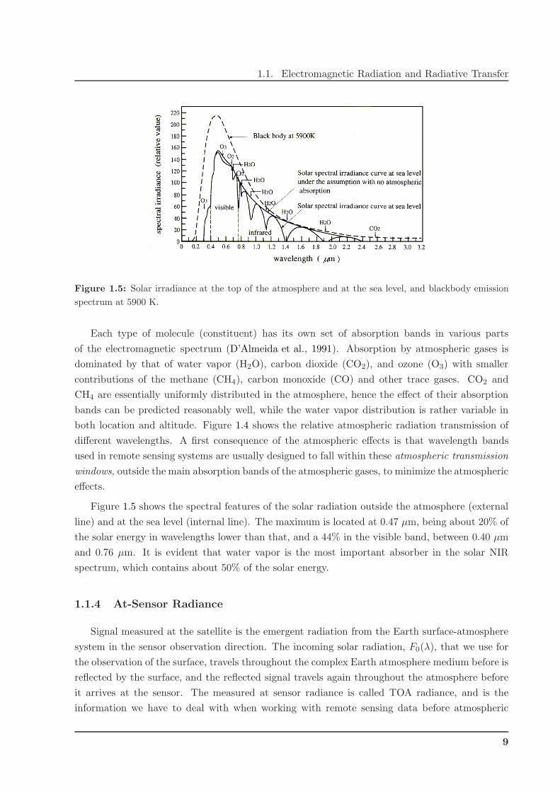
Figure 1.5: Solar irradiance at the top of the atmosphere and at the sea level, and blackbody emission
spectrum at 5900 K.
Each type of molecule (constituent) has its own set of absorption bands in various parts
of the electromagnetic spectrum (D’Almeida et al., 1991). Absorption by atmospheric gases is
dominated by that of water vapor (H2O), carbon dioxide (CO2), and ozone (O3) with smaller
contributions of the methane (CH4), carbon monoxide (CO) and other trace gases. CO2 and
CH4 are essentially uniformly distributed in the atmosphere, hence the effect of their absorption
bands can be predicted reasonably well, while the water vapor distribution is rather variable in
both location and altitude. Figure 1.4 shows the relative atmospheric radiation transmission of
different wavelengths. A first consequence of the atmospheric effects is that wavelength bands
used in remote sensing systems are usually designed to fall within these atmospheric transmission
windows, outside the main absorption bands of the atmospheric gases, to minimize the atmospheric
effects.
Figure 1.5 shows the spectral features of the solar radiation outside the atmosphere (external
line) and at the sea level (internal line). The maximum is located at 0.47 µm, being about 20% of
the solar energy in wavelengths lower than that, and a 44% in the visible band, between 0.40 µm
and 0.76 µm. It is evident that water vapor is the most important absorber in the solar NIR
spectrum, which contains about 50% of the solar energy.
1.1.4 At-Sensor Radiance
Signal measured at the satellite is the emergent radiation from the Earth surface-atmosphere
system in the sensor observation direction. The incoming solar radiation, F0(λ), that we use for
the observation of the surface, travels throughout the complex Earth atmosphere medium before is
reflected by the surface, and the reflected signal travels again throughout the atmosphere before
it arrives at the sensor. The measured at sensor radiance is called TOA radiance, and is the
information we have to deal with when working with remote sensing data before atmospheric
9
Chapter 1. Remote Sensing from Earth Observation Satellites
correction. The absorption and scattering processes affecting the solar electromagnetic radiation
in its path across the atmosphere can be summarized as follows:
• Atmospheric absorption, which affects mainly the visible and infrared bands, reduces the
solar radiance within the absorption bands of the atmospheric gases. The reflected radiance
is also attenuated after passing through the atmosphere. This attenuation is wavelength
dependent. Hence, atmospheric absorption will alter the apparent spectral signature of the
target being observed.
• Atmospheric scattering is important only in the visible and near infrared regions. Scattering
of radiation by the constituent gases and aerosols in the atmosphere causes degradation of
the remotely sensed images. Most noticeably, the solar radiation scattered by the atmo-
sphere towards the sensor without first reaching the ground produces a hazy appearance of
the image. This effect is particularly severe in the blue end of the visible spectrum due to
the stronger Rayleigh scattering for shorter wavelength radiation.
• Furthermore, the light from a target outside the field of view of the sensor may be scattered
into the field of view of the sensor. This effect is known as the adjacency effect. Near
the boundary between two regions of different brightness, the adjacency effect results in an
increase in the apparent brightness of the darker region, while the apparent brightness of
the brighter region is reduced.
In this section, the interaction of the solar irradiance with the molecules and aerosols in the
atmosphere is described by a simplified version of the radiative transfer equation in order to
quantify the different contributions to the measured signal.
Radiance and Irradiance
We describe radiation in terms of energy, power, and the geometric characterization of power
(Fig. 1.6). The radiant power, Φ, is the flux or flow of energy in the stream of time, hence power
is represented in watts (W). Flux density is the amount of radiant power emitted or received in
a surface region. In fact, radiant intensity, irradiance, and radiance are different flux densities
obtained by integrating the radiant power over the area, A, and/or the solid angle, ω, of the
surface2:
• Irradiance, F , is defined as the received radiant power per unit area: F = dΦ/dA (W/m2).
• Intensity, I, is an angular flux density defined as the power per unit solid angle: I = dΦ/dω
(W/sr).
2The area measures the surface region of a two- or three-dimensional object in square meters (m2), while the
solid angle is the projection of an area onto a sphere, or the surface area of the projection divided by the square of
the radius of the sphere, which is measured in stereoradians (sr).
10

1.1. Electromagnetic Radiation and Radiative Transfer
dΦ
dA
dΦdω dΦ
dA
dω
Irradiance: F = dΦdA Intensity: I = dΦ
dω Radiance: L = d2ΦdωdA
Figure 1.6: Illustration of the geometric characterization of the incident irradiance, radiant intensity, and
radiance.
• Radiance, L, is an angular-area flux density defined as the power and unit area per unit
solid angle (W/m2/sr).
The fundamental radiometric quantity is the radiance that is the contribution of the electro-
magnetic power incident on a unit area dA by a cone of radiation subtended by a solid angle dω
at an angle θ to the surface normal. It has units W/m2/sr, although spectral radiance (radiance
per unit wavelength, W/m2/nm/sr) is also commonly used, and is expressed mathematically as,
L(λ, θ, ψ) =d2Φ(λ)
cos(θ)dωdA. (1.1.5)
where θ and ψ are the zenith and azimuth angle3, respectively. Irradiance and intensity can
be computed from the radiance, with appropriate integration: Irradiance is the integral of the
radiance over all solid angles, and Intensity is the integral of the radiance over all areas.
If the radiance from the Sun incident at the TOA is denoted L0, then the at-sensor solar
irradiance described in section 1.1.2 is obtained by integrating over all possible zenith angles and
azimuth directions, that is,
F0(λ) =
∫ 2π
0
∫ π/2
0L0(λ, θ, ψ) cos(θ) sin(θ)dθdψ, (1.1.6)
where dω is expressed in spherical polar coordinates as sin(θ)dθdψ.
Defining µ = cos(θ), which is the inverse of the so called optical mass, (1.1.6) can be rewritten
as
F0(λ) =
∫ 2π
0
∫ 1
0L0(λ, θ, ψ)µdµdψ. (1.1.7)
If a radiation field is termed isotropic, then at any point in the field the intensity of measured
radiation is independent of the direction of observation (i.e., independent of θ and ψ). In this
3A zenith angle is a vector’s angular deviation from an outward normal to the Earth’s surface and azimuth is
the horizontal angular variation of a vector from the direction of motion or true North.
11
Chapter 1. Remote Sensing from Earth Observation Satellites
case,
F0(λ) = πL0(λ), (1.1.8)
which can be rearranged to give the expression for radiance,
L0(λ) = F0(λ)/π, (1.1.9)
If the illuminating radiation is composed of parallel beams emanating from the direction (µ0,ψ0),
then
L0(λ, θ, ψ) =F0(λ)
πδ(µ− µ0)δ(ψ − ψ0), (1.1.10)
which is equivalent to the isotropic case when µ = µ0 and ψ = ψ0.
Radiation extinction
The energy transfer in a complex medium, such as the atmosphere, is generally affected
by absorption, scattering and emission (Hapke, 1993). In the case of the Earth atmosphere
and optical remote sensing, the emission process can be neglected due to the low atmosphere
temperature (150-300 K), which corresponds to a blackbody emission centered in the thermal
infrared wavelengths. Therefore, the two dominant mechanisms affecting the propagation of EMR
of wavelengths between 400-2500 nm in the terrestrial atmosphere are absorption and scattering
(Lenoble, 1993). The absorption (mainly corresponding to the gases, since aerosol absorption is
comparatively marginal) acts decreasing the radiation in a given direction, while the scattering
(the molecules and aerosols) may increase or decrease the intensity in the same direction, by
means of the deviation of the radiation propagating towards other directions or, on the contrary,
modifying the direction of the radiation into the considered direction.
The absorption and the scattering associated to the loss of energy in the considered direction
can be treated as two separate events, and their combined effect is known as extinction. The
extinction action on the radiation can be formulated by means of the Bouguer-Lambert-Beer law,
which is defined by a simple differential equation considering that the radiance loss is proportional
to the total energy amount and to the crossed distance. If we consider a layer of thickness dz in
an absorbing and scatterer medium perpendicular to a radiation beam of radiance L, the radiance
has been changed to L+ dL, so the variation is given by
dL = −βeLdz, (1.1.11)
where βe is the volume extinction coefficient, which is the sum of the volume absorption and
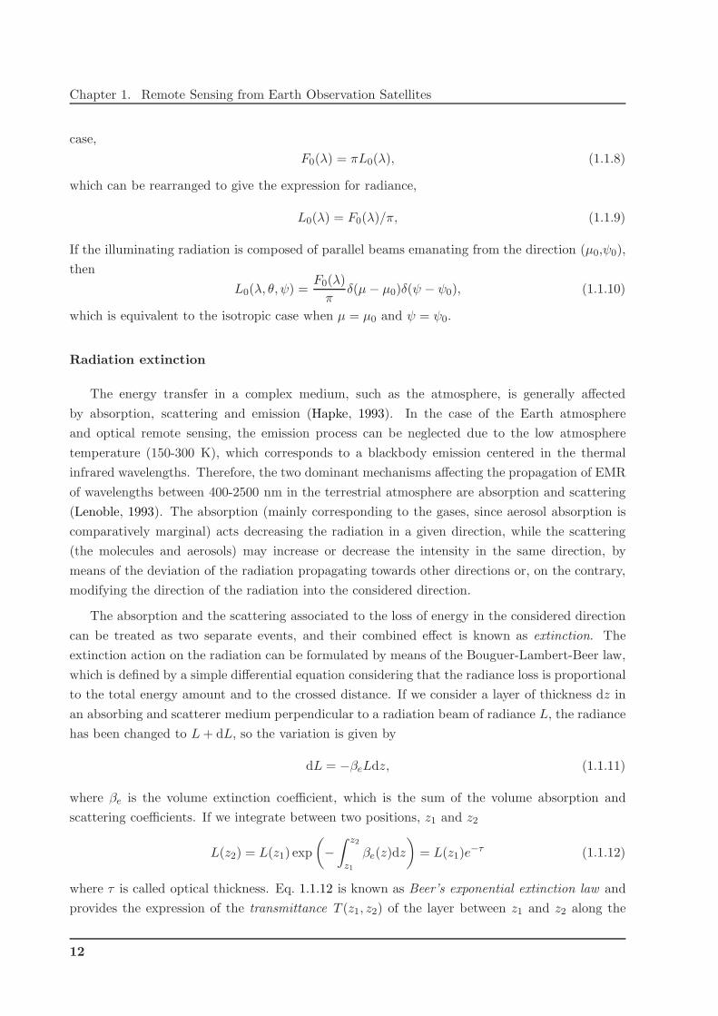
scattering coefficients. If we integrate between two positions, z1 and z2
L(z2) = L(z1) exp
(
−∫ z2
z1
βe(z)dz
)
= L(z1)e−τ (1.1.12)
where τ is called optical thickness. Eq. 1.1.12 is known as Beer’s exponential extinction law and
provides the expression of the transmittance T (z1, z2) of the layer between z1 and z2 along the
12

1.1. Electromagnetic Radiation and Radiative Transfer
direction of propagation by
T (z1, z2) =L(z2)
L(z1)= e−τ . (1.1.13)
The optical thickness (often referred to as optical depth) serves as a measure of the opacity or
turbidity of the atmosphere for a given wavelength of EMR. From an altitude z above the Earth’s
surface to the TOA, the total optical depth is calculated as
τtot(λ) =
∫ ∞
zβe(λ, z)dz =
∫ ∞
zκtot(λ)δatm(z)dz, (1.1.14)
where κtot(λ) is the total extinction coefficient (which can be specified for each of the molecular
species in the atmosphere) and δatm(z) is the density of the intervening atmosphere between z and
the TOA. For the absorbing and scattering atmospheres we have respectively the absorbing and
scattering optical thicknesses τabs(λ) and τdif(λ). The solar intensity measured at the Earth’s sur-
face assumes the form of the extinction Bouguer-Lambert-Beer law, Ls(λ) = L0(λ) exp(−τtot(λ)).
TOA Signal Formulation
A simple but accurate formulation of the TOA signal measured by the space-borne sensor in
terms of surface reflectance and atmospheric optical parameters is necessary for the evaluation
of TOA radiance (Liou, 2002). In this formulation, the TOA radiance is expressed as a sum of
radiative terms from different processes, such as the radiation scattered by the atmosphere into
the sensor line of sight, or the direct radiation multiply scattered between the atmosphere and
the surface.
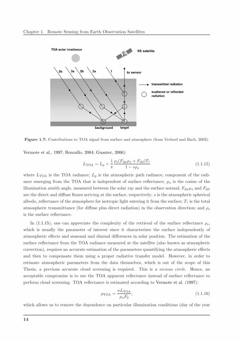
Specifically, the contribution of the target to the upward TOA radiance can be decomposed as
the sum of five terms, which are shown in Fig. 1.7: (1) the photons reflected by the atmosphere
before reaching the surface, (2a) the photons directly transmitted from the Sun to the target and
directly reflected back to the sensor, (2b) the photons scattered by the atmosphere then reflected
by the target and directly transmitted to the sensor, (3a) the photons directly transmitted to the
target but scattered by the atmosphere on their way to the sensor, and, finally, (3b) the photons
having at least two interactions with the atmosphere and one with the target.
In this formulation, the direction of propagation of EMR incident at the TOA or Earth’s
surface from the Sun will be denoted by the illumination zenith and azimuth angle, θs and ψs.
Similarly, the direction of EMR emerging from the Earth’s surface-atmosphere system is denoted
by the viewing zenith and azimuth angle, θv and ψv .
The TOA radiance signal registered by a sensor looking at an homogeneous Lambertian4
surface would be given by the following simplified radiative transfer equation (Tanre et al., 1979;
4In Lambertian surfaces the reflected radiance is isotropous or perfectly diffuse. Thus, the reflected field is the
same for all of the points in the surface, and independent of the view angle.
13
Chapter 1. Remote Sensing from Earth Observation Satellites
Figure 1.7: Contributions to TOA signal from surface and atmosphere (from Verhoef and Bach, 2003).
Vermote et al., 1997; Renzullo, 2004; Guanter, 2006):
LTOA = Lp +1
π
ρs(Fdirµs + Fdif)T↑1 − sρs
(1.1.15)
where LTOA is the TOA radiance; Lp is the atmospheric path radiance, component of the radi-
ance emerging from the TOA that is independent of surface reflectance; µs is the cosine of the
illumination zenith angle, measured between the solar ray and the surface normal; Fdirµs and Fdif
are the direct and diffuse fluxes arriving at the surface, respectively; s is the atmospheric spherical
albedo, reflectance of the atmosphere for isotropic light entering it from the surface; T↑ is the total
atmospheric transmittance (for diffuse plus direct radiation) in the observation direction; and ρs
is the surface reflectance.
In (1.1.15), one can appreciate the complexity of the retrieval of the surface reflectance ρs,
which is usually the parameter of interest since it characterizes the surface independently of
atmospheric effects and seasonal and diurnal differences in solar position. The estimation of the
surface reflectance from the TOA radiance measured at the satellite (also known as atmospheric
correction), requires an accurate estimation of the parameters quantifying the atmospheric effects
and then to compensate them using a proper radiative transfer model. However, in order to
estimate atmospheric parameters from the data themselves, which is out of the scope of this
Thesis, a previous accurate cloud screening is required. This is a vicious circle. Hence, an
acceptable compromise is to use the TOA apparent reflectance instead of surface reflectance to
perform cloud screening. TOA reflectance is estimated according to Vermote et al. (1997):
ρTOA =πLTOA
µsF0, (1.1.16)
which allows us to remove the dependence on particular illumination conditions (day of the year
14
1.2. Multispectral and Hyperspectral Imaging Spectrometers
and angular configuration) and illumination effects due to rough terrain (cosine correction). It is
worth noting that illumination effects are usually higher than the atmospheric effects depending
on the geometric configuration. Think for example in the huge contrast that can be appreciated
on a spherical object illuminated at an angle with a lamp (Gomez-Sanchis et al., 2008d). One
can see that ρTOA becomes the surface reflectance ρs under the following conditions: atmospheric
path radiance Lp = 0; diffuse illumination Fdif = 0; direct illumination equal to the TOA solar
irradiance Fdir = F0; atmospheric spherical albedo s = 0; and total atmospheric transmittance
T↑ = 1. That is, when the Earth’s atmosphere completely disappears.
1.2 Multispectral and Hyperspectral Imaging Spectrometers
As shown in previous sections, materials reflect, absorb, and emit electromagnetic radia-
tion in different ways depending on their molecular composition and shape. Remote sensing
exploits this physical fact and deals with the acquisition of information about a scene at a
short, medium, or long distance. The radiation acquired by a sensor is measured at different
wavelengths, and the resulting spectral signature (or spectrum) is used to identify a given ma-
terial or to retrieve surface biophysical parameters by means of regression and inversion models
(Gomez-Chova et al., 2001; Gomez-Chova, 2002; Camps-Valls et al., 2005, 2006c, 2008b). The
field of spectroscopy deals with the measurement, analysis, and interpretation of such spectra
(Richards and Jia, 1999); and it is worth noting that it can be applied to a broad range of
problems not related to Earth observation, such as industrial applications (Calpe et al., 2003;
Calpe-Maravilla et al., 2004b, 2005, 2006; Vila et al., 2005; Vila-Frances et al., 2005, 2006b) or
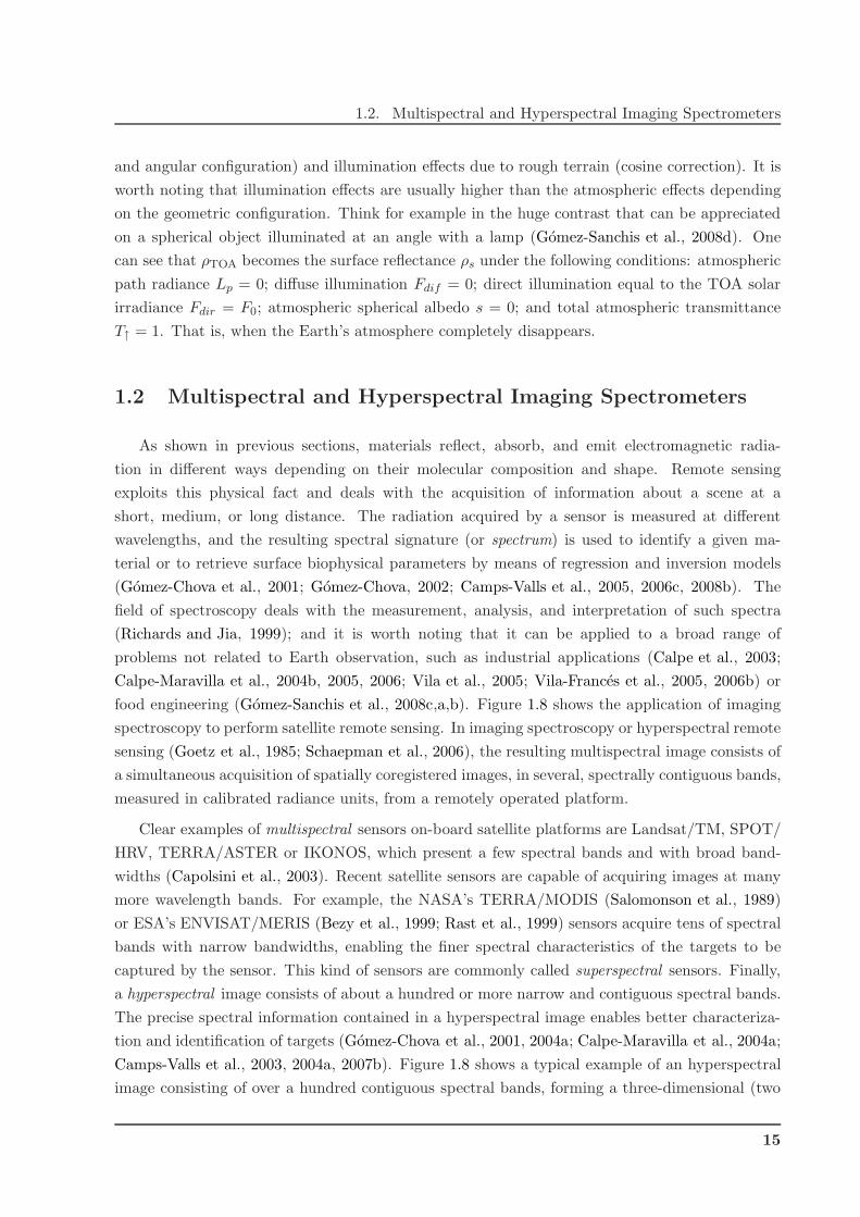
food engineering (Gomez-Sanchis et al., 2008c,a,b). Figure 1.8 shows the application of imaging
spectroscopy to perform satellite remote sensing. In imaging spectroscopy or hyperspectral remote
sensing (Goetz et al., 1985; Schaepman et al., 2006), the resulting multispectral image consists of
a simultaneous acquisition of spatially coregistered images, in several, spectrally contiguous bands,
measured in calibrated radiance units, from a remotely operated platform.
Clear examples of multispectral sensors on-board satellite platforms are Landsat/TM, SPOT/
HRV, TERRA/ASTER or IKONOS, which present a few spectral bands and with broad band-
widths (Capolsini et al., 2003). Recent satellite sensors are capable of acquiring images at many
more wavelength bands. For example, the NASA’s TERRA/MODIS (Salomonson et al., 1989)
or ESA’s ENVISAT/MERIS (Bezy et al., 1999; Rast et al., 1999) sensors acquire tens of spectral
bands with narrow bandwidths, enabling the finer spectral characteristics of the targets to be
captured by the sensor. This kind of sensors are commonly called superspectral sensors. Finally,
a hyperspectral image consists of about a hundred or more narrow and contiguous spectral bands.
The precise spectral information contained in a hyperspectral image enables better characteriza-
tion and identification of targets (Gomez-Chova et al., 2001, 2004a; Calpe-Maravilla et al., 2004a;
Camps-Valls et al., 2003, 2004a, 2007b). Figure 1.8 shows a typical example of an hyperspectral
image consisting of over a hundred contiguous spectral bands, forming a three-dimensional (two
15
Chapter 1. Remote Sensing from Earth Observation Satellites
Figure 1.8: Principle of imaging spectroscopy.
spatial dimensions and one spectral dimension) image cube. Each pixel is associated with a
complete spectrum of the imaged area.
Currently, space-borne hyperspectral imagery is not commercially available. There are only ex-
perimental satellite-sensors that acquire hyperspectral imagery for scientific investigation such as
NASA’s EO1/Hyperion (Ungar et al., 2003) and ESA’s PROBA/CHRIS (Barnsley et al., 2004;
Cutter, 2004b). However, future planned Earth Observation missions (submitted for evalua-
tion and approval) point to a new generation of hyperspectral sensors (Schaepman et al., 2006):
EnMAP (Environmental Mapping and Analysis Program, GFZ/DLR, Germany) (Stuffler et al.,
2007; Kaufmann et al., 2008), FLEX (ESA Earth Explorer proposal) (Stoll et al., 2003; Moreno,
2006), HyspIRI (NASA GSFC proposal) (Green et al., 2008a,b), SpectraSat (Full Spectral Land-
sat proposal), ZASat (South African proposal, University of Stellenbosch), HIS (Chinese Space
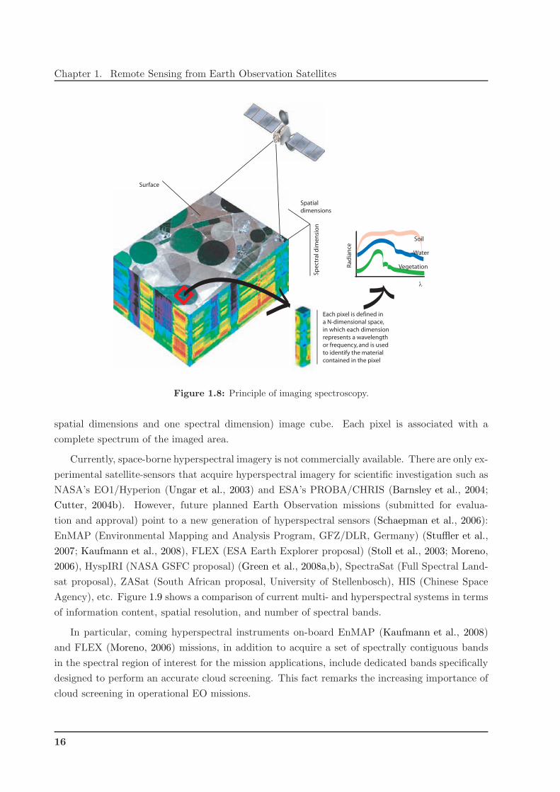
Agency), etc. Figure 1.9 shows a comparison of current multi- and hyperspectral systems in terms
of information content, spatial resolution, and number of spectral bands.
In particular, coming hyperspectral instruments on-board EnMAP (Kaufmann et al., 2008)
and FLEX (Moreno, 2006) missions, in addition to acquire a set of spectrally contiguous bands
in the spectral region of interest for the mission applications, include dedicated bands specifically
designed to perform an accurate cloud screening. This fact remarks the increasing importance of
cloud screening in operational EO missions.
16
1.3. Push-broom Imaging Spectrometers
Multispectral Hyperspectral
Detailed assessments,
monitoring with infrequent
coverage
Large scale assess-
ments, monitoring with
frequent coverage
Figure 1.9: Comparison of multispectral and hyperspectral data and instruments (credits:
http://www.enmap.de/). Left : Comparison of multispectral and hyperspectral measuring data. Right :
Performance comparison of main air- and space-borne multi- and hyperspectral systems in terms of spec-
tral and spatial resolution.
1.3 Push-broom Imaging Spectrometers
Many of the multispectral and hyperspectral sensors are push-broom imaging spectrometers.
Push-broom line imagers consist of an optical system that focalizes the light coming from a portion
of the Earth’s surface onto the focal plane where the sensor is placed. The system includes a long
and narrow slit that limits the area being imaged to a stripe aligned with one of the sensor’s axis,
while a diffractive medium (prism, grid, etc.) forms a spectrum of the line along the orthogonal
axis. Usually, the detector is a charge coupled device (CCD) two-dimensional array whose rows
separate wavelengths and columns separate resolved points in the Earth image (Mouroulis et al.,
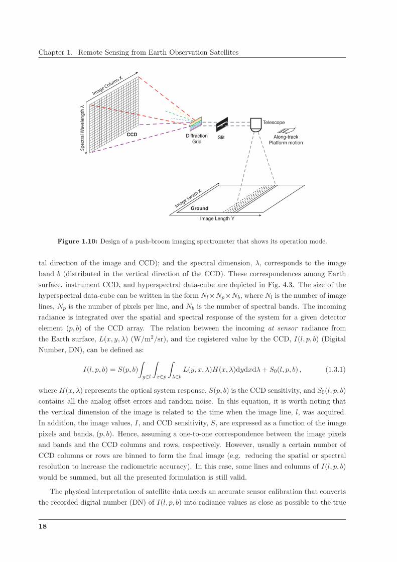
2000). Figure 1.10 shows the push-broom operation mode for the acquisition of spectral images.
The optical system collects the light arriving from a long and narrow strip of the surface below by
means of a thin slit. The slit is oriented perpendicularly to the direction of motion of the sensor,
and the sequential acquisition of lines generates the image as the platform moves forward. The
image of the land strip is spectrally spread out (diffracted for gratings and dispersed for prisms),
separating the different wavelengths, and projected onto a properly aligned CCD array, so the
line is parallel to the horizontal axis (spatial) while the spectral spread out is produced along the
perpendicular axis (spectral).
Therefore, a hyperspectral image consists of two spatial dimensions (along-track and across-
track) and one spectral dimension (wavelength). This hyperspectral image is registered by the
instrument in a data-cube where: the along-track dimension at the Earth surface, y, corresponds
to the image-lines dimension l (distributed in the vertical direction of the image); the surface
across-track dimension, x, corresponds to the line-pixels dimension p (distributed in the horizon-
17
Chapter 1. Remote Sensing from Earth Observation Satellites
CCD
Image Column X
Sp
ec
tra
l Wa
ve
len
gth
λ
Diffraction
GridSlit
Telescope
Along-track
Platform motion
Image Swath
X
Image Length Y
Ground
Figure 1.10: Design of a push-broom imaging spectrometer that shows its operation mode.
tal direction of the image and CCD); and the spectral dimension, λ, corresponds to the image
band b (distributed in the vertical direction of the CCD). These correspondences among Earth
surface, instrument CCD, and hyperspectral data-cube are depicted in Fig. 4.3. The size of the
hyperspectral data-cube can be written in the form Nl×Np×Nb, where Nl is the number of image
lines, Np is the number of pixels per line, and Nb is the number of spectral bands. The incoming
radiance is integrated over the spatial and spectral response of the system for a given detector
element (p, b) of the CCD array. The relation between the incoming at sensor radiance from
the Earth surface, L(x, y, λ) (W/m2/sr), and the registered value by the CCD, I(l, p, b) (Digital
Number, DN), can be defined as:
I(l, p, b) = S(p, b)
∫
y∈l
∫
x∈p
∫
λ∈bL(y, x, λ)H(x, λ)dydxdλ+ S0(l, p, b) , (1.3.1)
where H(x, λ) represents the optical system response, S(p, b) is the CCD sensitivity, and S0(l, p, b)
contains all the analog offset errors and random noise. In this equation, it is worth noting that
the vertical dimension of the image is related to the time when the image line, l, was acquired.
In addition, the image values, I, and CCD sensitivity, S, are expressed as a function of the image
pixels and bands, (p, b). Hence, assuming a one-to-one correspondence between the image pixels
and bands and the CCD columns and rows, respectively. However, usually a certain number of
CCD columns or rows are binned to form the final image (e.g. reducing the spatial or spectral
resolution to increase the radiometric accuracy). In this case, some lines and columns of I(l, p, b)
would be summed, but all the presented formulation is still valid.
The physical interpretation of satellite data needs an accurate sensor calibration that converts
the recorded digital number (DN) of I(l, p, b) into radiance values as close as possible to the true
18
1.3. Push-broom Imaging Spectrometers
radiance L(l, p, b). Most of existing CCD sensors allow an accurate correction of dark current
offsets, thus making S0(l, p, b) negligible (remaining only a zero mean, low amplitude random
noise). Therefore, the calibration procedure consists in finding a set of calibration coefficients to
retrieve the true radiance:
L(l, p, b) = a(p, b)I(l, p, b) , (1.3.2)
where a(p, b) is the calibration coefficient at band b on the pixel p, which depends on the optical
system response, H, and the CCD sensitivity, S.
If the instrument works correctly (Mouroulis et al., 2000), the spatial and the spectral dimen-
sions (orthogonal dimensions of the CCD), are independent and they can be processed separately.
Therefore, the optical system response can be expressed as H(x, λ) = H(x)H(λ), where H(x)
represents the slit response and H(λ) represents the instrument chromatic response, which in
turn defines the wavelength and bandwidth of each band. Thus, the slit response is constant for
all the lines and bands of a given image, and independent from pixel-to-pixel. This is known as
uniformity.
Assuming a smooth optical response, the integral of the incoming radiance over the optical
response of the system in (1.3.1), which represents the radiance at the focal plane array of the
CCD, can be approximated as:∫
y∈l
∫
x∈p
∫
λ∈bL(y, x, λ)H(x)H(λ)dydxdλ = L(l, p, b)Hx(p)Hλ(b) (1.3.3)
where Hx(p) and Hλ(b) represent the contribution of the spatial and spectral response to the
calibration coefficient of the detector element (p, b). Then, the relation between the incoming
radiance and the registered value by the CCD of (1.3.1) can be written as:
I(l, p, b) = L(l, p, b)Hx(p)Hλ(b)S(p, b) + S0(l, p, b) , (1.3.4)
and the different contributions to the ideal calibration coefficients (S0(l, p, b) ≃ 0) would be:
a(p, b) =L(l, p, b)
I(l, p, b)=
1
Hx(p)Hλ(b)S(p, b). (1.3.5)
Summarizing, the complete optical design is optimized so that monochromatic images of the
slit fall on straight CCD rows, and line spectra of resolved ground areas fall on CCD columns. In
this case, each pixel in a line of the image at a given wavelength has been acquired by a different
element of the CCD; while every column of the image for that wavelength has been measured by
the same element of the CCD. Would be the CCD and the slit ideally built then all the CCD
elements would have the same sensitivity and response, producing even and noise-free images.
However, in real devices, deviations from these design conditions produce the following problems:
• Optical aberrations and misalignments in the CCD integration with optics cause the spec-
trometer entrance slit image to be projected as a curve on the detector array. This causes a
bending of spectral lines across the spatial axis and of the spatial lines across the spectral
axis (Goetz et al., 2003).
19
Chapter 1. Remote Sensing from Earth Observation Satellites
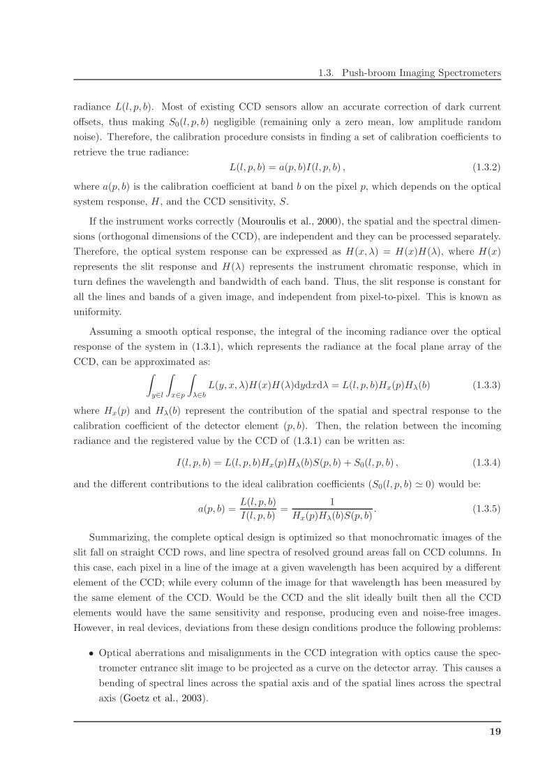
Figure 1.11: ENVISAT/MERIS system. Left : Location of MERIS on ENVISAT. Right : MERIS instru-
ment. (Credits: ESA)
– Deviations of the monochromatic images of the slit from the CCD rows are known
as smile (curved up) or frown (curved down). It causes a non-linear variation in the
wavelength in the across-track direction, which results in a spectral shift from nominal
spectral band positions along the CCD columns.
– Deviations of the line spectra of resolved ground areas from the CCD columns are
known as chromatic keystone. It causes images of the slit at different wavelengths to
differ in length depending on where the ray propagates with respect to the center of
the lens.
• Sensitivity variations between neighboring elements of the CCD and variations on the width
of the slit along its length results in the intensity of an homogeneous area to be slightly
different in each column of the CCD array (Barducci and Pippi, 2001).
– The effect of these imperfections in the resulting image is a vertical pattern known as
vertical striping.
A more detailed description of the sensor calibration and the proposed correction of presented
errors is given in chapter 4 for the imaging spectrometers used in this Thesis.
1.3.1 The MEdium Resolution Imaging Spectrometer (MERIS)
The MEdium Resolution Imaging Spectrometer (MERIS) instrument (Rast et al., 1999) is
mounted on board the ENVIronmental SATellite (ENVISAT) Earth Observation Satellite launched
20
1.3. Push-broom Imaging Spectrometers
400 600 800 10000
0.5
1
wavelength (nm)
MERIS spectral channels
MERISspectral bandsAtmospheric transmissionVegetation spectral signatureBare soil spectral signature
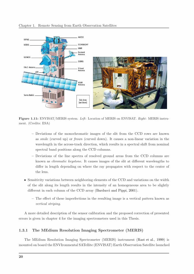
Figure 1.12: MERIS band locations (red) superimposed to a reflectance spectra of healthy vegetation
(green), bare soil (black), and the atmospheric transmittance (blue).
by the European Space Agency in March 2002. MERIS on ENVISAT is a programmable medium
resolution imaging spectrometer operating in the VNIR spectral range (400-900 nm). The EN-
VISAT/MERIS system is depicted in Fig 1.11.
The instrument scans the Earth’s surface in a push-broom mode. The satellite’s motion
provides scanning in the along-track direction, and the scene is imaged simultaneously across
the entire spectral range through a dispersing system onto a CCD array, resulting the spatial
sampling in the across-track direction. MERIS is designed so that it can acquire data over
the Earth whenever illumination conditions are suitable (illumination angles below 80◦) with
high radiometric (1% to 5%) and spectrometric (1 nm) performance. Fifteen spectral bands can
be selected by ground command, each of them has a programmable width and location in the
390 nm to 1040 nm spectral range (Merheim-Kealy et al., 1999). However, a fixed set of bands
was recommended by the Science Advisory Group and frozen before launch. It is presented in
Table 1.1 and depicted in Fig 1.12. The Level 2 ESA products are being developed and will be
validated for this set of bands, although it is possible to use alternative band sets for experimental
campaigns of a few weeks duration.
The MERIS’ 68.5◦ field of view (FOV) around nadir covers a swath width of 1150 km at a
nominal altitude of 800 km. It allows global coverage of the Earth in 3 days. The instantaneous
FOV is divided into five segments, each of them is imaged by one of the corresponding five
cameras.A slight overlap exists between the FOVs of adjacent optical cameras. An area CCD
detector is used, with an instantaneous detector element FOV of 1.149 arcmin.
MERIS provides either full spatial resolution data (FR) or reduced spatial resolution data
(RR). These two spatial resolutions, for the nominal orbit are:
• Full spatial resolution: 260 m across track, 290 m along track. Full FR scenes have
2241×2241 pixels and cover 582 km (swath) by 650 km (azimuth). Quarter scenes have
1153×1153 pixels and cover 300 km (swath) by 334 km (azimuth).
• Reduced spatial resolution: 1040 m across track, 1160 m along track. A reduced spatial
21
Chapter 1. Remote Sensing from Earth Observation Satellites
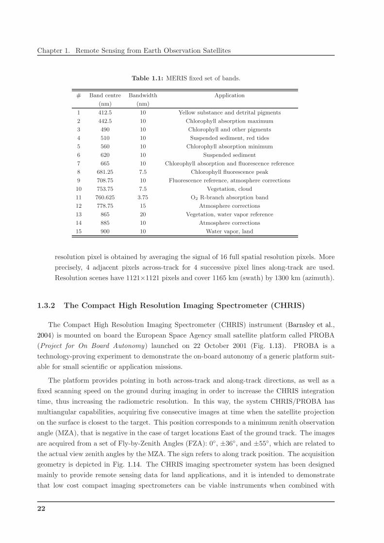
Table 1.1: MERIS fixed set of bands.
# Band centre Bandwidth Application
(nm) (nm)
1 412.5 10 Yellow substance and detrital pigments
2 442.5 10 Chlorophyll absorption maximum
3 490 10 Chlorophyll and other pigments
4 510 10 Suspended sediment, red tides
5 560 10 Chlorophyll absorption minimum
6 620 10 Suspended sediment
7 665 10 Chlorophyll absorption and fluorescence reference
8 681.25 7.5 Chlorophyll fluorescence peak
9 708.75 10 Fluorescence reference, atmosphere corrections
10 753.75 7.5 Vegetation, cloud
11 760.625 3.75 O2 R-branch absorption band
12 778.75 15 Atmosphere corrections
13 865 20 Vegetation, water vapor reference
14 885 10 Atmosphere corrections
15 900 10 Water vapor, land
resolution pixel is obtained by averaging the signal of 16 full spatial resolution pixels. More
precisely, 4 adjacent pixels across-track for 4 successive pixel lines along-track are used.
Resolution scenes have 1121×1121 pixels and cover 1165 km (swath) by 1300 km (azimuth).
1.3.2 The Compact High Resolution Imaging Spectrometer (CHRIS)
The Compact High Resolution Imaging Spectrometer (CHRIS) instrument (Barnsley et al.,
2004) is mounted on board the European Space Agency small satellite platform called PROBA
(Project for On Board Autonomy) launched on 22 October 2001 (Fig. 1.13). PROBA is a
technology-proving experiment to demonstrate the on-board autonomy of a generic platform suit-
able for small scientific or application missions.
The platform provides pointing in both across-track and along-track directions, as well as a
fixed scanning speed on the ground during imaging in order to increase the CHRIS integration
time, thus increasing the radiometric resolution. In this way, the system CHRIS/PROBA has
multiangular capabilities, acquiring five consecutive images at time when the satellite projection
on the surface is closest to the target. This position corresponds to a minimum zenith observation
angle (MZA), that is negative in the case of target locations East of the ground track. The images
are acquired from a set of Fly-by-Zenith Angles (FZA): 0◦, ±36◦, and ±55◦, which are related to
the actual view zenith angles by the MZA. The sign refers to along track position. The acquisition
geometry is depicted in Fig. 1.14. The CHRIS imaging spectrometer system has been designed
mainly to provide remote sensing data for land applications, and it is intended to demonstrate
that low cost compact imaging spectrometers can be viable instruments when combined with
22
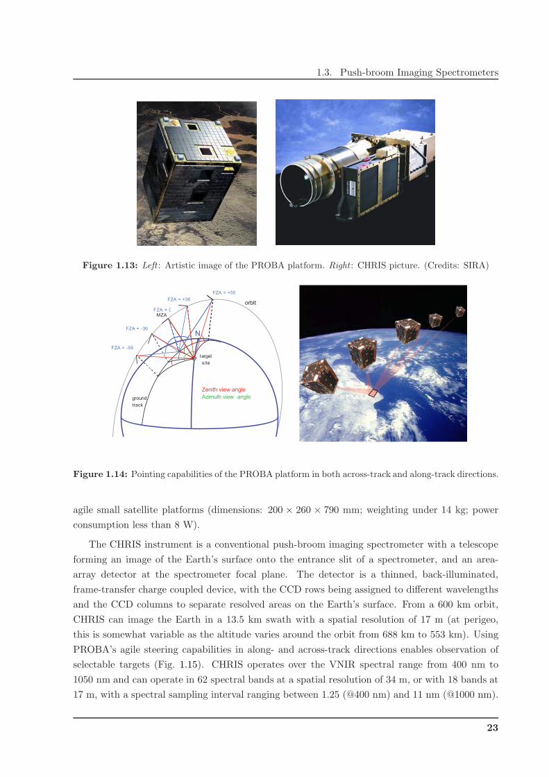
1.3. Push-broom Imaging Spectrometers
Figure 1.13: Left : Artistic image of the PROBA platform. Right : CHRIS picture. (Credits: SIRA)
target
site
N
MZA
orbit
ground
track
FZA = +55
FZA = +36
FZA = 0
FZA = -36
FZA = -55
Zenith view angle
Azimuth view angle
Figure 1.14: Pointing capabilities of the PROBA platform in both across-track and along-track directions.
agile small satellite platforms (dimensions: 200 × 260 × 790 mm; weighting under 14 kg; power
consumption less than 8 W).
The CHRIS instrument is a conventional push-broom imaging spectrometer with a telescope
forming an image of the Earth’s surface onto the entrance slit of a spectrometer, and an area-
array detector at the spectrometer focal plane. The detector is a thinned, back-illuminated,
frame-transfer charge coupled device, with the CCD rows being assigned to different wavelengths
and the CCD columns to separate resolved areas on the Earth’s surface. From a 600 km orbit,
CHRIS can image the Earth in a 13.5 km swath with a spatial resolution of 17 m (at perigeo,
this is somewhat variable as the altitude varies around the orbit from 688 km to 553 km). Using
PROBA’s agile steering capabilities in along- and across-track directions enables observation of
selectable targets (Fig. 1.15). CHRIS operates over the VNIR spectral range from 400 nm to
1050 nm and can operate in 62 spectral bands at a spatial resolution of 34 m, or with 18 bands at
17 m, with a spectral sampling interval ranging between 1.25 (@400 nm) and 11 nm (@1000 nm).
23
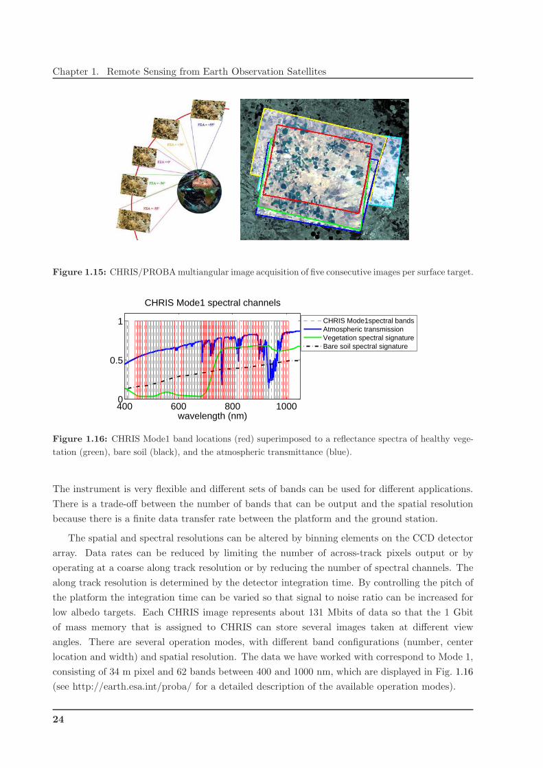
Chapter 1. Remote Sensing from Earth Observation Satellites
Figure 1.15: CHRIS/PROBA multiangular image acquisition of five consecutive images per surface target.
400 600 800 10000
0.5
1
wavelength (nm)
CHRIS Mode1 spectral channels
CHRIS Mode1spectral bandsAtmospheric transmissionVegetation spectral signatureBare soil spectral signature
Figure 1.16: CHRIS Mode1 band locations (red) superimposed to a reflectance spectra of healthy vege-
tation (green), bare soil (black), and the atmospheric transmittance (blue).
The instrument is very flexible and different sets of bands can be used for different applications.
There is a trade-off between the number of bands that can be output and the spatial resolution
because there is a finite data transfer rate between the platform and the ground station.
The spatial and spectral resolutions can be altered by binning elements on the CCD detector
array. Data rates can be reduced by limiting the number of across-track pixels output or by
operating at a coarse along track resolution or by reducing the number of spectral channels. The
along track resolution is determined by the detector integration time. By controlling the pitch of
the platform the integration time can be varied so that signal to noise ratio can be increased for
low albedo targets. Each CHRIS image represents about 131 Mbits of data so that the 1 Gbit
of mass memory that is assigned to CHRIS can store several images taken at different view
angles. There are several operation modes, with different band configurations (number, center
location and width) and spatial resolution. The data we have worked with correspond to Mode 1,
consisting of 34 m pixel and 62 bands between 400 and 1000 nm, which are displayed in Fig. 1.16
(see http://earth.esa.int/proba/ for a detailed description of the available operation modes).
24

1.4. Motivation
1.4 Motivation
This Thesis is intended to support the scientific and technological interest in MERIS and
CHRIS (or other VIS/IR multispectral sensors) data for Earth observation studies. For an accu-
rate exploitation of remote sensing data provided by these sensors, the ideal situation would be
the availability of additional products containing relevant information about cloud characteristics
simultaneous to the image acquisition and with the same spatial resolution. This can be accom-
plished if cloud detection is achieved directly from the data by means of the measured radiances in
some properly selected wavelengths. Therefore, the main objective is to provide new operational
cloud screening tools for the derivation of cloud location and abundance maps, thus allowing the
retrieval of atmospheric and surface biophysical parameters from satellite data taken over land
and ocean.
Several aspects of these sensors justify the approach. Two of the key features of MERIS are
its temporal resolution (revisit time of 3 days) and its spatial coverage (swath width of 1150 km).
In addition, MERIS also provides data at an unprecedented combination of spectral and spatial
resolutions: 15 narrow bands and 300 m pixel size in full resolution (FR) mode. Therefore, MERIS
has a great potential for multitemporal studies both at regional and global scales. The operational
use of MERIS images is, however, hampered by the presence of clouds because this instrument
works in the VNIR part of the electromagnetic spectrum. On this matter, an automatic and
accurate cloud screening method is essential in order to use partially cloudy images facilitating
the elaboration of MERIS products and also improving the usability of MERIS temporal series.
Two major points motivate the selection of MERIS data and cloud screening to be put together
in this Thesis. On the one hand, MERIS offers a unique spectral configuration for the retrieval
of both atmosphere and surface parameters: two fine bands at the oxygen (O2-A) and water
vapor atmospheric absorptions are combined with other thirteen channels providing high-accuracy
measurements from the blue to the near-infrared spectral regions (see Rast et al. (1999) for further
technical information). The accurate characterization of the O2-A absorption at MERIS band
11 enables the estimation of cloud top height from MERIS data (Preusker et al., 2006). On the
other hand, the lack of operative methods for the cloud screening of MERIS data, as well as
identified problems in the corresponding ESA Official Level 2 cloud mask products, are known
(Santer et al., 1999).
The other sensor included in this study is the CHRIS hyperspectral instrument mounted on
board PROBA. Thanks to the PROBA platform pointing capabilities and small CHRIS spatial
coverage (typical image areas about 13 km2), the acquisition plan of CHRIS tries to avoid acqui-
sitions with cloud coverage, but usually images are partially affected by clouds. In these cases,
users that requested the acquisition have a special interest in an accurate cloud screening in order
to identify the cloud-free areas of the scene. In addition, the high spectral and spatial resolution
of CHRIS makes it a good choice in order to propose and validate cloud detection methodologies
for next generation of satellite hyperspectral instruments.
25

Chapter 1. Remote Sensing from Earth Observation Satellites
26
Chapter 2
Cloud Screening from Earth
Observation Images
Clouds can be defined as a mass of condensed water vapor or ice particles suspended above
the Earth’s surface. Accurate identification of clouds in remote sensing images is a key issue
for a wide range of remote sensing applications, especially in the case of sensors working in the
VNIR range of the electromagnetic spectrum due to the severe absorption and scattering of cloud
constituents at these wavelengths. The amount of images acquired over the globe every day
by the instruments on board Earth Observation satellites makes inevitable that many of these
images present cloud covers, whose extent depends on the season and the geographic position of
the study region. According to the observational estimates from the International Satellite Cloud
Climatology Project (ISCCP) data set (Zhang et al., 2004), the global annual-mean cloud cover
is around 66%. Other studies report higher rates of cloud covers over the globe analyzing data
from a worldwide meteorological network with a large number of stations at different latitudes
and seasons (Breon and Colzy, 1999). Figure 2.1 shows the total cloud amount (%) from the
ISCCP-D2 monthly mean dataset for the period July 1983 through June 2005 (products from the
ISCCP-D2 dataset are available and can be generated on-line at http://isccp.giss.nasa.gov).
The presence of clouds drastically affects the measured electromagnetic signal and thus the
retrieved information about the observed target. The corresponding cloud influence depends on
the cloud type, cloud cover, cloud height and cloud distribution in the sky, e.g. thick opaque clouds
impede the incoming radiation reaching the surface, while thin transparent clouds contaminate
the data by photons scattered in the observation direction, or attenuate the signal by the removal
of photons in their travel to the sensor. An important issue here is to stress that, depending on
the remote sensing application, clouds can be either viewed as a source of contamination that
makes the image partly useless for assessing landscape properties, or a source of information for
measuring important climatological parameters (Peixoto and Oort, 1992).
• Without an accurate cloud masking, undetected clouds in the scene are the most significant
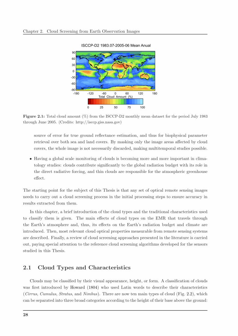
Chapter 2. Cloud Screening from Earth Observation Images
ISCCP-D2 1983.07-2005-06 Mean Anual
90
60
30
0
-30
-60
-90
-180 -120 -60 0 60 120 180
0 25 50 75 100
Total Cloud Amount (%)
Figure 2.1: Total cloud amount (%) from the ISCCP-D2 monthly mean dataset for the period July 1983
through June 2005. (Credits: http://isccp.giss.nasa.gov)
source of error for true ground reflectance estimation, and thus for biophysical parameter
retrieval over both sea and land covers. By masking only the image areas affected by cloud
covers, the whole image is not necessarily discarded, making multitemporal studies possible.
• Having a global scale monitoring of clouds is becoming more and more important in clima-
tology studies: clouds contribute significantly to the global radiation budget with its role in
the direct radiative forcing, and thin clouds are responsible for the atmospheric greenhouse
effect.
The starting point for the subject of this Thesis is that any set of optical remote sensing images
needs to carry out a cloud screening process in the initial processing steps to ensure accuracy in
results extracted from them.
In this chapter, a brief introduction of the cloud types and the traditional characteristics used
to classify them is given. The main effects of cloud types on the EMR that travels through
the Earth’s atmosphere and, thus, its effects on the Earth’s radiation budget and climate are
introduced. Then, most relevant cloud optical properties measurable from remote sensing systems
are described. Finally, a review of cloud screening approaches presented in the literature is carried
out, paying special attention to the reference cloud screening algorithms developed for the sensors
studied in this Thesis.
2.1 Cloud Types and Characteristics
Clouds may be classified by their visual appearance, height, or form. A classification of clouds
was first introduced by Howard (1804) who used Latin words to describe their characteristics
(Cirrus, Cumulus, Stratus, and Nimbus). There are now ten main types of cloud (Fig. 2.2), which
can be separated into three broad categories according to the height of their base above the ground:
28

2.1. Cloud Types and Characteristics
Figure 2.2: Types of cloud according to the height of their base above the ground and their vertical
distribution (Credits: BBC Weather).
high clouds, medium clouds and low clouds (Stephens, 2003). Most of the main cloud types are
often subdivided further on the basis of their shape, structure and degree of transparency:
• High clouds. These are usually composed solely of ice crystals and have a base between 7000
and 18000 m.
– Cirrus - white filaments.
– Cirrocumulus - small rippled elements.
– Cirrostratus - transparent sheet, often with a halo.
• Medium clouds. These are usually composed of water droplets and ice crystals, and have a
base between 2000 and 7000 m.
– Altocumulus. - layered, rippled elements, generally white with some shading.
– Altostratus. - thin layer, grey, allows sun to appear as if through ground glass.
– Nimbostratus. - thick layer, low base, dark, rain or snow may fall from it.
• Low clouds. These are usually composed of water droplets, though cumulonimbus clouds
include ice crystals, and have a base usually below 2000 m.
– Stratocumulus - layered, series of rounded rolls, generally white with some shading.
– Stratus - layered, uniform base, grey.
– Cumulus - individual cells, vertical rolls or towers, flat base.
– Cumulonimbus - large cauliflower-shaped towers, often ’anvil tops’ sometimes giving
thunderstorms, or showers of rain or snow.
29
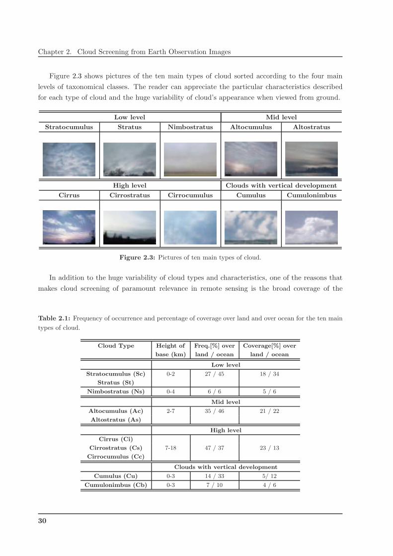
Chapter 2. Cloud Screening from Earth Observation Images
Figure 2.3 shows pictures of the ten main types of cloud sorted according to the four main
levels of taxonomical classes. The reader can appreciate the particular characteristics described
for each type of cloud and the huge variability of cloud’s appearance when viewed from ground.
Low level Mid level
Stratocumulus Stratus Nimbostratus Altocumulus Altostratus
High level Clouds with vertical development
Cirrus Cirrostratus Cirrocumulus Cumulus Cumulonimbus
Figure 2.3: Pictures of ten main types of cloud.
In addition to the huge variability of cloud types and characteristics, one of the reasons that
makes cloud screening of paramount relevance in remote sensing is the broad coverage of the
Table 2.1: Frequency of occurrence and percentage of coverage over land and over ocean for the ten main
types of cloud.
Cloud Type Height of Freq.[%] over Coverage[%] over
base (km) land / ocean land / ocean
Low level
Stratocumulus (Sc) 0-2 27 / 45 18 / 34
Stratus (St)
Nimbostratus (Ns) 0-4 6 / 6 5 / 6
Mid level
Altocumulus (Ac) 2-7 35 / 46 21 / 22
Altostratus (As)
High level
Cirrus (Ci)
Cirrostratus (Cs) 7-18 47 / 37 23 / 13
Cirrocumulus (Cc)
Clouds with vertical development
Cumulus (Cu) 0-3 14 / 33 5/ 12
Cumulonimbus (Cb) 0-3 7 / 10 4 / 6
30

2.2. Clouds and the Energy Cycle
Earth’s surface by clouds when viewed from the space. Clouds cover more than 60% of the
Earth’s surface (Zhang et al., 2004). In particular, average global coverage over the oceans is
about 65% and over the land is about 52%. Table 2.1 provides a frequency of occurrence and
percentage of coverage over land and over ocean depending on the type of cloud.
For the subject of this Thesis, the interest on cloud types comes from the effect of different
clouds on the solar radiation that is used by remote sensing sensors to observe the Earth. Low
and high clouds have different effects on the radiation field with contrary effects on the Earth’s
radiation budget. Whether a given cloud will heat or cool the surface depends on several factors,
including the cloud’s altitude, its size, and the make-up of the particles that form the cloud.
Moreover, cloud detection will not be concerned in identifying cloud type but only presence (and
probability) of clouds.
2.2 Clouds and the Energy Cycle
The Sun’s radiant energy is the fuel that drives Earth’s climate engine. Energy received from
the Sun is mostly in the visible (or shortwave) part of the electromagnetic spectrum. About
30% of the solar energy that comes to Earth is reflected back to space. The ratio of reflected-to-
incoming energy is called albedo1 from the Latin word meaning whiteness. The solar radiation
absorbed by the Earth causes the planet to heat up until it radiates (or emits) as much energy
back into space as it absorbs from the Sun. The Earth’s thermal emitted radiation is mostly in
the infrared (or longwave) part of the spectrum. The top of the clouds is usually colder than
the Earth’s surface. If a cloud is formed in a previously clear sky, the cold cloud top reduces the
longwave emission to space, and energy is trapped beneath the cloud top. The trapped energy
increases the temperature of the Earth’s surface and atmosphere until the longwave emission to
space once again balances the incoming absorbed shortwave radiation. This process is called the
greenhouse effect and, taken by itself, causes a heating of the Earth’s climate.
The balance between incoming and outgoing energy is called the Earth’s radiation budget.
As shown in figure 2.4, the Earth’s atmosphere system constantly tries to maintain a balance
between the energy that reaches the Earth from the Sun and the energy that flows from Earth
back out to space.
The most important components of the Earth’s system to the radiation budget are the planet’s
surface, atmosphere, and clouds. The effect of clouds on the Earth’s radiation balance is measured
as the difference between the clear-sky and total-scene radiation results. This difference is defined
as cloud-radiative forcing (Kiehl, 1992). Mainly, two cloud effects in the radiation budget can be
distinguished (Fig. 2.5):
• Shortwave rays from the sun are scattered in a cloud. Many of the rays return to space.
1Albedo indicates the fraction of the total solar radiation incident to a body that is reflected by it.
31
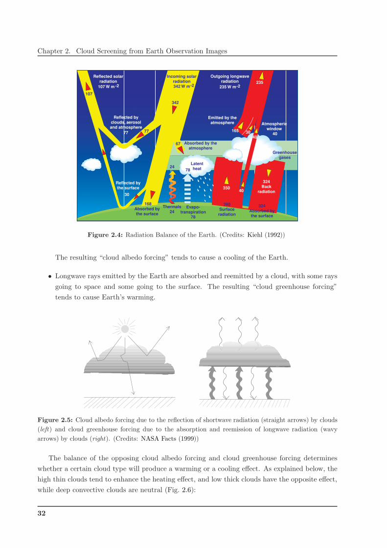
Chapter 2. Cloud Screening from Earth Observation Images
Reflected bythe surface
30
Reflected byclouds, aerosoland atmosphere
77
235
165
-2 -2
Reflected solarradiation
107 W m -2
Outgoing longwaveradiation
235 W m
30
24
67
350
324Back
radiation
324Absorbed bythe surface
Absorbed bythe surface
390Surfaceradiation
40
40
Thermals24
Evapo-transpiration
78
Absorbed by theatmosphere
Emitted by theatmosphere
Greenhousegases
Latentheat
Atmosphericwindow
Incoming solarradiation342 W m
78
40
107
77
342
168
Figure 2.4: Radiation Balance of the Earth. (Credits: Kiehl (1992))
The resulting “cloud albedo forcing” tends to cause a cooling of the Earth.
• Longwave rays emitted by the Earth are absorbed and reemitted by a cloud, with some rays
going to space and some going to the surface. The resulting “cloud greenhouse forcing”
tends to cause Earth’s warming.
Figure 2.5: Cloud albedo forcing due to the reflection of shortwave radiation (straight arrows) by clouds
(left) and cloud greenhouse forcing due to the absorption and reemission of longwave radiation (wavy
arrows) by clouds (right). (Credits: NASA Facts (1999))
The balance of the opposing cloud albedo forcing and cloud greenhouse forcing determines
whether a certain cloud type will produce a warming or a cooling effect. As explained below, the
high thin clouds tend to enhance the heating effect, and low thick clouds have the opposite effect,
while deep convective clouds are neutral (Fig. 2.6):
32

2.3. Cloud Properties
• Low thick clouds reflect more shortwave radiation back to space than the darker surface
would in the absence of the cloud, and thus, less solar energy is available to heat the surface
and atmosphere that tends to cool the Earth’s climate.
• High thin cirrus clouds have a warming effect because they transmit most of the incoming
solar radiation while, simultaneously, they absorb some of the Earth’s infrared radiation
and radiate it back to the surface.
• Deep convective clouds, such as those associated with thunderstorms, have neither a warm-
ing nor a cooling effect because their cloud greenhouse effect, although large, is nearly
balanced by the effect due to the convective clouds’ high albedo.
Figure 2.6: Cloud albedo forcing (straight arrows, which indicate shortwave rays) and cloud greenhouse
forcing (wavy arrows, which indicate longwave rays) of low thick clouds (left), high thin cirrus clouds
(middle), and deep convective clouds (right). (Credit: NASA Facts (1999))
2.3 Cloud Properties
As shown in the previous section, clouds have an important role in energy budget studies due
to its effect on the EMR crossing the Earth’s atmosphere. The cloud cover fraction, cloud type
and the cloud top height have to be known accurately to better quantify the global mean effect of
clouds cooling the climate system and also the effect of clouds on the EMR detected by the remote
sensing sensors. The properties of clouds can vary widely with location, with time of day, with
changing weather, and with season. For these reasons, satellite data play an important role in the
study of clouds as the most effective method to observe clouds on a large scale and to estimate
their impact on the Earth’s climate. The most important cloud optical properties that can be
estimated from remote sensing data are the cloud optical thickness, cloud albedo, and cloud top
pressure:
• Cloud optical thickness: The cloud optical thickness is a measure of the opacity of the cloud.
The cloud optical thickness is an important parameter for the surface and atmospheric
33

Chapter 2. Cloud Screening from Earth Observation Images
energy budget since the variation of cloud optical thickness alters the amount of reflected
radiation and hence the energy that reaches the surface. In addition, the intensity of the
thermal emission from a cloud varies with its temperature and the optical depth or thickness
of the cloud. The optical thickness of a cloud is a measure of not only the physical thickness
of the cloud but also of the amount and phase of water in the cloud. A cloud can be physically
thin, but contain water at a density high enough to produce a high optical thickness. Clouds
that allow most of the sunlight hitting them to pass through them are considered optically
thin. Clouds that reflect most of the sunlight hitting them are considered to be optically
thick. The cloud optical thickness can be determined directly from reflectance data, but its
retrieval depends on the particle size and shape.
• Cloud albedo: The most important cloud parameter for energy budget studies is the cloud
albedo. The cloud albedo is a measurement of the amount of radiation reflected by clouds.
The cloud albedo varies from less than 10 to more that 90 percent of the insolation and
depends on the cloud optical thickness, the size distribution of the cloud droplets, the liquid
water content, the water vapor content, and the Sun’s zenith angle. The smaller the drops
and the greater the liquid water content, the greater the cloud albedo, if all other factors
are the same.
• Cloud top pressure: The cloud top pressure is a measurement of pressure that represents
the location of the radiating top of the clouds (if there is a very tenuous upper portion,
this value may be below where the first cloud particles are found). It can be considered as
equivalent to cloud top height above mean sea level.
By using a simple relationship between the presented cloud optical properties, the ISCCP
has suggested an alternative method of classifying clouds into the traditional cloud types. This
method classifies clouds based upon how optically thick they are and how high they are in the sky.
Figure 2.7 shows how this method classifies clouds based on their optical thickness and cloud top
pressure (cloud top height). The cloud type names represent only an approximate climatological
relationship between the satellite-measured optical parameters and the classical morphological
cloud types. However, a detailed comparison of the satellite and surface-based cloud observations
supports this assignment of names.
The estimation of cloud optical properties involves the use of radiative transfer models and also
an accurate localization of clouds in the image is required. However, it would be advantageous
that the cloud screening algorithm, in addition to detecting clouds accurately, also provided a
cloud abundance index per pixel instead of a binary classification. This added-value information
may be used as follows:
1. To better describe clouds in order to include their properties (abundance, type, height,
subpixel coverage) in radiation models (Tian et al., 1999).
34
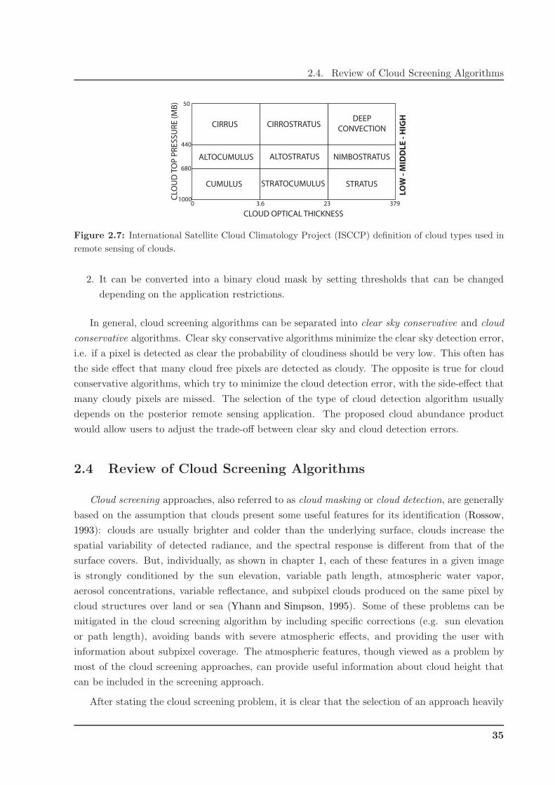
2.4. Review of Cloud Screening Algorithms
CIRROSTRATUS CIRRUS
STRATOCUMULUS
NIMBOSTRATUS
STRATUS
ALTOSTRATUS
DEEP
CONVECTION
ALTOCUMULUS
CUMULUS
CLOUD OPTICAL THICKNESS
CLO
UD
TO
P P
RE
SS
UR
E (
MB
) 50
440
680
10000 3.6 23 379
LO
W -
MID
DL
E -
HIG
H
Figure 2.7: International Satellite Cloud Climatology Project (ISCCP) definition of cloud types used in
remote sensing of clouds.
2. It can be converted into a binary cloud mask by setting thresholds that can be changed
depending on the application restrictions.
In general, cloud screening algorithms can be separated into clear sky conservative and cloud
conservative algorithms. Clear sky conservative algorithms minimize the clear sky detection error,
i.e. if a pixel is detected as clear the probability of cloudiness should be very low. This often has
the side effect that many cloud free pixels are detected as cloudy. The opposite is true for cloud
conservative algorithms, which try to minimize the cloud detection error, with the side-effect that
many cloudy pixels are missed. The selection of the type of cloud detection algorithm usually
depends on the posterior remote sensing application. The proposed cloud abundance product
would allow users to adjust the trade-off between clear sky and cloud detection errors.
2.4 Review of Cloud Screening Algorithms
Cloud screening approaches, also referred to as cloud masking or cloud detection, are generally
based on the assumption that clouds present some useful features for its identification (Rossow,
1993): clouds are usually brighter and colder than the underlying surface, clouds increase the
spatial variability of detected radiance, and the spectral response is different from that of the
surface covers. But, individually, as shown in chapter 1, each of these features in a given image
is strongly conditioned by the sun elevation, variable path length, atmospheric water vapor,
aerosol concentrations, variable reflectance, and subpixel clouds produced on the same pixel by
cloud structures over land or sea (Yhann and Simpson, 1995). Some of these problems can be
mitigated in the cloud screening algorithm by including specific corrections (e.g. sun elevation
or path length), avoiding bands with severe atmospheric effects, and providing the user with
information about subpixel coverage. The atmospheric features, though viewed as a problem by
most of the cloud screening approaches, can provide useful information about cloud height that
can be included in the screening approach.
After stating the cloud screening problem, it is clear that the selection of an approach heavily
35

Chapter 2. Cloud Screening from Earth Observation Images
depends on the characteristics of the instrument. The spectral range, along with the spectral and
spatial resolutions are also critical factors in the selection of the best approach. For example, the
presence of channels in the thermal infrared range enables detection based on thermal contrasts
(Simpson and Gobat, 1996; Papin et al., 2002). Sensors with narrow spectral channels beyond
1 µm have demonstrated good capabilities to detect high clouds because of the strength of the
water vapor absorption (McIntire and Simpson, 2002; Gao et al., 1998). In the spectral range
of 1.38-1.50 µm, both the thin cirrus clouds and the lower-level cumulus clouds can be seen;
however, the surface features are eliminated due to additional absorption of solar radiation by
atmospheric water vapor between clouds and the surface cover (even in presence of ice or snow).
In fact, new generation EO satellites, such as the Global Monitoring for Environment and Security
(GMES) Sentinel 2 and 3 (European Space Agency, 2007), include dedicated bands specifically
designed to perform an accurate cloud screening. These features can not be exploited by recently
developed multispectral sensors that work in the spectral range between 400-1000 nm, such as
CHRIS and MERIS. However, even in these cases, one can take advantage of their high spectral
and radiometric resolution and the specific band locations to increase the cloud detection accuracy,
and to properly describe detected clouds.
In the literature, the simplest approach to mask clouds in a particular scene is the use of a
set of static thresholds (e.g. over features such as albedo or temperature) applied to every pixel
in the image and ultimately providing a binary flag (Wang and Shi, 2006). These methods can
fail for several reasons, such as subpixel clouds, high reflectance surfaces, illumination and obser-
vation geometry, sensor calibration, variation of the spectral response of clouds with cloud type
and height, etc. (Simpson et al., 1998). Spatial coherence methods have an advantage over static
threshold methods because they use the local spatial structure to determine cloud free and cloud
covered pixels. Usually, these algorithms are based on extracted textural features (Tian et al.,
1999; Christodoulou et al., 2003), contextual approaches (Papin et al., 2002), or simple thresholds
applied to the spatial variability of spectral bands (Martins et al., 2002), which is mainly appli-
cable over the ocean where the surface background is sufficiently homogeneous. However, spatial
coherence methods can fail when the cloud system is multi-layered (which is often the case), the
clouds over the scene are smaller than the instrument spatial resolution, or the scene presents
cirrus clouds (which are not opaque). As a consequence, researchers have turned to develop-
ing adaptive threshold cloud-masking algorithms (Simpson et al., 1998; Di Vittorio and Emery,
2002; Yang et al., 2007). Some other algorithms take advantage of the multi-angular (Yang et al.,
2007; Mazzoni et al., 2007) or the multi-temporal (Saitwal et al., 2003) information depending on
the instrument characteristics and the application constraints. In this context, few works using
more sophisticated machine learning tools have been presented so far, such as Bayesian methods
(Murtagh et al., 2003; Li et al., 2003; Merchant et al., 2005), fuzzy logic (Ghosh et al., 2006), arti-
ficial neural networks (Yhann and Simpson, 1995; Tian et al., 1999; McIntire and Simpson, 2002;
Torres Arriaza et al., 2003), or recently kernel methods (Srivastava and Stroeve, 2003; Lee et al.,
2004; Mazzoni et al., 2007).
36

2.4. Review of Cloud Screening Algorithms
Given the extreme complexity of cloud screening, most of the operational cloud masking appli-
cations of current satellite multispectral systems, such as Moderate Resolution Imaging Spectrora-
diometer (MODIS) (Ackerman et al., 1998; Platnick et al., 2003), Advanced Very High Resolution
Radiometer (AVHRR) (Saunders and Kriebel, 1988), Along Track Scanning Radiometer (ATSR)
(Simpson et al., 1998), POLarization and Directionality of the Earth’s Reflectances (POLDER)
(Buriez et al., 1997), or MERIS (Santer et al., 1997), consist in a series of cloud detection thresh-
old tests, which can vary depending on surface type, solar illumination, geographic location, or
climatological criteria.
2.4.1 Reference Cloud Screening Algorithms
The choice of the cloud screening approach is conditioned by the instrument characteristics.
CHRIS and MERIS are optical sensors working in the VNIR range of the spectrum. Two major
points motivate the selection of these instruments and cloud screening to be put together in this
work.
In the case of MERIS, it offers a unique spectral configuration for the retrieval of both atmo-
sphere (Guanter et al., 2008a) and surface (Guanter et al., 2007) parameters: two fine bands at
the oxygen (O2-A) and water vapor atmospheric absorptions are combined with thirteen other
spectral bands providing high-accuracy measurements from the blue to the near-infrared spectral
regions (see Rast et al. (1999) for further technical information). Also, the accurate characteri-
zation of the O2-A absorption at MERIS channel 11 enables the estimation of cloud-top pressure
(which is related to cloud height) from MERIS data (Santer et al., 1999; Naud et al., 2003). How-
ever, there is a well-known lack of accurate methods for the cloud screening of MERIS data, as
well as clearly identified problems in the corresponding ESA official Level 2 cloud mask products
(Ramon et al., 2003; MERIS Quality Working Group, 2006).
In the case of CHRIS, it covers a spectral range from 400 nm to 1050 nm with a high number
of spectral bands (up to 62 spectral channels) and with a high spatial resolution (17 or 34 m at
nadir) depending on the acquisition mode. Owing to the PROBA platform pointing capabilities,
the acquisition plan tries to avoid acquisitions with cloud coverage, but occasionally images are
partially affected by clouds. However, since PROBA is an experimental mission, official Level 2
algorithms and products have not been developed and a cloud mask is not provided with CHRIS
products.
Summarizing, as far as author’s knowledge, no cloud screening algorithm have been proposed
in the literature for CHRIS instrument. In the case of MERIS, in addition to the ESA official
Level 2 cloud mask products, several approaches have been proposed in the literature in order to
mitigate identified problems in the standard ESA product (Ranera et al., 2005; Preusker et al.,
2006; Guanter et al., 2008a). In the following, the MERIS Level 2 Cloud Masking (the official
ESA product) and the Cloud Probability Processor (made available to the user community in the
BEAM software) are described in detail.
37

Chapter 2. Cloud Screening from Earth Observation Images
MERIS Level 2 Cloud Masking
MERIS Level 2 products (European Space Agency, 2006) are obtained by further processing
MERIS TOA radiance. In order to take into account the effect of clouds, image pixels clear
enough to pursue atmospheric corrections are first identified as ‘clear sky’ or ‘cloud free’. The
classification process uses the a priori knowledge of a land/ocean map indexed by longitude and
latitude, and the information in the TOA radiance bands to classify each valid pixel into four pixel
classes: ‘clear sky’ or ‘bright pixel’ over both ‘ocean’ or ‘land’. In this classification, bright pixels
include clouds, bright sand or soil, ice, snow, sunglint, etc. Then there is also a need, for bright
pixels, to separate clouds from bright land and ocean surfaces. The proposed pixel identification
algorithm is based on a succession of tests on reflectance in the MERIS bands:
• For pixels identified as land, identification of homogeneous clouds is based on (i) tests on the
ratio of Rayleigh-corrected reflectance at several wavelengths; and (ii) the apparent pressure
estimated in the O2 absorption by two independent methods (a polynomial regression and
an artificial neural network).
• Over ocean, apparent pressure is used to discriminate between cloud and ice or sun glint.
In this case, thresholds are defined as a function of geometrical conditions due to the strong
effects of clouds on the scattering of radiation.
In addition to this classification, some flags are also defined for the possible occurrence of cirrus
clouds or finite clouds. Since the final L2 cloud classification is a hard classification (i.e. no infor-
mation about cloud transparency/contamination is given), these flags are proposed as a warning
for the quality of the atmospheric corrections. Over ocean, a first flag is set from correlations
between apparent pressure in O2 channels and reflectances at 865 nm with a threshold in pressure
corresponding to a too high contribution of the cirrus reflectance. A similar flag is implemented
for land observations.
All these flags (bright pixel, low pressures, pressure confidences, and reflectance ratios) are
finally used to index a decision table which provides the Cloud-Free flag. Pixels flagged as cloudy
are further processed in order to retrieve the cloud albedo, the cloud optical thickness, and the
cloud top pressure. Finally, a simple classification table indexed by the cloud optical thickness
and cloud top pressure is used to provide a cloud type index.
BEAM Cloud Probability Processor
As aforementioned, ESA official Level 2 cloud mask products have shown clearly identified
problems when considering critical cloud screening issues such as cloud borders and bright surfaces
(Ramon et al., 2003; MERIS Quality Working Group, 2006). In consequence, recent alternative
algorithms have been proposed (Ranera et al., 2005; Preusker et al., 2006).
38

2.4. Review of Cloud Screening Algorithms
The Basic ERS & ENVISAT (A)ATSR and MERIS (BEAM) Toolbox is a collection of ex-
ecutable tools (Fomferra and Brockmann, 2005) that was originally developed by ESA to facilitate
the utilization, viewing, and processing of ESA MERIS, (A)ATSR and others (http://envisat.esa.int
/resources/softwaretools/ or http://www.brockmann-consult.de/beam/).
This software includes the BEAM Cloud Probability Processor, which uses a clear sky conservative
cloud detection algorithm which is based on artificial neural networks (Preusker et al., 2006).
The cloud probability algorithm uses nine spectral bands of MERIS, the ratio of band 11 and
10, which is an indication of the absorption due to oxygen, the ECMWF2 surface pressure and
the exact wavelength of band 11 as input. As an output, it yields a probability value ∈ [0, 1]
indicating if a pixel can be regarded as a cloud or not. Such a probability permits a more flexible
way to work with identified clouds compared to a binary cloud mask.
The algorithm uses two different artificial neural nets for prediction purposes. The first one is
used over the open ocean and the second one over land. The distinction between ocean and land
is done using the altitude information. If the altitude is lower than -50 m the ocean net is used.
During development of the algorithm, the Matrix Operator Model (MOMO), a radiative trans-
fer model (Fischer and Grassl, 1991) based on the Matrix Operator Method, was used to simulate
cloud and non-cloud TOA radiance and an artificial neural net was trained. The output of the
neural net is finally scaled into a probability value. The final cloud classification indicates pixels
that are cloudy (probability > 80%), cloud free (probability < 20%) or where it is uncertain
(20% < probability < 80%).
This algorithm provides a more accurate cloud mask than the MERIS Level 2 Cloud Masking
algorithm, but it still misclassifies bright surfaces such as ice and snow covers. Moreover, the cloud
probability provided by the artificial neural net, which may be useful for the users to decide what
is a cloud depending on the application requirements or image conditions, is usually unevenly
distributed around zero and one, and thus, the information provided is equivalent to a binary
cloud mask.
2European Centre for Medium-Range Weather Forecasts: http://www.ecmwf.int/.
39

Chapter 2. Cloud Screening from Earth Observation Images
40

Part II
Methodology for Cloud Identification

Chapter 3
Proposed Methodology for Cloud
Screening
The main objective of this PhD Thesis is to develop an accurate cloud screening algorithm
using the full spectral information provided by MERIS and by CHRIS imaging spectrometers.
The proposed cloud screening algorithm takes advantage of the high spectral and radiometric
resolutions of MERIS, or the high number of spectral bands of CHRIS, and the specific location
of some bands to increase the cloud detection accuracy, such as the oxygen and water vapor
absorption bands. This chapter summarizes the proposed cloud screening procedure and briefly
introduces the different modules that constitute it. Chapters 4, 5, and 6 will be devoted to analyze
in greater detail these parts.
The method should be capable of: (i) detecting clouds accurately; and (ii) providing probabil-
ity or cloud abundance rather than merely cloud flags. The cloud abundance product provided is
not directly related to the retrieval of cloud optical properties (Kokhanovsky et al., 2007b), such
as the cloud optical thickness, which usually relies on radiative transfer models. This added value
product allows the user to apply an adjustable cloud mask depending on the further processing
stages and final use of the image. For example, undetected cloudy pixels heavily affect biophysical
parameter retrieval methods based on the evaluation of the measurements in the shortest wave-
lengths, such as aerosol retrieval, or estimation of water pigments or suspended matter, as well as
to methods relying on temporal composites (Saitwal et al., 2003; Ranera et al., 2005; Plummer,
2005). Slight over-masking of potential cloudy pixels –conservative cloud masking– would be
preferred to guarantee a minimum admissible quality of the final product (Guanter et al., 2008a;
Kaufman et al., 2005; Martins et al., 2002), while other applications such as land use classification
are less sensitive to thin clouds, and thus the associated areas should not be necessarily discarded
(Gomez-Chova et al., 2006f, 2007c; Camps-Valls et al., 2008a). As a result, the method should
be scalable and allow different levels of masking. Hence, a probabilistic mask indicating the cloud
contamination is proposed.
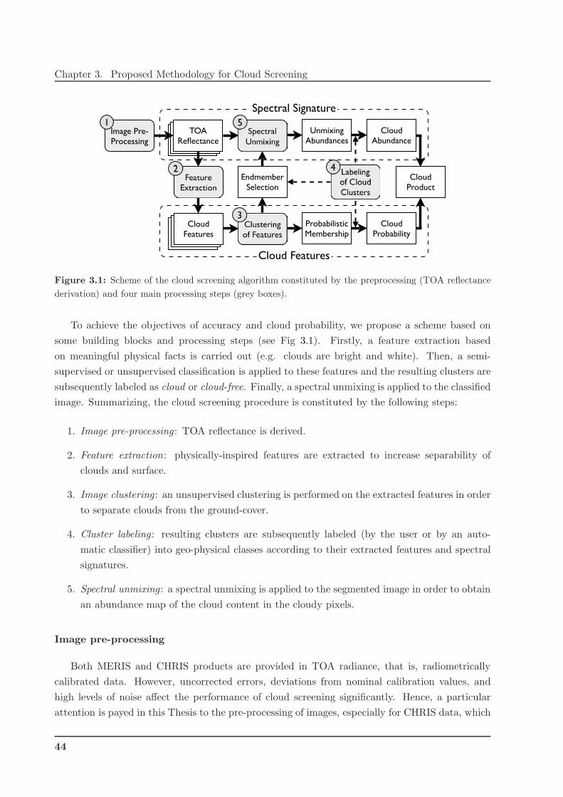
Chapter 3. Proposed Methodology for Cloud Screening
TOA Reflectance
CloudFeatures
Feature Extraction
SpectralUnmixing
UnmixingAbundances
Clustering of Features
EndmemberSelection
Probabilistic Membership
Labelingof Cloud Clusters
CloudAbundance
CloudProbability
CloudProduct
Spectral Signature
Cloud Features
2
3
4
5Image Pre-Processing
1
Figure 3.1: Scheme of the cloud screening algorithm constituted by the preprocessing (TOA reflectance
derivation) and four main processing steps (grey boxes).
To achieve the objectives of accuracy and cloud probability, we propose a scheme based on
some building blocks and processing steps (see Fig 3.1). Firstly, a feature extraction based
on meaningful physical facts is carried out (e.g. clouds are bright and white). Then, a semi-
supervised or unsupervised classification is applied to these features and the resulting clusters are
subsequently labeled as cloud or cloud-free. Finally, a spectral unmixing is applied to the classified
image. Summarizing, the cloud screening procedure is constituted by the following steps:
1. Image pre-processing : TOA reflectance is derived.
2. Feature extraction: physically-inspired features are extracted to increase separability of
clouds and surface.
3. Image clustering : an unsupervised clustering is performed on the extracted features in order
to separate clouds from the ground-cover.
4. Cluster labeling : resulting clusters are subsequently labeled (by the user or by an auto-
matic classifier) into geo-physical classes according to their extracted features and spectral
signatures.
5. Spectral unmixing : a spectral unmixing is applied to the segmented image in order to obtain
an abundance map of the cloud content in the cloudy pixels.
Image pre-processing
Both MERIS and CHRIS products are provided in TOA radiance, that is, radiometrically
calibrated data. However, uncorrected errors, deviations from nominal calibration values, and
high levels of noise affect the performance of cloud screening significantly. Hence, a particular
attention is payed in this Thesis to the pre-processing of images, especially for CHRIS data, which
44

present high levels of noise. In addition, the method must work under many situations. Therefore,
TOA reflectance is estimated to remove the dependence on particular illumination conditions (day
of the year and angular configuration).
Feature Extraction
The measured spectral signature depends on the illumination, the atmosphere, and the sur-
face. Spectral bands free from atmospheric absorptions contain information about the surface
reflectance, while others are mainly affected by the atmosphere. Physically-inspired features that
increase separability of clouds and surface covers can be extracted independently from the bands
that are free from atmospheric effects and from the bands affected by the atmosphere.
With regard the reflectance of the surface, one of the main characteristics of clouds is that
they present bright and white spectra:
• A bright spectrum means that the intensity of the spectral curve (related to the albedo)
should present high values. Therefore, cloud brightness is calculated as the integral of the
spectrum.
• A white spectrum means that the spectral curve is flat, and thus, the first derivative of the
spectral curve should present low values.
Concerning the atmospheric absorptions present in the spectrum of a pixel, another meaningful
feature is the fact that clouds are at a higher altitude than the surface. It is worth noting that
atmospheric absorption depends on the atmospheric components and the optical path. Since light
reflected on high clouds crosses a shorter section of the atmosphere, the consequence would be an
abnormally short optical path, thus weaker atmospheric absorption features. Atmospheric oxygen
or water vapor absorptions (at 760 nm and 940 nm respectively) can be used to estimate this
optical path.
This approach tries to overcome one of the critical issues in cloud detection: the presence
of bright pixels, such as ice/snow in the surface. Bright land covers and clouds have a similar
reflectance behavior, but the atmospheric absorption suffered by cloud pixels is lower than for the
surface pixels due to their height.
Image Clustering and Labeling
At this step, two different approaches have been proposed and analyzed: a fully unsupervised
method and a semi-supervised approach:
1. Unsupervised classification algorithm. In this approach, we use the Expectation-Maximization
(EM) algorithm (Dempster et al., 1977) to estimate the parameters of a Gaussian mixture
45
Chapter 3. Proposed Methodology for Cloud Screening
model (GMM) since it considers the full relationship among variables and provides probabil-
ity maps for each cluster. At this point of the process, the obtained clusters can be labeled
into geo-physical classes taking into account three complementary sources of information:
the thematic map with the distribution of the clusters in the scene, the spectral signatures
of the cluster, and their distribution in the image. Once all clusters have been related to a
class with a geo-physical meaning, it is straightforward to merge all the clusters belonging
to a cloud type. Since the EM algorithm provides posterior probabilities, a probabilistic
cloud index, based on the clustering of the extracted features, can be computed as the sum
of the posteriors of the cloud-clusters. However, if the clusters are well separated in the fea-
ture space, the posteriors decrease drastically from one to zero in the boundaries between
clusters. Therefore, this cloud probability index indicates the probability that one pixel
belongs to a cloud-cluster more likely than to one of the other clusters found in the image,
but it does not give information about the cloud content at a subpixel level, which in turn
becomes very important when dealing with thin clouds or partially covered pixels.
2. Semi-supervised classification algorithm. In this second approach, we develop a semi-
supervised kernel-based method that incorporates labeled and unlabeled data in a general-
purpose learner. The problem of learning from labeled and unlabeled data (semi-supervised
learning) has attracted considerable attention in recent years (Joachims, 2003; Chapelle et al.,
2006). In particular, we focus on two semi-supervised extensions of support vector machines
(SVM) (Scholkopf and Smola, 2001; Shawe-Taylor and Cristianini, 2004; Camps-Valls et al.,
2007c): the so called Laplacian SVM (LapSVM), which introduces an additional regulariza-
tion term on the geometry of both labeled and unlabeled samples by using the graph Lapla-
cian (Belkin et al., 2006; Gomez-Chova et al., 2007b, 2008c); and a novel generative semi-
supervised method based on composite kernels and mean kernel theory (Camps-Valls et al.,
2006d, 2008a; Gomez-Chova et al., 2008a, 2009).
Spectral Unmixing
In order to obtain a cloud abundance map for every pixel in the image, rather than flags
or a binary classification, a spectral unmixing algorithm is applied to the image using the full
spectral information (Chang, 2003). The computed abundances are related to a cluster with a
geo-physical meaning, and the abundance of cloud is computed as the sum of the abundances
of the cloud-clusters. An improved cloud abundance map can be obtained when combining the
cloud abundance and the cloud probability by means of a pixel-by-pixel multiplication. That is,
combining two complementary sources of information processed by independent methods: the
degree of cloud abundance or mixing (obtained from the spectra) and the cloud probability that
is close to one in the cloud-like pixels and close to zero in remaining areas (obtained from the
extracted features). As a result, the proposed algorithm should provide a probabilistic map of
cloud abundance rather than a binary cloud presence flag at a pixel level.
46

Chapter 4
Image Pre-processing and Feature
Extraction
When working with remote sensing images at different times and locations, a desirable charac-
teristic is to have data independent of the sensor system and image acquisition conditions. This is
also true for cloud screening. On the one hand, correcting image data for uncertainties in sensor
calibration has the advantage that then these data are independent of differences in sensor sys-
tem conditions. On the other hand, converting TOA radiance data into TOA reflectance has the
advantage that then these data are corrected for seasonal and diurnal differences in solar position.
Once the image data are expressed in TOA reflectance, we can further process the reflectance
spectra in order to extract features that increase the separability of clouds and surface covers.
These features are physically-inspired and their meaning is independent of differences in the
number, location, and bandwidth of the sensor channels, which is a desirable characteristic for a
cloud screening algorithm intended to work in images acquired by multi and hyperspectral sensors,
such as MERIS and CHRIS.
4.1 Pre-processing (I): TOA Radiance Corrections
Earth observation images acquired by remote sensing instruments are generally affected by two
kinds of noise. The first one can be defined as standard random noise (Aiazzi et al., 2002), which
varies with time and determines the minimum image signal-to-noise ratio (SNR). In addition,
hyperspectral images can present non-periodic partially deterministic disturbance patterns, which
come from the image formation process and are characterized by a high degree of spatial and
spectral coherence (Barducci et al., 2005).
Usually, the whole system is fully characterized after assembly, obtaining the actual gain
correction factors that would produce an even image in operational situations. However, in some
occasions, especially after launch, the system is affected in such a way that the characterization

Chapter 4. Image Pre-processing and Feature Extraction
does not remove completely the noise. In addition, this type of sensors degrade with time, and thus
require a recalibration, which is not always possible. In those cases, a noise reduction algorithm
must be applied after image reception in the pre-processing phase.
In this first section of the chapter, we focus on presenting, modeling, and correcting the
coherent spatial and spectral noise patterns produced by these systematic, yet hardly predictable,
disturbances in both the operational MERIS and the experimental CHRIS instruments.
4.1.1 Corrections for MERIS
ENVISAT is the most important EO satellite ever launched by ESA. The calibration and vali-
dation activities of all ENVISAT instruments represent a long-term effort, which has been carried
out by ESA in parallel to the algorithms improvement (Baudin et al., 1996; Merheim-Kealy et al.,
1999; Delwart et al., 2004).
Calibration involves both pre-launch and post-launch measurements to fully characterize the
payload instruments, and subsequent activities to configure the ground processors to provide
calibrated (Level-1b) data products. MERIS Level 1b (L1b) products are provided in top of
the atmosphere radiance and two different calibration approaches are used to radiometrically
calibrate the data. The primary calibration is the in-flight calibration and characterization of
the instrument that uses the onboard sunlit calibration diffuser plates (Dubuisson et al., 2003;
Ramon et al., 2003; Delwart et al., 2007). Validation of TOA radiances measured by MERIS
are also achieved by comparison with TOA radiance values determined through a number of vi-
carious calibration independent methods: simultaneous in-situ measurements of natural targets
(Hagolle and Cabot, 2004); analysis of Rayleigh scattering over clear water (Martiny et al., 2005);
simulation of radiance data with radiative transfer models (Antoine and Chami, 2004); data ac-
quisition over stable deserts sites (Govaerts and Clerici, 2004); or simultaneous acquisition by
other sensors (Acarreta and Stammes, 2005; Kokhanovsky et al., 2007c).
The scene is acquired simultaneously across the entire spectral range, through a dispersing
system, onto the CCD array (cf. section 1.3). Signals read out from the CCD pass through
several processing steps in order to achieve the required image quality. These CCD processing
tasks include dumping of spectral information from unwanted bands, and spectral integration
to obtain the required bandwidth. Onboard analog electronics perform pre-amplification of the
signal and correlated double sampling and gain adjustment before digitization. The onboard
digital electronics system has three major functions: it completes the spectral integration, it
performs offset and gain corrections in full processed mode, and it creates the reduced-resolution
data when required.
The calibration of MERIS is performed at the orbital south pole, where the calibration diffuser
is illuminated by the Sun by rotating a calibration mechanism. In particular, onboard spectral
calibration is based on the use of absorption bands (Delwart et al., 2007): pink panel that is an
48

4.1. Pre-processing (I): TOA Radiance Corrections
Erbium doped panel with well-defined absorption peaks; the Fraunhoffer lines; and the oxygen
bands. In the calibration mode, correction parameters such as offset and gain are generated,
which are then used to correct the recorded spectra. This correction can be carried out either
on-board or on the ground segment.
A spectral characterization was performed before MERIS launch, which showed a spectral shift
mainly due to the CCD integration with optics during the spatial registration. The so-called smile
effect has a maximum spectral dispersion of 1.5 nm and can be observed at any wavelength. In
fact, MERIS smile is the sole acquisition error that is not corrected in the provided images and has
an important effect in the proposed cloud screening algorithm. However, MERIS smile has been
well characterized in previous works with both in-flight (Dubuisson et al., 2003) and vicarious
(Martiny et al., 2005) calibration methods. This accurate characterization of the spectral shift
produced by the smile can be introduced in the formulation of the cloud screening algorithm in
order to compensate its effects as it will be explained later.
4.1.2 Corrections for CHRIS
PROBA was designed as a technology demonstrator satellite and, originally, CHRIS data
was a secondary objective of the mission. ESA has renewed its support to the PROBA/CHRIS
acquisition plan year by year thanks to the interest of the scientific community, but originally
CHRIS data were not available in the ESA catalogues, and even nowadays CHRIS has no standard
processing algorithms defined. In fact, the only pre-processing step performed to the CHRIS data
before delivering image products is the radiometric calibration1. Thus, CHRIS images present
a certain number of problems and errors that are commonly removed from most of the remote
sensing data.
As a push-broom sensor, the radiometric response of the CHRIS instrument is determined by
two overlapping components: the optical system response (a telescope forming an image onto the
entrance slit together with the spectrometer) and the CCD response (a thinned, back-illuminated,
frame-transfer CCD) (Bernaerts et al., 2000). With regard to the CCD response, the different
pixel-to-pixel response comes from non-uniformities on dark current generation, non-uniformities
on pixel sensitivity, threshold variations, and gain and off-set differences (Theuwissen, 1995). But,
in practice, these CCD imperfections are relatively stable with temperature and time (Cutter,
2004a) resulting in a spatially fixed-pattern noise in the image that should be removed, e.g. the
dark signal offsets are removed by subtracting a generic dark image. However, with regard to
the optical system response, changes in temperature, due to the seasonal variation of the in-orbit
CHRIS instrument temperature (Cutter, 2004a), produce a dilation of the slit and change its
width and moves the image of the slit across the detector. Therefore, the effect of the slit adds up
1CHRIS products are provided in top of the atmosphere radiance in a HDF v4 file format, which includes
additional acquisition information (image date, azimuth and zenith angles, etc) contained in the metadata attributes
of the CHRIS HDF file (Cutter and Johns, 2005b).
49
Chapter 4. Image Pre-processing and Feature Extraction
to the vertical pattern in a complex way, as it is dependent on the sensors temperature heavily
(see Fig. 4.1), and thus it must be modeled and corrected.
Several vertical stripping (VS) reduction approaches have been proposed in the literature. Our
approach falls in the field of the scene-based non-uniformity corrections (SNUCs), since it provides
relative calibration factors directly computed from the acquired image. Methods based on large
uniform areas in the scene or methods assuming constant-static noise patterns (Torres et al.,
2003; Pezoa et al., 2006) are not appropriate for CHRIS due its spatial resolution (17 to 34 m)
and its noise dependence on the sensor’s temperature, respectively. Other methods assume that
all sensor elements observe similar subscenes in a given image and adjust the distributions of
values acquired by each sensor to some reference distribution by means of histogram or moment
matching (Gadallah et al., 2000), but also the high CHRIS spatial resolution and the moderate
number of lines per image dissuade us from its use. Finally, most related methods assume that
noise contribution changes from one pixel to another (high spatial frequency) in the across-track
direction while surface contribution presents smoother profiles (lower spatial frequencies) in the
across-track dimension (Barducci and Pippi, 2001; Garcia and Moreno, 2004; Settle and Cutter,
2005; Mlsna and Becker, 2006). This approach is described in more detail in section 4.1.2 but
the reader is referred to Leathers et al. (2005) for a full description of SNUC methods for push-
broom sensors. A novelty of the proposed vertical striping correction method is that it explicitly
introduces a technique for excluding the contribution of the surface’s spatial high frequencies
from the destriping process. The proposed approach is ‘CHRIS-oriented’ since it takes advantage
of the hyperspectral and multiangular capabilities of CHRIS, and also can include the platform
temperature information in order to improve the results. However, the general nature of the
procedure allows it to be applied to any push-broom imaging spectrometer data.
In addition to the VS noise produced at the image formation process, the transmission of
CHRIS channel 2 (odd and even pixels from each CCD row are read in parallel) randomly fails
producing anomalous odd pixels in some image rows called ‘drop-outs’. These errors must be
identified (masked and unmasked drop-outs) and corrected by making use of both spatial and
spectral information of the anomalous pixel and its neighbors. Drop-outs hamper the operational
use of CHRIS images since later processing stages are drastically affected by these anomalous
pixels. For this reason, version 4.1 of the CHRIS data HDF file (Cutter and Johns, 2005a) includes
a quality mask that indicates pixel saturation and occurrence of errors: useful pixels, drop-out
pixel (Ch2 reset), and saturated pixel. The problem is that this mask sometimes fails to mark
drop-out pixels and, in addition, older versions of CHRIS products do not include the mask at
all.
The cloud screening module requires the CHRIS image already noise-corrected: drop-outs
cannot be processed since they present anomalous values in some bands, and the vertical striping
introduces differences between bands that affect features extracted from the spectra. Figure 4.2
shows an example of the effects of both types of noises and the images after the correction. In
the following sections, the correction algorithm proposed in this Thesis is described in detail. It
50

4.1. Pre-processing (I): TOA Radiance Corrections
λ i
CCD
Image Column X
Sp
ec
tra
l Wa
ve
len
gth
λ
Diffraction
GridSlit
Telescope
Along-track
Platform motion
Image Swath
X
Image Length Y
Ground
0,75
0,80
0,85
CC
D S
ensitiv
ity
Image Column X
High T: Narrow Slit
Larger VS effect
Low T: Wide Slit
Smaller VS effect
Figure 4.1: Design of a push-broom imaging spectrometer that shows its operation mode and the sources
of the coherent spatial noise patterns.(Credit: figure based on an original of Barducci and Pippi (2001))
Figure 4.2: Illustration of the correction of the drop-out errors based on the four-connected neighbors
(top) and the vertical striping (bottom). Credits: Garcia and Moreno (2004).
51
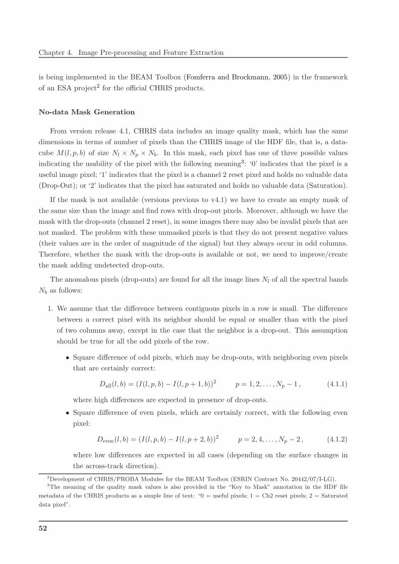
Chapter 4. Image Pre-processing and Feature Extraction
is being implemented in the BEAM Toolbox (Fomferra and Brockmann, 2005) in the framework
of an ESA project2 for the official CHRIS products.
No-data Mask Generation
From version release 4.1, CHRIS data includes an image quality mask, which has the same
dimensions in terms of number of pixels than the CHRIS image of the HDF file, that is, a data-
cube M(l, p, b) of size Nl × Np × Nb. In this mask, each pixel has one of three possible values
indicating the usability of the pixel with the following meaning3: ‘0’ indicates that the pixel is a
useful image pixel; ‘1’ indicates that the pixel is a channel 2 reset pixel and holds no valuable data
(Drop-Out); or ‘2’ indicates that the pixel has saturated and holds no valuable data (Saturation).
If the mask is not available (versions previous to v4.1) we have to create an empty mask of
the same size than the image and find rows with drop-out pixels. Moreover, although we have the
mask with the drop-outs (channel 2 reset), in some images there may also be invalid pixels that are
not masked. The problem with these unmasked pixels is that they do not present negative values
(their values are in the order of magnitude of the signal) but they always occur in odd columns.
Therefore, whether the mask with the drop-outs is available or not, we need to improve/create
the mask adding undetected drop-outs.
The anomalous pixels (drop-outs) are found for all the image lines Nl of all the spectral bands
Nb as follows:
1. We assume that the difference between contiguous pixels in a row is small. The difference
between a correct pixel with its neighbor should be equal or smaller than with the pixel
of two columns away, except in the case that the neighbor is a drop-out. This assumption
should be true for all the odd pixels of the row.
• Square difference of odd pixels, which may be drop-outs, with neighboring even pixels
that are certainly correct:
Dall(l, b) = (I(l, p, b) − I(l, p + 1, b))2 p = 1, 2, . . . ,Np − 1 , (4.1.1)
where high differences are expected in presence of drop-outs.
• Square difference of even pixels, which are certainly correct, with the following even
pixel:
Deven(l, b) = (I(l, p, b) − I(l, p+ 2, b))2 p = 2, 4, . . . ,Np − 2 , (4.1.2)
where low differences are expected in all cases (depending on the surface changes in
the across-track direction).
2Development of CHRIS/PROBA Modules for the BEAM Toolbox (ESRIN Contract No. 20442/07/I-LG).3The meaning of the quality mask values is also provided in the “Key to Mask” annotation in the HDF file
metadata of the CHRIS products as a simple line of text: “0 = useful pixels; 1 = Ch2 reset pixels; 2 = Saturated
data pixel”.
52

4.1. Pre-processing (I): TOA Radiance Corrections
2. Surface and vertical striping affect differences between contiguous columns, thus the ‘median’
is used to obtain a robust estimator of the average difference between pixels for the whole
line.
3. Finally, all odd pixels of the line are labeled as drop-out noise if the difference between
neighbours is 50% higher than between even pixels:
IFmedian(Dall(l, b))
median(Deven(l, b))> 1.5 THEN M(l, p, b) = 1 p = 1, 3, . . . ,Np (4.1.3)
Drop-out Correction
Once the drop-out errors have been detected, they must be corrected by using both spatial
and spectral information of the anomalous pixel and its neighbors. Each invalid pixel value is
replaced by a weighted average of the values of the neighboring pixels. In order to avoid the poor
performance of spatial filters (local average) in border or inhomogeneous areas (Larsen et al.,
1998; Garcia and Moreno, 2004), the contribution of each pixel (i, j) of a given neighborhood (C)
of size 3 × 3, is weighted by its similarity to the corrected pixel, I(l, p, b). In particular, this
similarity weight is the inverse of the Euclidean distance between the spectral signature of the
pixels, which is calculated locally using the nb upper and bottom spectral bands closer to the
corrected band b:
W (i, j) =
(
∑
k
(I(l, p, b) − I(l + i, p + j, b+ k))2
)−1/2
k = −nb, . . . ,−1, 1, . . . , nb . (4.1.4)
The final weight matrix, WC is modified to have zero values for the pixels not belonging to
the given neighborhood C and it is normalized in order to sum to one, i.e. , WC(i, j) =
C(i, j)W (i, j)/∑
i,j C(i, j)W (i, j). Finally, the new value of the drop-out is calculated as:
I(l, p, b) =∑
i,j
I(l + i, p+ j, b)WC (i, j) i, j = −1, 0, 1 . (4.1.5)
The result of this process is similar to a spatial interpolation but taking into account the simi-
larity with neighbors. It is worth noting that the values of bands with errors (indicated by the
CHRIS quality mask) are not considered during this process. The inputs required by the drop-out
correction algorithm are the CHRIS image, I, the improved quality mask, M , the definition of
the neighborhood, C, and the number of spectral bands nb used to compute the local spectral
distance.
The correction of the drop-out errors can be carried out independently of the vertical striping
correction. However, the vertical striping noise introduces different multiplicative factors in image
columns that can affect the new pixel value if the local average is performed by using contiguous
columns. Therefore, if drop-out correction is performed before the vertical striping correction,
only the values of the vertical neighbors (C2) must be used in order to avoid the effect of vertical
53

Chapter 4. Image Pre-processing and Feature Extraction
Figure 4.3: Vertical striping formation process from the combination of the non-uniform CCD pixel
response S(p, b) and the slit optical response Hx(p), which are constant in columns.
striping. After the vertical striping removal, it is possible to perform a second correction based
on the four-connected (C4) or eight-connected (C8) neighbors.
C2 =
(
0 1 0
0 0 0
0 1 0
)
C4 =
(
0 1 0
1 0 1
0 1 0
)
C8 =
(
1 1 1
1 0 1
1 1 1
)
(4.1.6)
Vertical Striping Correction
As it has been previously shown (cf. section 1.3), a spectral band b will be acquired by the
same row of CCD elements. Therefore, each image column p will be affected by a different CCD
pixel response S(p, b), and a different optical slit response Hx(p), which is equal for all spectral
bands. The combination of these non-uniform spatial responses, which are constant in columns,
superimposes a systematic pattern of noise organized by vertical lines (the formation of the stripe
noise is depicted in Fig. 4.3). Therefore, the relation between the desired at-sensor radiance,
LTOA(l, p, b), and the provided (radiometrically calibrated) product, I(l, p, b), can be expressed
from (1.3.4) as:
I(l, p, b) = LTOA(l, p, b)Hx(p)Hλ(b)S(p, b) + S0(l, p, b) = LTOA(l, p, b)ν(p, b) + S0(l, p, b) , (4.1.7)
where ν(p, b) is a multiplicative noise coming from the slit and CCD, and S0(l, p, b) represents
an additive noise. In the particular case of CHRIS, the provided level 1a images are radiomet-
rically corrected (so the units of I are radiance units instead of DN), and images processed at
version 4.1 of the CHRIS HDF files present an improved radiometric calibration (Cutter, 2004a;
Cutter and Johns, 2005b) which was poor in previous versions (underestimation up to a factor
two of the sensor measurements in the NIR). Therefore, one can assume that images present a
accurate spectral radiometric calibration with Hλ(b) ≃ 1, and are corrected of dark current off-
sets, thus making S0(l, p, b) negligible, i.e. remaining only random noise of zero mean and low
54

4.1. Pre-processing (I): TOA Radiance Corrections
(a) (b)
5.0
6.0
x 106
5.0
6.0
x 106
100 200 300 400 500 600 7000.9
1.0
Column index (p)
A
B
C
5.0
6.0
x 106
15.4
15.6
15.4
15.6
−0.1
0.0
100 200 300 400 500 600 7000.9
1.0
Column index (p)
A
B
D
C
E
Figure 4.4: Example of the processing steps of two different vertical striping correction methods pro-
posed by Barducci and Pippi (2001) (a) and Settle and Cutter (2005) (b): profiles of the last band of
CHRIS EI 060130 63A1 41 image taken over Heron Island.
amplitude. Hence, (4.1.7) is reduced to:
I(l, p, b) = LTOA(l, p, b)H(p)S(p, b) = LTOA(l, p, b)ν(p, b) . (4.1.8)
The objective of vertical striping (VS) correction methods is to estimate the correction factor,
ν(p, b) = H(p)S(p, b), of each spectral band to correct all the lines of this band. The main
assumption consists in considering that both slit (H) and CCD (S) contributions change from
one pixel to another (high spatial frequency) in the across-track (p) but are constant in the along-
track (l); while surface contribution (LTOA) presents smoother profiles (lower spatial frequencies)
in the across-track dimension.
Vertical striping correction methods. In the literature, all the vertical striping reduction
approaches take advantage of the constant noise factors in the image columns (Barducci and Pippi,
2001; Garcia and Moreno, 2004; Settle and Cutter, 2005; Mlsna and Becker, 2006). Basically, the
image is averaged in lines (along-track) and then the noise profile is estimated in the across-track
direction for each band. By averaging image lines (integrated line profile) the surface contribution
is smoothed, the additive random noise is cancelled, and the VS profile remains constant. Con-
sequently, the surface contribution presents lower spatial frequencies in the integrated line profile
and can be easily separated from the VS (high frequencies) applying a filter with a suited cut-off
frequency.
Figure 4.4a shows the three steps of the method proposed by Barducci and Pippi (2001):
A. Each band is averaged in lines (along-track direction) obtaining one integrated line profile
per band: α(p, b) =∫ Nl
1 I(l, p, b)dl = ν(p, b)∫ Nl
1 L(l, p, b)dl = ν(p, b)β(p, b).
55

Chapter 4. Image Pre-processing and Feature Extraction
B. A low pass filter (LPF) is applied using a moving-window algorithm that flattens the profile
α(p, b) by convolving it with a Gaussian weighting function w: β(p, b) = LPF{α(p, b)} =∫
w(p − k)α(p, b)dk. In this kind of filter, the cut-off frequency fc defines the standard
deviation of the Gaussian window, σ ∼ 1/fc.
C. Since β(p, b) mainly contains the surface contribution, the shape of the VS factors can be
obtained by the ratio ν(p, b) = α(p, b)/β(p, b). Thus, the corrected image is calculated as
L(l, p, b) = I(l, p, b)/ν(p, b).
Figure 4.4b shows the method that is used by SIRA Technology Ltd. to correct CHRIS images
(Settle and Cutter, 2005). The main difference with the previous method is the use of logarithms
to transform the multiplicative noise into additive noise in order to improve the filtering as follows:
A. Each band is averaged in lines obtaining one integrated line profile per band, α(p, b).
B. Log-transform the averaged profile: logα(p, b) ≡ log(α(p, b)) = log(ν(p, b)) + log(β(p, b))
C. Applying a low pass filter in order to eliminate high frequency variations (coming from the
noise ν) and estimate surface contribution: ˆlogβ(p, b) = LPF{logα(p, b)}.
D. Obtaining high frequency variations (considered as the noise): ˆlogν(p, b) = logα(p, b) −ˆlogβ(p, b)
E. The vertical striping factors are obtained calculating the inverse of the logarithm ν(p, b) =
exp( ˆlogν(p, b)).
Theoretically, the first approach should give poor results when filtering the line profile because it is
affected by a multiplicative noise and this is equivalent to a convolution in the frequency domain.
This is the main reason to propose the second approach but, in practice, both approaches give
equivalent results. This can be explained because features of the multiplicative noise, which
present a mean close to one (f = 0 and A = 1) and high frequency components of low amplitude
(high f and A ≃ 0.1). Therefore, when performing the convolution of the signal and noise in
the frequency domain, the power spectral density of the signal at low frequencies is not affected.
Since both methods provide equivalent results, we consider them as a single method and hereafter
we refer to them as the standard method.
The standard method can fail for several reasons, such as high amplitude changes in the VS,
which affect the performance of the low pass filter (wrong estimation of the surface contribu-
tion) producing an overestimation or underestimation in the correction factors of the neighboring
columns. Garcia and Moreno (2004) presented an iterative method that corrects the effect of
these high striping values. However, as proposed in the next section, these effects can be also
avoided using more advanced filtering techniques that use a weight function.
56

4.1. Pre-processing (I): TOA Radiance Corrections
Robust vertical striping correction method. One of the main drawbacks of the methods
proposed in the literature is the fact that they do not take into account the possible high frequency
components of the surface explicitly. In images presenting structures or patterns in the vertical
direction, the averaged profile α(p, b) may present high frequency contributions due to the surface.
This will be interpreted as vertical striping when estimating ν(p, b) (see the selected example in
Fig. 4.4), and some columns will be corrected with wrong values, worsening the final image.
The proposed correction method is also based on the hypothesis that the vertical disturbance
presents higher spatial frequencies than the surface radiance. However, it models the noise pattern
by suppressing the surface contribution in the across-track in two different ways: first, avoiding
the high frequency changes due to surface edges, and then subtracting the low frequency profile.
The surface can present high spatial frequencies due to: the surface texture, which has low am-
plitude changes; or changes in the land-cover type, which can produce great changes in amplitude
being a problem in the destriping process. In principle, in one spectral band, both the surface and
noise contributions are mixed and is not possible to distinguish which of them causes the changes
in the radiance amplitude between contiguous columns. However, the spectral signature of pixels
from current hyperspectral sensors can provide helpful information about the land cover changes.
Considering the spectra of two contiguous pixels, p1 and p2, just in the boundary between two
land-cover types, there are three factors affecting the spectral change: (i) differences between
the true spectra of both surfaces (in shape and magnitude); (ii) the different CCD sensitivity
S(p, b), which modulates the spectral signature as a multiplicative noise of low variance; and (iii)
the different multiplicative factor due to the slit H(p), which scales the magnitude of the whole
spectral signature. Among these three factors, the first one will produce the greater change, the
second one will be a second-order factor when comparing the spectral similarity, and the third one
will not affect the final result if the selected spectral distance is invariant to scaling by a positive
factor. Therefore, we can apply a filter in the across-track direction of the hyperspectral image in
order to find the surface borders that introduce high frequencies in the across-track profile. The
next sections explain how pixels corresponding to borders are not employed when computing the
integrated line profiles.
Spatio-Spectral Edge Detection. We propose a spatio-spectral filter based on spatial
convolution filters, which are commonly used in grayscale image processing, like the Derivation
filter or the Gradient-Roberts filter (Pratt, 2001). These spatial convolution filters which calculate
a weighted average of the cells in the current filter window. The spatial filter response, R, contains
the array of weighting coefficients used in the calculation. To find edges in the horizontal direction
(across-track) the edge detection matrix R of these methods can be(
−1 10 0
)
or(
1 −10 0
)
for the
derivation filter,(−1 0
0 1
)
or(0 −11 0
)
for the Roberts filter, or a combination of them. To apply these
techniques to hyperspectral images, taking into account the spectral dimension, it is not possible
to directly calculate the convolution of the edge detection matrix and the three-dimensional
hypercube. In our proposal, a spectral distance is first computed between the spectrum of the
57
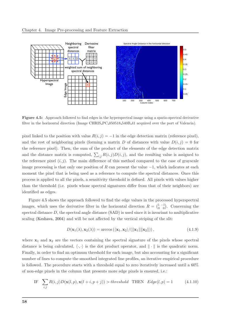
Chapter 4. Image Pre-processing and Feature Extraction
X
X
S A D
0 0 0
1 -1 0
0 0 0
Derivativefilter
matrix
Neighboringspectraldistances
weighted sum of neighboring spectral distances
HyperspectralImage
Edge
Im
age
Column index
Spectral Angle Distance in the horizontal direction
100 200 300 400 500 600 700
0.05
0.1
0.15
0.2
0.25
0.3
0.35
0.4
0.45
0.5
Figure 4.5: Approach followed to find edges in the hyperspectral image using a spatio-spectral derivative
filter in the horizontal direction (Image CHRIS PC 050518 540B 41 acquired over the port of Valencia).
pixel linked to the position with value R(i, j) = −1 in the edge detection matrix (reference pixel),
and the rest of neighboring pixels (forming a matrix D of distances with value D(i, j) = 0 for
the reference pixel). Then, the sum of the product of the elements of the edge detection matrix
and the distance matrix is computed,∑
i,j R(i, j)D(i, j), and the resulting value is assigned to
the reference pixel (i, j). The main difference of this method compared to the case of grayscale
image processing is that only one position of R can present the value −1, which indicates at each
moment the pixel that is being used as a reference to compute the spectral distances. Once this
process is applied to all the pixels, a sensitivity threshold is defined. All pixels with values higher
than the threshold (i.e. pixels whose spectral signatures differ from that of their neighbors) are
identified as edges.
Figure 4.5 shows the approach followed to find the edge values in the processed hyperspectral
images, which uses the derivative filter in the horizontal direction R =(
1 −10 0
)
. Concerning the
spectral distance D, the spectral angle distance (SAD) is used since it is invariant to multiplicative
scaling (Keshava, 2004) and will be not affected by the vertical striping of the slit:
D(x1(λ),x2(λ)) = arccos (〈x1,x2〉/(‖x1‖‖x2‖)) , (4.1.9)
where x1 and x2 are the vectors containing the spectral signature of the pixels whose spectral
distance is being calculated, 〈·, ·〉 is the dot product operator, and ‖ · ‖ is the quadratic norm.
Finally, in order to find an optimum threshold for each image, but also accounting for a significant
number of lines to compute the smoothed integrated line profiles, an iterative empirical procedure
is followed. The procedure starts with a threshold equal to zero iteratively increased until a 60%
of non-edge pixels in the column that presents more edge pixels is ensured, i.e.:
IF∑
i,j
R(i, j)D(x(l, p),x(l + i, p+ j)) > threshold THEN Edge(l, p) = 1 (4.1.10)
58
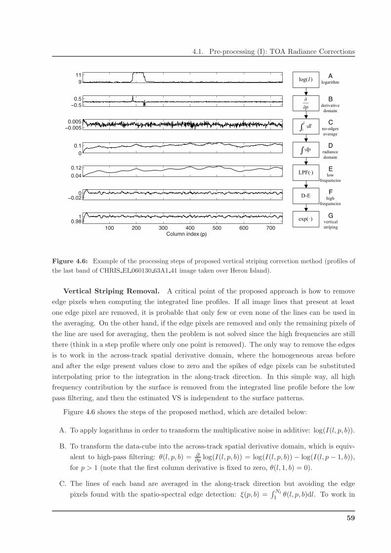
4.1. Pre-processing (I): TOA Radiance Corrections
(p)
log( )I
p
1·L
dl
·dp
LPF(·)
D-E
exp(· )
Alogarithm
Bderivative
domain
Cno-edges
average
Elow
frequencies
Fhigh
frequencies
Dradiance
domain
Gvertical
striping
Figure 4.6: Example of the processing steps of proposed vertical striping correction method (profiles of
the last band of CHRIS EI 060130 63A1 41 image taken over Heron Island).
Vertical Striping Removal. A critical point of the proposed approach is how to remove
edge pixels when computing the integrated line profiles. If all image lines that present at least
one edge pixel are removed, it is probable that only few or even none of the lines can be used in
the averaging. On the other hand, if the edge pixels are removed and only the remaining pixels of
the line are used for averaging, then the problem is not solved since the high frequencies are still
there (think in a step profile where only one point is removed). The only way to remove the edges
is to work in the across-track spatial derivative domain, where the homogeneous areas before
and after the edge present values close to zero and the spikes of edge pixels can be substituted
interpolating prior to the integration in the along-track direction. In this simple way, all high
frequency contribution by the surface is removed from the integrated line profile before the low
pass filtering, and then the estimated VS is independent to the surface patterns.
Figure 4.6 shows the steps of the proposed method, which are detailed below:
A. To apply logarithms in order to transform the multiplicative noise in additive: log(I(l, p, b)).
B. To transform the data-cube into the across-track spatial derivative domain, which is equiv-
alent to high-pass filtering: θ(l, p, b) = ∂∂p log(I(l, p, b)) = log(I(l, p, b)) − log(I(l, p − 1, b)),
for p > 1 (note that the first column derivative is fixed to zero, θ(l, 1, b) = 0).
C. The lines of each band are averaged in the along-track direction but avoiding the edge
pixels found with the spatio-spectral edge detection: ξ(p, b) =∫ Nl
1 θ(l, p, b)dl. To work in
59

Chapter 4. Image Pre-processing and Feature Extraction
the derivative domain has allowed our method to avoid edge pixels, and it also leads to
increase the noise level temporarily because the surface power spectrum is concentrated in
the low frequency region, whereas the vertical striping is spread all over the spatial frequency
spectrum (Othman and Qian, 2006). Nevertheless, if the LPF is applied in the derivative
domain, the committed errors by the LPF will accumulate throughout the integration in
the across-track direction. Therefore, after applying the along-track LPF, data is integrated
across-track to retrieve the signal in the radiance domain.
D. Integration in the across-track direction (cumulative sum in p): φ(p, b) =∑p
i=1 ξ(i, b), i.e.
the integration bias is corrected at the end of the process.
E. To apply a LPF in the across-track direction in order to eliminate the high frequency varia-
tions coming from the noise ν and estimate the surface contribution: ϕ(p, b) = LPF{φ(p, b)}.
F. To obtain the high frequency variations (considered to be the noise) by subtracting the low
frequencies: ψ(p, b) = φ(p, b) − ϕ(p, b). The error committed during the integration process
consists in a constant value for each band. Nevertheless, as the vertical striping is corrected
independently for each band, the vertical striping in the logarithmic domain should present
zero mean (gain close to 1 in the radiance image). Therefore, the offset errors are corrected
subtracting the mean value: ψ(p, b) = ψ(p, b) − 1Np
∑
p ψ(p, b).
G. Finally, the VS factors are obtained calculating the inverse of the logarithm ν(p, b) =
exp(ψ(p, b)).
Multiangular Vertical Striping Removal. Thanks to the sequential acquisition of CHRIS
of the same scene from five different angles, we can also improve the robustness of the proposed
algorithm using together all the multiangular images of one acquisition. As mentioned before, the
VS due to the instrument slit is temperature-dependent. Although temperature recorded for dif-
ferent acquisitions has shown differences higher than 8◦C, the changes are less than 0.5◦C within
a single acquisition (5 multi-angular images). Therefore, images of one acquisition present the
same vertical striping pattern while they are recording different spatial patterns from the same
Earth area (due to perspective, platform motion and Earth rotation). One can take advantage of
this fact in order to improve the estimation of the vertical striping by considering the five images
as a single longer hyperspectral image, which is formed by stacking the multiangular images in
the along-track direction, i.e. an hyper-cube with the same number of columns Np and bands Nb,
but with 5 ×Nl lines with different spatial distribution of similar surface types (similar spectra).
When processing together a higher number of lines, the surface contribution is smoother and the
estimation of the VS is more accurate.
Vertical Striping Characterization and Correction of the Slit Effect. An extensive anal-
ysis of the performance of the proposed vertical striping method was carried out with more than
60

4.1. Pre-processing (I): TOA Radiance Corrections
300 CHRIS images of several acquisition modes in (Gomez-Chova et al., 2006a; Gomez-Chova et al.,
2008). Details about the vertical striping results will be omitted in this Thesis, but a result of great
value is the characterization of the vertical striping and its dependence on temperature. With this
purpose, we corrected a significant number of CHRIS images of the database obtaining an estima-
tion of the vertical striping pattern, ν(p, b) = H(p)S(p, b), per image. The sensitivity of the CCD
array, S(p, b), is assumed to be characterized by a Gaussian distribution with unit mean. How-
ever, by applying the logarithmic transformation to the estimated VS, the multiplicative nature
of both terms is changed to additive one, log(ν(p, b)) = log(H(p)) + log(S(p, b)), where the term
log(S(p, b)) can be safely considered additive noise with zero mean distribution. As a consequence,
the VS profile due to the slit, which is constant in columns, can be obtained by averaging in the
spectral direction of the CCD and then reverting the logarithm: H(p) = exp(∫ Nb
1 log(ν(p, b))db).
Moreover, the slit-VS profiles of the five angular images can be averaged to obtain only one H(p)
per acquisition, which will be associated to the platform temperature for this given acquisition:
H(p, T ). Changes in temperature produce an expansion of the slit, changing its width and moving
the image of the slit across the detector. These two effects produce a scaling of the slit-VS factors
and a shift of its shape in the across-track direction, respectively, causing a temperature dependent
vertical striping. Figure 4.7, on the left side, shows a peak of the obtained H(p) profiles for all
the analyzed Mode 2 acquisitions (Mode 2 is shown because it is not binned and presents higher
across-track resolution than Mode 1). The ‘∗’ symbols represent the actual H(p) values for each
pixel column p, and the curves (continuous lines) are the corresponding spline interpolations in
the across-track direction x, which provide a continuous subpixel resolution model of the striping
H(x) for each measured temperature T : H(x, T ). The curves clearly show the shift and scaling
of the VS amplitude with temperature. Taking the VS at T0 = 5.5◦C as a reference, we compute
the shift in the across-track looking for the lag, ∆x(T ), of the maximum of the cross-correlation
sequence between the analyzed vertical striping, H(x, T ), and the reference one, H(x, T0). Once
the shift is corrected, the scaling factor GH(T ) is computed as the slope of the linear regression
that better fits H(x, T ) with H(x, T0) in a least-squares sense. In the central and right plots of
Fig. 4.7 we represent the shift ∆x(T ) and scale GH(T ) of the slit-VS as a function of temperature,
respectively.
The estimated ∆x(T ) and GH(T ) values are used to compensate the shift and scale of the
slit-VS H(x, T ) and obtain the corresponding slit-VS for each acquisition of the database, but
expressed at the reference temperature T0. The average of all these curves provides us a model
of the “real” slit-VS at the reference temperature, denoted by H(x), minimizing the estimation
errors. The modeled slit-VS for a given temperature T can be recovered from H(x) as:
H(x, T ) = GH(T )H(x− ∆x(T )) (4.1.11)
where ∆x(T0) = 0 and GH(T0) = 1. The value for a given pixel column p is obtained integrating
the width of the pixel photo-sensible area:
H(p, T ) =
∫ p+1/2
p−1/2H(x, T )dx (4.1.12)
61
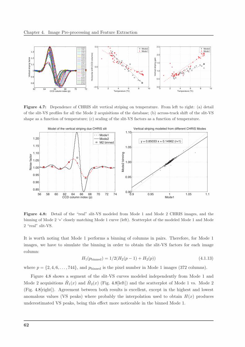
Chapter 4. Image Pre-processing and Feature Extraction
62 64 66 68 70 72
0.8
0.9
1
1.1
1.2
1.3
CCD column index (p)
Ver
tical
str
ipin
g fa
ctor
2.68ºC 2.8ºC3.08ºC 3.7ºC3.85ºC3.99ºC4.14ºC4.59ºC4.67ºC4.68ºC 5.3ºC5.51ºC5.67ºC5.84ºC5.99ºC 6.3ºC6.82ºC7.15ºC 7.9ºC8.22ºC8.63ºC8.64ºC8.66ºC8.73ºC
0 2 4 6 8 10−0.5
0.0
0.5
Temperature (ºC)H
orizonta
l shift (C
CD
colu
mns)
Mode2
Mode1
0 2 4 6 8 100.0
0.5
1.0
1.5
2.0
2.5
Temperature (ºC)
Vert
ical str
ipin
g g
ain
Mode2
Mode1
Figure 4.7: Dependence of CHRIS slit vertical striping on temperature. From left to right: (a) detail
of the slit-VS profiles for all the Mode 2 acquisitions of the database; (b) across-track shift of the slit-VS
shape as a function of temperature; (c) scaling of the slit-VS factors as a function of temperature.
56 58 60 62 64 66 68 70 72 74
0.85
0.90
0.95
1.00
1.05
1.10
1.15
1.20
Model of the vertical striping due CHRIS slit
CCD column index (p)
No
ise
fa
cto
r
Mode1
Mode2
M2 binned
0.9 0.95 1 1.05 1.10.90
0.95
1.00
1.05
1.10
Mode1
Mo
de
2 b
inn
ing
Vertical striping modeled from different CHRIS Modes
y = 0.85033 x + 0.14962 (r=1)
Figure 4.8: Detail of the “real” slit-VS modeled from Mode 1 and Mode 2 CHRIS images, and the
binning of Mode 2 ‘∗’ closely matching Mode 1 curve (left). Scatterplot of the modeled Mode 1 and Mode
2 “real” slit-VS.
It is worth noting that Mode 1 performs a binning of columns in pairs. Therefore, for Mode 1
images, we have to simulate the binning in order to obtain the slit-VS factors for each image
column:
H1(pbinned) = 1/2(H2(p− 1) +H2(p)) (4.1.13)
where p = {2, 4, 6, . . . , 744}, and pbinned is the pixel number in Mode 1 images (372 columns).
Figure 4.8 shows a segment of the slit-VS curves modeled independently from Mode 1 and
Mode 2 acquisitions H1(x) and H2(x) (Fig. 4.8[left]) and the scatterplot of Mode 1 vs. Mode 2
(Fig. 4.8[right]). Agreement between both results is excellent, except in the highest and lowest
anomalous values (VS peaks) where probably the interpolation used to obtain H(x) produces
underestimated VS peaks, being this effect more noticeable in the binned Mode 1.
62
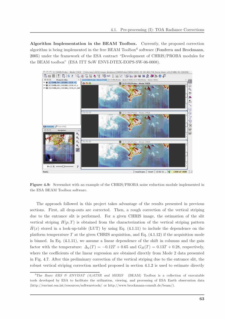
4.1. Pre-processing (I): TOA Radiance Corrections
Algorithm Implementation in the BEAM Toolbox. Currently, the proposed correction
algorithm is being implemented in the free BEAM Toolbox4 software (Fomferra and Brockmann,
2005) under the framework of the ESA contract “Development of CHRIS/PROBA modules for
the BEAM toolbox” (ESA ITT SoW ENVI-DTEX-EOPS-SW-06-0008).
Figure 4.9: Screenshot with an example of the CHRIS/PROBA noise reduction module implemented in
the ESA BEAM Toolbox software.
The approach followed in this project takes advantage of the results presented in previous
sections. First, all drop-outs are corrected. Then, a rough correction of the vertical striping
due to the entrance slit is performed. For a given CHRIS image, the estimation of the slit
vertical striping H(p, T ) is obtained from the characterization of the vertical striping pattern
H(x) stored in a look-up-table (LUT) by using Eq. (4.1.11) to include the dependence on the
platform temperature T at the given CHRIS acquisition, and Eq. (4.1.12) if the acquisition mode
is binned. In Eq. (4.1.11), we assume a linear dependence of the shift in columns and the gain
factor with the temperature: ∆x(T ) = −0.12T + 0.65 and GH(T ) = 0.13T + 0.28, respectively,
where the coefficients of the linear regression are obtained directly from Mode 2 data presented
in Fig. 4.7. After this preliminary correction of the vertical striping due to the entrance slit, the
robust vertical striping correction method proposed in section 4.1.2 is used to estimate directly
4The Basic ERS & ENVISAT (A)ATSR and MERIS (BEAM) Toolbox is a collection of executable
tools developed by ESA to facilitate the utilization, viewing, and processing of ESA Earth observation data
(http://envisat.esa.int/resources/softwaretools/ or http://www.brockmann-consult.de/beam/).
63

Chapter 4. Image Pre-processing and Feature Extraction
from the image (or multiangular acquisition) the remaining vertical striping for each band ν(p, b).
Finally, obtained factors are used to correct the image column values .
Figure 4.9 shows an screenshot of the ESA BEAM Toolbox software. In this example we
display the same area for the original CHRIS product (top), the image corrected with the al-
gorithm implemented by Settle and Cutter (2005) (middle), and the image processed with the
CHRIS/PROBA noise reduction module proposed in this work and implemented in the BEAM
Toolbox (bottom). One can easily appreciate how the vertical patterns are reduced from top to
bottom pictures.
4.2 Pre-processing (II): TOA Reflectance
Once the data have been corrected of errors and uncertainties, these data are independent of
differences in sensor system conditions. Hence, it is no longer necessary to express this information
in terms of the image-sensor lines and columns. Now, the multispectral image can be expressed
in terms of pixels with spatial coordinates (x, y), and the spectral information of each sensor
channel in terms of the central wavelength λb and bandwidth Λb of the band. Only for some precise
spectral calculations, which require the exact central wavelength for each pixel, information about
the original detector elements will be used, mainly when dealing with narrow absorption bands
where a small spectral shift affects the measure.
As already mentioned, both MERIS and CHRIS Level 1b products are provided in top of
the atmosphere (TOA) radiance. The corrected TOA radiance is further processed in order to
estimate TOA reflectance. This allows us to remove in practice the dependence on particular
illumination conditions (day of the year and angular configuration) and illumination effects due
to rough terrain (cosine correction), since the method is intended to work under many situations.
TOA apparent reflectance is estimated as follows:
ρTOA(x, y, λ) =πLTOA(x, y, λ)
µs(x, y)F0(λ), (4.2.1)
where LTOA(x, y, λ) is the provided at-sensor upward radiance at the image location (x, y), F0(λ)
is the extraterrestrial instantaneous solar irradiance, and µs(x, y) is the cosine of the angle between
the illumination direction (solar zenith angle) and the vector perpendicular to the surface. Finally,
the Sun irradiance, F0(λ), is taken from Thuillier et al. (2003), corrected for the acquisition day,
and convolved with the spectral response of the sensor channels (see Fig. 4.10).
4.2.1 Day-of-Year Correction
The largest source of variation in F0 at the TOA is the orbit of the Earth around the Sun
(cf. section 1.1.2). The Sun is located at one of the foci of the Earth’s orbit (an ellipse with
eccentricity ǫ = 0.01673), and the value of F0 is expected to vary as the reciprocal of the Earth-
Sun distance squared. The mean Earth-Sun distance is referred to as 1 Astronomical Unit (AU)
64
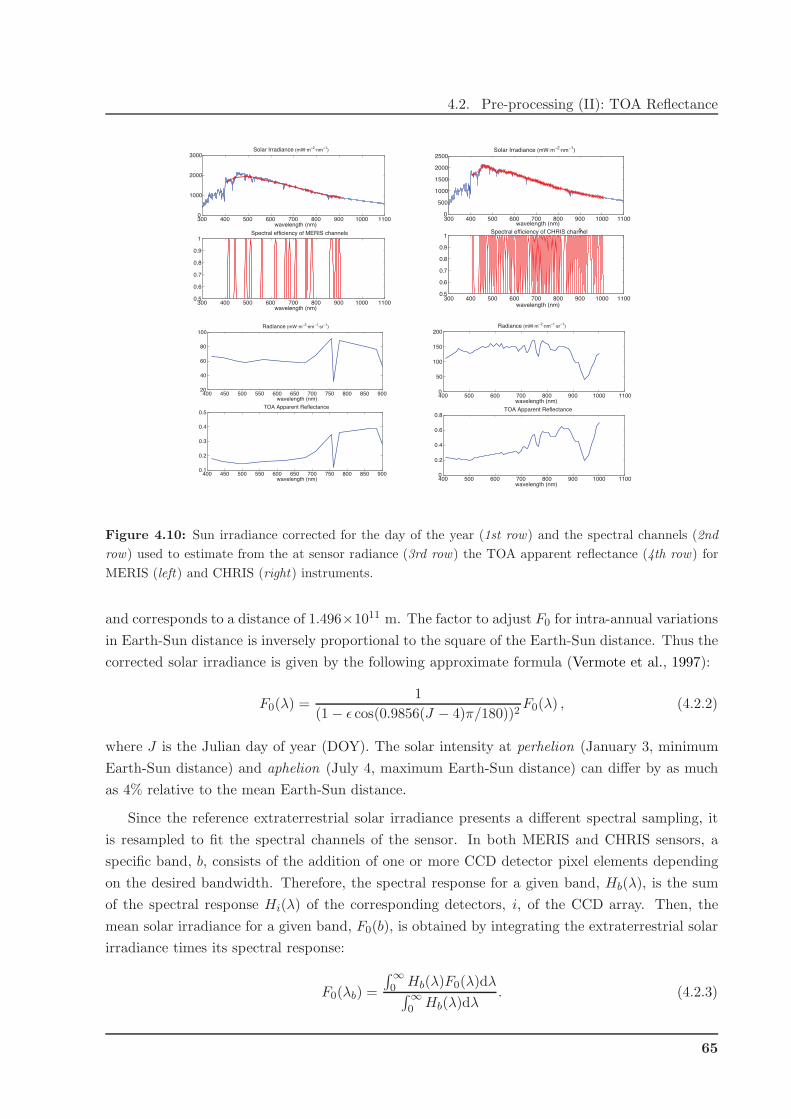
4.2. Pre-processing (II): TOA Reflectance
300 400 500 600 700 800 900 1000 11000
1000
2000
3000Solar Irradiance (mW·m
−2·nm
−1)
wavelength (nm)
300 400 500 600 700 800 900 1000 11000.5
0.6
0.7
0.8
0.9
1Spectral efficiency of MERIS channels
wavelength (nm)
300 400 500 600 700 800 900 1000 11000
500
1000
1500
2000
2500Solar Irradiance (mW·m
−2·nm
−1)
wavelength (nm)
300 400 500 600 700 800 900 1000 11000.5
0.6
0.7
0.8
0.9
1Spectral efficiency of CHRIS channels
wavelength (nm)
400 450 500 550 600 650 700 750 800 850 90020
40
60
80
100Radiance (mW ⋅m
−2⋅nm
−1⋅sr
−1)
wavelength (nm)
400 450 500 550 600 650 700 750 800 850 9000.1
0.2
0.3
0.4
0.5TOA Apparent Reflectance
wavelength (nm)
400 500 600 700 800 900 1000 11000
50
100
150
200Radiance (mW⋅m
−2⋅nm
−1⋅sr
−1)
wavelength (nm)
400 500 600 700 800 900 1000 11000
0.2
0.4
0.6
0.8TOA Apparent Reflectance
wavelength (nm)
Figure 4.10: Sun irradiance corrected for the day of the year (1st row) and the spectral channels (2nd
row) used to estimate from the at sensor radiance (3rd row) the TOA apparent reflectance (4th row) for
MERIS (left) and CHRIS (right) instruments.
and corresponds to a distance of 1.496×10¹¹ m. The factor to adjust F0 for intra-annual variations
in Earth-Sun distance is inversely proportional to the square of the Earth-Sun distance. Thus the
corrected solar irradiance is given by the following approximate formula (Vermote et al., 1997):
F0(λ) =1
(1 − ǫ cos(0.9856(J − 4)π/180))2F0(λ) , (4.2.2)
where J is the Julian day of year (DOY). The solar intensity at perhelion (January 3, minimum
Earth-Sun distance) and aphelion (July 4, maximum Earth-Sun distance) can differ by as much
as 4% relative to the mean Earth-Sun distance.
Since the reference extraterrestrial solar irradiance presents a different spectral sampling, it
is resampled to fit the spectral channels of the sensor. In both MERIS and CHRIS sensors, a
specific band, b, consists of the addition of one or more CCD detector pixel elements depending
on the desired bandwidth. Therefore, the spectral response for a given band, Hb(λ), is the sum
of the spectral response Hi(λ) of the corresponding detectors, i, of the CCD array. Then, the
mean solar irradiance for a given band, F0(b), is obtained by integrating the extraterrestrial solar
irradiance times its spectral response:
F0(λb) =
∫∞0 Hb(λ)F0(λ)dλ∫∞0 Hb(λ)dλ
. (4.2.3)
65

Chapter 4. Image Pre-processing and Feature Extraction
Digital Elevation Model (m)
0
200
400
600
800
1000
1200
1400
1600
1800
2000
Cosine correction: Illumination effects in rough terrain.
0.6
0.65
0.7
0.75
0.8
0.85
0.9
0.95
1
Figure 4.11: Left : DEM altitude of the BR-2003-07-14image. Right : Cosine of the angle between the
illumination vector and a vector perpendicular to the surface (cosine correction).
In CHRIS sensor, the theoretical full-width half-maximum (FWHM) of the instrument line-
spread functions correspond to spectral resolutions of 1.25 nm at 415 nm, increasing to 11.25 nm
at 1050 nm. In MERIS, the CCD covers the spectral range with a nominal 1.25 nm spectral
sampling interval and with a FWHM equal to 1.25 nm. For both instruments, one could assume
that Hi(λ) is a Gaussian response function whose width is equal to the FWHM of each element
i, and sum up all the elements of the band. In this Thesis, the spectral response of a band,
Hb(λ) is approximated as a bell-shaped function (that combines properties of both Gaussian and
trapezoidal functions) depending on the mid-wavelength, λb, and the bandwidth, Λb, of the band,
directly:
Hb(λ) =1
1 + |2(λ− λb)/Λb|4λb − Λb < λ < λb + Λb, (4.2.4)
where both the exact mid-wavelength and the bandwidth values for each channel are included in
the image metadata.
4.2.2 Rough Surface Correction
In this Thesis, the angle between the illumination direction and the vector perpendicular to
the surface, which defines µs(x, y), is computed in a different way depending on the sensor:
• In MERIS, it is computed for each pixel using the Sun Azimuth and Sun Zenith angles,
which are available in the Tie Point Location and Auxiliary Data of the MERIS product,
and the vector perpendicular to the surface, which can be computed from a Digital Ele-
vation Model (DEM). The free GETASSE30 DEM included in the BEAM ESA software
(Fomferra and Brockmann, 2005) may be used for this purpose (Fig. 4.11). In this step,
however, we assume a flat surface because, by using a DEM, illumination effects in the
surface are corrected but the characteristics of clouds over rough terrain may change.
• In CHRIS, this correction is approximated by the Solar Zenith Angle provided in the CHRIS
HDF file attributes since, due to the small field of view of CHRIS, one can assume a flat
66
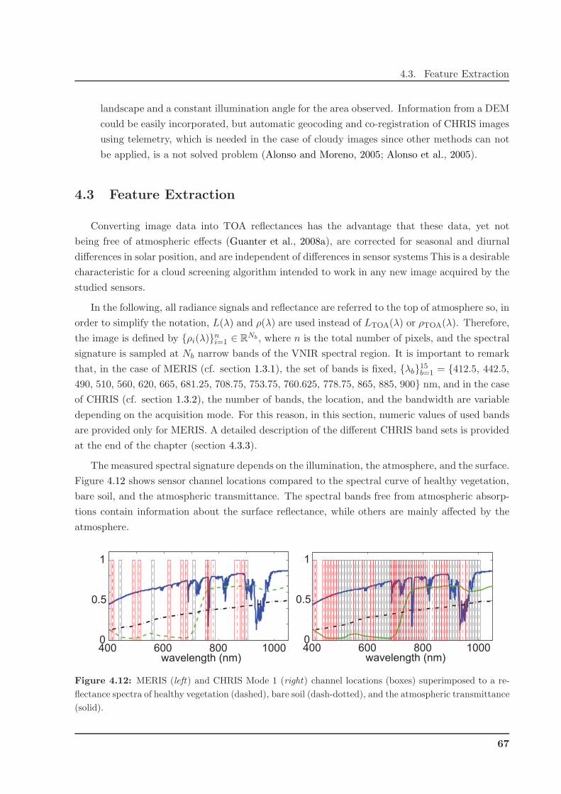
4.3. Feature Extraction
landscape and a constant illumination angle for the area observed. Information from a DEM
could be easily incorporated, but automatic geocoding and co-registration of CHRIS images
using telemetry, which is needed in the case of cloudy images since other methods can not
be applied, is a not solved problem (Alonso and Moreno, 2005; Alonso et al., 2005).
4.3 Feature Extraction
Converting image data into TOA reflectances has the advantage that these data, yet not
being free of atmospheric effects (Guanter et al., 2008a), are corrected for seasonal and diurnal
differences in solar position, and are independent of differences in sensor systems This is a desirable
characteristic for a cloud screening algorithm intended to work in any new image acquired by the
studied sensors.
In the following, all radiance signals and reflectance are referred to the top of atmosphere so, in
order to simplify the notation, L(λ) and ρ(λ) are used instead of LTOA(λ) or ρTOA(λ). Therefore,
the image is defined by {ρi(λ)}ni=1 ∈ R
Nb , where n is the total number of pixels, and the spectral
signature is sampled at Nb narrow bands of the VNIR spectral region. It is important to remark
that, in the case of MERIS (cf. section 1.3.1), the set of bands is fixed, {λb}15b=1 = {412.5, 442.5,
490, 510, 560, 620, 665, 681.25, 708.75, 753.75, 760.625, 778.75, 865, 885, 900} nm, and in the case
of CHRIS (cf. section 1.3.2), the number of bands, the location, and the bandwidth are variable
depending on the acquisition mode. For this reason, in this section, numeric values of used bands
are provided only for MERIS. A detailed description of the different CHRIS band sets is provided
at the end of the chapter (section 4.3.3).
The measured spectral signature depends on the illumination, the atmosphere, and the surface.
Figure 4.12 shows sensor channel locations compared to the spectral curve of healthy vegetation,
bare soil, and the atmospheric transmittance. The spectral bands free from atmospheric absorp-
tions contain information about the surface reflectance, while others are mainly affected by the
atmosphere.
400 600 800 10000
0.5
1
wavelength (nm)400 600 800 10000
0.5
1
wavelength (nm)
Figure 4.12: MERIS (left) and CHRIS Mode 1 (right) channel locations (boxes) superimposed to a re-
flectance spectra of healthy vegetation (dashed), bare soil (dash-dotted), and the atmospheric transmittance
(solid).
67
Chapter 4. Image Pre-processing and Feature Extraction
At this step, rather than working with the spectral reflectance only, physically-inspired fea-
tures are used in order to increase the separability of clouds and surface covers, which is a common
strategy in remote sensing classification (Gomez-Chova et al., 2003c,a). These features are ex-
tracted independently from the channels that are free from strong gaseous absorptions (λb ⊂ BS)
and from the channels substantially affected by the atmosphere (λb ⊂ BA). In the case of MERIS,
which presents a fixed band configuration, the atmospheric channels, BA, are b = {11, 15} and
the surface channels, BS , are b = {1, . . . , 10, 12, . . . , 14}. A detailed analysis of the extracted
features is given in the following subsections. For illustration purposes, only the extracted fea-
tures from one CHRIS image (CHRIS-BR-050717-576C-41, section 7.1.1) and one MERIS image
(BR-2003-07-14, section 7.2.1) are provided.
4.3.1 Surface Spectral Features
Regarding reflectance of the surface, one of the main characteristics of clouds is that they
present bright and white spectra (Fig. 4.13). We can exploit bands in BS in order to extract
information about the target reflectance, i.e. cloud brightness and cloud whiteness for cloudy
pixels:
• A bright spectrum means that the intensity of the spectral curve (related to the albedo)
should present relatively high values. Therefore, cloud brightness is calculated for each pixel
as the integral of spectrum, fBr =∫
ρ(λ)dλ, which can be approximated with a trapezoidal
numerical integration:
fBr =1
λmax − λmin
∑
λb⊂BS
ρ(λb+1) + ρ(λb)
2(λb+1 − λb), (4.3.1)
which differs from the average of the spectral channels since it takes into account the dis-
tribution of the energy along the spectrum.
• A white spectrum means that the spectral signature must be flat along the spectrum. The
first derivative of the spectral curve should present low values, but noise and calibration
errors may reduce the accuracy in the estimation of the spectrum flatness when computing
the spectral derivative in channels with similar wavelengths. Therefore, we compute for each
pixel the deviation from the flatness as the (trapezoidal approximate) integral of e(λ) =
|ρ(λ) − fBr|:fWh =
1
λmax − λmin
∑
λb⊂BS
e(λb+1) + e(λb)
2(λb+1 − λb) (4.3.2)
Further surface features can be obtained by considering independently the VIS (λVIS ∈ [400−700] nm) and NIR (λNIR ∈ [700−1000] nm) spectral ranges, where surface covers present different
reflectance properties. Therefore, instead of working with fBr and fWh, we can obtain 2+2 features
from (4.3.1) and (4.3.2) respectively: fBr,VIS and fWh,VIS, computed using λb ⊂ (BS ∩ VIS); and
68
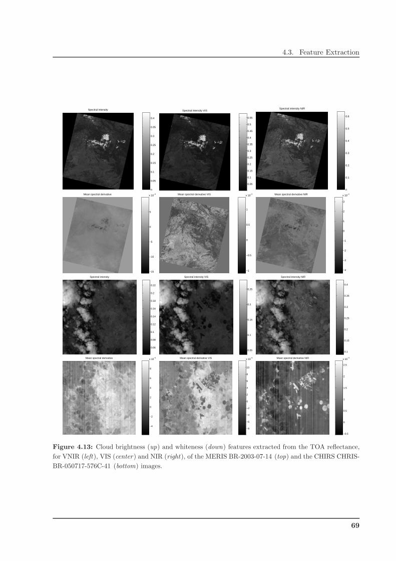
4.3. Feature Extraction
Spectral intensity
0
0.05
0.1
0.15
0.2
0.25
0.3
0.35
0.4
Spectral intensity VIS
0.05
0.1
0.15
0.2
0.25
0.3
0.35
0.4
0.45
0.5
0.55
Spectral intensity NIR
0
0.1
0.2
0.3
0.4
0.5
0.6
Mean spectral derivative
−15
−10
−5
0
5
x 10−4 Mean spectral derivative VIS
−1
−0.5
0
0.5
1
x 10−3 Mean spectral derivative NIR
−4
−3
−2
−1
0
1
2
3
x 10−3
Spectral intensity
0.06
0.08
0.1
0.12
0.14
0.16
0.18
0.2
0.22
Spectral intensity VIS
0.05
0.1
0.15
0.2
0.25
Spectral intensity NIR
0.1
0.15
0.2
0.25
0.3
0.35
0.4
Mean spectral derivative
−4
−2
0
2
4
6
8
x 10−4 Mean spectral derivative VIS
−8
−6
−4
−2
0
2
4
6
8
10
x 10−4 Mean spectral derivative NIR
−0.5
0
0.5
1
1.5
2
2.5
x 10−3
Figure 4.13: Cloud brightness (up) and whiteness (down) features extracted from the TOA reflectance,
for VNIR (left), VIS (center) and NIR (right), of the MERIS BR-2003-07-14 (top) and the CHIRS CHRIS-
BR-050717-576C-41 (bottom) images.
69
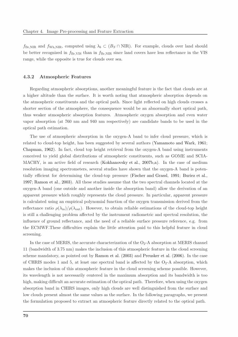
Chapter 4. Image Pre-processing and Feature Extraction
fBr,NIR and fWh,NIR, computed using λb ⊂ (BS ∩ NIR). For example, clouds over land should
be better recognized in fBr,VIS than in fBr,NIR since land covers have less reflectance in the VIS
range, while the opposite is true for clouds over sea.
4.3.2 Atmospheric Features
Regarding atmospheric absorptions, another meaningful feature is the fact that clouds are at
a higher altitude than the surface. It is worth noting that atmospheric absorption depends on
the atmospheric constituents and the optical path. Since light reflected on high clouds crosses a
shorter section of the atmosphere, the consequence would be an abnormally short optical path,
thus weaker atmospheric absorption features. Atmospheric oxygen absorption and even water
vapor absorption (at 760 nm and 940 nm respectively) are candidate bands to be used in the
optical path estimation.
The use of atmospheric absorption in the oxygen-A band to infer cloud pressure, which is
related to cloud-top height, has been suggested by several authors (Yamamoto and Wark, 1961;
Chapman, 1962). In fact, cloud top height retrieval from the oxygen-A band using instruments
conceived to yield global distributions of atmospheric constituents, such as GOME and SCIA-
MACHY, is an active field of research (Kokhanovsky et al., 2007b,a). In the case of medium
resolution imaging spectrometers, several studies have shown that the oxygen-A band is poten-
tially efficient for determining the cloud-top pressure (Fischer and Grassl, 1991; Buriez et al.,
1997; Ramon et al., 2003). All these studies assume that the two spectral channels located at the
oxygen-A band (one outside and another inside the absorption band) allow the derivation of an
apparent pressure which roughly represents the cloud pressure. In particular, apparent pressure
is calculated using an empirical polynomial function of the oxygen transmission derived from the
reflectance ratio ρ(λin)/ρ(λout). However, to obtain reliable estimations of the cloud-top height
is still a challenging problem affected by the instrument radiometric and spectral resolution, the
influence of ground reflectance, and the need of a reliable surface pressure reference, e.g. from
the ECMWF.These difficulties explain the little attention paid to this helpful feature in cloud
screening.
In the case of MERIS, the accurate characterization of the O2-A absorption at MERIS channel
11 (bandwidth of 3.75 nm) makes the inclusion of this atmospheric feature in the cloud screening
scheme mandatory, as pointed out by Ramon et al. (2003) and Preusker et al. (2006). In the case
of CHRIS modes 1 and 5, at least one spectral band is affected by the O2-A absorption, which
makes the inclusion of this atmospheric feature in the cloud screening scheme possible. However,
its wavelength is not necessarily centered in the maximum absorption and its bandwidth is too
high, making difficult an accurate estimation of the optical path. Therefore, when using the oxygen
absorption band in CHIRS images, only high clouds are well distinguished from the surface and
low clouds present almost the same values as the surface. In the following paragraphs, we present
the formulation proposed to extract an atmospheric feature directly related to the optical path.
70
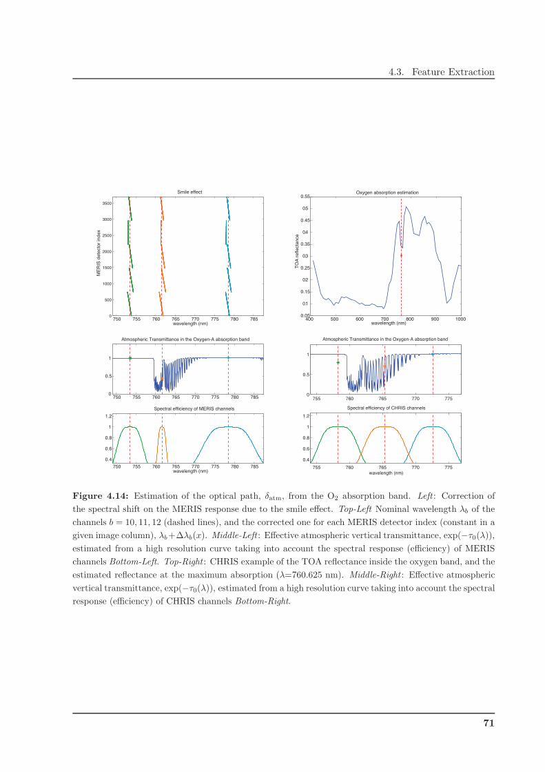
4.3. Feature Extraction
750 755 760 765 770 775 780 7850
500
1000
1500
2000
2500
3000
3500
wavelength (nm)
ME
RIS
dete
cto
r in
dex
Smile effect
400 500 600 700 800 900 10000.05
0.1
0.15
0.2
0.25
0.3
0.35
0.4
0.45
0.5
0.55Oxygen absorption estimation
wavelength (nm)
TO
A r
eflecta
nce
750 755 760 765 770 775 780 7850
0.5
1
Atmospheric Transmittance in the Oxygen-A absorption band
750 755 760 765 770 775 780 785
0.4
0.6
0.8
1
1.2
Spectral efficiency of MERIS channels
wavelength (nm)
755 760 765 770 7750
0.5
1
Atmospheric Transmittance in the Oxygen-A absorption band
755 760 765 770 775
0.4
0.6
0.8
1
1.2
Spectral efficiency of CHRIS channels
wavelength (nm)
Figure 4.14: Estimation of the optical path, δatm, from the O2 absorption band. Left : Correction of
the spectral shift on the MERIS response due to the smile effect. Top-Left Nominal wavelength λb of the
channels b = 10, 11, 12 (dashed lines), and the corrected one for each MERIS detector index (constant in a
given image column), λb+∆λb(x). Middle-Left : Effective atmospheric vertical transmittance, exp(−τ0(λ)),estimated from a high resolution curve taking into account the spectral response (efficiency) of MERIS
channels Bottom-Left. Top-Right : CHRIS example of the TOA reflectance inside the oxygen band, and the
estimated reflectance at the maximum absorption (λ=760.625 nm). Middle-Right : Effective atmospheric
vertical transmittance, exp(−τ0(λ)), estimated from a high resolution curve taking into account the spectral
response (efficiency) of CHRIS channels Bottom-Right.
71

Chapter 4. Image Pre-processing and Feature Extraction
The light transmitted through a non-dispersive medium can be expressed using the Bouguer-
Lambert-Beer law:
L(λ) = L0(λ) exp
(
−τ(λ)
µ
)
, (4.3.3)
where L0(λ) is the light entering into the medium, the term exp(−τ(λ)/µ) is the transmittance
factor, 1/µ is the optical mass obtained from the illumination and observation zenith angles, and
τ(λ) is the atmospheric optical depth. Since most of the radiation measured by the sensor has
been reflected by the surface, (4.3.3) can not be used to model the at-sensor radiance. However,
it provides a physical basis for the definition of a non-dimensional parameter that accounts for
atmospheric absorptions in typical remote sensing scenarios. In our case, the reference radiance
L0(λ) will be the radiance outside the absorption feature, calculated by interpolating the nearby
channels that are unaffected by absorptions, and L(λ) will be the radiance affected by gaseous
absorptions after crossing the TOA-surface-sensor path. The inversion of (4.3.3) provides τ(λ),
which is a measure of the strength of the gaseous absorptions in a certain spectral range. The
assumption is that variations in τ(λ) are driven by sharp changes in elevation as those due to
transitions between cloud-free and cloud-covered areas. Horizontal variations in the atmospheric
state are considered as a second-order effect compared to cloud-to-surface elevation changes. An
equivalent atmospheric transmittance parameter could be calculated as the ratio L(λ)/L0(λ), but
the contribution of illumination and observation geometries would not be normalized.
The atmospheric path radiance is an additional contribution to take into account, which is
the radiation reflected by the atmosphere into the sensor’s line-of-sight. Further refinement of
(4.3.3) is achieved by removing the atmospheric path radiance, Lp(λ), from L(λ) and L0(λ), as
Lp is mainly associated to scattering processes rather than to absorption ones. In particular, Lp
is calculated at each pixel using the exact pixel geometry (solar zenith angle, viewing geometry,
and surface height) from a look-up table generated with the MODTRAN4 radiative transfer code
(Berk et al., 1998). A default visibility value of 23 km is assumed for the aerosol loading, but
changes in illumination and observation angles are properly considered (Guanter, 2006).
The foundations for the procedure are solid but the performance of the instruments severely
affects the robustness of the method. Sensor spectral calibration is a major source of uncertainty
when dealing with gaseous absorptions. In the case of MERIS, even though it has two specific
spectral bands in the oxygen-A absorption region (channels 10 and 11), the oxygen absorption is
extremely narrow and small variations of the spectral wavelength of each pixel along the CCD
lines (smile effect) have a large impact on any variable derived from the oxygen-A. Fortunately,
this spectral shift on the MERIS response has been well characterized (Dubuisson et al., 2003),
and the spectral shift values for each pixel column in the across-track direction (p ≡ x) of the
five MERIS detectors, ∆λb(x), have been provided to the user community (D’Alba et al., 2005;
Delwart et al., 2007). This allows us an easy introduction of the spectral shift in our formulation.
In the case of CHRIS, the broader bandwidth makes the estimation of the oxygen absorption
less accurate but less sensitive to spectral shifts (moreover CHRIS optical system is designed
to minimize the smile). However, residual vertical striping noise is critical when ratios between
72

4.3. Feature Extraction
bands with low values are computed.
The atmospheric optical depth is decoupled into two contributions,
τ(λ) = τ0(λ)δatm , (4.3.4)
where τ0 is an optical thickness reference spectrum at sea level for nadir illumination and ob-
servation, and δatm is a factor accounting for elevated surfaces such as clouds. The reference
τ0(λ) values are estimated from a high spectral resolution curve following the same procedure
that in (4.2.3). The approach followed here for the so-called Oxygen-A band can be devised from
Fig. 4.14, and the extracted feature is derived from (4.3.3) and (4.3.4) as:
fO2(x, y) = − µ(x, y)
τatm(λin)log
(
L(x, y, λin)
L0(x, y, λin)
)
, (4.3.5)
where the interpolated radiance at the absorption band is estimated from nearby channels,
L0(λin) = L(λout inf) + (λin − λout inf)(L(λout sup)−L(λout inf))/(λout sup − λout inf), In the case of
MERIS, the fix set of band locations out inf , in, and out sup for the oxygen absorption corre-
sponds to channels 10, 11, and 12, respectively; and τ0(λ) has been corrected for the smile effect,
λb(x) = λb + ∆λb(x). Note that the smile correction can be easily implemented by calculating
the atmospheric features for each detector column x separately.
An additional estimation of the optical path can be obtained from the water vapor absorption
in the NIR, close to the end of the valid range of the sensors. In the case of the water vapour
absorption, the maximum absorption (940 nm) is acquired by CHRIS Modes 1 and 5 only, but is
located outside the MERIS range. In addition, the water vapor distribution is extremely variable,
and thus it is not straightforward to relate this feature to the real altitude. However, it is still valid
for relative measurements inside the same image since almost all the atmospheric water vapor is
distributed in the first 2-3 km of the atmosphere below most of the cloud types; and, in the case of
CHRIS, one can fairly assume small differences because of the small CHRIS spatial coverage (15
km swath). Therefore, the optical path estimated from water vapor absorption provides better
cloud discrimination in CHRIS images since this band is broader than the oxygen band and more
CHRIS bands are completely affected. Finally, snow presents higher absorption than clouds at
900 nm and this behavior can be appreciated in the extracted feature.
The same approach than in the O2 case has been followed to obtain this feature (Fig. 4.15):
fWV(x, y) = −µ(x, y)
τ0(λin)log
(
L(x, y, λin)
L(x, y, λout inf)
)
, (4.3.6)
where we assume that L0(λin) = L(λout inf) since the interpolation at the end of the spectral range
of the sensor is sometimes not possible in CHRIS, and completely impossible in MERIS where
only the last two channels, λout inf = λ14 and λin = λ15, can be used.
It is worth noting that the extracted atmospherical features are not intended to estimate
altitude of clouds. They are just an estimation of the optical path by taking into account important
73

Chapter 4. Image Pre-processing and Feature Extraction
Oxygen absorption
0
0.1
0.2
0.3
0.4
0.5
0.6
Water Vapour absorption
0.1
0.2
0.3
0.4
0.5
0.6
0.7
0.8
0.9
Oxygen absorption
0.3
0.35
0.4
0.45
0.5
0.55
0.6
0.65
0.7
Water Vapour absorption
0.05
0.1
0.15
0.2
0.25
0.3
Figure 4.15: Estimation of the optical path from the oxygen absorption (left) and water vapor (right)
bands for the MERIS BR-2003-07-14 (top) and the CHIRS CHRIS-BR-050717-576C-41 (bottom) images.
issues such as the viewing geometry, atmospheric transmission, and sensor calibration. However,
this estimation is affected by the background reflectance of the surface and the atmospheric
conditions (Guanter et al., 2008a), which change from one image to another. For example, at the
oxygen absorption band, solar-induced chlorophyll fluorescence emitted by terrestrial vegetation
(Gomez-Chova et al., 2006b; Vila-Frances et al., 2006a, 2007; Amoros-Lopez et al., 2006b, 2007,
2008a) fills the absorption in those wavelengths and thus green vegetation fields can present
lower optical path values(Alonso et al., 2006, 2007, 2008), comparable to low altitude clouds
(Guanter et al., 2006b,c; Guanter et al., 2007). All these problems preclude the use of these
features in simple approaches based on static thresholds.
As it happened with the surface features, we found differences for the retrieved atmospheric
absorption features over land and ocean, which are mainly due to the coupling between scattering
and absorption. Over dark surfaces with low reflectance, such as oceanic water, an important part
of the light coming into the instrument is scattered in the atmosphere. Therefore, the extracted
features do not measure the direct oxygen or water vapor transmittance anymore, thus resulting in
a biased optical path (Ramon et al., 2003, 2004; Ranera et al., 2005). Despite of these differences
over land and over ocean, the extracted features are still capable of discriminating cloud pixels
74

4.3. Feature Extraction
in both cases for a given image. These differences on feature values over land and ocean suggest
that these two different cases should be better managed separately, that is, clustering pixels of
each surface type separately.
4.3.3 Remarks on CHRIS Acquisition Modes
One of the main advantages of the CHRIS instrument is its high operation mode configura-
bility. In fact, the number of bands and their nominal wavelength allocations changes to a great
extent from one mode to another. However, this advantage is a problem for the detection of
clouds since the method has to take into account the number and configuration of the spectral
bands for each CHRIS acquisition mode. For example, the oxygen and water vapour atmospheric
absorptions are only present in the spectral region registered by Modes 1 and 5. The spectral
coverage of bands acquired by the main CHRIS modes is depicted in Fig. 4.16.
Table 4.1: Available features depending on CHRIS mode and number of bands used to compute them.
Characteristic Range Feature Mode 1 Mode 2 Mode 3 Mode 4 Mode 5
Spectral Brightness VIS fBr,VIS 22 10 7 5 8
Spectral Brightness NIR fBr,NIR 11 4 6 8 10
Spectral Brightness VNIR fBr 33 14 13 13 18
Spectral Whiteness VIS fWh,VIS 22 10 7 5 8
Spectral Whiteness NIR fWh,NIR 11 4 6 8 10
Spectral Whiteness VNIR fWh 33 10 13 13 18
Oxygen absorption 760 nm fO23 – – – 3
Water vapor absorption 940 nm fWV 2 – – – 2
The proposed cloud masking algorithm has been designed for CHRIS Modes with full spectral
information (Modes 1 and 5). Table 4.1 shows the available features depending on the CHRIS
acquisition mode. In the case of the brightness and whiteness, the number of spectral bands used
to compute them is lower for modes 2, 3, and 4. Therefore the robustness and the discrimination
power of these features will be poorer for these modes. Moreover, the absorption features can
not be computed at all for these modes. In consequence, the proposed algorithm could present
a poor performance for Modes 2-3-4 images in critical cloud screening situations, such as over
bright surfaces (ice, snow, sand, etc) and around cloud borders or thin semi-transparent clouds.
75

Chapter 4. Image Pre-processing and Feature Extraction
400 500 600 700 800 900 10000
0.2
0.4
0.6
0.8
1
400 500 600 700 800 900 10000
0.2
0.4
0.6
0.8
1
400 500 600 700 800 900 10000
0.2
0.4
0.6
0.8
1
400 500 600 700 800 900 10000
0.2
0.4
0.6
0.8
1
400 500 600 700 800 900 10000
0.2
0.4
0.6
0.8
1
Figure 4.16: Top-to-bottom: Modes 1–5 CHRIS band locations (boxes) superimposed to a reflectance
spectra of healthy vegetation (dashed), bare soil (dash-dotted), and atmospheric transmittance (solid).
76

Chapter 5
Unsupervised Cloud Classification
As previously discussed, cloud screening based on static thresholds applied to every pixel in the
image can fail due to subpixel cloud coverage, sensor calibration, variation of the spectral response
of clouds with cloud type and height, etc. In this context, the following step in our methodology
considers the use of classification methods to find groups of similar pixels in the image. Clustering
methods assume that the input data is organized into a number of groups or clusters according
to a given distance measure in some representation space (Duda and Hart, 1973). An excellent
review of clustering algorithms can be found in Xu and Wunsch (2005). In this work, we use the
Expectation–Maximization (EM) algorithm (Dempster et al., 1977) to estimate the parameters
of a Gaussian mixture model.
5.1 Pixel Identification and ROI Selection
Before applying a clustering algorithm, we should stress the fact that if clouds were not sta-
tistically representative in a given image, clustering methods could not find small clouds or cloud
pixels could be mixed with other similar covers. Therefore, in addition to using representative
features along with the spectral bands, clustering performance improves when applied over the
regions of the image where clouds are statistically representative, which are defined as the regions
of interest (ROIs).
5.1.1 Water/Land Identification
Differences of reflectance over land and ocean produce significant differences on the extracted
features. As a consequence, splitting image pixels into two different clustering problems reduces
the types of clusters and speeds up the clustering process itself. In order to do that, Geographical
Information Systems (GIS), both tools and products, are very useful since they provide addi-
tional information of the geographical areas observed by the sensor, which can be combined with
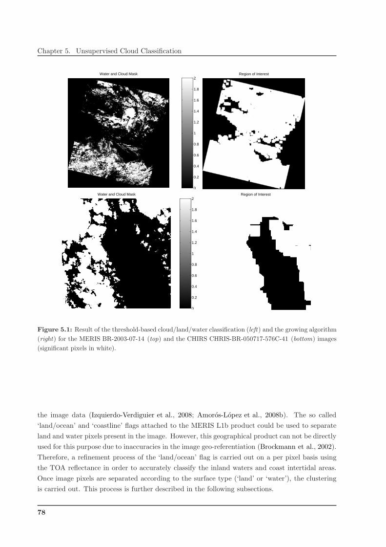
Chapter 5. Unsupervised Cloud Classification
Water and Cloud Mask
0
0.2
0.4
0.6
0.8
1
1.2
1.4
1.6
1.8
2Region of Interest
Water and Cloud Mask
0
0.2
0.4
0.6
0.8
1
1.2
1.4
1.6
1.8
2Region of Interest
Figure 5.1: Result of the threshold-based cloud/land/water classification (left) and the growing algorithm
(right) for the MERIS BR-2003-07-14 (top) and the CHIRS CHRIS-BR-050717-576C-41 (bottom) images
(significant pixels in white).
the image data (Izquierdo-Verdiguier et al., 2008; Amoros-Lopez et al., 2008b). The so called
‘land/ocean’ and ‘coastline’ flags attached to the MERIS L1b product could be used to separate
land and water pixels present in the image. However, this geographical product can not be directly
used for this purpose due to inaccuracies in the image geo-referentiation (Brockmann et al., 2002).
Therefore, a refinement process of the ‘land/ocean’ flag is carried out on a per pixel basis using
the TOA reflectance in order to accurately classify the inland waters and coast intertidal areas.
Once image pixels are separated according to the surface type (‘land’ or ‘water’), the clustering
is carried out. This process is further described in the following subsections.
78
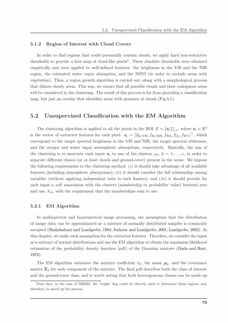
5.2. Unsupervised Classification with the EM Algorithm
5.1.2 Region of Interest with Cloud Covers
In order to find regions that could potentially contain clouds, we apply hard non-restrictive
thresholds to provide a first map of cloud-like pixels1. These absolute thresholds were obtained
empirically and were applied to well-defined features: the brightness in the VIS and the NIR
region, the estimated water vapor absorption, and the NDVI (in order to exclude areas with
vegetation). Then, a region growth algorithm is carried out, along with a morphological process
that dilates cloudy areas. This way, we ensure that all possible clouds and their contiguous areas
will be considered in the clustering. The result of this process is far from providing a classification
map, but just an overlay that identifies areas with presence of clouds (Fig.5.1).
5.2 Unsupervised Classification with the EM Algorithm
The clustering algorithm is applied to all the pixels in the ROI X = {xi}ni=1, where xi ∈ R
d
is the vector of extracted features for each pixel: xi = [fBr,VIS, fBr,NIR, fWh, fO2, fWV]⊤, which
correspond to the target spectral brightness in the VIS and NIR, the target spectral whiteness,
and the oxygen and water vapor atmospheric absorptions, respectively. Basically, the aim of
the clustering is to associate each input xi to one of the clusters ωk, k = 1, . . . , c, in order to
separate different classes (or at least clouds and ground-cover) present in the scene. We impose
the following requirements to the clustering method: (i) it should take advantage of all available
features (including atmospheric absorptions); (ii) it should consider the full relationship among
variables (without applying independent tests to each feature); and (iii) it should provide for
each input a soft association with the clusters (membership or probability value) between zero
and one, hik, with the requirement that the memberships sum to one.
5.2.1 EM Algorithm
In multispectral and hyperspectral image processing, the assumption that the distribution
of image data can be approximated as a mixture of normally distributed samples is commonly
accepted (Shahshahani and Landgrebe, 1994; Jackson and Landgrebe, 2001; Landgrebe, 2002). In
this chapter, we make such assumption for the extracted features. Therefore, we consider the input
as a mixture of normal distributions and use the EM algorithm to obtain the maximum likelihood
estimation of the probability density function (pdf) of the Gaussian mixture (Duda and Hart,
1973).
The EM algorithm estimates the mixture coefficient πk, the mean µk, and the covariance
matrix Σk for each component of the mixture. The final pdf describes both the class of interest
and the ground-cover class, and is worth noting that both heterogeneous classes can be made up
1Note that, in the case of MERIS, the ‘bright’ flag could be directly used to determine these regions and,
therefore, to speed up the process.
79

Chapter 5. Unsupervised Cloud Classification
of more than one mode, each representing a different subclass.
In a mixture model, the probability density function is given by (Duda and Hart, 1973):
p(x|Θ) =
c∑
k=1
p(x|ωk,Θ)P (ωk) (5.2.1)
where ωk are the components, P (ωk) are their prior probabilities, or mixing parameters, and
p(x|ωk,Θ) are the conditional pdf associated to the kth component, being Θ the vector of param-
eters. Sometimes Θ also includes P (ωk). The log likelihood of the independently and identically
distributed (i.i.d.) sample X is:
L(Θ|X ) =∑
i
log p(xi|Θ) =∑
i
log∑
k
p(xi|ωk,Θ)P (ωk) (5.2.2)
This has not a straightforward solution, but the mixture parameters can be estimated using the
EM algorithm, which involves two consecutive iterative steps.
In the E-step, we compute the posteriors as follows:
P (ωk|xi,Θ) =p(xi|ωk,Θ)P (ωk)∑
l p(xi|ωl,Θ)P (ωl)(5.2.3)
which will be also referred to as hik hereafter for the shake of simplicity in the notation. If the
component densities are taken to be d-variate Gaussian, p(x|ωk,Θ) ∼ Nd(µk,Σk):
p(x|ωk,Θ) =1
(2π)d/2|Σk|1/2exp
(
−1
2(x− µk)
⊤Σ−1k (x − µk)
)
(5.2.4)
then we have
hik =πk|Σk|−1/2 exp
(
−(1/2)(xi − µk)⊤Σ−1
k (xi − µk))
∑
l πl|Σl|−1/2 exp(
−(1/2)(xi − µl)⊤Σ−1
l (xi − µl)) (5.2.5)
where we re-define πk ≡ P (ωk).
In the M-step, we update the component parameters Θ:
µk =
∑
i hikxi∑
i hik
Σk =
∑
i hik(xi − µk)(xi − µk)⊤
∑
i hik(5.2.6)
πk =1
n
∑
i
hik
EM initialization
The EM algorithm has to be started with a set of initial values for the parameters of the pdf.
In this work, the k-means algorithm is used to obtain a first approach to the structure of the data
in clusters. This algorithm only needs the number of clusters c to be fixed, and minimizes the
80
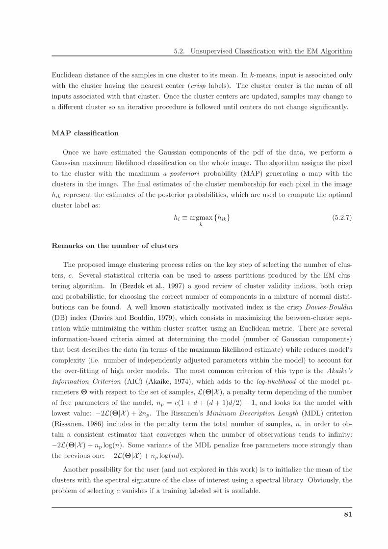
5.2. Unsupervised Classification with the EM Algorithm
Euclidean distance of the samples in one cluster to its mean. In k-means, input is associated only
with the cluster having the nearest center (crisp labels). The cluster center is the mean of all
inputs associated with that cluster. Once the cluster centers are updated, samples may change to
a different cluster so an iterative procedure is followed until centers do not change significantly.
MAP classification
Once we have estimated the Gaussian components of the pdf of the data, we perform a
Gaussian maximum likelihood classification on the whole image. The algorithm assigns the pixel
to the cluster with the maximum a posteriori probability (MAP) generating a map with the
clusters in the image. The final estimates of the cluster membership for each pixel in the image
hik represent the estimates of the posterior probabilities, which are used to compute the optimal
cluster label as:
hi ≡ argmaxk
{hik} (5.2.7)
Remarks on the number of clusters
The proposed image clustering process relies on the key step of selecting the number of clus-
ters, c. Several statistical criteria can be used to assess partitions produced by the EM clus-
tering algorithm. In (Bezdek et al., 1997) a good review of cluster validity indices, both crisp
and probabilistic, for choosing the correct number of components in a mixture of normal distri-
butions can be found. A well known statistically motivated index is the crisp Davies-Bouldin
(DB) index (Davies and Bouldin, 1979), which consists in maximizing the between-cluster sepa-
ration while minimizing the within-cluster scatter using an Euclidean metric. There are several
information-based criteria aimed at determining the model (number of Gaussian components)
that best describes the data (in terms of the maximum likelihood estimate) while reduces model’s
complexity (i.e. number of independently adjusted parameters within the model) to account for
the over-fitting of high order models. The most common criterion of this type is the Akaike’s
Information Criterion (AIC) (Akaike, 1974), which adds to the log-likelihood of the model pa-
rameters Θ with respect to the set of samples, L(Θ|X ), a penalty term depending of the number
of free parameters of the model, np = c(1 + d + (d + 1)d/2) − 1, and looks for the model with
lowest value: −2L(Θ|X ) + 2np. The Rissanen’s Minimum Description Length (MDL) criterion
(Rissanen, 1986) includes in the penalty term the total number of samples, n, in order to ob-
tain a consistent estimator that converges when the number of observations tends to infinity:
−2L(Θ|X ) + np log(n). Some variants of the MDL penalize free parameters more strongly than
the previous one: −2L(Θ|X ) + np log(nd).
Another possibility for the user (and not explored in this work) is to initialize the mean of the
clusters with the spectral signature of the class of interest using a spectral library. Obviously, the
problem of selecting c vanishes if a training labeled set is available.
81
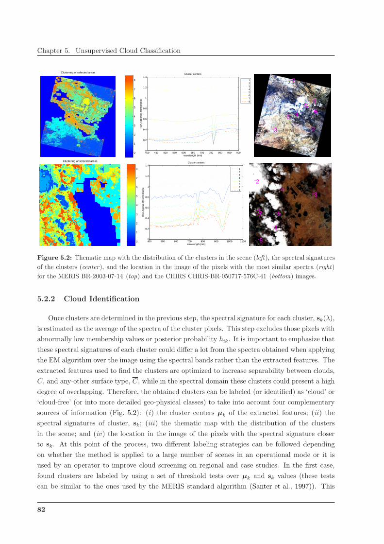
Chapter 5. Unsupervised Cloud Classification
Clustering of selected areas
0
1
2
3
4
5
6
7
8
400 450 500 550 600 650 700 750 800 850 9000
0.2
0.4
0.6
0.8
1
1.2
1.4Cluster centers
wavelength (nm)
TO
A A
ppar
ent R
efle
ctan
ce
12345678 1
23
45
6
7
8
Clustering of selected areas
0
1
2
3
4
5
6
7
8
400 500 600 700 800 900 1000 11000
0.2
0.4
0.6
0.8
1
1.2
1.4Cluster centers
wavelength (nm)
TO
A A
ppar
ent R
efle
ctan
ce
12345678
1
2
34
5 67
8
Figure 5.2: Thematic map with the distribution of the clusters in the scene (left), the spectral signatures
of the clusters (center), and the location in the image of the pixels with the most similar spectra (right)
for the MERIS BR-2003-07-14 (top) and the CHIRS CHRIS-BR-050717-576C-41 (bottom) images.
5.2.2 Cloud Identification
Once clusters are determined in the previous step, the spectral signature for each cluster, sk(λ),
is estimated as the average of the spectra of the cluster pixels. This step excludes those pixels with
abnormally low membership values or posterior probability hik. It is important to emphasize that
these spectral signatures of each cluster could differ a lot from the spectra obtained when applying
the EM algorithm over the image using the spectral bands rather than the extracted features. The
extracted features used to find the clusters are optimized to increase separability between clouds,
C, and any-other surface type, C, while in the spectral domain these clusters could present a high
degree of overlapping. Therefore, the obtained clusters can be labeled (or identified) as ‘cloud’ or
‘cloud-free’ (or into more detailed geo-physical classes) to take into account four complementary
sources of information (Fig. 5.2): (i) the cluster centers µk of the extracted features; (ii) the
spectral signatures of cluster, sk; (iii) the thematic map with the distribution of the clusters
in the scene; and (iv) the location in the image of the pixels with the spectral signature closer
to sk. At this point of the process, two different labeling strategies can be followed depending
on whether the method is applied to a large number of scenes in an operational mode or it is
used by an operator to improve cloud screening on regional and case studies. In the first case,
found clusters are labeled by using a set of threshold tests over µk and sk values (these tests
can be similar to the ones used by the MERIS standard algorithm (Santer et al., 1997)). This
82

5.2. Unsupervised Classification with the EM Algorithm
Classification of selected areas
0:background
1:soil
2:cirrus
3:soil
4:soil
5:clouds
6:bright clouds
7:soil
8:soil
Cloud Probability
0
0.1
0.2
0.3
0.4
0.5
0.6
0.7
0.8
0.9
1
Classification of selected areas
0:background
1:bright clouds
2:bright clouds
3:soil
4:bright clouds
5:cirrus
6:clouds
7:vegetation
8:shadows
Cloud Probability
0
0.1
0.2
0.3
0.4
0.5
0.6
0.7
0.8
0.9
1
Figure 5.3: Thematic map with the distribution in the scene of the classes of the clusters (left) and Cloud
Probability index computed from the posteriors of the cloud-clusters (right) for the MERIS BR-2003-07-14
(top) and the CHIRS CHRIS-BR-050717-576C-41 (bottom) images.
cluster-based approach provides a more accurate cloud screening than the standard approach
(applied on a per pixel basis) since classifying the centers of the clusters should be easier than
classifying single pixels, e.g. pixels close to the decision boundaries. It is worth noting that, in
this case, different classification criteria can be used for clusters found over ‘land’ and over ‘water’.
For regional and case studies, the cluster information can be analyzed directly by the user for
the given image. This can help significantly to identify clusters corresponding to extremely thin
clouds or ice/snow covers misclassified by the automatic labeling. In the following processing steps
of the method, both ‘land’ and ‘water’ clusters are used together to obtain the final probability
and abundance fraction of clouds for all image pixels, and thus obtaining a cloud product map
without discontinuities between land and water.
Once all clusters have been related to a class with a geo-physical meaning (Fig. 5.3[left ]), it
is straightforward to merge all the clusters belonging to a cloud type. Since the EM algorithm
provides posterior probabilities (hik ∈ [0, 1] and∑c
k=1 hik = 1), a probabilistic cloud index, based
on the clustering of the extracted features, can be computed as the sum of the posteriors of the
83

Chapter 5. Unsupervised Cloud Classification
cloud-clusters C:
hiC =∑
ωk⊂C
hik (5.2.8)
However, if the clusters are well separated in the input space, the posteriors decrease drastically
from one to zero in the boundaries between clusters (Fig. 5.3[right ]). Therefore, this Cloud
Probability index indicates the probability that one pixel more likely belongs to a cloud-cluster,
C, than to one of the other clusters, C, found in the image, but it does not give information
about the cloud content at subpixel level, which is very important when dealing with thin clouds
or partially covered pixels.
5.3 Cloud Abundance
In order to obtain a cloud abundance map for every pixel in the image, instead of flags
or a binary classification, a spectral unmixing algorithm is applied to the MERIS image. The
linear spectral unmixing algorithm (LSU) (Chang, 2003) allows decomposing each pixel of the
image, ρi(λ), into a collection of constituent spectra or endmembers, and a set of corresponding
abundances that indicate the proportion of each endmember in the pixel.
5.3.1 Linear Spectral Unmixing
The algorithm used to perform the spectral unmixing is the Fully Constrained Linear Spectral
Unmixing (FCLSU) (Heinz and Chang, 2001; Chang, 2003), which guarantees a physical (yet
linear) interpretation of the results and can be formalized as follows:
ρi(λb) =
Q∑
q=1
mq(λb)aiq + εb (5.3.1)
subject to
0 ≤ aiq ≤ 1 and∑
q
aiq = 1 (5.3.2)
where ρi(λb) is the value of the pixel i for band b; Q represents the number of endmembers that
are being unmixed; and coefficients aiq are the unmixing coefficients, which can be interpreted
as the abundance fractions of materials in a pixel. Finally, the term εb represents the residual
error per band. Equation (5.3.1) can be expressed in a matrix form as ρi = M · ai + ε, where
the spectral signatures of materials, mq, are expressed as the columns of matrix M. The FCLSU
algorithm solves a constrained linear least-squares problem:
minai
‖M · ai − ρi‖ (5.3.3)
subject to (5.3.2), i.e. the vector ai of independent variables is restricted to being nonnegative and
sum to one. This is because ai represents the contribution of reflectance signatures mq and it is
84
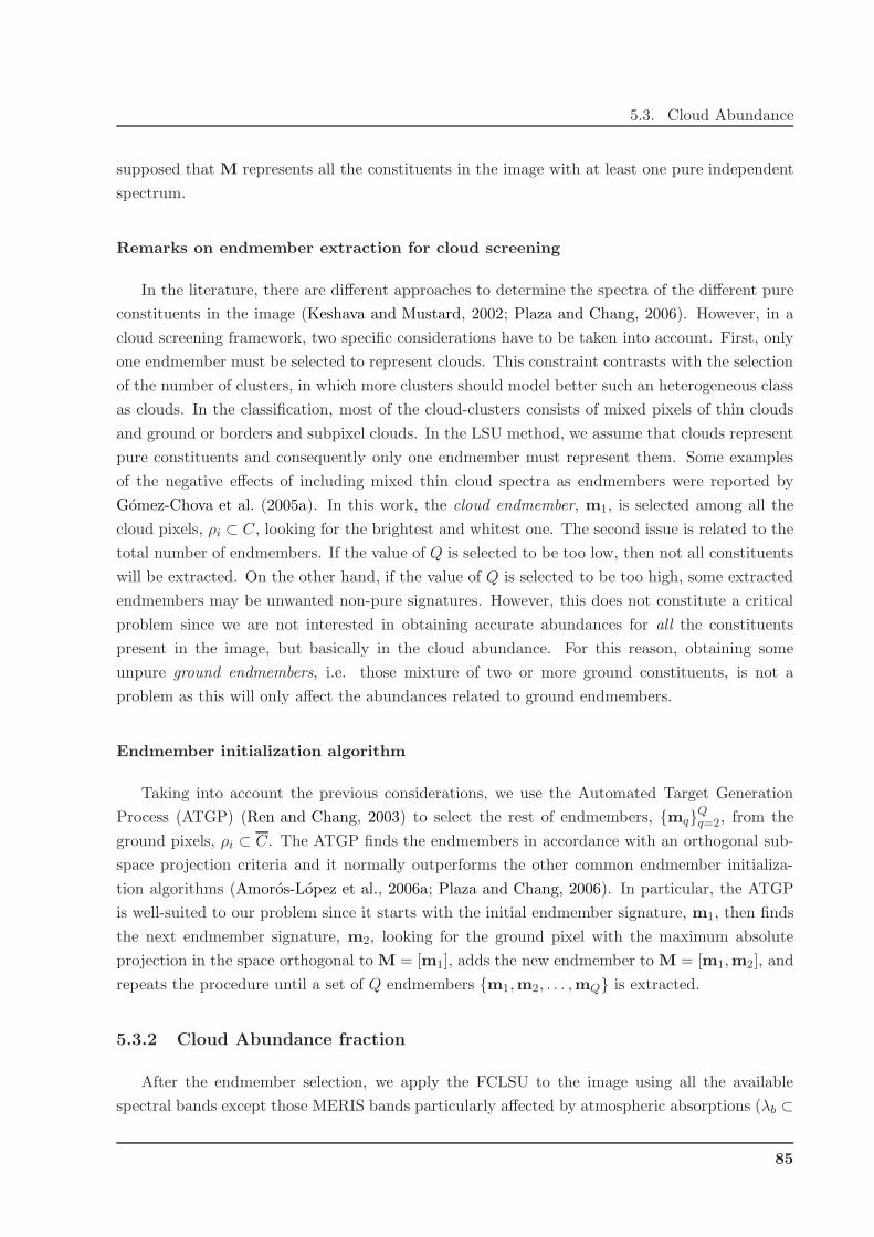
5.3. Cloud Abundance
supposed that M represents all the constituents in the image with at least one pure independent
spectrum.
Remarks on endmember extraction for cloud screening
In the literature, there are different approaches to determine the spectra of the different pure
constituents in the image (Keshava and Mustard, 2002; Plaza and Chang, 2006). However, in a
cloud screening framework, two specific considerations have to be taken into account. First, only
one endmember must be selected to represent clouds. This constraint contrasts with the selection
of the number of clusters, in which more clusters should model better such an heterogeneous class
as clouds. In the classification, most of the cloud-clusters consists of mixed pixels of thin clouds
and ground or borders and subpixel clouds. In the LSU method, we assume that clouds represent
pure constituents and consequently only one endmember must represent them. Some examples
of the negative effects of including mixed thin cloud spectra as endmembers were reported by
Gomez-Chova et al. (2005a). In this work, the cloud endmember, m1, is selected among all the
cloud pixels, ρi ⊂ C, looking for the brightest and whitest one. The second issue is related to the
total number of endmembers. If the value of Q is selected to be too low, then not all constituents
will be extracted. On the other hand, if the value of Q is selected to be too high, some extracted
endmembers may be unwanted non-pure signatures. However, this does not constitute a critical
problem since we are not interested in obtaining accurate abundances for all the constituents
present in the image, but basically in the cloud abundance. For this reason, obtaining some
unpure ground endmembers, i.e. those mixture of two or more ground constituents, is not a
problem as this will only affect the abundances related to ground endmembers.
Endmember initialization algorithm
Taking into account the previous considerations, we use the Automated Target Generation
Process (ATGP) (Ren and Chang, 2003) to select the rest of endmembers, {mq}Qq=2, from the
ground pixels, ρi ⊂ C. The ATGP finds the endmembers in accordance with an orthogonal sub-
space projection criteria and it normally outperforms the other common endmember initializa-
tion algorithms (Amoros-Lopez et al., 2006a; Plaza and Chang, 2006). In particular, the ATGP
is well-suited to our problem since it starts with the initial endmember signature, m1, then finds
the next endmember signature, m2, looking for the ground pixel with the maximum absolute
projection in the space orthogonal to M = [m1], adds the new endmember to M = [m1,m2], and
repeats the procedure until a set of Q endmembers {m1,m2, . . . ,mQ} is extracted.
5.3.2 Cloud Abundance fraction
After the endmember selection, we apply the FCLSU to the image using all the available
spectral bands except those MERIS bands particularly affected by atmospheric absorptions (λb ⊂
85
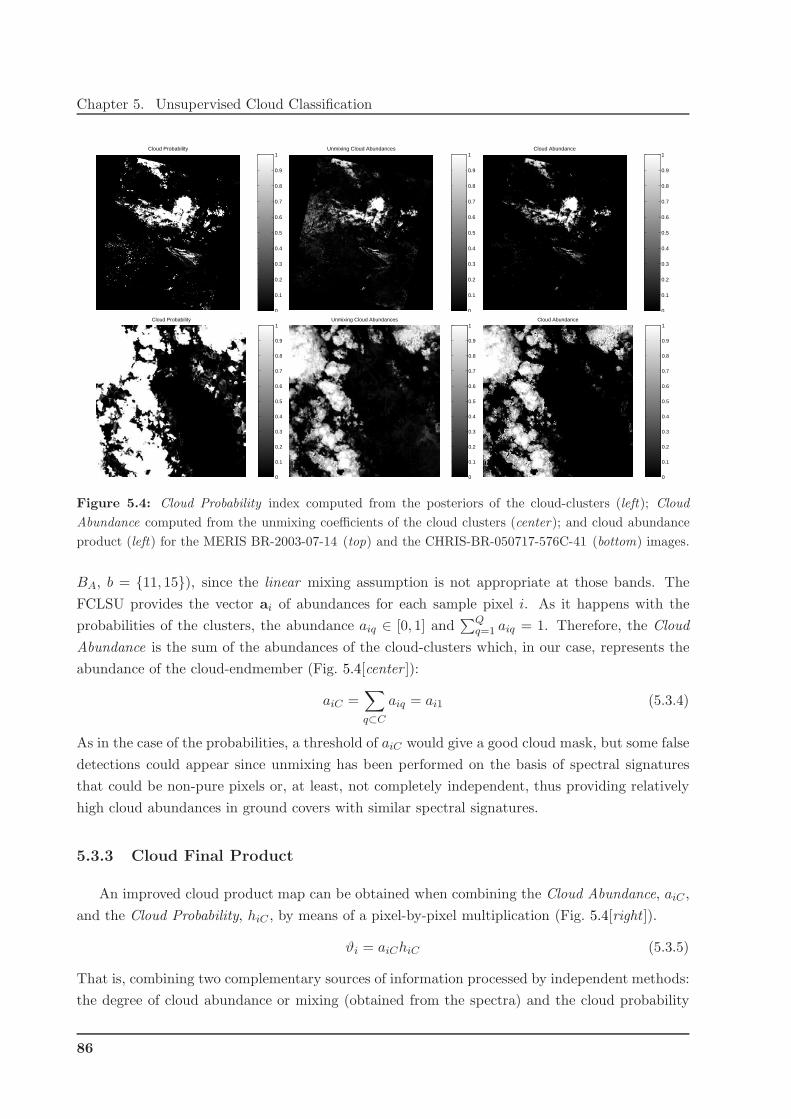
Chapter 5. Unsupervised Cloud Classification
Cloud Probability
0
0.1
0.2
0.3
0.4
0.5
0.6
0.7
0.8
0.9
1Unmixing Cloud Abundances
0
0.1
0.2
0.3
0.4
0.5
0.6
0.7
0.8
0.9
1Cloud Abundance
0
0.1
0.2
0.3
0.4
0.5
0.6
0.7
0.8
0.9
1
Cloud Probability
0
0.1
0.2
0.3
0.4
0.5
0.6
0.7
0.8
0.9
1Unmixing Cloud Abundances
0
0.1
0.2
0.3
0.4
0.5
0.6
0.7
0.8
0.9
1Cloud Abundance
0
0.1
0.2
0.3
0.4
0.5
0.6
0.7
0.8
0.9
1
Figure 5.4: Cloud Probability index computed from the posteriors of the cloud-clusters (left); Cloud
Abundance computed from the unmixing coefficients of the cloud clusters (center); and cloud abundance
product (left) for the MERIS BR-2003-07-14 (top) and the CHRIS-BR-050717-576C-41 (bottom) images.
BA, b = {11, 15}), since the linear mixing assumption is not appropriate at those bands. The
FCLSU provides the vector ai of abundances for each sample pixel i. As it happens with the
probabilities of the clusters, the abundance aiq ∈ [0, 1] and∑Q
q=1 aiq = 1. Therefore, the Cloud
Abundance is the sum of the abundances of the cloud-clusters which, in our case, represents the
abundance of the cloud-endmember (Fig. 5.4[center ]):
aiC =∑
q⊂C
aiq = ai1 (5.3.4)
As in the case of the probabilities, a threshold of aiC would give a good cloud mask, but some false
detections could appear since unmixing has been performed on the basis of spectral signatures
that could be non-pure pixels or, at least, not completely independent, thus providing relatively
high cloud abundances in ground covers with similar spectral signatures.
5.3.3 Cloud Final Product
An improved cloud product map can be obtained when combining the Cloud Abundance, aiC ,
and the Cloud Probability, hiC , by means of a pixel-by-pixel multiplication (Fig. 5.4[right ]).
ϑi = aiChiC (5.3.5)
That is, combining two complementary sources of information processed by independent methods:
the degree of cloud abundance or mixing (obtained from the spectra) and the cloud probability
86

5.3. Cloud Abundance
that is close to one in the cloud-like pixels and close to zero in remaining areas (obtained from
the extracted features). Note that, by performing a pixel-by-pixel multiplication, errors in the
sub-pixel cloud abundance would lead to similar errors in the cloud abundance product. For
example, if an endmember is selected from a ground cover with similar reflectance signature to
the cloud endmember, it could introduce significant errors in the estimated cloud abundance.
However, the endmember selection performed by the ATGP algorithm reduces to some extent the
risk of selecting such spectra. In addition, besides abundance fractions, the unmixing algorithm
provides the unmixing residual error, ε, which informs us about the accuracy of the unmixing on
a per-pixel basis.
87

Chapter 5. Unsupervised Cloud Classification
88

Chapter 6
Semi-supervised Cloud Classification
Applying unsupervised clustering methods over the whole image allows us to take advantage
of the wealth of information and the high degree of spatial and spectral correlation of the image
pixels. However, the cluster labeling strategy presented in the previous chapter (cf. section 5.2.2)
is conceived for scenarios where there is an operator to improve cloud screening on regional and
case studies, but it is not practical when applied to a large number of scenes in an operational
mode. This solution is mostly image oriented and concerned with obtaining more accurate cloud
masks than the standard approach (applied on a per pixel basis), which underperforms in some
critical problems, such as cloud borders and bright surfaces.
When the aim is to process a large number of scenes in an automatic way, we should turn to
robust supervised methods, which learn from a reliable set of labeled training samples in order to
define a decision function that correctly classifies cloudy pixels. However, few labeled samples are
typically available or likely to be obtained in an operational basis. Our aim is to take advantage
of the benefits shown by both supervised and unsupervised methods. For this reason, in this
chapter, we explore the opportunities offered by semi-supervised learning (SSL) that exploits the
few labeled samples and the wealth of unlabeled samples in the images.
In remote sensing image classification, we are usually given a reduced set of labeled samples to
develop the classifier. Learning in these conditions is more challenging when dealing with ill-posed
problems, i.e. working with less labeled samples than the input dimension of the pixels. Super-
vised support vector machines (SVMs) (Scholkopf and Smola, 2001; Camps-Valls et al., 2007c)
excel in using the labeled information, since they are (regularized) maximum margin classifiers also
equipped with an appropriate loss function (Vapnik, 1998; Shawe-Taylor and Cristianini, 2004;
Camps-Valls and Bruzzone, 2005). These methods, nevertheless, need to be reformulated in order
to exploit the information contained in the wealth of unlabeled samples, a.k.a. semi-supervised
classification. In semi-supervised learning, the algorithm is provided with some available super-
vised information in addition to the unlabeled data.
Cloud screening constitutes a clear example of these situations, since few labeled cloud pixels
Chapter 6. Semi-supervised Cloud Classification
are typically available, and cloud features change to a great extent depending on the cloud type,
thickness, transparency, height, or background, as shown in previous chapters. In addition, cloud
screening must be carried out before atmospheric correction, being the input data affected by the
variable atmospheric conditions.
Semi-supervised Learning Framework When working with semi-supervised methods, the
number of reliable labeled samples is usually small and semi-supervised learning methods try
to use the large amount of available unlabeled data by making some assumptions. Only if the
imposed model assumption meets the problem structure, it is possible to learn from unlabeled
samples and to improve classifier performance. The main assumptions made in SSL are the
following:
• The cluster assumption can be roughly stated as “If samples are in the same cluster, they
are likely to belong to the same class”. Nearby points are likely to have the same label
(local consistency), while points on the same data structure are likely to have the same
label (global consistency).
• The manifold1 (smoothness) assumption can be stated as “If two samples in a high-density
region are close, then so should be the corresponding outputs”. If two points are linked by
a path of high density then their outputs are likely to be close (global consistency), but the
contrary is not necessarily true.
The framework of semi-supervised learning is very active and has recently attracted a consid-
erable amount of research (Zhu, 2005; Chapelle et al., 2006). Essentially, two different classes of
SSL algorithms are encountered in the literature.
1. Generative models involve estimating the conditional distribution by means of modeling the
class-conditional distributions explicitly, such as expectation-maximization (EM) algorithms
with finite mixture models (Dempster et al., 1977), which have been extensively applied
in the context of remotely sensed image classification (Shahshahani and Landgrebe, 1994;
Jackson and Landgrebe, 2001; Gomez-Chova et al., 2002, 2003b).
2. Discriminative models estimate the conditional distribution directly and there is no need to
explicitly specify the class-conditional distributions. Two subgroups of SSL algorithms can
be distinguish within these models:
• Low density separation algorithms maximize the margin for labeled and unlabeled sam-
ples simultaneously, such as Transductive SVM (TSVM) (Vapnik, 1998), which has
been recently applied to hyperspectral image classification (Bruzzone et al., 2006);
1A manifold is a topological space that is locally Euclidean, but in which the global structure may be more
complex. Formally, in a “d-dimensional topological manifold” M, for each point x in the manifold M there is an
open subset S with x ∈ S, for which there exists a homeomorphic mapping g that maps S into a d-dimensional
open subset S′ in a d-dimensional Euclidean space Rd (Bachmann et al., 2005, 2006).
90

6.1. Introduction to Kernel Methods
• Graph-based methods, in which each sample spreads its label information to its neigh-
bors until a stable state is achieved on the whole dataset (Chung, 1997) also adapted
to remote sensing image classification by Camps-Valls et al. (2007a).
In the recent years, TSVM and graph-based methods have captured great attention. How-
ever, some specific problems are identified in both of them. In particular, the TSVM is
sensitive to local minima and requires convergence heuristics by using an (unknown) number
of unlabeled samples. Graph-based methods are computationally demanding and generally
do not yield a final decision function but only prediction labels.
In the following sections, we first provide an introduction to kernel-based methods, which have
been selected as the core of the semi-supervised classification algorithms proposed in this Thesis.
Then, we describe a semi-supervised discriminative algorithm based on the graph Laplacian and
SVMs that we propose for its use in cloud screening. Finally, a novel semi-supervised algorithm
based on composite kernels and kernel mean mappings is presented and analyzed in detail.
6.1 Introduction to Kernel Methods
In this section, we first state the general problem of learning from samples, the need of introduc-
ing regularization in the classifiers, and the important concept of kernel feature space. After this,
the formulation and characteristics of each kernel-based method are briefly reviewed. For a full the-
oretical description of these (and other) kernel-based methods, the reader is referred to Scholkopf
(1997); Muller et al. (2001) and for the analysis of hyperspectral image classification with ker-
nels to Camps-Valls et al. (2003, 2004b); Camps-Valls and Bruzzone (2004); Camps-Valls et al.
(2004a); Camps-Valls and Bruzzone (2005); Camps-Valls et al. (2006a); Bruzzone et al. (2007).
6.1.1 Learning from Samples, Regularization, and Kernel feature space
Let us consider a two-class problem, where a labeled training data set {(x1, y1), . . ., (xn, yn)},being xi ∈ R
d and yi ∈ {−1, +1}, is generated according to an (unknown) probability distribution
p(x, y). The problem is to find a function f that minimizes the expected error (or risk)
R(f) =
∫
V (f(x), y)dp(x, y) (6.1.1)
where V represents a pre-defined cost (or loss) function of the errors committed by f . Since the
risk cannot be minimized directly, one follows an inductive principle. A common one consists
in approximating the minimum of the risk by the empirical risk Remp(f), i.e. the error in the
training data set:
Remp(f) =1
n
n∑
i=1
V (f(xi), yi) (6.1.2)
91
Chapter 6. Semi-supervised Cloud Classification
However, convergence of the empirical risk to the actual risk is only ensured as n goes to infinity
and, since this is not possible in real applications, the well-known problem of overfitting may arise.
This is specially significant in hyperspectral image classification given the low ratio between the
number of training samples and the size of the input feature space, and the high spatial variability
of the spectral signature.
In order to control the capacity (or excess of flexibility) of the models and to avoid overfitting,
the solution is usually regularized (Tikhonov and Arsenin, 1977), which is carried out in practice
by minimizing an l-norm of the decision function given by the model parameters, ‖w‖l, in the
corresponding feature space where the function is defined. This is intuitively equivalent to find
the estimator which uses the minimum possible energy of the data to estimate the output, i.e.
by minimizing this term one forces smooth solutions by using small weights, which reduces the
tendency of the model to overfit the training data. The resulting functional should take into
account both this complexity term and an empirical error measurement term defined according to
an a priori determined cost function V of the committed errors. Hence, the regularized minimizing
functional can be written as
Rreg(f) = Remp(f) + γ‖w‖2l , (6.1.3)
where the parameter γ tunes the trade-off between model complexity and minimization of training
errors. It is worth noting that different loss functions V and norms can be adopted for solving
the problem, involving completely different families of models and solutions.
The problem of minimizing the regularized functional in (6.1.3) can be solved following dif-
ferent minimization procedures. Neural networks are trained to minimize the empirical risk, and
therefore, they follow the empirical risk minimization (ERM) principle (Soria-Olivas et al., 2003).
However, on the one hand, in order to attain significant results on the test set, early-stopping
criteria or pruning techniques must be used (Haykin, 1999; Camps-Valls et al., 2006e). On the
other hand, the structural risk minimization (SRM) principle (Vapnik, 1998) states that a better
solution in terms of generalization capabilities can be found by minimizing an upper bound of the
generalization error.
Statistical learning theory points out that learning can be simpler using low complexity clas-
sifiers in high dimension (possibly infinite) spaces H instead of working in the original input
space Rd, i.e. not the dimensionality but the complexity of the function class, which maps in-
put data into H, matters (Vapnik, 2000). Thus, all the potential and richness that a classifier
needs can be introduced by a mapping φ to a Hilbert space H. For instance, in a Radial Ba-
sis Function Neural Network (RBFNN), the Hilbert space H is spanned by the RBF centers,
whereas in the case of SVMs it is expanded by the training samples (Camps-Valls et al., 2004c;
Camps-Valls and Bruzzone, 2005). It is worth noting, nevertheless, that in the machine learning
community, one only refers to kernel methods as those that take advantage of the “kernel trick”,
which allows us to work in the mapped kernel space without explicitly knowing the mapping φ,
92

6.1. Introduction to Kernel Methods
w
margin
(a)
w
margin
(b)
−ξw__
ξw__
Figure 6.1: (a) The Optimal Decision Hyperplane (ODH) in a linearly separable problem. Optimal
margin hyperplane is equivalent to minimizing ‖w‖. Only support vectors (gray-squared samples) are
necessary to define the ODH. (b) Linear decision hyperplanes in nonlinearly separable data can be handled
by including slack variables ξi to allow classification errors.
but only the kernel function formed by the dot product of mapping functions. In the following,
we will always refer to the reproducing kernel Hilbert space (RKHS), where the data is mapped,
as the “kernel space”. Further detailed information on this issue can be found in the next subsec-
tions where kernel-based methods are briefly reviewed. Among all the available kernel machines,
we focus on SVMs, which have recently demonstrated superior performance in the context of
hyperspectral image classification (Camps-Valls and Bruzzone, 2004, 2005). For all methods, we
only review the standard binary formulation since cloud screening can be considered a binary
classification problem.
6.1.2 Support Vector Machines
The classification methodology of SVMs attempts to separate samples belonging to different
classes by tracing maximum margin hyperplanes in the kernel space where samples are mapped
to (see Fig. 6.1(a)). Maximizing the distance of samples to the optimal decision hyperplane is
equivalent to minimizing the norm of w, and thus this becomes the first term in the minimizing
functional. For better manipulation of this functional, the quadratic norm of the weights is
preferred. Therefore, following previous notation, the SVM method solves the following primal
problem:
minw,ξi,b
{
1
2‖w‖2 + C
∑
i
ξi
}
(6.1.4)
constrained to:
yi(〈φ(xi),w〉 + b) ≥ 1 − ξi ∀i = 1, . . . , n (6.1.5)
ξi ≥ 0 ∀i = 1, . . . , n (6.1.6)
93

Chapter 6. Semi-supervised Cloud Classification
where w is the normal to the optimal decision hyperplane defined as 〈w,φ(x)〉 + b = 0, and b
represents the bias or closest distance to the origin of the coordinate system. These parameters
define a linear classifier in the kernel space H:
y∗ = f(x∗) = sgn(〈w,φ(x∗)〉 + b) (6.1.7)
The non-linear function φ maps samples to a higher dimensional space, which in accordance
with Cover’s theorem (Cover, 1965), guarantees that the transformed samples are more likely to
be linearly separable. The regularization parameter C controls the generalization capabilities of
the classifier, and ξi are positive slack variables allowing to deal with permitted errors (see Fig.
6.1(b)).
The above problem is solved by introducing Lagrange multipliers (ξi ≥ 0, µi ≥ 0) for each
constraint:
minw,ξ,b
{
‖w‖2 + Cn∑
i=1
ξi −n∑
i=1
αi[yi(〈w,φ(xi)〉 + b) + ξi − 1] −n∑
i=1
µiξi
}
(6.1.8)
Now, by making zero the gradient of this primal-dual functional Lpd with respect to the primal
variables (w, b, ξi), we obtain the following conditions:
∂Lpd
∂w= 0 → w =
∑
i
yiαiφ(xi) (6.1.9)
∂Lpd
∂b= 0 →
∑
i
yiαi = 0 (6.1.10)
∂Lpd
∂ξi= 0 → C = αi + µi, i = 1, . . . , n (6.1.11)
If constraints (6.1.9)-(6.1.11) are included in the Lagrange functional Lpd (Eq. (6.1.8)) in order
to remove the primal variables, the dual problem Ld to be solved is obtained:
maxα
∑
i
αi −1
2
∑
i,j
αiαjyiyj〈φ(xi),φ(xj)〉
, (6.1.12)
constrained to 0 ≤ αi ≤ C and∑
i αiyi = 0, ∀i = 1, . . . , n. In this way, one gets rid of the
explicit usage of very high dimensional vectors, w. This constitutes a quadratic programming
(QP) problem with linear constraints, and can be solved with many available software packages.
It is worth noting that all φ mappings used in the SVM learning occur in the form of inner
products. This allows us to define a kernel function K:
K(xi,xj) = 〈φ(xi),φ(xj)〉, (6.1.13)
and then, without considering the mapping φ explicitly, a non-linear SVM can be defined. Note
94
6.1. Introduction to Kernel Methods
that the pair {H,φ} will only exist if the kernel function K fullfils Mercer’s conditions2 as will
be detailed in the following section.
After solving the QP problem with a given kernel function, one obtains the optimal Lagrange
multipliers, αi, which reflect the relative relevance of each sample for classification. The key
issue is that we have worked implicitely in the higher dimensional feature space, and retrieve a
weight vector in the original input space. Note that, by solving the optimization problem, the
feature-space model parameters w are expressed as a linear expansion of the mapped samples
φ(xi) through the dual parameters αi, i.e. w =∑n
i=1 yiαiφ(xi) (Eq. (6.1.9)).
By plugging (6.1.9) into (6.1.7), the decision function for any test vector x∗ is given by:
y∗ = f(x∗) = sgn
(
n∑
i=1
yiαiK(xi,x∗) + b
)
, (6.1.14)
where b is calculated using the primal-dual relationship, and where only samples with non-zero
Lagrange multipliers αi account for the solution. This leads to the very important concept of spar-
sity, i.e. the solution is expressed as a function only of the most critical training samples in the
distribution, namely support vectors (SV). For deeper analysis and application of SVMs in RS im-
age classification refer to Gualtieri and Cromp (1998); Gualtieri et al. (1999); Camps-Valls et al.
(2004a); Camps-Valls and Bruzzone (2005).
6.1.3 Composite Kernels Framework
The bottleneck for any kernel method is the definition of a suitable kernel mapping function
that accurately reflects the similarity (distance, resemblance) between samples. However, not
all metric distances are permitted. In fact, valid kernels are only those fulfilling the Mercer’s
Theorem (Mercer, 1905; Aizerman et al., 1964).
Some popular kernels fulfilling these conditions are:
• Linear kernel:
K(xi,xj) = 〈xi,xj〉 (6.1.15)
• Non-homogeneous Polynomial:
K(xi,xj) = (〈xi,xj〉 + 1)p, p ∈ Z+ (6.1.16)
2According to Hilbert-Schmidt theory, K(xi,xj) can be any symmetric function satisfying Mercer’s conditions.
This was firstly stated by Courant and Hilbert (1953). The same idea was used by Aizerman et al. (1964) for the
analysis of the convergence properties of the method of potential functions, and happened at the same time as the
method of the optimal hyperplane was developed by Vapnik and Chervonenkis (1964). Full details on the Mercer’s
conditions can be obtained from Vapnik (2000).
95
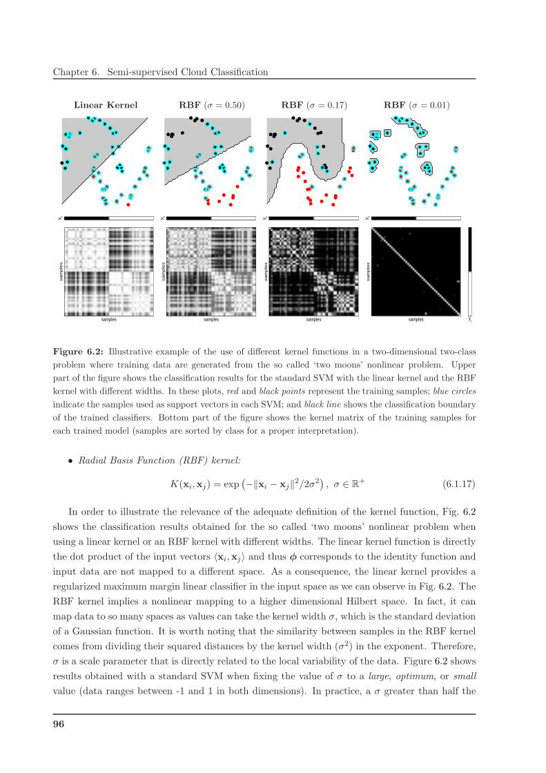
Chapter 6. Semi-supervised Cloud Classification
Linear Kernel RBF (σ = 0.50) RBF (σ = 0.17) RBF (σ = 0.01)
sa
mp
les
samples yi
yi
sa
mp
les
samples yi
yi
sa
mp
les
samples yi
yi
sa
mp
les
samples yi
yi
Figure 6.2: Illustrative example of the use of different kernel functions in a two-dimensional two-class
problem where training data are generated from the so called ‘two moons’ nonlinear problem. Upper
part of the figure shows the classification results for the standard SVM with the linear kernel and the RBF
kernel with different widths. In these plots, red and black points represent the training samples; blue circles
indicate the samples used as support vectors in each SVM; and black line shows the classification boundary
of the trained classifiers. Bottom part of the figure shows the kernel matrix of the training samples for
each trained model (samples are sorted by class for a proper interpretation).
• Radial Basis Function (RBF) kernel:
K(xi,xj) = exp(
−‖xi − xj‖2/2σ2)
, σ ∈ R+ (6.1.17)
In order to illustrate the relevance of the adequate definition of the kernel function, Fig. 6.2
shows the classification results obtained for the so called ‘two moons’ nonlinear problem when
using a linear kernel or an RBF kernel with different widths. The linear kernel function is directly
the dot product of the input vectors 〈xi,xj〉 and thus φ corresponds to the identity function and
input data are not mapped to a different space. As a consequence, the linear kernel provides a
regularized maximum margin linear classifier in the input space as we can observe in Fig. 6.2. The
RBF kernel implies a nonlinear mapping to a higher dimensional Hilbert space. In fact, it can
map data to so many spaces as values can take the kernel width σ, which is the standard deviation
of a Gaussian function. It is worth noting that the similarity between samples in the RBF kernel
comes from dividing their squared distances by the kernel width (σ2) in the exponent. Therefore,
σ is a scale parameter that is directly related to the local variability of the data. Figure 6.2 shows
results obtained with a standard SVM when fixing the value of σ to a large, optimum, or small
value (data ranges between -1 and 1 in both dimensions). In practice, a σ greater than half the
96

6.1. Introduction to Kernel Methods
maximum Euclidean distance between all samples will provide results similar to the linear kernel
since a high value (σ = 0.5) would imply low variability or local structure. On the other hand, a σ
smaller than half the smallest Euclidean distance between training samples would make samples
go too far from each other (with respect to the Gaussian) to extract the structure of data. This is
shown for σ = 0.01, where the imposed data locality leads to overfit 3 training samples. For this
case, classification boundary clearly overfits the training data, all training samples are selected
as support vectors (blue circles), and the kernel matrix is almost diagonal (no class structure is
observed). Finally, the value σ = 0.17 is selected through cross-validation in the training set. In
this case, a nonlinear classifier is obtained while optimizing its generalization capabilities, and the
kernel matrix structure reflects the class information. Summarizing, when using RBF kernels, the
more local data structure is, the smaller σ should be.
In this section, we review the main properties of kernels and the framework of composite
kernels, which will be explained to later present a novel semi-supervised kernel algorithm for
cloud classification.
Properties of Mercer’s kernels
In the context of SVMs in particular and kernel methods in general, one can use any kernel
function K(·, ·) that fullfils Mercer’s condition, which can be stated formally in the following
theorem:
Theorem 1. Mercer’s kernel. Let X be any input space and K: X × X −→ R a symmetric
function, K is a Mercer’s kernel if and only if the kernel matrix formed by restricting K to any
finite subset of X is positive semi-definite, i.e. having no negative eigenvalues.
The Mercer condition constitutes the key requirement to obtain a unique global solution when
developing kernel-based classifiers (e.g. SVMs) since they reduce to solving a convex optimization
problem (Cristianini and Shawe-Taylor, 2000). In addition, important properties for Mercer’s
kernels can be derived from the fact that they are positive-definite (affinity) matrices, as follows:
Property 1. Be K1 and K2 valid Mercer’s kernels over X × X , with xi ∈ X ⊆ Rd, with A being
a symmetric positive semi-definite n× n matrix, and α > 0. Then, the following kernels:
K(xi,xj) = K1(xi,xj) +K2(xi,xj) (6.1.18)
K(xi,xj) = αK1(xi,xj) (6.1.19)
K(xi,xj) = x⊤i Axj (6.1.20)
K(xi,xj) = K1(xi,xj)K2(xi,xj) (6.1.21)
3Overfitting consists in perfectly fitting available data with a false model by increasing its complexity, i.e. its
number of parameters, but reducing the ability of the model to generalize beyond the fitting data. Therefore, it will
not be able to predict the correct output for other examples, thus it will not generalize to situations not presented
during the training process.
97

Chapter 6. Semi-supervised Cloud Classification
are valid Mercer’s kernels. �
Therefore, one can design kernels by summing, weighting, or multiplying dedicated kernels.
This intuitive idea is formally expressed in the following. It is worth noting that the size of
the training kernel matrix is n × n and each position (i, j) of the kernel matrix K contains the
similarity between all possible pairs of training samples measured with a suitable kernel function
K fulfilling Mercer’s conditions. As shown before, some popular kernels are: linear, polynomial,
or radial basis function. This (distance or similarity) matrix is precomputed at the very beginning
of the minimization procedure, and thus, one usually works with the transformed input data, K,
rather than the original input space samples, xi. This fact allows us to easily combine positive
definite kernel matrices taking advantage of the properties in Proposition 1, as will be shown in
the next section.
Composite kernels for hyperspectral image classification
In (Camps-Valls et al., 2006d), we explicitly formulated a full family of kernel-based classifiers
that combine different kernels in order to simultaneously take into account spectral, spatial,
and local cross-information in a hyperspectral image. This framework was further extended in
(Camps-Valls et al., 2008a) to multitemporal and multisource classification and change detection
problems. Basically, we take advantage of two specially interesting properties of kernel methods:
(i) their good performance when working with high input dimensional spaces (Camps-Valls et al.,
2004a; Camps-Valls and Bruzzone, 2005), and (ii) the properties derived from Mercer’s conditions
by which a scaled summation of (positive definite) kernel matrices is a valid kernel, which have
provided good results in other domains (Mak et al., 2004; Sun et al., 2004).
A full family of composite kernels for the combination of different information types is pre-
sented in this section. The following composite kernels are defined for two types of information
only A and B. In any case, the formulations proposed in this section can be easily extended to
any number of information types. For this purpose, three steps are followed:
1. Pixel definition. A pixel entity xi is defined simultaneously in both informative domains A,
xAi ∈ R
dA , and B, xBi ∈ R
dB .
2. Kernel computation. Once that both input vectors xAi and xB
i are constructed, different ker-
nel matrices can be easily computed using any suitable kernel function that fulfills Mercer’s
conditions.
3. Kernel combination. At this point, we take advantage of the direct sum of Hilbert spaces
by which two (or more) Hilbert spaces Hk can combined into a larger Hilbert space, H =
H1 ⊕H2 ⊕ · · · ⊕ HN .
In the following, we present three different kernel approaches for hyperspectral image classification.
98

6.2. Semi-supervised Classification with the Laplacian SVM
The stacked-features approach A good example of the applicability of composite kernels
to remote sensing is the combination of spectral and contextual information of the pixels. The
most commonly adopted approach in hyperspectral image classification is to exploit the spectral
content of a pixel, defined as xAi . However, performance can be improved by including also the
textural information in the classifier, defined as xBi . This is usually done by means of the ‘stacked’
approach, in which feature vectors are built from the concatenation of both types of features. Note
that if the chosen mapping φ is a transformation of the concatenation xi ≡ {xAi , xB
i }, then the
corresponding ‘stacked’ kernel matrix is:
K{A,B} ≡ K(xi,xj) = 〈φ(xi),φ(xj)〉, (6.1.22)
which does not include explicit cross relations between different information features xAi and xB
j .
The direct summation kernel A simple composite kernel combining two types of information
naturally comes from the concatenation of nonlinear transformations of xAi and xB
i . Let us assume
two nonlinear transformations ϕ1(·) and ϕ2(·) into Hilbert spaces H1 and H2, respectively. Then,
the following transformation can be constructed:
φ(xi) = {ϕ1(xAi ), ϕ2(x
Bi )} (6.1.23)
and the corresponding dot product can be easily computed as follows:
K(xi,xj) = 〈φ(xi),φ(xj)〉= 〈{ϕ1(x
Ai ), ϕ2(x
Bi )}, {ϕ1(x
Aj ), ϕ2(x
Bj )}〉 (6.1.24)
= KA(xAi ,x
Aj ) +KB(xB
i ,xBj )
Note that the solution is expressed as the sum of positive definite matrices, with dim(xAi ) = dA,
dim(xBi ) = dB, and dim(K) = dim(KA) = dim(KB) = n× n.
The weighted summation kernel By exploiting Property (2) in Proposition 1, a composite
kernel that balances both information types in (6.1.24) can also be created, as follows:
K(xi,xj) = νKA(xAi ,x
Aj ) + (1 − ν)KB(xB
i ,xBj ) (6.1.25)
where ν is a positive real-valued free parameter (0 < ν < 1), which is tuned in the training process
and constitutes a trade-off between the spatial and spectral information to classify a given pixel.
This composite kernel allows introducing a priori knowledge in the classifier or allows extracting
some information from the best tuned ν parameter.
6.2 Semi-supervised Classification with the Laplacian SVM
In this section, we present a recently introduced semi-supervised framework that incorporates
labeled and unlabeled data in any general-purpose learner (Belkin and Niyogi, 2004; Belkin et al.,
99

Chapter 6. Semi-supervised Cloud Classification
2006). We focus on a semi-supervised extension of the SVM, which introduces an additional reg-
ularization term on the geometry of both labeled and unlabeled samples by using the graph
Laplacian (Chung, 1997), thus leading to the so-called Laplacian SVM (LapSVM) (Belkin et al.,
2006). This methodology follows a non-iterative optimization procedure, in contrast to most
transductive learning methods, and provides a closed-form classification function for testing on
novel samples not used in the training phase (out-of-sample predictions), in contrast to graph-
based approaches. In addition, the Laplacian SVM constitutes a general framework for SSL,
in which supervised SVM and other methods can be regarded just as particular cases. Hard-
margin SVM, directed graph methods, label propagation methods, and spectral clustering solu-
tions (Shawe-Taylor and Cristianini, 2004; Chapelle et al., 2006) are obtained for particular free
parameters of the LapSVM.
The use of the Laplacian SVM algorithm in the field of remote sensing was introduced for the
first time in (Gomez-Chova et al., 2007b) for cloud screening of MERIS data, and was extended
in (Gomez-Chova et al., 2008c) for a urban monitoring application combining multispectral and
SAR data from LANDSAT/TM and ERS (Gomez-Chova et al., 2004b,c, 2006e) or from MERIS
and ASAR (Gomez-Chova et al., 2005d). The reason for using LapSVM is that it permits using
the labeled samples, and efficiently exploiting the information contained in the high number of
available unlabeled pixels to characterize the marginal distribution of data. This is particularly
interesting in practical remote-sensing applications since obtaining additional unlabeled samples
is cheap and easy, while labeling is expensive, difficult, or even impossible.
6.2.1 Manifold Regularization Learning Framework
Regularization is necessary to produce smooth decision functions and thus avoiding overfitting
to the training data. Since the work of Tikhonov (1963), many regularized algorithms have been
proposed to control the capacity of the classifier (Evgeniou et al., 2000; Scholkopf and Smola,
2001). The regularization framework has been recently extended to the use of unlabeled samples
(Belkin et al., 2006) as follows.
Notationally, we are given a set of ℓ labeled samples, {xi, yi}ℓi=1, and a set of u unlabeled
samples {xi}ℓ+ui=ℓ+1, where xi ∈ R
d and yi ∈ {−1,+1}. Let us now assume a general-purpose
decision function f . The regularized functional to be minimized is defined as:
Rreg(f) =1
ℓ
ℓ∑
i=1
V (f(xi), yi) + γL‖f‖2H + γM‖f‖2
M, (6.2.1)
where V represents a generic cost function of the committed errors on the labeled samples, γL
controls the complexity of f in the associated Hilbert space H, and γM controls its complexity
in the intrinsic geometry of the marginal data distribution p(x). For example, if the probability
distribution is supported on a low-dimensional manifold, ‖f‖2M penalizes f along that manifold
M. Note that this functional constitutes a general regularization framework that takes into
account all the available knowledge.
100
6.2. Semi-supervised Classification with the Laplacian SVM
6.2.2 Laplacian Support Vector Machines
The previous semi-supervised learning framework allows us to develop many different algo-
rithms just by playing around with the loss function, V , and the regularizers for the function f .
In this work, we focus on the Laplacian SVM formulation, which basically uses SVM as the core
learner and the graph Laplacian for manifold regularization. In the following, we review all the
ingredients of the formulation.
Cost function of the errors
The Laplacian SVM uses the same hinge loss function as the traditional SVM:
V (f(xi), yi) = max{0, 1 − yif(xi)}, (6.2.2)
where f represents the decision function implemented by the selected classifier and predicted
labels are y∗ = sgn (f(x∗)).
Decision function
We use as the decision function f(x∗) = 〈w,φ(x∗)〉+ b, where φ(·) is a nonlinear mapping to
a higher (possibly infinite) dimensional Hilbert space H, and w and b define a linear regression
in that space. By means of the Representer Theorem (Scholkopf and Smola, 2001), weights w
can be expressed in the dual problem as the expansion over labeled and unlabeled samples w
=∑ℓ+u
i=1 αiφ(xi) = Φα, where Φ = [φ(x1), . . . ,φ(xℓ+u)]⊤ and α = [α1, . . . , αℓ+u]. Then, the
decision function is given by:
f(x∗) =ℓ+u∑
i=1
αiK(xi,x∗) + b, (6.2.3)
and K is the kernel matrix formed by kernel functions K(xi,xj) = 〈φ(xi),φ(xj)〉. The key
point here is that, without considering the mapping φ explicitly, a non-linear classifier can be
constructed by selecting the proper kernel. Also, the regularization term can be fully expressed
in terms of the kernel matrix and the expansion coefficients:
‖f‖2H = ‖w‖2 = (Φα)⊤(Φα) = α⊤Kα. (6.2.4)
Manifold regularization
The geometry of the data is typically modeled with a graph whose nodes represent both
labeled and unlabeled samples connected by weights Wij (Jordan, 1999; Chapelle et al., 2006).
Regularizing the graph follows from the smoothness (or manifold) assumption and intuitively is
101
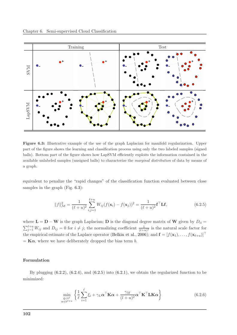
Chapter 6. Semi-supervised Cloud Classification
Training Test
SV
M -
+
-
+
-
+
-
+
Lap
SV
M -
+
-
+
-
+
-
+
Figure 6.3: Illustrative example of the use of the graph Laplacian for manifold regularization. Upper
part of the figure shows the learning and classification process using only the two labeled samples (signed
balls). Bottom part of the figure shows how LapSVM efficiently exploits the information contained in the
available unlabeled samples (unsigned balls) to characterize the marginal distribution of data by means of
a graph.
equivalent to penalize the “rapid changes” of the classification function evaluated between close
samples in the graph (Fig. 6.3):
‖f‖2M =
1
(ℓ+ u)2
ℓ+u∑
i,j=1
Wij(f(xi) − f(xj))2 =
1
(ℓ+ u)2f⊤Lf , (6.2.5)
where L = D− W is the graph Laplacian; D is the diagonal degree matrix of W given by Dii =∑ℓ+u
j=1 Wij and Dij = 0 for i 6= j; the normalizing coefficient 1(ℓ+u)2
is the natural scale factor for
the empirical estimate of the Laplace operator (Belkin et al., 2006); and f = [f(x1), . . . , f(xℓ+u)]⊤
= Kα, where we have deliberately dropped the bias term b.
Formulation
By plugging (6.2.2), (6.2.4), and (6.2.5) into (6.2.1), we obtain the regularized function to be
minimized:
minξ∈Rℓ
α∈Rℓ+u
{
1
ℓ
ℓ∑
i=1
ξi + γLα⊤Kα +γM
(l + u)2α⊤K⊤LKα
}
(6.2.6)
102
6.2. Semi-supervised Classification with the Laplacian SVM
subject to:
yi
( ℓ+u∑
j=1
αjK(xi,xj) + b
)
≥ 1 − ξi, i = 1, . . . , ℓ (6.2.7)
ξi ≥ 0 i = 1, . . . , ℓ (6.2.8)
where ξi are slack variables to deal with committed errors in the labeled samples. Introducing
restrictions (6.2.7)-(6.2.8) into the primal functional (6.2.6) through Lagrange multipliers, βi and
ηi, and taking derivatives w.r.t. b and ξi, we obtain:
minα,β
{
1
2α⊤
(
2γLK +2γM
(ℓ+ u)2K⊤LK
)
α − α⊤KJ⊤Yβ +
ℓ∑
i=1
βi
}
, (6.2.9)
where J = [I 0] is an ℓ × (ℓ + u) matrix with I as the ℓ × ℓ identity matrix (the first ℓ points
are labeled) and Y = diag(y1, . . . , yℓ). Taking derivatives again w.r.t. α, we obtain the solution
(Belkin et al., 2006):
α =
(
2γLI + 2γM
(ℓ+ u)2LK
)−1
J⊤Yβ∗ (6.2.10)
Now, substituting again (6.2.10) into the dual functional (6.2.9), we obtain the following quadratic
programming problem to be solved:
β∗ = maxβ
{ ℓ∑
i=1
βi −1
2β⊤Qβ
}
(6.2.11)
subject to∑ℓ
i=1 βiyi = 0 and 0 ≤ βi ≤ 1ℓ , i = 1, . . . , ℓ, where
Q = YJK
(
2γLI + 2γM
(ℓ+ u)2LK
)−1
J⊤Y (6.2.12)
Therefore, the basic steps for obtaining the weights αi for the solution in (6.2.3) are: (i) build the
weight matrix W and compute the graph Laplacian L = D− W, (ii) compute the kernel matrix
K, (iii) fix regularization parameters γL and γM , and (iv) compute α using (6.2.10) after solving
the problem (6.2.11).
Relation with other classifiers
The Laplacian SVM is intimately related to other unsupervised and semi-supervised classi-
fiers. This is because the method incorporates both the concepts of kernels and graphs in the
same classifier, thus having connections with transduction, clustering, graph-based and label prop-
agation methods. The minimizing functional used in the standard TSVM considers a different
regularization parameter for labeled and unlabeled samples, which is the case in the proposed
framework. Also, LapSVM is directly connected with the soft-margin SVM (γM = 0), the hard
103
Chapter 6. Semi-supervised Cloud Classification
margin SVM (γL → 0, γM = 0), the graph-based regularization method (γL → 0, γM > 0), the
label-propagation regularization method (γL → 0, γM → 0, γM ≫ γL), and spectral clustering
(γM = 1). In conclusion, by optimizing parameters γL and γM over a wide enough range, the
LapSVM theoretically outperforms the aforementioned classifiers. See (Belkin et al., 2006) for
deeper details and theoretical comparison.
6.2.3 Remarks on Laplacian SVM
This method brings together the ideas of spectral graph theory, manifold learning, and kernel-
based algorithms in a coherent and natural way to incorporate geometric structure with a kernel-
based regularization framework. The solution of the LapSVM constitutes a convex optimization
problem and results in a natural out-of-sample extension from the labeled and unlabeled training
samples to novel examples, thus solving the problems of previously proposed methods.
The potential of this classification method in remote sensing image classification increases
when reduced labeled training sets are available. In particular, in cloud screening, it becomes
very difficult to obtain a representative training set for all possible situations, motivating the
introduction of a semi-supervised method exploiting the unlabeled data.
The main problem is related to the computational cost, since a huge matrix consisting of
labeled and unlabeled samples must be inverted (see Eqs. 6.2.10 and 6.2.12). Note, however,
that in this method it is not necessary to incorporate all unlabeled samples in the image so the
computational load is easily scalable. However, smart sampling strategies developed to select
the most informative unlabeled samples could yield improve performance. In this respect, a
modified manifold regularization method for large-scale problems has been recently presented by
Tsang and Kwok (2007).
Another problem when using the Laplacian SVM in cloud screening is that it assumes that
considered problems hold a non-linear manifold. However, distribution of remote sensing data,
and of clouds in particular, can differ to a great extent from a manifold, making the cluster
assumption more suitable in these cases.
6.3 Semi-supervised Classification with Composite Mean Ker-
nels
In previous sections, we introduced kernel-based classification methods and pointed out the
advantages offered by SSL in EO applications. However, SSL approaches make some model
assumptions to improve classification performance by using unlabeled data that do not necessarily
hold in our problem. Consequently, when selecting or developing an SSL method, one has to verify
that the imposed model assumptions meet the problem data structure.
In this section, we propose a semi-supervised kernel-based classification method that takes
104

6.3. Semi-supervised Classification with Composite Mean Kernels
into account the particularities and problems found in practical cloud screening of EO images.
The main issues to be considered before presenting the method can be summarized as follows:
Data Structure. The main assumptions made about data structure in SSL are that data are
organized into a number of groups or clusters according to a given distance measure in some
representation space (cluster assumption) or that data hold a manifold forming a non-linear
complex global structure (manifold assumption) (Bachmann et al., 2005, 2006). In the case
of clouds, and most natural land covers, distribution of remote sensing data is smooth and
spectra of pixels of the same land cover are similar, making the cluster assumption more
suitable to model each class. This is why the proposed method assumes that data are
organized into a number of groups or clusters according to a given distance measure in some
representation space. If the correspondence between sample and cluster is known for some
training samples, one can reinforce samples in the same cluster to belong to the same class
by taking into account the similarity between clusters.
SSL Model. In general, SSL methods aim to retrieve information from unlabeled data by esti-
mating its conditional distribution, and one can distinguish between generative models and
discriminative models to accomplish that. In multispectral image processing, the assumption
that the data distribution can be approximated as a mixture of normally distributed samples
is commonly accepted (Shahshahani and Landgrebe, 1994; Jackson and Landgrebe, 2001).
Hence, generative models, which estimate the conditional distribution by modeling the class-
conditional distributions explicitly, may provide a good performance in cloud screening and
perfectly fit the cluster assumption.
Basic Operations in the Kernel Space. One of the basic ideas when working with kernel
methods is that the mapping φ(x) into the kernel-defined feature space H needs not to be
explicitly known. Although we do not have access to the representation of samples in this
space, it is possible to perform some elementary calculations in the kernel space, such as
computing means and distances.
Training Set Representativeness. In many remote sensing image classification problems, it
is difficult to collect a sufficient number of statistically significant ground-truth samples to
define a complete training set for developing robust supervised classifiers. In this setting, two
main different conditions are usually considered: (1) few training samples are available for
characterizing the image to be classified; and (2) no training samples are available for the test
image to be classified. In the later case, one-class classifiers can be used (Munoz-Marı et al.,
2007, 2008). We instead adopt another strategy by which training data extracted from other
images modeling similar problems can be exploited. In both situations, unlabeled samples
of test image can be jointly used with the available training samples for increasing the
reliability and accuracy of the classifier.
All these issues are addressed in this section. First, some recommendations about how to use
105

Chapter 6. Semi-supervised Cloud Classification
clustering methods to extract information from unlabeled samples of the test image are given.
Then, the concept of mean kernel is introduced to compute cluster similarities and then it is
extended under the framework of composite kernels (Camps-Valls et al., 2006d). Finally, the
proposed solution is presented. It is based on the idea that clouds in the test image present
features that form compact clusters, and unlabeled data coming from similar images can help
to model these clusters and to improve classification performance at pixel level by reinforcing
samples in the same cluster to belong to the same class. Consequently, the aim of the algorithm is
to compute and combine both similarity between samples and similarity between clusters in the
kernel space, while performing the classification at a sample or pixel level. The section closes with
a comprehensive comparison of the benchmarked kernel-based methods with special emphasis on
the pros and cons of the proposed method.
6.3.1 Image Clustering
It is worth noting that the distribution of remote sensing data over natural land covers is
usually smooth and spectra of pixels of the same land cover are locally similar, making the
cluster assumption more suitable in the general case. In this work, clusters of the analyzed
image are found by applying a clustering algorithm, which provides for each sample xi a crisp
or soft association, hik, with each cluster ωk. In particular, we consider the input image as
a mixture of normal distributions so the EM algorithm can be used to obtain the maximum
likelihood estimation of the probability density function (pdf) of the Gaussian mixture. The
EM algorithm estimates the mixture coefficient πk, the mean µk, and the covariance matrix Σk
for each component of the mixture. Then, the algorithm assigns each pixel to the cluster with
the maximum a posteriori probability (MAP); and the cluster membership hik represents the
estimates of the posterior probabilities; that is, membership or probability value between zero
and one, with the requirement that the memberships of one sample to all the clusters sum to one∑
k hik = 1. Hence, the optimal cluster label for each sample is found as hi = argmaxk
{hik}, i.e.
hi = k if the sample xi is assigned to the cluster ωk.
The suitability of the Expectation-Maximization algorithm with finite Gaussian mixture mod-
els (GMM) for remotely sensed image classification has been extensively demonstrated in the
literature (Shahshahani and Landgrebe, 1994; Jackson and Landgrebe, 2001) and its use in cloud
screening problems was justified in Chapter 5. Applying unsupervised clustering methods over
the whole image allows us to take advantage of the wealth of information and the high degree of
spatial and spectral correlation in the image pixels.
6.3.2 Cluster Similarity and the Mean Map
Given a finite subset of training samples S = {x1, . . . ,xn} laying in an input space X and
a kernel K(xi,xj) = 〈φ(xi),φ(xj)〉, let Φ(S) = {φ(x1), . . . ,φ(xn)} be the image of S under
106
6.3. Semi-supervised Classification with Composite Mean Kernels
the map φ. Hence Φ(S) is a subset of the inner product space H. Significant information
about the embedded data set Φ(S) can be obtained by using only the inner product information
contained in the kernel matrix K of kernel evaluations between all pairs of elements of S: Kij =
K(xi,xj), i, j = 1, . . . , n. In particular, the centre of mass of the set S in the kernel space is the
vector:
φµ(S) =1
n
n∑
i=1
φ(xi) (6.3.1)
where φµ(·) denotes the mean map. The concept of the mean map has been recently extended
and led to a full family of kernel methods known under the framework of mean kernels, which has
mainly been used for the comparison of distributions in the kernel space (Gretton et al., 2007b,a).
We should stress that there is not an explicit vector representation of the centre of mass, since,
in this case, there may also not exist a point in the input space X whose image under φ is φµ(S).
In other words, we are now considering points that potentially lie outside φ(X ), that is, the image
of the input space X under the mapping φ.
Let us now consider two finite subsets of samples S1 = {a1, . . . ,am} and S2 = {b1, . . . ,bn}belonging to two different clusters ω1 and ω2, respectively. We are interested in defining a clus-
ter similarity function that estimates the proximity between them in a sufficiently rich feature
space. A straightforward kernel function reflecting the similarity between clusters is obtained by
evaluating the kernel function between the means of the clusters in the input space X :
KXµ (S1, S2) ≡ 〈φ(µ1),φ(µ2)〉 = K(µ1,µ2), (6.3.2)
but then we lose the advantage of working in the kernel space H implicitly.
The centre of mass of the sets S1 and S2 in the kernel space are the vectors φµ(S1) =1m
∑mi=1 φ(ai) and φµ(S2) = 1
n
∑ni=1 φ(bi). Despite the apparent inaccessibility of the points
φµ(S1) and φµ(S2) in the kernel space H, we can compute the cluster similarity in H using only
evaluations of the sample similarity contained in the kernel matrix:
KHµ (S1, S2) ≡
⟨
φµ(S1),φµ(S2)⟩
=
⟨
1
m
m∑
i=1
φ(ai),1
n
n∑
j=1
φ(bj)
⟩
(6.3.3)
=1
mn
m∑
i=1
n∑
j=1
K(ai,bj)
Note how significant information about the cluster similarities can be obtained by using only the
inner product information contained in the kernel matrix, Kij = K(xi,xj), of kernel evaluations
107

Chapter 6. Semi-supervised Cloud Classification
between all pairs of elements in S1 and S2:
K =
K(a1,a1) · · · K(a1,am) K(a1,b1) · · · K(a1,bn)...
. . ....
.... . .
...
K(am,a1) · · · K(am,am) K(am,b1) · · · K(am,bn)
K(b1,a1) · · · K(b1,am) K(b1,b1) · · · K(b1,bn)...
. . ....
.... . .
...
K(bn,a1) · · · K(bn,am) K(bn,b1) · · · K(bn,bn)
(6.3.4)
which is reduced to Kµ by applying (6.3.3):
KHµ =
[
KHµ (S1, S1) KH
µ (S1, S2)
KHµ (S2, S1) KH
µ (S2, S2)
]
(6.3.5)
6.3.3 Composite Pixel-Cluster Kernels
The concept of computing similarities between sets of vectors in the kernel space has been
previously explored in several application fields. For example, in (Gartner et al., 2002), a kernel on
sets is proposed to solve multi-instance problems, where individuals are represented by structured
sets; in (Kondor and Jebara, 2003), the Bhattacharyya’s measure is computed in the Hilbert
space between the Gaussians obtained after mapping the set of vectors into H; in (Jebara et al.,
2004), kernel machines are combined with generative modeling using a kernel between distributions
called Probability Product Kernel (PPK); in (Zhou and Chellappa, 2006), expressions for the most
common probabilistic distance measures in the reproducing kernel Hilbert space are presented;
and, in (Li et al., 2007), the PPK is used to develop a Support Cluster Machine for large-scale
classification problems, where the labeled samples are clustered and the obtained labeled clusters
are used to train the model instead of the training samples. However, all these works consider the
sets of samples or distributions as a single entity with a given label and no information is provided
for each individual sample. In our approach, classifying clusters is not the goal since we seek a
detailed classification at a pixel level. This approach thus it falls into the field of cluster kernels,
which are focused on changing the representation given to a classifier by taking into account the
structure described by the unlabeled data (Szummer and Jaakkola, 2002; Zhu and Ghahramani,
2002; Chapelle et al., 2003; Weston et al., 2005). Let us remind that the bottleneck for any kernel
method is the definition of a suitable kernel function that accurately reflects the similarity between
samples. Hence, the proposed algorithm should compute and combine both similarity between
samples and similarity between clusters in the kernel space.
Notationally, we are given a set of ℓ labeled samples, {xi, yi}ℓi=1, and a set of u unlabeled
samples {xi}ℓ+ui=ℓ+1, where xi ∈ R
d and yi ∈ {−1,+1}. In the proposed semi-supervised method,
the u unlabeled training samples coming from the test image are used to describe the clusters
and to compute the similarity between clusters, which is used to weight the similarity between
the ℓ labeled training samples that define the classes. The similarity between clusters is included
108
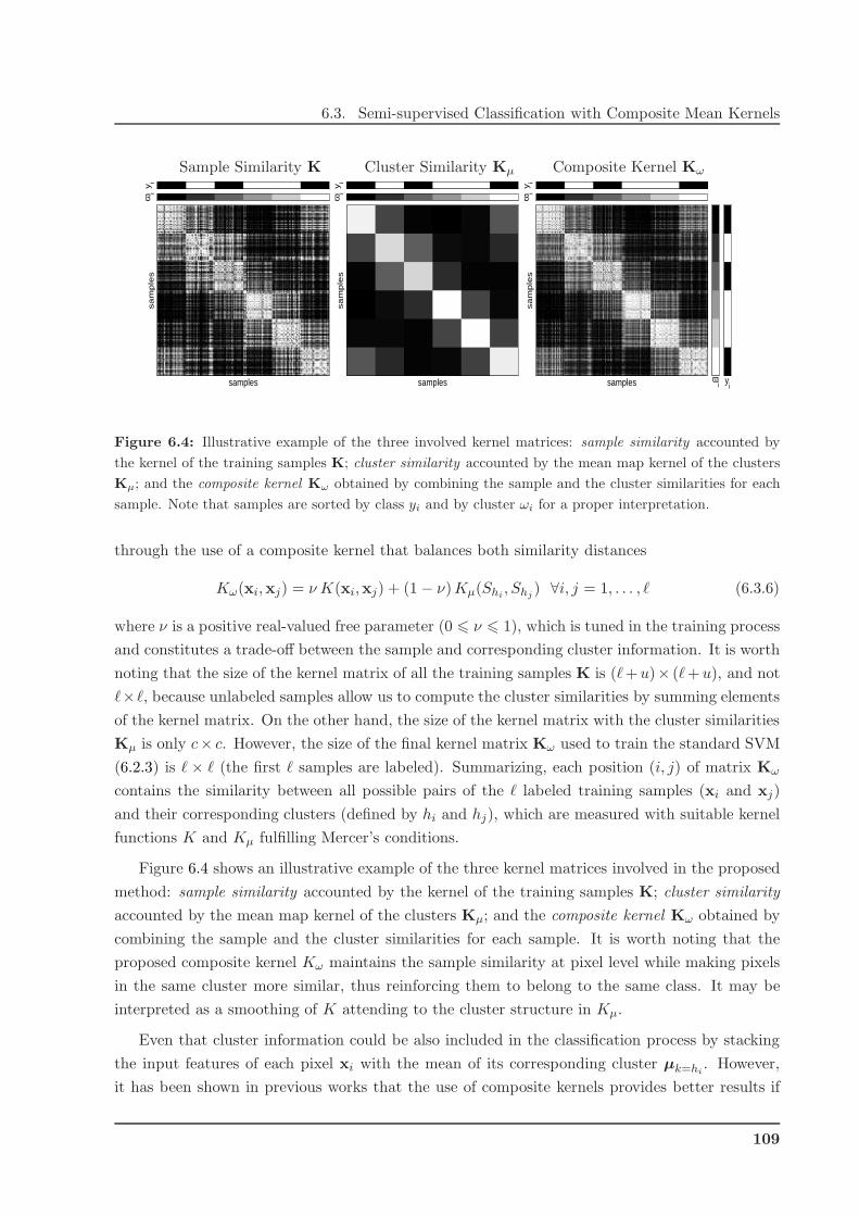
6.3. Semi-supervised Classification with Composite Mean Kernels
Sample Similarity K Cluster Similarity Kµ Composite Kernel Kω
sa
mp
les
samples ωi
ωi
yi
yi
sa
mp
les
samples ωi
ωi
yi
yi
sa
mp
les
samples ωi
ωi
yi
yi
Figure 6.4: Illustrative example of the three involved kernel matrices: sample similarity accounted by
the kernel of the training samples K; cluster similarity accounted by the mean map kernel of the clusters
Kµ; and the composite kernel Kω obtained by combining the sample and the cluster similarities for each
sample. Note that samples are sorted by class yi and by cluster ωi for a proper interpretation.
through the use of a composite kernel that balances both similarity distances
Kω(xi,xj) = ν K(xi,xj) + (1 − ν)Kµ(Shi, Shj
) ∀i, j = 1, . . . , ℓ (6.3.6)
where ν is a positive real-valued free parameter (0 6 ν 6 1), which is tuned in the training process
and constitutes a trade-off between the sample and corresponding cluster information. It is worth
noting that the size of the kernel matrix of all the training samples K is (ℓ+u)× (ℓ+u), and not
ℓ×ℓ, because unlabeled samples allow us to compute the cluster similarities by summing elements
of the kernel matrix. On the other hand, the size of the kernel matrix with the cluster similarities
Kµ is only c× c. However, the size of the final kernel matrix Kω used to train the standard SVM
(6.2.3) is ℓ× ℓ (the first ℓ samples are labeled). Summarizing, each position (i, j) of matrix Kω
contains the similarity between all possible pairs of the ℓ labeled training samples (xi and xj)
and their corresponding clusters (defined by hi and hj), which are measured with suitable kernel
functions K and Kµ fulfilling Mercer’s conditions.
Figure 6.4 shows an illustrative example of the three kernel matrices involved in the proposed
method: sample similarity accounted by the kernel of the training samples K; cluster similarity
accounted by the mean map kernel of the clusters Kµ; and the composite kernel Kω obtained by
combining the sample and the cluster similarities for each sample. It is worth noting that the
proposed composite kernel Kω maintains the sample similarity at pixel level while making pixels
in the same cluster more similar, thus reinforcing them to belong to the same class. It may be
interpreted as a smoothing of K attending to the cluster structure in Kµ.
Even that cluster information could be also included in the classification process by stacking
the input features of each pixel xi with the mean of its corresponding cluster µk=hi. However,
it has been shown in previous works that the use of composite kernels provides better results if
109

Chapter 6. Semi-supervised Cloud Classification
I1 I2 IN-1 IN
Training Images Test Image
Training Set SampleSelection
Bias
Figure 6.5: Illustrative example of the sample selection bias produced when the distributions on training
and test sets might not match, which is a common situation in remote sensing image classification if no
labeled training set is available for the test image.
different information entities are treated separately and combined in feature spaces (Mak et al.,
2004; Camps-Valls et al., 2006d, 2008a).
6.3.4 Sample Selection Bias and the Soft Mean Map
SSL methods learn from both labeled and unlabeled samples constituting the training set to
build a model that is used to classify the test set. So far we have assumed that training and test
data are independently and identically distributed (i.i.d.) from the same pdf, but in reality the
distributions on training and test sets might not match, which is known in the literature as the
sample selection bias (Heckman, 1979; Huang et al., 2007; Bickel et al., 2007) or covariate shift
(Shimodaira, 2000; Sugiyama and Muller, 2005; Sugiyama et al., 2007, 2008). Obviously, if the
training and the test data have nothing in common there is no chance to learn anything. Thus, we
assume that both follow a similar conditional distribution p(y|x) and the input distributions p(x)
differ, yet not completely (see Fig. 6.5). In remote sensing, this is a likely situation since usually
no training samples are available for the image to be classified and labeled data is extracted from
other images modeling similar problems. In these situations, not all training samples are equally
reliable. In the literature, the training samples are weighted in different ways in order to avoid
the sample selection problem: by deriving the conditional density to maximize the log-likelihood
function (Shimodaira, 2000); by changing the criterion to be maximized for learning, such as
the nonparametric kernel mean matching method presented in (Huang et al., 2007) that tries to
match the first momentum of training and test sets in the kernel space; or by modifying the model
selection criteria (importance weighted cross validation estimate of risk) to obtain unbiased results
(Sugiyama et al., 2007).
110
6.3. Semi-supervised Classification with Composite Mean Kernels
In the proposed method, the most reliable samples in terms of maximum likelihood in the
input space are used to compute a kernel function that accurately reflects the similarity between
clusters in the kernel space. Therefore, the relative reliability of training samples is trimmed by
weighting the contribution of each sample xi to the definition of the centre of mass of each cluster
in the kernel space H with the EM estimated posterior probabilities hik, that is:
φµs(Sk) =
∑
i hikφ(xi)∑
i hik, (6.3.7)
which we call the soft mean map. The corresponding kernel can be easily computed as:
KHµs
(Sk, Sl) =⟨
φµs(Sk),φµs
(Sl)⟩
=
⟨
∑
i hikφ(xi)∑
i hik,
∑
j hjlφ(xj)∑
j hjl
⟩
(6.3.8)
=
∑
i
∑
j hikhjlK(xi,xj)∑
i hik
∑
j hjl,
and now, when computing cluster similarities, all training samples contribute to all clusters but
with different relative weights with a posteriori probability sense. The main advantage of the pro-
posed method is that weights for the training samples are directly computed by taking advantage
of the full statistical information of the test data distribution without modifying the classification
problem to be solved, i.e. the same QP problem of the SVM is solved with the available standard
optimization tools. We should stress that, with this approach, the EM algorithm is applied to
the entire image in order to properly characterize the test data distribution and compute the
sample weights, but the number of unlabeled samples used to describe the clusters in the soft
mean map can be selected by the user to reduce the size of the kernel matrix and thus controlling
the computational effort.
Note that the mean map kernel in (6.3.3) is a particular case of the proposed soft mean map
kernel in (6.3.8) when the training samples are associated only with one cluster (crisp association),
i.e. when hik = 1 if xi belongs to cluster ωk and hik = 0 otherwise. In addition, the expression of
the soft mean map kernel in (6.3.8) can be rewritten in matrix notation as follows:
KHµ = DH⊤KHD (6.3.9)
where K is the (ℓ + u) × (ℓ + u) kernel matrix of both labeled and unlabeled training samples;
H is a (ℓ + u) × c matrix containing the membership value hik of each training sample to each
cluster of the analyzed image; and D is a c×c diagonal matrix with normalization factors for each
cluster Dkk =∑
i hik. Note that the computational effort is directly controlled by the number of
unlabeled samples u included in K to describe the clusters.
The size of the matrix containing the similarity between clusters Kµ is c× c. Thus, it has to
be expanded to match the number of labeled samples, in order to obtain the final ℓ × ℓ kernel
matrix Kω in (6.3.6) used to train the classifier:
Kω = ν JKJ⊤ + (1 − ν)WKµW⊤ (6.3.10)
111
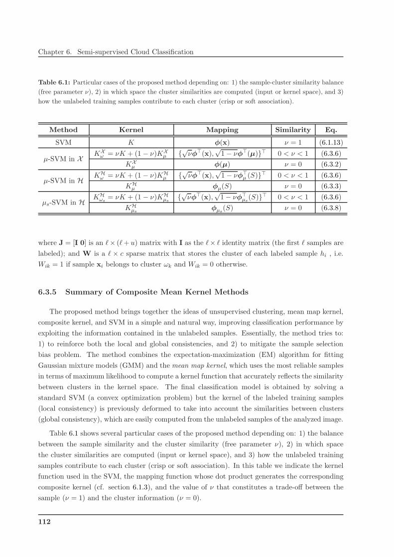
Chapter 6. Semi-supervised Cloud Classification
Table 6.1: Particular cases of the proposed method depending on: 1) the sample-cluster similarity balance
(free parameter ν), 2) in which space the cluster similarities are computed (input or kernel space), and 3)
how the unlabeled training samples contribute to each cluster (crisp or soft association).
Method Kernel Mapping Similarity Eq.
SVM K φ(x) ν = 1 (6.1.13)
µ-SVM in X KXω = νK + (1 − ν)KX
µ {√νφ⊤(x),√
1 − νφ⊤(µ)}⊤ 0 < ν < 1 (6.3.6)
KXµ φ(µ) ν = 0 (6.3.2)
µ-SVM in H KHω = νK + (1 − ν)KH
µ {√νφ⊤(x),√
1 − νφ⊤µ (S)}⊤ 0 < ν < 1 (6.3.6)
KHµ φµ(S) ν = 0 (6.3.3)
µs-SVM in H KHωs
= νK + (1 − ν)KHµs
{√νφ⊤(x),√
1 − νφ⊤µs
(S)}⊤ 0 < ν < 1 (6.3.6)
KHµs
φµs(S) ν = 0 (6.3.8)
where J = [I 0] is an ℓ× (ℓ+ u) matrix with I as the ℓ× ℓ identity matrix (the first ℓ samples are
labeled); and W is a ℓ × c sparse matrix that stores the cluster of each labeled sample hi , i.e.
Wik = 1 if sample xi belongs to cluster ωk and Wik = 0 otherwise.
6.3.5 Summary of Composite Mean Kernel Methods
The proposed method brings together the ideas of unsupervised clustering, mean map kernel,
composite kernel, and SVM in a simple and natural way, improving classification performance by
exploiting the information contained in the unlabeled samples. Essentially, the method tries to:
1) to reinforce both the local and global consistencies, and 2) to mitigate the sample selection
bias problem. The method combines the expectation-maximization (EM) algorithm for fitting
Gaussian mixture models (GMM) and the mean map kernel, which uses the most reliable samples
in terms of maximum likelihood to compute a kernel function that accurately reflects the similarity
between clusters in the kernel space. The final classification model is obtained by solving a
standard SVM (a convex optimization problem) but the kernel of the labeled training samples
(local consistency) is previously deformed to take into account the similarities between clusters
(global consistency), which are easily computed from the unlabeled samples of the analyzed image.
Table 6.1 shows several particular cases of the proposed method depending on: 1) the balance
between the sample similarity and the cluster similarity (free parameter ν), 2) in which space
the cluster similarities are computed (input or kernel space), and 3) how the unlabeled training
samples contribute to each cluster (crisp or soft association). In this table we indicate the kernel
function used in the SVM, the mapping function whose dot product generates the corresponding
composite kernel (cf. section 6.1.3), and the value of ν that constitutes a trade-off between the
sample (ν = 1) and the cluster information (ν = 0).
112
6.3. Semi-supervised Classification with Composite Mean Kernels
6.3.6 Performance on Synthetic Data
Figure 6.6 shows an illustrative example of how the proposed method efficiently exploits the
information contained in the available unlabeled samples to characterize the marginal distribution
of data by means of the cluster structure. In order to demonstrate the robustness of the method
in the sample selection bias problem, we used a two-dimenssional non-linear classification problem
where training and test data are generated by two slightly different mixture models composed of
six Gaussian components (Fig. 6.6[top]). Three different models are obtained in order to illustrate
the trade-off between the sample (ν = 1) and the cluster information (ν = 0) provided by the
proposed method (Fig. 6.6[bottom]). In particular, we have depicted results of the pixel-based
approach (ν = 1) equivalent to a standard SVM trained with K (left); the cluster-based approach
(ν = 0) of the µs-SVM trained with KHµs
(center); and the composite pixel-cluster approach
(0 < ν < 1) of the µs-SVM trained with KHωs
(right).
Selected models are compared with the classification boundary of the maximum likelihood
classifier (MLC) built with the true mixture models (upper-bound of the classification perfor-
mance) of both the training distribution and the test distribution, respectively. In the three plots
at the bottom part of the figure, we can observe from the sample-similarity based approach to
the cluster-similarity based approach, how the classification boundary changes. On the one hand,
Fig. 6.6(d) corresponds to the standard SVM looking for a maximum margin classifier of the
training samples. In this case, the classification boundary matches the MLC boundary of the
training set (gold line). On the other hand, Fig. 6.6(e) corresponds to the cluster-based approach
that trains a SVM using as kernel matrix the cluster similarity KHµs
of the associated clusters.
In this case, classification boundary is dominated by the cluster distribution of the unlabeled
samples form the test set, and thus it matches the MLC boundary of the test set (blue line). It is
worth noting that in the case where both sample and cluster similarities are combined (Fig. 6.6(f))
we obtain an intermediate solution, that is: 1) in regions densely populated by labeled training
samples, the µs-SVM follows the optimal MLC boundary of the training data (middle-left part
of the plot); and 2) in regions without labeled training samples forcing the output class, µs-SVM
follows the optimal MLC boundary of the test data (bottom-right corner of the plot). The value
of ν can be tuned by the user in the training process or selected through cross-validation in the
training set, as is commonly done with the other free parameters of SVMs, such as C and σ. We
should note, however, that the model selection in semi-supervised methods applied to problems
affected by sample selection bias is not well-solved since, if the training and test distributions are
significantly different, selected model will be biased towards the training samples when performing
cross-validation in the training set.
To provide an exhaustive analysis of the proposed method’s performance, the experiment
described in Fig. 6.6 was repeated for a series of realizations varying the following parameters:
• Data Generation: the width σ of the Gaussian components used in the mixture model to
generate the training and test data. Different σ correspond to different levels of data overlap
113

Chapter 6. Semi-supervised Cloud Classification
(a) Training Data (b) Test Data (c) Cluster Distribution
(d) SVM (K)
(e) µs-SVM (KHµs
)
(f) µs-SVM (KHωs
)
Figure 6.6: Illustrative example of the use of composite mean kernel in a two-dimensional two-classes
problem where training and test data are generated by two slightly different mixture models composed
of six Gaussian components. Upper part of the figure (left and center) shows the samples (circles) and
the distribution (colored areas) of each Gaussian component of the the training (6 × 25 samples) ant test
(6 × 1000 samples) sets, respectively. Upper-right plot shows test samples with the true class labels (red
and black points) and the distribution (shaded areas) of the found clusters by the EM algorithm. Bottom
part of the figure shows the classification results of the proposed composite kernel using the soft mean
map for three different situations: pixel-based approach (ν = 1) equivalent to a standard SVM trained
with K (left); cluster-based approach (ν = 0) of the µs-SVM trained with KHµs
(center); and composite
pixel-cluster approach (0 < ν < 1) of the µs-SVM trained with KHωs
(right). In these plots, red and
black points represent the training samples; blue circles indicate the samples used as support vectors in
each model; golden line and shaded areas indicate the classification boundary of the maximum likelihood
classifier (MLC) built with the true mixture model of the training data (upper-bound of the classification
performance); blue line indicates the classification boundary of the MLC built with the true mixture model
of the test data; and black line shows the classification boundary of the trained models.
114
6.3. Semi-supervised Classification with Composite Mean Kernels
that determine the clasification complexity. In particular, using the true pdf that generated
the test data with σ = {0.2, 0.275, 0.35, 0.425, 0.5}, the maximum likelihood classifier results
in a kappa statistic κ = {0.97, 0.90, 0.81, 0.71, 0.63}, respectively. Fig. 6.7(a) shows the κ
obtained when classifying test data with the MLC using the true pdf of the test data (dashed
line), which provides an upper-bound of the classification performance, and using the true
pdf of the training data (dotted line), which informs us about the difference between the
mixture models used to generate training and test data (sample selection bias problem).
• Supervised Information: the number of labeled samples ℓ used to train the models. By
decreasing the number of labeled training samples ℓ, one can analyze how the SSL method
efficiently exploits the information contained in the available unlabeled samples. In the
experiments, the number of unlabeled samples is fixed to u = 300 and we explore from
ill-posed situations with only 3 labeled samples per class (ℓ = 6) up to almost supervised
cases with 300 labeled samples per class (ℓ = 600).
• Unsupervised Clustering: the number of clusters c, i.e. the number of Gaussian components
fixed in the EM algorithm. The proposed method requires as input the clusters presents
in the test data, which are obtained from the unlabeled data using the EM algorithm.
Therefore, the proposed method relies on the clustering performance and assumes that
clusters present in the test data are correctly identified. In order to analyze the robustness
of the method to inaccurate clustering results, the number of Gaussian components in the
EM algorithm is set to c = {2, 4, 6, 8, 10} instead of the actual six components of the mixture
model that generated the data.
As mentioned above, for the experiments, we generated training sets consisting of ℓ = 600 labeled
samples (300 samples per class), and added u = 300 unlabeled (randomly selected) samples from
the analyzed test data to the training set for the SSL methods. We focus on the ill-posed scenario
and vary the rate of labeled samples, i.e. {1, 2, 4, 8, 14, 27, 52, 100}% of the labeled samples of the
training set were used to train the models in each experiment. In order to avoid skewed conclu-
sions, for each combination of parameters σ, ℓ, and c, the experiments were run for ten realizations
where the used training samples were randomly selected. All classifiers are compared using the
estimated kappa statistic κ as a measure of robustness in the classification of 6000 independent
validation samples. Free parameter ν was varied in steps of 0.1 in the range [0.01, 0.99], and the
Gaussian width for the RBF kernel was tuned in the range σRBF = {10−3, . . . , 10}. The selection
of the best subset of free parameters was done by cross-validation.
Fig. 6.7 shows the validation results for the analyzed SVM-based classifiers when the number
of clusters in the EM is fixed to the c = 6 actual clusters and only class overlap σ and labeled
training samples ℓ are varied. Fig. 6.7(b) and 6.7(c) show the κ surface as a function of σ and ℓ for
the proposed µs-SVM method when using as kernel KHµs
(ν = 0) andKHωs
(0 < ν < 1), respectively.
These plots illustrate how the most separated are the classes (low σ) and supervised information
is available (high ℓ), the most accurate is the classification for all methods. Fig. 6.7[bottom] shows
115

Chapter 6. Semi-supervised Cloud Classification
0.2 0.25 0.3 0.35 0.4 0.45 0.50.5
0.6
0.7
0.8
0.9
1
σ
Kap
pa s
tatis
tic,κ
MLC on test set (upper−bound)
Test set pdfTraining set pdf
(a)
6 12 24 48 84 162312600
0.20.275
0.350.425
0.5
0.2
0.4
0.6
0.8
1
labeled samples
µs−SVM (Kµ
H)
σK
appa
sta
tistic
, κ
(b)
6 12 24 48 84 162312600
0.20.275
0.350.425
0.5
0.2
0.4
0.6
0.8
1
labeled samples
µs−SVM (Kω
H)
σ
Kap
pa s
tatis
tic, κ
(c)
6 12 24 48 84 162 312 6000.5
0.55
0.6
0.65
0.7
0.75
labeled samples
Kap
pa s
tatis
tic,
avg(
κ)
SVM on µk (K)
SVM on xi (K)
µ−SVM (KµX)
µ−SVM (KωX)
µs−SVM (K
µH)
µs−SVM (K
ωH)
(d)
6 12 24 48 84 162 312 6000.05
0.1
0.15
0.2
0.25
labeled samples
Kap
pa s
tatis
tic,
std(
κ)
(e)
6 12 24 48 84 162 312 60020
30
40
50
60
70
80
90
100
labeled samples
% o
f SV
s
(f)
Figure 6.7: Validation results for the analyzed SVM-based classifiers when the number of clusters in the
EM is fixed to the actual clusters (c = 6) and only class overlap σ and labeled training samples ℓ are
varied. Top, from left to right : MLC kappa statistic (κ) for different levels of data overlap σ using the test
and the training pdfs, and κ surface as a function of σ and number of labeled samples ℓ for the proposed
µs-SVM method when using as kernel KHµs
(ν = 0) and KHωs
(0 < ν < 1). Bottom, from left to right : results
averaged over σ for all the analyzed methods: avg(κ), std(κ), and the percentage of training samples used
as support vectors SVs[%].
the results for all the analyzed methods averaged over σ: avg(κ), std(κ), and the percentage of
training samples used as support vectors (SVs) in the selected models. Note that, in addition
to the standard SVM and the variations of the proposed method, we have include classification
results obtained when using the trained standard SVM (K) to classify the centers of the clusters
(µk) and then assigning the same class label to all the samples belonging to the same cluster ωk.
Several conclusions can be obtained from these plots. First (Fig. 6.7(d)), composite mean kernels
classifiers (black ‘+’ lines), which combine both sample and cluster similarities, produce better
classification results than SVM (red dotted line) in all cases for both the KXω and KH
ωskernels
(note that SVM is a particular case of the µ-SVM for ν = 1). The cluster-based approaches KXµ
and KHµs
(blue ‘◦’ lines) provide accurate classifications when there are enough labeled samples
to describe the class conditional distribution of the clusters (otherwise a whole cluster can be
misclassified). In addition, cluster-based approaches are not equivalent to a simple classification
of the centers of the clusters (red dash-doted line). Regarding the standard deviation of kappa
std(κ) (Fig. 6.7(e)), the SVM provide the most stable results, but composite mean kernels provide
116
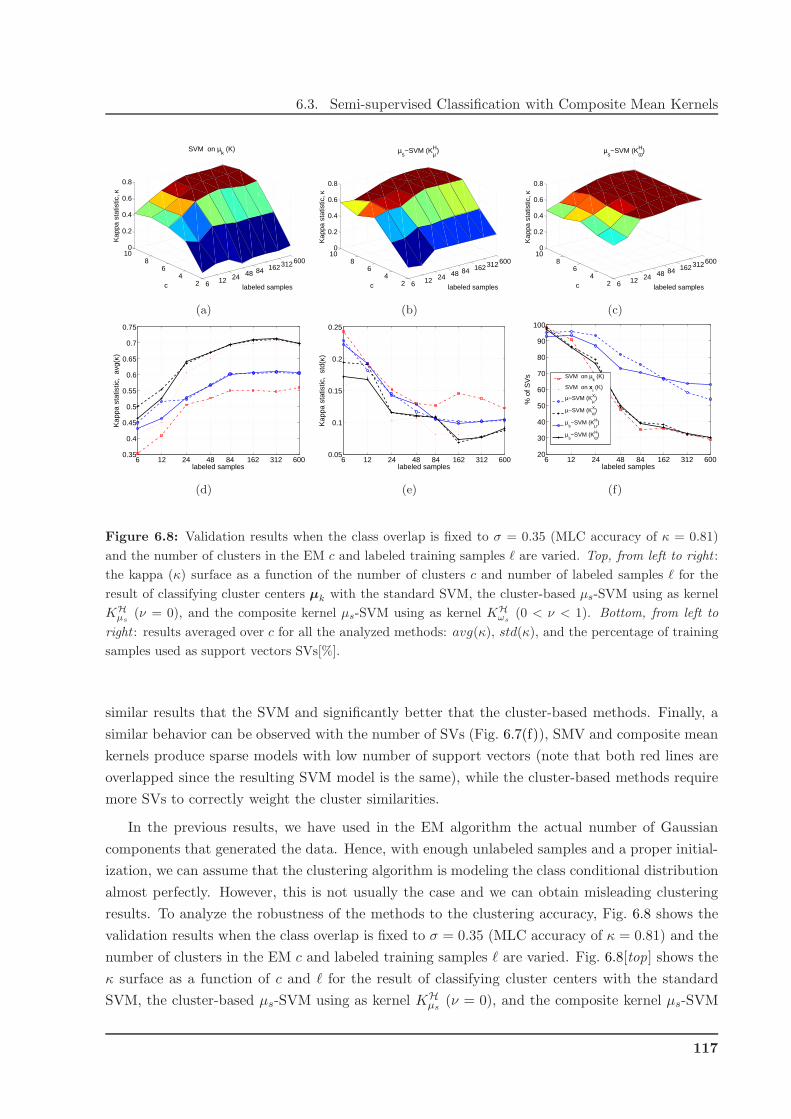
6.3. Semi-supervised Classification with Composite Mean Kernels
6 12 24 48 84 162312600
24
68
100
0.2
0.4
0.6
0.8
labeled samples
SVM on µk (K)
c
Kap
pa s
tatis
tic, κ
(a)
6 12 24 48 84 162312600
24
68
100
0.2
0.4
0.6
0.8
labeled samples
µs−SVM (Kµ
H)
c
Kap
pa s
tatis
tic, κ
(b)
6 12 24 48 84 162312600
24
68
100
0.2
0.4
0.6
0.8
labeled samples
µs−SVM (Kω
H)
c
Kap
pa s
tatis
tic, κ
(c)
6 12 24 48 84 162 312 6000.35
0.4
0.45
0.5
0.55
0.6
0.65
0.7
0.75
labeled samples
Kap
pa s
tatis
tic,
avg(
κ)
(d)
6 12 24 48 84 162 312 6000.05
0.1
0.15
0.2
0.25
labeled samples
Kap
pa s
tatis
tic,
std(
κ)
(e)
6 12 24 48 84 162 312 60020
30
40
50
60
70
80
90
100
labeled samples
% o
f SV
s
SVM on µk (K)
SVM on xi (K)
µ−SVM (KµX)
µ−SVM (KωX)
µs−SVM (K
µH)
µs−SVM (K
ωH)
(f)
Figure 6.8: Validation results when the class overlap is fixed to σ = 0.35 (MLC accuracy of κ = 0.81)
and the number of clusters in the EM c and labeled training samples ℓ are varied. Top, from left to right :
the kappa (κ) surface as a function of the number of clusters c and number of labeled samples ℓ for the
result of classifying cluster centers µk with the standard SVM, the cluster-based µs-SVM using as kernel
KHµs
(ν = 0), and the composite kernel µs-SVM using as kernel KHωs
(0 < ν < 1). Bottom, from left to
right : results averaged over c for all the analyzed methods: avg(κ), std(κ), and the percentage of training
samples used as support vectors SVs[%].
similar results that the SVM and significantly better that the cluster-based methods. Finally, a
similar behavior can be observed with the number of SVs (Fig. 6.7(f)), SMV and composite mean
kernels produce sparse models with low number of support vectors (note that both red lines are
overlapped since the resulting SVM model is the same), while the cluster-based methods require
more SVs to correctly weight the cluster similarities.
In the previous results, we have used in the EM algorithm the actual number of Gaussian
components that generated the data. Hence, with enough unlabeled samples and a proper initial-
ization, we can assume that the clustering algorithm is modeling the class conditional distribution
almost perfectly. However, this is not usually the case and we can obtain misleading clustering
results. To analyze the robustness of the methods to the clustering accuracy, Fig. 6.8 shows the
validation results when the class overlap is fixed to σ = 0.35 (MLC accuracy of κ = 0.81) and the
number of clusters in the EM c and labeled training samples ℓ are varied. Fig. 6.8[top] shows the
κ surface as a function of c and ℓ for the result of classifying cluster centers with the standard
SVM, the cluster-based µs-SVM using as kernel KHµs
(ν = 0), and the composite kernel µs-SVM
117
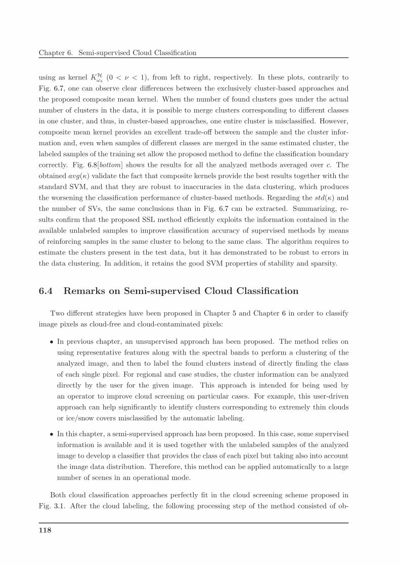
Chapter 6. Semi-supervised Cloud Classification
using as kernel KHωs
(0 < ν < 1), from left to right, respectively. In these plots, contrarily to
Fig. 6.7, one can observe clear differences between the exclusively cluster-based approaches and
the proposed composite mean kernel. When the number of found clusters goes under the actual
number of clusters in the data, it is possible to merge clusters corresponding to different classes
in one cluster, and thus, in cluster-based approaches, one entire cluster is misclassified. However,
composite mean kernel provides an excellent trade-off between the sample and the cluster infor-
mation and, even when samples of different classes are merged in the same estimated cluster, the
labeled samples of the training set allow the proposed method to define the classification boundary
correctly. Fig. 6.8[bottom] shows the results for all the analyzed methods averaged over c. The
obtained avg(κ) validate the fact that composite kernels provide the best results together with the
standard SVM, and that they are robust to inaccuracies in the data clustering, which produces
the worsening the classification performance of cluster-based methods. Regarding the std(κ) and
the number of SVs, the same conclusions than in Fig. 6.7 can be extracted. Summarizing, re-
sults confirm that the proposed SSL method efficiently exploits the information contained in the
available unlabeled samples to improve classification accuracy of supervised methods by means
of reinforcing samples in the same cluster to belong to the same class. The algorithm requires to
estimate the clusters present in the test data, but it has demonstrated to be robust to errors in
the data clustering. In addition, it retains the good SVM properties of stability and sparsity.
6.4 Remarks on Semi-supervised Cloud Classification
Two different strategies have been proposed in Chapter 5 and Chapter 6 in order to classify
image pixels as cloud-free and cloud-contaminated pixels:
• In previous chapter, an unsupervised approach has been proposed. The method relies on
using representative features along with the spectral bands to perform a clustering of the
analyzed image, and then to label the found clusters instead of directly finding the class
of each single pixel. For regional and case studies, the cluster information can be analyzed
directly by the user for the given image. This approach is intended for being used by
an operator to improve cloud screening on particular cases. For example, this user-driven
approach can help significantly to identify clusters corresponding to extremely thin clouds
or ice/snow covers misclassified by the automatic labeling.
• In this chapter, a semi-supervised approach has been proposed. In this case, some supervised
information is available and it is used together with the unlabeled samples of the analyzed
image to develop a classifier that provides the class of each pixel but taking also into account
the image data distribution. Therefore, this method can be applied automatically to a large
number of scenes in an operational mode.
Both cloud classification approaches perfectly fit in the cloud screening scheme proposed in
Fig. 3.1. After the cloud labeling, the following processing step of the method consisted of ob-
118
6.4. Remarks on Semi-supervised Cloud Classification
taining the final abundance fraction of clouds for all image pixels. In the unsupervised approach,
the improved cloud product map was obtained combining the Cloud Abundance, aiC , and the
Cloud Probability, hiC , by means of a pixel-by-pixel multiplication, ϑi = aiChiC . The procedure
followed in section 5.3 to obtain the cloud final product is still valid for the semi-supervised ap-
proach. The main difference now is that, instead of obtaining hiC from the posterior probabilities
of the cloud-clusters for each sample provided by the EM algorithm, we define hiC as the hard
classification label yi provided for each sample by the semi-supervised cloud classifier. That is,
hiC = 1 if the sample xi is classified as cloud-contaminated (C) and hiC = 0 if is cloud-free.
It is worth noting that now hiC is a binary label instead of a continuous probability value, but
it indicates more accurately the presence of cloud. In addition, the posterior probabilities also
decreased drastically from one to zero in the boundaries between clusters. Therefore, both the
cloud probability and the cloud classification label indicate if one pixel is cloudy, C, or cloud-free,
C, but none of them give information about the cloud content at subpixel level. In the cloud final
product, ϑi = aiChiC , hiC indicates the cloudy pixels and aiC indicates their cloud abundance.
119

Chapter 6. Semi-supervised Cloud Classification
120

Part III
Experimental Results


Chapter 7
Unsupervised Cloud Screening
Validation
The third part of the work deals with the validation of the proposed methodology and cloud
products. A wide database of images has been included in the study in order to take into account
the different peculiarities of the problem: geographic location, date and season, type of cloud, and
type of surface. The selected images allow us to validate method’s performance since they include
different landscapes, vegetation, bare soils, and two critical cases given the especial characteristics
of the induced problems: ice and snow covers.
The validation of cloud screening algorithms is not an easy task because, in the unsupervised
case (i.e. with no labeled data), there are no simultaneous independent measurements with
the same spatial resolution. In most cases, the performance of cloud detection algorithms has
been evaluated against visual analysis of the original satellite images. The human eye is able
to recognize cloud structures in a satellite image much better than any automatic algorithm
does, which justifies this validation approach. However, human cloud recognition may miss the
difficult cases (thin clouds, broken cloudiness) and is far from being operational. In addition,
visual comparison requires a large amount of tedious work, which is unsuited for a quantitative
validation on a large dataset. For these reasons, a significant effort has been done in order to
validate results by using different techniques:
• The simplest approach consists in comparing the final cloud mask and abundance with
a false color composite of the images. Therefore, the resulting products are validated by
visual inspection on CHRIS and MERIS data in section 7.1 and section 7.2, respectively.
Following this validation approach, we are simultaneously testing the generalization abil-
ity of the proposed cloud screening algorithm, because a general methodology for cloud
detection should be valid for different sensors working in the VNIR range. In particular,
in Gomez-Chova et al. (2005b,a), performance of the proposed approach is tested on im-
ages from the CHRIS instrument, which presents completely different characteristics than
Chapter 7. Unsupervised Cloud Screening Validation
MERIS, tested in Gomez-Chova et al. (2005c, 2006d, 2007a).
• In the case of MERIS, we can also compare results with the official MERIS Level 2 Cloud
Flag. In section 7.3, a representative set of MERIS images is processed and compared to
the Level 2 products (used for validation purposes only) by comparing its cloud flag product
to the cloud mask produced by the presented method. Preliminary test of this approach
were carried out in previous works (Gomez-Chova et al., 2005c, 2006d, 2007a) by testing
critical situations in cloud detection (e.g. ice/snow covers). Results were encouraging since
the proposed algorithm classifies difficult cloud pixels more accurately; especially thin cirrus
clouds and clouds over ice/snow.
• The lack of a real ground truth, and the low accuracy shown by the official MERIS Level
2 Cloud Flag in some situations prevent the validation of the cloud screening in fair condi-
tions. Therefore, new validation approaches are required in order to test the proposed cloud
screening algorithm. In section 7.4, the performance of the cloud screening is tested with a
multitemporal validation approach proposed in Gomez-Chova et al. (2006f). In particular,
pairs of cloud-free and cloud-covered images over the same area are used to detect cloud-
pixels by identifying pixels with spectral changes between both dates. The spectral change
is detected by using the spectral angle distance (SAD) as it is invariant to multiplicative
scaling (being less affected by atmospheric and illumination changes). Image pairs are se-
lected to be close in time, so spectral changes due to temporal evolution of the surface are
avoided. However, images taken from orbits within three or six days present a significant
variation in the viewing geometry. Therefore, pixels with significant changes in composition
(> 10%) due to the different observation angle are not considered in the multi-temporal
cloud screening validation.
In the following sections, we present results of the unsupervised cloud screening scheme pro-
posed in Chapter 5. The results were obtained for all images and scenarios as follows. The
number of clusters found by the EM clustering was automatically determined as the maximum
of suggested numbers by the DB and MDL indices (cf. section 5.2.1). However, we did not
observe a critical dependence of the results on the number of clusters; note that even if a low
number of clusters is selected, some of them should correspond to different cloud types, since the
(overgrown) ROI is typically well-identified. Clusters were labeled into geo-physical classes by an
operator considering the extracted features (cf. section 5.2.2). The number of endmembers was
equal to the number of cloud-free clusters (cf. section 5.3.1). Finally, cloud screening results are
presented in terms of the cloud probability hiC in (5.2.8), the cloud abundance aiC in (5.3.4), and
the hard classification between clouds and ground was obtained applying a threshold of 0.05 to
the cloud final product ϑ in (5.3.5) (cf. section 5.3.3).
124
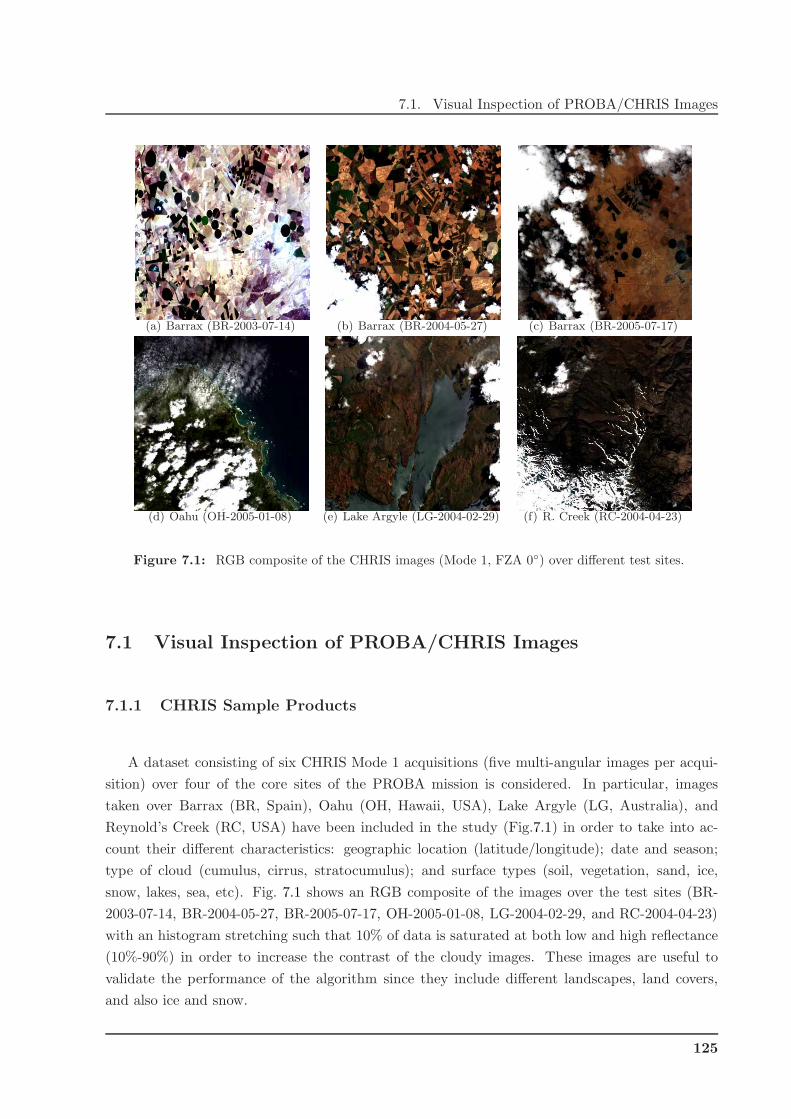
7.1. Visual Inspection of PROBA/CHRIS Images
(a) Barrax (BR-2003-07-14) (b) Barrax (BR-2004-05-27) (c) Barrax (BR-2005-07-17)
(d) Oahu (OH-2005-01-08) (e) Lake Argyle (LG-2004-02-29) (f) R. Creek (RC-2004-04-23)
Figure 7.1: RGB composite of the CHRIS images (Mode 1, FZA 0◦) over different test sites.
7.1 Visual Inspection of PROBA/CHRIS Images
7.1.1 CHRIS Sample Products
A dataset consisting of six CHRIS Mode 1 acquisitions (five multi-angular images per acqui-
sition) over four of the core sites of the PROBA mission is considered. In particular, images
taken over Barrax (BR, Spain), Oahu (OH, Hawaii, USA), Lake Argyle (LG, Australia), and
Reynold’s Creek (RC, USA) have been included in the study (Fig.7.1) in order to take into ac-
count their different characteristics: geographic location (latitude/longitude); date and season;
type of cloud (cumulus, cirrus, stratocumulus); and surface types (soil, vegetation, sand, ice,
snow, lakes, sea, etc). Fig. 7.1 shows an RGB composite of the images over the test sites (BR-
2003-07-14, BR-2004-05-27, BR-2005-07-17, OH-2005-01-08, LG-2004-02-29, and RC-2004-04-23)
with an histogram stretching such that 10% of data is saturated at both low and high reflectance
(10%-90%) in order to increase the contrast of the cloudy images. These images are useful to
validate the performance of the algorithm since they include different landscapes, land covers,
and also ice and snow.
125

Chapter 7. Unsupervised Cloud Screening Validation
7.1.2 CHRIS Cloud Screening Results
We have tested the proposed scheme for the aforementioned images. All the method has been
implemented in Matlab programming language and it is capable to handle directly the CHRIS
HDF original files and process them automatically producing the results in an ENVI standard
format. Intermediate images of the method have been shown in Chapter 5. This section analyzes
the performance of the method on the six images by means of the thematic map of the clusters
and the cloud abundance product (Fig.7.2).
The following conclusions about the method results are depicted in Fig.7.2. The three images
over the Barrax (BR, Spain) site are a good example of an easy cloud detection problem, when
clearly defined clouds are well contrasted with soil and vegetation. The ROI selection can be
easily appreciated in the classified images, being more important in the BR-2003-07-14 image
where small clouds could be mixed in a cluster with other classes if the whole image is considered.
At the OH-2005-01-08 image (Oahu, Hawaii), waves and beach sand pixels belong to a cluster
labeled as cloud due to their high reflectance and whiteness, but they present low probabilities
and abundances. In addition, this image presents cirrus clouds over land and over sea that are well
detected since specific clusters describe them and have been correctly classified. One of the weak
points of the algorithm is the use of thresholds to select the ROI, because some thin or small clouds
can be excluded from the ROI. A solution is to relax thresholds at the risk of considering as ROI
the whole image like in the image of LG-2004-02-29 (Lake Argyle, Australia). But, even in this
case, results are good if clouds cover a sufficient percentage of the image or the number of clusters
is high enough. The image of RC-2004-04-23 (Reynold’s Creek, United States) is an example of
one of the critical issues in cloud detection, the presence of ice/snow in the surface. These covers
and clouds have a similar reflectance behavior. However, the atmospheric absorption suffered by
cloud pixels is lower than for the case of surface pixels due to their height, thus different clusters
are found for these two classes in the image. Thanks to the extracted atmospheric features,
ice/snow pixels present low cloud probability values although the cloud abundance provided by
the spectral unmixing could be relatively high due to the spectral similarities. In consequence,
both information types are combined improving the final classification accuracy.
The use of CHRIS data allows us to assess algorithm performance in favorable spatial reso-
lution (34 m) and number of bands (62 channels). The extrapolation to the ENVISAT MERIS
sensor will be very valuable in order to simulate the subpixel effects due to the MERIS coarse
spatial resolution (300m at Full Resolution). In addition, MERIS allows an accurate oxygen ab-
sorption estimation (11th/10th band ratio) and presents narrower bands to enhance detection
and knowledge discovery.
126

7.1. Visual Inspection of PROBA/CHRIS Images
Figure 7.2: Cloud screening results on CHRIS images: BR-2003-07-14, BR-2004-05-27, BR-2005-07-17,
OH-2005-01-08, LG-2004-02-29, and RC-2004-04-23 (from left to right). First and third rows: Thematic
maps obtained after the cluster labeling (colors have been manually assigned to match land cover colors:
clouds in grey, ground in brown, ice/snow in yellow, and background in blue). Second and fourth rows :
Cloud abundance product.
127

Chapter 7. Unsupervised Cloud Screening Validation
(a) Barrax (BR-2003-07-14) (b) Barrax (BR-2004-07-14) (c) Finland (FI-2005-02-26) (d) France (FR-2005-03-19)
Figure 7.3: RGB composite of the MERIS images over the test sites of Barrax, Finland, and France.
7.2 Visual Inspection of ENVISAT/MERIS Images
7.2.1 MERIS Sample Products
A dataset consisting of four acquisitions over three sites has been selected to perform the
visual validation on MERIS data. Both Level 1b (L1b) and Level 2 (L2) products were avail-
able for all MERIS Full Resolution (FR) images (300 m). In particular, the site of Barrax (BR,
Spain) was selected as the main test site since it has been the core site of previous Earth ob-
servation campaigns and the analyzed cloudy images are part of the data acquired in the frame-
work of the SPARC 2003 and 2004 ESA campaigns (ESA-SPARC Project, contract ESTEC-
18307/04/NL/FF) (Moreno et al., 2005). These two images were acquired on July 14th of two
consecutive years (BR-2003-07-14 and BR-2004-07-14). Additionally, MERIS acquisitions over
France (FR-2005-03-19) and Finland (FI-2005-02-26) have been included in the study in order
to take into account their different characteristics: geographic location, date and season, type
of cloud, and type of surface. Again, the selected images represent different scenarios extremely
useful to validate the performance of the method, including different landscapes; soils covered by
vegetation or bare; and two critical cases given the special characteristics of the induced problems:
ice and snow. Fig. 7.3 shows an RGB composite of the images over the test sites (BR-2003-07-14,
BR-2004-07-14, FI-2005-02-26, and FR-2005-03-19) with an histogram stretching such that 10%
of data is saturated at both low and high reflectance (10%-90%) in order to increase the contrast
of the cloudy images.
The proposed method is only applied to the MERIS L1b products (TOA radiance) because
the top of aerosols reflectance provided on MERIS L2 products does not include information
at the oxygen and water vapor absorptions (MERIS channels 11 and 15 are not corrected from
atmosphere due to the strong gaseous absorptions). Besides, L2 products are processed from L1b
using a cloud pixel classification that could be inaccurate. Therefore, L2 products are only used
for validation purposes by comparing the official L2 cloud flag with the cloud mask produced by
our method.
128

7.2. Visual Inspection of ENVISAT/MERIS Images
7.2.2 MERIS Cloud Screening Results
Easy cloud screening situations
The two images over Barrax (Spain) are a good example of an easy cloud detection problem,
where opaque clouds are well contrasted with bare soil and vegetation (Fig. 7.4[first and second
columns]). At the BR-2003-07-14 image, dry soil pixels belong to a cluster labeled as cloud due to
their high reflectance and whiteness, but they present low probabilities and abundances. The BR-
2004-07-14 image presents thin and small clouds over land and over sea, which are well detected
since a specific cluster describes them. The ROI selection can be easily seen in the classification
images (Fig. 7.4[second row ]), being more significant in the BR-2004-07-14 image where small
clouds could be mixed in a cluster with other ground covers if the whole image is considered.
The use of thresholds to select the ROI could be interpreted as one of the weak points of the
algorithm, since some thin or small clouds could be potentially excluded from the ROI. However,
the ROI selection can be seen as an eventual improvement. The obvious solution is to relax the
thresholds or even consider the whole image. In this case, results are accurate if clouds cover a
sufficient percentage of the image or the found number of clusters is high enough (as in the image
over Finland, FI-2005-02-26).
Challenging cloud screening situations
The images over Finland and France have been included in the study to test one of the critical
issues in cloud screening for which the proposed algorithm was intended for. In particular, the
presented approach is designed to overcome the presence of bright pixels, such as ice and snow
in the surface. Bright land covers and clouds have a similar reflectance behavior, thus thresholds
on reflectance values or unmixed fractions do not solve the problem. However, the atmospheric
absorption suffered by cloud pixels is lower than for the surface pixels due to their height. For
this reason, when using together all the features in the clustering algorithm, different clusters are
found for these two classes in the image. Thanks to the extracted atmospheric features, ice/snow
pixels present low cloud probability values although the cloud abundance provided by the spectral
unmixing could be relatively high due to the spectral similarities.
Consequently, both information types are combined improving the final cloud abundance prod-
uct provided to the users (Fig. 7.4[third row ]). Figure 7.4[fourth column] shows a case example
result for an image over France (FR-2005-03-19) that presents opaque clouds at south and north
France, and snowy mountains at various altitudes (Pyrenees, Massif Central, and the Alps),
which are well-distinguished from clouds. The cloud product for these regions presents low values
because the low cloud probability, hiC ∼ 0, obtained for these pixels.
In the case of Finland (FI-2005-02-26, Fig. 7.4[third column]), we have a different scenario
where a cirrus cloud, often found in advance of a warm front, is moving from sea to the icy coast
of Finland. In this image, we have a difficult cloud identification problem, even for an expert
129
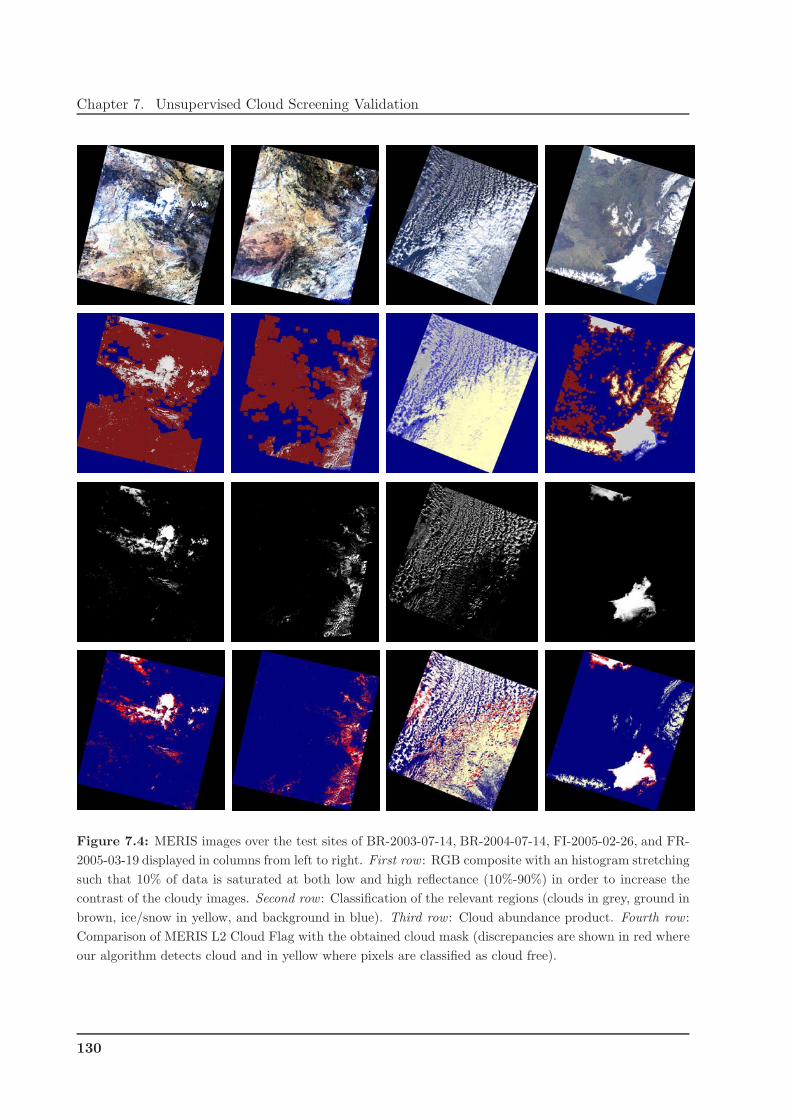
Chapter 7. Unsupervised Cloud Screening Validation
Figure 7.4: MERIS images over the test sites of BR-2003-07-14, BR-2004-07-14, FI-2005-02-26, and FR-
2005-03-19 displayed in columns from left to right. First row : RGB composite with an histogram stretching
such that 10% of data is saturated at both low and high reflectance (10%-90%) in order to increase the
contrast of the cloudy images. Second row : Classification of the relevant regions (clouds in grey, ground in
brown, ice/snow in yellow, and background in blue). Third row : Cloud abundance product. Fourth row :
Comparison of MERIS L2 Cloud Flag with the obtained cloud mask (discrepancies are shown in red where
our algorithm detects cloud and in yellow where pixels are classified as cloud free).
130

7.3. Comparison with MERIS Standard Products
analyst. Incoming radiance from transparent cirrus clouds is mostly affected by the surface
contribution, and it ranges from very low to extremely high values depending on whether cirrus
cloud is over water or ice, respectively. However, the highest altitude clouds in the atmosphere are
cirrus clouds located at altitudes between 5 and 14 km (cf. section 2.1). Despite the variability
of the spectral behavior, the atmospheric features allow us to cluster transparent cirrus clouds
correctly. Summarizing, the use of the oxygen-A absorption allows thick and high/middle-level
clouds to be detected unambiguously. Very low level clouds, very thin cirrus clouds and broken
clouds could be undetected when using only the oxygen feature, but its combined use with surface
reflectance features solves these problems to a great extent. Finally, although the water vapor
absorption feature is less accurate than the oxygen feature for cloud height estimations, it provides
an alternative independent estimation. Besides, it is extremely useful to discriminate clouds from
ice/snow covers due to the incipient absorption of these types of covers in the NIR region above
900 nm (Gao et al., 1998).
7.3 Comparison with MERIS Standard Products
One of the motivations to propose the presented cloud screening algorithm is to solve some
critical problems where the operational MERIS L2 algorithm shows clear deficiencies, as reported
by the user community elsewhere (Ramon et al., 2003; Brockmann, 2006), and by the MERIS
Quality Working Group (MERIS Quality Working Group, 2006). For this reason, we illustrate
the proposed methodology in different scenarios presenting critical cloud screening problems, and
compare it to the MERIS L2 flag solution (cf. section 2.4.1).
Images in the last row of Fig. 7.4 show a comparison of MERIS L2 Cloud Flag with the
results obtained by our algorithm. Pixels where both algorithms agree are depicted in white for
the cloudy pixels and in blue for the cloud free pixels. The agreement between both methods
is shown in Table 7.1 on the basis of the confusion matrices, which are expressed in terms of
percentage of pixels in each image, and the overall accuracy (OA) and estimated kappa statistic1
(κ) derived from them. Although overall agreement between both classifications is good enough
for most of these images, the low values of kappa indicate that significant differences between
methods exist. These differences can be better analyzed looking at the confusion matrices and
comparison maps in Fig. 7.4. From these results, two main discrepancies are found. On the one
hand, pixels classified as cloudy pixels (C) by our method but not by the MERIS flag (C) are
plotted in red, showing a good agreement with cloud borders. Therefore, one can assume that
the proposed method provides better recognition in cloud borders and in small and thin clouds,
which is the situation in the images acquired over Spain. On the other hand, discrepancy pixels
1The use of estimated kappa statistics, κ, is more appropriate than the overall accuracy for testing whether
agreement for both binary cloud classifiers exceeds chance levels (Congalton and Green, 1999). A value of κ = 1
means complete agreement and κ ≤ 0 reflects no agreement. Following this criterion, a classification can be
considered ‘good’ for κ > 0.8 and ‘poor’ for κ < 0.7.
131
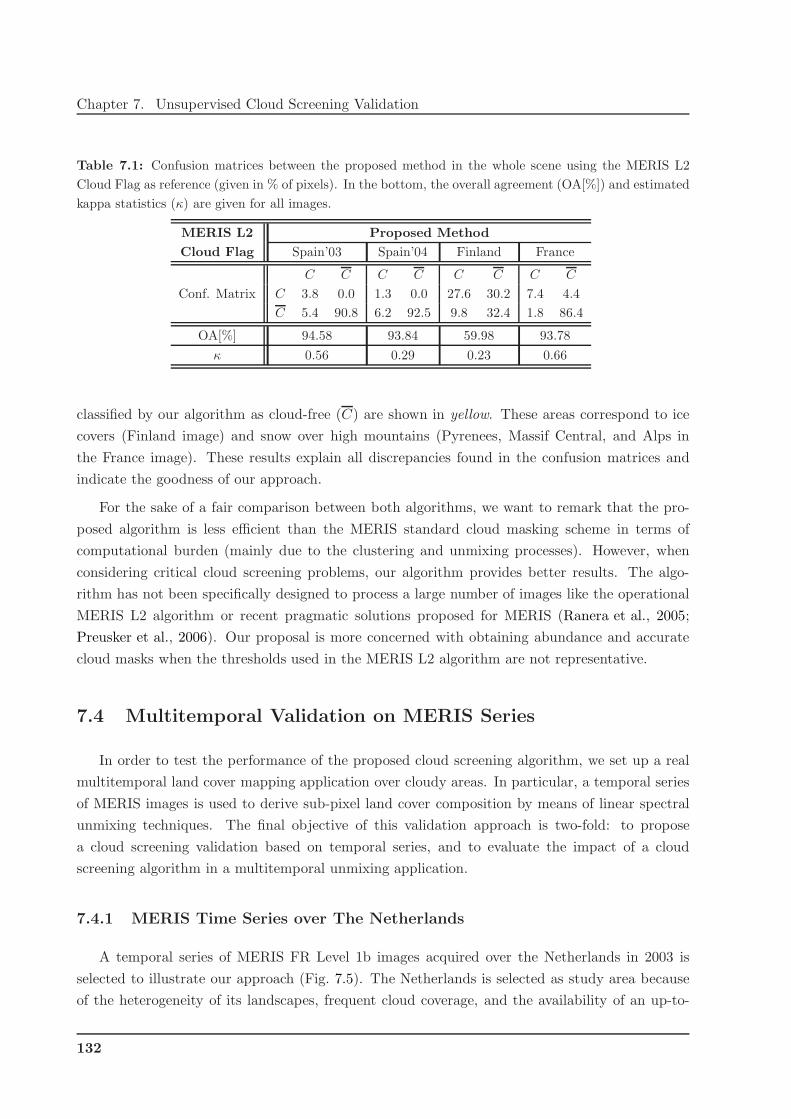
Chapter 7. Unsupervised Cloud Screening Validation
Table 7.1: Confusion matrices between the proposed method in the whole scene using the MERIS L2
Cloud Flag as reference (given in % of pixels). In the bottom, the overall agreement (OA[%]) and estimated
kappa statistics (κ) are given for all images.
MERIS L2 Proposed Method
Cloud Flag Spain’03 Spain’04 Finland France
C C C C C C C C
Conf. Matrix C 3.8 0.0 1.3 0.0 27.6 30.2 7.4 4.4
C 5.4 90.8 6.2 92.5 9.8 32.4 1.8 86.4
OA[%] 94.58 93.84 59.98 93.78
κ 0.56 0.29 0.23 0.66
classified by our algorithm as cloud-free (C) are shown in yellow. These areas correspond to ice
covers (Finland image) and snow over high mountains (Pyrenees, Massif Central, and Alps in
the France image). These results explain all discrepancies found in the confusion matrices and
indicate the goodness of our approach.
For the sake of a fair comparison between both algorithms, we want to remark that the pro-
posed algorithm is less efficient than the MERIS standard cloud masking scheme in terms of
computational burden (mainly due to the clustering and unmixing processes). However, when
considering critical cloud screening problems, our algorithm provides better results. The algo-
rithm has not been specifically designed to process a large number of images like the operational
MERIS L2 algorithm or recent pragmatic solutions proposed for MERIS (Ranera et al., 2005;
Preusker et al., 2006). Our proposal is more concerned with obtaining abundance and accurate
cloud masks when the thresholds used in the MERIS L2 algorithm are not representative.
7.4 Multitemporal Validation on MERIS Series
In order to test the performance of the proposed cloud screening algorithm, we set up a real
multitemporal land cover mapping application over cloudy areas. In particular, a temporal series
of MERIS images is used to derive sub-pixel land cover composition by means of linear spectral
unmixing techniques. The final objective of this validation approach is two-fold: to propose
a cloud screening validation based on temporal series, and to evaluate the impact of a cloud
screening algorithm in a multitemporal unmixing application.
7.4.1 MERIS Time Series over The Netherlands
A temporal series of MERIS FR Level 1b images acquired over the Netherlands in 2003 is
selected to illustrate our approach (Fig. 7.5). The Netherlands is selected as study area because
of the heterogeneity of its landscapes, frequent cloud coverage, and the availability of an up-to-
132

7.4. Multitemporal Validation on MERIS Series
(a) February 18th† (b) April 16th†‡ (c) April 22nd‡ (d) April 23rd (e) May 28th
(f) May 31st† (g) June 6th (h) June 16th (i) July 8th‡ (j) July 14th†‡
(k) August 6th† (l) August 9th (m) August 12th (n) October 15th† (o) December 8th†
† Dates selected for the multitemporal unmixing in the multitemporal land cover mapping application,
which are chosen throughout the year according to its low cloud coverage.
‡ Pairs of cloudy and cloud-free dates used to validate the cloud screening algorithm.
Figure 7.5: Coregistered MERIS FR L1b temporal series acquired over The Netherlands in 2003.
date high spatial resolution land use database. The availability of this high resolution land use
map over The Netherlands is really convenient because it can be used to validate the subpixel
classification results provided by the unmixing, but also as an input of the validation methodology
in order to improve the accuracy of the cloud screening validation.
Most of the acquisition dates of the temporal series presented extensive clouded areas. There-
fore, the selected dates for the multitemporal unmixing are chosen according to two criteria: (i)
to maximize the number of cloud free pixels in each scene and (ii) to get, at least, one image
per month so that the vegetation phenological cycle is fully captured. Unfortunately, no suitable
MERIS FR scene was found for the months of January, March, June, September, and November.
Therefore, an uneven temporal series of seven images is considered for the unmixing: February
18th, April 16th, May 31st, July 14th, August 6th, October 15th, and December 8th. In addition,
images of the 22nd of April and the 8th of July are only used to validate the cloud screening
algorithm. These dates were the closest clouded dates to the 16th of April and 14th of July,
respectively, and thus are needed in order to set up pairs of cloudy and cloud-free images (marked
133
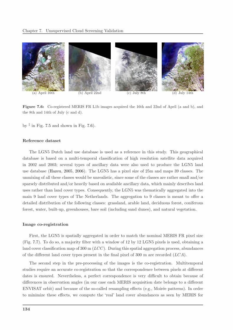
Chapter 7. Unsupervised Cloud Screening Validation
(a) April 16th (b) April 22nd (c) July 8th (d) July 14th
Figure 7.6: Co-registered MERIS FR L1b images acquired the 16th and 22nd of April (a and b), and
the 8th and 14th of July (c and d).
by ‡ in Fig. 7.5 and shown in Fig. 7.6).
Reference dataset
The LGN5 Dutch land use database is used as a reference in this study. This geographical
database is based on a multi-temporal classification of high resolution satellite data acquired
in 2002 and 2003; several types of ancillary data were also used to produce the LGN5 land
use database (Hazeu, 2005, 2006). The LGN5 has a pixel size of 25m and maps 39 classes. The
unmixing of all these classes would be unrealistic, since some of the classes are rather small and/or
sparsely distributed and/or heavily based on available ancillary data, which mainly describes land
uses rather than land cover types. Consequently, the LGN5 was thematically aggregated into the
main 9 land cover types of The Netherlands. The aggregation to 9 classes is meant to offer a
detailed distribution of the following classes: grassland, arable land, deciduous forest, coniferous
forest, water, built-up, greenhouses, bare soil (including sand dunes), and natural vegetation.
Image co-registration
First, the LGN5 is spatially aggregated in order to match the nominal MERIS FR pixel size
(Fig. 7.7). To do so, a majority filter with a window of 12 by 12 LGN5 pixels is used, obtaining a
land cover classification map of 300 m (LCC). During this spatial aggregation process, abundances
of the different land cover types present in the final pixel of 300 m are recorded (LCA).
The second step in the pre-processing of the images is the co-registration. Multitemporal
studies require an accurate co-registration so that the correspondence between pixels at different
dates is ensured. Nevertheless, a perfect correspondence is very difficult to obtain because of
differences in observation angles (in our case each MERIS acquisition date belongs to a different
ENVISAT orbit) and because of the so-called resampling effects (e.g., Moiree patterns). In order
to minimize these effects, we compute the ‘real’ land cover abundances as seen by MERIS for
134
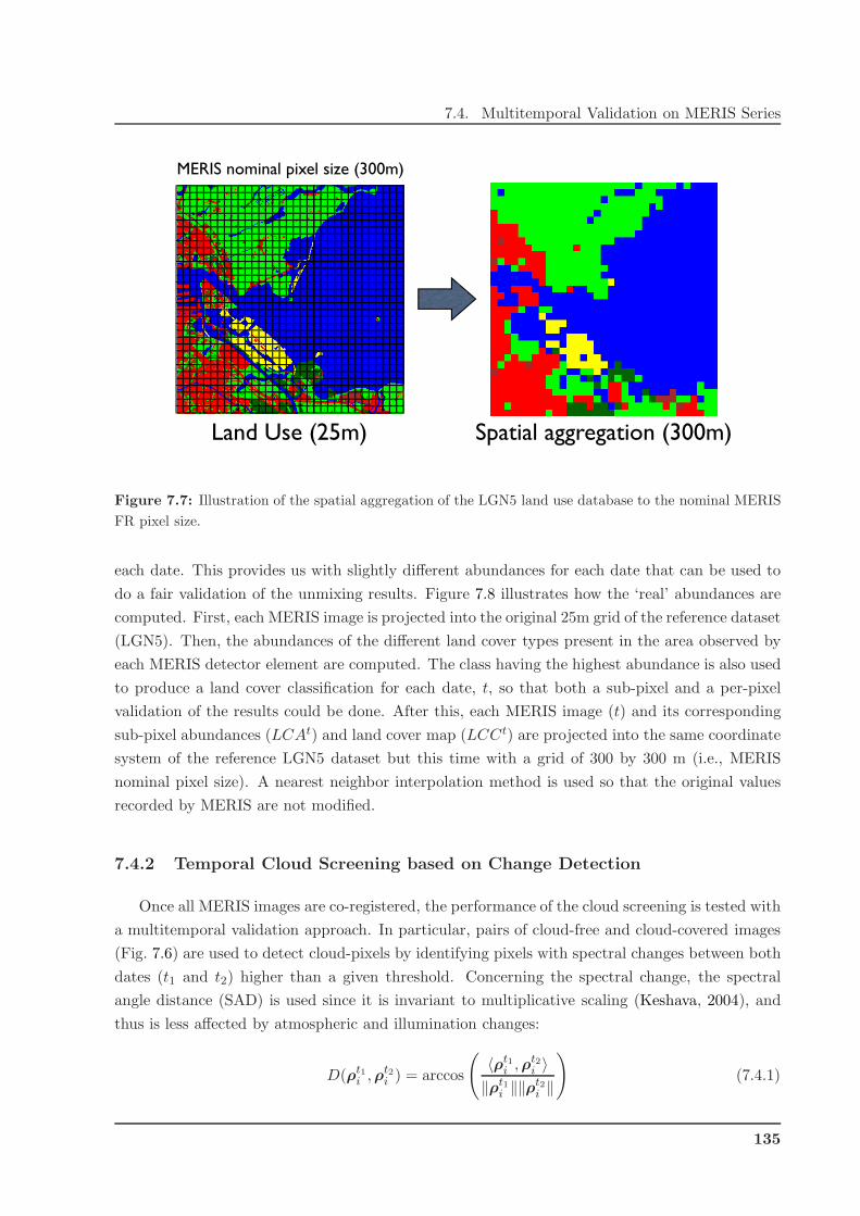
7.4. Multitemporal Validation on MERIS Series
Land Use (25m) Spatial aggregation (300m)
MERIS nominal pixel size (300m)
Figure 7.7: Illustration of the spatial aggregation of the LGN5 land use database to the nominal MERIS
FR pixel size.
each date. This provides us with slightly different abundances for each date that can be used to
do a fair validation of the unmixing results. Figure 7.8 illustrates how the ‘real’ abundances are
computed. First, each MERIS image is projected into the original 25m grid of the reference dataset
(LGN5). Then, the abundances of the different land cover types present in the area observed by
each MERIS detector element are computed. The class having the highest abundance is also used
to produce a land cover classification for each date, t, so that both a sub-pixel and a per-pixel
validation of the results could be done. After this, each MERIS image (t) and its corresponding
sub-pixel abundances (LCAt) and land cover map (LCCt) are projected into the same coordinate
system of the reference LGN5 dataset but this time with a grid of 300 by 300 m (i.e., MERIS
nominal pixel size). A nearest neighbor interpolation method is used so that the original values
recorded by MERIS are not modified.
7.4.2 Temporal Cloud Screening based on Change Detection
Once all MERIS images are co-registered, the performance of the cloud screening is tested with
a multitemporal validation approach. In particular, pairs of cloud-free and cloud-covered images
(Fig. 7.6) are used to detect cloud-pixels by identifying pixels with spectral changes between both
dates (t1 and t2) higher than a given threshold. Concerning the spectral change, the spectral
angle distance (SAD) is used since it is invariant to multiplicative scaling (Keshava, 2004), and
thus is less affected by atmospheric and illumination changes:
D(ρt1i ,ρ
t2i ) = arccos
(
〈ρt1i ,ρ
t2i 〉
‖ρt1i ‖‖ρt2
i ‖
)
(7.4.1)
135

Chapter 7. Unsupervised Cloud Screening Validation
Orbit1 Orbit2
Mask out
abundance
differences
>10%
date1
date2
Figure 7.8: Illustration of the projection and spatial aggregation of the LGN5 land use database to the
actual area observed by the MERIS pixels depending on the observation angles from the given orbit.
where ρt1i and ρt2
i represent the spectra of a given pixel location i for dates t1 and t2, respectively;
〈·, ·〉 is the dot product operator; and ‖ · ‖ is the squared norm. Image pairs are selected to be
close in time in order to avoid spectral changes due to temporal evolution of the surface. However,
images with only three or six days of difference are taken from different orbits and thus present
a significant variation in the viewing angles. Although images are co-registered and a one-to-one
correspondence between the pixels of the two dates can be found, the area observed at each date is
not exactly the same. If the land cover types present in the observed areas change from one date
to the other, then the spatial shift can produce significant spectral changes between ρt1i and ρt2
i .
In consequence, pixels with significant changes in composition, i.e. differences between LCAt1
and LCAt2 derived from de LGN5 higher than 10%, are masked out in the multitemporal cloud
screening validation (Fig. 7.8).
Cloud screening results
A hard cloud mask is obtained for each date t by applying the same threshold of 0.05 to
the cloud abundance product maps ϑt of the proposed algorithm, which are shown in Fig. 7.9.
Since no ground truth indicating cloudy pixels can be generated for all dates, we first analyze the
performance of the proposed method by visual inspection. The analysis of the results showed an
excellent cloud screening performance even in thin clouds and cloud borders. The only exception
is a small amount of pixels belonging to the classes greenhouses (sun glint on glass roofs) and
bare soil (sand dunes). These pixels were identified as clouds because these classes have similar
136
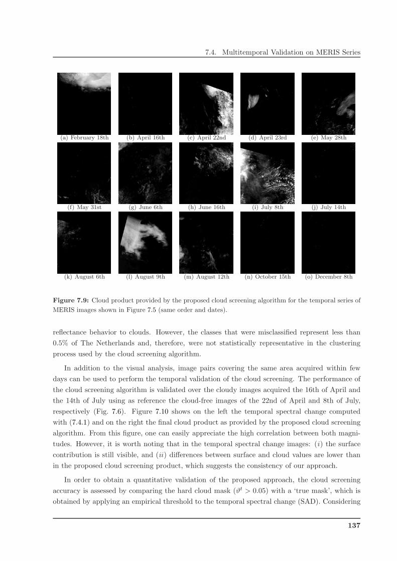
7.4. Multitemporal Validation on MERIS Series
(a) February 18th (b) April 16th (c) April 22nd (d) April 23rd (e) May 28th
(f) May 31st (g) June 6th (h) June 16th (i) July 8th (j) July 14th
(k) August 6th (l) August 9th (m) August 12th (n) October 15th (o) December 8th
Figure 7.9: Cloud product provided by the proposed cloud screening algorithm for the temporal series of
MERIS images shown in Figure 7.5 (same order and dates).
reflectance behavior to clouds. However, the classes that were misclassified represent less than
0.5% of The Netherlands and, therefore, were not statistically representative in the clustering
process used by the cloud screening algorithm.
In addition to the visual analysis, image pairs covering the same area acquired within few
days can be used to perform the temporal validation of the cloud screening. The performance of
the cloud screening algorithm is validated over the cloudy images acquired the 16th of April and
the 14th of July using as reference the cloud-free images of the 22nd of April and 8th of July,
respectively (Fig. 7.6). Figure 7.10 shows on the left the temporal spectral change computed
with (7.4.1) and on the right the final cloud product as provided by the proposed cloud screening
algorithm. From this figure, one can easily appreciate the high correlation between both magni-
tudes. However, it is worth noting that in the temporal spectral change images: (i) the surface
contribution is still visible, and (ii) differences between surface and cloud values are lower than
in the proposed cloud screening product, which suggests the consistency of our approach.
In order to obtain a quantitative validation of the proposed approach, the cloud screening
accuracy is assessed by comparing the hard cloud mask (ϑt > 0.05) with a ‘true mask’, which is
obtained by applying an empirical threshold to the temporal spectral change (SAD). Considering
137
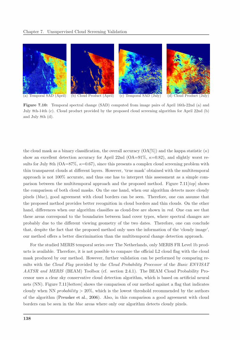
Chapter 7. Unsupervised Cloud Screening Validation
(a) Temporal SAD (April) (b) Cloud Product (April) (c) Temporal SAD (July) (d) Cloud Product (July)
Figure 7.10: Temporal spectral change (SAD) computed from image pairs of April 16th-22nd (a) and
July 8th-14th (c). Cloud product provided by the proposed cloud screening algorithm for April 22nd (b)
and July 8th (d).
the cloud mask as a binary classification, the overall accuracy (OA[%]) and the kappa statistic (κ)
show an excellent detection accuracy for April 22nd (OA=91%, κ=0.82), and slightly worst re-
sults for July 8th (OA=87%, κ=0.67), since this presents a complex cloud screening problem with
thin transparent clouds at different layers. However, ‘true mask’ obtained with the multitemporal
approach is not 100% accurate, and thus one has to interpret this assessment as a simple com-
parison between the multitemporal approach and the proposed method. Figure 7.11[top] shows
the comparison of both cloud masks. On the one hand, when our algorithm detects more cloudy
pixels (blue), good agreement with cloud borders can be seen. Therefore, one can assume that
the proposed method provides better recognition in cloud borders and thin clouds. On the other
hand, differences when our algorithm classifies as cloud-free are shown in red. One can see that
these areas correspond to the boundaries between land cover types, where spectral changes are
probably due to the different viewing geometry of the two dates. Therefore, one can conclude
that, despite the fact that the proposed method only uses the information of the ‘cloudy image’,
our method offers a better discrimination than the multitemporal change detection approach.
For the studied MERIS temporal series over The Netherlands, only MERIS FR Level 1b prod-
ucts is available. Therefore, it is not possible to compare the official L2 cloud flag with the cloud
mask produced by our method. However, further validation can be performed by comparing re-
sults with the Cloud Flag provided by the Cloud Probability Processor of the Basic ENVISAT
AATSR and MERIS (BEAM) Toolbox (cf. section 2.4.1). The BEAM Cloud Probability Pro-
cessor uses a clear sky conservative cloud detection algorithm, which is based on artificial neural
nets (NN). Figure 7.11[bottom] shows the comparison of our method against a flag that indicates
cloudy when NN probability > 20%, which is the lowest threshold recommended by the authors
of the algorithm (Preusker et al., 2006). Also, in this comparison a good agreement with cloud
borders can be seen in the blue areas where only our algorithm detects cloudy pixels.
138

7.4. Multitemporal Validation on MERIS Series
April 22nd July 8th
Multitem
por
alC
loud
Fla
g
0:Background
1:Land / Land
2:Cloud / Land
3:Land / Cloud
4:Cloud / CloudB
EA
MC
loud
Fla
g
0:Background
1:Land / Land
2:Cloud / Land
3:Land / Cloud
4:Cloud / Cloud
Figure 7.11: Comparison of the obtained cloud mask against the multitemporal cloud flag (top) and
against the BEAM Cloud Probability Processor Flag (bottom) for the images of April 22nd (left) and July
8th (right). Discrepancies between methods are shown in blue when our algorithm detects cloud and in
red when pixels are classified as cloud-free.
7.4.3 Spectral Unmixing of Multitemporal Series
An indirect procedure to test cloud screening performance consists in analyzing its effect in a
real application. Undetected clouds are one of the most significant sources of error in both sea and
land cover biophysical parameter retrieval. For example, in a land use classification application
based on spectral unmixing of multitemporal series, undetected clouds can hamper the selection
of endmembers and seriously affect the quality of the unmixing of cloud contaminated pixels.
Therefore, cloud screening is needed to remove all the cloudy pixels from the final analysis. As a
consequence, an accurate cloud screening should significantly increase the classification accuracy.
The algorithm used to perform the spectral unmixing is the fully constrained linear spectral
unmixing (Heinz and Chang, 2001) presented in section 5.3.1, which can be applied to each MERIS
139
Chapter 7. Unsupervised Cloud Screening Validation
image (mono-temporal case) as well as to a multitemporal composite (stacked approach) of all
the MERIS images. The FCLSU guarantees a physical interpretation of the results, and can be
formalized as follows:
ρti(λb) =
Q∑
q=1
mtq(λi)a
tiq + ε (7.4.2)
subject to 0 ≤ atiq ≤ 1 and
∑
q atiq = 1; where ρt
i(λb) is pixel i value for band b at date t, Q
represents the number of class endmembers, mtq, that are being unmixed, being the coefficients
of this combination, atiq, the unmixing coefficients, which can be interpreted as the abundance
fractions of materials or classes in a pixel. Finally, the term ε represents the residual error per
band, assumed constant for all bands.
In the multitemporal case, the spectral signature of each class, mq, is the stacked vector
formed by the class endmember of all dates, mq = [mt1q ,m
t2q , . . . ], and the pixel to be unmixed,
ρi, is the stacked vector ρi = [ρt1i ,ρ
t2i , . . . ]. Now, (7.4.2) can be expressed in a matrix form as
ρi = M · ai + ε, where the spectral signatures of materials, mq, are expressed in the columns of
matrix M.
Multitemporal unmixing results
After applying the cloud screening algorithm to all the selected images, identified cloud con-
taminated pixels are masked out and the spectral unmixing is carried out. Figure 7.12(a) shows
the spectral signature of the endmembers for the seven dates selected in this study. Grassland
presents the highest NIR reflectance all year around. During the months of May, July, and August
the endmember of deciduous forest also shows high reflectance (high greening of vegetation). The
rest of the vegetated classes appear to have a very similar spectral signature. High confusion is,
therefore, expected among these classes. On the one hand, in the spectral unmixing of one image,
the land cover abundances cannot be obtained over clouded areas or outside the field of view of
the sensor. On the other hand, in the multitemporal unmixing, each pixel is formed as the stacked
vector of the spectra for all the available dates. This allows us to obtain the abundance fractions
in all the pixels of the studied area, but the number of dates used in multitemporal unmixing is
pixel dependent since each pixel is unmixed with the maximum number of valid cloud free dates.
This means that the quality of the unmixing is also pixel-dependent and that, whenever critical
(phenological) dates are missing for a number of pixels (e.g. clouded areas), the accuracy of the
results on those pixels (areas) might be lower. Figure 7.12(b) shows the number of usable dates for
each pixel after masking out the clouds and cloud borders. It should be noted that the northern
and south-eastern parts of The Netherlands have less usable pixels than the rest of the country.
This is not only because of the cloud coverage but also because some of the MERIS FR images
did not cover the whole of The Netherlands.
A detailed description of the multitemporal spectral unmixing and the obtained results is given
in Gomez-Chova et al. (2006f). Here, we have only focused on the impact of cloud screening in
140

7.4. Multitemporal Validation on MERIS Series
Jan Feb Mar Apr May Jun Jul Aug Sep Oct Nov Dec0
0.1
0.2
0.3
0.4
0.5
TO
A R
efl
ect
an
ce
Grassland
Arable land
Greenhouses
Deciduous forest
Coniferous forest
Water
Built−up
Bare soil
Natural vegetation
(a) (b)
Figure 7.12: (a) Pure temporal endmembers selected from the multitemporal dataset for each land cover
class. (b) Per-pixel number of usable dates.
(a)
0:No data
1:Grassland
2:Arable land
3:Greenhouses
4:Deciduous forest
5:Coniferous forest
6:Water
7:Built up
8:Bare soil
9:Natural vegetation
(b)
Figure 7.13: (a) Classification obtained from the multitemporal unmixing abundances. (b) LGN5 resam-
pled to 9 classes and 300 m used as ground truth.
the multitemporal unmixing. However, in the following, we summarize the main unmixing results
in order to show the importance of an accurate cloud screening. The unmixed abundances for
each date, ati, and the multitemporal approach, ai, are compared to the abundances computed
during the spatial aggregation of the LGN5 database, LCA. Then, the classification obtained
from the abundances (Fig. 7.13) is used to compute the overall classification accuracy and the
kappa statistic using the LCC as ground truth (Table 7.2). As expected, the multitemporal ap-
proach yielded the highest classification results, since adding the temporal evolution (phenology)
simplifies the discrimination of spectrally similar land cover types. However, the difference be-
tween the classification results of the best (monotemporal) image [April] and the multitemporal
approach is not very large. These errors in the multitemporal case should be produced by the
within class heterogeneity (land covers with different phenology mixed in one class, e.g. arable
141

Chapter 7. Unsupervised Cloud Screening Validation
Table 7.2: Performance of the land cover classification using the FCLU at per pixel scale (overall accuracy,
OA[%], and kappa statistics, κ) for each single date and the multitemporal series.
Data Feb Apr May Jul Aug Oct Dec Multitemporal
Kappa 0.36 0.49 0.39 0.45 0.36 0.37 0.35 0.52
OA[%] 46.44 58.58 50.33 56.10 46.81 49.88 47.55 62.29
land class) or by the procedure used to elaborate the LGN5 used as ground truth. In conclusion,
the accurate cloud screening performed by the proposed algorithm enables a more efficient use of
MERIS images.
7.5 The Cloud Abundance Product
Finally, one of the requirements imposed to the proposed cloud screening methodology was
to provide information about the contribution of clouds to the spectra of image pixels (for both
transparent clouds or subpixel coverage situations). This type of information may be very useful
for the users in order to decide what is a cloud depending on the application requirements or
image conditions. In this work, we classify as cloud all pixels presenting values higher than 0.05
in the obtained cloud abundance product. It should be noted that this threshold is the same for
all images analyzed in order to demonstrate the general applicability of the method. This value is
so low because the classification probability makes almost zero the cloud abundance product for
all the cloud-free pixels. However, if the user is not interested in excluding pixels slightly affected
by clouds in a given application, the threshold value can be increased.
In order to show the potential of the cloud abundance product, Fig. 7.14 shows the histograms
of the obtained values of posterior probability hiC (dark) and cloud product ϑi (white) for all
images. The smooth distribution of ϑi values differs to a great extent from the output of the
probabilistic classifier, which has no physical meaning and is usually unevenly distributed around
zero and one.
Finally, we can also validate our abundance product against the cloud probability provided
by the Cloud Probability Processor implemented in the BEAM Toolbox, which is the most similar
cloud product available for MERIS data. Figure 7.15 shows the histograms of the proposed
cloud product (white) and the BEAM cloud probability (dark) values. Again, our algorithm
provides a smoother distribution of ϑ values, which differs to a great extent from the output of
the probabilistic NN classifier that is concentrated around one.
142

7.5. The Cloud Abundance Product
0 0.2 0.4 0.6 0.8 1posterior probability h
kC and cloud product φ
k values ∈ [0,1]
num
ber
of s
ampl
es
(a) BR-2003-07-14
0 0.2 0.4 0.6 0.8 1posterior probability h
kC and cloud product φ
k values ∈ [0,1]
num
ber
of s
ampl
es
(b) BR-2004-07-14
0 0.2 0.4 0.6 0.8 1posterior probability h
kC and cloud product φ
k values ∈ [0,1]
num
ber
of s
ampl
es
(c) FI-2005-02-26
0 0.2 0.4 0.6 0.8 1posterior probability h
kC and cloud product φ
k values ∈ [0,1]
num
ber
of s
ampl
es
(d) FR-2005-03-19
Figure 7.14: Histogram of the posterior probability hiC (dark) and cloud product ϑi (white) values for
the images of BR-2003-07-14 (a), BR-2004-07-14 (b), FI-2005-02-26 (c), and FR-2005-03-19 (d). Extreme
low and high values have been excluded for a proper visualization.
0 0.2 0.4 0.6 0.8 1cloud product values ∈ [0,1]
num
ber
of sam
ple
s
(a) April 22nd
0 0.2 0.4 0.6 0.8 1cloud product values ∈ [0,1]
num
ber
of sam
ple
s
(b) July 8th
Figure 7.15: Histogram of the proposed cloud product (white) and the BEAM cloud probability (dark)
values for the images of April 22nd (a) and July 8th (b). Extreme low and high values have been excluded
for a proper visualization.
143

Chapter 7. Unsupervised Cloud Screening Validation
144
Chapter 8
Semi-supervised Cloud Screening
Validation
The user-driven approach proposed in Chapter 5 has shown an excellent cloud screening
performance in the results as presented in Chapter 7. However, this approach is best suited
to case studies due to its computational cost and the optional interaction of the user during
the labeling process. In operational cloud screening applications, methods that automatically
and accurately classify clouds are mandatory. Therefore, supervised or semi-supervised methods
should be more appropriate due to their typically enhanced performance. This chapter describes
the cloud screening results obtained with the novel kernel methods presented in Chapter 6. All
these methods are supervised or semi-supervised classifiers, and thus they require a representative
set of labeled samples to train and validate the models.
As we mentioned in previous chapters, in a real cloud screening classification problem, no
simultaneous independent assessment measurement of cloud presence at the same image spatial
resolution is usually available. Therefore, it is not easy to obtain the true label (cloud or cloud-
free) for the image pixels. In the case of MERIS images, only two cloud mask products (obtained
in an operational basis) can be used as a reference in order to compare the results of the proposed
cloud screening approaches. These two cloud masks, which are derived directly from the MERIS
image, are the official MERIS L2 Cloud Flag and the BEAM Cloud Probability Processor Flag
that provides a more accurate cloud mask than the official product. However, results presented
in Chapter 7 revealed that both methods have deficiencies. In fact, the analysis carried out in
Chapter 7 showed that the method based on unsupervised clustering proposed in Chapter 5 is
the most accurate cloud screening method, especially when the labeling of the found clusters is
done by the user (user-driven approach). Therefore, the true labels and true maps used to train
and validate the classifiers presented in this chapter are based on the proposed cloud abundance
product (see section 5.3.3).

Chapter 8. Semi-supervised Cloud Screening Validation
8.1 Experimental Setup
In a real cloud screening classification problem, it is difficult to collect a statistically significant
number of ground-truth samples to define a complete training set for developing robust supervised
classifiers. This usually leads to a poor representation of the problem by the training set that
can induce the so-called sample selection bias problem, i.e. the available training set is not repre-
sentative enough of the test set. For this reason, the proposed kernel methods are benchmarked
in two different conditions: (1) few labeled training samples are available for characterizing the
image to be classified; and (2) no labeled training samples are available for the test image to be
classified. In the latter case, training data extracted from other images modeling similar problems
are exploited to develop the classifiers. In both situations, unlabeled samples of the test image
can be jointly used with the available training samples to increase the reliability and accuracy of
the classifier. In this context, two scenarios are further considered: labeled and unlabeled training
samples might belong to the image to be classified, or to different images coming from different
locations and acquired in eventually very different conditions. The most realistic situation in op-
erational remote sensing applications is, nevertheless, to obtain the labeled samples from previous
images and the unlabeled samples from the image to be classified. Summarizing, two challenging
scenarios are considered:
Single-Image Approach. In these experiments, labeled and unlabeled training samples belong
to the image to be classified. This is a common scenario in remote sensing, when a single
image is available or is going to be analyzed, and the training set is built by labeling some
representative samples, usually by an expert or by using additional ground measurements.
In this case, both the training and test data come from the same marginal distribution,
and thus the classifiers are not affected by the sample selection bias problem. We call this
procedure the single-image approach.
Image-Fold Approach. A completely different (and more realistic) situation is to obtain the
labeled training samples from previous images or from physical model simulations, and
then apply the developed models to a test set, which usually consists of several images. In
this case, the available training set can be not representative enough for the test (sample
selection bias problem) and the unlabeled samples from the image to be classified should
help to improve the classification accuracy. In order to analyze this scenario, in this chapter,
we carry out some experiments where classifiers are trained using both labeled samples from
the N − 1 out of N available images, and unlabeled samples from the image to be classified.
We call this procedure the image-fold approach (see Fig. 8.1).
Table 8.1 describes the data sets used to develop the kernel classifiers and the experimental
setup followed to obtain the cloud screening results. The input features used by all the methods
are extracted from the MERIS L1b images, as described in Chapter 4. The labels of the image
pixels are obtained from the cloud abundance product (cf. section 5.3.3), which has been analyzed
146

8.1. Experimental Setup
I1
Training Set
Test SetI2 I3 I4 I5
Classifier
I1
Training Set
Test SetI2 I3 I4 I5
Classifier
I1
Training Set
Test SetI2 I3 I4 I5
Classifier
I1
Training Set
Test SetI2 I3 I4 I5
Classifier
I1
Training Set
Test SetI2 I3 I4 I5
Classifier
Figure 8.1: Image-fold approach followed in the experiments in order to induce the sample selection
bias in the training process. Classifiers are trained using both labeled samples from the N − 1 out of N
available images, and unlabeled samples from the image to be classified. The scheme depicts a 5-image-fold
approach, where a different classifier is trained for each image. Finally, classification results on test are
averaged for the 5 images to evaluate the robustness of the classifiers to the sample selection bias.
147

Chapter 8. Semi-supervised Cloud Screening Validation
Table 8.1: Experimental setup and data used to develop the kernel classifiers and to obtain the cloud
screening results.
Data Sets
Input Features All methods are applied to the vector of extracted features for each pixel:
xi = [fBr,VIS, fBr,NIR, fWh, fO2, fWV]⊤, which correspond to the target spec-
tral brightness in the VIS and NIR, the target spectral whiteness, and the
oxygen and water vapor atmospheric absorptions, respectively.
Labels (yi) Supervised information defining the labels (cloud/cloud-free) of the image
pixels is obtained by applying a threshold of 0.05 to the cloud abundance
product (cf. section 5.3.3), presented in Chapter 7: yi = sgn(ϑi − 0.05).
Samples (xi) 10000 labeled samples covering the full range of ϑ values are selected from
each image. These samples are used to generate the different training and
validation sets used to develop and compare the models.
Clusters (ωk) The EM algorithm is applied to each image in order to obtain the clus-
ters present in the image, together with the cluster membership hik, and
assigned cluster hi for each sample xi.
Training Set A given number of samples is used to develop the models during the train-
ing process. For all models, a set of ℓ labeled samples {xi, yi}ℓi=1 is used.
For semi-supervised models, a set of u unlabeled samples {xi}ℓ+ui=ℓ+1 is also
included in the training set. In the later case, we assume that the unla-
beled samples come from the image to be classified, and their labels yi are
unknown, but their cluster membership hi has been obtained. In the exper-
iments, the number of unlabeled samples is fixed to u = 800 and we explore
from ill-posed situations with only 4 labeled samples per class (ℓ = 8) up to
well-posed supervised cases with 200 labeled samples per class (ℓ = 400).
The best model for each experiment is selected by 10-fold cross-validation
over the labeled training samples evaluating the averaged κ statistics.
Validation Set An independent dataset of 5000 labeled samples from the test image is
used to compare the performance of the classifiers. These samples are used
to compute the κ classification accuracy of the different models but not
to tune the free parameters of the models, i.e. validation samples are not
used during the training phase since the best model is selected with the
10-fold cross-validation approach. In addition, in order to avoid skewed
conclusions, we run all experiments for a number of realizations where the
used training samples were randomly selected. Therefore, the validation
results are averaged for 10 realizations in order to measure the robustness
of the methods in the classification.
Test Set The developed classifiers are finally applied to all the pixels of the test
image in order to obtain the classification maps.
148
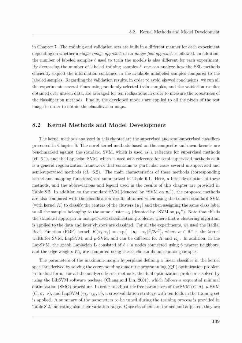
8.2. Kernel Methods and Model Development
in Chapter 7. The training and validation sets are built in a different manner for each experiment
depending on whether a single-image approach or an image-fold approach is followed. In addition,
the number of labeled samples ℓ used to train the models is also different for each experiment.
By decreasing the number of labeled training samples ℓ, one can analyze how the SSL methods
efficiently exploit the information contained in the available unlabeled samples compared to the
labeled samples. Regarding the validation results, in order to avoid skewed conclusions, we run all
the experiments several times using randomly selected train samples, and the validation results,
obtained over unseen data, are averaged for ten realizations in order to measure the robustness of
the classification methods. Finally, the developed models are applied to all the pixels of the test
image in order to obtain the classification maps.
8.2 Kernel Methods and Model Development
The kernel methods analyzed in this chapter are the supervised and semi-supervised classifiers
presented in Chapter 6. The novel kernel methods based on the composite and mean kernels are
benchmarked against the standard SVM, which is used as a reference for supervised methods
(cf. 6.1), and the Laplacian SVM, which is used as a reference for semi-supervised methods as it
is a general regularization framework that contains as particular cases several unsupervised and
semi-supervised methods (cf. 6.2). The main characteristics of these methods (corresponding
kernel and mapping functions) are summarized in Table 6.1. Here, a brief description of these
methods, and the abbreviations and legend used in the results of this chapter are provided in
Table 8.2. In addition to the standard SVM (denoted by “SVM on xi”), the proposed methods
are also compared with the classification results obtained when using the trained standard SVM
(with kernel K) to classify the centers of the clusters (µk) and then assigning the same class label
to all the samples belonging to the same cluster ωk (denoted by “SVM on µk”). Note that this is
the standard approach in unsupervised classification problems, where first a clustering algorithm
is applied to the data and later clusters are classified. For all the experiments, we used the Radial
Basis Function (RBF) kernel, K(xi,xj) = exp(
−‖xi − xj‖2/2σ2)
, where σ ∈ R+ is the kernel
width for SVM, LapSVM, and µ-SVM, and can be different for K and Kµ. In addition, in the
LapSVM, the graph Laplacian L consisted of ℓ + u nodes connected using 6 nearest neighbors,
and the edge weights Wij are computed using the Euclidean distance among samples.
The parameters of the maximum-margin hyperplane defining a linear classifier in the kernel
space are derived by solving the corresponding quadratic programming (QP) optimization problem
in its dual form. For all the analyzed kernel methods, the dual optimization problem is solved by
using the LibSVM software package (Chang and Lin, 2001), which follows a sequential minimal
optimization (SMO) procedure. In order to adjust the free parameters of the SVM (C, σ), µ-SVM
(C, σ, ν), and LapSVM (γL, γM , σ), a cross-validation strategy with ten folds in the training set
is applied. A summary of the parameters to be tuned during the training process is provided in
Table 8.2, indicating also their variation range. Once classifiers are trained and adjusted, they are
149

Chapter 8. Semi-supervised Cloud Screening Validation
Table 8.2: Summary of the analyzed kernel methods and the parameters to be tuned during the training.
Kernel Methods (see Table 6.1)
SVM on xi Kℓ×ℓ SVM trained with the ℓ labeled samples and applied to each
sample xj to obtain its class label: K(xi,xj) = 〈φ(xi),φ(xj)〉.SVM on µk Kℓ×ℓ SVM trained with the ℓ labeled samples but applied to each
cluster center µk in order to obtain its class label that is prop-
agated to all the samples belonging to this cluster: K(xi,µk).
LapSVM Kn×n Laplacian SVM trained with the n = ℓ+u labeled and unlabeled
samples of the training set (see 6.2 for details).
µ-SVM in X KXµ Mean-Map SVM based on the cluster similarity in X , i.e.
computed between the cluster centers µk in the input space:
KXµ = 〈φ(µ1),φ(µ2)〉
KXω Mean-Map SVM combining both the sample similarity and the
cluster similarity in X through composite kernels: KXω = νK+
(1 − ν)KXµ .
µ-SVM in H KHµ Mean-Map SVM based on the cluster similarity in H, i.e. com-
puted between the clusters Sk in the kernel space by using the
mean map: KHµ (S1, S2) =
⟨
φµ(S1),φµ(S2)⟩
.
KHω Mean-Map SVM combining both the sample similarity and the
cluster similarity in H through composite kernels: KHω = νK+
(1 − ν)KHµ .
µs-SVM in H KHµs
Mean-Map SVM based on the cluster similarity in H, i.e. com-
puted between the clusters Sk in the kernel space by using the
soft mean map: KHµs
(S1, S2) =⟨
φµs(S1),φµs
(S2)⟩
.
KHωs
Mean-Map SVM combining both the sample similarity and the
soft cluster similarity in H through composite kernels: KHωs
=
νK + (1 − ν)KHµs
.
Free Parameters
SVMKernel width σ ∈ R
+ of the RBF kernel, K(xi,xj) =
exp(
−‖xi − xj‖2/2σ2)
, was tuned in the range {10−3, . . . , 10}.Regularization parameter C was varied in the range {10−1, . . . , 102}.
LapSVMKernel width σ was varied as in the SVM.
γL and γM were varied in steps of one decade in the range {10−4, . . . , 104}.The graph Laplacian L was computed using 6 neighbors.
µ-SVMKernel width σ and C were varied as in the SVM.
Weight ν was tuned in the range {0.01, . . . , 0.99} for composite kernels.
150
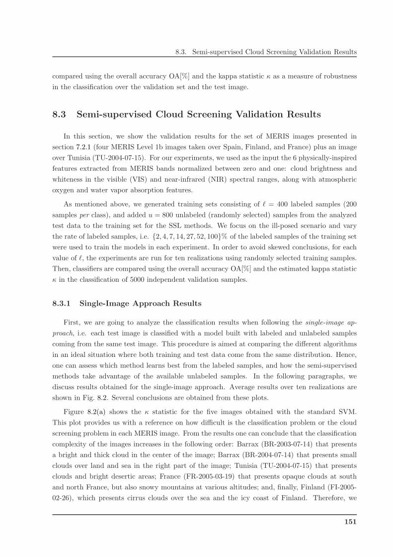
8.3. Semi-supervised Cloud Screening Validation Results
compared using the overall accuracy OA[%] and the kappa statistic κ as a measure of robustness
in the classification over the validation set and the test image.
8.3 Semi-supervised Cloud Screening Validation Results
In this section, we show the validation results for the set of MERIS images presented in
section 7.2.1 (four MERIS Level 1b images taken over Spain, Finland, and France) plus an image
over Tunisia (TU-2004-07-15). For our experiments, we used as the input the 6 physically-inspired
features extracted from MERIS bands normalized between zero and one: cloud brightness and
whiteness in the visible (VIS) and near-infrared (NIR) spectral ranges, along with atmospheric
oxygen and water vapor absorption features.
As mentioned above, we generated training sets consisting of ℓ = 400 labeled samples (200
samples per class), and added u = 800 unlabeled (randomly selected) samples from the analyzed
test data to the training set for the SSL methods. We focus on the ill-posed scenario and vary
the rate of labeled samples, i.e. {2, 4, 7, 14, 27, 52, 100}% of the labeled samples of the training set
were used to train the models in each experiment. In order to avoid skewed conclusions, for each
value of ℓ, the experiments are run for ten realizations using randomly selected training samples.
Then, classifiers are compared using the overall accuracy OA[%] and the estimated kappa statistic
κ in the classification of 5000 independent validation samples.
8.3.1 Single-Image Approach Results
First, we are going to analyze the classification results when following the single-image ap-
proach, i.e. each test image is classified with a model built with labeled and unlabeled samples
coming from the same test image. This procedure is aimed at comparing the different algorithms
in an ideal situation where both training and test data come from the same distribution. Hence,
one can assess which method learns best from the labeled samples, and how the semi-supervised
methods take advantage of the available unlabeled samples. In the following paragraphs, we
discuss results obtained for the single-image approach. Average results over ten realizations are
shown in Fig. 8.2. Several conclusions are obtained from these plots.
Figure 8.2(a) shows the κ statistic for the five images obtained with the standard SVM.
This plot provides us with a reference on how difficult is the classification problem or the cloud
screening problem in each MERIS image. From the results one can conclude that the classification
complexity of the images increases in the following order: Barrax (BR-2003-07-14) that presents
a bright and thick cloud in the center of the image; Barrax (BR-2004-07-14) that presents small
clouds over land and sea in the right part of the image; Tunisia (TU-2004-07-15) that presents
clouds and bright desertic areas; France (FR-2005-03-19) that presents opaque clouds at south
and north France, but also snowy mountains at various altitudes; and, finally, Finland (FI-2005-
02-26), which presents cirrus clouds over the sea and the icy coast of Finland. Therefore, we
151
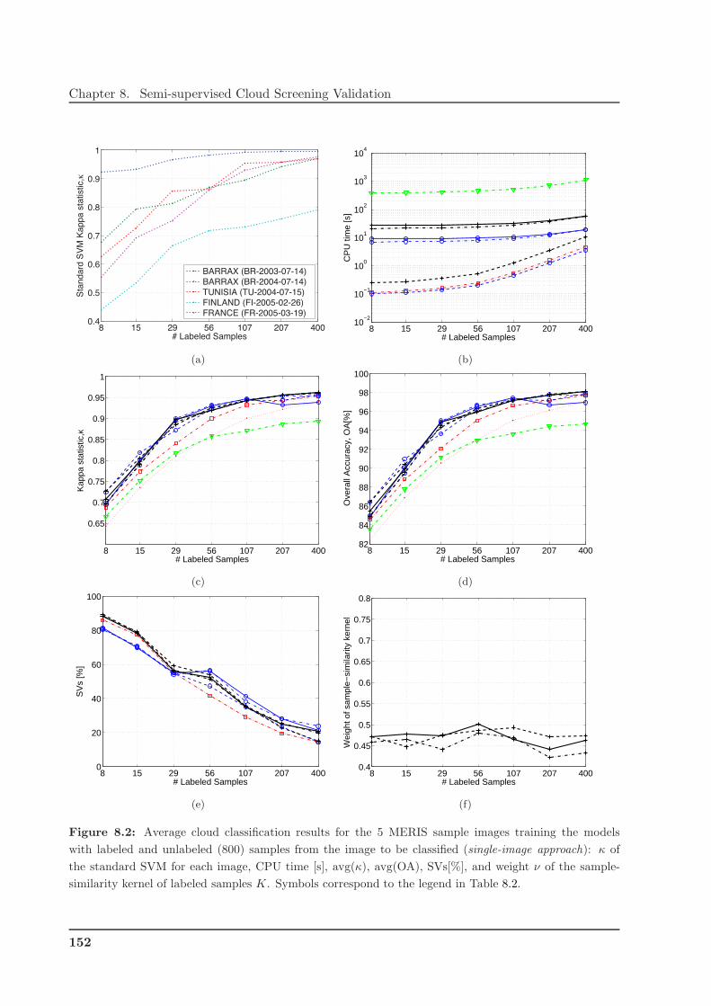
Chapter 8. Semi-supervised Cloud Screening Validation
8 15 29 56 107 207 4000.4
0.5
0.6
0.7
0.8
0.9
1
# Labeled Samples
Sta
nd
ard
SV
M K
ap
pa
sta
tistic,κ
BARRAX (BR-2003-07-14)BARRAX (BR-2004-07-14)TUNISIA (TU-2004-07-15)FINLAND (FI-2005-02-26)FRANCE (FR-2005-03-19)
(a)
8 15 29 56 107 207 40010
−2
10−1
100
101
102
103
104
CP
U ti
me
[s]
# Labeled Samples
(b)
8 15 29 56 107 207 400
0.65
0.7
0.75
0.8
0.85
0.9
0.95
1
Kap
pa s
tatis
tic,κ
# Labeled Samples
(c)
8 15 29 56 107 207 40082
84
86
88
90
92
94
96
98
100
Ove
rall
Acc
urac
y, O
A[%
]
# Labeled Samples
(d)
8 15 29 56 107 207 4000
20
40
60
80
100
SV
s [%
]
# Labeled Samples
(e)
8 15 29 56 107 207 4000.4
0.45
0.5
0.55
0.6
0.65
0.7
0.75
0.8
Wei
ght o
f sam
ple−
sim
ilarit
y ke
rnel
# Labeled Samples
(f)
Figure 8.2: Average cloud classification results for the 5 MERIS sample images training the models
with labeled and unlabeled (800) samples from the image to be classified (single-image approach): κ of
the standard SVM for each image, CPU time [s], avg(κ), avg(OA), SVs[%], and weight ν of the sample-
similarity kernel of labeled samples K. Symbols correspond to the legend in Table 8.2.
152

8.3. Semi-supervised Cloud Screening Validation Results
are including in the experiments both easy cloud screening problems, where few labeled samples
are enough to obtain accurate classifications, and extremely complex cloud screening scenarios,
where a reasonable number of labeled samples is required to correctly detect clouds when using
a standard supervised classifier. In the remaining plots of Fig. 8.2, the results obtained for these
five scenes are averaged in order to discover which method performs best in most of the scenarios.
Figure 8.2(b) shows the average CPU time consumed by each method during the training
phase. All experiments were carried out in a 64-bit dual-core Intel R© XeonTM CPU 2.80GHz
processor under Linux, and all methods are based on MATLAB implementations with a QP/SMO
algorithm programmed in C++ (Chang and Lin, 2001). In this plot, three groups of methods are
easily distinguished. Firstly, the best performance in terms of CPU time is obtained by the
standard SVM and the µ-SVM in X , which only require to compute the kernel matrix for the
labeled samples Kℓ×ℓ. In fact, KXµ method is slightly faster than the SVM since it only computes
the kernel matrix over the cluster centers µk in the input space (KXµ = 〈φ(µ1),φ(µ2)〉) and
the number of clusters c in the image is usually much lower than the number of labeled samples
ℓ. On the other hand, KXω = νK + (1 − ν)KX
µ is slightly slower than these methods since the
weighting parameter ν is also tuned during the training phase. Secondly, the proposed µs-SVM
classifiers in H provide an acceptable performance but are slower than previous methods since, in
order to compute the similarity between clusters in the kernel space KXµ , they have to compute
the kernel matrix for the labeled and unlabeled samples K(ℓ+u)×(ℓ+u). However, this difference
is reduced when the number of labeled samples ℓ approaches the number of unlabeled samples
u = 5000. Again, the weighted versions of the µ-SVM (‘+’ markers) are slower than the versions
based on clusters exclusively (‘◦’ markers) because of the tuning of ν. Finally, LapSVM is around
a thousand times more demanding than SVM in terms of CPU time, and a thousand times more
demanding than µ-SVM. It can be explained because the training of LapSVM models requires
tuning more free parameters than in the SVM case, but the main problem is that a (ℓ+u)×(ℓ+u)
matrix consisting of labeled and unlabeled samples must be inverted.
Figures 8.2(c) and 8.2(d) show the average κ and OA for all the methods. The first conclusion
extracted from the curves is that the proposed µ-SVM method clearly improves the results of the
other methods. The mean kernels classifiers produce better classification results than the reference
provided by the supervised SVM in all cases (note that SVM is a particular case of the µ-SVM
for ν = 1). These results are a consequence of taking into account the distribution of image data
to define the clusters. In consequence, µ-SVM classifiers can be considered as a good trade-off
between computational cost and classification accuracy. In addition, µ-SVM classifiers working
in the kernel space provide slightly better results, supporting the idea that we can find a richer
space H for separating classes. In ill-posed situations, with a low number of labeled samples, the
performance of µ-SVM in H is reversed and µ-SVM in X provide better results. This fact can
be explained since, when working with a low number of labeled samples, v-fold cross-correlation
techniques are less efficient at tuning the kernel width σ, which actually defines the mapping to
H. Therefore, the cluster similarity KHµ , computed only from the unlabeled samples in H, is less
153
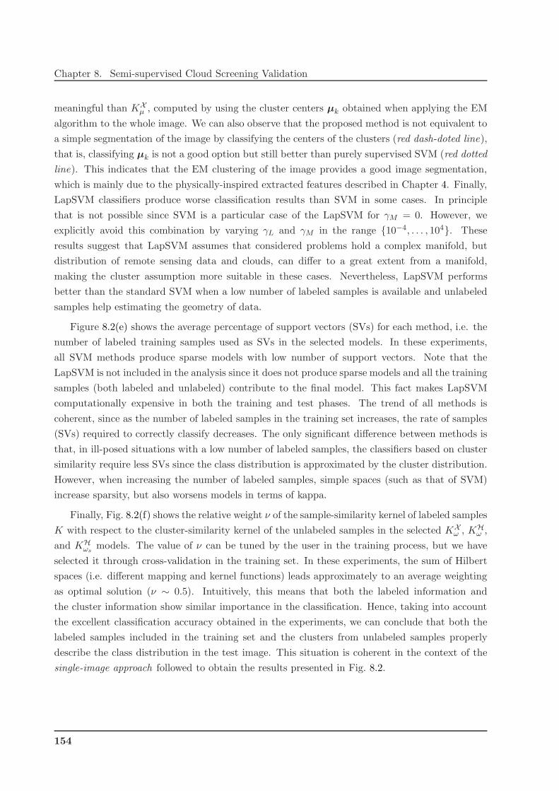
Chapter 8. Semi-supervised Cloud Screening Validation
meaningful than KXµ , computed by using the cluster centers µk obtained when applying the EM
algorithm to the whole image. We can also observe that the proposed method is not equivalent to
a simple segmentation of the image by classifying the centers of the clusters (red dash-doted line),
that is, classifying µk is not a good option but still better than purely supervised SVM (red dotted
line). This indicates that the EM clustering of the image provides a good image segmentation,
which is mainly due to the physically-inspired extracted features described in Chapter 4. Finally,
LapSVM classifiers produce worse classification results than SVM in some cases. In principle
that is not possible since SVM is a particular case of the LapSVM for γM = 0. However, we
explicitly avoid this combination by varying γL and γM in the range {10−4, . . . , 104}. These
results suggest that LapSVM assumes that considered problems hold a complex manifold, but
distribution of remote sensing data and clouds, can differ to a great extent from a manifold,
making the cluster assumption more suitable in these cases. Nevertheless, LapSVM performs
better than the standard SVM when a low number of labeled samples is available and unlabeled
samples help estimating the geometry of data.
Figure 8.2(e) shows the average percentage of support vectors (SVs) for each method, i.e. the
number of labeled training samples used as SVs in the selected models. In these experiments,
all SVM methods produce sparse models with low number of support vectors. Note that the
LapSVM is not included in the analysis since it does not produce sparse models and all the training
samples (both labeled and unlabeled) contribute to the final model. This fact makes LapSVM
computationally expensive in both the training and test phases. The trend of all methods is
coherent, since as the number of labeled samples in the training set increases, the rate of samples
(SVs) required to correctly classify decreases. The only significant difference between methods is
that, in ill-posed situations with a low number of labeled samples, the classifiers based on cluster
similarity require less SVs since the class distribution is approximated by the cluster distribution.
However, when increasing the number of labeled samples, simple spaces (such as that of SVM)
increase sparsity, but also worsens models in terms of kappa.
Finally, Fig. 8.2(f) shows the relative weight ν of the sample-similarity kernel of labeled samples
K with respect to the cluster-similarity kernel of the unlabeled samples in the selected KXω , KH
ω ,
and KHωs
models. The value of ν can be tuned by the user in the training process, but we have
selected it through cross-validation in the training set. In these experiments, the sum of Hilbert
spaces (i.e. different mapping and kernel functions) leads approximately to an average weighting
as optimal solution (ν ∼ 0.5). Intuitively, this means that both the labeled information and
the cluster information show similar importance in the classification. Hence, taking into account
the excellent classification accuracy obtained in the experiments, we can conclude that both the
labeled samples included in the training set and the clusters from unlabeled samples properly
describe the class distribution in the test image. This situation is coherent in the context of the
single-image approach followed to obtain the results presented in Fig. 8.2.
154

8.3. Semi-supervised Cloud Screening Validation Results
8.3.2 Image-Fold Approach Results
Now, we analyze the classification results when following the image-fold approach, i.e. each
test image is classified according to a model built with labeled samples from the other 4 images
and unlabeled samples coming from the same test image. This procedure is aimed at testing the
robustness of the algorithm to differences between the training and test distributions.
Figure 8.3(a) shows the κ statistic for the five images obtained with the standard SVM. This
plot provides us a reference of how difficult is the classification problem in each MERIS image,
but now it also depends on how well are the labeled samples from the other images in the training
set representing the classes in the test image. Now, the order of the images depending on its clas-
sification complexity is very similar: Barrax (BR-2003-07-14), Barrax (BR-2004-07-14), Tunisia
(TU-2004-07-15), France (FR-2005-03-19), and Finland (FI-2005-02-26). Also poorer classifica-
tion accuracy is obtained in all images as expected. However, it remains almost independent of
the number of labeled samples, which indicates that, from the very beginning, labeled samples
from other images roughly describe the type of clouds in the test image, and these situations do
not improve by adding more labeled samples with the same information. Therefore, we can con-
clude that, following the proposed image-fold approach, the experiments for the five images are
affected by sample selection bias problem. In the remaining plots of Fig. 8.3, the results obtained
for these five scenes are averaged in order to discover which method performs better in most of
the scenarios.
Figure 8.3(b) shows the average CPU time consumed by each method during the training
phase. The results in this plot are almost identical to the results in Fig. 8.2, since the computa-
tional burden mainly depend on the amount and type of data, and the experiments were carried
out in the same computer.
Figures 8.3(c) and 8.3(d) show the average κ and OA for all the methods. The situation now
is completely different to the previous experiments following the single-image approach. Almost
all the methods provide moderate classification results, and all of them provide poor results in ill-
posed situations. However, a great difference can be observed between the µ-SVM classifiers based
on clusters exclusively (‘◦’ markers) and the rest. Several conclusions can be obtained from these
curves. The standard SVM is affected by the sample selection bias and this can not be solved since
it relies on the training labeled samples exclusively. When using the standard SVM to directly
classify the centers of the clusters from the EM algorithm, classification results improve since, if
the training and the test data are different, it is difficult to learn from training samples and then
unsupervised approaches can be useful. Again, the main impediment is the SVM classifier used
to label the cluster centers. The LapSVM provides moderate classification results, but generates
better classification accuracy than the SVM in all cases since it incorporates in the solution the
geometry of the unlabeled samples that come from the test image. The µ-SVM classifiers based
exclusively on cluster-based approaches KXµ , KH
µ , and KHµs
provide excellent results when there
are enough labeled samples to describe the class conditional distribution of the clusters (with
155

Chapter 8. Semi-supervised Cloud Screening Validation
8 15 29 56 107 207 400−0.1
0
0.1
0.2
0.3
0.4
0.5
0.6
0.7
0.8
# Labeled Samples
Standard SVM Kappa statistic,κ
BARRAX (BR-2003-07-14)
BARRAX (BR-2004-07-14)
TUNISIA (TU-2004-07-15)
FINLAND (FI-2005-02-26)
FRANCE (FR-2005-03-19)
(a)
8 15 29 56 107 207 40010
−2
10−1
100
101
102
103
104
CP
U ti
me
[s]
# Labeled Samples
(b)
8 15 29 56 107 207 4000.45
0.5
0.55
0.6
0.65
0.7
0.75
Kap
pa s
tatis
tic,κ
# Labeled Samples
(c)
8 15 29 56 107 207 40072
74
76
78
80
82
84
86
88
Ove
rall
Acc
urac
y, O
A[%
]
# Labeled Samples
(d)
8 15 29 56 107 207 4000
20
40
60
80
100
SV
s [%
]
# Labeled Samples
(e)
8 15 29 56 107 207 4000.4
0.45
0.5
0.55
0.6
0.65
0.7
0.75
0.8
Wei
ght o
f sam
ple−
sim
ilarit
y ke
rnel
# Labeled Samples
(f)
Figure 8.3: Average cloud classification results for the 5 MERIS sample images training the models with
labeled samples from the other 4 images and 800 unlabeled samples from the image to be classified (image-
fold approach): κ of the standard SVM for each image, CPU time [s], avg(κ), avg(OA), SVs[%], and weight
ν of the sample-similarity kernel of labeled samples K. Symbols correspond to the legend in Table 8.2.
156

8.3. Semi-supervised Cloud Screening Validation Results
few labeled samples a whole cluster can be misclassified). Among these three classifiers, KHµ
produce worse results. This can be explained since the selection of the mapping function to H,
i.e. the selection of kernel free parameters, depends on the classification accuracy in the training
set. Therefore, an inappropriate training set produces an inappropriate mapping (in terms of
class separability in test). As a consequence, KHµ is more affected by the sample selection bias
since all the unlabeled samples in the training set are used to compute the cluster similarity in
an inappropriate kernel space. On the other hand, KXµ is more robust to the sample selection
bias because it approximates the cluster similarity to the similarities of the cluster centers µk
already defined in the input space, and thus it is less dependent on how the unlabeled samples
that represent the clusters are mapped into H. In this context, KHµs
provides the best results and
is also more robust to the sample selection bias because it uses the soft mean map to compute
the cluster similarity in the kernel space. The soft mean map weights the contribution of each
sample to the definition of the centre of mass of each cluster in the kernel space H with the EM
estimated posterior probabilities. This is equivalent to eliminate the samples that do not properly
represent the cluster in the input space, and thus the estimation of the cluster center in H is less
influenced by the selection of an inappropriate mapping. Finally, the µ-SVM classifiers based on
composite mean kernels KXω , KH
ω , and KHωs
(black ‘+’ lines) produce significant worse results than
the cluster-based approaches Kµ. These approaches combine both sample and cluster similarities
and, intuitively, should produce better classification results than standard SVM (K) and Kµ,
which are a particular case of Kω for ν = 1 and ν = 0, respectively. Therefore, the divergence in
the results should be explained because the tuning of ν, and we have to analyze also the selected
ν value for the different experiments.
Fig. 8.3(f) shows the relative weight ν of the sample-similarity kernel of labeled samplesK with
respect to the cluster-similarity kernel Kµ. In this plot, we can observe that for a low number
of labeled samples (ℓ 6 30) the sample-similarity and cluster-similarity has the same weight
(ν = 0.5), and then the weight of the sample-similarity kernel of labeled samples K increases
exponentially with the number of labeled samples. As the number of labeled samples increases,
K becomes more important than the cluster information (the exponential value of labeled samples
in supervised classifiers is analyzed in detail by Castelli and Cover (1995)). However, the opposite
behavior is observed in the classification accuracy (Fig. 8.3(c) and 8.3(d)) that starts to decreases
when ν increases. As mentioned above, the labeled samples in the training set used to compute
K come from different images and are affected by the sample selection bias. For this reason, high
values of ν (more weight of K) produce worse values. The key point is why high values of ν are
selected during the training. The reason is that ν has been selected through v-fold cross-validation
in the labeled training samples, thus the selected model (ν, σ, and C) will be biased towards the
training samples, which produces worse results in test if the training and test distributions are
significantly different. It should be noted that the model selection in semi-supervised methods
applied to problems affected by sample selection bias is not well-solved yet. A solution would be
to select the best model by cross-validation in a labeled validation set coming from the image to
157
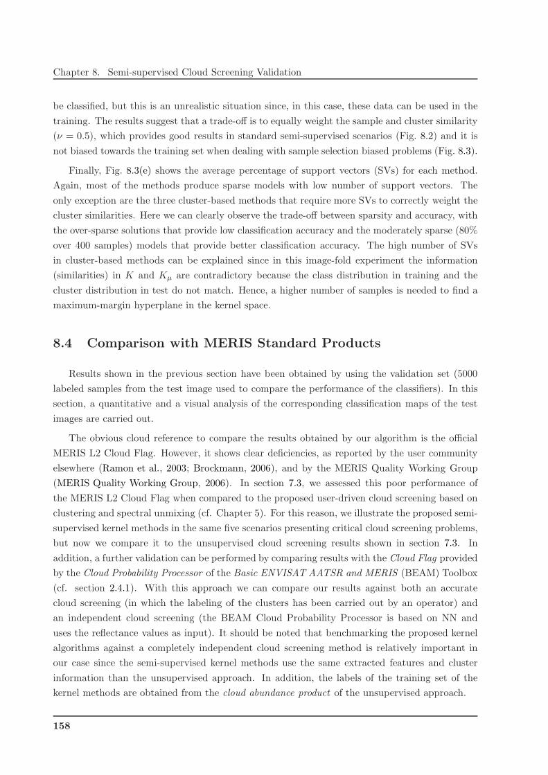
Chapter 8. Semi-supervised Cloud Screening Validation
be classified, but this is an unrealistic situation since, in this case, these data can be used in the
training. The results suggest that a trade-off is to equally weight the sample and cluster similarity
(ν = 0.5), which provides good results in standard semi-supervised scenarios (Fig. 8.2) and it is
not biased towards the training set when dealing with sample selection biased problems (Fig. 8.3).
Finally, Fig. 8.3(e) shows the average percentage of support vectors (SVs) for each method.
Again, most of the methods produce sparse models with low number of support vectors. The
only exception are the three cluster-based methods that require more SVs to correctly weight the
cluster similarities. Here we can clearly observe the trade-off between sparsity and accuracy, with
the over-sparse solutions that provide low classification accuracy and the moderately sparse (80%
over 400 samples) models that provide better classification accuracy. The high number of SVs
in cluster-based methods can be explained since in this image-fold experiment the information
(similarities) in K and Kµ are contradictory because the class distribution in training and the
cluster distribution in test do not match. Hence, a higher number of samples is needed to find a
maximum-margin hyperplane in the kernel space.
8.4 Comparison with MERIS Standard Products
Results shown in the previous section have been obtained by using the validation set (5000
labeled samples from the test image used to compare the performance of the classifiers). In this
section, a quantitative and a visual analysis of the corresponding classification maps of the test
images are carried out.
The obvious cloud reference to compare the results obtained by our algorithm is the official
MERIS L2 Cloud Flag. However, it shows clear deficiencies, as reported by the user community
elsewhere (Ramon et al., 2003; Brockmann, 2006), and by the MERIS Quality Working Group
(MERIS Quality Working Group, 2006). In section 7.3, we assessed this poor performance of
the MERIS L2 Cloud Flag when compared to the proposed user-driven cloud screening based on
clustering and spectral unmixing (cf. Chapter 5). For this reason, we illustrate the proposed semi-
supervised kernel methods in the same five scenarios presenting critical cloud screening problems,
but now we compare it to the unsupervised cloud screening results shown in section 7.3. In
addition, a further validation can be performed by comparing results with the Cloud Flag provided
by the Cloud Probability Processor of the Basic ENVISAT AATSR and MERIS (BEAM) Toolbox
(cf. section 2.4.1). With this approach we can compare our results against both an accurate
cloud screening (in which the labeling of the clusters has been carried out by an operator) and
an independent cloud screening (the BEAM Cloud Probability Processor is based on NN and
uses the reflectance values as input). It should be noted that benchmarking the proposed kernel
algorithms against a completely independent cloud screening method is relatively important in
our case since the semi-supervised kernel methods use the same extracted features and cluster
information than the unsupervised approach. In addition, the labels of the training set of the
kernel methods are obtained from the cloud abundance product of the unsupervised approach.
158
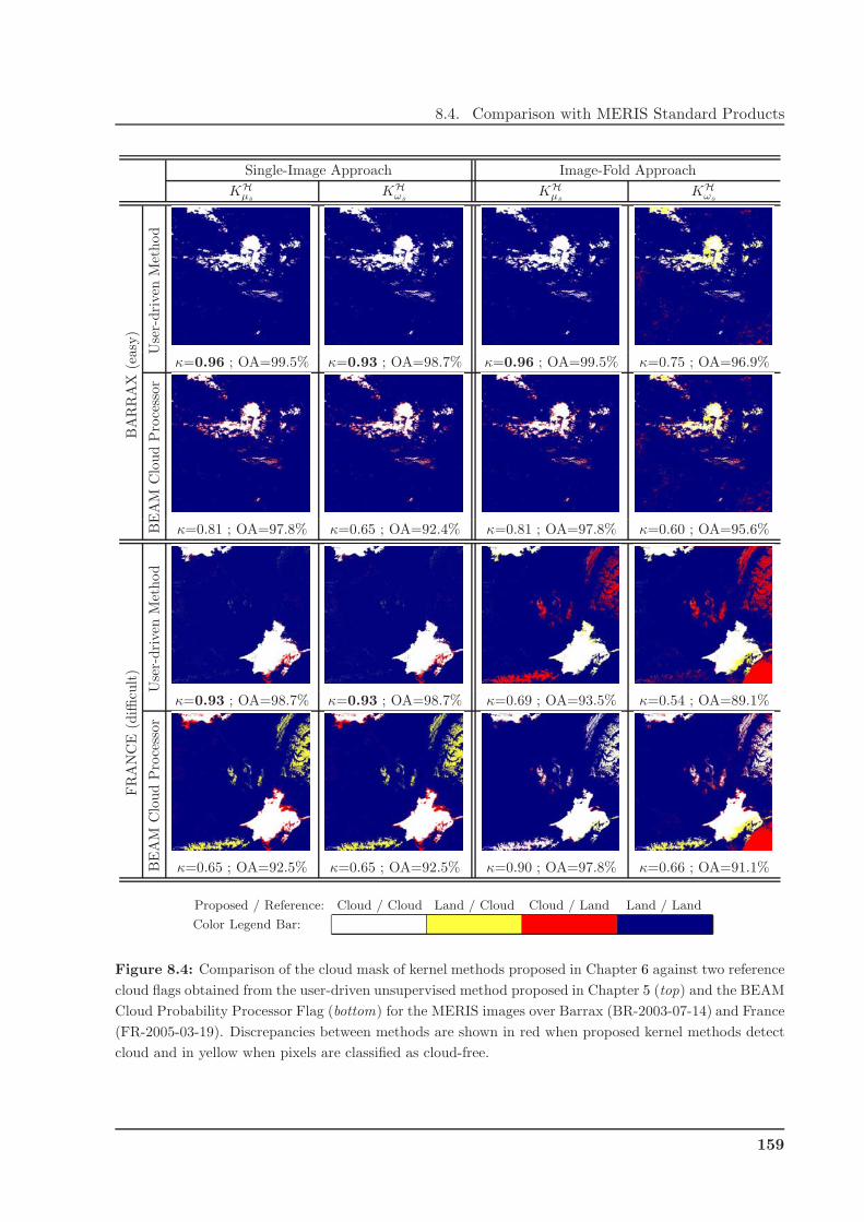
8.4. Comparison with MERIS Standard Products
Single-Image Approach Image-Fold Approach
KHµs
KHωs
KHµs
KHωs
BA
RR
AX
(easy
)
Use
r-dri
ven
Met
hod
κ=0.96 ; OA=99.5% κ=0.93 ; OA=98.7% κ=0.96 ; OA=99.5% κ=0.75 ; OA=96.9%
BE
AM
Clo
ud
Pro
cess
or
κ=0.81 ; OA=97.8% κ=0.65 ; OA=92.4% κ=0.81 ; OA=97.8% κ=0.60 ; OA=95.6%
FR
AN
CE
(diffi
cult)
Use
r-dri
ven
Met
hod
κ=0.93 ; OA=98.7% κ=0.93 ; OA=98.7% κ=0.69 ; OA=93.5% κ=0.54 ; OA=89.1%
BE
AM
Clo
ud
Pro
cess
or
κ=0.65 ; OA=92.5% κ=0.65 ; OA=92.5% κ=0.90 ; OA=97.8% κ=0.66 ; OA=91.1%
Proposed / Reference: Cloud / Cloud Land / Cloud Cloud / Land Land / Land
Color Legend Bar:
Figure 8.4: Comparison of the cloud mask of kernel methods proposed in Chapter 6 against two reference
cloud flags obtained from the user-driven unsupervised method proposed in Chapter 5 (top) and the BEAM
Cloud Probability Processor Flag (bottom) for the MERIS images over Barrax (BR-2003-07-14) and France
(FR-2005-03-19). Discrepancies between methods are shown in red when proposed kernel methods detect
cloud and in yellow when pixels are classified as cloud-free.
159

Chapter 8. Semi-supervised Cloud Screening Validation
Figure 8.4 shows the comparison of the µs-SVM methods (both composite KHωs
and cluster-
based KHµs
classifiers) against the cloud masks from the two cloud screening references. The cloud
flag of the user-driven method is computed by applying a threshold of 0.05 to the cloud abundance
product (cf. section 5.3.3), which in fact are the true labels for the trained models; and the flag of
the BEAM Cloud Processor indicates cloudy when the NN output is higher than 20%, which is the
lowest threshold recommended by the authors of the algorithm (Preusker et al., 2006). The images
selected to illustrate the results are one image over Barrax (BR-2003-07-14) and the France image
(FR-2005-03-19), which present different cloud screening problems and are differently affected
by the sample selection bias problem. In the case of the unprojected MERIS FR images, the
quarter scenes have 1153×1153 pixels (e.g. BR-2003-07-14) and the full scenes have 2241×2241
pixels (e.g. FR-2005-03-19). The selected images are classified using the best models (realization
with best validation results) trained with 400 labeled samples for both the single-image approach
and the image-fold approach (last point in the figures 8.2 and 8.3, respectively). Pixels where
compared algorithms agree are depicted in white for the cloudy pixels and in blue for the cloud
free pixels; discrepancies are shown in yellow and red. The agreement between both methods is
expressed in terms of the overall accuracy (OA) and kappa statistic (κ) for the whole image.
Classification accuracies higher than 90% are obtained for most cases, but the lower values of
κ for some cases reflect that classification results are unbalanced due to the misclassification of a
significant number pixels of one class. Note that the overall accuracy is directly interpretable as
the ratio of pixels being classified correctly, while the kappa coefficient allows for a statistical test
of the significance of the divergence between two algorithms (Congalton and Green, 1999). The
best kappa result (>0.9) for each experiment is bold faced. First, we are going to analyze the
classification on the Barrax image, which represents an easy cloud screening problem. Looking at
the comparisons with both the ‘User-driven Method’ and the ‘BEAM Cloud Processor’ references,
one can observe that the kernel methods and the user-driven unsupervised method show a good
agreement, while the BEAM product misclassifies the cloud borders (red pixels) where only our
algorithms detect cloudy pixels. When comparing the two kernel methods with the user-driven
reference, the cluster-based classifier KHµs
provides good results even in the image-fold approach,
which means that training samples from the other images are useful to correctly classify the
clusters found in the test image. However, the composite kernel classifier KHωs
works properly in
the single-image approach, while results are worse for the image-fold approach, which means that
the model is biassed towards the labeled samples of the other images instead of to the cluster
structure (see explanation of Fig. 8.3(f)).
The second image is the ‘France image’, which presents opaque clouds at south and north
and also snow in the Alps, the Pyrenees, and the Massif Central. Attending to the image-fold
experiments, µs-SVM methods agree with the user-driven cloud mask, and the discrepancies
with the BEAM Processor show evidence of the errors committed by the BEAM Processor that
misclassifies all the snowy areas as clouds. In the image-fold approach, neither the cluster-based
classifierKHµs
nor the composite kernel classifierKHωs
produce an accurate cloud screening. This can
160

8.4. Comparison with MERIS Standard Products
Brightness (fBr,VIS) Oxygen (fO2) Water Vapor (fWV)
BA
RR
AX
(easy
)
0 0.2 0.4 0.6 0.8 10
0.02
0.04
0.06
0.08
0.1
0.1 0.2 0.3 0.4 0.5 0.6 0.7 0.80
0.02
0.04
0.06
0.08
0.1
0.12
0.14
0.16
0.18
0 0.2 0.4 0.6 0.8 10
0.02
0.04
0.06
0.08
0.1
0.12
FR
AN
CE
(diffi
cult)
0 0.2 0.4 0.6 0.8 10
0.05
0.1
0.15
0.2
0.25
0.1 0.2 0.3 0.4 0.5 0.6 0.7 0.80
0.02
0.04
0.06
0.08
0.1
0.12
0.14
0 0.2 0.4 0.6 0.8 10
0.02
0.04
0.06
0.08
0.1
0.12
0.14
Surface (Train)Cloudy (Train)Surface (Test)Cloudy (Test)
Figure 8.5: Comparison of the class conditional distributions of the brightness (fBr,VIS, right), oxygen
(fO2, center), and water vapor (fWV, left) features for the MERIS images over Barrax (BR-2003-07-14, top)
and France (FR-2005-03-19, bottom). The class conditional distributions are obtained from the normalized
histograms of each class; and, in the case of the training distributions (red curves), the histograms of each
experiment were obtained with all the pixels from the other four images (image-fold approach).
be explained since, in the image-fold approach, no training samples from the other images model
the difference between clouds and snowy mountains, thus the classifier can not learn this difference
(as probably happens with the NN trained for BEAM). Therefore, although the proposed semi-
supervised methods benefit from the inclusion of unlabeled samples by estimating the marginal
data distribution, these methods are limited by the quality of the available labeled information
and can not alleviate situations with a dramatic sample selection bias problem.
Figure 8.5 illustrates the origin of the sample selection bias caused when the training set
is formed by samples coming from images different to the image to be classified (image-fold
approach). In this figure, the class conditional distributions (pdf) of some extracted features for
the training images and test image are displayed. Two main conclusions can be extracted from
these plots. On the one hand, the distributions of the two classes (solid-line for ‘Surface’ and
dashed line for ‘Cloudy’) in the test image (black color) are more overlapped for all the extracted
features from the France image, which confirms the higher difficulty to classify the France image
than the Barrax image. On the other hand, the ‘Surface’ and ‘Cloudy’ distributions on training
(image-fold approach, red) are much more different than the ‘Surface’ and ‘Cloudy’ distributions
on test (black), respectively, for the case of France image classification. Summarizing, the France
image is intrinsically more difficult to classify due to the class overlap, and it is more affected
161
Chapter 8. Semi-supervised Cloud Screening Validation
by the sample selection bias due to the lack of representativeness of the test class conditional
distribution in the training images.
8.5 Results on MERIS Temporal Series
Let us start by formally reviewing the main differences between the single-image approach and
the image-fold approach in a multitemporal classification context. In multitemporal classification,
one tries to classify the pixels of an image at the observation time tN by using the available
(instantaneous or previous) information t 6 tN . In these experiments, we follow a cascade strategy
for classification, i.e. only the previous acquired information is used to classify a given image. This
strategy differs from a strategy in which the posterior images are also used. Therefore, under the
semi-supervised learning framework, two main situations may arise, depending on the availability
of information at the classification time t = tN .
1. Labeled information is available only for t < tN . This is the most common scenario and
discourages the use of fully supervised classifiers, such as the SVM, that learn to discriminate
classes at t < tN and then are used to extrapolate their predictions at t = tN . This scenario
is simulated in the experiments by a multitemporal image-fold approach where models are
trained using both labeled samples from t1 to tN−1 images, and unlabeled samples from the
image to be classified tN .
2. Labeled information is available for t = tN . This single-image situation makes the use of
supervised classifiers, such as SVM, more appropriate, but unlabeled data still can help in
the classification when a reduced number of labeled data is available.
For the experiments, the temporal series of MERIS FR Level 1b images acquired over The
Netherlands in 2003 are used to illustrate our approach. Most of the images are the same as in
Fig. 7.5, but different dates/images are chosen since the criterion now is to select images with
both cloudy and cloud-free areas. In addition, now we are not restricting ourselves to use one
image per month in order to capture the phenological cycle of land covers. In fact, close dates
are better suited for an image-fold approach since land covers should not change. Therefore,
an uneven temporal series of 12 images is considered in the multitemporal image-fold approach:
February 18th, April 22nd, April 23rd, May 28th, May 31st, June 6th, June 16th, August 6th,
August 8th, August 9th, and August 12th. In addition, no co-registration or even projection
of the images is required, since now we are not interested in land properties and the proposed
multitemporal approach requires samples from different dates but not all the dates for a given
location. In this context, the models are trained using both labeled samples from the tN−2 and
tN−1 available images, and unlabeled samples from the image to be classified tN , i.e. 2-image-fold
approach where only the two closest previous images are used. Note that, following this approach,
only ten images will be classified since the images of 18th February and 22nd April are only used
162

8.5. Results on MERIS Temporal Series
8 15 29 56 107 207 4000.55
0.6
0.65
0.7
0.75
0.8
0.85
0.9
0.95
1
# Labeled Samples
Sta
nd
ard
SV
M K
ap
pa
sta
tistic,κ
Netherlands (2003-04-23)Netherlands (2003-05-28)Netherlands (2003-05-31)Netherlands (2003-06-06)Netherlands (2003-06-16)Netherlands (2003-07-08)Netherlands (2003-08-06)Netherlands (2003-08-08)Netherlands (2003-08-09)Netherlands (2003-08-12)
(a)
8 15 29 56 107 207 40010
−2
10−1
100
101
102
103
104
CP
U ti
me
[s]
# Labeled Samples
(b)
8 15 29 56 107 207 4000.7
0.75
0.8
0.85
0.9
0.95
1
Kap
pa s
tatis
tic,κ
# Labeled Samples
(c)
8 15 29 56 107 207 40085
90
95
100O
vera
ll A
ccur
acy,
OA
[%]
# Labeled Samples
(d)
8 15 29 56 107 207 4000
20
40
60
80
100
SV
s [%
]
# Labeled Samples
(e)
8 15 29 56 107 207 4000.4
0.45
0.5
0.55
0.6
0.65
0.7
0.75
0.8
Wei
ght o
f sam
ple−
sim
ilarit
y ke
rnel
# Labeled Samples
(f)
Figure 8.6: Average cloud classification results for 10 MERIS images over The Netherlands training the
models with labeled and unlabeled (800) samples from the image to be classified (single-image approach):
κ of the standard SVM for each image, CPU time [s], avg(κ), avg(OA), SVs[%], and weight ν of the
sample-similarity kernel of labeled samples K. Symbols correspond to the legend in Table 8.2.
163

Chapter 8. Semi-supervised Cloud Screening Validation
to generate the training set of 23rd April and half of the training set of 28th May. For additional
details about the experimental setup see section 8.1 and for the used kernel methods and the
model development see section 8.2.
The same procedure that in section 8.3 is followed in order to analyze the performance of the
classifiers on the temporal series of MERIS images acquired over The Netherlands. Average results
over ten realizations for different rates of labeled samples are shown in Fig. 8.6 and Fig. 8.7 for
the single-image and the image-fold approach, respectively. Several conclusions can be obtained
from these plots.
Figure 8.6(a) shows the κ statistic for the ten images obtained with the standard SVM, which
indicates that the classification complexity of the images is almost the same except for ill-posed
situations where semi-supervised methods should provide better results. In the remaining plots
of Fig. 8.6, the results obtained for the ten dates are averaged in order to discover which method
performs better in most situations. The discussion about the CPU time consumed by each method
in Fig. 8.6(b) has already been done for Fig. 8.2. The average κ and OA for all the methods are
shown in Fig. 8.6(c) and 8.6(d), respectively. The main conclusion extracted from the curves is
that the proposed µ-SVM method clearly improves the results of the other methods, especially
when the cluster similarity is computed in the kernel space H by using the mean map. In fact, the
µ-SVM classifiers follow a similar trend that the purely supervised SVM (red dotted line), which
means that the labeled information is crucial to obtain accurate results, but the cluster structure
of the test image properly adapts the classification mapping if the EM produces a good image
segmentation. In the case of the LapSVM, different behaviors can be observed depending on
the labeled samples. Only when a low number of labeled samples is available LapSVM performs
better than the standard SVM thanks to the unlabeled samples that help estimating the geometry
of data distribution. Finally, the percentage of SVs for all the methods (Fig. 8.6(e)) is almost
the same since, in the single image approach, the class distribution is well-defined by the labeled
samples in the training set and the same key samples are used in all the methods to define the
class boundary. The gain in accuracy of the semi-supervised µ-SVM classifiers is not obtained
by adding more labeled samples to the final model but taking also into account the similarities
between the clusters of the selected SVs. This can be observed in Fig. 8.6(f) that shows how the
sample-similarity K and cluster-similarity Kµ equally contribute in the best models (ν ∼ 0.5).
Figure 8.7 shows the classification results for the same images when following the multitem-
poral image-fold approach. The κ statistic for the ten images obtained with the standard SVM
(Fig. 8.7(a)) evidences the decrease in the classification accuracy, which is also much more variable,
due to the sample selection bias (i.e., in some cases, the labeled samples from the two previous
images do not represent the classes in the test image). However, the worsening of the results now
is lower than for the images of section 8.3 since the problems in contiguous images of the temporal
series are similar (land covers, location, etc.). The CPU times in Fig. 8.7(b) are almost identical
to the results in Fig. 8.2, since the computational burden mainly depends on the amount and
type of data, and the labeled samples are the same and experiments were carried out in the same
164

8.5. Results on MERIS Temporal Series
8 15 29 56 107 207 4000.2
0.3
0.4
0.5
0.6
0.7
0.8
0.9
1
# Labeled Samples
Sta
nd
ard
SV
M K
ap
pa
sta
tistic,κ
Netherlands (2003-04-23)Netherlands (2003-05-28)Netherlands (2003-05-31)Netherlands (2003-06-06)Netherlands (2003-06-16)Netherlands (2003-07-08)Netherlands (2003-08-06)Netherlands (2003-08-08)Netherlands (2003-08-09)Netherlands (2003-08-12)
(a)
8 15 29 56 107 207 40010
−2
10−1
100
101
102
103
104
CP
U ti
me
[s]
# Labeled Samples
(b)
8 15 29 56 107 207 4000.5
0.55
0.6
0.65
0.7
0.75
0.8
0.85
0.9
Kap
pa s
tatis
tic,κ
# Labeled Samples
(c)
8 15 29 56 107 207 40076
78
80
82
84
86
88
90
92
94O
vera
ll A
ccur
acy,
OA
[%]
# Labeled Samples
(d)
8 15 29 56 107 207 4000
20
40
60
80
100
SV
s [%
]
# Labeled Samples
(e)
8 15 29 56 107 207 4000.4
0.45
0.5
0.55
0.6
0.65
0.7
0.75
0.8
Wei
ght o
f sam
ple−
sim
ilarit
y ke
rnel
# Labeled Samples
(f)
Figure 8.7: Average cloud classification results for 10 MERIS images over The Netherlands training the
models with labeled samples from the two previous images over The Netherlands and 800 unlabeled samples
from the image to be classified (temporal image-fold approach): κ of the standard SVM for each image,
CPU time [s], avg(κ), avg(OA), SVs[%], and weight ν of the sample-similarity kernel of labeled samples
K. Symbols correspond to the legend in Table 8.2.
165

Chapter 8. Semi-supervised Cloud Screening Validation
computer. Figures 8.7(c) and 8.7(d) show the average κ and OA for all the methods. Again, the
situation is less dramatic than in the previous experiments of section 8.3 since the images of the
temporal series are less affected by the sample selection bias problem. For this reason, although
the mean classification accuracy is lower, the differences among methods are similar to those of
the single-image approach in Fig. 8.6. Only for the µ-SVM cluster-based classifier KXµ a signifi-
cant lower classification accuracy is observed, which suggests that, for the image-fold approach,
the centers of the clusters of previous images µt−ik can not properly model the clusters of the test
image and better results are obtained when computing the cluster similarity in the kernel space.
Regarding the average percentage of SVs in Fig. 8.7(e), the three cluster-based methods require
more SVs to correctly weight the cluster similarities. This result agrees with the curves found for
the previous image-fold experiments (Fig. 8.3), where the information (similitudes) in K and Kµ
are contradictory because the class distribution in training and the cluster distribution in test do
not match. Hence, a higher number of samples is needed to find the optimum classifier.
Finally, the relative weight ν of the sample-similarity kernel of labeled samples K with respect
to the cluster-similarity kernel Kµ (Fig. 8.7(f)) shows the expected behavior for the image-fold
experiments. Again, the weight of the sample-similarity kernel of labeled samples K increases
exponentially with the number of labeled samples (with more labeled samples K becomes more
important than the cluster information). Nevertheless, since in the temporal series of images
the sample selection bias problem is not so hard, ν increases slowly with the number of labeled
samples and the classification accuracy is less affected. Therefore, although the selected model
(ν) is biased towards the training samples, results in test are not so bad because the training and
test distributions are not so different.
Once the classification results over the validation set (5000 labeled samples from the test
image used to compare the performance of the classifiers) have been discussed, the classification
maps are generated for the ten test images. For the studied MERIS temporal series over The
Netherlands, only MERIS FR Level 1b products are available. Therefore, it is not possible to
compare the official L2 cloud flag with the cloud mask produced by the kernel methods. The
cloud mask provided by the BEAM Cloud Probability Processor is available but, as we have
shown in sections 7.4.2 and 8.4, this algorithm fails in some critical cloud screening problems.
In consequence, we restrict ourselves to compare the classification maps of the composite mean
kernel classifier (KHωs
) with the user-driven cloud screening method that provides the most accurate
ground truth (computed by applying a threshold of 0.05 to the cloud abundance product). The
images are classified using the best model (realization with best validation results) trained with
400 labeled samples for the single-image approach (last point in Fig.8.6).
Figure. 8.8 shows the RGB color images for the temporal series of MERIS images with cloud
covers over The Netherlands in 2003 together with the cloud mask provided by the proposed kernel
method based on composite and mean kernels, KHωs
. Note that the images are not projected in any
geo-reference system and thus the image size of all the MERIS FR scenes is 2241 × 2241 and the
166
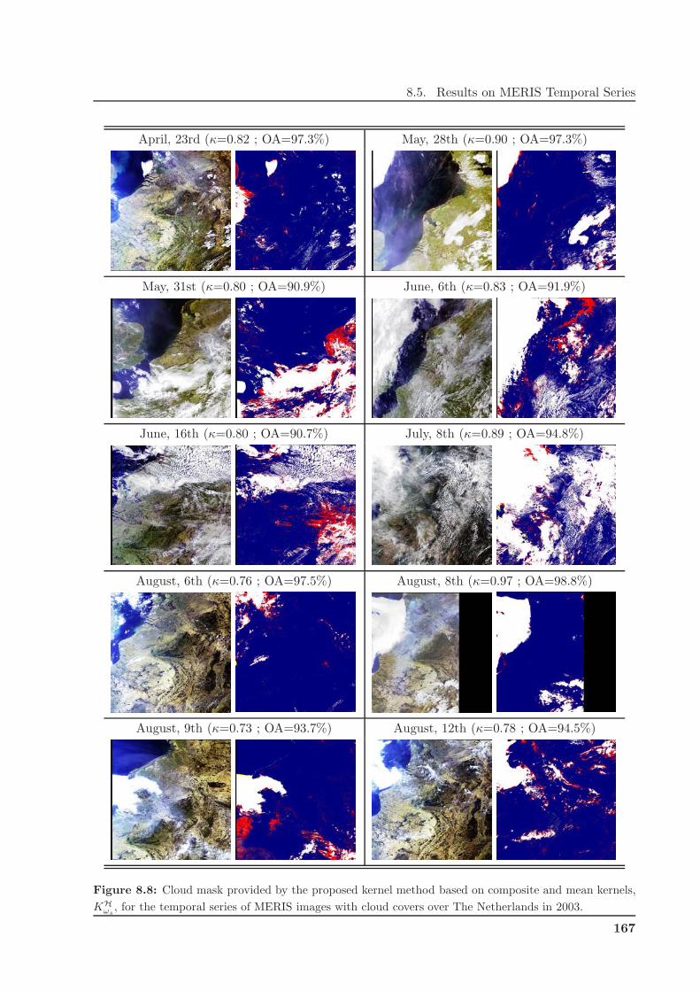
8.5. Results on MERIS Temporal Series
April, 23rd (κ=0.82 ; OA=97.3%) May, 28th (κ=0.90 ; OA=97.3%)
May, 31st (κ=0.80 ; OA=90.9%) June, 6th (κ=0.83 ; OA=91.9%)
June, 16th (κ=0.80 ; OA=90.7%) July, 8th (κ=0.89 ; OA=94.8%)
August, 6th (κ=0.76 ; OA=97.5%) August, 8th (κ=0.97 ; OA=98.8%)
August, 9th (κ=0.73 ; OA=93.7%) August, 12th (κ=0.78 ; OA=94.5%)
Figure 8.8: Cloud mask provided by the proposed kernel method based on composite and mean kernels,
KHωs
, for the temporal series of MERIS images with cloud covers over The Netherlands in 2003.
167
Chapter 8. Semi-supervised Cloud Screening Validation
area displayed is not exactly the same. Pixels where compared algorithms agree are depicted in
white for the cloudy pixels and in blue for the cloud free pixels; discrepancies are shown in yellow
and red. The agreement between both methods is expressed in terms of the overall accuracy
(OA) and estimated kappa statistic (κ) for the whole image. In the figure, we can appreciate the
excellent classification accuracies higher than 90% obtained for all cases. Also κ shows balanced
classification results higher than 0.7 even in the worst cases. In addition, one can observe that
the kernel methods and the user-driven unsupervised method show an excellent agreement, and
most of the discrepancies correspond to the cloud borders (red pixels) where it is really difficult
to distinguish the level of cloud contamination in the measured pixel.
8.6 On the Relative Importance of Labeled and Unlabeled Sam-
ples
In the previous sections, performance of the supervised and semi-supervised kernel methods in
different situations has been analyzed. In the experiments, we have explored the robustness of the
classifiers to the number of labeled samples available during the training process; from ill-posed
situations with only 4 labeled samples per class (ℓ = 8) up to well-posed supervised cases with 200
labeled samples per class (ℓ = 400). In addition, for the semi-supervised methods, the number of
unlabeled samples (randomly selected from the analyzed test image) used in the training of the
models is fixed to u = 800. However, in the case of semi-supervised learning, it is also interesting
to analyze the capability of the different SSL methods to exploit the information contained in
the wealth of unlabeled samples. Therefore, additional experiments have been carried-out, in
which the number of both labeled and unlabeled samples is varied independently, in order to
see how efficiently the classifiers learn from the unlabeled samples, and how much the classifier
performance improves.
Fig. 8.9 shows the κ surface of the different methods as a function of the number of labeled (ℓ)
and unlabeled (u) samples used in the training phase. Note that the variation of u is two times
the variation of ℓ since unlabeled samples can be easily obtained from the test image. Moreover,
all experiments consider a minimum number of one hundred unlabeled samples since the cluster-
based methods require a proper representation of the clusters found in the test image in order to
provide reasonable classification results (though this is not a critical requirement). The κ surface is
shown for the standard SVM, the LapSVM, and the proposed µs-SVM classifiers KHωs
(0 < ν < 1)
and KHµs
(ν = 0). It is worth noting that the SVM is a fully supervised method and it is only
based on labeled samples. Therefore, the κ surface in Fig. 8.9(a) represents actually a single
curve since it is independent on the number of unlabeled samples. Results in Fig. 8.9 illustrate
only the image-fold approach since the value of unlabeled samples can be better evaluated when
labeled samples do not perfectly define the class distribution in the test image (sample selection
bias problem).
168

8.6. On the Relative Importance of Labeled and Unlabeled Samples
815
2956
107207
400
112
214
414
8000.4
0.5
0.6
0.7
# Labeled Samples# Unlabeled Samples
Kap
pa s
tatis
tic, κ
(a) SVM (Kℓ×ℓ)
815
2956
107207
400
112
214
414
8000.4
0.5
0.6
0.7
# Labeled Samples# Unlabeled Samples
Kap
pa s
tatis
tic, κ
(b) LapSVM (K(ℓ+u)×(ℓ+u))
815
2956
107207
400
112
214
414
8000.4
0.5
0.6
0.7
# Labeled Samples# Unlabeled Samples
Kap
pa s
tatis
tic, κ
(c) µs-SVM (KHωs
)
815
2956
107207
400
112
214
414
8000.4
0.5
0.6
0.7
# Labeled Samples# Unlabeled Samples
Kap
pa s
tatis
tic, κ
(d) µs-SVM (KHµs
)
Figure 8.9: Average cloud classification results for the 5 MERIS sample images (BR-2003-07-14, BR-
2004-07-14, TU-2004-07-15, FR-2005-03-19, and FI-2005-02-26) training the model for each image with
labeled samples from the other 4 images and unlabeled samples from the image to be classified (image-
fold approach): Kappa statistic surface over the validation set for the SVM, LapSVM, and µs-SVM as a
function of the number of labeled (ℓ) and unlabeled (u) samples.
The κ surface for the standard SVM (Fig. 8.9(a)) provides us with a baseline of κ and shows
its dependence on the number of labeled samples. This plot illustrates how the more supervised
information is available (high ℓ), the more accurate should be the classification for all methods.
However, due to the sample selection bias problem, when ℓ is high enough, the model is biased to-
wards the labeled training samples, which produces worse results in test since the training and test
distributions are significantly different. On Fig. 8.9(b), the κ surface for the LapSVM confirms, in
general terms, the importance of the labeled information in this problem. The LapSVM benefits
from the information of unlabeled samples, since it provides better results than the standard SVM
in all cases. However, classification accuracy slightly improves with the number of unlabeled sam-
ples, which suggests a preference for the regularization of the classifier (supervised information)
than for the regularization of the geometry of the marginal data distribution (unsupervised infor-
mation). Finally, the κ surfaces obtained for both µ-SVM methods are significantly different. The
KHωs
classifier (Fig. 8.9(c)) is affected by the sample selection bias problem for high values of ℓ as
the standard SVM. As explained in section 8.3.2, in the image-fold experiments, the KHωs
model is
169
Chapter 8. Semi-supervised Cloud Screening Validation
also biased towards the labeled training samples since ν is selected through v-fold cross-validation
in the labeled training samples. On the other hand, KHµs
(Fig. 8.9(d)) confirms the importance of
both labeled and unlabeled information in this problem. It uses both the labeled samples to fix
a support for the class distribution, and the unlabeled samples to characterize (parametrize) the
marginal distribution of data. The key point is that the proposed µ-SVM methods integrate the
test data distribution through the cluster distribution of the test image, which has been estimated
with the EM algorithm for GMM using the information contained in the high number of available
unlabeled pixels (or even all the image pixels) and not only with the unlabeled samples included
in the training set that the µ-SVM uses to determine cluster similarities.
The observed facts confirm the fact that semi-supervised learning methods require a much more
unlabeled samples than labeled for a noticeable gain in the classification accuracy, as suggested by
Castelli and Cover (1995, 1996) and Sinha and Belkin (2008). However, this implies an extremely
high computational cost in kernel methods. We have mitigated these problems by using the EM
algorithm as a preprocessing stage of the µ-SVM (note that the simplest and best understood
situation is when the data is described by an identifiable mixture model and each class comes
from a pure component). This approach falls in the field of cluster kernels, which are focused on
changing the representation given to a classifier by taking into account the structure described
by the unlabeled data (Szummer and Jaakkola, 2002; Zhu and Ghahramani, 2002; Chapelle et al.,
2003; Weston et al., 2005). We should note that even though the approach alleviates the problem,
there is still more room for improvement in the form of ‘learned’ kernels for specific datasets, or
by increasing the computational capabilities of kernel methods. We should stress here that novel,
fast, and linearly scalable SSL kernel methods are still required for remote sensing applications.
Recently, a great interest has been put on large scale kernel machines (Bottou et al., 2007).
170

Part IV
Conclusions


Chapter 9
Discussion and Conclusions
9.1 Summary and Conclusions
This Thesis presented a novel methodology in order to solve the challenging problem of cloud
screening in optical Earth Observation images acquired by multispectral and hyperspectral space-
borne sensors working in the visible and near-infrared range of the electromagnetic spectrum.
Sensors on board two European Space Agency environmental satellites are used in this work: the
MEdium Resolution Imaging Spectrometer (MERIS), placed on board the biggest environmen-
tal satellite ever launched (ENVISAT); and the Compact High Resolution Imaging Spectrometer
(CHRIS) hyperspectral instrument, mounted on board the technology demonstration mission
PROBA.
The proposed methodology identifies clouds in the image and produces a cloud abundance
map in order to quantify how cloud presence affects the measured spectra. The cloud screening
algorithm is based on well-founded physical features, which are intended to increase separability
between clouds and ground covers, and are extracted from the converted TOA reflectance in order
to reduce dependence on illumination and geometric acquisition conditions. A significant effort
has been done to correct and calibrate images from the selected sensors in order to ensure the
quality of data. In this respect, a novel algorithm has been proposed for the pre-processing of
push-broom hyperspectral sensors, which is especially relevant in the case of the CHRIS sensor.
The final objective has been to develope an accurate and automated set of tools for the
discrimination of clouds. For this purpose, two different approaches have been proposed depending
on whether the algorithm has to be applied on an operational basis to automatically classify
a significant number of images, or the classification process can be driven by an operator to
accurately identify even the most critical cloud screening problems. Both approaches use, as
the starting point, an unsupervised clustering method based on the extracted features in order
to adapt the cloud screening procedure to the situation of each image, mainly the atmospheric
conditions, the background, and the existing cloud types. This step allows to easily discriminate
Chapter 9. Discussion and Conclusions
between cloud-free and cloudy regions, providing a cloud abundance product based on a spectral
unmixing algorithm.
In the following paragraphs, several remarks and conclusions are drawn from the different
modules and algorithms developed in this Thesis.
Image Pre-processing. The first step of the process is to correct remote sensing data in
order to obtain an accurate TOA radiance signal. Note that correcting and compensating im-
age data from uncertainties in sensor calibration makes data to be independent from the sensor
system. This requires a deep understanding of the signals provided by ENVISAT/MERIS and
PROBA/CHRIS imaging spectrometers in order to adapt the cloud screening algorithm, or even
developing completely new correction algorithms.
• The smile effect produces small variations of the spectral wavelength of each pixel in the
across-track direction that have a large impact on the oxygen absorption feature, which is
extremely narrow. Therefore we have proposed a novel feature extraction algorithm that
allows the introduction of the spectral shift on the MERIS response in our formulation.
• PROBA is a technology demonstration satellite and several noise reduction algorithms have
been developed ad-hoc since CHRIS provides minimally preprocessed data.
• A new technique has been presented in order to detect pixels presenting drop-outs and
correct them by making use of both spatial and spectral information of the drop-out pixel
and its neighbors. Although it is a ‘cosmetic’ correction, it is needed since later processing
stages are drastically affected by these anomalous pixel values.
• A new technique has been presented to reduce the coherent noise known as vertical striping,
which is usually found in hyperspectral images acquired by push-broom sensors such as
CHRIS. The main novelty of our proposal consists in reducing the vertical striping pattern
using a new algorithm robust to surface changes.
• The proposed destriping approach has proven to be robust, stable, and permitted to success-
fully model the relationship of the sensor temperature with the magnitude and distribution
of the vertical striping.
Feature Extraction. When working with remote sensing images at different times and loca-
tions, a desirable characteristic is having data independent of the image acquisition conditions.
Converting TOA radiance data into TOA reflectance has the advantage that these data are
corrected for seasonal and diurnal differences in solar position. Moreover, extracting appropriate
physically-based features increases separability between clouds and ground covers, which improves
the classification performance and allows a better understanding of the problem.
174
9.1. Summary and Conclusions
We should note that, in addition to the brightness and whiteness radiometric properties of
clouds, one critical feature introduced in this work is the use of the atmospheric oxygen and water
vapor absorption bands to improve cloud screening results.
• The use of atmospheric absorption in the oxygen-A band to infer cloud pressure, which
is related to cloud-top height, is well-known in atmospheric studies. Here, we proposed a
formulation to extract an atmospheric feature directly related with the optical path by using
the exact pixel geometry.
• The oxygen absorption band is extremely narrow and, despite the high spectral and radio-
metric resolution of MERIS, small variations of the spectral wavelength of each pixel have
a large impact on any variable derived from the oxygen-A. As mentioned, this spectral shift
has been accounted for in order to correct the smile effect.
• In the case of CHRIS, the oxygen band is not so necessary because of CHRIS broader
bandwidths. However, some CHRIS acquisition modes present an excellent characterization
of the water vapor absorption.
• The maximum water vapor absorption (940 nm) is located outside the MERIS range but ab-
sorption at 900 nm is still valid for relative measurements inside the same image. Moreover,
snow presents higher absorption than clouds at 900 nm and this behavior can be observed
in the extracted feature.
• Results obtained by using these absorption features suggest that it would be advantageous
to see those bands included in future sensors.
• Specifically, the study has led to a qualitative list of key issues and physical features which
can potentially enhance cloud detection in remote sensing sensors working in the visible and
near-infrared spectrum: the target spectral brightness and whiteness in the VIS and the
NIR region, and the oxygen and water vapor atmospheric absorptions.
Cloud Screening. A central objective of the Thesis has been to provide new operational cloud
screening tools for the derivation of cloud location maps from the selected sensors’ data. In order
to achieve this objective, advanced pattern recognition and machine learning techniques have been
specifically developed.
• Two different cloud screening approaches have been proposed based on the assumption that
the available unlabeled samples in the remote sensing images have to be exploited.
• An unsupervised cloud screening approach based on classical pattern recognition methods
is proposed.
175

Chapter 9. Discussion and Conclusions
• Applying unsupervised clustering methods to the whole image allows us to take advantage
of the wealth of information and the high degree of spatial and spectral correlation of the
image pixels.
• The EM algorithm applied to the extracted features has shown an excellent ability to seg-
ment the image pixels allowing to easily discriminate between cloudy and cloud-free regions.
• A specific procedure has been defined to label the found clusters in order to assist an operator
to identify even the most critical cloud screening problems in regional and case studies.
• Advanced semi-supervised learning methods are explored since they offer the opportunity
of exploiting available labeled samples and the wealth of unlabeled samples. In this case,
some supervised information is available and is used together with the unlabeled samples
of the analyzed image to develop a classifier that provides the class of each pixel but taking
also into account the image data distribution. Since class distribution is partially fixed by
a training set, this method can be automatically applied to a large number of scenes in an
operational mode.
• A novel family of kernel methods based on the composite and mean kernels is proposed and
benchmarked to the standard SVM, which is used as a reference for supervised methods,
and the Laplacian SVM, which is used as a reference for semi-supervised methods.
• The proposed mean-map SVM (µ-SVM) combines both the sample similarity, computed
from the labeled samples in the training set, and the cluster similarity, computed from the
unlabeled samples of the test image in the kernel space through composite kernels.
• With this approach, the class distribution of typically low number of labeled samples is
adapted to the data distribution in the analyzed image estimated from the unlabeled samples.
As a consequence, the proposed approach is more robust to the sample selection bias, which
is a common statistical problem in real Earth Observation applications.
Cloud Abundance. One of the key requirements imposed to the proposed cloud screening
methodology was to provide information about the contribution of clouds to the spectra of image
pixels (for both transparent clouds or subpixel coverage situations). Therefore, an important
aspect of the proposed cloud screening methodology is that it provides a cloud abundance product.
• The cloud abundance product provides maps with the level of cloud contamination on a per
pixel basis instead of a binary classification.
• The cloud product map is obtained combining the cloud abundance, computed with a spec-
tral unmixing algorithm, and the cloud probability, obtained from the clustering algorithm,
by means of a pixel-by-pixel multiplication.
176

9.1. Summary and Conclusions
• The proposed approach combines two complementary sources of information processed by
independent methods: the degree of cloud abundance or mixing (obtained from the spectra)
and the cloud probability that is close to one in the cloud-like pixels and close to zero in
remaining areas (obtained from the extracted features).
• The cloud abundance product can be used to better describe detected clouds (subpixel
coverage, transparency, cloud type) and to generate cloud masks with different restrictive
levels depending on the application.
Validation Approaches. The validation of cloud detection algorithms is not an easy task
because there is no independent measurement with the same spatial resolution. For this reason,
a significant effort has been required to validate results by using different techniques.
• The simplest approach consisted in validating the resulting products by visual inspection,
comparing the final cloud mask and abundance with a false color composite of the images.
• In the case of MERIS, we also compared results with the official MERIS Level 2 Cloud
Flag, comparing the cloud flag against the cloud mask produced by the presented method
in terms of classification accuracy.
• A multitemporal validation approach has been proposed to test the performance of the cloud
screening. Pairs of cloud-free and cloud-covered images over the same area have been used
to detect cloud-pixels by identifying pixels with spectral changes between both dates.
• The advantages provided by an accurate cloud screening have also been shown for a sub-
pixel land cover mapping application. In particular, the unmixing of MERIS FR time series
have been shown to outperform the unmixing of single dates.
• We have also validated the abundance product against the cloud probability provided by the
Cloud Probability Processor implemented in the BEAM Toolbox, which is the most similar
cloud product available for MERIS data.
• In the case of the semi-supervised approach, more classical classification results (κ and
OA[%] for all the methods) have been provided by using true labels and true maps to train
and validate the classifiers.
• The proposed kernel methods have been benchmarked in two different conditions: first when
few labeled training samples are available for characterizing the image to be classified; and
second when no labeled training samples are available for the test image to be classified. In
the later case, an image-fold experimental setup has been proposed in order to induce and
analyze the so-called sample selection bias problem.
177

Chapter 9. Discussion and Conclusions
Results and Recommendations. Following these validation approaches, a series of experi-
ments has been carried out to obtain a comprehensive collection of results. A wide database of
images has been included in the study in order to take into account the different peculiarities of
the problem (geographic location, date and season, type of cloud, and type of surface) for both
sensors.
• Results have demonstrated that the proposed user-driven algorithm accurately classifies
difficult cloud-pixels, especially thin cirrus clouds and clouds over ice/snow.
• Clear deficiencies have been observed in the MERIS L2 Cloud Flag over bright covers, such
as bare soils, ice, and snow, which are classified as clouds; and more accurate results have
been obtained by the presented method in thin transparent clouds and cloud borders, which
are misclassified by the official ESA product.
• The algorithm has also been validated against a cloud mask obtained with a temporal change
detection approach and, despite the fact that the proposed method only uses the information
of the ‘cloudy image’, results show that our method offers a better discrimination of thin
clouds and cloud borders. This accurate cloud screening algorithm enables a more efficient
use of MERIS images and temporal series.
• The histograms of the proposed cloud abundance product show a smooth distribution, which
differs to a great extent from the output of the cloud probabilistic NN implemented in BEAM
toolbox that is concentrated around one, and thus provides a more useful information.
• The mean kernel classifiers produce better classification results than the reference provided
by the supervised SVM and the semi-supervised LapSVM in all cases. Note that SVM is a
particular case of the µ-SVM, which also takes into account the distribution of image data
in order to define the clusters.
• Due to its relatively low CPU time consumed, the µ-SVM classifiers have a good trade-off
between computational cost and classification accuracy.
• In addition, µ-SVM classifiers working in the kernel space provide slightly better results,
supporting the idea that we can find a richer space H for separating classes.
• In ill-posed situations, with a low number of labeled samples, the wealth of unlabeled samples
helps to improve the performance of µ-SVM and to provide better results.
• The proposed µ-SVM method based exclusively on the cluster similarity is not equivalent to
a simple segmentation of the image by classifying the centers of the clusters with a purely
supervised SVM. We observed that its performance depends on the quality of the image
segmentation provided by the EM clustering.
178
9.1. Summary and Conclusions
• In the case of the image-fold experiments, the standard SVM is drastically affected by the
sample selection bias since it relies exclusively on labeled samples that do not represent the
classes in the test image.
• A common problem for all the kernel methods is that the selection of kernel free parameters
depends on the training set and thus it is drastically affected by the sample selection bias
problem.
• The µ-SVM classifiers based exclusively on cluster-based approaches KXµ , KH
µ , and KHµs
provide excellent results in the image-fold experiments. However, a sufficient number of
labeled samples is required to describe the class conditional distribution of the clusters
(with fewer labeled samples a whole cluster might be misclassified).
• The soft mean map is more robust to the sample selection bias because it weights the
contribution of each sample to the definition of the centre of mass of each cluster in the
kernel space H with the posterior probabilities. This is equivalent to eliminate the samples
that do not properly represent the cluster in the input space, and thus the estimation of the
cluster center in H is less affected by the selection of an inappropriate mapping.
• Results also suggest that a compromise solution in composite µ-SVM classifiers is to equally
weight the sample and cluster similarity, which provides good results in standard semi-
supervised scenarios, and it is not biased towards the training set when dealing with sample
selection biased problems.
• Finally, results show a trade-off between model sparsity (number of SVs) and classification
accuracy. Over-sparsified solutions provide low classification accuracy while the moderately
sparse models provide better classification accuracy. Especially in image-fold experiments,
a higher number of samples is needed since the information of class distribution in training
and the cluster distribution in test do not match or are even contradictory.
• The main limitation of the proposed semi-supervised methods is that, although they benefit
from the inclusion of unlabeled samples by estimating the marginal data distribution, the
available labeled information cannot alleviate situations with a dramatic sample selection
bias problem, such as in the shown cases of France or Finland images where ice and snow
covers are not well-represented in the training set.
• In the case of temporal series of images, the sample selection bias problem is not that hard,
and results in test are acceptable because the training and test distributions do not differ
significantly.
Summarizing, a full principled cloud screening methodology has been proposed. The method-
ology is versatile and consists of an arrangement of different purpose-designed modules, which
have been formulated in terms of operational algorithms that cover the essential requirements
179

Chapter 9. Discussion and Conclusions
for the cloud screening process. These modules can be updated to more advanced algorithms or
modified to adapt to the characteristics of other sensors. Consequently, this procedure can serve
to develop a cloud screening algorithm for other imaging spectrometers working in the VNIR spec-
tral range with proper spectral characterization of the atmospheric absorptions, such as NASA’s
EO1/Hyperion, the future GMES/Sentinel-3 and EnMAP Earth observation missions, and the
FLEX ESA Earth explorer proposal. In fact, an important outcome of this Thesis consists in
a series of guidelines and recommendations provided for MERIS and CHRIS instruments, which
may be useful for developing further missions and satellite sensors. Specifically, the study has
led to a qualitative list of key issues and physical features which can potentially enhance cloud
detection in remote sensing sensors working in the visible and near-infrared spectrum.
9.2 Further Work
The list of objectives proposed at the beginning of this Thesis has been completely fulfilled.
However, the presented methodology for cloud screening opens many future directions of research
due to its natural modularity. In this respect, our next steps are tied to the inclusion of further
refinements addressed to enhance its robustness. For instance, the inclusion of dynamic thresholds
might be useful to find the regions to analyze, while the inclusion of contextual and textural in-
formation might enhance the clustering module. Some other directions will consider the inclusion
of sun position to relate cloud and shadow positions.
An important remark is that the methodology has been implemented to use self-contained
information provided with MERIS or CHRIS level 1 products. This pre-requisite is one of the
advantages of the proposed methods. However, in the experiments, we have discovered some dif-
ficulties of the automatic classifiers to distinguish bright surface covers at different altitudes from
clouds, such as snowy mountains and ice at high latitudes. These problems cannot be completely
solved with the information contained in the spectral range covered by MERIS and CHRIS, but
sensors with narrower spectral channels beyond 1 µm have demonstrated good capabilities to
detect clouds because of the magnitude of the water vapor absorption. For this reason, our new
lines of research are tied to the synergistic use of complementary data coming from different
sensors. For example, the presence of channels in the thermal infrared range enables detection
based on thermal contrasts. Currently, we are defining and will implement a cloud screening
scheme combining information from both AATSR and MERIS instruments on board ENVISAT.
The simultaneous acquisition and similar spatial resolution allows the synergy of MERIS and
AATSR. The inclusion of the AATSR SWIR band at 1.6 µm in the cloud screening scheme is
of paramount importance (McIntire and Simpson, 2002). Also the presence of channels in the
thermal infrared range (TIR) provided by AATSR in nadir and forward views enables cloud de-
tection based on thermal contrast (Simpson and Gobat, 1996; Papin et al., 2002), and based on
the spatial variability over oceans (Martins et al., 2002).
Furthermore, in the spectral range of 1.38-1.50 µm, both thin cirrus clouds and lower-level
180

9.3. Achievements and Relevance
cumulus clouds can be seen, but the surface features are eliminated due to additional absorption of
solar radiation by atmospheric water vapor between clouds and the surface cover (even in presence
of ice or snow). New generation EO satellites, such as the Global Monitoring for Environment
and Security (GMES) Sentinel 2 and 3 (European Space Agency, 2007), include dedicated bands
specifically defined to perform an accurate cloud screening. Currently, we are also analyzing the
benefits of including the so-called cirrus band (1.38 µm) in the cloud screening scheme in the
frame of the preparatory studies for the FLEX Earth explorer proposal (Moreno, 2006).
Finally, it is worth noting that, although the proposed techniques have been developed with
remote sensing applications in mind, some algorithms and breakthroughs can be applied to other
fields related to data clustering and classification.
9.3 Achievements and Relevance
Applicability of the developed methodology is crucial for a successful outcome. In this sense,
we should stress here the following achievements.
Cloud screening constitutes itself both a research and technical opportunity, which has led
to important publications in the field, and attracted the interest of the international scientific
community. Several publications cover the most relevant issues of this Thesis:
• The preprocessing of EO data from multispectral and hyperspectral sensors has led to
different algorithms for noise reduction in (Gomez-Chova et al., 2006a; Gomez-Chova et al.,
2008) and atmospheric correction in (Guanter et al., 2006a, 2007, 2008a).
• The presented method was tested in (Gomez-Chova et al., 2005b, 2006c, 2005a) on CHRIS
Mode 1 hyperspectral images in order to propose and validate cloud detection methodologies
in favorable spatial resolution (34 m) and number of bands (62 channels).
• Preliminary test of MERIS cloud screening was carried out in (Gomez-Chova et al., 2005c,
2006d, 2007a) by testing critical situations in cloud detection (e.g. ice/snow covers).
• Temporal series have been employed for cloud screening in (Gomez-Chova et al., 2006f,
2007c), subpixel classification through unmixing techniques in (Zurita-Milla et al., 2007),
and classification of remote sensing data in (Camps-Valls et al., 2006b, 2008a).
• Theoretical background of the advanced kernel methods used in this Thesis is based on the
carried out work in (Camps-Valls et al., 2004a, 2006d, 2008a).
• The performance of semi-supervised techniques such as the LapSVM and mean kernels
has been analyzed in (Gomez-Chova et al., 2007b, 2008c) and (Gomez-Chova et al., 2008a),
respectively.
181

Chapter 9. Discussion and Conclusions
The knowledge acquired about this multi-disciplinary field of research has led to the publica-
tion of three chapters in international books:
• Hyperspectral Image Classification with Kernels in “Kernel Methods in Bioengineering, Sig-
nal and Image Processing” Idea Group Publishing (Bruzzone et al., 2007).
• Kernel Machines in Remote Sensing Image Classification in “Intelligent Systems: Tech-
niques and Applications” Shaker Publishing (Camps-Valls et al., 2008c).
• Kernel Mean for Semi-supervised Remote Sensing Data Classification in “Kernel methods
for Remote Sensing Data Analysis” Wiley & Sons (Gomez-Chova et al., 2009).
Finally, the present Thesis is devoted to developing scientific as well as technical innovative
tools. As a consequence, the Thesis is also framed in three different European Space Agency (ESA)
contracts:
• Development of CHRIS/PROBA modules for the BEAM toolbox (ESRIN Contract No.
20442/07/I-LG). Currently, the method presented for the PROBA/CHRIS instrument is
being implemented in ESA BEAM software as a part of a toolbox for the pre-processing of
CHRIS/PROBA data. Particularly, the methods presented in section 4.1.2 and chapter 5
are being implemented as two different BEAM modules in the Work Packages “2.3 Noise Re-
duction Definition” and “2.4 Cloud Masking Definition” of the project, which are managed
by the author of this Thesis. The decision of ESA to implement the proposed algorithms
derived from this work for real application in the Basic ENVISAT Toolbox for (A)ATSR
and MERIS (BEAM toolbox1) is definitely a significant achievement and also demonstrates
the interest and applicability of the pursued work.
• Atmospheric Corrections for Fluorescence Signal Retrieval (ESTEC Contract No. 20882/07/
NL/LvH). The gained knowledge about cloud screening of hyperspectral images during the
work carried out in this Thesis is being applied in this project (Guanter et al., 2008b) to
define and implement a cloud screening scheme for the FLEX candidate mission. Cloudy
pixels must be masked for fluorescence studies (Gomez-Chova et al., 2006b; Guanter et al.,
2007; Guanter et al., 2007), as they may contaminate the retrieval of the fluorescence signal
to be investigated. In the WP “3.1 Cloud screening method”, which is managed by the
author of this Thesis, a method for the derivation of probabilistic cloud masks will be
developed, and the expected improvements associated to the SWIR imager to be installed
onboard FLEX platform will be estimated for descoping purposes.
• MERIS/AATSR Synergy Algorithms for Cloud Screening, Aerosol Retrieval, and Atmo-
spheric Correction (ESRIN Contract No. 21090/07/I-LG). The extension of the work of
this Thesis for the MERIS instrument is being investigated in the frame of this project
1http://www.brockmann-consult.de/beam/
182

9.4. Acknowledgements
(North et al., 2008). The cloud screening method proposed in this project exploits the com-
bined information of both AATSR and MERIS features in order to improve current cloud
masking products of both sensors (Gomez-Chova et al., 2008b). The author of this Thesis
is the principal investigator of this project at the University of Valencia and is responsible
for the definition of a novel MERIS/AATSR synergy algorithm for cloud screening (WP
2.1) and all the related cloud issues. In addition, he participates in the MERIS and AATSR
Cloud Screening Working Group, which was established by ESA in order to combine forces
and use existing know-how to develop novel cloud screening approaches.
9.4 Acknowledgements
Besides the importance of the above mentioned outcomes, it is also necessary to acknowledge
the institutions and projects related to this work that have made this Thesis possible. In partic-
ular, the author of this Thesis acknowledges the support by a PhD fellowship from the Spanish
Ministry of Education and Science (Beca de postgrado FPU del Ministerio de Educacion, Cultura
y Deporte, AP2000-2838).
The author has also participated actively in several projects, related to the work described in
this Thesis, that have supported the research carried out during these years. The following list
briefly introduces these projects and the relation with this Thesis:
SMARTSPECTRA Smart Multispectral System for Commercial Applications.
“Multispectral systems with an affordable cost and proven robustness are needed in order
to achieve a broad use of multispectral techniques in several commercial areas and appli-
cations. These sensors must have the capability to be integrated in currently established
production systems. Moreover, they have to be flexible enough to be applicable a wide range
of applications.”
In this project, a Smart Multispectral System was designed and implemented, developing
different electronic and processing techniques to achieve a system with the above mentioned
features (Vila et al., 2005). This provided us an excellent opportunity to apprehend the
physics and electronics fundamentals of the different imaging spectrometer systems.
Project funded by IST, European Union (2002-2005)
IST-2001-37306
http://www.smartspectra.com/
ESA CATEGORY-1 Development of an Expert Classification System for Urban Mon-
itoring at Regional Scale Based on ASAR and MERIS data.
“The objective of this project is twofold: on the one hand, to explore the capabilities of
ENVISAT ASAR and MERIS data to map urban area at European scale; on the other
183
Chapter 9. Discussion and Conclusions
hand, and based on the results derived from the previous analysis, an expert classification
system was prototyped being able to map urban areas over Europe on a regular basis.”
In this project, the operation modes, image acquisition, and data products of ASAR syn-
thetic aperture radar and the MERIS multispectral imaging spectrometer were investigated
in depth (Gomez-Chova et al., 2005d, 2006e). The author of this Thesis was the princi-
pal researcher of this project, which was carried out in the context of an ESA internship
programme at the ESA-ESRIN research center.
Project funded by the European Space Agency (2003-2004)
ESA CAT-1 ID2489
http://eopi.esa.int/
SPARC Technical assistance for CHRIS/PROBA measurements during Spectra bAR-
rax Campaign (SPARC).
“The SPARC field campaign is the frame for several activities, planned over Barrax (Spain)
the summer of 2004, originated from the combination of a number of initially not connected
initiatives: Field activities of the EU projects DEMETER, EAGLE and SMARTSPEC-
TRA; MERIS/ASAR synergy studies within an ENVISAT AO project; MERIS validation
activities within the framework of another ESA project; CHRIS/PROBA acquisitions and
data analysis; MSG/SEVIRI validation activities under funding by EUMETSAT LSA SAF;
Barrax as an additional site for VALERI activities; Background activities for vegetation
fluorescence modelling and validation studies; Background activities for SPECTRA studies;
and other national projects.”
This project represents the starting point for the research of this Thesis related to the
CHRIS/PROBA signal acquisition, data calibration, and image correction, which lead to
the development of a set of tools for processing CHRIS images (Gomez-Chova et al., 2008).
Project funded by the European Space Agency (2003-2005)
RFQ/3-10824/03/NL/FF
http://gpds.uv.es/sparc/
HYPERTEL Contribution to the design of future Earth Observation ESA missions
with optimal use of new hyperspectral sensors.
“This project aims to contribute to the development of theoretical models for hyperspec-
tral data interpretation, and to the implementation of multiangular geometric registration
methods and athmospheric corrections, compression techniques, automatic classification and
other elements in the Ground Segment of the SPECTRA mission. In addition, some as-
pects of design and enhancement of the acquisition tools will be developed. On one hand,
the aim is to introduce computing elements in the sensor that carry out common image
184
9.4. Acknowledgements
corrections. At this stage, we will use the technology developed under the European project
entitled “SmartSpectra” for the acquisition of remote sensed imagery. On the other hand, a
complementary goal is the analysis and modeling of directional effects over the estimation
of the Earth surface temperature at a global scale (from data supplied by on-board sensors,
such as AATSR in ENVISAT, and SEVIRI in 2nd Generation Meteosat), but also at a local
scale (from foreseen multiangular sensors in future ESA missions; e.g. SPECTRA).”
This project aimed at the incorporation of Spanish research teams to the start-up design
stages of the future European Space Agency (ESA) missions. It allowed us to play an
important role in the context of the preliminary hyperspectral and multi-angular future
missions, or in the experimentation stage of current missions such as PROBA.
Project funded by the Spanish Ministry of Education and Science CICYT (2005)
ESP2004-06255-C05-02
HYPERCLASS Advanced Methods for Hyperspectral Image Classification.
“This project deals with the consolidation of knowledge and the state of the art in processing
hyperspectral imaging, as well as proposing innovative remote sensing techniques. The study
will take place through the research and development of techniques based on kernel methods
and their implementation in a set of routines integrated in an hyperspectral image processing
environment.”
This project allowed establishing the theoretical basis and investigate the experimental
performance of the supervised kernel methodologies used in this Thesis such as the support
vector machines with composite kernels (Camps-Valls et al., 2004a, 2006d, 2008a).
Project funded by the Generalitat Valenciana, Grups Emergents (2005-2006)
GVA/11/2005
SEN2FLEX SENtinel-2 and FLuorescence EXperiment Campaign (SEN2FLEX).
“The SENtinel-2 and FLuorescence EXperiment (SEN2FLEX) is a campaign that combines
different activities in support of initiatives related both to fluorescence experiments (AIR-
FLEX) for observation of solar induced fluorescence signal over multiple surface targets
and to GMES Sentinel-2 initiative for prototyping of spectral bands, spectral widths, and
spatial/temporal resolutions to meet mission requirements. Both initiatives require simul-
taneous airborne hyperspectral and ground measurements for interpretation of fluorescence
signal levels (AIRFLEX), and simulation of an optical observing system capable to assess
geo- and bio-physical variables and to classify target surfaces by spectral, spatial and temporal
distinction (Sentinel-2).”
One of the aims of this project was the analysis of fluorescence signal retrieval (Alonso et al.,
2008; Amoros-Lopez et al., 2008a) from satellite remote sensing data in the frame of the
185

Chapter 9. Discussion and Conclusions
preparatory studies for the FLEX mission. This study has revealed that undetected clouds
have a negative impact in the retrieval of vegetation fluorescence (Guanter et al., 2007),
and have favored the assignment of several ESA projects in order to investigate the develop-
ment of cloud screening methods to be applied to imaging spectrometers with high spectral
resolution (Guanter et al., 2008b).
Project funded by the European Space Agency (2005-2006)
19187/05/I-EC, 17628/03/NL/CB, and 17336/03/NL/CB
http://www.uv.es/leo/sen2flex/
AC.INT. ES–IT Classification of hyperspectral remote sensing images based on semi-
supervised kernel methods.
“Earth observation is a crucial aspect in today’s life. Nowadays, satellites offer many pos-
sibilities for the analysis of the Earth surface, such as the analysis of climate changes,
urbanization, fire detection, coastal monitoring, water quality assessment, observation and
detection of crop fields, detection of contaminants and pollution elements, temperature maps,
etc. Despite the good capabilities of multispectral sensors (those with a reduced number of
spectral channels or bands) to address these problems, in the last years the development of
hyperspectral sensors has offered improved performance for the detection and classification
of the Earth land-cover classes. The information contained in hyperspectral images allows
the characterization, identification, and classification of the land-covers with improved accu-
racy and robustness. However, several critical problems should be considered in classification
of hyperspectral data, among which: (i) the high number of spectral channels, (ii) the spa-
tial variability of the spectral signature, (iii) the high cost of true sample labeling, and (iv)
the quality of data. In particular, the high number of spectral channels and low number of
labeled training samples pose the problem of the curse of dimensionality, (i.e. the Hughes
phenomenon) and, as a consequence, result in the risk of overfitting the training data. These
problems have been recently alleviated by the introduction of kernel classifiers. However, fur-
ther improvement in the classification accuracy could be achieved by taking into account the
information provided by the high number of unlabeled samples in the image. Recent years
have seen considerable attention on semi-supervised learning, which differs from traditional
supervised learning by making use of unlabeled data.”
The main objective and motivation guiding this project was to extend the use of kernel
methods to the semi-supervised classification framework. Most of the new semi-supervised
kernel methods proposed in this Thesis have been developed in the frame of this project,
such as the Laplacian support vector machines (Gomez-Chova et al., 2008c) and the mean
kernels (Gomez-Chova et al., 2008a).
Project funded by the Spanish Ministry of Education and Science (2005-2007)
Accion integrada Espana–Italia: MEC/HI2005-0228
186

9.4. Acknowledgements
DATASAT Development of an Integrated Processing System for Earth Observation
Data, Applicable to Design of Future Hyperspectral ESA Missions.
“One of the main current problems in Earth Observation satellite data exploitation is the
development of appropriate algorithms for data interpretation and information extraction,
as well as the optimization of such algorithms to allow a proper storage, indexing, processing
and distribution of remote sensing data and products to the final user. At the same time,
this optimization of advanced algorithms would have an impact on a better design of future
sensors and Earth Observation systems to make more easy and efficient its data usage. This
project intends to use the SPARC database (ESA campaigns for the simulation of future
missions) to develop and validate new algorithms for the processing of remote sensing data,
and to implement these algorithms in the processing chain of ENVISAT/MERIS-AATSR,
CHRIS/PROBA, APEX, ARES, AHS, AIRFLEX and future missions in preparation such
as FLEX (always in the context of systems with high spectral resolution).”
The aim was to contribute to the development of theoretical models for hyperspectral data
interpretation, and to the implementation of geometric registration methods, cloud screen-
ing and atmospheric corrections, band selection techniques, automatic classification, esti-
mation of biophysical parameters, among others. All such algorithms, including the ones of
this Thesis, were validated thanks to the access to the SPARC data previously mentioned
(Gomez-Chova et al., 2007a). The activities proposed in this project were under the scope
and framework of on-going ESA projects, with guaranteed access to data and resources
needed from ESA for such activities.
Project funded by the Spanish Ministry of Education and Science CICYT (2005-2008)
ESP2005-07724-C05-03
http://www.vision.uji.es/datasat
187

Chapter 9. Discussion and Conclusions
188

Part V
Appendices


Appendix A
Acronyms
AATSR Advanced Along Track Scanning Radiometer
AERONET AErosol RObotic NETwork
AIC Akaike’s Information Criterion
AOT Aerosol Optical Thickness
ATGP Automated Target Generation Process
ATLAS ATmospheric Laboratory for Applications and Science mission
AVHRR Advanced Very High Resolution Radiometer
AVIRIS Airborne Visible/Infrared Imaging Spectrometer
BEAM Basic ERS & ENVISAT (A)ATSR and MERIS
BRDF Bidirectional Reflectance Distribution Function
CCD Charge Coupled Device
CHRIS Compact High Resolution Imaging Spectrometer
COT Cloud Optical Thickness
CTP Cloud Top Pressure
DB Davies-Bouldin index
DEM Digital Elevation Model
DN Digital Number
DOY Day Of Year

Appendix A. Acronyms
ECMWF European Center for Medium range Weather Forecasting
EM Expectation–Maximization
EMR ElectroMagnetic Radiation
EnMAP Environmental Mapping and Analysis Program
ENVISAT ENVIronmental SATellite
EO Earth Observation
ERM Empirical Risk Minimization
ERS European Remote Sensing satellite
ESA European Space Agency
EURECA EUropean Retrieval CArrier mission
FCLSU Fully Constrained Linear Spectral Unmixing
FLEX FLuorescence EXperiment
FOV Field Of View
FR Full Resolution
FWHM Full Width at Half Maximum
GETASSE30 Global Earth Topography And Sea Surface Elevation at 30 arc second resolution
GMES Global Monitoring for Environment and Security
GMM Gaussian Mixture Model
HDF Hierarchical Data Format
IR InfraRed
ISCCP International Satellite Cloud Climatology Project
LapSVM Laplacian Support Vector Machine
LCC Land Cover Classification
LCA Land Cover Abundances
LPF Low Pass Filter
LSU Linear Spectral Unmixing
192

LUT Look-Up Table
MAP Maximum A Posteriori Probability
MDL Minimum Description Length criterion
MERIS MEdium Resolution Imaging Spectrometer
MERIS FR MERIS Full Resolution (300m)
MERIS RR MERIS Reduced Resolution (1200m)
MLC Maximum Likelihood Classifier
MIR Middle-InfraRed
MODIS Moderate Resolution Imaging Spectroradiometer
MODTRAN MODerate Resolution TRANsmittance
MOMO Matrix Operator Model
NASA National Aeronautics and Space Administration
NDVI Normalize Difference Vegetation Index
NIR Near InfraRed
NDOI Normalized Difference at Oxygen-A absorption Index
NN Neural Network
OA Overall Accuracy
ODH Optimal Decision Hyperplane
OLCI Ocean and Land Colour Instrument
pdf Probability Density Function
POLDER POLarization and Directionality of the Earth’s Reflectances
PROBA PRoject for On-Board Autonomy
RBF Radial Basis Function
RGB Red-Green-Blue
RKHS Reproducing Kernel in Hilbert Space
ROI Region Of Interest
193

Appendix A. Acronyms
RR Reduced Resolution
RT Radiative Transfer
RTM Radiative Transfer Model
RMSE Root Mean Square Error
SAA Sun Azimuth Angle
SAD Spectral Angle Distance
SLST Sea and Land Surface Temperature
SNR Signal-to-Noise Ratio
SOLSPEC SOLar SPECtrum spectrometer
SOSP SOlar SPectrum spectrometer
SPARC SPectra bARrax Campaign
SPECTRA Surface Processes and Ecosystem Changes Through Response Analysis
SRF Spectral Response Function
SRM Structural Risk Minimization
SSL Semi-Supervised Learning
SV Support Vector
SVM Support Vector Machine
SWIR ShortWave InfraRed
SZA Sun Zenith Angle
TM Thematic Mapper
TIR Thermal InfraRed
TOA Top Of Atmosphere
TOC Top Of Canopy
TSVM Transductive Support Vector Machine
VIS VISible
VISAT VISualisation and Analysis Tool
194

VNIR Visible and Near InfraRed
VS Vertical Striping
VZA View Zenith Angle
WV Water Vapor
195

Appendix A. Acronyms
196

Appendix B
List of Notational Symbols
Symbols Introduced in Chapter 1
λ wavelength ν frequency
c speed of light ~ Planck’s constant
F0 solar constant F0(λ) solar spectral irradiance
B(λ, T ) Planck’s distribution kB Boltzmann’s constant
Φ radiant power I radiant intensity
A area ω solid angle
F irradiance L radiance
θ zenith angle ψ azimuth
µ cos(θ) 1/µ optical mass
βe volume extinction coefficient τ optical thickness or depth
log natural logarithm e base of the natural log
T transmittance ρ reflectance
y surface along-track dimension x surface across-track dimension
l image-lines dimension p line-pixels dimension
Nl number of image lines Np number of pixels per line
b image-bands dimension Nb number of spectral bands
H(x, λ) optical system response S(p, b) CCD sensitivity
I(l, p, b) image values a(p, b) calibration coefficients
Symbols Introduced in Chapter 4
ν(p, b) vertical striping factors α(p, b) integrated line profile
f profile frequency A profile amplitude
D spectral distance R spatial filter response
λb channel mid-wavelength Λb channel bandwidth
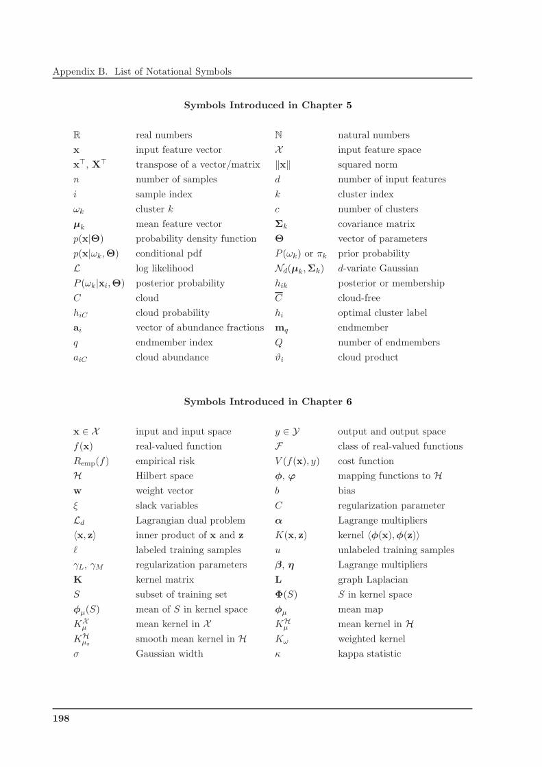
Appendix B. List of Notational Symbols
Symbols Introduced in Chapter 5
R real numbers N natural numbers
x input feature vector X input feature space
x⊤, X⊤ transpose of a vector/matrix ‖x‖ squared norm
n number of samples d number of input features
i sample index k cluster index
ωk cluster k c number of clusters
µk mean feature vector Σk covariance matrix
p(x|Θ) probability density function Θ vector of parameters
p(x|ωk,Θ) conditional pdf P (ωk) or πk prior probability
L log likelihood Nd(µk,Σk) d-variate Gaussian
P (ωk|xi,Θ) posterior probability hik posterior or membership
C cloud C cloud-free
hiC cloud probability hi optimal cluster label
ai vector of abundance fractions mq endmember
q endmember index Q number of endmembers
aiC cloud abundance ϑi cloud product
Symbols Introduced in Chapter 6
x ∈ X input and input space y ∈ Y output and output space
f(x) real-valued function F class of real-valued functions
Remp(f) empirical risk V (f(x), y) cost function
H Hilbert space φ, ϕ mapping functions to Hw weight vector b bias
ξ slack variables C regularization parameter
Ld Lagrangian dual problem α Lagrange multipliers
〈x, z〉 inner product of x and z K(x, z) kernel 〈φ(x),φ(z)〉ℓ labeled training samples u unlabeled training samples
γL, γM regularization parameters β, η Lagrange multipliers
K kernel matrix L graph Laplacian
S subset of training set Φ(S) S in kernel space
φµ(S) mean of S in kernel space φµ mean map
KXµ mean kernel in X KH
µ mean kernel in HKH
µssmooth mean kernel in H Kω weighted kernel
σ Gaussian width κ kappa statistic
198

Part VI
Summary in Spanish

Resumen
Esta Tesis aborda el problema de la deteccion de nubes en imagenes multiespectrales adquiri-
das desde satelites por instrumentos que trabajan en el rango visible e infrarrojo del espectro
electromagnetico.
Los sistemas de observacion de la Tierra observan nuestro planeta midiendo en diferentes
longitudes de onda la radiacion electromagnetica reflejada por la superficie que cruza la atmosfera
hasta el satelite. La cantidad de imagenes adquiridas todos los dıas por los instrumentos a bordo
de los satelites de observacion de la Tierra hace inevitable que muchas de estas imagenes esten
cubiertas de nubes. Se estima que mas de 60% del globo esta cubierto por nubes. De hecho,
las nubes son uno de los componentes mas importantes de la atmosfera de la Tierra y que mas
afecta a la calidad de la senal electromagnetica medida y, por tanto, tambien a las propiedades
derivadas de ella. Desde el punto de vista operativo, las nubes son la fuente mas significativa
de error para la obtencion de la reflectividad de la superficie y afectan a una amplia gama de
aplicaciones en teledetecion. Enmascarando en las imagenes las zonas afectadas por nubes, no es
necesario descartar toda la imagen. Por otro lado, la observacion de las nubes a escala mundial
es un requisito fundamental para establecer un modelo adecuado del clima de la Tierra. Por
tanto, las nubes se pueden ver como una fuente de error que hace que la imagen adquirida solo
sirva parcialmente para obtener propiedades de la cubierta terrestre, pero tambien como una
fuente de informacion que permite medir importantes parametros climatologicos. En ambos casos
es imprescindible disponer de un metodo que permita enmascarar de forma precisa las nubes
presentes en las imagenes de sensores opticos de teledeteccion. Como resultado, la deteccion
de nubes representa una importante tarea en el preprocesado de cualquier imagen optica de
teledeteccion con el fin de garantizar una maxima precision y fiabilidad en los resultados inferidos
de la explotacion de los datos.
En este contexto, esta Tesis esta tambien dirigida a cubrir el creciente interes de la comunidad
cientıfica en dos sensores a bordo de dos de los satelites de la Agencia Espacial Europea (ESA). El
primero es el MEdium Resolution Imaging Spectrometer (MERIS), instalado en ENVISAT que es
el satelite medioambiental mas grande jamas lanzado. El segundo es el Compact High Resolution
Imaging Spectrometer (CHRIS), que es un instrumento hiperespectral unico montado a bordo de
la mision de demostracion tecnologica PROBA.
El objetivo principal es el de proporcionar nuevas herramientas operativas de enmascaramiento
de nubes que proporcionen mapas con la localizacion de las nubes a partir de las propias imagenes.
Ademas, el metodo debe proporcionar mapas con la proporcion de nube para cada pıxel (en lugar
de una clasificacion binaria) para describir mejor las nubes (proporcion, tipo, altura, superficie
cubierta). Permitiendo ası la estimacion de parametros biofısicos de la superficie a partir de las
imagenes de satelite. El algoritmo de deteccion de nubes propuesto aprovecha la excepcional
resolucion espectral y radiometrica de MERIS o el gran numero de bandas espectrales de CHRIS
junto con la posicion especıfica de la longitud de onda de alguna de sus bandas (como por ejemplo
las que coinciden con las absorciones del oxıgeno o el vapor de agua atmosfericos) que permiten
mejorar la precision de la deteccion de nubes.
Para alcanzar este objetivo, diferentes tecnicas de reconocimiento de patrones y aprendizaje
automatico han sido especıficamente desarrolladas en el marco de esta Tesis para la deteccion
de nubes. Primero, se extraen de los datos caracterısticas fısicas significativas de las nubes para
proporcionar a los algoritmos unas entradas con la mejor informacion posible. A continuacion, se
propone un algoritmo de deteccion de nubes partiendo de la suposicion de que se debe explotar
la riqueza de las muestras de las imagenes analizadas aunque no se disponga de informacion de
su clase. Por lo tanto, se exploran metodos de aprendizaje no supervisado y semisupervisado. En
primer lugar, la aplicacion de metodos de agrupamiento (clustering) sobre la imagen completa
nos permite aprovechar la riqueza de la informacion de la distribucion de los datos y el alto grado
de correlacion espacial y espectral de los pıxeles de la imagen. En segundo lugar, los metodos de
aprendizaje semisupervisados ofrecen la oportunidad de explotar tambien las muestras etiquetadas
disponibles.
La validacion de los algoritmos de deteccion de nubes no es una tarea facil ya que, por lo
general, no hay medidas independientes y con la misma resolucion que informen sobre la existencia
o no de nubes en el momento de la adquisicion de la imagen. Por estas razones, se ha de realizar
un esfuerzo importante para validar los resultados usando diferentes tecnicas: por medio de un
analisis visual de las imagenes en color originales, comparando la mascara de nubes resultante
con los productos oficiales de la ESA (MERIS Level 2 Cloud Flag) y empleando algoritmos de
deteccion de cambios aplicados a series multitemporales.
Para concluir, un resultado importante de esta Tesis incluye la elaboracion de un conjunto
de directrices y recomendaciones para misiones futuras. En concreto, el estudio ha dado lugar a
una lista cualitativa de las principales cuestiones y caracterısticas fısicas que pueden mejorar la
deteccion de nubes en los sensores de teledeteccion que trabajan en el visible e infrarrojo cercano.
202
Vision General
Observacion de la Tierra
La observacion de la Tierra comprende aquellos procedimientos y metodologıas cientıficas
centradas en observar nuestro planeta por medio de la radiacion electromagnetica medida por
sensores situados en plataformas espaciales. La informacion que proporcionan estos sensores
representa escalas espaciales y temporales completamente diferentes de las obtenidas a partir de
mediciones sobre el terreno. En particular, la teledeteccion optica pasiva se basa en el estudio de
la superficie por medio de la radiacion solar reflejada por el area observada y transmitida a traves
de la atmosfera hasta llegar al sensor.
Los materiales en una escena reflejan, absorben y emiten la radiacion electromagnetica de
diferentes maneras dependiendo de su composicion molecular y su forma. La teledeteccion explota
este hecho fısico y tiene que ver con la adquisicion de informacion a corta, media o larga distancia.
La radiacion adquirida por el sensor se mide en diferentes longitudes de onda, y la consiguiente
firma espectral (espectro) se utiliza para identificar un determinado material o estimar parametros
biofısicos de la superficie. El campo de la espectroscopıa se refiere a la medicion, analisis e
interpretacion de esos espectros.
Efectos radiativos de las nubes
Sin embargo, la observacion de la Tierra a partir de datos de teledeteccion implica tener en
cuenta el acoplamiento de los efectos radiativos entre la atmosfera y la superficie. Si no hay
atmosfera alrededor de la Tierra, la radiacion solar solo se perturba cuando alcanza la superficie.
Por lo tanto, la radiacion medida proporcionarıa una representacion de la superficie e indirec-
tamente de la dinamica de la naturaleza. Sin embargo, la influencia de la atmosfera sobre la
radiacion en el visible (VIS) e infrarrojo (IR) es lo suficientemente fuerte como para modificar
la senal electromagnetica reflejada, causando la perdida o corrupcion de parte de la informacion
transportada. La interaccion de la radiacion solar con los componentes atmosfericos consiste
basicamente en procesos de absorcion y dispersion. La absorcion disminuye la intensidad de la
radiacion que llega al sensor, lo que provoca una perdida en la luminosidad del objetivo observado,
mientras que la dispersion actua principalmente modificando la direccion de propagacion.
En este escenario, las nubes son uno de los componentes mas importantes de la atmosfera de la
Tierra, y constituyen el nucleo central de este trabajo. La presencia de nubes, afecta drasticamente
a la calidad y fiabilidad de las mediciones de la senal electromagnetica y, por tanto, a la estimacion
de las propiedades de la superficie. La influencia correspondiente a las nubes depende de su tipo,
cubierta, altura y distribucion en el cielo. Por ejemplo, nubes gruesas opacas impiden la entrada
de radiacion en su camino a la superficie, mientras que nubes finas transparentes contaminan
los datos con fotones dispersados en la direccion de observacion o atenuan la senal eliminando
203
los fotones en su camino hacia el sensor. Como resultado, cualquier conjunto de imagenes de
teledeteccion requiere una deteccion de nubes precisa en las primeras etapas de procesamiento,
antes de la explotacion de los datos, para garantizar una maxima precision en los resultados
derivados. Esta es la base fundamental del enmascaramiento de nubes en la teledeteccion optica:
la deteccion de las nubes en la lınea de vision del observador con el fin de determinar la utilidad
de la senal reflejada por el objetivo.
Motivacion de la Tesis
La identificacion de las nubes en las imagenes de teledeteccion es una cuestion clave para una
amplia gama de aplicaciones de la teledeteccion, especialmente en el caso de sensores que trabajan
en el visible e infrarrojo cercano (VNIR) del espectro electromagnetico. La cantidad de imagenes
adquiridas todos los dıas por los instrumentos a bordo de los satelites de observacion de la Tierra
hace inevitable que muchas de estas imagenes presenten cubiertas nubosas, cuyo alcance depende
de la estacion y la posicion geografica de la region de estudio.
Por un lado, las nubes pueden ser vistas como una fuente de contaminacion que hace que
la imagen sea en parte inutil para evaluar las propiedades de la superficie. Sin una deteccion
exacta de las nubes, las nubes no detectadas en la escena son la fuente mas significativa de
error para estimar la reflectividad real de la superficie y, por tanto, para la recuperacion de
parametros biofısicos tanto oceanicos como terrestres. Enmascarando solo las zonas de la imagen
afectadas por nubes, no es necesario descartar toda la imagen, aumentando la usabilidad de los
datos de teledeteccion y facilitando la realizacion de estudios multitemporales. Por otro lado, las
nubes pueden ser vistas como una fuente de informacion importante para medir los parametros
climatologicos. La observacion de las nubes a escala mundial es cada vez mas importante en los
aspectos climatologicos: las nubes contribuyen de manera significativa al balance de radiacion
global con un papel importante en la reflexion de la radiacion directa, y las nubes delgadas son
tambien responsables del efecto invernadero en la atmosfera. Como resultado, la teledeteccion por
satelite de las nubes no es solo un paso en el proceso de enmascaramiento de nubes, sino tambien
un requisito para un adecuado modelado de el clima de la Tierra.
Objetivos de la Tesis
Atendiendo a las mencionadas necesidades y demandas, la presente Tesis aborda el problema
fundamental en teledeteccion de desarrollar un conjunto de herramientas operativas, precisas y
automatizadas para la discriminacion de las nubes. Podemos distinguir distintos objetivos en este
trabajo:
1. Analizar el problema de la deteccion de nubes bajo diferentes perspectivas. La natu-
raleza multidisciplinar intrınseca de este trabajo (en la interseccion entre la fısica, la ter-
modinamica, las telecomunicaciones, la informatica y el aprendizaje maquina) nos permitira
204
extraer diferentes caracterısticas para un mejor entendimiento y modelizacion del problema.
2. Entender mejor las senales proporcionadas por los espectrometros de imagen ENVISAT/
MERIS y PROBA/CHRIS. En particular, PROBA es un satelite de demostracion tec-
nologica cuyo sensor CHRIS proporciona datos mınimamente preprocesados. La adecuada
correccion y calibracion de los datos de CHRIS y MERIS es una cuestion clave para una
adecuada deteccion de las nubes y tambien para cualquier otra aplicacion.
3. Desarrollar un algoritmo de deteccion de nubes automatico, robusto y operacional. El
algoritmo debe principalmente proporcionar una mascara de nubes interpretable como la
abundancia de nube en cada pıxel.
4. Validar el algoritmo propuesto. Comparando los resultados del enmascaramiento de nubes
con productos oficiales de los diferentes satelites y con la clasificacion multi-temporal de las
cubiertas de nubes en series de imagenes.
5. Proporcionar un conjunto de directrices y recomendaciones para el desarrollo de nuevos
sensores y misiones de satelites.
Organizacion de la Tesis
Esta Tesis esta organizada en cuatro partes: (1) una profunda revision bibliografica, (2) el
desarrollo de un conjunto robusto de herramientas automatizadas para la deteccion de nubes, y
(3) la evaluacion de los algoritmos propuestos en situaciones reales:
• La primera parte del trabajo esta dedicada a una revision de los aspectos generales de
la fısica y propiedades opticas de las nubes junto con una recopilacion de los metodos de
deteccion actuales. En este primer paso se identifican los puntos fuertes y debiles de los
algoritmos mas representativos propuestos hasta la fecha.
• La segunda parte de este trabajo aborda la metodologıa propuesta para la generacion de
productos de nubes. En particular, para producir una mascara de probabilidad de nubes y
obtener conocimiento de las caracterısticas extraıdas de las nubes.
• La tercera parte del trabajo se ocupa de la validacion de la metodologıa propuesta y los
productos de nubes. Una amplia base de datos de imagenes se ha incluido en el estudio
con el fin de tener en cuenta sus diferentes caracterısticas: ubicacion geografica (latitud
/ longitud); fecha y estacion; tipo de nubes (cumulos, cirros, stratocumulus), y tipos de
superficie.
• La ultima parte del trabajo resume los objetivos conseguidos, examina las principales con-
clusiones, y proporciona recomendaciones para mejorar la deteccion de nubes en imagenes
multiespectrales para espectrometros de futuras misiones de observacion de la Tierra.
205

Teledeteccion Mediante Satelites de Observacion de la Tierra
La teledeteccion optica pasiva se basa en la radiacion solar como fuente de iluminacion. Esta
radiacion solar viaja a traves de la atmosfera terrestre antes de ser reflejada por la superficie y
de nuevo antes de llegar al sensor. Por lo tanto, la senal medida en el satelite es la radiacion
emergente del sistema tierra-atmosfera en la direccion de observacion del sensor.
La reflectividad del objeto observado es el parametro de interes, ya que caracteriza la su-
perficie independientemente de los efectos atmosfericos y las diferencias estacionales y diurnas
en la posicion solar. Sin embargo, la estimacion de la reflectividad de la superficie a partir de
la radiancia medida en el satelite (proceso conocido como correccion atmosferica) requiere una
estimacion precisa de los parametros utilizados para modelar los efectos atmosfericos y, a conti-
nuacion, compensarlos usando un buen modelo de transferencia radiativa. El principal problema
es que, para estimar los parametros atmosfericos desde los propios datos, previamente es necesaria
una deteccion de nubes precisa. Por lo tanto, la deteccion de nubes es el primer paso despues de
la reduccion del ruido y la calibracion radiometrica de los datos.
Debemos senalar aquı que el procedimiento de correccion atmosferica esta fuera del marco de
esta Tesis. Sin embargo, dado que la deteccion de nubes se lleva a cabo antes de que se realice
la correccion atmosferica, la interaccion entre la atmosfera y la radiacion se tendra en cuenta a
fin de cuantificar los efectos atmosfericos en la senal medida. Por otra parte, una formulacion
precisa de los efectos atmosfericos sobre la senal a recuperar nos permite estimar caracterısticas
utiles para discriminar las nubes de la superficie.
En el capıtulo 1, se hace una breve introduccion sobre la energıa solar, la radiacion electro-
magnetica y su interaccion con la atmosfera terrestre. Se describen los procesos de absorcion y
dispersion que afectan a la radiacion electromagnetica solar en su camino a traves de la atmosfera
hasta llegar al sensor. Se detalla la adquisicion y el modo de funcionamiento de los espectrometros
de imagen multiespectrales. Por ultimo, se incluye una breve descripcion de los sensores de satelite
ENVISAT/MERIS y PROBA/CHRIS junto con una discusion sobre las oportunidades y proble-
mas identificados que justifican la decision de estudiar en la presente Tesis la deteccion de nubes
en este tipo de sensores.
Deteccion de Nubes en Imagenes de Teledeteccion
Las nubes se pueden definir como una masa de vapor de agua condensada o partıculas de
hielo en suspension por encima de la superficie terrestre. Debido a las intensas absorciones de las
nubes en las longitudes de onda del visible e infrarrojo cercano, la mayor parte de las aplicaciones
en teledeteccion que usan datos de sensores sensibles a este rango del espectro electromagnetico
requieren la identificacion de las nubes en las imagenes. La cantidad de imagenes adquiridas a lo
largo del mundo todos los dıas por los instrumentos a bordo de los satelites de observacion de la
206
Tierra hace inevitable que muchas de estas imagenes presenten nubes, cuyo alcance depende de la
estacion y la posicion geografica de la region de estudio. De acuerdo con estimaciones de las obser-
vaciones obtenidas en el International Satellite Cloud Climatology Project (ISCCP) (Zhang et al.,
2004), la media global anual de nubosidad es de 66% aproximadamente. Otros estudios reportan
tasas mas altas de nubes en el planeta analizando los datos de una red meteorologica en todo el
mundo con un gran numero de estaciones en diferentes latitudes (Breon and Colzy, 1999).
La presencia de nubes afecta drasticamente la senal electromagnetica medida y, por tanto, a
la informacion obtenida de la superficie observada. Por ejemplo, nubes espesas opacas impiden
la entrada de radiacion hasta la superficie, mientras que nubes finas transparentes contaminan
los datos de fotones dispersados en la direccion de observacion y atenuan la senal debido a la
eliminacion de los fotones en su viaje hacia el sensor. Una cuestion importante aquı es subrayar
que, dependiendo de la aplicacion de teledeteccion, las nubes pueden ser vistas como una fuente
de contaminacion que hace que la imagen sea en parte inutil para estudiar la superficie, o como
una fuente de informacion importante para medir parametros climatologicos (Peixoto and Oort,
1992).
• Sin una mascara de nubes precisa, las nubes no detectadas en la escena son la fuente mas
significativa de error para la estimacion de la reflectividad de superficie y, por tanto, para la
recuperacion de parametros biofısicos. Enmascarando solo las zonas de la imagen afectadas
por las nubes, no es necesario descartar toda la imagen, lo que hace posible realizar estudios
multitemporales.
• La monitorizacion de las nubes a escala mundial es cada vez mas importante en estudios de
la climatologıa (las nubes contribuyen de manera significativa a la radiacion global).
La conclusion mas importante para el tema de esta Tesis es que cualquier conjunto optico de
imagenes de teledeteccion necesita llevar a cabo un proceso de deteccion de nubes en las primeras
etapas de procesamiento para garantizar la exactitud en los resultados extraıdos de las imagenes.
En el capıtulo 2, se da una breve introduccion de los tipos de nubes y las caracterısticas
clasicas utilizadas para clasificarlas. Se presentan los principales efectos de los tipos de nubes
en la radiacion electromagnetica que viaja a traves de la atmosfera terrestre y, por tanto, sus
efectos sobre el balance radiativo de la Tierra y el clima. Entonces, se describen la mayorıa de las
propiedades opticas de las nubes medibles por los sistemas de teledeteccion. Por ultimo, se lleva
a cabo un examen de los enfoques presentados en la literatura para detectar nubes, prestando
especial atencion a los algoritmos de deteccion de nubes desarrollados para los sensores estudiados
en esta Tesis.
207
Metodologıa de Deteccion de Nubes Propuesta
El objetivo principal de esta Tesis es desarrollar un algoritmo de deteccion de nubes utilizando
toda la informacion espectral proporcionada por las imagenes de los espectrometros MERIS y
CHRIS. El algoritmo de deteccion de nubes propuesto se aprovecha de la alta resolucion espectral
y radiometrica de MERIS o el elevado numero de bandas espectrales de CHRIS, ası como de la
ubicacion especıfica de algunas bandas para aumentar la precision en la deteccion de nubes, como
por ejemplo las bandas de absorcion del oxıgeno y del vapor de agua. En el capıtulo 3, se resume el
procedimiento de deteccion de nubes propuesto y se introducen brevemente los diferentes modulos
que lo constituyen.
El metodo debe ser capaz de: (i) detectar con precision las nubes, y (ii) proporcionar pro-
babilidad o abundancia de nubes en lugar de limitarse a indicar los pıxeles que presentan nubes
con una mascara binaria. El producto de abundancia de nube proporcionado no esta directa-
mente relacionado con las propiedades opticas de las nubes, como por ejemplo el espesor optico
(Kokhanovsky et al., 2007b), que generalmente se basan en modelos de transferencia radiativa.
Este producto de valor anadido permite al usuario aplicar una mascara de nubes ajustable en
funcion de las siguientes etapas de procesamiento y uso final que se le de a la imagen. Por
ejemplo, pıxeles nubosos no detectados afectan en gran medida a la recuperacion de parametros
biofısicos y a metodos basados en medidas en las longitudes de onda mas corta, como la estimacion
de aerosoles, o la estimacion de pigmentos o materia en suspension en agua, ası como a los metodos
que dependen de composiciones temporales (Saitwal et al., 2003; Ranera et al., 2005; Plummer,
2005). Un ligero sobre-enmascaramiento de los posibles pıxeles contaminados por nubes (de-
teccion de nubes conservadora) serıa preferible para garantizar un mınimo admisible en la calidad
del producto final (Guanter et al., 2008a; Kaufman et al., 2005; Martins et al., 2002), mientras
que otras aplicaciones, tales como la clasificacion de los tipos de cubiertas, son menos sensibles a
nubes delgadas, y por lo tanto, las areas con nubes muy finas no deben ser necesariamente descar-
tadas (Gomez-Chova et al., 2006f, 2007c; Camps-Valls et al., 2008a). Como resultado, el metodo
debe ser escalable y permitir diferentes niveles de enmascaramiento. Por lo tanto, se propone una
mascara probabilıstica que indique el nivel de contaminacion por nubes en cada pıxel.
Para lograr los objetivos de exactitud en la clasificacion y en el ındice de contaminacion, se
propone un esquema basado en bloques. En primer lugar, se lleva a cabo una extraccion de
caracterısticas basada en propiedades fısicas (por ejemplo, las nubes son brillantes y blancas).
Entonces, un algoritmo de clasificacion semisupervisado o no supervisado se aplica a estas ca-
racterısticas y los agrupamientos resultantes son posteriormente etiquetados como nube o libre
de nube. Por ultimo, se aplica a la imagen clasificada un algoritmo de desmezclado espectral.
Resumiendo, el procedimiento de deteccion de nubes esta constituido por los siguientes pasos:
1. Preprocesado de la Imagen: se obtiene la reflectividad de la superficie en el techo de la
atmosfera (TOA) libre de ruidos.
208

2. Extraccion de Caracterısticas: se extraen caracterısticas fısicas para aumentar la separabi-
lidad de las nubes y la superficie.
3. Segmentacion de Imagen: se aplica un algoritmo de agrupamiento no supervisado a las
caracterısticas extraıdas a fin de separar las nubes de la superficie.
4. Etiquetado de los Agrupamientos: los agrupamientos resultantes son posteriormente etique-
tados en clases geo-fısicas en funcion de sus caracterısticas extraıdas y su firma espectral.
5. Desmezclado Espectral : finalmente se aplica un algoritmo de desmezclado espectral a la
imagen segmentada con el fin de obtener un mapa de abundancias indicando el contenido
de nube por pıxel.
En los capıtulos 4, 5, y 6 se analizan los diferentes bloques en mayor detalle.
Preprocesado de la Imagen y Extraccion de Caracterısticas
Cuando se trabaja con imagenes de teledeteccion adquiridas en diferentes momentos y lugares,
una caracterıstica deseable es contar con datos independientes del sensor y de las condiciones de
adquisicion de la imagen. Esto tambien es valido para la deteccion de nubes. Por una parte,
corregir los datos de la imagen de las incertidumbres en la calibracion del sensor tiene la ventaja
de que ası los datos son independientes de las diferencias en el sensor. Por otro lado, la conversion
de datos de radiancia a reflectividad en el techo de la atmosfera tiene la ventaja de que estos
datos se corrigen de diferencias estacionales y diurnas en la posicion solar.
Una vez que los datos de la imagen se expresan en reflectancia, podemos procesar los espectros
de reflectividad con el fin de extraer caracterısticas que aumenten la separabilidad de las nubes y la
superficie. Estas caracterısticas estan inspiradas en hechos fısicos y su significado es independiente
de las diferencias en el numero, la ubicacion y el ancho de banda de los canales espectrales del
sensor, que es una caracterıstica deseable para un algoritmo de deteccion de nubes destinado a
trabajar en imagenes adquiridas por sensores multi e hiperespectrales, como MERIS y CHRIS.
Clasificacion no supervisada de las nubes
Los metodos basados en aplicar umbrales estaticos a cada pıxel de la imagen para detectar
las nubes pueden fallar debido a una cobertura parcial del pıxel, a la calibracion del sensor, a
la variacion de la respuesta espectral de las nubes con el tipo y altura de las nubes, etc. En
este contexto, el siguiente paso en nuestra metodologıa considera la utilizacion de metodos de
clasificacion para encontrar grupos similares de pıxeles en la imagen. Los metodos no supervisados
de clasificacion suponen que los datos de entrada estan organizados en una serie de grupos de
acuerdo a una determinada distancia medida en un determinado espacio (Duda and Hart, 1973).
Una revision excelente de los algoritmos de agrupamiento se puede encontrar en (Xu and Wunsch,
209
2005). En este trabajo, utilizamos el algoritmo Expectation-Maximization (Dempster et al., 1977)
para estimar los parametros de una distribucion mezcla de Gaussianas.
Clasificacion semisupervisada de las nubes
La aplicacion de metodos de agrupamiento no supervisados a toda la imagen nos permite
aprovechar la riqueza de la informacion y el alto grado de correlacion espacial y espectral de
los pıxeles de la imagen. Sin embargo, la estrategia de etiquetado de los grupos obtenidos por
metodos no supervisados se concibe para escenarios donde un usuario etiqueta manualmente los
grupos con el fin de mejorar la deteccion de nubes en estudios de casos particulares o regionales,
pero no es practico cuando se aplica a un gran numero de escenas de modo operacional. Esta
solucion esta principalmente orientada a obtener, para la imagen en cuestion, una mayor precision
en la mascara de nubes que con el enfoque estandar (que se aplica pıxel a pıxel), que produce
resultados insatisfactorios en algunos problemas crıticos, como en los bordes de las nubes o cuando
hay superficies brillantes.
Cuando el objetivo es procesar un gran numero de escenas de manera automatica debemos
recurrir a los metodos supervisados, en los que se aprende de un conjunto fiable de muestras
etiquetadas con el fin de definir una funcion de decision que clasifique correctamente los pıxeles
con nubes. Sin embargo, tıpicamente hay pocas muestras etiquetadas disponibles o que se puedan
obtener de forma regular. Nuestro objetivo es aprovechar los beneficios que muestran tanto
los metodos supervisados como no supervisados. Por esta razon, en el capıtulo 6, se exploran las
oportunidades ofrecidas por el aprendizaje semisupervisado basado en metodos kernel que explota
las pocas muestras con etiqueta y tambien la riqueza de las muestras sin etiqueta de la imagen a
clasificar.
Resultados
La tercera parte del trabajo se ocupa de la validacion de la metodologıa propuesta y de los
productos de nubes obtenidos. Una amplia base de datos de imagenes se ha incluido en el estudio
con el fin de tener en cuenta las distintas peculiaridades del problema: la ubicacion geografica,
fecha y estacion, el tipo de nube y tipos de superficie. Las imagenes seleccionadas nos permiten
validar el metodo, ya que incluyen diferentes cubiertas, vegetacion, suelos desnudos, y casos
crıticos para la deteccion de nubes como son el hielo y la nieve.
Validacion de los metodos no supervisados
La validacion de algoritmos de deteccion de nubes no es una tarea facil porque, en el caso no
supervisado (es decir, sin datos etiquetados), no suelen existir mediciones simultaneas indepen-
dientes de las nubes con la misma resolucion espacial que la imagen a clasificar. En la mayorıa
210
de los casos, el rendimiento de los algoritmos de deteccion de nubes ha sido evaluado mediante el
analisis visual de las imagenes de satelite. El ojo humano es capaz de reconocer las estructuras
de nubes en una imagen de satelite mucho mejor que cualquier algoritmo automatico, lo que jus-
tifica este enfoque de validacion. Sin embargo, el reconocimiento de las nubes puede ser difıcil en
ciertos casos (nubes delgadas, nubosidad discontinua) y esta lejos de ser operativo. Ademas, la
comparacion visual requiere una gran cantidad de trabajo tedioso, lo cual es inadecuado para una
validacion cuantitativa en un gran conjunto de datos. Por estas razones, se ha hecho un esfuerzo
significativo con el fin de validar los resultados mediante el uso de diferentes tecnicas:
• La aproximacion mas simple consiste en comparar la mascara y abundancia de nubes con
las imagenes en color. Por lo tanto, los productos resultantes son validados por inspeccion
visual de las imagenes de CHRIS y MERIS.
• En el caso de MERIS, tambien podemos comparar los resultados con los productos oficiales
de MERIS de nivel 2 ‘Cloud Flag’ (utilizado solo para la validacion, no para el entre-
namiento).
• La falta de un mapa de verdad terreno y la escasa precision mostrada por los productos
oficiales de MERIS de nivel 2 en algunas situaciones (Santer et al., 1999) impiden la vali-
dacion de la mascara de nubes en condiciones fiables. Por lo tanto, son necesarios nuevos
enfoques de validacion para poner a prueba el algoritmo de deteccion de nubes propuesto.
En particular, se propone una aproximacion multitemporal en la que pares de imagenes con
y sin nubes sobre la misma zona se utilizan para la deteccion de pıxeles con nubes medi-
ante la identificacion de pıxeles con cambios espectrales entre ambas fechas. Los pares son
seleccionados para estar cerca en el tiempo, por lo que se evitan los cambios debidos a la
evolucion temporal de la superficie. Sin embargo, las imagenes tomadas de las orbitas con
solo tres o seis dıas de diferencia presentan una importante variacion en la geometrıa de
observacion. Por lo tanto, pıxeles con cambios significativos en su composicion debido al
diferente angulo de observacion no se consideran en el metodo multi-temporal de validacion
de deteccion de nubes.
En el capıtulo 7, se presentan los resultados del metodo propuesto en el capıtulo 5.
Validacion de los metodos semisupervisados
El metodo propuesto en el capıtulo 5 ha demostrado un excelente comportamiento en los
resultados de deteccion de nubes tal como se presenta en el capıtulo 7. Sin embargo, esta aproxi-
macion es mas adecuada para estudios de casos particulares debido a su coste computacional y a la
interaccion opcional del usuario durante el proceso de etiquetado de los agrupamientos. En aplica-
ciones de deteccion de nubes operativas, se requiere metodos que clasifiquen automaticamente con
precision las nubes. Por lo tanto, los metodos supervisados o semisupervisados deberıan ser mas
211

adecuados. En el capıtulo 8 se describen los resultados del enmascaramiento de nubes obtenidos
con los nuevos metodos presentados en el capıtulo 6. Todos estos metodos son clasificadores
supervisados o semisupervisados y, por tanto, requieren un conjunto representativo de muestras
etiquetadas para entrenar y validar los modelos.
Discusion y Conclusiones
Resumen y Conclusiones
Esta Tesis presenta una nueva metodologıa con el fin de resolver el difıcil problema de la
deteccion de nubes en imagenes adquiridas por sensores de satelite multiespectrales e hiperespec-
trales que trabajan en el rango visible e infrarrojo cercano del espectro electromagnetico. Los
sensores a bordo de dos satelites de la Agencia Espacial Europea se utilizan en este trabajo: el
MEdium Resolution Imaging Spectrometer (MERIS), a bordo del satelite ENVISAT, y el ins-
trumento hiperespectral Compact High Resolution Imaging Spectrometer (CHRIS), a bordo de
PROBA.
La metodologıa propuesta identifica la ubicacion de las nubes en la imagen y produce una
abundancia de nube con el fin de cuantificar la forma en que la presencia de nubes afecta a la
medicion de espectros. El algoritmo de deteccion se basa en las caracterısticas fısicas extraıdas,
que estan destinadas a aumentar la separabilidad entre las nubes y la superficie, y se extraen de
la reflectividad en el techo de la atmosfera que pretende reducir la dependencia de la iluminacion
y las condiciones geometricas de adquisicion. Se ha hecho un importante esfuerzo para corregir
y calibrar las imagenes de los sensores seleccionados con el fin de garantizar la calidad de los
datos. En este sentido, un nuevo algoritmo se ha propuesto para el tratamiento previo de sensores
hiperespectrales, que es especialmente pertinente en el caso del sensor CHRIS.
El objetivo final ha sido el de desarrollar un conjunto de herramientas preciso y automatico
para la discriminacion de las nubes. De esta manera, dos aproximaciones diferentes se han pro-
puesto en funcion de si el algoritmo tiene que ser aplicado de forma operativa para clasificar
automaticamente un numero importante de imagenes, o el proceso de clasificacion puede ser
guiado por un operador para identificar con precision incluso los casos mas crıticos en problemas
de deteccion de nubes. Ambas aproximaciones usan, como punto de partida, un algoritmo de
agrupamiento no supervisado basado en las caracterısticas extraıdas con el fin de adaptar el en-
mascaramiento de nubes a la situacion de cada imagen, sobre todo a las condiciones atmosfericas,
el escenario de fondo, y los tipos de nubes. Este paso permite discriminar facilmente entre regiones
con y sin nubes, proporcionando un producto de abundancia de nube basado en un algoritmo de
desmezclado espectral.
En los parrafos siguientes se destacan varias observaciones y conclusiones se han extraıdo de
los diferentes modulos y algoritmos desarrollados en esta Tesis.
212

Preprocesado de la imagen. El primer paso del proceso es corregir los datos de teledeteccion
a fin de obtener una senal de radiancia en el techo de la atmosfera lo mas precisa posible. Hay
que tener en cuenta que corregir y compensar los datos de la imagen de incertidumbres en la
calibracion de los datos del sensor hace que estos datos sean independientes del sistema. Esto re-
quiere una profunda comprension de las senales proporcionadas por los espectrometros de imagen
ENVISAT/MERIS y PROBA/CHRIS para adaptar el algoritmo de deteccion de nubes, o incluso
para desarrollar nuevos algoritmos de correccion.
• El efecto sonrisa (smile effect) produce pequenas variaciones de la longitud de onda espectral
medida por cada pıxel en la direccion horizontal del sensor que tienen un gran impacto en la
caracterıstica de la absorcion de oxıgeno, que es sumamente estrecha. Por lo tanto, hemos
propuesto un nuevo algoritmo de extraccion de caracterısticas que permite la introduccion
de este desplazamiento de la respuesta espectral de MERIS en nuestra formulacion.
• PROBA es un satelite de demostracion de tecnologıa y se han desarrollado varios algorit-
mos de reduccion de ruido en esta Tesis ya que CHRIS proporciona datos mınimamente
preprocesados.
• Se ha presentado una nueva tecnica para detectar pıxeles con errores y corregirlos haciendo
uso de la informacion espacial y espectral del pıxel erroneo y sus vecinos. Aunque se trata
de una correccion cosmetica, es necesaria ya que las etapas de procesado posteriores se ven
afectadas drasticamente por estos pıxeles con valores anomalos.
• Se ha presentado una nueva tecnica para reducir el ruido coherente conocido como vertical
striping, que se encuentra normalmente en las imagenes hiperespectrales adquiridos por
sensores como CHRIS. La principal novedad de nuestra propuesta consiste en reducir el
patron de bandas verticales usando un nuevo algoritmo robusto a cambios en la superficie.
• La aproximacion propuesta de eliminacion de patrones de ruido verticales ha demostrado ser
robusta, estable, y permite modelizar con exito la dependencia del ruido con la temperatura
del sensor.
Extraccion de caracterısticas. Cuando se trabaja con imagenes de teledeteccion adquiridas
en diferentes momentos y lugares, una caracterıstica deseable es tener datos independientes de
las condiciones de adquisicion. La conversion de datos de radiancia en reflectividad en el techo
de la atmosfera tiene la ventaja de que estos datos se corrigen de diferencias en la posicion solar
estacionales y diurnas. Por otra parte, la extraccion de caracterısticas fısicas adecuadas, aumenta
la separabilidad entre las nubes y la superficie, lo que mejora la clasificacion y permite una mejor
comprension del problema.
Debemos tener en cuenta que, ademas de propiedades comunes de las nubes como ser ra-
diometricamente blancas y brillantes, una caracterıstica crıtica presentada en este trabajo es el
213

uso de las bandas de absorcion del oxıgeno atmosferico y del vapor de agua para mejorar los
resultados de la deteccion de nubes.
• La utilizacion de la absorcion atmosferica del oxıgeno para inferir la presion de las nubes, la
cual se relaciona con la altitud de las nubes, es bien conocida en estudios atmosfericos. En
este sentido, se propone una formula para extraer una caracterıstica atmosferica relacionada
directamente con el camino optico mediante el uso de la geometrıa de observacion exacta
de cada pıxel.
• La banda de absorcion del oxıgeno es muy estrecha y, a pesar de la alta resolucion espectral
y radiometrica de MERIS, las pequenas variaciones de la longitud de onda espectral de cada
pıxel tienen un gran impacto en cualquier variable derivada de la banda del oxıgeno. Como
se ha mencionado, este cambio espectral se ha tenido en cuenta con el fin de corregir el smile
effect.
• En el caso de CHRIS, la banda del oxıgeno no es tan util por el mayor ancho de banda de
los canales de CHRIS. Sin embargo, algunos modos de adquisicion de CHRIS presentan una
excelente caracterizacion de la absorcion de vapor de agua.
• La maxima absorcion de vapor de agua (940 nm) se encuentra fuera del rango de MERIS,
pero la absorcion a 900 nm sigue siendo valida para medidas relativas dentro de la misma
imagen. Por otra parte, la nieve presenta mayor absorcion que las nubes a 900 nm y este
comportamiento puede observarse en las caracterısticas extraıdas.
• Los resultados obtenidos mediante la absorcion de estas caracterısticas sugieren que serıa
ventajoso ver esas bandas incluidas en futuros sensores.
• Resumiendo, el estudio ha dado lugar a una lista cualitativa de las principales cuestiones y
caracterısticas fısicas que pueden mejorar la deteccion de nubes en los sensores de telede-
teccion que trabajan en el visible e infrarrojo cercano del espectro.
Deteccion de nubes. Un objetivo central de la Tesis ha consistido en dar un conjunto de
herramientas de deteccion de nubes para la obtencion de mapas de nubes para los datos de los
sensores seleccionados. Con el fin de lograr este objetivo, tecnicas avanzadas de reconocimiento
de patrones y de aprendizaje automatico han sido desarrolladas.
• Dos aproximaciones diferentes de deteccion de nubes se han propuesto basadas en la idea
de aprovechar las muestras sin etiqueta disponibles en las imagenes de teledeteccion.
• Inicialmente se propone una aproximacion no supervisada de deteccion de nubes basada en
metodos clasicos de reconocimiento de patrones.
214
• La aplicacion de metodos de agrupamiento no supervisados a toda la imagen nos permite
aprovechar la riqueza de la informacion y el alto grado de correlacion espacial y espectral
de los pıxeles de la imagen.
• El algoritmo EM, que se aplica a las caracterısticas extraıdas, ha demostrado una excelente
capacidad para segmentar la imagen permitiendo discriminar facilmente entre regiones con
y sin nubes.
• Se ha definido un procedimiento especıfico para etiquetar los grupos encontrados a fin de
ayudar al usuario a identificar incluso los problemas de deteccion de nubes mas crıticos.
• Se han explorado metodos de aprendizaje semisupervisados, ya que ofrecen la oportunidad
de explotar las muestras etiquetadas disponibles y la riqueza de las muestras sin etiqueta.
En este caso, hay informacion supervisada disponible y se utiliza junto con las muestras sin
etiqueta de la imagen analizada para desarrollar un clasificador que proporciona la clase de
cada pıxel, pero teniendo tambien en cuenta la distribucion de los datos de la imagen. Dado
que la distribucion de las clases esta fijada por el conjunto de entrenamiento, este metodo
puede ser aplicado automaticamente a un gran numero de escenas de modo operativo.
• Se ha propuesto una nueva familia de metodos kernel basados en kernels promedio (µ-
SVM) tomando como referencia la SVM estandar, que se utiliza como referencia de los
metodos supervisados, y la SVM Laplaciana, que se utiliza como referencia de los metodos
semisupervisados.
• Los clasificadores µ-SVM propuestos combinan la similitud entre muestras, basada en las
muestras etiquetadas del conjunto de entrenamiento, y la similitud entre agrupamientos,
basada en las muestras sin etiqueta de la imagen analizada, que se calculan en el espacio
kernel gracias a un kernel compuesto.
• Con esta aproximacion, la distribucion de las clases, estimada tıpicamente a partir de un
bajo numero de muestras etiquetadas, se adapta a la distribucion de los datos de la imagen
analizada, estimada a partir de todas las muestras sin etiqueta. Como consecuencia de ello,
el enfoque propuesto es mas robusto al sesgo en la seleccion de las muestras, que es un
problema comun en aplicaciones reales de observacion de la Tierra.
Abundancia de nubes. Una de las principales exigencias impuestas a la metodologıa pro-
puesta de deteccion de nubes era proporcionar informacion sobre la contribucion de las nubes a
los espectros medidos de los pıxeles de la imagen (para cuantificar situaciones con nubes semi-
transparentes o con cobertura parcial de un pıxel). Por lo tanto, un aspecto importante de la
metodologıa de deteccion de nubes es que proporcione un producto de abundancia de nube.
• El producto de abundancia de nubes ofrece mapas con el nivel de contaminacion de nubes
para cada pıxel en lugar de una clasificacion binaria.
215
• El producto final de nubes se obtiene combinando la abundancia de nubes, calculada con
un algoritmo de desmezclado espectral, y la probabilidad de nubes, obtenida a partir del
algoritmo de agrupamiento, por medio de una multiplicacion pıxel a pıxel.
• La aproximacion propuesta combina dos fuentes complementarias de informacion procesada
por metodos independientes: la abundancia de nubes (obtenida a partir de los espectros) y
la probabilidad de nube (obtenida a partir de las caracterısticas extraıdas), que se aproxima
a uno en los pıxeles con nubes y es cercana a cero en el resto de zonas.
• El producto de abundancia de nubes puede ser usado para describir mejor las nubes detec-
tadas (cobertura subpıxel, transparencia, tipo de nubes) y para generar mascaras de nubes
con diferentes niveles de restriccion en funcion de la aplicacion.
Aproximaciones de Validacion de los Resultados. La validacion de algoritmos de de-
teccion de nubes no es una tarea facil porque no hay una medicion independiente con la misma
resolucion espacial. Por esta razon, hay que hacer un esfuerzo importante para validar los resul-
tados mediante el uso de diferentes tecnicas.
• La aproximacion mas simple consiste en la validacion de los productos resultantes mediante
inspeccion visual, comparando la mascara de nubes y abundancia con las imagenes en color.
• En el caso de MERIS, tambien puede hacerse una comparacion con los resultados oficiales
de MERIS de nivel 2, comparando la mascara de nubes producida por el metodo presentado
en terminos de acierto en la clasificacion.
• Se ha propuesto una aproximacion multitemporal de validacion para analizar el resultado de
deteccion de nubes. Se han utilizado pares de imagenes sobre la misma zona, una cubierta
con nubes y otra sin nubes, para detectar los pıxeles con nubes mediante la identificacion
de pıxeles con un cambio espectral significativo entre ambas fechas.
• Las ventajas previstas de una deteccion precisa de nubes tambien se han demostrado con
una aplicacion de clasificacio de la cubierta terrestre a nivel subpıxel. En particular, se ha
demostrado que el desmezclado de series temporales de imagenes MERIS supera al desmez-
clado de fechas independientes.
• Tambien hemos validado los productos de abundancia y probabilidad de nube respecto a la
la probabilidad de nube proporcionada por el programa BEAM Toolbox, que es el producto
de nubes mas parecido disponible para datos de MERIS.
• En el caso de los metodos de clasificacion semisupervisados, se ha proporcionado resul-
tados mas clasicos de acierto en la clasificacion (κ y acierto promedio [%] para todos los
metodos) obtenidos utilizando etiquetas y mapas de verdad terreno para entrenar y validar
los clasificadores.
216
• Los metodos kernel de clasificacion propuestos han sido examinados en dos diferentes situa-
ciones: en primer lugar, cuando hay disponibles muestras etiquetadas para caracterizar la
imagen que debe ser clasificada y, en segundo lugar, cuando no hay muestras etiquetadas
para la imagen a ser clasificada. En este ultimo caso, una configuracion experimental se ha
propuesto con el fin de inducir y analizar el llamado sesgo en la seleccion de las muestras.
Resultados y Recomendaciones. A raız de estos criterios de validacion, una serie de expe-
rimentos se han llevado a cabo para obtener una coleccion completa de resultados. Una amplia
base de datos de imagenes se ha incluido en el estudio con el fin de tener en cuenta las distintas
peculiaridades del problema (localizacion geografica, fecha y estacion, tipos de nube y tipos de
superficie) para ambos sensores.
• Los resultados han demostrado que la aproximacion guiada por usuario clasifica con precision
los casos mas difıciles de pıxeles de nubes, especialmente cirros y nubes sobre el hielo o nieve.
• Se ha observado claras deficiencias en la mascara oficial de nubes de MERIS de nivel 2 en
las superficies mas brillantes, como suelos desnudos, hielo y nieve, que se clasifican como
nubes, y tambien se han obtenido resultados mas precisos con el metodo presentado en nubes
semitransparentes o bordes de nubes, que son incorrectamente clasificadas por el producto
oficial de la ESA.
• El algoritmo tambien ha sido validado comparandolo con una mascara de nubes basada en
la deteccion de cambios temporales. A pesar de que el metodo propuesto solo utiliza la
informacion de la imagen analizada, los resultados demuestran que nuestro metodo ofrece
una mejor discriminacion de las nubes y sus bordes. Esto permite una utilizacion mas
eficiente de las imagenes y series temporales de MERIS.
• Los histogramas del producto de abundancia de nube propuesto muestran una distribucion
de valores adecuada, que difiere en gran medida de la salida probabilıstica de la red neuronal
del programa BEAM que se concentra en torno a uno y cero, y por lo tanto proporciona
una informacion mas util para el usuario.
• Los clasificadores basados en kernels promedio (µ-SVM) producen mejores resultados que
la clasificacion de la referencia proporcionada por las SVM supervisadas y las LapSVM
semisupervisadas en todos los casos. Hay que tener en cuenta que la SVM es un caso
particular de la µ-SVM, que ademas tiene en cuenta la distribucion de datos de la imagen
con el fin de definir los grupos.
• Debido a que el tiempo de CPU consumido es relativamente bajo, los clasificadores µ-SVM
tienen una buena relacion entre el coste computacional y la precision en la clasificacion.
• Ademas, los clasificadores µ-SVM que trabajan en el espacio kernel proporcionan mejores
resultados, lo que apoya la idea de que podemos encontrar un espacio mas rico en terminos
217
de separacion de clases.
• En situaciones extremas, con un bajo numero de muestras etiquetadas, la informacion de
las muestras sin etiqueta ayuda a mejorar el comportamiento de la µ-SVM y a proporcionar
mejores resultados.
• El metodo µ-SVM basado exclusivamente en similitud entre agrupamientos no es equivalente
a una simple segmentacion de la imagen y posterior clasificacion de los centros de los grupos
con una SVM supervisada. Hemos observado que su rendimiento depende de la calidad de
la segmentacion de la imagen proporcionada por el algoritmo EM.
• En los experimentos en los que la imagen se clasifica a partir de datos de otras imagenes,
la SVM se ve drasticamente afectada por el sesgo en la seleccion de las muestras de entre-
namiento (sample selection bias), ya que se basa exclusivamente en las etiquetas de muestras
que no representan a las clases en la imagen analizada.
• Un problema comun para todos los metodos kernel es que la seleccion de los parametros
libres del kernel depende de las muestras de entrenamiento y, por tanto, se ve drasticamente
afectada por el sample selection bias.
• Los clasificadores µ-SVM basados exclusivamente en los grupos encontrados proporcionan
excelentes resultados. Sin embargo, se requiere un numero suficiente de muestras etiquetadas
para describir la distribucion de las clases (con un menor numero de muestras el grupo podrıa
ser clasificado incorrectamente).
• El mapeado propuesto es el mas robusto frente al sesgo en la seleccion de muestras debido a
que la contribucion de cada una de las muestras en la definicion del centro de masa de cada
grupo en el espacio kernel H se pesa con las probabilidades a posteriori. Esto es equivalente
a eliminar las muestras que no representan adecuadamente el agrupamiento en el espacio de
entrada, y, por tanto, la estimacion del centro del agrupamiento en H se ve menos afectada
por la seleccion de un mapeado inadecuado.
• Los resultados tambien sugieren que los clasificadores µ-SVM que promedian los kernels
con las similitud entre muestras y entre grupos son una solucion de compromiso, ya que
proporcionan buenos resultados en escenarios semisupervisado, y no estan sesgados hacia el
conjunto de entrenamiento cuando se trata con problemas con seleccion de muestras sesgadas
.
• Por ultimo, los resultados muestran una relacion inversa entre la simplicidad del modelo
(numero de vectores soporte) y la precision en la clasificacion. Los modelos excesivamente
simples ofrecen malos resultados, mientras que modelos moderadamente simples proporcio-
nan una mejor clasificacion.
218
• La principal limitacion de los metodos semisupervisados es que, aunque se benefician de la
inclusion de las muestras sin etiqueta para estimar la distribucion de datos, las etiquetas
disponibles no pueden aliviar las situaciones con un excesivo sesgo de seleccion de la mues-
tras, ya que los datos de la imagen de test a clasificar no estan bien representados en el
conjunto de entrenamiento.
• En el caso de series temporales de imagenes, el sesgo de seleccion de las muestras no es
tan crıtico (la superficie observada es la misma), y los resultados obtenidos en los expe-
rimentos son aceptables porque las distribuciones de entrenamiento y de test no difieren
significativamente.
Resumiendo, se ha propuesto una metodologıa de deteccion de nubes. La metodologıa es muy
versatil y se compone de diferentes modulos disenados especıficamente que se han formulado en
terminos de algoritmos operativos que cubren los requisitos esenciales para el proceso de deteccion
de las nubes. Estos modulos se pueden actualizar con algoritmos mas avanzados o modificarse para
adaptarse a las caracterısticas de otros sensores. En consecuencia, este procedimiento puede servir
para desarrollar un algoritmo de deteccion de nubes para otros espectrometros de imagen que
trabajen en el rango espectral VNIR con una adecuada caracterizacion espectral de las absorciones
atmosfericas, como EO1/Hyperion de la NASA, las futuras misiones de observacion de la Tierra
GMES/Sentinel-3 y EnMAP, o la propuesta FLEX del explorador de la Tierra de la ESA.
Trabajo Futuro
La lista de objetivos propuestos al comienzo de esta Tesis ha sido totalmente cubierta. Sin
embargo, la metodologıa para la deteccion de nubes presentada abre muchas direcciones futuras de
investigacion debido a su modularidad. En este sentido, nuestros proximos pasos estan vinculados
a la inclusion de modificaciones dirigidas a mejorar su robustez. Por ejemplo, la inclusion de
umbrales dinamicos podrıa ser util para encontrar las regiones a analizar, mientras que la inclusion
de informacion contextual y de textura podrıa mejorar el agrupamiento. Algunas otras lıneas de
investigacion consisten en la inclusion de la posicion del sol respecto a las nubes para encontrar
sombras.
Una importante observacion es que la metodologıa se ha limitado para usar unicamente la
informacion proporcionada por los productos de MERIS o CHRIS de nivel 1. Este requisito
previo es una de las ventajas de los metodos propuestos. Sin embargo, en los experimentos,
hemos descubierto algunas dificultades de los clasificadores automaticos para distinguir superficie
brillantes a diferentes altitudes de las nubes, como por ejemplo montanas nevadas y el hielo en
latitudes altas. Estos problemas no pueden resolverse por completo con la informacion contenida
en el rango espectral cubierto por MERIS y CHRIS, pero los sensores con canales espectrales
estrechos mas alla de 1 µm han demostrado una buena capacidad para detectar las nubes gracias
a la absorcion del vapor de agua . Por esta razon, nuestras nuevas lıneas de investigacion estan
219
vinculadas a la utilizacion de datos complementarios procedentes de diferentes sensores. Por
ejemplo, la presencia de canales en el infrarrojo termico (TIR) permite la deteccion basada en
contrastes termicos. Actualmente, estamos definiendo e implementando un sistema de deteccion
de nubes que combina la informacion procedente de los instrumentos AATSR y MERIS a bordo de
ENVISAT. La adquisicion simultanea y similar resolucion espacial permite la sinergia de MERIS
y AATSR. La inclusion de la banda de AATSR SWIR a 1.6 µm en el sistema de deteccion de
nubes es de suma importancia (McIntire and Simpson, 2002). Tambien la presencia de canales en
el rango infrarrojo termico permite la deteccion basada en contraste termico (Simpson and Gobat,
1996; Papin et al., 2002) y en la variabilidad espacial sobre el mar (Martins et al., 2002).
Por otra parte, en el rango espectral de 1.38-1.50 µm, cirros y cumulos bajos de nubes pueden
ser detectados, ya que las caracterısticas de la superficie se eliminan debido a la absorcion adicional
de radiacion solar por el vapor de agua de la atmosfera entre las nubes y la superficie (incluso
en presencia de hielo o nieve). La nueva generacion de satelites, como los GMES Sentinel 2
y 3 (European Space Agency, 2007), incluyen bandas dedicadas especıficamente definidas para
realizar una deteccion precisa de cirros. Actualmente, tambien estamos analizando las ventajas
de incluir la llamada banda de cirros (1,38 µm) en el sistema de deteccion de nubes en el marco
de los estudios preparatorios de la mision FLEX (Moreno, 2006).
Por ultimo, cabe senalar que, a pesar de que se han propuesto y desarrollado tecnicas con
aplicaciones de teledeteccion en mente, algunos algoritmos propuestos se puede aplicar a otros
campos relacionados de agrupamiento y clasificacion de datos.
Relevancia de la Tesis
La aplicabilidad de la metodologıa propuesta es crucial para completar con exito el trabajo
realizado en esta Tesis. En este sentido, debemos destacar aquı los siguientes logros.
La deteccion de nubes constituye en sı misma una oportunidad a nivel cientıfico y tecnico,
lo que ha dado lugar a importantes publicaciones en el campo. Varias publicaciones abarcan los
temas mas relevantes de esta Tesis:
• El preprocesado de datos de teledeteccion de sensores hiperespectrales y multiespectrales
ha dado lugar a diferentes algoritmos para la reduccion del ruido en (Gomez-Chova et al.,
2006a; Gomez-Chova et al., 2008) y de correccion atmosferica en (Guanter et al., 2006a,
2007, 2008a).
• El metodo propuesto ha sido probado en (Gomez-Chova et al., 2005b, 2006c, 2005a) en
imagenes hiperespectrales de CHRIS con el fin de proponer y validar las metodologıas de
deteccion de nubes en situaciones favorables de resolucion espacial (34 m) y numero de
bandas (62 canales).
• En (Gomez-Chova et al., 2005c, 2006d, 2007a) se llevo a cabo un estudio preliminar de
220

deteccion de nubes con MERIS, analizando situaciones crıticas como por ejemplo la presencia
de hielo o nieve.
• Se han empleado series temporales para la deteccion de nubes en (Gomez-Chova et al.,
2006f, 2007c), clasificacion subpıxel a traves de tecnicas de unmixing (Zurita-Milla et al.,
2007), y clasificacion de los datos de teledeteccion en (Camps-Valls et al., 2006b, 2008a).
• La teorıa de los metodos kernel utilizados en esta Tesis se basa en la labor llevada a cabo
en (Camps-Valls et al., 2004a, 2006d, 2008a).
• La utilizacion de tecnicas semisupervisadas como la LapSVM y los kernel promedio ha
sido analizada en (Gomez-Chova et al., 2007b, 2008c) y (Gomez-Chova et al., 2008a, 2009),
respectivamente.
Los conocimientos adquiridos acerca de este campo de investigacion multidisciplinar ha dado
lugar a la publicacion de tres capıtulos en libros internacionales:
• Hyperspectral Image Classification with Kernels en “Kernel Methods in Bioengineering, Sig-
nal and Image Processing” (Bruzzone et al., 2007).
• Kernel Machines in Remote Sensing Image Classification en “Intelligent Systems: Tech-
niques and Applications” (Camps-Valls et al., 2008c).
• Kernel Mean for Semi-supervised Remote Sensing Data Classification en “Kernel methods
for Remote Sensing Data Analysis” (Gomez-Chova et al., 2009).
Por ultimo, la presente Tesis se ha orientado tanto a la investigacion cientıfica como al de-
sarrollo de herramientas tecnicas innovadoras. Como consecuencia de ello, la Tesis tambien se
enmarca en tres contratos diferentes de la Agencia Espacial Europea (ESA):
• Development of CHRIS/PROBA modules for the BEAM toolbox (ESRIN Contract No.
20442/07/I-LG). Actualmente, el metodo presentado se esta aplicando al sensor CHRIS
como parte del software Basic ENVISAT Toolbox for (A)ATSR and MERIS (BEAM tool-
box1) para el tratamiento previo de datos de CHRIS. En particular, los metodos presentados
en la seccion 4.1.2 y capıtulo 5 estan siendo implementados como dos modulos independi-
entes de BEAM en los subproyectos “2.3 Noise Reduction Definition” y “2.4 Cloud Masking
Definition” del proyecto, que son gestionados por el autor de esta Tesis. La decision de la
ESA de implementar los algoritmos derivados de este trabajo en el BEAM es, sin duda,
un logro significativo y demuestra tambien el interes y la aplicabilidad de la investigacion
realizada.
1http://www.brockmann-consult.de/beam/
221
• Atmospheric Corrections for Fluorescence Signal Retrieval (ESTEC Contract No. 20882/07/
NL/LvH). El conocimiento adquirido sobre la deteccion de nubes en imagenes hiperespec-
trales durante la labor llevada a cabo en esta Tesis se aplica en este proyecto (Guanter et al.,
2008b) para definir y aplicar un enmascaramiento de nubes para el sistema FLEX. Los
pıxeles con nubes deben ser enmascarado en los estudios de fluorescencia (Gomez-Chova et al.,
2006b; Guanter et al., 2007; Guanter et al., 2007; Alonso et al., 2008; Amoros-Lopez et al.,
2008a), ya que pueden contaminar la medida de la senal de fluorescencia investigada. En
el subproyecto “3.1 Cloud screening method”, que es dirigido por el autor de esta Tesis, se
esta desarrollando un metodo para la obtencion de mascaras de nubes probabilısticas, y se
esta analizando en profundidad las mejoras esperadas asociadas a la presencia de bandas en
el SWIR que medira la plataforma FLEX.
• MERIS/AATSR Synergy Algorithms for Cloud Screening, Aerosol Retrieval, and Atmo-
spheric Correction (ESRIN Contract No. 21090/07/I-LG). La extension del trabajo de
esta Tesis para el instrumento MERIS esta siendo investigada en el marco de este proyecto
(North et al., 2008). En el metodo propuesto en este proyecto se aprovecha la informacion
combinada de ambos sensores AATSR y MERIS con el fin de mejorar los productos actuales
de nubes de los dos sensores (Gomez-Chova et al., 2008b). El autor de esta Tesis es el in-
vestigador principal de este proyecto en la Universidad de Valencia y es responsable de la
definicion de un algoritmo de deteccion de nubes que combine MERIS y AATSR. Ademas,
participa en el MERIS and AATSR Cloud Screening Working Group, que fue creado por la
ESA con el fin de aunar sus esfuerzos y utilizar los conocimientos tecnicos existentes para
desarrollar nuevos metodos de deteccion de nubes.
222

Part VII
References


References
Acarreta, J. and Stammes, P. (2005). Calibration comparison between SCIAMACHY and MERIS onboard
ENVISAT. IEEE Geoscience and Remote Sensing Letters, 2(1):31–35.
Ackerman, S., Strabala, K., Menzel, W., Frey, R., Moeller, C., and Gumley, L. (1998). Discriminating
clear sky from clouds with MODIS. Journal of Geophysical Research, 103(D24):32141–32157.
Aiazzi, B., Alparone, L., Barducci, A., Baronti, S., and Pippi, I. (2002). Estimating noise and information
for multispectral imagery. Optical Engineering, 41:656–668.
Aizerman, A., Braverman, E. M., and Rozoner, L. I. (1964). Theoretical foundations of the potential
function method in pattern recognition learning. Automation and Remote Control, 25:821–837.
Akaike, H. (1974). A new look at the statistical model identification. IEEE Transactions on Automatic
Control, 19(6):716– 723.
Alonso, L., Garcia, J., Gomez-Chova, L., Calpe-Maravilla, J., and Moreno, J. (2005). Geometric Processing
of CHRIS/Proba Images Acquired in SPARC. In Proceedings of the SPARC Final Workshop, ESRIN,
Frascati, Italy. ESA-WPP-250, ESA Publications Division.
Alonso, L., Gomez-Chova, L., Amoros-Lopez, J., Vila-Frances, J., Calpe, J., Moreno, J., and Valle-Tascon,
S. d. (2006). Study for the improvement of fluorescence remote sensing. In SENtinel-2 and FLuorescence
EXperiment (SEN2FLEX) Final Workshop. ESA WPP-271, ESA Publications Division.
Alonso, L., Gomez-Chova, L., Vila-Frances, J., Amoros-Lopez, J., Guanter, L., Calpe, J., and Moreno,
J. (2007). Sensitivity analysis of the Fraunhofer Line Discrimination method for the measurement of
chlorophyll fluorescence using a field spectroradiometer. In IEEE International Geoscience and Remote
Sensing Symposium, IGARSS’2007, pages 3756–3759, Barcelona, Spain.
Alonso, L., Gomez-Chova, L., Vila-Frances, J., Amoros-Lopez, J., Guanter, L., Calpe, J., and Moreno, J.
(2008). Improved Fraunhofer Line Discrimination Method for Vegetation Fluorescence Quantification.
IEEE Geoscience and Remote Sensing Letters. In press.
Alonso, L. and Moreno, J. (2005). Advances and Limitations in a Parametric Geometric Correction
of CHRIS/Proba Data. In 3rd CHRIS/Proba Workshop, ESRIN, Frascati, Italy. ESA-SP-593, ESA
Publications Division.
Amoros-Lopez, J., Gomez-Chova, L., Plaza, A., Plaza, J., Calpe, J., Alonso, L., and Moreno, J. (2006a).
Cloud masking in remotely sensed hyperspectral images using linear and nonlinear spectral mixture
References
analysis. In Sobrino, J. A., editor, 2nd International Symposium on Recent Advances in Quantitative
Remote Sensing: RAQRS’II, pages 90–95, Torrent, Valencia, Spain.
Amoros-Lopez, J., Gomez-Chova, L., Vila-Frances, J., Alonso, L., Calpe, J., Moreno, J., and Del Valle-
Tascon, S. (2008a). Evaluation of remote sensing of vegetation fluorescence by the analysis of diurnal
cycles. International Journal of Remote Sensing, 29(17):5423–5436.
Amoros-Lopez, J., Gomez-Chova, L., Vila-Frances, J., Calpe, J., Alonso, L., Moreno, J., and del Valle-
Tascon, S. (2006b). Study of the diurnal cycle of stressed vegetation for the improvement of fluorescence
remote sensing. In Owe, M., D’Urso, G., Neale, C. M. U., and Gouweleeuw, B. T., editors, SPIE
International Remote Sensing Symposium 2006, volume 6359, page 63590R. SPIE.
Amoros-Lopez, J., Izquierdo-Verdiguier, E., Gomez-Chova, L., Munoz-Marı, J., Rodriguez-Barreiro, J. Z.,
Camps-Valls, G., and Calpe-Maravilla, J. (2008b). Multistage robust scheme for citrus identification
from high-resolution airborne images. In Bruzzone, L., editor, SPIE International Remote Sensing
Symposium 2008, volume 7109A, pages 7109A–8. SPIE.
Amoros-Lopez, J., Vila-Frances, J., Gomez-Chova, L., Alonso, L., Guanter, L., del Valle-Tascon, S., Calpe,
J., and Moreno, J. (2007). Remote sensing of chlorophyll fluorescence for estimation of stress in vege-
tation. Recommendations for future missions. In IEEE International Geoscience and Remote Sensing
Symposium, IGARSS’2007, pages 3769–3772, Barcelona, Spain.
Antoine, D. and Chami, M. (2004). Vicarious calibration of MERIS level-1b observations: early results
obtained at the Villefranche AERONET site. In Envisat MAVT-2003 - Working meeting on MERIS and
AATSR Calibration and Geophysical Validation, ESRIN, Frascati, Italy. ESA Publications Division.
Bachmann, C., Ainsworth, T., and Fusina, R. (2005). Exploiting manifold geometry in hyperspectral
imagery. IEEE Transactions on Geoscience and Remote Sensing, 43(3):441–454.
Bachmann, C., Ainsworth, T., and Fusina, R. (2006). Improved manifold coordinate representations of
large-scale hyperspectral scenes. IEEE Transactions on Geoscience and Remote Sensing, 44(10):2786–
2803.
Barducci, A., Guzzi, D., Marcoionni, P., and Pippi, I. (2005). CHRIS-PROBA performance evaluation:
Signal-to-noise ratio, instrument efficiency and data quality from acquisitions over San Rossore (Italy)
test site. In 3rd CHRIS/Proba Workshop, ESRIN, Frascati, Italy. ESA-SP-593.
Barducci, A. and Pippi, I. (2001). Analysis and rejection of systematic disturbances in hyperspectral
remotely sensed images of the Earth. Applied Optics, 40(9):1464–1477.
Barnsley, M., Settle, J., Cutter, M., Lobb, D., and Teston, F. (2004). The PROBA/CHRIS mission: a low-
cost smallsat for hyperspectral, multi-angle, observations of the Earth surface and atmosphere. IEEE
Transactions on Geoscience and Remote Sensing, 42(7):1512–1520.
Baudin, G., Matthews, S., Bessudo, R., and Bezy, J.-L. (1996). Medium-Resolution Imaging Spectrometer
(MERIS) calibration sequence. In Descour, M. R. and Mooney, J. M., editors, Imaging Spectrometry II,
volume 2819 of Presented at the Society of Photo-Optical Instrumentation Engineers (SPIE) Conference,
pages 141–150. SPIE.
226
References
Belkin, M. and Niyogi, P. (2004). Semi-supervised learning on Riemannian manifolds. Machine Learning,
Special Issue on Clustering, 56:209–239.
Belkin, M., Niyogi, P., and Sindhwani, V. (2006). Manifold regularization: A geometric framework for
learning from labeled and unlabeled examples. Journal of Machine Learning Research, 7:2399–2434.
Berk, A., Bernstein, L. S., Anderson, G. P., Acharya, P. K., Robertson, D. C., Chetwynd, J. H., and
Adler-Golden, S. M. (1998). MODTRAN cloud and multiple scattering upgrades with application to
AVIRIS. Remote Sensing of Environment, 65(3):367–375.
Bernaerts, D., Teston, F., and Bermyn, J. (2000). PROBA (Project for Onboard Autonomy). In 5th
International Symposium on Systems and Services for Small Satellites, La Baule, France.
Bezdek, J., Li, W., Attikiouzel, Y., and Windham, M. (1997). A geometric approach to cluster validity for
normal mixtures. Soft Computing - A Fusion of Foundations, Methodologies and Applications, 1(4):166–
179.
Bezy, J.-L., Gourmelon, G., Bessudo, R., Baudin, G., Sontag, H., and Weiss, S. (1999). The ENVISAT
Medium Resolution Imaging Spectrometer (MERIS). In IEEE International Geoscience and Remote
Sensing Symposium (IGARSS 1999), volume 2, pages 1432–1434.
Bickel, S., Bruckner, M., and Scheffer, T. (2007). Discriminative learning for differing training and test
distributions. In ICML ’07: Proceedings of the 24th international conference on Machine learning, pages
81–88, New York, NY, USA. ACM.
Bottou, L., Chapelle, O., DeCoste, D., and Weston, J., editors (2007). Large Scale Kernel Machines. MIT
Press, Cambridge, MA, USA.
Breon, F. and Colzy, S. (1999). Cloud detection from the spaceborne POLDER instrument and validation
against surface synoptic observations. Journal of Applied Meteorology, 38(6):777–785.
Brockmann, C. (2006). Limitations of the application of the MERIS atmospheric correction. In Second
Working Meeting on MERIS and AATSR Calibration and Geophysical Validation (MAVT-2006), ESRIN,
Frascati, Italy. ESA SP-615, ESA Publications Division.
Brockmann, C., Kramer, U., Stelzer, K., Fournier-Sicre, V., Huot, J., Belanger, S., Fell, F., Moore, G.,
Albert, P., Pinty, B., Antoine, D., Ramon, D., Doerffer, R., and Zagolsky, F. (2002). Verification of the
MERIS level 2 products. In Envisat Validation Workshop 2002, ESRIN, Frascati, Italy. ESA Publications
Division.
Bruzzone, L., Chi, M., and Marconcini, M. (2006). A novel transductive SVM for the semisupervised classi-
fication of remote-sensing images. IEEE Transactions on Geoscience and Remote Sensing, 44(11):3363–
3373.
Bruzzone, L., Gomez-Chova, L., Marconcini, M., and Camps-Valls, G. (2007). Kernel Methods in Bioengi-
neering, Signal and Image Processing, chapter Hyperspectral Image Classification with Kernels, pages
374–398. Idea Group Publishing, Hershey, PA (USA).
Buriez, J. C., Vanbauce, C., Parol, F., Goloub, P., Herman, M., Bonnel, B., Fouquart, Y., Couvert, P.,
and Seze, G. (1997). Cloud detection and derivation of cloud properties from POLDER. International
Journal of Remote Sensing, 18(13):2785–2813.
227

References
Calpe, J., Pla, F., Vila, J., Connell, J., Marchant, J., Calleja, J., Mulqueen, M., Gomez-Chova, L., and
Vazquez, S. (2003). SMARTSPECTRA: Smart Multispectral Camera For Industrial Applications. In
Advanced Concepts for Intelligent Vision Systems (ACIVS 2003), pages 242–249.
Calpe-Maravilla, J., Gomez-Chova, L., Camps-Valls, G., Soria-Olivas, E., Martın-Guerrero, J., Alonso-
Chorda, L., and Moreno, J. (2004a). Machine learning methods for hyperspectral image analysis and
modeling. In 2nd SPECTRA Workshop: A spaceborne Earth Observation Mission to address the role of
terrestrial vegetation in the Carbon Cycle. ESA WPP-225, ESA Publications Division.
Calpe-Maravilla, J., Vila-Frances, J., Gomez-Chova, L., Ribes-Gomez, E., Munoz-Marı, J., Amoros-Lopez,
J., and Navarro, M. (2005). 2-D hyperspectral imaging systems for the retrieval of biophysical parameters.
In Proceedings of the SPARC Final Workshop, ESRIN, Frascati, Italy. ESA-WPP-250, ESA Publications
Division.
Calpe-Maravilla, J., Vila-Frances, J., Ribes-Gomez, E., Duran-Bosch, V., Munoz-Marı, J., Amoros-Lopez,
J., Gomez-Chova, L., and Tajahuerce-Romera, E. (2004b). 400- to 1000-nm imaging spectrometer
based on acousto-optic tunable filters. In Meynart, R., Neeck, S. P., and Shimoda, H., editors, SPIE
International Symposium Remote Sensing 2004, volume 5570, pages 460–471. SPIE.
Calpe-Maravilla, J., Vila-Frances, J., Ribes-Gomez, E., Duran-Bosch, V., Munoz-Marı, J., Amoros-Lopez,
J., Gomez-Chova, L., and Tajahuerce-Romera, E. (2006). 400– to 1000–nm imaging spectrometer based
on acousto-optic tunable filters. Journal of Electronic Imaging, 15(2):023001.
Camps-Valls, G., Bandos Marsheva, T. V., and Zhou, D. (2007a). Semi-supervised graph-based hyperspec-
tral image classification. IEEE Transactions on Geoscience and Remote Sensing, 45(10):3044–3054.
Camps-Valls, G. and Bruzzone, L. (2004). Regularized methods for hyperspectral image classification. In
SPIE International Symposium Remote Sensing, Gran Canaria, Spain. SPIE.
Camps-Valls, G. and Bruzzone, L. (2005). Kernel-based methods for hyperspectral image classification.
IEEE Transactions on Geoscience and Remote Sensing, 43(6):1351–1362.
Camps-Valls, G., Gomez-Chova, L., Calpe, J., Soria, E., Martın, J. D., Alonso, L., and Moreno, J. (2004a).
Robust support vector method for hyperspectral data classification and knowledge discovery. IEEE
Transactions on Geoscience and Remote Sensing, 42(7):1530–1542.
Camps-Valls, G., Gomez-Chova, L., Calpe-Maravilla, J., Munoz-Marı, J., Martın-Guerrero, J., Alonso-
Chorda, L., and Moreno, J. (2006a). Pattern Recognition: Progress, Directions and Applications, chap-
ter Hyperspectral kernel classifiers, pages 75–94. Computer Vision Center, Universitat Autonoma de
Barcelona, Barcelona, Spain.
Camps-Valls, G., Gomez-Chova, L., Calpe-Maravilla, J., Soria-Olivas, E., Martın-Guerrero, J., and Moreno,
J. (2003). Support vector machines for crop classification using hyperspectral data. In 1st Iberian
Conference on Pattern Recognition and Image Analysis, volume LNCS 2652, pages 134–141. Lecture
Notes in Computer Science. Springer-Verlag, Berlin/Heidelberg.
Camps-Valls, G., Gomez-Chova, L., Calpe-Maravilla, J., Soria-Olivas, E., Martın-Guerrero, J. D., and
Moreno, J. (2004b). Kernel methods for HyMap imagery knowledge discovery. In Bruzzone, L., editor,
SPIE International Symposium Remote Sensing 2003, volume 5238, pages 234–243. SPIE.
228
References
Camps-Valls, G., Gomez-Chova, L., Munoz-Marı, J., Alonso, L., Calpe-Maravilla, J., and Moreno, J.
(2006b). Multitemporal image classification and change detection with kernels. In Bruzzone, L., editor,
SPIE International Remote Sensing Symposium 2006, volume 6365, page 63650H. SPIE.
Camps-Valls, G., Gomez-Chova, L., Munoz-Marı, J., Rojo-Alvarez, J. L., and Martınez-Ramon, M. (2008a).
Kernel-based framework for multi-temporal and multi-source remote sensing data classification and
change detection. IEEE Transactions on Geoscience and Remote Sensing, 46(6):1822–1835.
Camps-Valls, G., Gomez-Chova, L., Munoz-Marı, J., Vila-Frances, J., Amoros-Lopez, J., and Calpe-
Maravilla, J. (2006c). Retrieval of oceanic chlorophyll concentration with relevance vector machines.
Remote Sensing of Environment, 105(1):23–33.
Camps-Valls, G., Gomez-Chova, L., Munoz-Marı, J., Vila-Frances, J., and Calpe-Maravilla, J. (2006d).
Composite kernels for hyperspectral image classification. IEEE Geoscience and Remote Sensing Letters,
3(1):93–97.
Camps-Valls, G., Gomez-Chova, L., Vila-Frances, J., Amoros-Lopez, J., Munoz-Mar, J., and Calpe-
Maravilla, J. (2005). Relevance vector machines for sparse learning of biophysical parameters. In
Bruzzone, L., editor, SPIE International Remote Sensing Symposium 2005, volume 5982, page 59820Z.
SPIE.
Camps-Valls, G., Gomez-Chova, L., Vila-Frances, J., Martın-Guerrero, J. D., Serrano-Lopez, A. J., and
Soria-Olivas, E. (2006e). Enhancing decision-based neural networks through local competition. Neuro-
computing, 69(7-9):905–908.
Camps-Valls, G., Munoz-Marı, J., Gomez-Chova, L., and Calpe, J. (2008b). Semi-supervised Support
Vector Biophysical Parameter Estimation. In IEEE International Geoscience and Remote Sensing Sym-
posium, IGARSS’2008, Boston, USA.
Camps-Valls, G., Munoz-Marı, J., Gomez-Chova, L., and Calpe-Maravilla, J. (2008c). Intelligent Systems:
Techniques and Applications, chapter Kernel Machines in Remote Sensing Image Classification, pages
199–222. Shaker Publishing BV, Maastricht, The Netherlands.
Camps-Valls, G., Rodrigo-Gonzalez, A., Munoz-Marı, J., Gomez-Chova, L., and Calpe-Maravilla, J.
(2007b). Hyperspectral Image Classification using Relevance Vector Machines with Mahalanobis kernels.
In IEEE International Geoscience and Remote Sensing Symposium, IGARSS’2007, pages 3802–3805,
Barcelona, Spain.
Camps-Valls, G., Rojo-Alvarez, J. L., and Martınez-Ramon, M., editors (2007c). Kernel Methods in
Bioengineering, Signal and Image Processing. Idea Group Publishing, Hershey, PA (USA).
Camps-Valls, G., Serrano-Lopez, A. J., Gomez-Chova, L., Martın-Guerrero, J. D., Calpe-Maravilla, J., and
Moreno, J. (2004c). Regularized RBF Networks for Hyperspectral Data Classification. In International
Conference on Image Analysis and Recognition, ICIAR2004, volume LNCS 3212, pages 429–436. Lecture
Notes in Computer Science. Springer-Verlag, Berlin / Heidelberg.
Capolsini, P., Andrefouet, S., Rion, C., and Payri, C. (2003). A comparison of Landsat ETM+, SPOT
HRV, Ikonos, ASTER, and airborne MASTER data for coral reef habitat mapping in South Pacific
islands. Can. J. Remote Sensing, 29(2):187–200.
229

References
Castelli, V. and Cover, T. (Nov 1996). The relative value of labeled and unlabeled samples in pattern
recognition with an unknown mixing parameter. Information Theory, IEEE Transactions on, 42(6):2102–
2117.
Castelli, V. and Cover, T. M. (1995). On the exponential value of labeled samples. Pattern Recogn. Lett.,
16(1):105–111.
Chang, C. (2003). Hyperspectral Imaging: Techniques for Spectral Detection and Classification. Kluwer,
Norwell, MA.
Chang, C.-C. and Lin, C.-J. (2001). LIBSVM: a library for support vector machines. Software available at
http://www.csie.ntu.edu.tw/~cjlin/libsvm.
Chapelle, O., Scholkopf, B., and Zien, A. (2006). Semi-Supervised Learning. MIT Press, Cambridge, MA,
USA, 1st edition.
Chapelle, O., Weston, J., and Scholkopf, B. (2003). Cluster kernels for semi-supervised learning. In Becker,
S., Thrun, S., and Obermayer, K., editors, NIPS 2002, volume 15, pages 585–592, Cambridge, MA, USA.
MIT Press.
Chapman, R. M. (1962). Cloud distributions and altitude profiles from satellite. Planetary Space Science,
9(1/2):70–71.
Christodoulou, C. I., Michaelides, S. C., and Pattichis, C. S. (2003). Multifeature Texture Analysis for the
Classification of Clouds in Satellite Imagery. IEEE Transactions on Geoscience and Remote Sensing,
41(11):2662–2668.
Chung, F. (1997). Spectral Graph Theory. American Mathematical Society, Providence, RI, USA.
Congalton, R. and Green, K. (1999). Assessing the Accuracy of Remotely Sensed Data: Principles and
Practices. CRC Press, Boca Raton, FL, USA, 1 edition.
Courant, R. and Hilbert, D. (1953). Methods of Mathematical Physics. Interscience Publications. John
Wiley, New York, USA.
Cover, T. M. (1965). Geometrical and statistical properties of systems of linear inequalities with application
in pattern recognition. IEEE Transactions on Electronic Computers, 14:326–334.
Cristianini, N. and Shawe-Taylor, J. (2000). An Introduction to Support Vector Machines. Cambridge
University Press, Cambridge, UK.
Cutter, M. (2004a). Review of aspects associated with the CHRIS calibration. In 2nd CHRIS/Proba
Workshop, ESRIN, Frascati, Italy. ESA SP-578, ESA Publications Division.
Cutter, M. and Johns, L. (2005a). CHRIS data format. Technical Report issue 4.2, SIRA - European Space
Agency. http://earth.esa.int/proba/.
Cutter, M. and Johns, L. (2005b). CHRIS data products – latest issue. In 3rd CHRIS/Proba Workshop,
ESRIN, Frascati, Italy. ESA-SP-593.
Cutter, M. A. (2004b). Compact high-resolution imaging spectrometer (CHRIS) design and performance.
In Shen, S. S. and Lewis, P. E., editors, Imaging Spectrometry X, volume 5546, pages 126–131. SPIE.
230

References
D’Alba, L., Brockmann, C., and Colagrande, P. (2005). MERIS Smile Effect Characterization and Correc-
tion. Technical Report 1.0, European Space Agency.
D’Almeida, G. A., Koepke, P., and Shettle, E. P. (1991). Atmospheric Aerosol, Global Climatology and
Radiative characteristics. A. Deepak, Hampton, USA.
Davies, D. and Bouldin, D. (1979). A cluster separation measure. IEEE Trans. Pattern Anal. Machine
Intell., 1(2):224–227.
Delwart, S., Bourg, L., and Huot, J.-P. (2004). MERIS 1st Year: early calibration results. In Meynart,
R., Neeck, S. P., Shimoda, H., Lurie, J. B., and Aten, M. L., editors, Sensors, Systems, and Next-
Generation Satellites VII, volume 5234 of Presented at the Society of Photo-Optical Instrumentation
Engineers (SPIE) Conference, pages 379–390. SPIE.
Delwart, S., Preusker, R., Bourg, L., Santer, R., Ramon, D., and Fischer, J. (2007). MERIS in-flight
spectral calibration. International Journal of Remote Sensing, 28(3-4):479–496.
Dempster, A. P., Laird, N. M., and Rubin, D. B. (1977). Maximum likelihood from incomplete data via
the EM algorithm. Journal of the Royal Statistical Society, Series B, 39:1–38.
Di Vittorio, A. and Emery, W. (2002). An automated, dynamic threshold cloud-masking algorithm for
daytime AVHRR images over land. IEEE Transactions on Geoscience and Remote Sensing, 40(8):1682–
1694.
Dubuisson, P., Borde, R., Dessailly, D., and Santer, R. (2003). In-flight spectral calibration of the oxygen
A-band channel of MERIS. International Journal of Remote Sensing, 24(5):1177–1182.
Duda, R. and Hart, P. (1973). Pattern classification and scene analysis. Wiley, New York, USA.
European Space Agency (2006). MERIS Product Handbook. Technical Report 2.1, European Space
Agency. http://envisat.esa.int/handbooks/meris/.
European Space Agency (2007). GMES Sentinel-3 System Requirements Document. Technical Report 1.0,
ESA/ESTEC, Noordwijk, The Netherlands.
Evgeniou, T., Pontil, M., and Poggio, T. (2000). Regularization networks and support vector machines.
Advances in Computational Mathematics, 13(1):1–50.
Fischer, J. and Grassl, H. (1991). Detection of cloud-top height from backscattered radiances within the
Oxygen A band. Part 1: Theoretical study. Journal of Applied Meteorology, 30:1245–1259.
Fomferra, N. and Brockmann, C. (2005). Beam - the ENVISAT MERIS and AATSR Toolbox. In
MERIS (A)ATSR Workshop 2005, ESRIN, Frascati, Italy. ESA SP-597, ESA Publications Division.
http://www.brockmann-consult.de/beam/.
Gadallah, F., Csillag, F., and Smith, E. (2000). Destriping multisensor imagery with moment matching.
International Journal of Remote Sensing, 21:2505–2511(7).
Gao, B.-C., Han, W., Tsay, S. C., and Larsen, N. F. (1998). Cloud Detection over the Arctic Region Using
Airborne Imaging Spectrometer Data during the Daytime. Journal of Applied Meteorology, 37:1421–
1429.
231

References
Garcia, J. and Moreno, J. (2004). Removal of noises in CHRIS/Proba images: Application to the SPARC
campaign data. In 2nd CHRIS/Proba Workshop, ESRIN, Frascati, Italy. ESA SP-578, ESA Publications
Division.
Gartner, T., Flach, P. A., Kowalczyk, A., and Smola, A. J. (2002). Multi-instance kernels. In ICML’02:
Proceedings of the Nineteenth International Conference on Machine Learning, pages 179–186, San Fran-
cisco, CA, USA. Morgan Kaufmann Publishers Inc.
Ghosh, A., Pal, N., and Das, J. (2006). A fuzzy rule based approach to cloud cover estimation. Remote
Sensing of Environment, 100:531–549.
Goetz, A., Kindel, B., Ferri, M., and Qu, Z. (2003). HATCH: results from simulated radiances, AVIRIS
and Hyperion. IEEE Transactions on Geoscience and Remote Sensing, 41(6):1215–1222.
Goetz, A., Vane, G., Solomon, J., and Rock, B. (1985). Imaging spectrometry for Earth remote sensing.
Science, 228:1147–1153.
Gomez-Chova, L. (2002). Pattern Recognition Methods for Crop Classification from Hyperspectral Remote
Sensing Images. Dissertation Com, Boca Raton, FL, USA.
Gomez-Chova, L., Alonso, L., Guanter, L., Camps-Valls, G., Calpe, J., and Moreno, J. (2006a). Modelling
spatial and spectral systematic noise patterns on CHRIS/PROBA hyperspectral data. In Bruzzone, L.,
editor, SPIE International Remote Sensing Symposium 2006, volume 6365, page 63650Z. SPIE.
Gomez-Chova, L., Alonso, L., Guanter, L., Camps-Valls, G., Calpe, J., and Moreno, J. (2008). Correction
of systematic spatial noise in push-broom hyperspectral sensors: application to CHRIS/PROBA images.
Appl. Opt., 47(28):F46–F60.
Gomez-Chova, L., Alonso-Chorda, L., Amoros-Lopez, J., Vila-Frances, J., del Valle-Tascon, S., Calpe, J.,
and Moreno, J. (2006b). Solar induced fluorescence measurements using a field spectroradiometer. In
D’Urso, G., Osann Jochum, M., and Moreno, J., editors, Earth Observation for Vegetation Monitoring
and Water Management, volume 852, pages 274–281. AIP.
Gomez-Chova, L., Amoros, J., Camps-Valls, G., Martın, J., Calpe, J., Alonso, L., Guanter, L., Fortea,
J., and Moreno, J. (2005a). Cloud detection for CHRIS/Proba hyperspectral images. In Schafer, K.,
Comeron, A., Slusser, J. R., Picard, R. H., Carleer, M. R., and Sifakis, N. I., editors, SPIE International
Remote Sensing Symposium 2005, volume 5979, page 59791Q. SPIE.
Gomez-Chova, L., Amoros, J., Camps-Valls, G., Martın, J., Calpe, J., Alonso, L., Guanter, L., Fortea, J.,
and Moreno, J. (2005b). Cloud masking scheme based on spectral, morphological, and physical features.
In 3rd CHRIS/Proba Workshop, ESRIN, Frascati, Italy. ESA SP-593, ESA Publications Division.
Gomez-Chova, L., Calpe, J., Camps-Valls, G., Martın, J. D., Soria, E., Vila, J., Alonso-Chorda, L., and
Moreno, J. (2003a). Feature selection of hyperspectral data through local correlation and SFFS for
crop classification. In IEEE International Geoscience and Remote Sensing Symposium (IGARSS 2003),
volume 1, pages 555–557, Toulouse, France.
Gomez-Chova, L., Calpe, J., Camps-Valls, G., Martın, J. D., Soria, E., Vila, J., Alonso-Chorda, L., and
Moreno, J. (2003b). Semi-supervised classification method for hyperspectral remote sensing images.
In IEEE International Geoscience and Remote Sensing Symposium (IGARSS 2003), volume 3, pages
1776–1778, Toulouse, France.
232
References
Gomez-Chova, L., Calpe, J., Camps-Valls, G., Martın, J. D., Soria, E., Vila, J., Alonso-Chorda, L., and
Moreno, J. (2004a). Robust automatic classification method for hyperspectral imagery. In Bruzzone, L.,
editor, SPIE International Symposium Remote Sensing 2003, volume 5238, pages 398–407. SPIE.
Gomez-Chova, L., Calpe, J., Martın, J. D., Soria, E., Camps-Valls, G., and Moreno, J. (2002). Semi-
supervised method for crop classification using hyperspectral remote sensing images. In 1st International
Symposium. Recent Advantages in Quantitative Remote Sensing., Torrent, Spain.
Gomez-Chova, L., Calpe, J., Soria, E., Camps-Valls, G., Martın, J. D., and Moreno, J. (2003c). CART-
based feature selection of hyperspectral images for crop cover classification. In IEEE International
Conference on Image Processing, ICIP03, volume 3, pages 589–592, Barcelona, Spain.
Gomez-Chova, L., Calpe, J., Soria, E., Moreno, J., Gonzalez, M., Alonso, L., and Martın, J. (2001).
Improvements in land surface classification with hyperspectral HyMap data at Barrax. In Final Results
Workshop on DAISEX (Digital Airborne Spectrometer Experiment), pages 249–254, Noordwijk, The
Netherlands. ESA SP-499, ESA Publications Division.
Gomez-Chova, L., Calpe-Maravilla, J., Bruzzone, L., and Camps-Valls, G. (2009). Kernel Methods for
Remote Sensing Data Analysis, chapter Mean Kernels for Semi-supervised Remote Sensing Image Clas-
sication. Wiley & Sons.
Gomez-Chova, L., Camps-Valls, G., Amoros, J., Martın, J., Calpe, J., Alonso, L., Guanter, L., Fortea,
J., and Moreno, J. (2005c). Cloud detection for MERIS multispectral images. In MERIS (A)ATSR
Workshop 2005, ESRIN, Frascati, Italy. ESA SP-597, ESA Publications Division.
Gomez-Chova, L., Camps-Valls, G., Amoros-Lopez, J., Calpe, J., Guanter, L., Alonso, L., Fortea, J.,
and Moreno, J. (2006c). Cloud probability mask for PROBA/CHRIS hyperspectral images. In IV
CHRIS/Proba Workshop. ESA Publications Division.
Gomez-Chova, L., Camps-Valls, G., Amoros-Lopez, J., Guanter, L., Alonso, L., Calpe, J., and Moreno,
J. (2006d). New cloud detection algorithm for multispectral and hyperspectral images: Application to
ENVISAT/MERIS and PROBA/CHRIS sensors. In IEEE International Geoscience and Remote Sensing
Symposium, IGARSS’2006, pages 2757 – 2760, Denver, CO, USA.
Gomez-Chova, L., Camps-Valls, G., Calpe, J., and Bruzzone, L. (2008a). Semi-Supervised Remote Sensing
Image Classification based on Clustering and Kernel Means. In IEEE International Geoscience and
Remote Sensing Symposium, IGARSS’2008, Boston, USA.
Gomez-Chova, L., Camps-Valls, G., Calpe, J., Guanter, L., and Moreno, J. (2007a). Cloud-screening
algorithm for ENVISAT/MERIS multispectral images. IEEE Transactions on Geoscience and Remote
Sensing, 45(12):4105–4118.
Gomez-Chova, L., Camps-Valls, G., Munoz-Marı, J., Calpe, J., and Moreno, J. (2008b). Cloud Screening
Methodology for MERIS/AATSR Synergy Products. In 2nd MERIS & (A)ATSR 2008 Workshop,
ESRIN, Frascati, Italy. ESA SP, ESA Publications Division.
Gomez-Chova, L., Camps-Valls, G., Munoz-Marı, J., and Calpe-Maravilla, J. (2007b). Semi-supervised
Cloud Screening with Laplacian SVM. In IEEE International Geoscience and Remote Sensing Sympo-
sium, IGARSS’2007, pages 1521–1524, Barcelona, Spain.
233

References
Gomez-Chova, L., Camps-Valls, G., Munoz-Marı, J., and Calpe-Maravilla, J. (2008c). Semisupervised
Image Classification with Laplacian Support Vector Machines. IEEE Geoscience and Remote Sensing
Letters, 5(3):336–340.
Gomez-Chova, L., Fernandez-Prieto, D., Calpe, J., and Camps-Valls, G. (2005d). Urban Monitoring at
a Regional Scale Based on MERIS and ASAR data. In MERIS (A)ATSR Workshop 2005, ESRIN,
Frascati, Italy. ESA SP-597, ESA Publications Division.
Gomez-Chova, L., Fernandez-Prieto, D., Calpe, J., E. Soria, J. V., and Camps-Valls, G. (2004b). Multispec-
tral and multitemporal sar data characterization for urban monitoring. In 3rd International workshop
on Pattern Recognition in Remote Sensing (PRRS04).
Gomez-Chova, L., Fernandez-Prieto, D., Calpe, J., Soria, E., Vila, J., and Camps-Valls, G. (2004c). Par-
tially supervised hierarchical clustering of SAR and multispectral imagery for urban areas monitoring. In
Bruzzone, L., editor, SPIE International Symposium Remote Sensing 2004, volume 5573, pages 138–149.
SPIE.
Gomez-Chova, L., Fernandez-Prieto, D., Calpe, J., Soria, E., Vila-Frances, J., and Camps-Valls, G. (2006e).
Urban monitoring using multitemporal SAR and multispectral data. Pattern Recognition Letters, Special
Issue on “Pattern Recognition in Remote Sensing”, 27(4):234–243.
Gomez-Chova, L., Zurita-Milla, R., Camps-Valls, G., Guanter, L., Clevers, J., Calpe, J., Schaepman,
M., and Moreno, J. (2006f). Multitemporal validation of an unmixing-based MERIS cloud screening
algorithm. In Sobrino, J. A., editor, 2nd International Symposium on Recent Advances in Quantitative
Remote Sensing: RAQRS’II, pages 119–124, Torrent, Valencia, Spain.
Gomez-Chova, L., Zurita-Milla, R., Camps-Valls, G., Guanter, L., Clevers, J., Calpe, J., Schaepman, M.,
and Moreno, J. (2007c). Cloud screening and multitemporal unmixing of MERIS FR data. In ENVISAT
2007 Symposium, Montreux, Switzerland. ESA SP-636, ESA Publications Division.
Gomez-Sanchis, J., Camps-Valls, G., Gomez-Chova, L., Molto, E., Cubero, S., and Blasco, J. (2008a).
Detection of rottenness caused by penicillium digitatum in citrus skin using a hyperspectral computer
vision system. In International Conference on Agricultural Engineering, AgEng2008, Crete - Greece.
Gomez-Sanchis, J., Camps-Valls, G., Molto, E., Gomez-Chova, L., Aleixos, N., and Blasco, J. (2008b).
Segmentation of hyperspectral images for the detection of rotten mandarins. In A. Campilho, M. K.,
editor, 5th International Conference, ICIAR 2008, volume LNCS 5112, pages 1071–1080. Lecture Notes
in Computer Science. Springer, Berlin / Heidelberg.
Gomez-Sanchis, J., Gomez-Chova, L., Aleixos, N., Camps-Valls, G., Montesinos-Herrero, C., Molto, E.,
and Blasco, J. (2008c). Hyperspectral system for early detection of rottenness caused by penicillium
digitatum in mandarins. Journal of Food Engineering, 89(1):80–86.
Gomez-Sanchis, J., Molto, E., Camps-Valls, G., Gomez-Chova, L., Aleixos, N., and Blasco, J. (2008d).
Automatic correction of the effects of the light source on spherical objects. an application to the analysis
of hyperspectral images of citrus fruits. Journal of Food Engineering, 85(2):191–200.
Govaerts, Y. M. and Clerici, M. (2004). Comparison of MSG/SEVIRI calibration reference with MERIS
BRF over bright desert calibration targets. In Envisat MAVT-2003 - Working meeting on MERIS and
AATSR Calibration and Geophysical Validation, ESRIN, Frascati, Italy. ESA Publications Division.
234
References
Green, R., Asner, G., Ungar, S., and Knox, R. (2008a). Nasa mission to measure global plant physiology
and functional types. In Aerospace Conference, 2008 IEEE, pages 1–7.
Green, R., Asner, G., Ungar, S., and Knox, R. (2008b). Results of the Decadal Survey HyspIRI Imaging
Spectrometer Concept Study: A High Signal-To-Noise Ratio and High Uniformity Global Mission to
Measure Plant Physiology and Functional Type. In IEEE International Geoscience and Remote Sensing
Symposium, IGARSS’2008, Boston, USA.
Gretton, A., Borgwardt, K. M., Rasch, M., Scholkopf, B., and Smola, A. (2007a). A kernel method for the
two-sample-problem. In NIPS 2006, volume 19, pages 1–8, Cambridge, MA, USA. MIT Press.
Gretton, A., Borgwardt, K. M., Rasch, M., Scholkopf, B., and Smola, A. J. (2007b). A kernel approach to
comparing distributions. In Proceedings of the Twenty-Second AAAI Conference on Artificial Intelligence
(AAAI-07), pages 1–5.
Gualtieri, J. A., Chettri, S. R., Cromp, R. F., and Johnson, L. F. (1999). Support vector machine classifiers
as applied to AVIRIS data. In Green, R., editor, 8th JPL Airborne Earth Science Workshop: JPL
Publication 99-17, page 217227.
Gualtieri, J. A. and Cromp, R. F. (1998). Support vector machines for hyperspectral remote sensing
classification. In Proceedings of the SPIE, 27th AIPR Workshop, pages 221–232, Pasadena, CA, USA.
SPIE.
Guanter, L. (2006). New algorithms for atmospheric correction and retrieval of biophysical parameters in
Earth Observation. Application to ENVISAT/MERIS data. PhD thesis, Universitat de Valencia - Estudi
General, Valencia, Spain.
Guanter, L., Alonso, L., Gomez-Chova, L., Amoros, J., Vila, J., and Moreno, J. (2007). A Method for
the Detection of Solar-Induced Vegetation Fluorescence from MERIS FR Data. In ENVISAT 2007
Symposium, Montreux, Switzerland. ESA SP-636, ESA Publications Division.
Guanter, L., Alonso, L., Gomez-Chova, L., Amoros-Lopez, J., Vila, J., and Moreno, J. (2007). Estima-
tion of solar-induced vegetation fluorescence from space measurements. Geophysical Research Letters,
34:L08401.
Guanter, L., Alonso, L., Gomez-Chova, L., and Moreno, J. (2006a). Coupled approach for spec-
tral/radiometric calibration and surface reflectance retrieval from CHRIS/PROBA data. In IV
CHRIS/Proba Workshop. ESA Publications Division.
Guanter, L., Gomez-Chova, L., Alonso, L., Amoros, J., Vila, J., and Moreno, J. (2006b). Estimation of
solar-induced vegetation fluorescence from remote sensing data acquired during the SEN2FLEX cam-
paign. In Sobrino, J. A., editor, Second Recent Advances in Quantitative Remote Sensing, RAQRS’II,
pages 826–831. Universitat de Valencia.
Guanter, L., Gomez-Chova, L., Alonso, L., Amoros, J., Vila, J., and Moreno, J. (2006c). Estimation of solar-
induced vegetation fluorescence from remote sensing data acquired during the SEN2FLEX campaign.
In Sobrino, J. A., editor, 2nd International Symposium on Recent Advances in Quantitative Remote
Sensing: RAQRS’II, pages 826–831, Torrent, Valencia, Spain.
235

References
Guanter, L., Gomez-Chova, L., and Moreno, J. (2007). Analysis of the Spatial and Temporal Variabil-
ity of Aerosol Optical Thickness and Columnar Water Vapor from MERIS Data. In ENVISAT 2007
Symposium, Montreux, Switzerland. ESA SP-636, ESA Publications Division.
Guanter, L., Gomez-Chova, L., and Moreno, J. (2008a). Coupled retrieval of aerosol optical thickness,
columnar water vapor and surface reflectance maps from ENVISAT/MERIS data over land. Remote
Sensing of Environment, 112(6):2898–2913.
Guanter, L., Segl, K., Kaufmann, H., Verhoef, W., Alonso, L., Gomez-Chova, L., Moreno, J., and Gascon,
F. (2008b). Methodology for the retrieval of vegetation chlorophyll fluorescence from space in the frame
of the FLEX mission preparatory activities. In IEEE International Geoscience and Remote Sensing
Symposium, IGARSS’2008, Boston, USA.
Hagolle, O. and Cabot, F. (2004). Absolute calibration of MERIS using natural targets. In Envisat
MAVT-2003 - Working meeting on MERIS and AATSR Calibration and Geophysical Validation, ESRIN,
Frascati, Italy. ESA Publications Division.
Hapke, B. (1993). Theory of Reflectance and Emittance Spectroscopy. Cambridge University Press.
Haykin, S. (1999). Neural Networks: A Comprehensive Foundation. Prentice Hall, Englewood Cliffs, NJ,
USA.
Hazeu, G. (2005). The Dutch Land Use Database LGN. Technical report, Alterra, Wageningen UR, The
Netherlands. http://www.lgn.nl/.
Hazeu, G. (2006). Land use mapping and monitoring in the Netherlands (LGN5). In Braun, M., editor,
Proceedings of the 2nd Workshop of the EARSeL SIG on Land Use and Land Cover, pages 323–329.
Heckman, J. J. (1979). Sample Selection Bias as a Specification Error. Econometrica, 47(1):153–161.
Heinz, D. and Chang, C.-I. (2001). Fully constrained least squares linear mixture analysis for mate-
rial quantification in hyperspectral imagery. IEEE Transactions on Geoscience and Remote Sensing,
39(3):529–545.
Howard, L. (1804). On the Modification of Clouds, 1802. The Philosophical Magazine, 16:97–107.
Huang, J., Smola, A., Gretton, A., Borgwardt, K. M., and Scholkopf, B. (2007). Correcting sample selection
bias by unlabeled data. In NIPS 2006, volume 19, pages 1–8, Cambridge, MA, USA. MIT Press.
Izquierdo-Verdiguier, E., Amoros-Lopez, J., Gomez-Chova, L., Munoz-Marı, J., Rodrıguez-Barreiro, J. Z.,
Camps-Valls, G., and Calpe-Maravilla, J. (2008). Actualizacion del SIG citrıcola de la Comunidad Va-
lenciana mediante metodos automaticos supervisados. Revista de Teledeteccion (Revista de la Asociacion
Espanola de Teledeteccion). In press.
Jackson, Q. and Landgrebe, D. (2001). An adaptive classifier design for high-dimensional data analysis with
a limited training data set. IEEE Transactions on Geoscience and Remote Sensing, 39(12):2664–2679.
Jebara, T., Kondor, R., and Howard, A. (2004). Probability Product Kernels. Journal of Machine Learning
Research, JMLR, Special Topic on Learning Theory, 5:819–844.
236

References
Joachims, T. (2003). Transductive learning via spectral graph partitioning. In Fawcett, T. and Mishra, N.,
editors, Proceeding of the International Conference on Machine Learning, ICML2003, pages 290–297,
Washington, DC USA. AAAI Press.
Jordan, M. I. (1999). Learning in Graphical Models. MIT Press, Cambridge, MA, USA, 1st edition.
Kaufman, Y., Remer, L., and Tanre, D. (2005). A critical examination of the residual cloud contamina-
tion and diurnal sampling effects on MODIS estimates of aerosol over ocean. IEEE Transactions on
Geoscience and Remote Sensing, 43(12):2886–2897.
Kaufmann, H., Guanter, L., Segl, K., Hofer, S., Foerster, K.-P., Stuffler, T., Mueller, A., Richter, R.,
Bach, H., Hostert, P., and Chlebek, C. (2008). Environmental Mapping and Analysis Program (En-
MAP) Recent Advances and Status. In IEEE International Geoscience and Remote Sensing Symposium,
IGARSS’2008, Boston, USA.
Keshava, N. (2004). Distance metrics and band selection in hyperspectral processing with applications to
material identification and spectral libraries. IEEE Transactions on Geoscience and Remote Sensing,
42(7):1552–1565.
Keshava, N. and Mustard, J. (2002). Spectral Unmixing. IEEE Signal Processing Magazine, 19(1):44–57.
Kiehl, J. T. (1992). Climate System Modeling, chapter Atmospheric general circulation modeling. Cam-
bridge University Press, Cambridge.
Kokhanovsky, A., Mayer, B., Rozanov, V., Wapler, K., Burrows, J., and Schumann, U. (2007a). The influ-
ence of broken cloudiness on cloud top height retrievals using nadir observations of backscattered solar
radiation in the oxygen A-band. Journal of Quantitative Spectroscopy & Radiative Transfer, 103:460–477.
Kokhanovsky, A., Nauss, T., Schreier, M., von Hoyningen-Huene, W., and Burrows, J. (2007b). The
Intercomparison of Cloud Parameters Derived Using Multiple Satellite Instruments. IEEE Transactions
on Geoscience and Remote Sensing, 45(1):195–200.
Kokhanovsky, A. A., Bramstedt, K., von Hoyningen-Huene, W., and Burrows, J. P. (2007c). The Inter-
comparison of Top-of-Atmosphere Reflectivity Measured by MERIS and SCIAMACHY in the Spectral
Range of 443-865 nm. IEEE Geoscience and Remote Sensing Letters, 4(2):293–296.
Kondor, R. and Jebara, T. (2003). A kernel between sets of vectors. In International Conference on
Machine Learning, ICML03.
Landgrebe, D. (2002). Hyperspectral image data analysis. Signal Processing Magazine, IEEE, 19(1):17–28.
Larsen, R., Nielsen, A. A., and Conradsen, K. (1998). Restoration of hyperspectral push-broom scanner
data. In Gudmandsen, P., editor, Proceedings of the 17th EARSeL Symposium on Future Trends in
Remote Sensing, pages 157–162. A. A. Balkema.
Leathers, R., Downes, T., and Priest, R. (2005). Scene-based nonuniformity corrections for optical and
SWIR pushbroom sensors. Opt. Express, 13(13):5136–5150.
Lee, Y., Wahba, G., and Ackerman, S. (2004). Cloud Classification of Satellite Radiance Data by Multi-
category Support Vector Machines. Journal of Atmospheric and Oceanic Technology, 21(2):159–169.
237

References
Lenoble, J. (1993). Atmospheric Radiative Transfer. A. Deepak, Hampton, USA.
Li, B., Chi, M., Fan, J., and Xue, X. (2007). Support Cluster Machine. In Ghahramani, Z., editor,
ICML’07: Proceedings of the 24th International Conference on Machine Learning, volume 227 of ACM
International Conference Proceeding Series, pages 505–512, New York, USA. ACM.
Li, J., Menzel, W., Yang, Z., Frey, R., and Ackerman, S. (2003). High-Spatial-Resolution Surface and Cloud-
Type Classification from MODIS Multispectral Band Measurements. Journal of Applied Meteorology,
42:204–226.
Liou, K. N. (2002). An Introduction to Atmospheric Radiation. Academic Press, Hampton, USA, 2nd
edition.
Mak, B., Kwok, J., and Ho, S. (2004). A study of various composite kernels for kernel eigenvoice speaker
adaptation. In IEEE International Conference on Acoustics, Speech, and Signal Processing, ICASSP04,
volume 1, pages 325–8. IEEE.
Martins, J., Tanre, D., Remer, L. Kaufman, Y., Mattoo, S., and Levy, R. (2002). MODIS cloud screen-
ing for remote sensing of aerosols over oceans using spatial variability. Geophysical Research Letters,
29(12):8009.
Martiny, N., Santer, R., and Smolskaia, I. (2005). Vicarious calibration of MERIS over dark waters in the
near infrared. Remote Sensing of Environment, 94(4):475–490.
Mazzoni, D., Garay, M., Davies, R., and Nelson, D. (2007). An operational MISR pixel classifier using
support vector machines. Remote Sensing of Environment, 107(1/2):149–158.
McIntire, T. and Simpson, J. (2002). Arctic sea ice, cloud, water, and lead classification using neural
networks and 1.6 µm data. IEEE Transactions on Geoscience and Remote Sensing, 40(9):1956–1972.
Mercer, J. (1905). Functions of positive and negative type and their connection with the theory of integral
equations. Philosophical Transactions of the Royal Society of London, CCIX(A456):215–228.
Merchant, C., Harris, A., Maturi, E., and MacCallum, S. (2005). Probabilistic physically-based cloud
screening of satellite infra-red imagery for operational sea surface temperature retrieval. Quart. J. Royal
Met. Soc., 131:2735–2755.
Merheim-Kealy, P., Huot, J. P., and Delwart, S. (1999). The MERIS ground segment. International
Journal of Remote Sensing, 20:1703–1712.
MERIS Quality Working Group (2006). MERIS Products Quality Status Re-
port (MEGS7.4 and IPF 5). Technical Report issue 1, European Space Agency.
http://earth.esa.int/pcs/envisat/meris/documentation/.
Mlsna, P. and Becker, T. (2006). Striping artifact reduction in lunar orbiter mosaic images. In IEEE
Southwest Symposium on Image Analysis and Interpretation, pages 95–99.
Moreno, J. (2006). Fluorescence Explorer (FLEX): mapping vegetation photosynthesis from space. In
Sobrino, J. A., editor, Second Recent Advances in Quantitative Remote Sensing, RAQRS’II, pages 832–
837. Universitat de Valencia.
238

References
Moreno et al., J. (2005). The SPectra bARrax Campaign (SPARC): Overview of the activities. In Proceed-
ings of the SPARC Final Workshop, ESRIN, Frascati, Italy. ESA-WPP-250, ESA Publications Division.
Mouroulis, P., Green, R. O., and Chrien, T. G. (2000). Design of pushbroom imaging spectrometers for
optimum recovery of spectroscopic and spatial information. Applied Optics, 39:2210–2220.
Muller, K.-R., Mika, S., Ratsch, G., and Tsuda, K. (2001). An introduction to kernel-based learning
algorithms. IEEE Transactions on Neural Networks, 12(2):181–201.
Munoz-Marı, J., Camps-Valls, G., Gomez-Chova, L., and Calpe-Maravilla, J. (2007). Combination of
one-class remote sensing image classifiers. In IEEE International Geoscience and Remote Sensing Sym-
posium, IGARSS’2007, pages 1509–1512, Barcelona, Spain.
Munoz-Marı, J., Gomez-Chova, L., Camps-Valls, G., and Calpe-Maravilla, J. (2008). Image classification
with semi-supervised support vector domain description. In Bruzzone, L., editor, SPIE International
Remote Sensing Symposium 2008, volume 7109A, pages 7109A–11. SPIE.
Murtagh, F., Barreto, D., and Marcello, J. (2003). Decision Boundaries Using Bayes Factors: The Case of
Cloud Masks. IEEE Transactions on Geoscience and Remote Sensing, 41(12):2952–2958.
NASA Facts (1999). Clouds and the Energy Cycle. Technical Report NF-207, NASA, Goddard Space
Flight Center, Maryland, USA.
Naud, C., Baum, B., Bennarzt, R., Fischer, J., Frey, R., Menzel, P., Muller, J., Preusker, R., and Zhang, H.
(2003). Inter-comparison of MERIS, MODIS and MISR Cloud Top Heights. In MERIS User Workshop
2003, ESRIN, Frascati, Italy. ESA SP-549, ESA Publications Division.
North, P., Brockmann, C., Fischer, J., Gomez-Chova, L., Grey, W., Moreno, J., Preusker, R., and Regner,
P. (2008). MERIS/AATSR Synergy Algorithms for Cloud Screening, Aerosol Retrieval and Atmospheric
Correction. In 2nd MERIS & (A)ATSR 2008 Workshop, ESRIN, Frascati, Italy. ESA SP, ESA Publi-
cations Division.
Othman, H. and Qian, S.-E. (2006). Noise reduction of hyperspectral imagery using hybrid spatial-spectral
derivative-domain wavelet shrinkage. IEEE Transactions on Geoscience and Remote Sensing, 44(2):397–
408.
Papin, C., Bouthemy, P., and Rochard, G. (2002). Unsupervised segmentation of low clouds from infrared
METEOSAT images based on a contextual spatio-temporal labeling approach. IEEE Transactions on
Geoscience and Remote Sensing, 40(1):104–114.
Peixoto, J. P. and Oort, A. H. (1992). Physics of Climate. American Institute of Physics, New York, USA.
Pezoa, J. E., Hayat, M. M., Torres, S. N., and Rahman, M. S. (2006). Multimodel Kalman filtering for
adaptive nonuniformity correction in infrared sensors. J. Opt. Soc. Am. A, 23(6):1282–1291.
Platnick, S., King, M., Ackerman, S., Menzel, W., Baum, B., Riedi, J., and Frey, R. (2003). The MODIS
Cloud Products: Algorithms and Examples From Terra. IEEE Transactions on Geoscience and Remote
Sensing, 41(2):459–473.
Plaza, A. and Chang, C.-I. (2006). Impact of initialization on design of endmember extraction algorithms.
IEEE Transactions on Geoscience and Remote Sensing, 44(11):3397–3407.
239

References
Plummer, S. (2005). Establishing the GLOBCARBON Cloud Detection System over Land for the Along
Track Scanning Radiometer (ATSR) Sensor Series. In MERIS (A)ATSR Workshop 2005, ESA SP-597,
ESA Special Publication.
Pratt, W. K. (2001). Digital Image Processing: PIKS Inside, 3rd Edition. John Wiley & Sons, Inc, New
York, USA.
Preusker, R., Huenerbein, A., and Fischer, J. (2006). Cloud detection with MERIS using oxygen absorption
measurements. Geophysical Research Abstracts, 8:09956.
Ramon, D., Cazier, L., and Santer., R. (2003). The surface pressure retrieval in the MERIS O2 absorp-
tion: validation and potential improvements. In IEEE International Geoscience and Remote Sensing
Symposium, IGARSS’2003, volume 5, pages 3126–3128, Toulouse, France.
Ramon, D., Santer, R., and Dubuisson, P. (2003). MERIS in-flight spectral calibration in O2 absorption
using surface pressure retrieval. In Huang, H.-L., Lu, D., and Sasano, Y., editors, Optical Remote
Sensing of the Atmosphere and Clouds III, volume 4891 of Presented at the Society of Photo-Optical
Instrumentation Engineers (SPIE) Conference, pages 505–514. SPIE.
Ramon, D., Santer, R., and Dubuisson, P. (2004). Surface pressure product accuracy with respect to cloud
flagging. In Envisat MAVT-2003 - Working meeting on MERIS and AATSR Calibration and Geophysical
Validation, ESRIN, Frascati, Italy. ESA Publications Division.
Ranera, F., Plummer, S., and Arino, O. (2005). A pragmatic solution for cloud detection and removal in
MERIS L1B data. In MERIS (A)ATSR Workshop 2005, page 54.1, ESRIN, Frascati, Italy. ESA SP-597,
ESA Publications Division.
Rast, M., Bezy, J., and Bruzzi, S. (1999). The ESA Medium Resolution Imaging Spectrometer MERIS: a
review of the instrument and its mission. International Journal of Remote Sensing, 20(9):1681–1702.
Ren, H. and Chang, C.-I. (2003). Automatic spectral target recognition in hyperspectral imagery. IEEE
Transactions on Aerospace and Electronic Systems, 39(4):1232–1249.
Renzullo, L. (2004). Radiometric Processing of Multitemporal Sequences of Satellite Imagery for Surface
Reflectance Retrievals in Change Detection Studies. PhD thesis, Curtin University of Technology, Curtin,
USA.
Richards, J. A. and Jia, X. (1999). Remote Sensing Digital Image Analysis. An Introduction. Springer-
Verlag, Berlin, Heidelberg, Germany, 3rd edition.
Rissanen, J. (1986). Stochastic Complexity and Modeling. Annals of Statistics, 14(3):1080–1100.
Rossow, W. B. (1993). Clouds Atlas of Satellite Observations Related to Global Change, chapter Clouds.
Cambridge University Press, Cambridge.
Saitwal, K., Azimi-Sadjadi, M., and Reinke, D. (2003). A multichannel temporally adaptive system for
continuous cloud classification from satellite imagery. IEEE Transactions on Geoscience and Remote
Sensing, 41(5):1098–1104.
240
References
Salomonson, V., Barnes, W., Maymon, P., Montgomery, H., and Ostrow, H. (1989). MODIS: advanced
facility instrument for studies of the Earth as a system. IEEE Transactions on Geoscience and Remote
Sensing, 27(2):145–153.
Santer, R., Carrere, V., Dessailly, D., Dubuisson, P., and Roger, J. (1997). MERIS Algorithm Theoretical
Basis Document (ATBD 2.17). Pixel Identification. Technical Report issue 4, European Space Agency.
http://envisat.esa.int/instruments/meris/atbd/.
Santer, R., Carrere, V., Dubuisson, P., and Roger, J. C. (1999). Atmospheric correction over land for
MERIS. International Journal of Remote Sensing, 20(9):1819–1840.
Saunders, R. W. and Kriebel, K. T. (1988). An improved method for detecting clear sky and cloudy sky
radiances from AVHRR data. International Journal of Remote Sensing, 9:123–150. errata IJRS 9,
1393-1394.
Schaepman, M., Green, R., Ungar, S., Curtiss, B., Boardman, J., Plaza, A., Gao, B.-C., Kokaly, R.,
Miller, J., Jacquemoud, S., Ben-Dor, E., Clark, R., Davis, C., Dozier, J., Goodenough, D., Roberts, D.,
and Goetz, A. (2006). The future of imaging spectroscopy - prospective technologies and applications.
In IEEE International Geoscience and Remote Sensing Symposium, IGARSS’2006, pages 2005–2009,
Denver, CO, USA.
Scholkopf, B. (1997). Support Vector Learning. R. Oldenbourg Verlag, Munich.
Scholkopf, B. and Smola, A. (2001). Learning with Kernels – Support Vector Machines, Regularization,
Optimization and Beyond. MIT Press Series, Cambridge, MA, USA.
Settle, J. and Cutter, M. (2005). HDFclean V2: A program for reprocessing images captured by the CHRIS
hyperspectral imager. http://earth.esa.int/proba/.
Shahshahani, B. and Landgrebe, D. (1994). The effect of unlabeled samples in reducing the small sample
size problem and mitigating the Hughes phenomenon. IEEE Transactions on Geoscience and Remote
Sensing, 32(5):1087–1095.
Shawe-Taylor, J. and Cristianini, N. (2004). Kernel Methods for Pattern Analysis. Cambridge University
Press, Cambridge, MA, USA.
Shimodaira, H. (2000). Improving predictive inference under covariate shift by weighting the log-likelihood
function. Journal of Statistical Planning and Inference, 90(2):227–244.
Simpson, J., Schmidt, A., and Harris, A. (1998). Improved Cloud Detection in Along Track Scanning
Radiometer (ATSR) Data over the Ocean. Remote Sensing of Environment, 65(1):1–24.
Simpson, J. J. and Gobat, J. I. (1996). Improved Cloud Detection for Daytime AVHRR Scenes over Land.
Remote Sensing of Environment, 55(1):21 – 49.
Sinha, K. and Belkin, M. (2008). The value of labeled and unlabeled examples when the model is imperfect.
In NIPS 2007, volume 20, Cambridge, MA, USA. MIT Press.
Soria-Olivas, E., Martın-Guerrero, J., Camps-Valls, G., Serrano-Lopez, A., Calpe-Maravilla, J., and
Gomez-Chova, L. (2003). A low-complexity fuzzy activation function for artificial neural networks.
IEEE Transactions on Neural Networks, 14(6):1576–1579.
241
References
Srivastava, A. N. and Stroeve, J. (2003). Onboard detection of snow, ice, clouds and other geophysical pro-
cesses using kernel methods. In 12th International Conference on Machine Learning (ICML): Machine
Learning Technologies for Autonomous Space Applications Workshop, Washington, DC, USA.
Stephens, G. (2003). The Useful Pursuit of Shadows. American Scientist, 91:442–449.
Stoll, M., Buschmann, C., Court, A., Laurila, T., Moreno, J., and Moya, I. (2003). The FLEX-Fluorescence
Explorer mission project: motivations and present status of preparatory activities. In IEEE Int. Geo-
science and Remote Sensing Symposium, IGARSS03, volume 1, pages 585–587.
Stuffler, T., Kaufmann, C., Hofer, S., Forster, K. P., Schreier, G., Mueller, A., Eckardt, A., Bach, H.,
Penne, B., Benz, U., and Haydn, R. (2007). The EnMAP hyperspectral imager – An advanced optical
payload for future applications in Earth observation programmes. Acta Astronautica, 61(1-6):115–120.
Sugiyama, M., Krauledat, M., and Muller, K.-R. (2007). Covariate shift adaptation by importance weighted
cross validation. Journal of Machine Learning Research, 8:985–1005.
Sugiyama, M. and Muller, K.-R. (2005). Input-Dependent Estimation of Generalization Error under Co-
variate Shift. Statistics & Decisions, 23(4):249–279.
Sugiyama, M., Suzuki, T., Nakajima, S., Kashima, H., von Bunau, P., and Kawanabe, M. (2008). Direct
importance estimation for covariate shift adaptation. Annals of the Institute of Statistical Mathematics,
60(4). In press.
Sun, J.-T., Zhang, B.-Y., Chen, Z., Lu, Y.-C., Shi, C.-Y., and Ma, W. (2004). GE-CKO: A method to
optimize composite kernels for web page classification. In IEEE/WIC/ACM International Conference
on Web Intelligence, WI04, volume 1, pages 299–305. IEEE.
Szummer, M. and Jaakkola, T. (2002). Partially labeled classification with Markov random walks. In et al.,
T. D., editor, NIPS 2001, volume 14, pages 945–952, Cambridge, MA, USA. MIT Press.
Tanre, D., Herman, M., Deschamps, P., and de Leffe, A. (1979). Atmospheric modeling for space measure-
ments of ground reflectance, including bidirectional properties. Applied Optics, 18(21):3587–3594.
Theuwissen, A. (1995). Solid-State Imaging with Charge-Coupled Devices. Kluwer Academic, Boston, MA,
USA.
Thuillier, G., Herse, M., Labs, D., Foujols, T., Peetermans, W., Gillotay, D., Simon, P. C., and Mandel, H.
(2003). The solar spectral irradiance from 200 to 2400 nm as measured by the SOLSPEC spectrometer
from the ATLAS and EURECA missions. Solar Physics, 214:1–22.
Tian, B., Shaikh, M., Azimi, M., Haar, T., and Reinke, D. (1999). A study of cloud classification with neural
networks using spectral and textural features. IEEE Transactions on Neural Networks, 10(1):138–151.
Tikhonov, A. and Arsenin, V. (1977). Solutions of ill-posed problems. W.H. Winston, Washington, DC,
USA.
Tikhonov, A. N. (1963). Regularization of incorrectly posed problems. Sov. Math. Dokl., 4:1624–1627.
Torres, S. N., Pezoa, J. E., and Hayat, M. M. (2003). Scene-Based Nonuniformity Correction for Focal
Plane Arrays by the Method of the Inverse Covariance Form. Appl. Opt., 42(29):5872–5881.
242

References
Torres Arriaza, J. A., Guindos Rojas, F., Peralta Lopez, M., and Canton, M. (2003). An Automatic Cloud-
Masking System Using Backpro. Neural Nets for AVHRR Scenes. IEEE Transactions on Geoscience
and Remote Sensing, 41(4):826–831.
Tsang, I. W. and Kwok, J. T. (2007). Large-scale sparsified manifold regularization. Advances in Neural
Information Processing Systems, 19.
Ungar, S., Pearlman, J., Mendenhall, J., and Reuter, D. (2003). Overview of the Earth Observing One
(EO-1) mission. IEEE Transactions on Geoscience and Remote Sensing, 41(6):1149–1159.
Vapnik, V. (2000). The Nature of Statistical Learning Theory. Springer, New York, USA, 2nd edition.
Vapnik, V. and Chervonenkis, A. (1964). A note on one class of perceptrons. Automation and Remote
Control, 25.
Vapnik, V. N. (1998). Statistical Learning Theory. John Wiley & Sons, New York, USA.
Vermote, E. F., Tanre, D., Deuze, J. L., Herman, M., and Morcrette, J. J. (1997). Second Simulation of the
Satellite Signal in the Solar Spectrum, 6S: An overview. IEEE Transactions on Geoscience and Remote
Sensing, 35:675–686.
Vila, J., Calpe, J., Pla, F., Gomez-Chova, L., Connell, J., Marchant, J., Calleja, J., Mulqueen, M., Munoz,
J., and Klaren, A. (2005). Smartspectra: Applying multispectral imaging to industrial environments.
Real-Time Imaging, 11(2):85–98.
Vila-Frances, J., Amoros-Lopez, J., Alonso, L., Gomez-Chova, L., Calpe, J., del Valle-Tascon, S., and
Moreno, J. (2006a). Vegetation’s fluorescence spectrum and Kautsky effect measurements under natural
solar illumination. In Sobrino, J. A., editor, Second Recent Advances in Quantitative Remote Sensing,
RAQRS’II, pages 985–990. Universitat de Valencia.
Vila-Frances, J., Amoros-Lopez, J., Gomez-Chova, L., Alonso-Chorda, L., Guanter, L., Moreno, J., and del
Valle, S. (2007). Optimisation of the overpass time for remote sensing of vegetation fluorescence by the
analysis of diurnal cycles. In 3rd International Workshop on Remote Sensing of Vegetation Fluorescence.
ESA Publications Division.
Vila-Frances, J., Calpe-Maravilla, J., Munoz-Marı, J., Gomez-Chova, L., Amoros-Lopez, J., Ribes-Gomez,
E., and Duran-Bosch, V. (2006b). Configurable-bandwidth imaging spectrometer based on an acousto-
optic tunable filter. Review of Scientific Instruments, 77(7):073108.
Vila-Frances, J., Ribes-Gomez, E., Ibanez-Lopez, C., Gomez-Chova, L., Munoz-Marı, J., Amoros-Lopez, J.,
and Calpe-Maravilla, J. (2005). Configurable bandwidth imaging spectrometer based on acousto-optic
tunable filter. In Sliwinski, A., Reibold, R., and Voloshinov, V. B., editors, SPIE International Congress
on Optics and Optielectronics 2005, volume 5953, page 59530S. SPIE.
Wang, M. and Shi, W. (2006). Cloud Masking for Ocean Color Data Processing in the Coastal Regions.
IEEE Transactions on Geoscience and Remote Sensing, 44(11):3196–3105.
Weston, J., Leslie, C., Ie, E., Zhou, D., Elisseeff, A., and Noble, W. S. (2005). Semi-supervised protein
classification using cluster kernels. Bioinformatics, 21(15):3241–3247.
243

References
Xu, R. and Wunsch, D., I. (May 2005). Survey of clustering algorithms. IEEE Transactions on Neural
Networks, 16(3):645–678.
Yamamoto, G. and Wark, D. Q. (1961). Discussion of the letter by R. A. Hanel: Determination of cloud
altitude from a satellite. Journal of Geophysical Research, 66:3596.
Yang, Y., Di Girolamo, L., and Mazzoni, D. (2007). Selection of the automated thresholding algorithm
for the Multi-angle Imaging SpectroRadiometer Radiometric Camera-by-Camera Cloud Mask over land.
Remote Sensing of Environment, 107(1/2):159–171.
Yhann, S. R. and Simpson, J. J. (1995). Application of neural networks to AVHRR cloud segmentation.
IEEE Transactions on Geoscience and Remote Sensing, 33(3):590–604.
Zhang, Y., Rossow, W. B., Lacis, A. A., Oinas, V., and Mishchenko, M. I. (2004). Calculation of radiative
fluxes from the surface to top of atmosphere based on ISCCP and other global data sets: Refinements
of the radiative transfer model and the input data. Journal of Geophysical Research, 109(D19):D19105.
Zhou, S. and Chellappa, R. (2006). From sample similarity to ensemble similarity: probabilistic distance
measures in reproducing kernel Hilbert space. IEEE Transactions on Pattern Analysis and Machine
Intelligence, 28(6):917–929.
Zhu, X. (2005). Semi-supervised learning literature survey. Technical Report 1530,
Computer Sciences, University of Wisconsin-Madison, USA. Online document:
http://www.cs.wisc.edu/~jerryzhu/pub/ssl_survey.pdf. Last modified on June 24, 2007.
Zhu, X. and Ghahramani, Z. (2002). Learning from labeled and unlabeled data with label propagation.
Technical Report CMU-CALD-02-107, Carnegie Mellon University.
Zurita-Milla, R., Gomez-Chova, Clevers, J., Schaepman, M., and Camps-Valls, G. (2007). Multitemporal
Unmixing of MERIS FR Data. In Schaepman, M., Liang, S., Groot, N., and Kneubuhler, M., editors, 10th
Intl. Symposium on Physical Measurements and Spectral Signatures in Remote Sensing (ISPMSRS07),
volume XXXVI, Part 7/C50, pages 238–243. Intl. Archives of the Photogrammetry, Remote Sensing and
Spatial Information Sciences.
244


