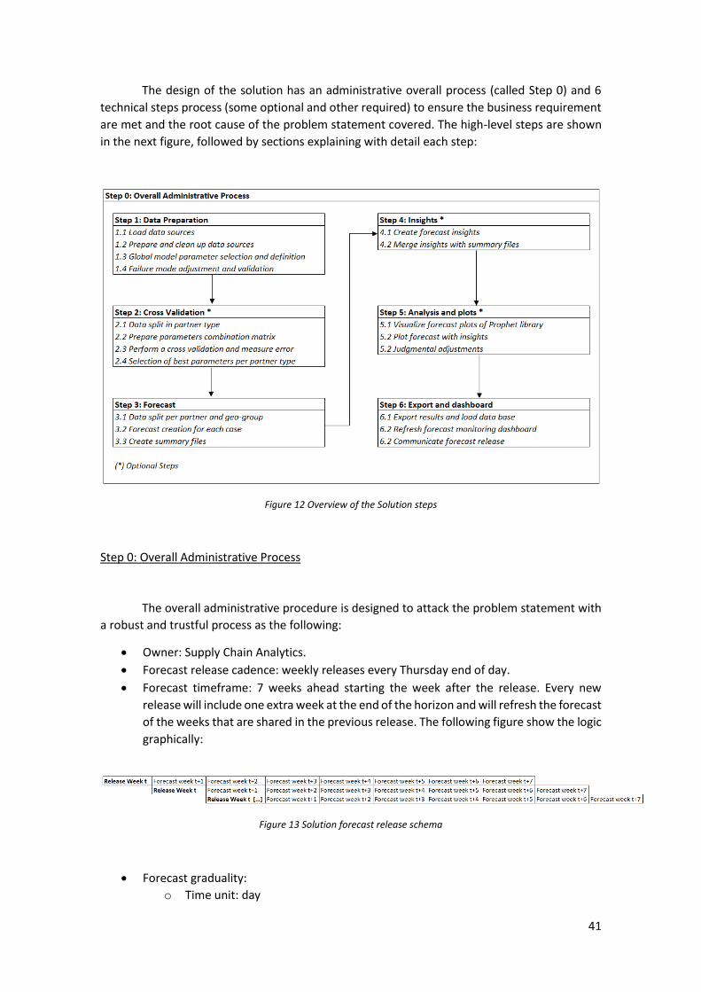
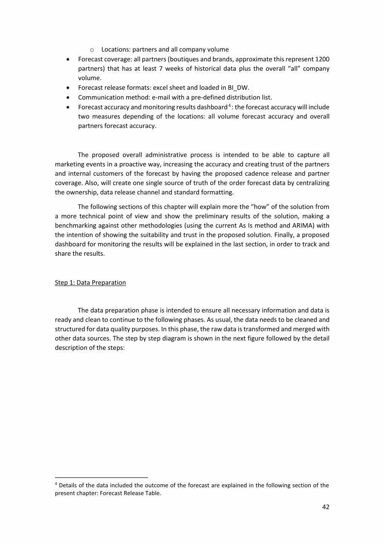
Automated Time Series Demand Forecast for

Luxury Fashion Online Retail Company

Leonel Murillo Alfaro

Internship report presented as partial requirement for

obtaining the Master’s degree in Advanced Analytics

III

NOVA Information Management School

Instituto Superior de Estatística e Gestão de Informação

Universidade Nova de Lisboa

AUTOMATED TIME SERIES DEMAND FORECAST FOR LUXURY

FASHION ONLINE RETAIL COMPANY

by

Leonel Murillo Alfaro

M20170005

Internship report presented as partial requirement for obtaining the Master’s degree in

Advanced Analytics

Advisor: Jorge M. Mendes

October 2019

IV

ABSTRACT

Demand forecasting for a retail company in luxury fashion is a challenging process due to the

highly complex and demanding customer profile. As the company keep growing, more and more

partners are demanding the expected volume of orders for better operational capacity planning

and to justify the return of their investment. This project aims to create an automatic and

scalable forecasting process to ensure customer experience and partnership profitability. By

studying decomposition time series forecasting taking in consideration the customer behavior,

a machine learning process can be applied for parameters tuning depending on customer

clusters based on geolocation and marketing events. The proposed process has shown forecast

accuracy number up to 90% for non-sale season and 84% for sale season periods, reducing the

forecasting time in 88% versus the previous forecast process and increasing the partner

coverage from 20% to 100%. Acknowledging that this forecast process is a continuous learning

process, the foundation of a robust supply chain planning was created building trust in the

organization and adding value to the partners.

KEYWORDS

Decomposition Time Series; Scalable; Marketing; Geolocation; Trend; Error; Seasonality; Cross

Validation; Parameter Tuning; Machine Learning; Continuous Improvement; Clustering;

Forecast Accuracy; Prophet; Facebook; Open Source; Fashion Industry; Sale Season; Data

Visualization; Key Performance Metric; Business Intellengice Platform; Supply Chain

Management; Capacity Planning

V

INDEX

I. INTRODUCTION ............................................................................................................................. 1

PROJECT INTRODUCTION ................................................................................................................................ 2 USED SOFTWARE .......................................................................................................................................... 3 PROBLEM STATEMENT ................................................................................................................................... 3 GENERAL OBJECTIVE ...................................................................................................................................... 3 SPECIFIC OBJECTIVES ..................................................................................................................................... 3 SCOPE AND LIMITATIONS ................................................................................................................................ 4 BUSINESS REQUIREMENTS .............................................................................................................................. 4 JUSTIFICATION: BUSINESS CASE AND IMPORTANCE ............................................................................................... 5

II. METHODOLOGY ............................................................................................................................ 6

PROJECT METHODOLOGY AND ROADMAP .......................................................................................................... 7

III. COMPANY HISTORY ....................................................................................................................... 9

IV. LITERATURE REVIEW ............................................................................................................... 12

GENERAL TIME SERIES FORECASTING IN FASHION INDUSTRY ................................................................................ 13 PROPHET MODEL ........................................................................................................................................ 16 PROPHET: THE TREND .................................................................................................................................. 17 PROPHET: THE SEASONALITY ......................................................................................................................... 18 PROPHET: THE HOLIDAYS ............................................................................................................................. 19 FORECAST ACCURACY METRICS...................................................................................................................... 20

V. DIAGNOSIS OF THE CURRENT SITUATION .................................................................................... 23

GENERAL CONCEPTS .................................................................................................................................... 24 AS IS PROCESS ............................................................................................................................................ 25

Marketing and Sale Calendar ............................................................................................................ 25 As Is Full Price Forecast Process ......................................................................................................... 26 As Is Sale Season Forecast Process .................................................................................................... 28

AS IS PERFORMANCE ................................................................................................................................... 32 AS IS PROCESS LIMITATIONS AND CONCLUSIONS ................................................................................................ 35 ROOT CAUSE ANALYSIS ................................................................................................................................ 36

VI. PROBLEM SOLUTION ............................................................................................................... 39

SOLUTION DESIGN ....................................................................................................................................... 40 Step 0: Overall Administrative Process .............................................................................................. 41 Step 1: Data Preparation ................................................................................................................... 42

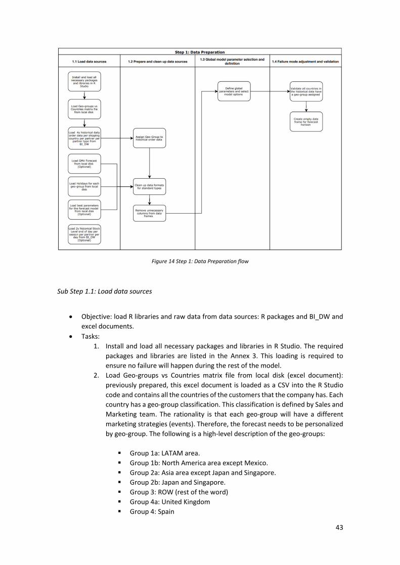
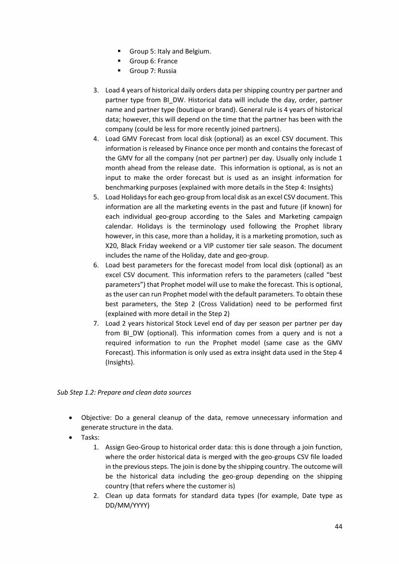
Sub Step 1.1: Load data sources .................................................................................................................... 43 Sub Step 1.2: Prepare and clean data sources ............................................................................................... 44 Sub Step 1.3: Global model parameter selection and definition ................................................................... 45 Sub Step 1.4: Failure mode adjustment and validation ................................................................................. 45

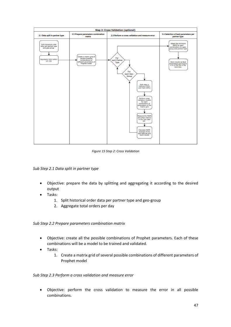
Step 2: Cross Validation ..................................................................................................................... 46 Sub Step 2.1 Data split in partner type .......................................................................................................... 47 Sub Step 2.2 Prepare parameters combination matrix ................................................................................. 47 Sub Step 2.3 Perform a cross validation and measure error ......................................................................... 47 Sub Step 2.4 Selection of best parameters per partner type ........................................................................ 48

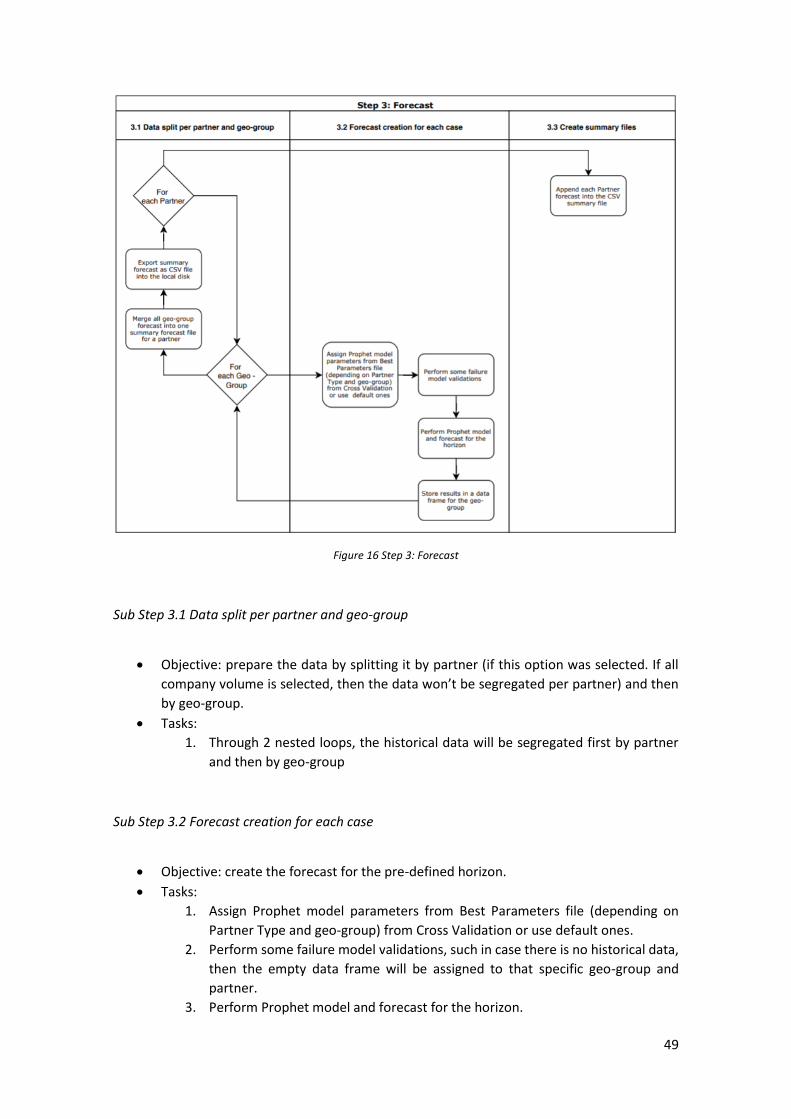
Step 3: Forecast ................................................................................................................................. 48 Sub Step 3.1 Data split per partner and geo-group ....................................................................................... 49 Sub Step 3.2 Forecast creation for each case ................................................................................................ 49 Sub Step 3.3 Create summary files ................................................................................................................ 50

Step 4: Insights ................................................................................................................................... 50

VI

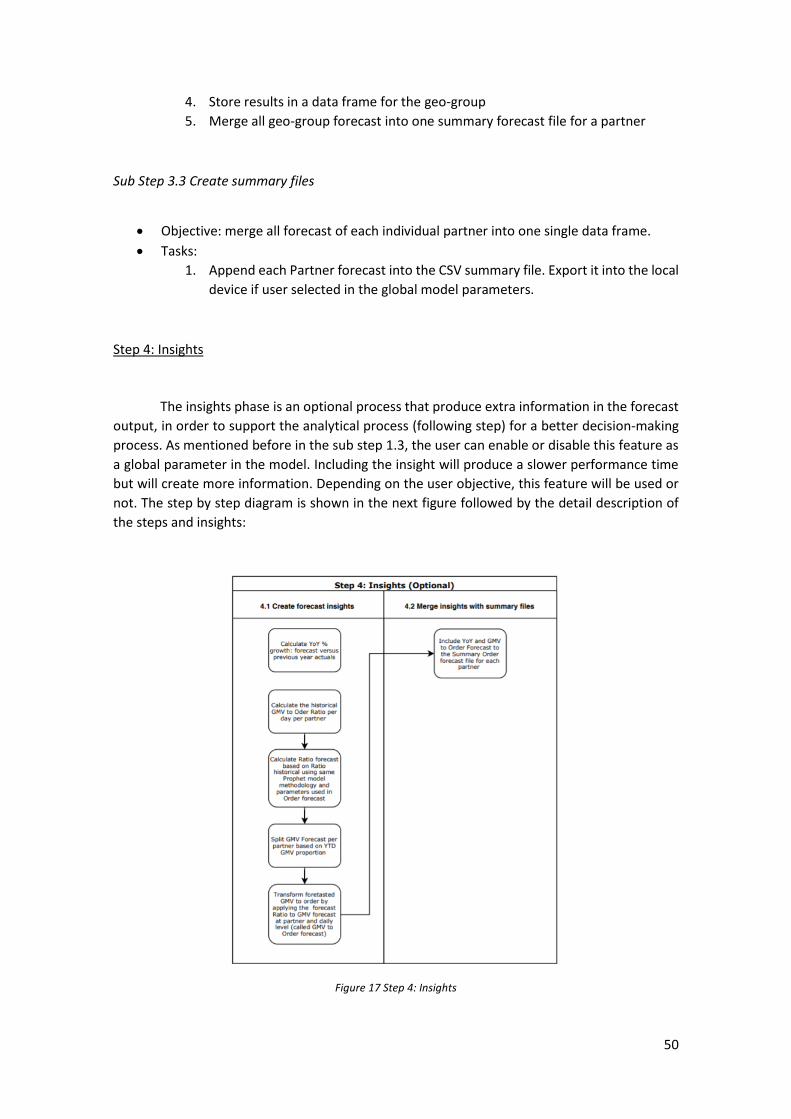
Sub Step 4.1 Create forecast insights ............................................................................................................ 51 Sub Step 4.2 Merge insights with summary files ........................................................................................... 51

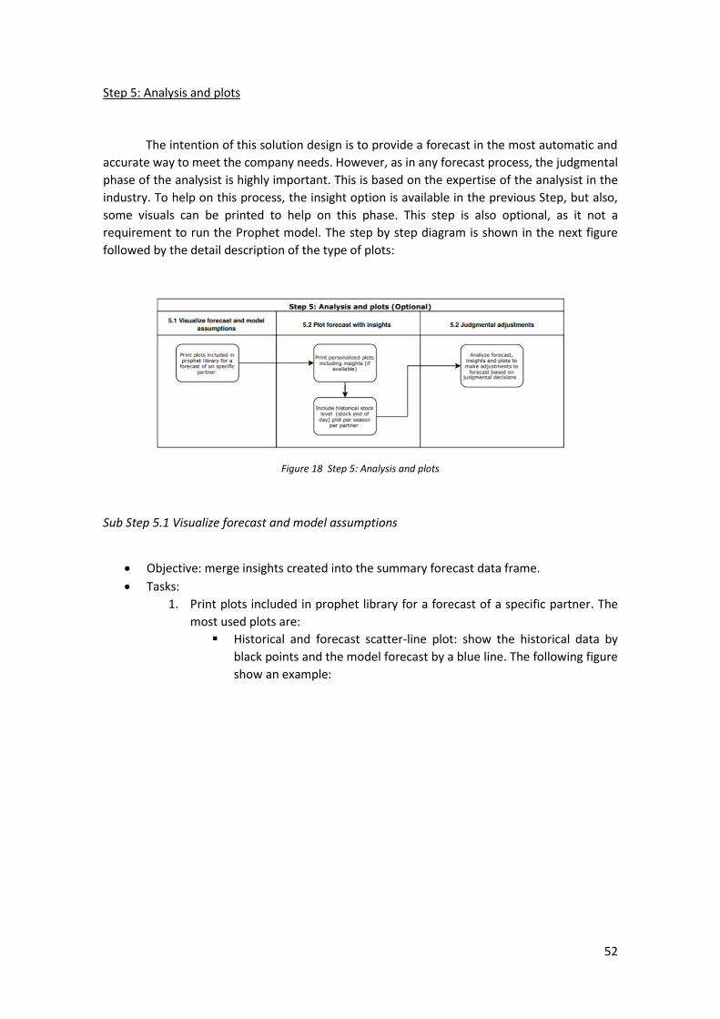
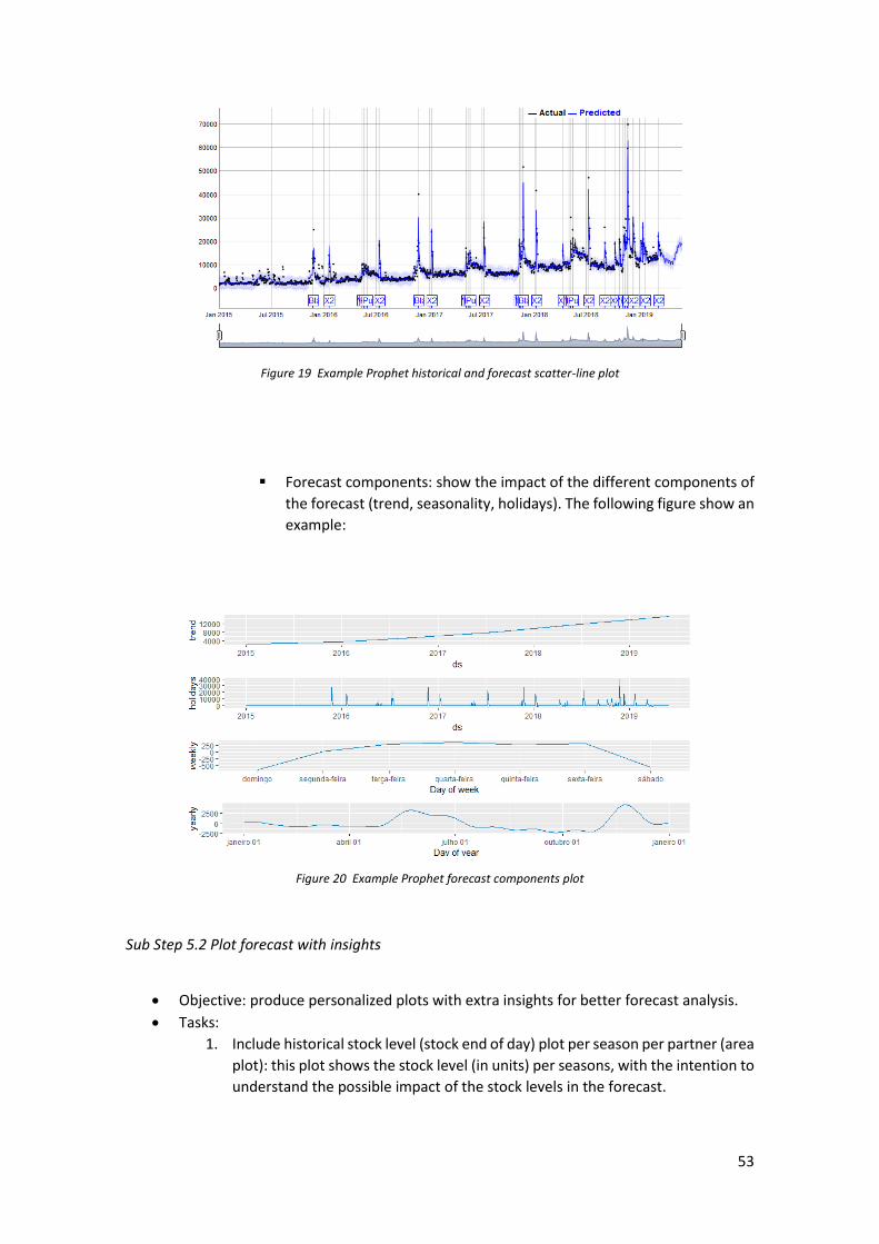
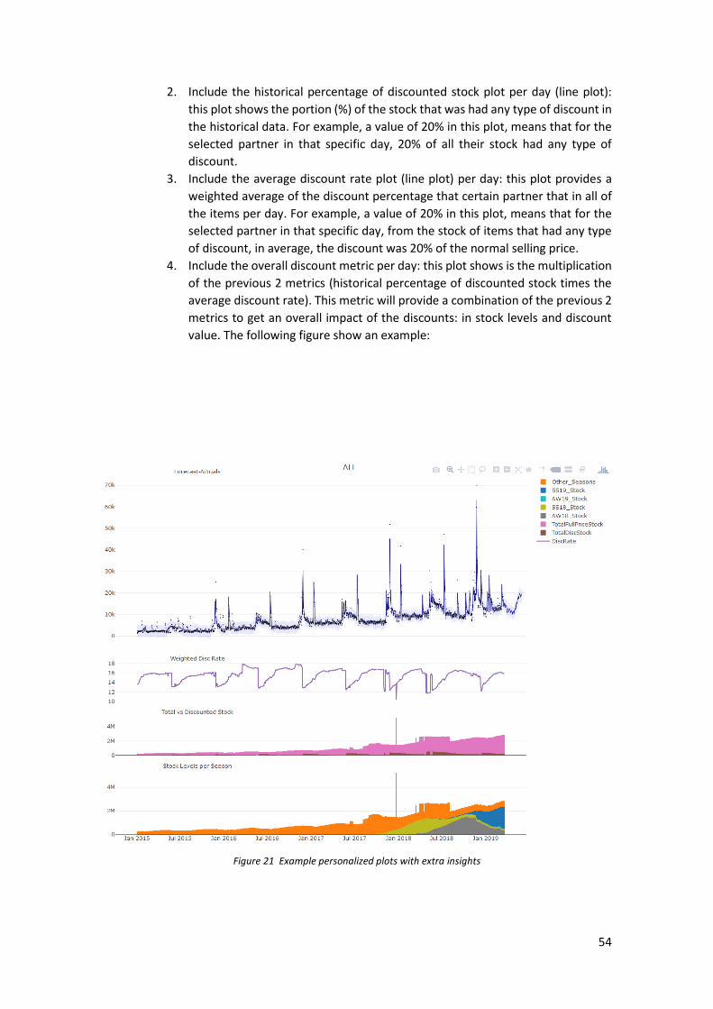
Step 5: Analysis and plots .................................................................................................................. 52 Sub Step 5.1 Visualize forecast and model assumptions ............................................................................... 52 Sub Step 5.2 Plot forecast with insights ........................................................................................................ 53 Sub Step 5.2 Judgmental adjustments ........................................................................................................... 55

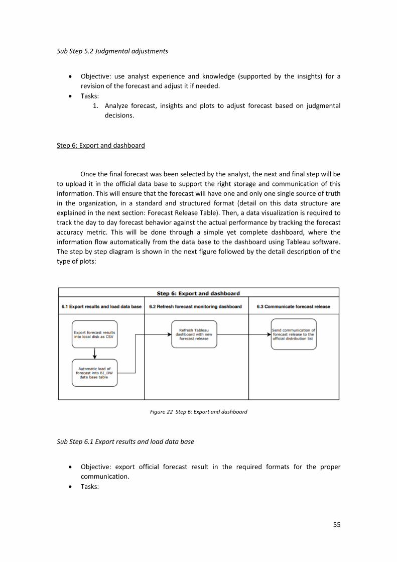
Step 6: Export and dashboard ............................................................................................................ 55 Sub Step 6.1 Export results and load data base ............................................................................................. 55 Sub Step 6.2 Refresh forecast monitoring dashboard ................................................................................... 56 Sub Step 6.3 Communicate forecast release ................................................................................................. 56

FORECAST RELEASE TABLE ............................................................................................................................ 57 FORECAST ACCURACY AND DASHBOARD REPORTING ........................................................................................... 58

VII. RESULTS AND DISCUSSION ...................................................................................................... 61

VIII. CONCLUSIONS ......................................................................................................................... 66

IX. LIMITATIONS AND RECOMMENDATIONS FOR FUTURE WORKS ................................................... 68

X. BIBLIOGRAPHY ............................................................................................................................ 70

XI. ANNEXES ..................................................................................................................................... 73

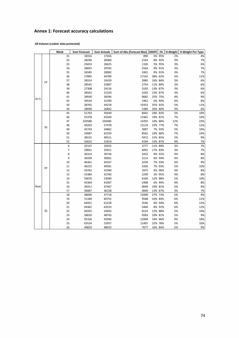
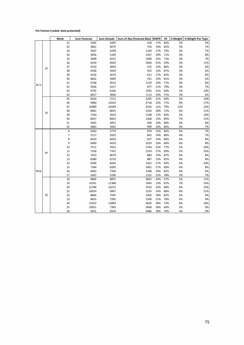
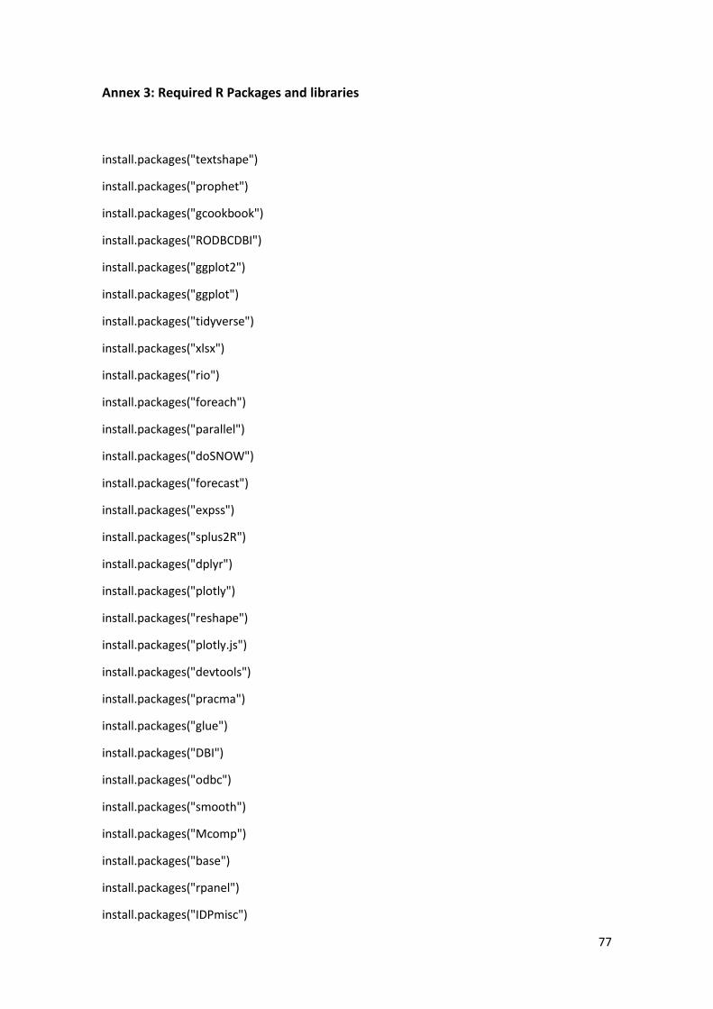
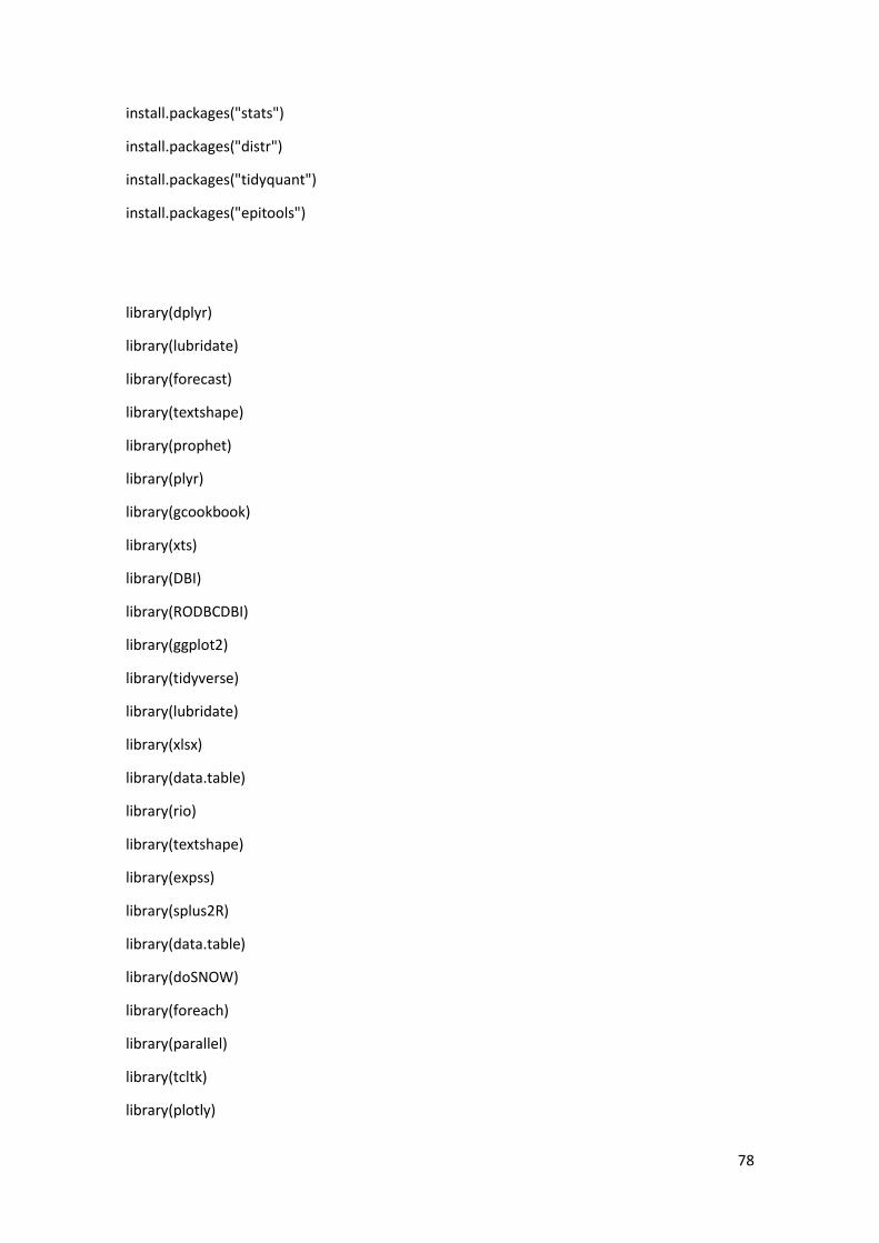
ANNEX 1: FORECAST ACCURACY CALCULATIONS ................................................................................................ 74 ANNEX 2: ROOT CAUSE PRIORITIZATION MATRIX (VOTING) .................................................................................. 76 ANNEX 3: REQUIRED R PACKAGES AND LIBRARIES ............................................................................................. 77

VII

LIST OF FIGURES

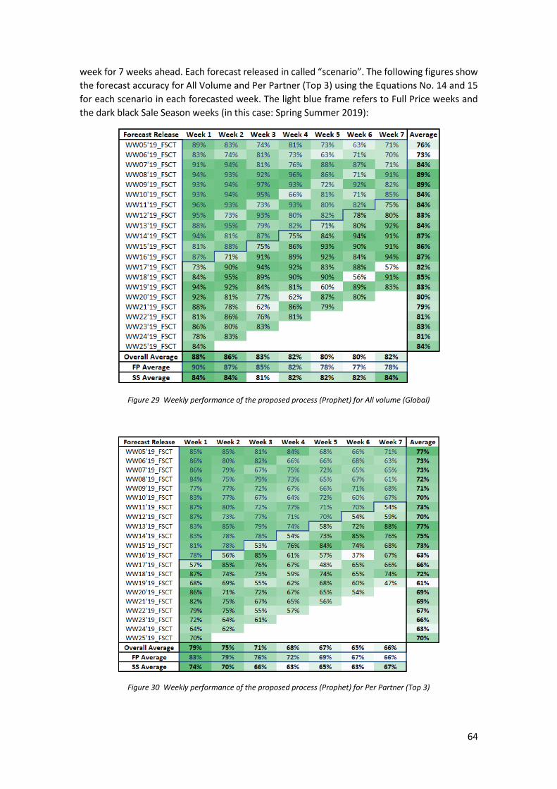
FIGURE 1 PROJECT GANT ROADMAP ..................................................................................................................... 8 FIGURE 2 GLOBAL OPERATION STRUCTURE........................................................................................................... 11 FIGURE 3 PROPHET ANALYST-IN-THE-LOOP FORECAST SCHEMATIC VIEW .................................................................... 16 FIGURE 4 EXAMPLE OF A MARKETING AND SALES CALENDAR ................................................................................... 26 FIGURE 5 FULL PRICE AS IS PROCESS ................................................................................................................... 28 FIGURE 6 SALE SEASON AS IS PROCESS ................................................................................................................ 31 FIGURE 7 ACTUAL FORECAST ACCURACY PERFORMANCE ALL VOLUME AND PER PARTNER LEVELS ................................... 33 FIGURE 8 BLACK FRIDAY WEEKEND MAPE PERFORMANCE ALL VOLUME SCENARIO DURING AW18 SALE SEASON .............. 34 FIGURE 9 BLACK FRIDAY WEEKEND PERFORMANCE TOP 3 BOUTIQUES SCENARIO DURING AW18 SALE SEASON .................. 35 FIGURE 10 CAUSE AND EFFECT DIAGRAM FOR THE PROBLEM STATEMENT AND PRIORITIZATION RESULTS ........................... 37 FIGURE 11 SOLUTION SOFTWARE STRUCTURE DESIGN ............................................................................................. 40 FIGURE 12 OVERVIEW OF THE SOLUTION STEPS ..................................................................................................... 41 FIGURE 13 SOLUTION FORECAST RELEASE SCHEMA ................................................................................................. 41 FIGURE 14 STEP 1: DATA PREPARATION FLOW ...................................................................................................... 43 FIGURE 15 STEP 2: CROSS VALIDATION ............................................................................................................... 47 FIGURE 16 STEP 3: FORECAST ............................................................................................................................ 49 FIGURE 17 STEP 4: INSIGHTS ............................................................................................................................. 50 FIGURE 18 STEP 5: ANALYSIS AND PLOTS ............................................................................................................ 52 FIGURE 19 EXAMPLE PROPHET HISTORICAL AND FORECAST SCATTER-LINE PLOT ........................................................... 53 FIGURE 20 EXAMPLE PROPHET FORECAST COMPONENTS PLOT ................................................................................. 53 FIGURE 21 EXAMPLE PERSONALIZED PLOTS WITH EXTRA INSIGHTS ............................................................................ 54 FIGURE 22 STEP 6: EXPORT AND DASHBOARD ...................................................................................................... 55 FIGURE 23 EXAMPLE OF A STANDARD FORECAST RELEASE COMMUTATION E-MAIL ....................................................... 57 FIGURE 24 TABLEAU JOIN TABLES DESIGN FOR FORECAST DASHBOARD ....................................................................... 58 FIGURE 25 EXAMPLE FINAL FORECAST DASHBOARD ............................................................................................... 58 FIGURE 26 EXAMPLE FINAL FORECAST DASHBOARD (DATA PROTECTED) ..................................................................... 59 FIGURE 27 FORECAST ACCURACY COMPARISONS AS IS PROCESS WITH NEW (PROPHET) ............................................... 62 FIGURE 28 DAILY FORECAST ACCURACY PROPHET AND AUTO ARIMA ....................................................................... 63 FIGURE 29 WEEKLY PERFORMANCE OF THE PROPOSED PROCESS (PROPHET) FOR ALL VOLUME (GLOBAL) ......................... 64 FIGURE 30 WEEKLY PERFORMANCE OF THE PROPOSED PROCESS (PROPHET) FOR PER PARTNER (TOP 3) .......................... 64

VIII

LIST OF TABLES

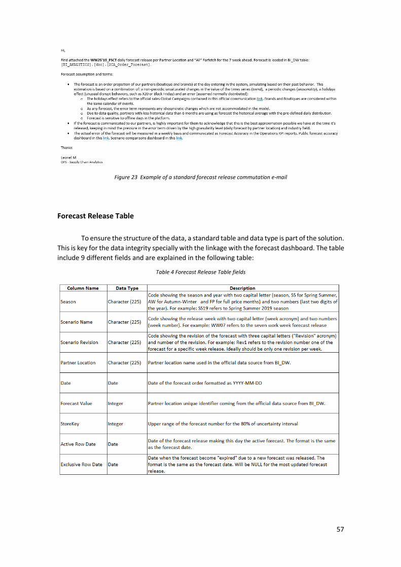
TABLE 1 PROPHET PARAMETERS SUMMARY (WITH R DOCUMENTATION DEFINITION) ..................................................... 20 TABLE 2 WEIGHTED AVERAGE FORECAST ACCURACY FULL PRICE, SALE SEASON AND OVERALL FOR AS IS PROCESS .............. 33 TABLE 3 AW18 FORECAST RELEASES WITH ADJUSTMENTS ....................................................................................... 34 TABLE 4 FORECAST RELEASE TABLE FIELDS ............................................................................................................ 57 TABLE 5 WEEKS AVAILABLE FOR FORECAST ACCURACY COMPARISONS ...................................................................... 62

IX

LIST OF EQUATIONS

EQUATION 1 BAYESIAN EQUATION ..................................................................................................................... 15 EQUATION 2 ADDITIVE DECOMPOSITION MODEL .................................................................................................... 16 EQUATION 3 MULTIPLICATIVE DECOMPOSITION MODEL .......................................................................................... 16 EQUATION 4 BASIC STRUCTURAL TIME SERIES EQUATION ........................................................................................ 17 EQUATION 5 PIECEWISE LOGISTIC GROWTH FOR NON-LINEAR TREND ......................................................................... 17 EQUATION 6 PIECEWISE LINEAR GROWTH FOR LINEAR TREND ................................................................................... 17 EQUATION 7 ADJUSTMENT OF CHANGEPOINTS ...................................................................................................... 18 EQUATION 8 SEASONAL APPROXIMATION ............................................................................................................ 18 EQUATION 9 SEASONAL GENERATIVE APPROXIMATION WITH PRIOR PARAMETER .......................................................... 19 EQUATION 10 MATRIX OF HOLIDAYS REGRESSORS ................................................................................................. 19 EQUATION 11 HOLIDAYS PROPHET COMPONENT ................................................................................................... 19 EQUATION 12 BASIC MEAN ABSOLUTE PERCENTAGE ERROR ................................................................................... 21 EQUATION 13 FORECAST ACCURACY METRIC ....................................................................................................... 21 EQUATION 14 FORECAST ACCURACY METRIC FOR ALL VOLUME................................................................................ 21 EQUATION 15 FORECAST ACCURACY METRIC PER PARTNER ..................................................................................... 21

.

X

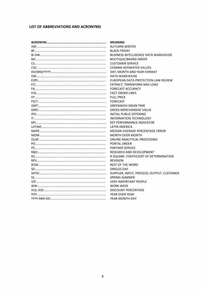
LIST OF ABBREVIATIONS AND ACRONYMS

ACRONYM………………………………………………………………. MEANING AW……………………………………………………………………………. AUTUMN-WINTER BF……………………………………………………………………………… BLACK FRIDAY BI DW……………………………………………………………………….. BUSINESS INTELLIGENCE DATA WAREHOUSE BO…………………………………………………………………………….. BOUTIQUE/BRAND ORDER CS……………………………………………………………………………… CUSTOMER SERVICE CSV…………………………………………………………………………… COMMA-SEPARATED VALUES DD/MM/YYYY……………………………………………………………. DAY, MONTH AND YEAR FORMAT DW……………………………………………………………………………. DATA WAREHOUSE EDPL…………………………………………………………………………. EUROPEAN DATA PROTECTION LAW REVIEW ETL……………………………………………………………………………. EXTRACT, TRANSFORM AND LOAD FA……………………………………………………………………………… FORECAST ACCURACY FOL……………………………………………………………………………. FACT ORDER LINES FP……………………………………………………………………………… FULL PRICE FSCT………………………………………………………………………….. FORECAST GMT………………………………………………………………………….. GREENWICH MEAN TIME GMV…………………………………………………………………………. GROSS MERCHANDISE VALUE IPO……………………………………………………………………………. INITIAL PUBLIC OFFERING IT………………………………………………………………………………. INFORMATION TECHNOLOGY KPI…………………………………………………………………………….. KEY PERFORMANCE INDICATOR LATAM………………………………………………………………………. LATIN AMERICA MAPE…………………………………..…………………………………… MEDIAN AVERAGE PERCENTAGE ERROR MOM………………………………………………………………………… MONTH OVER MONTH OLAP…………………………………………………………………………. ONLINE ANALYTICAL PROCESSING PO…………………………………………………………………………….. PORTAL ORDER PS……………………………………………………………………………… PARTNER SERVICE R&D………………………………………………………………………….. RESEARCH AND DEVELOPMENT R2……………………………………………………………………………… R SQUARE: COEFFICIENT OF DETERMINATION REV…………………………………………………………………………… REVISION ROW…………………………………………………………………………. REST OF THE WORD SD…………………………………………………………………………….. SINGLES DAY SIPOC………………………………………………………………………… SUPPLIER, INPUT, PROCESS, OUTPUT, CUSTOMER SS……………………………………………………………………………… SPRING-SUMMER VIP……………………………………………………………………………. VERY IMPORTANT PEOPLE WW………………………………………………………………………….. WORK WEEK X10, X20……………………………………………………………………. DISCOUNT PERCENTAGE YOY…………………………………………………………………………… YEAR OVER YEAR YYYY-MM-DD………………………………............................... YEAR-MONTH-DAY

I. Introduction

2

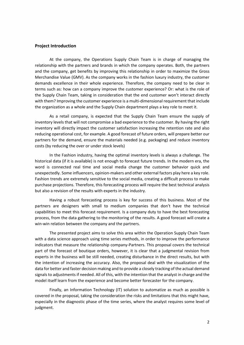
Project Introduction

At the company, the Operations Supply Chain Team is in charge of managing the

relationship with the partners and brands in which the company operates. Both, the partners

and the company, get benefits by improving this relationship in order to maximize the Gross

Merchandise Value (GMV). As the company works in the fashion luxury industry, the customer

demands excellence in their whole experience. Therefore, the company need to be clear in

terms such as: how can a company improve the customer experience? Or: what is the role of

the Supply Chain Team, taking in consideration that the end customer won’t interact directly

with them? Improving the customer experience is a multi-dimensional requirement that include

the organization as a whole and the Supply Chain department plays a key role to meet it.

As a retail company, is expected that the Supply Chain Team ensure the supply of

inventory levels that will not compromise a bad experience to the customer. By having the right

inventory will directly impact the customer satisfaction increasing the retention rate and also

reducing operational cost, for example. A good forecast of future orders, will prepare better our

partners for the demand, ensure the materials needed (e.g. packaging) and reduce inventory

costs (by reducing the over or under stock levels)

In the Fashion industry, having the optimal inventory levels is always a challenge. The

historical data (if it is available) is not enough to forecast future trends. In the modern era, the

word is connected real time and social media change the customer behavior quick and

unexpectedly. Some influencers, opinion-makers and other external factors play here a key role.

Fashion trends are extremely sensitive to the social media, creating a difficult process to make

purchase projections. Therefore, this forecasting process will require the best technical analysis

but also a revision of the results with experts in the industry.

Having a robust forecasting process is key for success of this business. Most of the

partners are designers with small to medium companies that don’t have the technical

capabilities to meet this forecast requirement. Is a company duty to have the best forecasting

process, from the data gathering to the monitoring of the results. A good forecast will create a

win-win relation between the company and the partners.

The presented project aims to solve this area within the Operation Supply Chain Team

with a data science approach using time series methods, in order to improve the performance

indicators that measure the relationship company-Partners. This proposal covers the technical

part of the forecast of boutique orders, however, it is clear that a judgmental revision from

experts in the business will be still needed, creating disturbance in the direct results, but with

the intention of increasing the accuracy. Also, the proposal deal with the visualization of the

data for better and faster decision making and to provide a closely tracking of the actual demand

signals to adjustments if needed. All of this, with the intention that the analyst in charge and the

model itself learn from the experience and become better forecaster for the company.

Finally, an Information Technology (IT) solution to automatize as much as possible is

covered in the proposal, taking the consideration the risks and limitations that this might have,

especially in the diagnostic phase of the time series, where the analyst requires some level of

judgment.

3

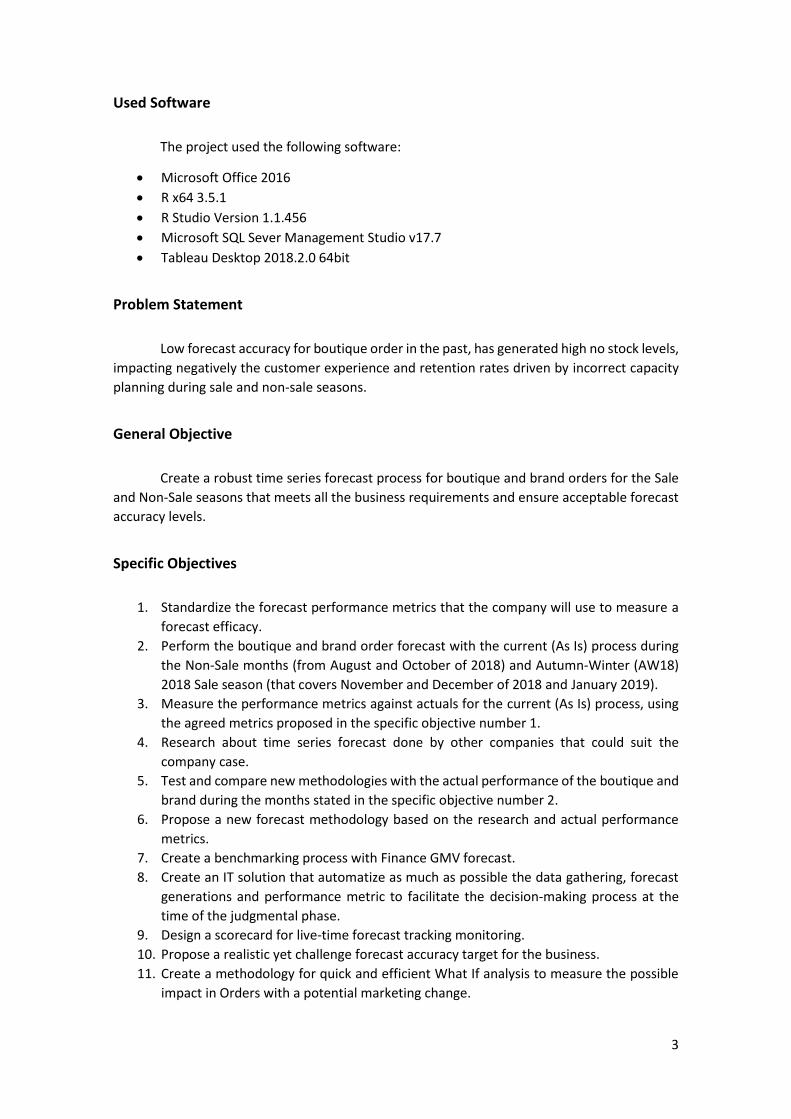
Used Software

The project used the following software:

• Microsoft Office 2016

• R x64 3.5.1

• R Studio Version 1.1.456

• Microsoft SQL Sever Management Studio v17.7

• Tableau Desktop 2018.2.0 64bit

Problem Statement

Low forecast accuracy for boutique order in the past, has generated high no stock levels,

impacting negatively the customer experience and retention rates driven by incorrect capacity

planning during sale and non-sale seasons.

General Objective

Create a robust time series forecast process for boutique and brand orders for the Sale

and Non-Sale seasons that meets all the business requirements and ensure acceptable forecast

accuracy levels.

Specific Objectives

1. Standardize the forecast performance metrics that the company will use to measure a

forecast efficacy.

2. Perform the boutique and brand order forecast with the current (As Is) process during

the Non-Sale months (from August and October of 2018) and Autumn-Winter (AW18)

2018 Sale season (that covers November and December of 2018 and January 2019).

3. Measure the performance metrics against actuals for the current (As Is) process, using

the agreed metrics proposed in the specific objective number 1.

4. Research about time series forecast done by other companies that could suit the

company case.

5. Test and compare new methodologies with the actual performance of the boutique and

brand during the months stated in the specific objective number 2.

6. Propose a new forecast methodology based on the research and actual performance

metrics.

7. Create a benchmarking process with Finance GMV forecast.

8. Create an IT solution that automatize as much as possible the data gathering, forecast

generations and performance metric to facilitate the decision-making process at the

time of the judgmental phase.

9. Design a scorecard for live-time forecast tracking monitoring.

10. Propose a realistic yet challenge forecast accuracy target for the business.

11. Create a methodology for quick and efficient What If analysis to measure the possible

impact in Orders with a potential marketing change.

4

Scope and Limitations

The scope of the project covers the boutique and brand forecast at orders level in the

required granularity.

The limitations of the project are the following:

• Historical data available: some boutiques and brands could be recently joined the

company, therefore there might not be enough historical data to perform a trustful

forecast

• Sales and marketing calendar strategies:

o Boutique Order forecast is aligned to the calendar, however, last minute

changes in the strategy will affect the forecast.

o Brand forecast is also aligned to the calendar, however, brands have the

freedom to decide their own calendar that might or not be shared with the

company. Therefore, is expected that brand order forecast might suffer a lower

forecast accuracy due to this limitation.

o Since the calendar is released for many other departments that require a very

level of detail, in the case of order forecast and for both cases (boutiques and

brands) not all levels of granularity of the calendar are included as an input in

the forecasting model (e.g. Customer Tier).

• Data privacy: due to the European Data Protection Law Review (EDPL) and Initial public

offering (IPO) regulations, some of the data used in this report might be protected or

hidden. The actual and forecast data has been protected by multiplying it by a constant.

As the results and mainly shown in percentages, this won´t scarify any quality of the

report. The company and partners names have been protected as well by naming then

as “company” and “boutique n”, where n can be 1,2, …, n.

Business Requirements

The order forecast needs to meet the following business requirements:

• Granularity: overall and by boutique (or brand) and by day GMT.

• Boutique and brand to be included in the forecast:

o Must include all partners of the company.

• The forecasts need to be easily adjustable for last minute changes in the Sale and

Marketing calendar.

• The reporting of the forecast need to include all the agreed daily KPI (Key Performance

Indicator) and have two approaches:

o Daily forecast performance: includes the Overall and by boutique (and brand)

forecast performance.

o Weekly forecast performance: aggregated per week KPIs measurements

grouped by Store Tier, not by individual boutique/brand levels.

• The selected forecasts, must be stored in a single version of the truth that can be easily

shared with other departments.

5

• The overall forecast process must be as automated as possible without sacrificing

accuracy, including the ETL process from the data warehouse, data analytics and data

visualization.

Justification: business case and importance

The importance to have a high-quality forecast of boutique and brand orders in Supply

Chain department is key for the success of the company and the company’s partners. The

following list explain the key justification points of the project:

• Partners capacity planning: the partners need an accurate forecast of orders to prepare

their human resources to high and low volume seasons. This is key to increase their

performance supplying the orders on time and high quality. A low-quality forecast, could

create over or under capacity resources, putting in danger the sales expectations for the

partner and the company itself.

• Service center capacity planning: the order forecast is used by the company to plan the

capacity of the service center department. This department is in charge to answer any

query by customers and/or partners. A low-quality forecast could impact their KPIs that

measure the speed of answer and solve a problem to their customers. The image of the

company could be impacted as well, if there is not enough resources available to satisfy

the customer’s needs.

• Finance expectations: the partners use the order forecast to calculate their profit at the

end of a period. This forecast justifies the partnership with the company, as it creates a

overview of the future sales. For each sale, one portion of it, goes to the partner and

another to the company. In order to justify the rentability of this partnership, the

partners need to ensure enough amount of orders to cover their fixed cost. Therefore,

this forecast is highly sensitive to the relationship with the company and the partners.

• Carriers capacity planning: considered as a third-party partner, the carrier is highly

important to the success of the order fulfillment. The carrier needs to prepare their

capacity to ensure the right delivery of the order to their destination. The carrier uses

the order forecast to plan their capacity and justify their rentability.

• Packaging planning: the company is the one paying for the packaging of the orders.

Having the right estimation of boxes to pack the order is key in the process. If the

amount of orders is right, but not the number of boxes, the whole process would be

impacted and the customer will suffer a delay. The Supply Chain department, is the one

in charge of ensure this packaging capacity, by analyzing the order forecast.

II. Methodology

7

Project Methodology and Roadmap

The project will be structured in a theoretical-practical way to ensure success in the

results. In general terms, will follow the ongoing process of the scientific method:

• Observation: understand the As Is process and business acumen. Perform the

current forecasting processes and deliver them to the customer without

affecting the business. Measure current performance with As Is procedure.

• Research and Development (R&D): investigate in the time series-forecasting

field, potential solutions that can solve the problem statement.

• Hypothesis: select a potential solution with null hypothesis that will increase the

accuracy and meet the business requirements

• Experiment: perform coding in R Studio with potential solutions and test the

results.

o If experiment does not work, go back to experiment by performing the

required code improvement and troubleshooting.

• Analyze data and draw conclusions: understand if the experiment had positive

results and meets all the business requirements in order to make a final

recommendation.

• Project and change management: perform typical project and change

management tasks to go live with the solution

• Continuous improvement: ensure ongoing improvements for the future.

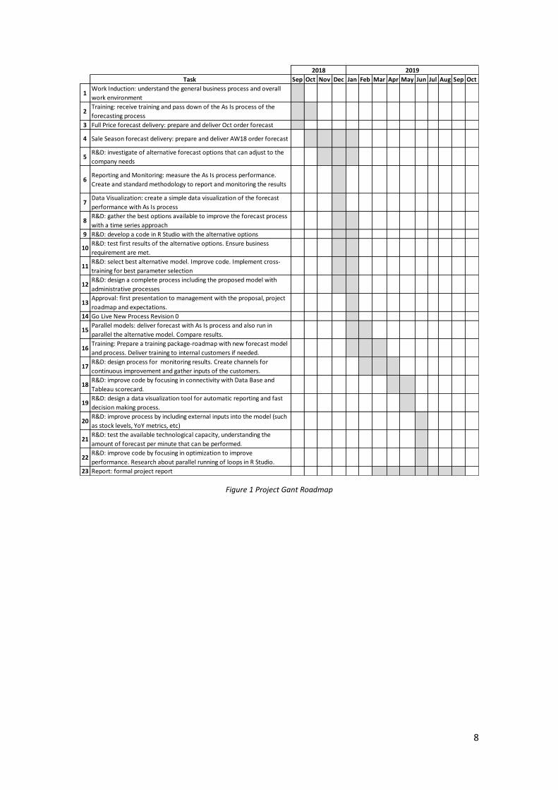
Based on the project management task, the following figure show the proposed project

Gantt, showing with more details the required actions and approximate timing to have them

completed. Since this project is not an independent task from the business as usual, some

parallel activities will take place in the experiment phase. This is required since the business can

not wait for the solution to be implement (order forecast is a critical activity).

8

Figure 1 Project Gant Roadmap

Task Sep Oct Nov Dec Jan Feb Mar Apr May Jun Jul Aug Sep Oct

1Work Induction: understand the general business process and overall

work environment

2Training: receive training and pass down of the As Is process of the

forecasting process

3 Full Price forecast delivery: prepare and deliver Oct order forecast

4 Sale Season forecast delivery: prepare and deliver AW18 order forecast

5R&D: investigate of alternative forecast options that can adjust to the

company needs

6Reporting and Monitoring: measure the As Is process performance.

Create and standard methodology to report and monitoring the results

7Data Visualization: create a simple data visualization of the forecast

performance with As Is process

8R&D: gather the best options available to improve the forecast process

with a time series approach

9 R&D: develop a code in R Studio with the alternative options

10R&D: test first results of the alternative options. Ensure business

requirement are met.

11R&D: select best alternative model. Improve code. Implement cross-

training for best parameter selection

12R&D: design a complete process including the proposed model with

administrative processes

13Approval: first presentation to management with the proposal, project

roadmap and expectations.

14 Go Live New Process Revision 0

15Parallel models: deliver forecast with As Is process and also run in

parallel the alternative model. Compare results.

16Training: Prepare a training package-roadmap with new forecast model

and process. Deliver training to internal customers if needed.

17R&D: design process for monitoring results. Create channels for

continuous improvement and gather inputs of the customers.

18R&D: improve code by focusing in connectivity with Data Base and

Tableau scorecard.

19R&D: design a data visualization tool for automatic reporting and fast

decision making process.

20R&D: improve process by including external inputs into the model (such

as stock levels, YoY metrics, etc)

21R&D: test the available technological capacity, understanding the

amount of forecast per minute that can be performed.

22R&D: improve code by focusing in optimization to improve

performance. Research about parallel running of loops in R Studio.

23 Report: formal project report

2018 2019

III. Company History

10

Founded by J. Neves in 2008, the company is an online luxury fashion marketplace,

which connects more than 1200 partners - luxury boutiques, brands and warehouses - to

millions of customers all over the world, on a single website. 11 years after its launch, the

company has partners in 49 countries, and has clients in more than 190 countries. It has offices

in 13 different cities and is growing over 50% every year, having generated a record Gross

Merchandise Value (GMV) in 2018 (Halliday, 2019), being since 2017 the first Portuguese

company valued more than 1 billion dollars. In October 2018, the firm entered the New York

stock exchange and in the same year, revenue rose by 56% and the number of placed orders

increased 58%. The company also owns two British renowned boutiques and an American

footwear brand.

In 2019 the company already announced the acquisition of JD.com's luxury platform

Toplife to enable the gateway to the China market and the partnership with Harrods, to create

and manage the department's e-commerce platform (Suen, 2019).

The company’s aim is to offer the luxury goods customers a unique, creative, excellence

service. The company's business model is what distinguishes it from its competitors and is the

one of a marketplace: it does not hold any stock or have its own transportation system. The

partners, who, due to their presence on the website, have a visibility and accessibility they would

not have otherwise, sell directly from their own stock points to the clients. The client only knows

which partner he/she is buying from at the time of delivery, as all the information flow passes

through and is managed by the company. In order to guarantee the desired service levels, the

company controls the whole process, from content creation through delivery to the client's

house to the post-sales customer service. The delivery service is outsourced from third-party

logistics partners (3PL), which charge to the company a shipping fee. The price payed by the

customers includes the item's price, the company’s margin and the shipping fee.

The business model is, however, associated with higher complexity and numerous

challenges, such as the risk of stock out, the dependency on the partner's performance, and the

complexity of delivery (as there are a great number of possible routes).

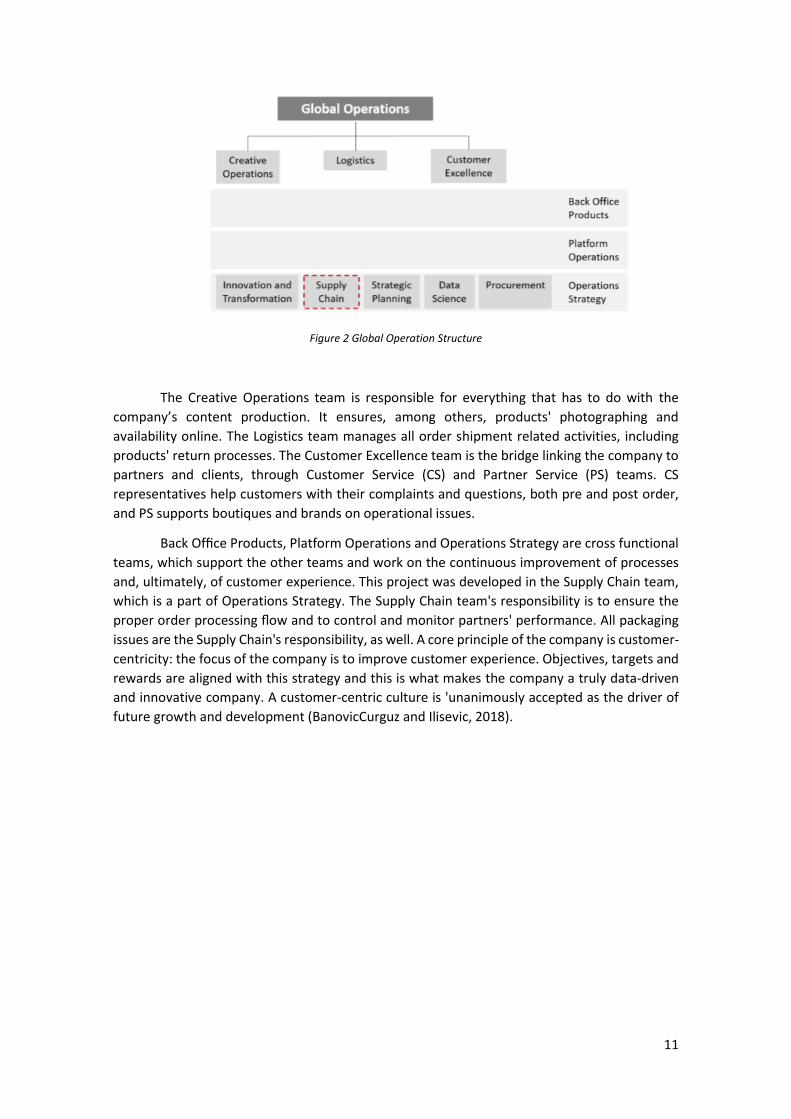
The company is organized in the following departments: Global Operations, Product,

Communications, Technology, Finance, Strategy and Commercial. The Global Operations

Department is responsible for all activities related with daily ecommerce and consists of several

teams, as shown in the following figure:

11

Figure 2 Global Operation Structure

The Creative Operations team is responsible for everything that has to do with the

company’s content production. It ensures, among others, products' photographing and

availability online. The Logistics team manages all order shipment related activities, including

products' return processes. The Customer Excellence team is the bridge linking the company to

partners and clients, through Customer Service (CS) and Partner Service (PS) teams. CS

representatives help customers with their complaints and questions, both pre and post order,

and PS supports boutiques and brands on operational issues.

Back Office Products, Platform Operations and Operations Strategy are cross functional

teams, which support the other teams and work on the continuous improvement of processes

and, ultimately, of customer experience. This project was developed in the Supply Chain team,

which is a part of Operations Strategy. The Supply Chain team's responsibility is to ensure the

proper order processing flow and to control and monitor partners' performance. All packaging

issues are the Supply Chain's responsibility, as well. A core principle of the company is customer-

centricity: the focus of the company is to improve customer experience. Objectives, targets and

rewards are aligned with this strategy and this is what makes the company a truly data-driven

and innovative company. A customer-centric culture is 'unanimously accepted as the driver of

future growth and development (BanovicCurguz and Ilisevic, 2018).

IV. Literature Review

13

General Time Series Forecasting in Fashion Industry

Creating an accurate forecast of any type of data is being researched and developed for

a long time in human history. Nowadays, is more crucial than in any other time in history due to

the current challenges the industry is facing. Several methods have been released that might or

might not suit best of a type of industry, all of them using the common data source: time series,

which consists of a set of observations ordered in time, on a given phenomenon (target variable).

Usually the measurements are equally spaced, e.g. by year, quarter, month, week, day. The most

important property of a time series is that the ordered observations are dependent through

time, and the nature of this dependence is of interest. (Dagum, 2010). As time is key component

in the data source, it adds another layer of complexity versus other common data sources in the

predicting machine learning processes.

In the present project, the industry of interest for the forecast process is the fashion

retail one. This raise even more challenges to the project objectives. The main challenge is the

type of data, as it depends of the stock availability. Amazon is a company leader in this type of

forecast and is consent of this extra roadblock. In their paper: “Probabilistic Demand Forecasting

at Scale” (Bose, Flunkert, Gasthaus, Januschowski, Lange, Salinas, Schelter, Seeger & Wang,

2017), the author refers that the demand forecasting problem constitutes in predicting the

demand for a group of items at a certain range of days in the future, given demand data for all

items up to the present, as well as other input data sources. In a retail context, demand in the

past typically refers to customer orders. Note that this is an approximation as demand is partially

unobserved: orders for an item are subject to the item’s availability. Therefore, forecasting

customer order will always have an extra error or assumption inherited in the data accuracy.

Currently, the fashion industry is characterized by a fierce competition that forces

companies to constantly change the range of products offered, vastly increasing the number of

collections. Traditionally, stylist design collections from six to eight months before the launch,

with a high risk due to demand volatility and short life cycle of fashion products (Arrigo, 2010).

At the same time, fashion industry demand is so difficult to forecast that companies which want

to keep up with the competition have already accepted that products need to be designed,

manufactured and delivered based on real-time demand (Christopher, 2004). Several authors

agree with the big challenge of forecasting this industry driven by the following summarized

characteristics (Christopher, 2004):

• Short life-cycles: the product is often ephemeral, designed to capture the mood of the

moment: consequently, the period in which it will be saleable is likely to be very short

and seasonal, measured in months or even weeks.

• High volatility: demand for these products is rarely stable or linear. It may be influenced

by the vagaries of weather, films, or even by pop stars and footballers.

• Low predictability: because of the volatility of demand it is extremely difficult to forecast

with any accuracy even total demand within a period, let alone week-by-week or item-

by-item demand.

• High impulse purchasing many buying decisions by consumers for these products are

made at the point of purchase. In other words, the shopper when confronted with the

product is stimulated to buy it, hence the critical need for “availability”.

14

These facts create that the historical data might not explain easily the future predictions,

due to external customer behavior factors. The importance of an accurate demand forecast is

vast in several sectors: finance, marketing, operations, supply chain among others. Demand

forecast is one of the most important inputs in capacity planning, especially in the fashion retail

industry. Poor forecasting effects are stock outs or high inventory, obsolescence, low service

level, rush orders, inefficient resource utilization and bullwhip propagating through the

upstream supply chain. As such, demand forecasting is a popular research topic and many

models for forecasting fashion products have been proposed in the literature over the past few

decades (Nenni, Giustiniano & Pirolo, 2013). In general terms, there are two types of forecast

methods (Hyndman, 2009):

• Quantitative forecasting can be applied when two conditions are satisfied: numerical

information about the past is available and it is reasonable to assume that some aspects

of the past patterns will continue. There is a wide range of quantitative forecasting

methods, often developed within specific disciplines for specific purposes.

• Qualitative forecasting methods are used when one or both above conditions does not

hold. They are also used to adjust quantitative forecasts, taking account of information

that was not able to be incorporated into the formal statistical model. These are not

purely guesswork—there are well-developed structured approaches to obtaining good

judgmental forecasts.

In the presented project, the selected method is a mix between quantitative and quality

types of forecast. The base of the forecast follows a quantitative type with a demand in scale

forecast with a decomposition – Bayesian approach. However, the is always a space dedicated

to the qualitative forecast, in the analytical part of the quantitative results, meaning that

judgmental criteria is also key in the forecast accuracy success.

Many literatures explain the methodology needed to perform a time series forecast,

however Hyndman (2009) proposes a simple basic steps to perform a forecast of any type, as

the following:

• Step 1: Problem definition: often this is most difficult part of forecasting. Defining the

problem carefully requires an understanding of how the forecasts will be used, who

requires the forecasts, and how the forecasting function fits within the organization

requiring the forecasts. A forecaster needs to spend time talking to everyone who will

be involved in collecting data, maintaining databases, and using the forecasts for future

planning.

• Step 2: Gathering information: there are always at least two kinds of information

required: statistical data and the accumulated expertise of the people who collect the

data and use the forecasts. Often, a difficulty will be obtaining enough historical data to

be able to fit a good statistical model. However, occasionally, very old data will not be

so useful due to changes in the system being forecast.

• Step 3: Preliminary (exploratory) analysis: always starting by graphing the data and

identify consistent patterns, trend, seasonality important, evidence of the presence of

business cycles, outliers in the data that need to be explained by those with expert

15

knowledge and how strong are the relationships among the variables available for

analysis.

• Step 4: Choosing and fitting models: which model to use depends on the availability of

historical data, the strength of relationships between the forecast variable and any

explanatory variables, and the way the forecasts are to be used. It is common to

compare two or three potential models.

• Step 5: Using and evaluating a forecasting model: once a model has been selected and

its parameters estimated, the model is to be used to make forecasts. The performance

of the model can only be properly evaluated after the data for the forecast period have

become available.

From the quantitative point of view, a Bayesian approach to inference from historical

data differs from the standard (frequentist) method for inference in its use of a prior distribution

to express the uncertainty present before seeing the data, and to allow the uncertainty

remaining after seeing the data to be expressed in the form of a posterior distribution (Hastie,

Tibshirani & Friedman, 2017). In general, the Bayesian equation is the following:

𝑃𝑟(𝜃|𝑍) = 𝑃𝑟(𝑍|𝜃) · 𝑃𝑟(𝜃)

∫ 𝑃𝑟(𝑍|𝜃) · 𝑃𝑟(𝜃)𝑑𝜃

Equation 1 Bayesian Equation

Where Pr(Z|θ) is the sampling model and Pr(θ) prior distribution for the parameters

reflecting the knowledge about θ before the study of the data.

On the other hand, the decomposition approach refers to the capacity of separate the

time series into a set of non-observable (latent) components that can be associated to different

types of temporal variations. The idea of time series decomposition is very old and was used for

the calculation of planetary orbits by seventeenth century astronomers (Dagum, 2010). Persons

(1919) was the first to state explicitly the assumptions of unobserved components in four basic

types of fluctuations (later, other authors will include others):

• A long-term tendency or secular trend.

• Cyclical movements super-imposed upon the long-term trend. These cycles appear to

reach their peaks during periods of industrial prosperity and their troughs during periods

of depressions, their rise and fall constituting the business-cycle.

• A seasonal movement within each year, the shape of which depends on the nature of

the series.

• Residual variations due to changes impacting individual variables or other major events

such as wars and national catastrophes affecting a number of variables.

Traditionally, the four variations have been assumed to be mutually independent from

one another and specified by means of an additive decomposition model:

16

𝑋𝑡 = 𝑇𝑡 + 𝐶𝑡 + 𝑆𝑡 + 𝐼𝑡

Equation 2 Additive decomposition model

Xt = Tt ∗ Ct ∗ St ∗ It

Equation 3 Multiplicative decomposition model

Where Xt denotes the observed series, Tt the long-term trend, Ct the business-cycle, St

seasonality and It the irregulars (also called as the error).

Prophet Model

In the presented project, the solution includes the usage of a Facebook open source

code for time series forecasting, called Prophet (Taylor & Letham, 2017), that was developed by

Sean J. Taylor with the collaboration of Benjamin Letham. In general terms, the methodology

has the following basic characteristics and approached:

• Is considered a forecasting “at scale” methodology: the structure of the code is robust

enough to handle different types of forecast data.

• Is a decomposition forecast type: the model uses a decomposition approach in several

regressors.

• Analysist-in-the loop approach: the authors consider that the judgmental-human

interaction is key in the forecast process, however, the model will create automated

forecast but include several visual tools for the analyst to make inspections is the most

critical cases.

Figure 3 Prophet Analyst-in-the-loop forecast schematic view

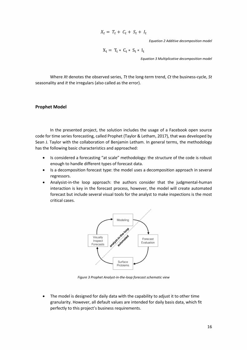
• The model is designed for daily data with the capability to adjust it to other time

granularity. However, all default values are intended for daily basis data, which fit

perfectly to this project’s business requirements.

17

Prophet use a decomposable time series model based on the structural time series

model proposed by A.C Harvey and S. Peters in their paper Estimation Procedures for Structural

Time Series Models (Harvel & Peters,1990) where “the essence of a structural model is that it is

formulated in terms of independent components which have a direct interpretation in terms of

quantities of interest. One of the most important models for economic time series is the basic

structural model: this consists of a trend, a seasonal and an irregular component:

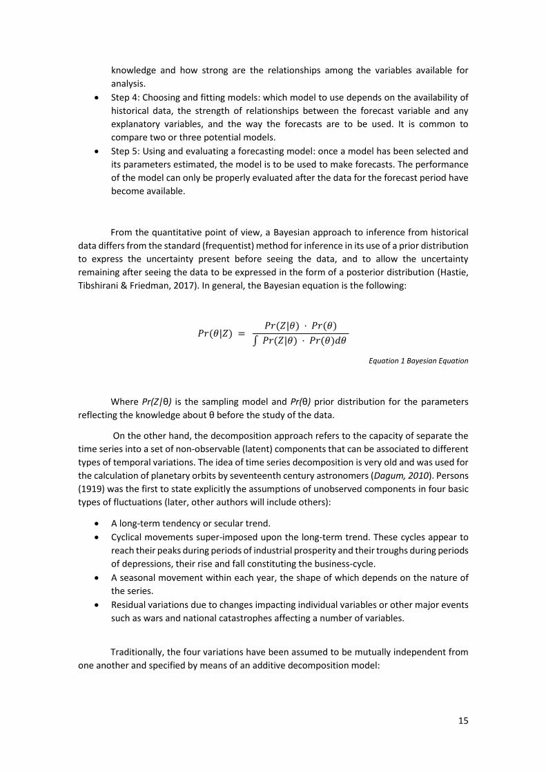
𝑦(𝑡) = 𝑔(𝑡) + 𝑠(𝑡) + ℎ𝑡 + 𝑒(𝑡)

Equation 4 Basic Structural Time Series equation

Where, g(t) is the trend function which models non-periodic changes in the value of the

time series, s(t) represents periodic changes and h(t) represent the effects of holidays which

occur on potentially irregular schedules over one o more days. The error term e(t) represent any

idiosyncratic changes which are not accommodated by the model (Taylor & Letham, 2017). The

following section provides an overview of each of these components (referenced directly for

Taylor and Letham paper) adding emphasis in the terms or parameters that were selected for

this project:

Prophet: The Trend

The library provides two types of trend: non-linear and liner trends. The main difference

from the theoretical point of view is if the demand being forecast can be considered unsaturated

or saturated. For saturated demand forecast, non-linear approach is used using a typical logistic

growth model. On the other hand, for unsaturated demand forecast, uses a simple linear

approach. For the presented project, the overall assumption is that the company is phasing a

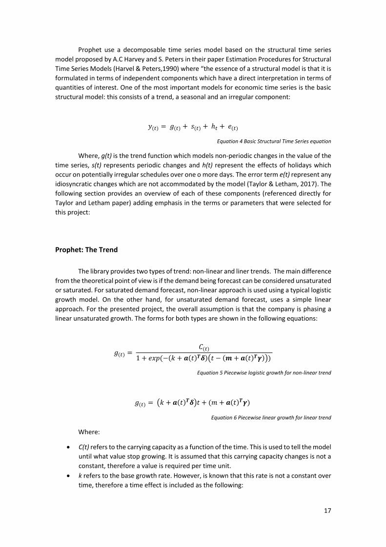
linear unsaturated growth. The forms for both types are shown in the following equations:

𝑔(𝑡) = 𝐶(𝑡)

1 + 𝑒𝑥𝑝(−(𝑘 + 𝒂(𝑡)𝑻𝜹)(𝑡 − (𝒎 + 𝒂(𝑡)𝑻𝜸)))

Equation 5 Piecewise logistic growth for non-linear trend

𝑔(𝑡) = (𝑘 + 𝒂(𝑡)𝑻𝜹)𝑡 + (𝑚 + 𝒂(𝑡)𝑻𝜸)

Equation 6 Piecewise linear growth for linear trend

Where:

• C(t) refers to the carrying capacity as a function of the time. This is used to tell the model

until what value stop growing. It is assumed that this carrying capacity changes is not a

constant, therefore a value is required per time unit.

• k refers to the base growth rate. However, is known that this rate is not a constant over

time, therefore a time effect is included as the following:

18

o k + a(t)t δ refers the growth rate at time t, which states as the base rate k plus

the trend changes in the historical data, defined with a vector δ containing all

the changepoints where the growth rate is allowed to change.

o Whether or not a changepoint is added to the growth rate is specified by the

vector a(t) Є {0, 1} where a value of 1 is assigned when t is higher or equal to the

changepoint and 0 otherwise.

o The amount and selection of changepoints can be added by the user as an input

vector in the model (vector δ). If not specified, potential changepoints are

selected automatically, given a set of candidates putting a sparse prior on δ ~

Laplace (0, τ). The parameter τ directly controls the flexibility of the model in

altering its rate. For the project, an automatic changepoint is preferred

specifying the parameter τ (called “changepoint.pior.scale”).

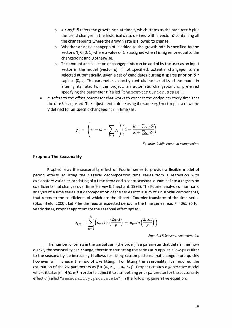
• m refers to the offset parameter that works to connect the endpoints every time that

the rate k is adjusted. The adjustment is done using the same a(t) vector plus a new one

𝛄 defined for an specific changepoint s in time j as:

𝜸𝑗 = (𝑠𝑗 − 𝑚 − ∑ 𝛾𝑙

𝑙<𝑗

) (1 − 𝑘 + ∑ 𝛿𝑙𝑙<𝑗

𝑘 + ∑ 𝛿𝑙𝑙≤𝑗)

Equation 7 Adjustment of changepoints

Prophet: The Seasonality

Prophet relay the seasonality effect on Fourier series to provide a flexible model of

period effects adjusting the classical decomposition time series from a regression with

explanatory variables consisting of a time trend and a set of seasonal dummies into a regression

coefficients that changes over time (Harvey & Shephard, 1993). The Fourier analysis or harmonic

analysis of a time series is a decomposition of the series into a sum of sinusoidal components,

that refers to the coefficients of which are the discrete Fournier transform of the time series

(Bloomfield, 2000). Let P be the regular expected period in the time series (e.g. P = 365.25 for

yearly data), Prophet approximate the seasonal effect s(t) as:

𝑆(𝑡) = ∑ (𝑎𝑛 𝑐𝑜𝑠 (2𝜋𝑛𝑡

𝑃) + 𝑏𝑛𝑠𝑖𝑛 (

2𝜋𝑛𝑡

𝑃) )

𝑁

𝑛=1

Equation 8 Seasonal Approximation

The number of terms in the partial sum (the order) is a parameter that determines how

quickly the seasonality can change, therefore truncating the series at N applies a low-pass filter

to the seasonality, so increasing N allows for fitting season patterns that change more quickly

however will increase the risk of overfitting. For fitting the seasonality, it’s required the

estimation of the 2N parameters as β = [a1, b1 , …, aN, bN ]T . Prophet creates a generative model

where it takes β ~ N (0, σ2) in order to adjust it to a smoothing prior parameter for the seasonality

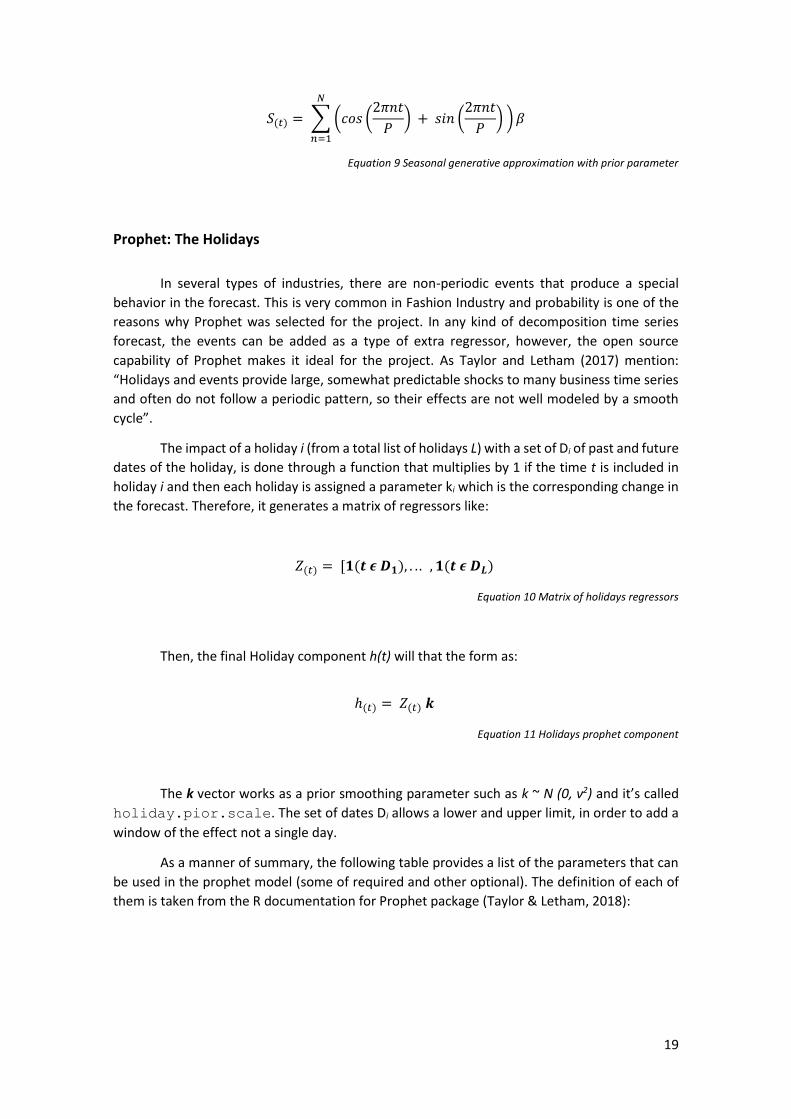
effect σ (called “seasonality.pior.scale”) in the following generative equation:

19

𝑆(𝑡) = ∑ (𝑐𝑜𝑠 (2𝜋𝑛𝑡

𝑃) + 𝑠𝑖𝑛 (

2𝜋𝑛𝑡

𝑃) ) 𝛽

𝑁

𝑛=1

Equation 9 Seasonal generative approximation with prior parameter

Prophet: The Holidays

In several types of industries, there are non-periodic events that produce a special

behavior in the forecast. This is very common in Fashion Industry and probability is one of the

reasons why Prophet was selected for the project. In any kind of decomposition time series

forecast, the events can be added as a type of extra regressor, however, the open source

capability of Prophet makes it ideal for the project. As Taylor and Letham (2017) mention:

“Holidays and events provide large, somewhat predictable shocks to many business time series

and often do not follow a periodic pattern, so their effects are not well modeled by a smooth

cycle”.

The impact of a holiday i (from a total list of holidays L) with a set of Di of past and future

dates of the holiday, is done through a function that multiplies by 1 if the time t is included in

holiday i and then each holiday is assigned a parameter ki which is the corresponding change in

the forecast. Therefore, it generates a matrix of regressors like:

𝑍(𝑡) = [𝟏(𝒕 𝝐 𝑫𝟏), . . . , 𝟏(𝒕 𝝐 𝑫𝑳)

Equation 10 Matrix of holidays regressors

Then, the final Holiday component h(t) will that the form as:

ℎ(𝑡) = 𝑍(𝑡) 𝒌

Equation 11 Holidays prophet component

The k vector works as a prior smoothing parameter such as k ~ N (0, ν2) and it’s called

holiday.pior.scale. The set of dates Di allows a lower and upper limit, in order to add a

window of the effect not a single day.

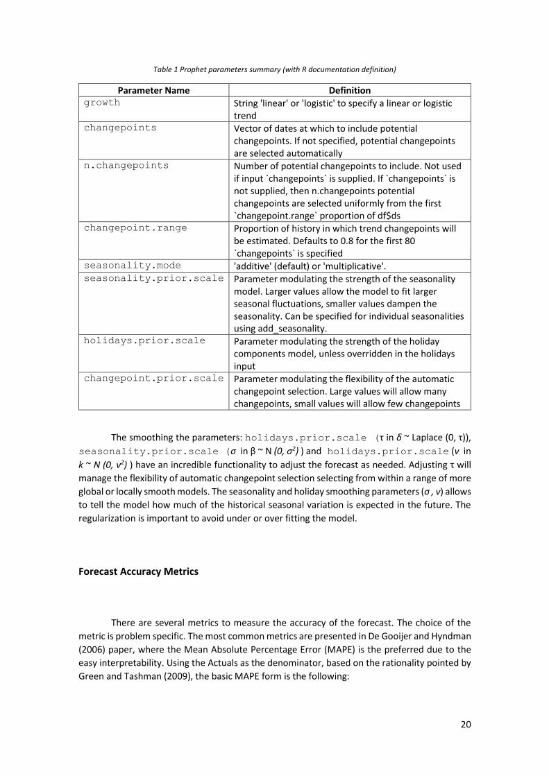
As a manner of summary, the following table provides a list of the parameters that can

be used in the prophet model (some of required and other optional). The definition of each of

them is taken from the R documentation for Prophet package (Taylor & Letham, 2018):

20

Table 1 Prophet parameters summary (with R documentation definition)

Parameter Name Definition growth String 'linear' or 'logistic' to specify a linear or logistic

trend changepoints Vector of dates at which to include potential

changepoints. If not specified, potential changepoints are selected automatically

n.changepoints Number of potential changepoints to include. Not used if input `changepoints` is supplied. If `changepoints` is not supplied, then n.changepoints potential changepoints are selected uniformly from the first `changepoint.range` proportion of df$ds

changepoint.range Proportion of history in which trend changepoints will be estimated. Defaults to 0.8 for the first 80 `changepoints` is specified

seasonality.mode 'additive' (default) or 'multiplicative'. seasonality.prior.scale Parameter modulating the strength of the seasonality

model. Larger values allow the model to fit larger seasonal fluctuations, smaller values dampen the seasonality. Can be specified for individual seasonalities using add_seasonality.

holidays.prior.scale Parameter modulating the strength of the holiday components model, unless overridden in the holidays input

changepoint.prior.scale Parameter modulating the flexibility of the automatic changepoint selection. Large values will allow many changepoints, small values will allow few changepoints

The smoothing the parameters: holidays.prior.scale (τ in δ ~ Laplace (0, τ)),

seasonality.prior.scale (σ in β ~ N (0, σ2) ) and holidays.prior.scale (ν in

k ~ N (0, ν2) ) have an incredible functionality to adjust the forecast as needed. Adjusting τ will

manage the flexibility of automatic changepoint selection selecting from within a range of more

global or locally smooth models. The seasonality and holiday smoothing parameters (σ , ν) allows

to tell the model how much of the historical seasonal variation is expected in the future. The

regularization is important to avoid under or over fitting the model.

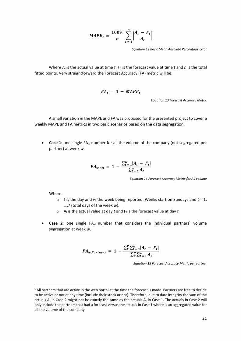
Forecast Accuracy Metrics

There are several metrics to measure the accuracy of the forecast. The choice of the

metric is problem specific. The most common metrics are presented in De Gooijer and Hyndman

(2006) paper, where the Mean Absolute Percentage Error (MAPE) is the preferred due to the

easy interpretability. Using the Actuals as the denominator, based on the rationality pointed by

Green and Tashman (2009), the basic MAPE form is the following:

21

𝑴𝑨𝑷𝑬𝒕 = 𝟏𝟎𝟎%

𝒏 ∑ |

𝑨𝒕 − 𝑭𝒕

𝑨𝒕|

𝒏

𝒕 = 𝟏

Equation 12 Basic Mean Absolute Percentage Error

Where At is the actual value at time t, Ft is the forecast value at time t and n is the total

fitted points. Very straightforward the Forecast Accuracy (FA) metric will be:

𝑭𝑨𝒕 = 𝟏 − 𝑴𝑨𝑷𝑬𝒕

Equation 13 Forecast Accuracy Metric

A small variation in the MAPE and FA was proposed for the presented project to cover a

weekly MAPE and FA metrics in two basic scenarios based on the data segregation:

• Case 1: one single FAw number for all the volume of the company (not segregated per

partner) at week w.

𝑭𝑨𝒘,𝑨𝒍𝒍 = 𝟏 − ∑ |𝑨𝒕 − 𝑭𝒕|𝒘

𝒕 = 𝟏

∑ 𝑨𝒕𝒘𝒕 = 𝟏

Equation 14 Forecast Accuracy Metric for All volume

Where:

o t is the day and w the week being reported. Weeks start on Sundays and t = 1,

…,7 (total days of the week w).

o At is the actual value at day t and Ft is the forecast value at day t

• Case 2: one single FAw number that considers the individual partners1 volume

segregation at week w.

𝑭𝑨𝒘,𝑷𝒂𝒓𝒕𝒏𝒆𝒓𝒔 = 𝟏 − ∑ ∑ |𝑨𝒕 − 𝑭𝒕|𝒘

𝒕 = 𝟏𝑷𝒌

∑ ∑ 𝑨𝒕𝒘𝒕 = 𝟏

𝑷𝒌

Equation 15 Forecast Accuracy Metric per partner

1 All partners that are active in the web portal at the time the forecast is made. Partners are free to decide to be active or not at any time (include their stock or not). Therefore, due to data integrity the sum of the actuals At in Case 2 might not be exactly the same as the actuals At in Case 1. The actuals in Case 2 will only include the partners that had a forecast versus the actuals in Case 1 where is an aggregated value for all the volume of the company.

22

Where:

o t is the day and w the week being reported. Weeks start on Sundays and t = 1,

…,7 (total days of the week w).

o At is the actual value at day t and Ft is the forecast value at day t

o P is the total partners included in the forecast released that meet the condition

that At > 0

o k is an individual partner that meets the condition that At > 0

V. Diagnosis of the Current Situation

24

General Concepts

In order to create and analyze an order forecast of the company, some basic concepts

are needed to be explained. These terminologies will keep showing up along the presented

report.

• As Is process: refers to the current forecast process or the processed followed by the

company after the proposed solution is fully implemented.

• Company: refers to the company in which the project is developed, that due to data

protection, won’t be called by the company official’s name.

• Web Portal: online retail web page created by the company, in which a potential

customer can explore the products and make a purchase.

• Products or items: refers to an individual product sold in the web portal. Each product

or item have their own attributes coming from a boutique or brand.

• Boutique: type of partner of the company, referring to designers or stablished stores all

around the world. These boutiques generally have their physical store (s) with their own

sales following independent marketing strategies. At the same time, as partners of the

company, they have sales done via the company’s web portal. These types of sales,

follow the company’s marketing strategies.

• Brand: type of partner of the company, referring to bigger fashion companies all around

the world. These brands generally do not have their own physical store (s) but they have

their own retail intermediate partners to sell their products. They have the particularity

that they have independence of their marketing strategies (they could follow or not the

company’s strategies).

• Portal Order: refers to the final purchase done by a customer in the web portal. These

portal orders can contain one or more items from a mix of different boutiques or

brands. The customer makes the payment based on the total amount of a portal order.

• Boutique/Brand Order: refers a purchase done by a customer organize by a specific

boutique or brand. As explained in the Scope and Limitations section, the presented

project will cover this type of order to make a forecast process.

• Marketing and Sale Calendar: refers to a day-by-day calendar with the specific sale

strategies that the company decide for each type of geo-group and customer tier. The

calendar contains sale promotions with the intention of accomplish the company’s

targets.

• x10/x20: type of sale referring the percentage of discount offered in the web portal for

all or specific items. For example, if the discount is 10%, the strategy is called “x10”.

• Black Friday (BF): type of sale referring to the typical extra discounts happening in the

weekend after the Thanksgiving celebration in United States (US). This sale type, is

applied in the entire world (not just US) and usually start on the Thanksgiving’s Thursday

and finishes in the Tuesday of the week after (includes the Cyber Monday).

• Singles Day (SD): type of sale referring to the extra discounts happening in Asia area

celebrating the pride of being single.

• Marketing Geo-groups: included in the Marketing and Sale Calendar, refers to clusters

of countries in which the customer is located. Therefore, each Marketing Geo-group

has their own marketing strategy.

25

• Shipping Location: country where the item (s) will be shipped, predefined by the

customer. Based on this information, the Marketing Geo-groups are created.

• Store Location: country where the boutique or brand is located at the time that ships

an item to the customer’s shipping location.

• Sale Season Forecast: type of forecast that include the months of official sales. This type

of forecast can be:

o Spring-Summer (SS) for the months of May, June and July.

o Autumn-Winter (AW) for the months of November, December and January.

• Full Price Forecast: type of forecast that include the months with no official sales,

therefore, the items usually are sold at full price with no discounts. However, this is not

a rule: if Sales and Marketing decide it, this time-period can include or not discounts for

specific days.

• Customer Tier: refers to cluster (tier) of type of customers. This type is defined at the

moment that a customer creates his or her account in the company’s web portal and

based on the characteristics of the customer. The Marketing and Sale Calendar have a

different strategy for each tier. For data protection purposes, the customer tiers will be

called Customer Tier 1, Customer Tier 2 and Customer Tier 3.

• Store Tier: depending on the level of importance (sales amount or marketing strategy),

the boutiques and brands are classified in store tiers. For boutiques, the classification

starts with a letter “T” plus a number (from 0 to 3). For brands, the letter is “B” plus a

number (from 0 to 3). The highest level of importance refers to the number 0 and the

less to 3.

• Data Warehouse (DW): main data source in which the forecast gathers the historical

boutique/brand Orders. The name of the DW used is BI_DW (Business Intelligence Data

Warehouse).

• Actuals: refers to the historical data available for a boutique or brand. For the project,

usually are actual boutique/brand order in a specific time granularity.

As Is Process

Marketing and Sale Calendar

As explained in the concepts section, the Marketing and Sale Calendar refers to a day-

by-day calendar with the specific sale strategies that the company decide for each type of geo-

group and customer tier. At this current state, this is manual file done in google sheets and is

owned by the Sales team. The following figure show a simulated example of a Marketing and

Sale calendar from November, 13th to December, 1st :

26

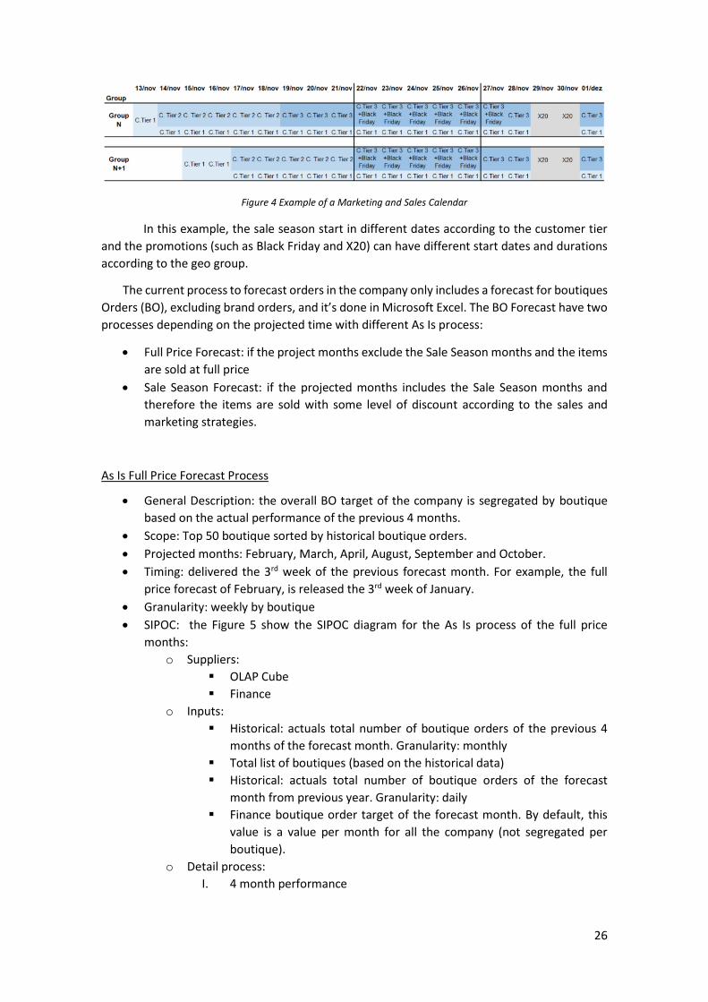
Figure 4 Example of a Marketing and Sales Calendar

In this example, the sale season start in different dates according to the customer tier

and the promotions (such as Black Friday and X20) can have different start dates and durations

according to the geo group.

The current process to forecast orders in the company only includes a forecast for boutiques

Orders (BO), excluding brand orders, and it’s done in Microsoft Excel. The BO Forecast have two

processes depending on the projected time with different As Is process:

• Full Price Forecast: if the project months exclude the Sale Season months and the items

are sold at full price

• Sale Season Forecast: if the projected months includes the Sale Season months and

therefore the items are sold with some level of discount according to the sales and

marketing strategies.

As Is Full Price Forecast Process

• General Description: the overall BO target of the company is segregated by boutique

based on the actual performance of the previous 4 months.

• Scope: Top 50 boutique sorted by historical boutique orders.

• Projected months: February, March, April, August, September and October.

• Timing: delivered the 3rd week of the previous forecast month. For example, the full

price forecast of February, is released the 3rd week of January.

• Granularity: weekly by boutique

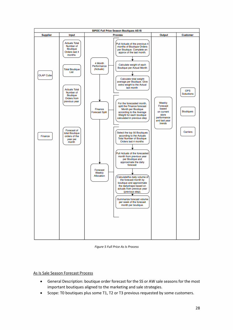
• SIPOC: the Figure 5 show the SIPOC diagram for the As Is process of the full price

months:

o Suppliers:

▪ OLAP Cube

▪ Finance

o Inputs:

▪ Historical: actuals total number of boutique orders of the previous 4

months of the forecast month. Granularity: monthly

▪ Total list of boutiques (based on the historical data)

▪ Historical: actuals total number of boutique orders of the forecast

month from previous year. Granularity: daily

▪ Finance boutique order target of the forecast month. By default, this

value is a value per month for all the company (not segregated per

boutique).

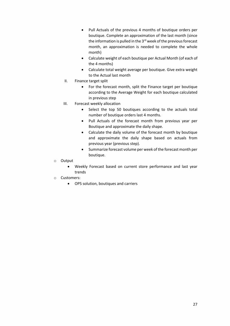
o Detail process:

I. 4 month performance

27

• Pull Actuals of the previous 4 months of boutique orders per

boutique. Complete an approximation of the last month (since

the information is pulled in the 3rd week of the previous forecast

month, an approximation is needed to complete the whole

month)

• Calculate weight of each boutique per Actual Month (of each of

the 4 months)

• Calculate total weight average per boutique. Give extra weight

to the Actual last month

II. Finance target split

• For the forecast month, split the Finance target per boutique

according to the Average Weight for each boutique calculated

in previous step

III. Forecast weekly allocation

• Select the top 50 boutiques according to the actuals total

number of boutique orders last 4 months.

• Pull Actuals of the forecast month from previous year per

Boutique and approximate the daily shape.

• Calculate the daily volume of the forecast month by boutique

and approximate the daily shape based on actuals from

previous year (previous step).

• Summarize forecast volume per week of the forecast month per

boutique.

o Output

• Weekly Forecast based on current store performance and last year

trends

o Customers:

• OPS solution, boutiques and carriers

28

Figure 5 Full Price As Is Process

As Is Sale Season Forecast Process

• General Description: boutique order forecast for the SS or AW sale seasons for the most

important boutiques aligned to the marketing and sale strategies.

• Scope: T0 boutiques plus some T1, T2 or T3 previous requested by some customers.

29

• Projected months: SS months (May, June and July) and AW months (November,

December and January)

• Timing: delivered the 2nd week of the previous month from the 1st month of the Sale

Season period. For example, the AW forecast, is released the 2nd week of October, as

the AW season start on November. This release day have several dependencies (release

of some required input data)

• Granularity: daily by boutique

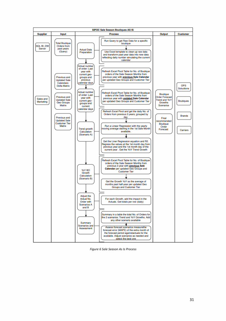
• SIPOC: the Figure 6 show the SIPOC diagram for the As Is process of the sale season

months:

o Suppliers:

▪ BI_DW data warehouse

▪ Sales and Marketing

o Inputs:

▪ Historical: Total boutique orders from past years (pulled in by a query

in Sever Management Studio). Is possible, 3 years of historical.

▪ Previous and current marketing and sale calendar. For example, for

AW18 forecast, is required the AW18 (current) and AW17 (previous)

sale calendars.

▪ Previous and current marketing geo-groups.

▪ Previous and current customer tier.

o Detail process:

I. Actual data preparation

• Run query to get raw historical data for a specific boutique.

• Use Excel template to clean up raw data: creates new columns

to transform past year data into new data reflecting daily

number simulating the current calendar. This is done

segregated by customer tiers and geo groups.

II. Actual number of order: Last year with current geo-groups and previous

calendar days.

• Refresh excel pivot table for number of boutique orders of the

sale season months plus one extra month 2 (called “forecast

period”) from previous year with previous sale calendar per

updated geo-groups and customer tier.

III. Actual number of order: Last year with current geo- groups and current

calendar days.

• Refresh excel pivot table for number of boutique orders of the

forecast period from previous year with current sale calendar

per updated geo-groups and customer tier.

IV. Trend growth Calculation (scenario A)

• Refresh excel pivot table and get the daily number of orders

from previous 3 years, grouped by day.

• Run a Linear Regression with the yearly moving average starting

in the 1st sale month available.

2 This extra month refers to the previous month to the sale season first’s month. For example, for AW this previous refers to the sale months (November, December and January) plus the previous one (October). Therefore, the total forecast period will be 4 months. This extra month will be used to assess accuracy of the forecast in following steps.

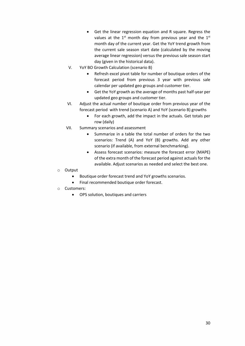
30

• Get the linear regression equation and R square. Regress the

values at the 1st month day from previous year and the 1st

month day of the current year. Get the YoY trend growth from

the current sale season start date (calculated by the moving

average linear regression) versus the previous sale season start

day (given in the historical data).

V. YoY BO Growth Calculation (scenario B)

• Refresh excel pivot table for number of boutique orders of the

forecast period from previous 3 year with previous sale

calendar per updated geo groups and customer tier.

• Get the YoY growth as the average of months past half-year per

updated geo groups and customer tier.

VI. Adjust the actual number of boutique order from previous year of the

forecast period with trend (scenario A) and YoY (scenario B) growths

• For each growth, add the impact in the actuals. Get totals per

row (daily)

VII. Summary scenarios and assessment

• Summarize in a table the total number of orders for the two

scenarios: Trend (A) and YoY (B) growths. Add any other

scenario (if available, from external benchmarking).

• Assess forecast scenarios: measure the forecast error (MAPE)

of the extra month of the forecast period against actuals for the

available. Adjust scenarios as needed and select the best one.

o Output

• Boutique order forecast trend and YoY growths scenarios.

• Final recommended boutique order forecast.

o Customers:

• OPS solution, boutiques and carriers

31

Figure 6 Sale Season As Is Process

32

As Is Performance

Part of this project is to propose a standard performance measurement process to

monitoring and leverage the continuous improvement cycle. Aligned to the literature review

chapter IV: Forecast Accuracy Metrics the 2 cases of Forecast Accuracy (FA) were proposed for

all volume and segregated by partner (refer to equations number 14 and 15). The data available

of the As Is processes include:

• Full price forecast: August, September and October 2018

• Sale season forecast: November and December 2018 (AW18 season)

In order to ensure significance in the conclusions, the way the results are presented and

summarized will be as the following:

• Forecast Accuracy (FA) for All Volume: refers to the performance of the forecast for all

volume of the company (without partner segregation) using Equation No. 14

• Forecast Accuracy (FA) Per Partner segregation: will be using the Top 3 partners based

on the actual boutique orders of the period (highest volume). Normally, these Top 3

boutiques remain the same during the year. Metric will be using the Equation No. 15.

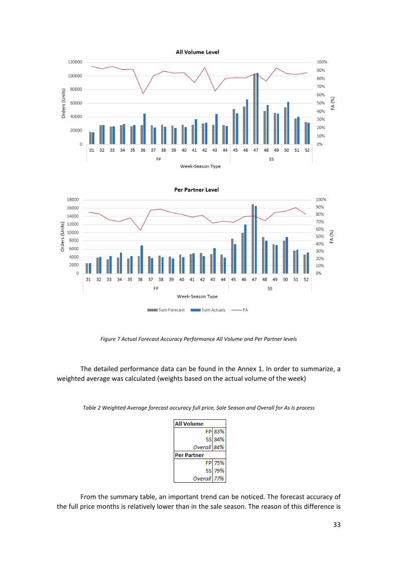
The following figures show the performance of the full price (FP) and sale season (SS)

forecast performance for All Volume followed by the Per Partner levels:

33

Figure 7 Actual Forecast Accuracy Performance All Volume and Per Partner levels

The detailed performance data can be found in the Annex 1. In order to summarize, a

weighted average was calculated (weights based on the actual volume of the week)

Table 2 Weighted Average forecast accuracy full price, Sale Season and Overall for As Is process

From the summary table, an important trend can be noticed. The forecast accuracy of

the full price months is relatively lower than in the sale season. The reason of this difference is

34

due to the limitations of the current process: as explained in the previous section, the full price

process is not a real forecast, but a segregation of the finance target orders per boutique based

on actuals. For the All volume scenario, in the Figure 7 it can be easily seen 3 main drops in the

Forecast Accuracy metrics in the weeks 36, 41 y 43. Similar case happens in the Partner in week

36. The main explanations on the FA for the full price days, is that Sales and Marketing released

last minute X20 sale promotions, creating peaks of sales not included in the forecast when it was

released. These last-minute promotions are seen very often in the company.

In the case of sale season forecast accuracy, usually the FA is better than the FA in full

price. The improvement of the performance is driven by a more statistical process and the

capability of re -adjust if needed. During the AW18 sale season, 7 forecasts were released driving

by last minute promotion campaign changes or management decisions. The following tables

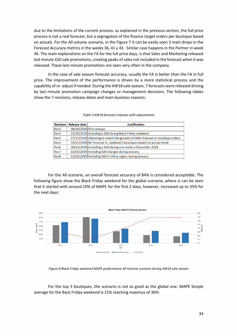
show the 7 revisions, release dates and main business reasons:

Table 3 AW18 forecast releases with adjustments

For the All scenario, an overall forecast accuracy of 84% is considered acceptable. The

following figure show the Black Friday weekend for the global scenario, where is can be seen

that it started with around 10% of MAPE for the first 2 days, however, increased up to 35% for

the next days:

Figure 8 Black Friday weekend MAPE performance All Volume scenario during AW18 sale season

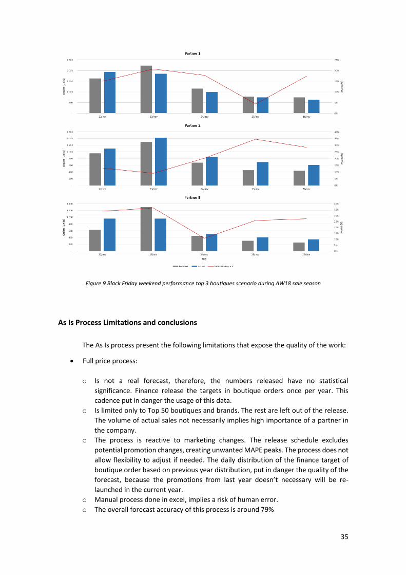
For the top 3 boutiques, the scenario is not as good as the global one. MAPE Simple

average for the Back Friday weekend is 21% reaching maximus of 36%:

35

Figure 9 Black Friday weekend performance top 3 boutiques scenario during AW18 sale season

As Is Process Limitations and conclusions

The As Is process present the following limitations that expose the quality of the work:

• Full price process:

o Is not a real forecast, therefore, the numbers released have no statistical

significance. Finance release the targets in boutique orders once per year. This

cadence put in danger the usage of this data.

o Is limited only to Top 50 boutiques and brands. The rest are left out of the release.

The volume of actual sales not necessarily implies high importance of a partner in

the company.

o The process is reactive to marketing changes. The release schedule excludes

potential promotion changes, creating unwanted MAPE peaks. The process does not

allow flexibility to adjust if needed. The daily distribution of the finance target of

boutique order based on previous year distribution, put in danger the quality of the

forecast, because the promotions from last year doesn’t necessary will be re-

launched in the current year.

o Manual process done in excel, implies a risk of human error.

o The overall forecast accuracy of this process is around 79%

36

• Sale season process:

o Is limited only to T0 boutiques that represent around 2% of all the partners. Also,

does not include brands. This has caused complains from the excluded partners

putting in danger the image of the company.

o The simple but large manual work done in excel, limits the inclusion more partners

and the capacity to perform quick adjustments. Also, increase the risk of human

error. Even though, 7 forecasts were released, representing large human working

hours to make these adjustments. The amount of time consumed in recreating the

excel sheets, limits the time available to high value-added activities, such as the

analytic part for better decision making.

o Poor adjustment to real time marketing campaign changes or to create what if

analysis for better decision making.

o Basic statistical analysis is performed in the process, limited to year over year (YoY)

growths and linear regression. The process fails if not enough historical data is

available.

o The process does not include any monitoring sub process nor have any scorecard

with standard KPIs and data visualization for the analyst and internal customers of

the forecast.

o The process is considered not robust and reactive to marketing changes.

o The overall forecast accuracy of this process is around 81%.

Root Cause Analysis

Using a lean manufacturing tool, the root cause analysis will use a Cause and Effect

diagram 3 in order to show the complete picture of the possible causes that creates the problem

statement. This analysis will help prioritizing the causes and make sure the real cause (called

root cause) is being solved in the solutions.

The diagram uses 6 categories to analyze the possible causes. Next, the categories

explain followed by the diagram:

• Method: refers to the processes and methodologies used

• Materials: in this case, refers to the input data used in the processes

• Measurement: refers on KPIs used to check the performance of the processes.

• Environment: refers to the work space and cultural organization of the company.

• Manpower: refers to the human resources performing the tasks.

• Tools: in this case, refers to the software and other tools used to perform the processes.

3 Also called Ishikawa diagram or fishbone diagram, created by Kaoru Ishikawa that show the causes of a specific event.

37

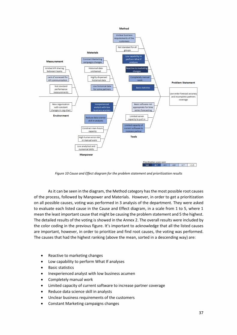
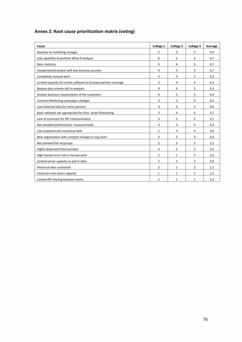
Figure 10 Cause and Effect diagram for the problem statement and prioritization results

As it can be seen in the diagram, the Method category has the most possible root causes

of the process, followed by Manpower and Materials. However, in order to get a prioritization

on all possible causes, voting was performed in 3 analysis of the department. They were asked

to evaluate each listed cause in the Cause and Effect diagram, in a scale from 1 to 5, where 1

mean the least important cause that might be causing the problem statement and 5 the highest.

The detailed results of the voting is showed in the Annex 2. The overall results were included by

the color coding in the previous figure. It’s important to acknowledge that all the listed causes

are important, however, in order to prioritize and find root causes, the voting was performed.

The causes that had the highest ranking (above the mean, sorted in a descending way) are:

• Reactive to marketing changes

• Low capability to perform What If analyses

• Basic statistics

• Inexperienced analyst with low business acumen

• Completely manual work

• Limited capacity of current software to increase partner coverage

• Reduce data science skill in analysts

• Unclear business requirements of the customers

• Constant Marketing campaigns changes

38

• Low historical data for some partners

• Basic software not appropriate for time series forecasting

• Lack of scorecard for KPI communication

As a matter of conclusion, the solutions of the problem statement, must ensure that this

list is covered in the design of the new process in order to ensure the success of the project.

VI. Problem Solution

40

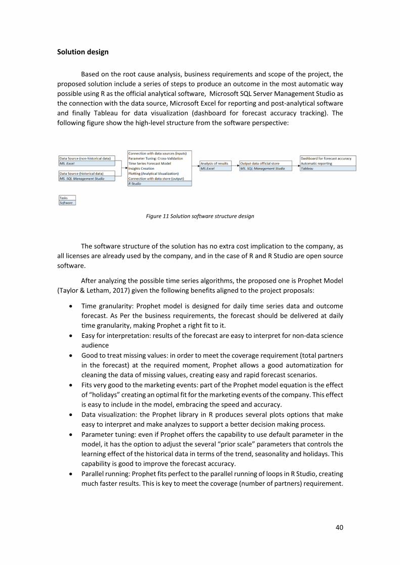
Solution design

Based on the root cause analysis, business requirements and scope of the project, the

proposed solution include a series of steps to produce an outcome in the most automatic way

possible using R as the official analytical software, Microsoft SQL Server Management Studio as

the connection with the data source, Microsoft Excel for reporting and post-analytical software

and finally Tableau for data visualization (dashboard for forecast accuracy tracking). The

following figure show the high-level structure from the software perspective:

Figure 11 Solution software structure design

The software structure of the solution has no extra cost implication to the company, as

all licenses are already used by the company, and in the case of R and R Studio are open source

software.

After analyzing the possible time series algorithms, the proposed one is Prophet Model

(Taylor & Letham, 2017) given the following benefits aligned to the project proposals:

• Time granularity: Prophet model is designed for daily time series data and outcome

forecast. As Per the business requirements, the forecast should be delivered at daily

time granularity, making Prophet a right fit to it.

• Easy for interpretation: results of the forecast are easy to interpret for non-data science

audience

• Good to treat missing values: in order to meet the coverage requirement (total partners

in the forecast) at the required moment, Prophet allows a good automatization for

cleaning the data of missing values, creating easy and rapid forecast scenarios.

• Fits very good to the marketing events: part of the Prophet model equation is the effect

of “holidays” creating an optimal fit for the marketing events of the company. This effect

is easy to include in the model, embracing the speed and accuracy.

• Data visualization: the Prophet library in R produces several plots options that make

easy to interpret and make analyzes to support a better decision making process.

• Parameter tuning: even if Prophet offers the capability to use default parameter in the

model, it has the option to adjust the several “prior scale” parameters that controls the

learning effect of the historical data in terms of the trend, seasonality and holidays. This

capability is good to improve the forecast accuracy.

• Parallel running: Prophet fits perfect to the parallel running of loops in R Studio, creating

much faster results. This is key to meet the coverage (number of partners) requirement.

41

The design of the solution has an administrative overall process (called Step 0) and 6

technical steps process (some optional and other required) to ensure the business requirement

are met and the root cause of the problem statement covered. The high-level steps are shown

in the next figure, followed by sections explaining with detail each step:

Figure 12 Overview of the Solution steps

Step 0: Overall Administrative Process

The overall administrative procedure is designed to attack the problem statement with

a robust and trustful process as the following:

• Owner: Supply Chain Analytics.

• Forecast release cadence: weekly releases every Thursday end of day.

• Forecast timeframe: 7 weeks ahead starting the week after the release. Every new

release will include one extra week at the end of the horizon and will refresh the forecast

of the weeks that are shared in the previous release. The following figure show the logic

graphically:

Figure 13 Solution forecast release schema

• Forecast graduality:

o Time unit: day

42

o Locations: partners and all company volume

• Forecast coverage: all partners (boutiques and brands, approximate this represent 1200

partners) that has at least 7 weeks of historical data plus the overall “all” company

volume.

• Forecast release formats: excel sheet and loaded in BI_DW.

• Communication method: e-mail with a pre-defined distribution list.

• Forecast accuracy and monitoring results dashboard 4 : the forecast accuracy will include

two measures depending of the locations: all volume forecast accuracy and overall

partners forecast accuracy.

The proposed overall administrative process is intended to be able to capture all

marketing events in a proactive way, increasing the accuracy and creating trust of the partners

and internal customers of the forecast by having the proposed cadence release and partner

coverage. Also, will create one single source of truth of the order forecast data by centralizing

the ownership, data release channel and standard formatting.

The following sections of this chapter will explain more the “how” of the solution from

a more technical point of view and show the preliminary results of the solution, making a

benchmarking against other methodologies (using the current As Is method and ARIMA) with

the intention of showing the suitability and trust in the proposed solution. Finally, a proposed

dashboard for monitoring the results will be explained in the last section, in order to track and

share the results.

Step 1: Data Preparation

The data preparation phase is intended to ensure all necessary information and data is

ready and clean to continue to the following phases. As usual, the data needs to be cleaned and

structured for data quality purposes. In this phase, the raw data is transformed and merged with

other data sources. The step by step diagram is shown in the next figure followed by the detail

description of the steps:

4 Details of the data included the outcome of the forecast are explained in the following section of the present chapter: Forecast Release Table.

43

Figure 14 Step 1: Data Preparation flow

Sub Step 1.1: Load data sources

• Objective: load R libraries and raw data from data sources: R packages and BI_DW and

excel documents.

• Tasks:

1. Install and load all necessary packages and libraries in R Studio. The required

packages and libraries are listed in the Annex 3. This loading is required to

ensure no failure will happen during the rest of the model.

2. Load Geo-groups vs Countries matrix file from local disk (excel document):

previously prepared, this excel document is loaded as a CSV into the R Studio

code and contains all the countries of the customers that the company has. Each

country has a geo-group classification. This classification is defined by Sales and

Marketing team. The rationality is that each geo-group will have a different

marketing strategies (events). Therefore, the forecast needs to be personalized

by geo-group. The following is a high-level description of the geo-groups:

▪ Group 1a: LATAM area.

▪ Group 1b: North America area except Mexico.

▪ Group 2a: Asia area except Japan and Singapore.

▪ Group 2b: Japan and Singapore.

▪ Group 3: ROW (rest of the word)

▪ Group 4a: United Kingdom

▪ Group 4: Spain

44

▪ Group 5: Italy and Belgium.

▪ Group 6: France

▪ Group 7: Russia

3. Load 4 years of historical daily orders data per shipping country per partner and

partner type from BI_DW. Historical data will include the day, order, partner

name and partner type (boutique or brand). General rule is 4 years of historical

data; however, this will depend on the time that the partner has been with the

company (could be less for more recently joined partners).

4. Load GMV Forecast from local disk (optional) as an excel CSV document. This

information is released by Finance once per month and contains the forecast of

the GMV for all the company (not per partner) per day. Usually only include 1

month ahead from the release date. This information is optional, as is not an

input to make the order forecast but is used as an insight information for

benchmarking purposes (explained with more details in the Step 4: Insights)

5. Load Holidays for each geo-group from local disk as an excel CSV document. This

information are all the marketing events in the past and future (if known) for

each individual geo-group according to the Sales and Marketing campaign

calendar. Holidays is the terminology used following the Prophet library

however, in this case, more than a holiday, it is a marketing promotion, such as

X20, Black Friday weekend or a VIP customer tier sale season. The document

includes the name of the Holiday, date and geo-group.

6. Load best parameters for the forecast model from local disk (optional) as an

excel CSV document. This information refers to the parameters (called “best

parameters”) that Prophet model will use to make the forecast. This is optional,

as the user can run Prophet model with the default parameters. To obtain these

best parameters, the Step 2 (Cross Validation) need to be performed first

(explained with more detail in the Step 2)

7. Load 2 years historical Stock Level end of day per season per partner per day

from BI_DW (optional). This information comes from a query and is not a

required information to run the Prophet model (same case as the GMV

Forecast). This information is only used as extra insight data used in the Step 4

(Insights).

Sub Step 1.2: Prepare and clean data sources

• Objective: Do a general cleanup of the data, remove unnecessary information and

generate structure in the data.

• Tasks:

1. Assign Geo-Group to historical order data: this is done through a join function,

where the order historical data is merged with the geo-groups CSV file loaded

in the previous steps. The join is done by the shipping country. The outcome will

be the historical data including the geo-group depending on the shipping

country (that refers where the customer is)

2. Clean up data formats for standard data types (for example, Date type as

DD/MM/YYYY)

45

3. Remove unnecessary columns from data frames

Sub Step 1.3: Global model parameter selection and definition

• Objective: user needs to select some options to run the model based on the objectives

of the outcome.

• Tasks:

1. Define global parameters and select model options. This section is user-based,

meaning that the user needs to input in the model some information required

to run it. The options selected will answer the following questions:

▪ Forecast horizon (integer): how many days does the user want to

forecast? Always the time unit is days.

▪ Insights (Binary: True-False): does the user want to include insights

(Step 4) in the forecast or not? This decision implies around of 30% more

of computer performance and time to run the model, but the benefit is

to have more information to support a better decision making process.

▪ All Company (Binary: True-False): does the user want to run the model

for all the company volume (one single forecast for all the partners as a

whole) or does the user want to run the model for each individual

partner?

▪ Export (Binary: True-False): does the use want to export a CSV

document with the output forecast into the local device?

▪ Text options to be printed in the outcome file:

• Scenario Name

• Scenario Revision

• Release Week

Sub Step 1.4: Failure mode adjustment and validation

• Objective: provide a general check that no information is missing to run the model

without errors.

• Tasks:

1. Validate all countries in the historical data have a geo-group assigned. In case a

new country is included in the historical data, this validation will make a check

that all countries have a geo-group defined. If a country is found without a geo-

group, will print a message of warning.

2. Create empty data frame for forecast horizon. This is a data frame with zero

values in all the forecast horizon. This will ensure that the model won’t crush in

case no historical data is available for a specific partner and geo-group.

46

Step 2: Cross Validation

The Cross-Validation phase is intended to maximize the forecast accuracy by splitting

the historical data in training (70%) and test (30%) data set, then train different models (each

model with a possible combination of Prophet parameters). Finally measure the performance of

each model with the test data set, in order to select the model with the lowest error. The step

is optional as the user can decide to use the default Prophet parameters. The benefit is implying

a better model and better accuracy; however, this Step takes a long period of time to run due

to the heavy performance driven by the amount of training models and validation. The user can

perform this Cross-Validation in two ways:

• Cross-Validation for each partner type: boutique, brand and all company volume. This

option takes approximate 18 hours to finish. This partner type generalization is the most

used option as it provides reasonable results and the required time to run it is

manageable.

• Cross-Validation for each individual partner: This option takes approximate 6 hours to

finish on single partner. This option might be useful for the highest volume partners that

highly impact the overall company forecast accuracy levels.

Even with the long performance time this step takes, the benefit is worth it. Also, the

results aren’t highly sensitive to short amount of times. This mean, that the user can run this

step once per month and reuse the best parameters for all the weekly forecast releases. The

final outcome will be a data frame exported as a CSV document with the best parameters of the

Prophet model per partner type (or individual partner) per geo-group. The parameters and

values to be tested are the following:

• n.changepoints: 20, 25 (default), 30

• holidays.prior.scale: 5, 10 (default), 15

• seasonality.prior.scale: 5, 10 (default), 15

• Seasonality mode: “additive” (default), “multiplicative”

The step by step diagram is shown in the next figure followed by the detail description

of the steps:

47

Figure 15 Step 2: Cross Validation

Sub Step 2.1 Data split in partner type

• Objective: prepare the data by splitting and aggregating it according to the desired

output

• Tasks:

1. Split historical order data per partner type and geo-group

2. Aggregate total orders per day

Sub Step 2.2 Prepare parameters combination matrix

• Objective: create all the possible combinations of Prophet parameters. Each of these

combinations will be a model to be trained and validated.

• Tasks:

1. Create a matrix grid of several possible combinations of different parameters of

Prophet model

Sub Step 2.3 Perform a cross validation and measure error

• Objective: perform the cross validation to measure the error in all possible

combinations.

48

• Tasks (for each partner type and geo-group):

1. Split data in training (70%) and Test (30%)

2. Perform cross validation models for each combination of parameters of the

matrix grid

3. Measure the MAPE and other metrics in the Test data set.

4. Calculate MAPE average of the test data set and store results

Sub Step 2.4 Selection of best parameters per partner type

• Objective: select the best parameters based on the minimum MAPE model.

• Tasks:

1. Select the minimum MAPE for each combination of a geo-group and partner

type

2. Store results as Best Parameters and export it in a CVS file in the local disk

Step 3: Forecast

This is the core step of the process where the forecast is generated for the horizon pre-

defined by the user. The forecast can include or not insights and can use the best parameters to

maximize the accuracy. As explained before, each partner’s historical data will be segregated by

geo-group and a forecast will be create for each group. Then, merging them into one single

partner forecast. The rationality is that the forecast is highly sensitive to the marketing campaign

events (called “Holidays” in the Prophet model). The marketing events are different per region

(Singles Day promotion, for example, only happen in China Region), therefore, in order to

increase the accuracy, each partner will have 10 different forecasts (one per for each geo-group).

This will make the performance running time 10 times longer than if one single forecast is

created per partner, however, the accuracy will be degraded. The step by step diagram is shown

in the next figure followed by the detail description of the steps:

49

Figure 16 Step 3: Forecast

Sub Step 3.1 Data split per partner and geo-group

• Objective: prepare the data by splitting it by partner (if this option was selected. If all

company volume is selected, then the data won’t be segregated per partner) and then

by geo-group.

• Tasks:

1. Through 2 nested loops, the historical data will be segregated first by partner

and then by geo-group

Sub Step 3.2 Forecast creation for each case

• Objective: create the forecast for the pre-defined horizon.

• Tasks:

1. Assign Prophet model parameters from Best Parameters file (depending on

Partner Type and geo-group) from Cross Validation or use default ones.

2. Perform some failure model validations, such in case there is no historical data,

then the empty data frame will be assigned to that specific geo-group and

partner.

3. Perform Prophet model and forecast for the horizon.

50

4. Store results in a data frame for the geo-group

5. Merge all geo-group forecast into one summary forecast file for a partner

Sub Step 3.3 Create summary files

• Objective: merge all forecast of each individual partner into one single data frame.

• Tasks:

1. Append each Partner forecast into the CSV summary file. Export it into the local

device if user selected in the global model parameters.

Step 4: Insights

The insights phase is an optional process that produce extra information in the forecast

output, in order to support the analytical process (following step) for a better decision-making

process. As mentioned before in the sub step 1.3, the user can enable or disable this feature as

a global parameter in the model. Including the insight will produce a slower performance time

but will create more information. Depending on the user objective, this feature will be used or

not. The step by step diagram is shown in the next figure followed by the detail description of

the steps and insights:

Figure 17 Step 4: Insights

51

Sub Step 4.1 Create forecast insights

• Objective: produce 2 insights (YoY change and GMV to order forecast) to the normal

forecast to support the analytics phase.

• Tasks:

1. Produce the Year over Year (YoY) change: produce the relative percentage of

change from a forecasted day versus the previous year same day actual value.

For example, an insight YoY value of 30% in November, 3rd of 2019 means that

there is a growth of 30% from the historical value in November, 3rd of 2018 and

the forecasted value calculated by the model. This information, help understand

the general change of a forecast.

2. Produce the GMV to order forecast transformation (value, lower value and

upper value): the basic idea is to convert the GMV finance daily forecast (GMV

is measure in currency USD units) into an order forecast based on a forecasted

ratio GMV-order. This insight is where the majority of the performance

requirement of the insight option take place. As mentioned before, the GMV

forecast is provided by finance once per month in a daily granularity but is not

segregated by partner, only a whole GMV number for all the company value.

The rationality of this insight is to produce an alternative order forecast from

the main one produced in Step 3 and be able to compare it if needed. The

general logic to create this insight is the following:

▪ Calculate the GMV portion per partner based on the YTD (Year to Date)

historical GMV value.

▪ Estimate the GMV forecast per partner based on the portion calculated

in the previous step.

▪ Calculate the historical GMV-order ratio per day and per partner in the

previous 4 years. This will be the historical data of the forecast model.

▪ Estimate the GMV-order forecasted ratio value using the same Prophet

model algorithm explained in the Step 3.

▪ Covert the finance GMV forecast into order per day using the forecasted

ratio.

Sub Step 4.2 Merge insights with summary files

• Objective: merge insights created into the summary forecast data frame.

• Tasks:

1. Include YoY and GMV to order forecast to the summary order forecast file for

each partner

52

Step 5: Analysis and plots

The intention of this solution design is to provide a forecast in the most automatic and

accurate way to meet the company needs. However, as in any forecast process, the judgmental

phase of the analysist is highly important. This is based on the expertise of the analysist in the

industry. To help on this process, the insight option is available in the previous Step, but also,

some visuals can be printed to help on this phase. This step is also optional, as it not a

requirement to run the Prophet model. The step by step diagram is shown in the next figure

followed by the detail description of the type of plots:

Figure 18 Step 5: Analysis and plots

Sub Step 5.1 Visualize forecast and model assumptions

• Objective: merge insights created into the summary forecast data frame.

• Tasks:

1. Print plots included in prophet library for a forecast of a specific partner. The

most used plots are:

▪ Historical and forecast scatter-line plot: show the historical data by

black points and the model forecast by a blue line. The following figure

show an example:

53

Figure 19 Example Prophet historical and forecast scatter-line plot

▪ Forecast components: show the impact of the different components of

the forecast (trend, seasonality, holidays). The following figure show an

example:

Figure 20 Example Prophet forecast components plot

Sub Step 5.2 Plot forecast with insights

• Objective: produce personalized plots with extra insights for better forecast analysis.

• Tasks:

1. Include historical stock level (stock end of day) plot per season per partner (area

plot): this plot shows the stock level (in units) per seasons, with the intention to

understand the possible impact of the stock levels in the forecast.

54

2. Include the historical percentage of discounted stock plot per day (line plot):

this plot shows the portion (%) of the stock that was had any type of discount in

the historical data. For example, a value of 20% in this plot, means that for the

selected partner in that specific day, 20% of all their stock had any type of

discount.

3. Include the average discount rate plot (line plot) per day: this plot provides a

weighted average of the discount percentage that certain partner that in all of

the items per day. For example, a value of 20% in this plot, means that for the

selected partner in that specific day, from the stock of items that had any type

of discount, in average, the discount was 20% of the normal selling price.

4. Include the overall discount metric per day: this plot shows is the multiplication

of the previous 2 metrics (historical percentage of discounted stock times the

average discount rate). This metric will provide a combination of the previous 2

metrics to get an overall impact of the discounts: in stock levels and discount

value. The following figure show an example:

Figure 21 Example personalized plots with extra insights

55

Sub Step 5.2 Judgmental adjustments

• Objective: use analyst experience and knowledge (supported by the insights) for a

revision of the forecast and adjust it if needed.

• Tasks:

1. Analyze forecast, insights and plots to adjust forecast based on judgmental

decisions.

Step 6: Export and dashboard

Once the final forecast was been selected by the analyst, the next and final step will be

to upload it in the official data base to support the right storage and communication of this

information. This will ensure that the forecast will have one and only one single source of truth

in the organization, in a standard and structured format (detail on this data structure are

explained in the next section: Forecast Release Table). Then, a data visualization is required to

track the day to day forecast behavior against the actual performance by tracking the forecast

accuracy metric. This will be done through a simple yet complete dashboard, where the

information flow automatically from the data base to the dashboard using Tableau software.

The step by step diagram is shown in the next figure followed by the detail description of the

type of plots:

Figure 22 Step 6: Export and dashboard

Sub Step 6.1 Export results and load data base

• Objective: export official forecast result in the required formats for the proper

communication.

• Tasks:

56

1. Export forecast results into local disk as CSV forecast. This format is required as

some customers of the information does not use SQL Server to query

information.

2. Automatic load of forecast into BI_DW data base table. This is key for data

standardization and support the dashboard.

Sub Step 6.2 Refresh forecast monitoring dashboard

• Objective: provide a dashboard with forecast accuracy with automatic refresh cadence.

The details of the dashboard are explained in a following section of this chapter:

Forecast Accuracy and dashboard reporting.

• Tasks:

1. Refresh Tableau dashboard with new forecast release through automatic

linkage between Tableau and BI_DW. Updates must be done in a daily basis.

Sub Step 6.3 Communicate forecast release

• Objective: proper communicate the release of a new forecast to a pre-selected

distribution list (internal customers).

• Tasks:

1. Send communication of forecast release to the official distribution list using

electronic mail as the channel. The communication includes the following

sections:

▪ Forecast release week (called as Scenario Name)

▪ Highlights of the forecast: This section is optional, depending on the

analyst judgment to make a remark of any special situation, for

example, the inclusion of a new marketing event.

▪ Forecast terms and assumption

The following figure show an example of a normal forecast release communication e-

mail:

57

Figure 23 Example of a standard forecast release commutation e-mail

Forecast Release Table

To ensure the structure of the data, a standard table and data type is part of the solution.

This is key for the data integrity specially with the linkage with the forecast dashboard. The table

include 9 different fields and are explained in the following table:

Table 4 Forecast Release Table fields

58

Forecast Accuracy and dashboard reporting

The success of the forecast dashboard is to ensure the quality and integrity of the data.

The company uses Tableau as the official data visualization software for dashboard creation. Is

important to mention that the dashboard is designed for the internal customers. Is not intended

for the forecast analyst. Therefore, the dashboard is simple and easy to understand for any

audience. The following figures show the Tableau data source join table design:

Figure 24 Tableau join tables design for forecast dashboard

Basically, Tableau will connect to only two tables in BI_DW merged by “Date” and

“StoreKey” fields as the unique identifiers.

Figure 25 Example final forecast dashboard

The data sources are Fact Order Lines (FOL: for actuals) and Order Forecast (for the

forecast values). The first one (FOL), have two types sections based on the granularity (different

queries to pull in the information): one for each individual partner and another for All volume

of the company. This structure will pull and merge the information to create the proposed

dashboard. The following figure show an example of it:

59

Figure 26 Example final forecast dashboard (data protected)

The sections shown in the dashboard are:

1. Date slider: user can select the time frame required. Date units are the same as the

forecast: days.

60

2. View Actual Data: user can select weather or not to see the actual data and forecast

accuracy metric.

3. Scenario Name: user can select the scenario name, which refers to the forecast release

week.

4. Partner Location: user can select the All volume or by partner location.

5. Basic Statistics: show a basic descriptive (simple average, maximum and minimum

values, standard deviation) and the forecast accuracy and MAPE simple averages of the

time frame selected in the date slider.

6. Daily Forecast, Actual and Forecast Accuracy percentage: bar and line plot showing the

forecast and actual values (bars) and forecast accuracy (line).

7. Last Year Actual versus Forecast: provide Year over Year change percentage of the

forecast to the actual value from that exact day the previous year.

8. Weekly aggregated Forecast & Actual values and the simple daily average of the: bar

and line plot showing the sum of the forecast and actual values (bars) and forecast

accuracy (line) as the simple average of the daily forecast accuracy values within the

time frame selected in the date slider.

9. Time Series with the actual data (scatter point plot) from one year of historical plus the

forecast selected (line plot)

10. Forecast assumptions and terms: general explanation of the model and the most

important assumptions.

The dashboard’s administrator is the forecast data analyst in charge of creating the

forecast. The dashboard is updated every day at 00:00 hours and is shared as a link for public

access within the company. The link is included in the forecast communication e-mail. Also, the

dashboard has the capability to send automatic screenshots to a pre-defined distribution list.

This can be easily done by the administration under previous request.

VII. Results and Discussion

62

The new process was implemented since January 4th with the Top 50 partners. Then, the

number of boutiques keep increasing until reach a 100% of coverage by end of March 2019. The

data available for the 2 processes (As Is and new) are well represented and include the 2 types

of periods (Full Price and Sale Season). The As Is process include data from week 31 until week

52 of 2018. The new process was implemented from week 6 to week 26 of 2019 (by the time

this documented was written):

Table 5 Weeks available for Forecast Accuracy Comparisons

The forecast accuracy numbers where calculated using the Equations No. 14 and No. 15

for the All Volume and Per Partner, as explained in the Chapter IV (Literature Review). The

regular proposed process includes 100% of the partners for the Per Partner Forecast Accuracy

metric. For this case, the Per Partner metric includes only the Top 3 partners for data consistency

between the As Is and new processes. The detailed calculations can be found in Annex 1

Figure 27 Forecast Accuracy Comparisons As Is process with new (Prophet)

The figure show that Prophet model is has the best performance in all the cases except

the Top 3 Partners, however, this in reasonable as the AW18 Sale Season (using the As Is process)

was less complicated than SS19 (using Prophet). The amount and types of holidays used in SS19

has being new types, creating difficulties in the regression. Some remarks about this preliminary

results and comparisons are:

63

• In general, Prophet is performing in average 3% better than the As Is

process, especially against the Full Price months, where is performing up to

8% better.

• Considering the amount of manual work of the current process, Prophet can

perform higher number of partners in less amount of time with better

accuracy. The proposed solution estimates an order forecast automatically

in 1.83 minutes per partner versus approximate 15 minutes in previous

model (88% of time reduction).

• This time reduction allows to have more flexibility (quick What If analysis

and adjustments), quality (assign more time to high value-added analytical

activities) and coverage (our target to cover 100% of the partners).

• The geo-group forecast approach of the solution, allows fitting the

marketing events in a personalized way. The Holidays effect in the forecast,

solves the problem that Auto Arima has, which is, create smart peaks in the

future based on trained events from the past (like an X20 or Private Sale).

The following figure, show how the proposed solution adjust better to the

actual volume in the peak days when a marking event was modeled as a

Holiday input:

Figure 28 Daily Forecast Accuracy Prophet and Auto Arima

The proposed solution clearly states that the role of the analyst is key for the success of

the process. The preliminary results, for sure, can be improved as the analysist growth the

business knowledge in the industry. The Step 5 (Analysis and plots) has the intention to review

the outcome of the model and adjust if needed with extra insights (such stock and discount

levels). As the coverage will be 100% of the partners (as per the business requirements), is

obviously that making a revision for all the partners won’t be possible for one single analyst,

therefore, is suggested to implement a strategy of prioritization.

For the recommended target, is necessary more level of detail on the actual

performance. As explained in this chapter, the forecast process includes a forecast release each

64

week for 7 weeks ahead. Each forecast released in called “scenario”. The following figures show

the forecast accuracy for All Volume and Per Partner (Top 3) using the Equations No. 14 and 15

for each scenario in each forecasted week. The light blue frame refers to Full Price weeks and

the dark black Sale Season weeks (in this case: Spring Summer 2019):

Figure 29 Weekly performance of the proposed process (Prophet) for All volume (Global)

Figure 30 Weekly performance of the proposed process (Prophet) for Per Partner (Top 3)

65

As expected, the Forecast Accuracy is higher in the first weeks and decreases across the

horizon. Also, in both cases the majority of the forecasted weeks, the Full Price weeks perform

better than the Sale Season. As expected, the Sale Season weeks will always be harder to

forecast, due to the higher complexity in the holidays (marketing events) as the market keep

being more a more competitive. A small poll was done to understand from the point of view of

the partners and other customers, how many weeks in advance do they need to know the order

forecast in order to be prepared on time to fulfill the expected demand? The answer was around

2 to 3 weeks. Based on this feedback, the preliminary performance results and the continuous

improvement efforts of this model, a suggested bold but realistic target of forecast accuracy

would be around 90% for All company volume and 70% for individual partners, using the 4th

week of each forecast release.

VIII. Conclusions

67

• Time series decomposition approach of the solution allows an easy way of

interpretation of the forecast recommendation. Using Prophet methodology adjusted

with the geo-group forecast approach of the solution, allows fitting the marketing

events in a personalized way, increasing the probability of have a better forecast

accuracy.

• The End to End design of the solution deals with the data extraction, transformation,

analysis, forecasting, loading, distribution and visualization in an automatic way,

creating a robust and reliable process.

• The solution is a complete Business Intelligence platform: is connected with the official

data warehouse, ensuring the data integrity and security. Also, creates an automatic

Tableau dashboard with the visualization of the forecast and the actuals (including the

forecast accuracy metric).

• The performance of the proposed solution shows an average of 3% better accuracy than

the As Is process, especially against the Full Price months, where is performing up to 8%

better. As the model and knowledge from the analysis keeps evolving towards the luxury

fashion industry, the accuracy will keep increasing.

• The new process increases the partner coverage up to 100% having the capability to

create a forecast recommendation for all the partners (more than 1000) in short amount

of time. The proposed solution estimates an order forecast automatically in 1.83

minutes per partner versus approximate 15 minutes in previous model (88% of time

reduction).

• Obviously, this automatic End to End solution does not eliminate the analytical part of

the data scientist, but in fact, reinforces it. Allows to release time from the non-value

activities to focus in the high value-added ones (for example: tuning parameters,

deciding to use the lower or upper case based on stock levels, etc).

• Finally, using open source libraries and free high analytical software (R Studio) the

proposed solution doesn’t add any financial implication to the business.

IX. Limitations and Recommendations for Future

Works

69

• The business needs to reinforce the communication of the forecast, in order to create

trust. This process is considered as “new” for the majority of the partners, is

recommended to work in the distribution and usage of the forecast. In order to

maximize the benefits, the business need to ensure that the partners are using this

information for their capacity planning.

• The officialization and communication of marketing events from the Sales and

Marketing department is still consider slow. Even though the solution fits to the

marketing events per geo-groups, is still a customer of this information. Is

recommended to create awareness of the importance to release as fast as possible any

new or change marketing event.

• In order to improve the accuracy, some modifications in the proposed model can be

performed and tested. Is important to acknowledge that the model can always be

improved. Some of the recommended exploration are:

o Perform a cross validation by partner, not by partner type (brand or boutique).

The model doing a generalization of the best parameters by partner type to each

individual partner. This generalization can work fine for the high-volume partner

but might be impacting negativity the rest of partners. Therefore, is

recommended to explore the best way to treat this low volume partners.

o Test a rolling window cross validation approach (Svetunkov, 2019): the model is

selecting the best parameters based on a simple cross validation technique, but

time series data might not be the best for a simple cross validation data

partition. Is recommended to explore a modification with the rolling window

approach.

o Fit the model to solve the Brands calendar limitation: as explained in the current

situation, Brands can follow their own calendar of events and have the freedom

to participate or not in a marking event of the company. The next level of the

forecast model should be to adjust as much as possible to these cases.

X. Bibliography

71

• Arrigo, Arrigo. Innovation and Market-Driven Management in Fast Fashion Companies.

Symphonya, Emerging Issues in Management, n. 2, 2010

• Bose, Joos-Hendrik; Flunkert, Valentin; Gasthaus, Jan; Januschowski, Tim; Lange, Dustin;

Salinas, David; Schelter, Sebastian; Seeger, Matthias; Wang, Yuyang. Probabilistic

Demand Forecasting at Scale. Amazon, 2017.

• Bloomfield, Peter. Fourier Analysis of Time Series: An Introduction. John Wiley & Sons,

INC, 2000.

• Banović-Ćurguz, Nataša; Ilišević, Dijana. Customer-centric culture as enabler of digital

transformation. 2018 41st International Convention on Information and

Communication Technology, Electronics and Microelectronics (MIPRO), 2018

• Christopher, Martin. Creating Agile Supply Chains in the Fashion Industry.

International Journal of Retail & Distribution Management, 2004.

• Choudhary, Ankit (2018, May 10). Generate Quick and Accurate Time Series Forecasts

using Facebook’s Prophet (with Python & R codes). Retrieved from

https://www.analyticsvidhya.com/blog/2018/05/generate-accurate-forecasts-

facebook-prophet-python-r/

• Dagum, Estela Bee. Time Series Modeling and Decomposition. Statistica, anno LXX, n.

4, 2010

• De Gooijet, J. G; Hyndman, R. J. 25 years of time series forecasting. International Journal

of Forecasting, 2006.

• Green, Kesten; Tashman, Len. Percentage Error: What Denominator? International

Institute of Forecasters. 2009.

• Hastie, Trevor; Tibshirani, Robert; Friedman, Jerome. The Elements of Statistical

Learning Data Mining, Inference, and Prediction. Springer Series in Statistics, 2017.

• Halliday, S. Farfetch sales surge, losses narrow in Q4, 2019 starts well. 2019. Retrieved

from https://ww.fashionnetwork.com/news/Farfetch-sales-surge-losses-narrow-in-Q4-

2019-starts-well,1073380.html#.XRI08OhKhjU.

• Harvey, A; Peters. S. Estimation Procedures for Structural Time Series Models. Journal

of Forecasting, 1990.

• Harvey, A; Shephard, N. Structural Time Series Models, Handbook of Statistics. Elsevier,

1993.

• Hyndman, Rob J. Forecasting overview. 2009.

• Letham, Benjamin; Gupta, Sumanyu; Chhabra, Anshuman (2017, February 22).

Forecasting at Scale: Get Started in R. Retrieved from

https://facebook.github.io/prophet/

• Nenni, Maria Elena; Giustiniano, Luca; Pirolo, Luca. Demand Forecasting in the Fashion

Industry: A Review. International Journal of Engineering Business Management Special

Issue on Innovations in Fashion Industry, 2013.

• Persons, W.M. Indices of Business Conditions. Review of Economic Statistics, 1919.

• Svetunkov, Ivan. Rolling Origin. 2019.

• Suen, A. Farfetch Reports Surging Revenue, Acquires JD.com's Luxury Platform for $50

Million. 2019. Retrieved from https://www.businessoffashion.com/articles/news-

bites/farfetch-and-jd-com-to-merge-luxury-operations-in-china.

• Taylor, Sean J.; Letham, Benjamin. Forecasting at Scale. Facebook. 2017.

72

• Taylor, Sean J.; Letham, Benjamin. Automatic Forecasting Procedure. R License

BSD_3_clause. 2018

• Vecchi, Alessandra. Handbook of Research on Global Fashion Management and

Merchandising. Business Science Reference, 2016.

XI. Annexes

74

Annex 1: Forecast accuracy calculations

All Volume (coded: data protected)

Week Sum Forecast Sum Actuals Sum of Abs (Forecast Bias) MAPE FA H.Weight H.Weight Per Type

31 18316 17426 890 5% 95% 2% 4%

32 28246 28360 2164 8% 92% 3% 7%

33 25653 26625 1326 5% 95% 3% 6%

34 28055 29765 2564 9% 91% 3% 7%

35 26585 28082 2401 9% 91% 3% 7%

36 27895 44789 17142 38% 62% 5% 11%

37 28314 24329 3985 16% 84% 3% 6%

38 28545 25807 2754 11% 89% 3% 6%

39 27308 24116 3192 13% 87% 3% 6%

40 28562 25320 3242 13% 87% 3% 6%

41 28930 36596 9082 25% 75% 4% 9%

42 30534 31290 1962 6% 94% 4% 8%

43 28765 44218 15453 35% 65% 5% 11%

44 28040 26842 5384 20% 80% 3% 6%

45 51763 45649 8442 18% 82% 5% 10%

46 55378 65560 12462 19% 81% 7% 14%

47 103580 104385 14355 14% 86% 12% 23%

48 49203 57478 13119 23% 77% 7% 12%

49 45743 44862 3087 7% 93% 5% 10%

50 54087 62359 8562 14% 86% 7% 14%

51 38125 40511 5972 15% 85% 5% 9%

52 32632 31814 4104 13% 87% 4% 7%

6 32147 35025 3777 11% 89% 3% 7%

7 29831 35921 6091 17% 83% 3% 7%

8 36314 39746 3432 9% 91% 4% 8%

9 36599 38361 2114 6% 94% 4% 8%

10 46361 44167 3239 7% 93% 4% 9%

11 46225 49581 3356 7% 93% 5% 10%

12 43762 42390 1875 4% 96% 4% 8%

13 41484 42783 2299 5% 95% 4% 8%

14 59076 53040 6109 12% 88% 5% 10%

15 43364 41067 2408 6% 94% 4% 8%

16 39312 47467 9049 19% 81% 5% 9%

17 36687 36158 4840 13% 87% 3% 7%

18 48096 47718 12990 27% 73% 5% 9%

19 51184 60752 9568 16% 84% 6% 11%

20 64451 61228 3546 6% 94% 6% 12%

21 64362 63533 5400 8% 92% 6% 12%

22 60355 54035 6524 12% 88% 5% 10%

23 58026 48743 9283 19% 81% 5% 9%

24 95326 92946 12968 14% 86% 9% 18%

25 63524 52957 11497 22% 78% 5% 10%

26 49829 48033 7677 16% 84% 5% 9%

As Is

New

FP

SS

FP

SS

75

Per Partner (coded: data protected)

Week Sum Forecast Sum Actuals Sum of Abs (Forecast Bias) MAPE FA H.Weight H.Weight Per Type

31 2505 2495 418 17% 83% 2% 4%

32 3861 4079 756 19% 81% 3% 7%

33 3507 4299 1160 27% 73% 3% 7%

34 3836 5183 1507 29% 71% 4% 8%

35 3699 4231 1040 25% 75% 3% 7%

36 4250 6920 2828 41% 59% 5% 11%

37 4310 3829 525 14% 86% 3% 6%

38 4348 3934 502 13% 87% 3% 6%

39 4156 3674 612 17% 83% 3% 6%

40 4662 3949 761 19% 81% 3% 6%

41 4768 4914 1150 23% 77% 4% 8%

42 5036 4227 877 21% 79% 3% 7%

43 4745 6166 1935 31% 69% 5% 10%

44 4657 3858 1113 29% 71% 3% 6%

45 8524 7215 2205 31% 69% 5% 10%

46 9980 12024 2718 23% 77% 9% 17%

47 16989 16589 3556 21% 79% 12% 23%

48 8962 8025 2263 28% 72% 6% 11%

49 7164 7024 1198 17% 83% 5% 10%

50 8057 8953 1368 15% 85% 7% 12%

51 5645 5851 594 10% 90% 4% 8%

52 4683 5092 999 20% 80% 4% 7%

6 5563 5770 879 15% 85% 4% 7%

7 5117 5923 842 14% 86% 4% 7%

8 6019 6433 927 14% 86% 4% 8%

9 6490 6416 1019 16% 84% 4% 8%

10 7511 7652 1744 23% 77% 5% 10%

11 7328 7762 1319 17% 83% 5% 10%

12 7423 6679 883 13% 87% 4% 8%

13 6380 6710 887 13% 87% 4% 8%

14 9206 8204 1422 17% 83% 5% 10%

15 7184 6283 1061 17% 83% 4% 8%

16 6903 7266 1398 19% 81% 4% 9%

17 5497 5296 1152 22% 78% 3% 7%

18 8866 8855 3832 43% 57% 5% 11%

19 10761 11388 1463 13% 87% 7% 14%

20 12786 10215 3319 32% 68% 6% 13%

21 10024 9067 1235 14% 86% 6% 11%

22 8866 7595 1405 18% 82% 5% 9%

23 8655 7285 1540 21% 79% 4% 9%

24 15453 12893 3626 28% 72% 8% 16%

25 10051 7383 2668 36% 64% 5% 9%

26 8201 6943 2086 30% 70% 4% 9%

As Is

New

FP

SS

FP

SS

76

Annex 2: Root cause prioritization matrix (voting)

Cause College 1 College 2 College 3 Average

Reactive to marketing changes 5 5 5 5,0

Low capability to perform What If analyses 4 5 5 4,7

Basic statistics 5 4 5 4,7

Inexperienced analyst with low business acumen 4 5 5 4,7

Completely manual work 4 4 5 4,3

Limited capacity of current software to increase partner coverage 5 4 4 4,3

Reduce data science skill in analysts 4 4 5 4,3

Unclear business requirements of the customers 4 3 5 4,0

Constant Marketing campaigns changes 3 5 4 4,0

Low historical data for some partners 4 5 3 4,0

Basic software not appropriate for time series forecasting 3 4 4 3,7

Lack of scorecard for KPI communication 3 3 5 3,7

Not standard performance measurements 4 3 3 3,3

Low analytical and numerical skills 2 3 4 3,0

New organization with constant changes in org-chart 3 2 4 3,0

Not standard for all groups 2 3 2 2,3

Highly dispersed historical data 3 2 2 2,3

High human error risk in manual work 2 1 4 2,3

Limited server capacity to pull in data 1 2 3 2,0

Historical data uncleaned 2 1 2 1,7

Constrain man-hours capacity 1 1 2 1,3

Limited KPI sharing between teams 2 1 1 1,3

77

Annex 3: Required R Packages and libraries

install.packages("textshape")

install.packages("prophet")

install.packages("gcookbook")

install.packages("RODBCDBI")

install.packages("ggplot2")

install.packages("ggplot")

install.packages("tidyverse")

install.packages("xlsx")

install.packages("rio")

install.packages("foreach")

install.packages("parallel")

install.packages("doSNOW")

install.packages("forecast")

install.packages("expss")

install.packages("splus2R")

install.packages("dplyr")

install.packages("plotly")

install.packages("reshape")

install.packages("plotly.js")

install.packages("devtools")

install.packages("pracma")

install.packages("glue")

install.packages("DBI")

install.packages("odbc")

install.packages("smooth")

install.packages("Mcomp")

install.packages("base")

install.packages("rpanel")

install.packages("IDPmisc")

78

install.packages("stats")

install.packages("distr")

install.packages("tidyquant")

install.packages("epitools")

library(dplyr)

library(lubridate)

library(forecast)

library(textshape)

library(prophet)

library(plyr)

library(gcookbook)

library(xts)

library(DBI)

library(RODBCDBI)

library(ggplot2)

library(tidyverse)

library(lubridate)

library(xlsx)

library(data.table)

library(rio)

library(textshape)

library(expss)

library(splus2R)

library(data.table)

library(doSNOW)

library(foreach)

library(parallel)

library(tcltk)

library(plotly)

79

library(reshape2)

library(devtools)

library(pracma)

library(glue)

library(DBI)

library(odbc)

library(smooth)

library(Mcomp)

library(base)

library(rpanel)

library(IDPmisc)

library(stats)

library(distr)

library(tidyquant)

library(epitools)

Page | i