LYAPUNOV-BASED CONTROL OF A ROBOT AND MASS-SPRING …ncr.mae.ufl.edu/thesis/chienhao.pdf ·...

LYAPUNOV-BASED CONTROL OF A ROBOT AND MASS-SPRING SYSTEMUNDERGOING AN IMPACT COLLISION

By

CHIEN-HAO LIANG

A THESIS PRESENTED TO THE GRADUATE SCHOOLOF THE UNIVERSITY OF FLORIDA IN PARTIAL FULFILLMENT

OF THE REQUIREMENTS FOR THE DEGREE OFMASTER OF SCIENCE

UNIVERSITY OF FLORIDA

2007

Copyright 2007

by

Chien-Hao Liang

To my wife Yen-Chen and son Hsu-Chen who constantly filled me with love and

joy.

ACKNOWLEDGMENTS

I would like to express my gratitude to my advisor, mentor, and friend, Dr.

Warren E. Dixon for introducing me with the interesting field of Lyapunov-based

control. As an advisor, he provided the necessary guidance and allowed me to try

some stupid ideas during my research. As a mentor, he helped me understand the

high pressure of working in a professional environment and was willing to give me

time to learn and adjust. I feel fortunate in getting the opportunity to work with

him.

I also appreciate my committee members Dr. Carl D. Crane III and Dr. Gloria

J. Wiens for the time and help they provided.

I would like to thank all my friends for their support and encouragement. I

especially thank my friend Guoqiang Hu for being my listener and mentor both

in the research and daily life for the last two years. I would also like to thank my

colleague Keith Stegath for helping me out on those difficult days when I was doing

my experiments. Without him, I cannot accomplish these experiments. I would

like to thank my colleague Darren Aiken for his caring during my first year in U.S.

I express my gratitude to Keith Dupree for helping me out on my research. I also

express my gratitude to Parag Patre and Will Mackunis who filled my daily life

with joy.

Finally I would like to thank my parents for their unconditional love and

support, my wife Yen-Chen for the support and joy she always brought to me, and

my son Hsu-Chen for his hug, kiss, and smile. Their love, understanding, patience

and personal sacrifice made this thesis possible.

iv

TABLE OF CONTENTS

page

ACKNOWLEDGMENTS . . . . . . . . . . . . . . . . . . . . . . . . . . . . . iv

LIST OF FIGURES . . . . . . . . . . . . . . . . . . . . . . . . . . . . . . . . vii

CHAPTER

ABSTRACT . . . . . . . . . . . . . . . . . . . . . . . . . . . . . . . . . . . . ix

1 INTRODUCTION . . . . . . . . . . . . . . . . . . . . . . . . . . . . . . 1

1.1 Introduction . . . . . . . . . . . . . . . . . . . . . . . . . . . . . . . 11.2 Dynamic Model . . . . . . . . . . . . . . . . . . . . . . . . . . . . . 7

2 LYAPUNOV-BASED CONTROL OF A ROBOT AND MASS-SPRINGSYSTEM UNDERGOING AN IMPACT COLLISION . . . . . . . . . . . 11

2.1 Error System and Control Development . . . . . . . . . . . . . . . . 112.1.1 Control Objective . . . . . . . . . . . . . . . . . . . . . . . . 112.1.2 Closed-Loop Error System . . . . . . . . . . . . . . . . . . . 12

2.2 Stability Analysis . . . . . . . . . . . . . . . . . . . . . . . . . . . . 142.3 Experimental Results . . . . . . . . . . . . . . . . . . . . . . . . . . 192.4 Concluding Remarks . . . . . . . . . . . . . . . . . . . . . . . . . . 25

3 GLOBAL ADAPTIVE LYAPUNOV-BASED CONTROL OF A RO-BOT AND MASS-SPRING SYSTEM UNDERGOING AN IMPACTCOLLISION . . . . . . . . . . . . . . . . . . . . . . . . . . . . . . . . . . 26

3.1 Properties and Assumptions . . . . . . . . . . . . . . . . . . . . . . 273.2 Error System and Control Development . . . . . . . . . . . . . . . . 28

3.2.1 Control Objective . . . . . . . . . . . . . . . . . . . . . . . . 283.2.2 Closed-Loop Error System . . . . . . . . . . . . . . . . . . . 29


4 AN IMPACT FORCE LIMITING ADAPTIVE CONTROLLER FORA ROBOTIC SYSTEM UNDERGOING A NON-CONTACT TO CON-TACT TRANSITION . . . . . . . . . . . . . . . . . . . . . . . . . . . . 47

4.1 Properties . . . . . . . . . . . . . . . . . . . . . . . . . . . . . . . . 484.2 Error System and Control Development . . . . . . . . . . . . . . . . 48

v

4.2.1 Control Objective . . . . . . . . . . . . . . . . . . . . . . . . 494.2.2 Closed-Loop Error System . . . . . . . . . . . . . . . . . . . 50


5 CONCLUSION AND RECOMMENDATIONS . . . . . . . . . . . . . . . 64

APPENDIX

A THE EXPRESSION OF xrd1 IN SECTION 2.1 . . . . . . . . . . . . . . 66

B THE EXPRESSION OF xrd1 IN SECTION 3.2 . . . . . . . . . . . . . . 68

REFERENCES . . . . . . . . . . . . . . . . . . . . . . . . . . . . . . . . . . . 69

BIOGRAPHICAL SKETCH . . . . . . . . . . . . . . . . . . . . . . . . . . . . 74

vi

LIST OF FIGURES

Figure page

1—1 The Mass-Spring Robot (MSR) system is an academic example of animpact between two dynamic systems. . . . . . . . . . . . . . . . . . . . 8

2—1 Top view of experimental testbed including: (1) mass-spring, (2) LVDT,(3) capacitance probe, (4) link 1, (5) motor 1, (6) link 2, (7) stiff springmechanism, (8) mass. . . . . . . . . . . . . . . . . . . . . . . . . . . . . . 20

2—2 Side view of experimental testbed . . . . . . . . . . . . . . . . . . . . . . 20

2—3 The spring-mass and robot errors e(t). Plot (a) indicates the position er-ror of the robot tip along the X1-axis (i.e., er1(t)), (b) indicates the po-sition error of the robot tip along the X2-axis (i.e., er2(t)), and (c) indi-cates the position error of the spring-mass (i.e., em(t)). . . . . . . . . . . 23

2—4 Computed control torques JT (q)F (t) for the (a) base motor and (b) sec-ond link motor. . . . . . . . . . . . . . . . . . . . . . . . . . . . . . . . . 23

2—5 Applied control torques JT (q)F (t) (solid line) versus computed controltorques (dashed line) for the (a) base motor and (b) second link motor. . 24

2—6 Computed desired robot trajectory, xrd1(t). . . . . . . . . . . . . . . . . . 24

2—7 Contact (Λ = 1) and non-contact (Λ = 0) conditions for the robot andmass-spring system. . . . . . . . . . . . . . . . . . . . . . . . . . . . . . . 25

3—1 The mass-spring and robot errors e(t). Plot (a) indicates the position er-ror of the robot tip along the X1-axis (i.e., er1(t)), (b) indicates the po-sition error of the robot tip along the X2-axis (i.e., er2(t)), and (c) indi-cates the position error of the mass-spring (i.e., em(t)). . . . . . . . . . . 41

3—2 The mass-spring and robot errors e(t) during the initial two seconds. . . 42

3—3 Computed control torques JT (q)F (t) for the (a) base motor and (b) sec-ond link motor. . . . . . . . . . . . . . . . . . . . . . . . . . . . . . . . . 42

3—4 Applied control torques JT (q)F (t) (solid line) versus computed controltorques (dashed line) for the (a) base motor and (b) second link motor. . 43


3—6 Unitless parameter estimate θdk(t) introduced in (3—13). . . . . . . . . . 44

vii

3—7 Estimate for the unknown constant parameter vector θr(t). (a) θr10(t) =KI , (b) θr4(t) = KIms

m, (c) θr1(t) = KIm1

m, and (d) θr7(t) = KIm2

m, where

m1, m2 ∈ R denote the mass of the first and second link of the robot,ms ∈ R denotes the mass of the motor connected to the second link ofthe robot, and m ∈ R denotes the mass of the mass-spring system. . . . 44

3—8 Estimate for the unknown constant parameter vector θr(t). (a) θr5(t) =ksms

m, (b) θr2(t) = ksm1

m, and (c) θr8(t) = ksm2

m. . . . . . . . . . . . . . . . 45

3—9 Estimate for the unknown constant parameter vector θr(t). (a) θr6(t) =ms, (b) θr3(t) = m1, and (c) θr9(t) = m2. . . . . . . . . . . . . . . . . . . 45

4—1 The mass-spring and robot errors e(t). Plot (a) indicates the position er-ror of the robot tip along the X1-axis (i.e., er1(t)), (b) indicates the po-sition error of the robot tip along the X2-axis (i.e., er2(t)), and (c) indi-cates the position error of the mass-spring (i.e., em(t)). . . . . . . . . . . 59

4—2 Applied control torques JT (q)F (t) for the (a) base motor and (b) secondlink motor. . . . . . . . . . . . . . . . . . . . . . . . . . . . . . . . . . . 59

4—3 Applied control torques JT (q)F (t) for the (a) base motor and (b) secondlink motor during the first 0.8 second. . . . . . . . . . . . . . . . . . . . 60


4—5 Parameter estimate θdk(t) introduced in (3—13). . . . . . . . . . . . . . . 61

4—6 Estimate for the unknown constant parameter vector θr(t). (a) θr10(t) =KI , (b) θr4(t) = KIms



m, where

m1, m2 ∈ R denote the mass of the first and second link of the robot,ms ∈ R denotes the mass of the motor connected to the second link ofthe robot, and m ∈ R denotes the mass of the mass-spring system. . . . 61

4—7 Estimate for the unknown constant parameter vector θr(t). (a) θr5(t) =ksms



m. . . . . . . . . . . . . . . . 62

4—8 Estimate for the unknown constant parameter vector θr(t). (a) θr6(t) =ms, (b) θr3(t) = m1, and (c) θr9(t) = m2. . . . . . . . . . . . . . . . . . . 62

viii

Abstract of Thesis Presented to the Graduate Schoolof the University of Florida in Partial Fulfillment of theRequirements for the Degree of Master of Science

LYAPUNOV-BASED CONTROL OF A ROBOT AND MASS-SPRING SYSTEMUNDERGOING AN IMPACT COLLISION

By

Chien-Hao Liang

May 2007

Chair: Warren E. DixonMajor Department: Mechanical and Aerospace Engineering

The problem of controlling a robot during a non-contact to contact transition

has been a historically challenging problem that is practically motivated by

applications that require a robotic system to interact with the environment. If the

contact dynamics are not properly modeled and controlled, the contact forces could

result in poor system performance and instabilities. One difficulty in controlling

systems subject to non-contact to contact transition is that the dynamics are

different when the system status changes suddenly from the non-contact state to a

contact state. Another difficulty is measuring the contact force, which can depend

on the geometry of the robot, the geometry of the environment, and the type of

contact. The appeal of systems with contact conditions is that short-duration

effects such as high stresses, rapid dissipation of energy, and fast acceleration and

deceleration may be achieved from low-energy sources.

Over the last two decades, many researchers have investigated the modeling

and control of contact systems. Two trends are apparent after a comprehensive

survey of contact systems in control literature. Most controllers target contacts

with a static environment for a fully actuated system. Many researchers also

ix

exploit switching or discontinuous controllers to accommodate for the contact

conditions. Motivation exists to explore alternative control strategies because

impacts between the robot and the static environment cannot represent all the

impact system applications such as the capture of disabled satellites, spaceport

docking, manipulation of non-rigid bodies, and so on, and discontinuous controllers

require infinite control frequency (i.e., exhibit chattering) or yield degraded

stability results (i.e., uniformly ultimately bounded). As stated previously, it is

necessary to consider the impact control between two dynamic systems.

This research considers a class of fully actuated dynamic systems that undergo

an impact collision with another dynamic system that is unactuated. This research

is specifically focused on a planar robot colliding with a mass-spring system as

an academic example of a broader class of such systems. The control objective is

defined as the desire to command a planar robot to collide with an unactuated

system and regulate the resulting coupled mass-spring robot (MSR) system to

a desired compressed state. The collision is modeled as a differentiable impact.

Lyapunov-based methods are used to develop a continuous adaptive controller

that yields asymptotic regulation of the mass and robot links. A desired time-

varying robot link trajectory is designed that accounts for the impact dynamics

and the resulting coupled dynamics of the MSR system. The desired link trajectory

converges to a setpoint that equals the desired mass position plus an additional

constant that is due to the deformation of the mass. A force controller is then

designed to ensure that the robot link position tracking error is regulated. Unlike

some other results in literature, the continuous force controller does not depend on

measuring the impact force or the measurement of other acceleration terms: only

the position and velocity terms of the spring-mass system and the joint angles and

the angular velocity terms of the planar robotic arm are needed for the proposed

controller.

x

Chapter 2 provides a first step at controlling the proposed impact system.

The control development in Chapter 2 is based on the assumption of exact model

knowledge of the system dynamics. The controller is proven to regulate the

states of a planar robot colliding with the unactuated mass-spring system and

yields a global asymptotic regulation result. In Chapter 3, the dynamic model

for the systems is assumed to have uncertain parameters. The control objective

is defined as the desire to regulate the system to a desired compressed state

while compensating for the constant, unknown system parameters. Two linear

parameterizations are designed to adapt for the unknown robot and mass-spring

parameters. The controller is proven to regulate the states of the systems and

yields a global asymptotic regulation result. Another main theme of the impact

control is the desire to prescribe, reduce, or control the interaction forces during or

after the robot impact with the environment because large interaction forces can

damage both the robot and/or the environment or lead to degraded performance

or instabilities. In Chapter 4 the feedback elements for the controller of Chapter 3

are contained inside of hyperbolic tangent functions as a means to limit the impact

forces resulting from large initial conditions as the robot transitions from non-

contact to contact states. The controller yields semi-global asymptotic regulation

of the system. Experimental results are provided to illustrate the successful

performance of the controller in each chapter.

xi

CHAPTER 1INTRODUCTION

1.1 Introduction

The problem of controlling a robot during a non-contact to contact transition

has been a historically challenging problem that is practically motivated by

applications that require a robotic system to interact with the environment. If the

contact dynamics are not properly modeled and controlled, the contact forces could

result in poor system performance and instabilities. One difficulty in controlling

systems subject to non-contact to contact transition is that the dynamics are

different when the system status changes suddenly from the non-contact state to a

contact state. Another difficulty is measuring the contact force, which can depend

on the geometry of the robot, the geometry of the environment, and the type of

contact. As stated by Tornambe [10], the appeal of systems with contact conditions

is that short-duration effects such as high stresses, rapid dissipation of energy, and

fast acceleration and deceleration may be achieved from low-energy sources.

Over the last two decades, many researchers have investigated the modeling

and control of contact systems including: [2]-[40]. Two trends are apparent after

a comprehensive survey of contact systems in control literature. Most controllers

target contacts with a static environment for a fully actuated system. Many

researchers also exploit switching or discontinuous controllers to accommodate for

the contact conditions. A class of switching controllers were examined by Brogliato

et al. in [3] for mechanical systems with differentiable dynamics subject to an

algebraic inequality condition and an impact rule relating the interaction impulse

and the velocity. The analysis in [3] utilized a discrete Lyapunov function that

required the use of the Dini derivative to examine the stability of the system. A

1

2

simple mechanical system subject to nonsmooth impacts is considered by Menini

and Tornambe [8], where the desired time-varying planar motion of a mass is

controlled within a closed region defined by an infinitely massive and rigid circular

barrier. In [9], Sekhavat et al. utilized LaSalle’s Invariant Set Theorem to prove

the stability of a discontinuous controller that is designed to regulate the impact

of a hydraulic actuator with a static environment where no knowledge of the

impact dynamics is required. The regulation of a one-link robot that undergoes

smooth or non-smooth impact dynamics was examined by Tornambe [10]. Volpe

and Khosla developed a nonlinear impact control strategy for a robot manipulator

experiencing an impact with a static environment [11]. The controller in [11] was

based on the concept that negative proportional force gains, or impedance mass

ratios less than unity, can provide impact response without bouncing. Tornambe

[23] also proposed a switching controller to globally asymptotically regulated a

two degree-of-freedom (DOF) planar manipulator to contact an infinitely rigid and

massive surface. Pagilla and Yu [24] proposed a discontinuous stable transition

controller to deal with the transition from a non-contact to a contact state where

explicit knowledge of the impact model is not required. A discontinuous model-

based adaptive controller was proposed by Akella et al. [26] to asymptotically

stabilize the contact transition between a robot and static environment. Tarn et

al. [27] proposed a sensor-referenced control method using positive acceleration

feedback with a switching control strategy for impact control for a robot and a

constrained surface. A switching controller was also proposed by Wu et al. in

[28] to eliminate the bouncing phenomena associated with a robot impacting a

static surface. The structure of the switching controller in [28] was dependent on

impact feedback from a force sensor. Lee et al. developed a hybrid bang-bang

impedance/time-delay controller that establishes a stable interaction between a

robot with nonlinear joint friction and a stiff environment in [29] and [30]. Nelson

3

et al. [31]-[33] proposed a nonlinear control strategy that considers force and vision

feedback simultaneously and then switches to pure force control when it is unable

to accurately resolve the location of the robot’s end-effector relative to the surface

to be contact. Motivation exists to explore alternative control strategy for the

impact systems because impacts between the robot and the static environment

cannot represent all the impact system applications such as the capture of disabled

satellites, spaceport docking, manipulation of non-rigid bodies, and so on, and

discontinuous controllers require infinite control frequency (i.e., exhibit chattering)

or yield degraded stability results (i.e., uniformly ultimately bounded). As stated

previously, it is necessary to consider the impact control between two dynamic

systems.

Several controllers have been developed for under-actuated dynamic systems

that have an impact collision. For example, a family of dead-beat feedback control

laws were proposed by Brogliato and Rio [4] to control a class of juggling-like sys-

tems. One of the contributions in [4] is a study of the intermediate controllability

properties of the object’s impact Poincaré mapping. A proportional-derivative (PD)

controller was developed by Indri and Tornambe [6] to address global asymptotic

stabilization of under-actuated mechanical systems subject to smooth impacts with

a static object. In our previous work in [16], a nonlinear energy-based controller is

developed to globally asymptotically stabilize a dynamic system subject to impact

with a deformable static mass. The contribution in [16] is that the under-actuated

states are coupled through the energy of the system as a means to mitigate the

transient response of the unactuated states.

This research considers a class of fully actuated dynamic systems that undergo

an impact collision with another dynamic system that is unactuated. This research

is specifically focused on a planar robot colliding with a mass-spring system as

an academic example of a broader class of such systems. The control objective is

4

defined as the desire to command a planar robot to collide with an unactuated

system and regulate the resulting coupled mass-spring robot (MSR) system to

a desired compressed state. The collision is modeled as a differentiable impact

as in recent work in [6], [10], and our previous efforts in [13]-[16]. Lyapunov-

based methods are used to develop a continuous adaptive controller that yields

asymptotic regulation of the mass and robot links. A desired time-varying robot

link trajectory is designed that accounts for the impact dynamics and the resulting

coupled dynamics of the MSR system. The desired link trajectory converges to a

setpoint that equals the desired mass position plus an additional constant that is

due to the deformation of the mass. A force controller is then designed to ensure

that the robot link position tracking error is regulated. Unlike some other results

in literature, the continuous force controller does not depend on measuring the

impact force or the measurement of other acceleration terms: only the position

and velocity terms of the spring-mass system and the joint angles and the angular

velocities terms of the planar robotic arm are needed for the proposed controller.

Chapter 2 and our preliminary efforts in [13] provide a first step at controlling

the proposed impact system. The control development in Chapter 2 is based on the

assumption of exact model knowledge of the system dynamics. The nonlinear con-

tinuous Lyapunov-based controller is proven to regulate the states of a planar robot

colliding with the unactuated mass-spring system and yields global asymptotic

result.

In Chapter 3 and our preliminary results in [14], the dynamic model for

the system is assumed to have uncertain parameters. The control objective is

defined as the desire to command the planar robot to collide with the mass-spring

system and regulate the resulting coupled mass-spring robot (MSR) system to a

desired compressed state while compensating for the constant, unknown system

parameters. Two linear parameterizations are designed to adapt for the unknown

5

robot and mass-spring parameters. An adaptive nonlinear continuous Lyapunov-

based controller is proven to regulate the states of the systems and yields global

asymptotic regulation result.

When the controllers in Chapter 2 and Chapter 3 were implemented in the

presence of large initial conditions, violent impacts between the robot and the

mass-spring system resulted. In fact, the controller was artificially saturated (the

saturation effects were not considered in the stability analysis) to reduce the

impact forces so that the mass deflection would not destroy a capacitance probe.

Various researchers have investigated methods that prescribe, reduce, or control

the interaction forces during or after the robot impact with the environment such

as [17]-[40] because large interaction forces can damage both the robot and/or the

environment or lead to degraded performance or instabilities. Walker and Gertz

et al. exploited kinematic redundancy of the manipulator to reduce the impact

force in [19]-[21]. By modeling the impact dynamics as a state dependent jump

linear system, Chiu and Lee were able to apply a modified stochastic maximum

principle for state dependent jump linear systems to optimize the approach

velocity, the force transient during impact and the steady state force error after

contact is established [22]. A two degree-of-freedom (DOF) planar manipulator

was globally asymptotically regulated to contact an infinitely rigid and massive

surface by Tornambe [23] where the impact force was estimated using a reduced-

order observer. Pagilla and Yu [24] proposed a stable transition controller to

deal with the transition from a non-contact to a contact state which can improve

transition performance and force regulation. Hyde and Cutkosky [25] proposed

an approach, based on input command shaping, to suppress vibration during the

contact transition of switching controllers by modifying feedforward information.

A discontinuous model-based adaptive controller was proposed by Akella et al.

[26] to asymptotically stabilize the contact transition between a robot and static

6

environment. The controllers for each contact state were tuned independently to

reduce contact force during the process of making contact with the environment.

Tarn et al. [27] [28] proposed a sensor-referenced control method using positive

acceleration feedback with a switching control strategy for impact control and force

regulation for a robot and a constrained surface where the peak impulsive force

and bouncing caused directly by overshooting and oscillation of the transient force

response can be reduced. Lee et al. developed a hybrid bang-bang impedance/time-

delay controller that establishes a stable contact and achieves the desired dynamics

for contact or non-contact conditions in [29] and [30], where the force overshoots

can be minimized. Nelson et al. [31]-[33] proposed a switching nonlinear controller

that combines force and vision control. When the robot’s end-effector approaches

the target, the controller switches to force control to minimize impact force and to

regulate the contact force. Various other applications also focused on the reduction

of impact force between different systems during the control process such as impact

force reduction of hopping robot considered by Shibata and Natori [34] and Ohnishi

et al. [35] [36], bilateral telerobotic system considered by Dubey et al. [37], human-

robot symbiotic environment considered by Yamada et al. [38] and Li et al. [39],

and space manipulator and free-flying target considered by Huang et al. [40].

Exploring alternative methods is motivated because kinematic redundancy is not

always possible, and again the discontinuous controllers require infinite control

frequency (i.e., exhibit chattering) or yield degraded stability results (i.e., uniformly

ultimately bounded).

These results provide the motivation for the control development in Chapter

4. Specifically, the feedback elements for the continuous controller in Chapter 3

are contained inside of hyperbolic tangent functions as a means to limit the impact


contact to contact states. Although saturating the feedback error is an intuitive

7

solution that has been proposed in previous literature for other types of robotic

systems with limited actuation, several new technical challanges arise due to the

impact condition. The main challange is that the use of saturated feedback does

not allow some coupling terms to be canceled in the stability analysis, resulting in

the need to develop state dependent upper bounds that reduce the stability to a

semi-global result (as compared to the global results in Chapter 2 and Chapter 3).

The semi-global result is problematic in the current applicative context because

certain control terms do not appear in the closed-loop error system during the

non-contact condition, resulting in a uniformly ultimately bounded result until

the robot makes contact. Hence, the result hinges on new development within the

semi-global stability proof for an error system that is only uniformly ultimately

bounded during the non-contact phase. This problem is exacerbated by the fact

that the Lyapunov function contains radially unbounded hyperbolic functions of

some states that only appear inside of saturated hyperbolic terms in the Lyapunov

derivative. New control development, closed-loop error systems, and Lyapunov-

based stability analysis arguements are used to conclude the result. Experimental

results are provided to illustrate the successful performance of the controller in each

chapter.

1.2 Dynamic Model

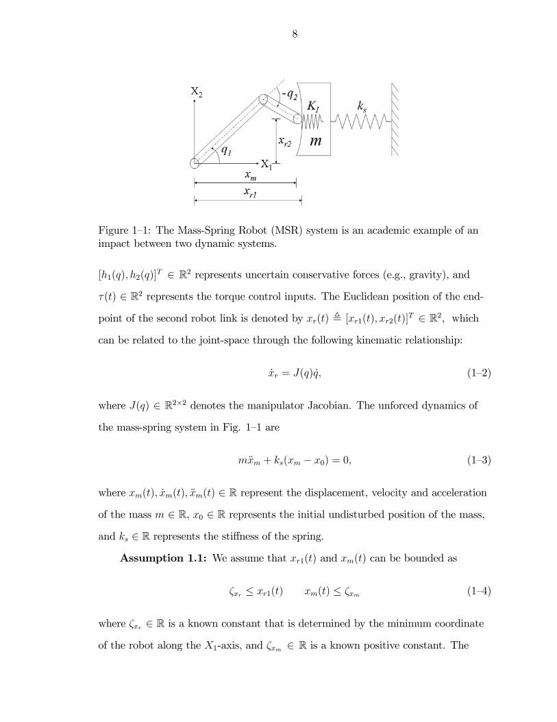
The subsequent development is motivated by the academic problem illustrated

in Fig. 1—1. The dynamic model for the two-link revolute robot depicted in Fig.

1—1 can be expressed in the joint-space as

M(q)q + C(q, q)q + h(q) = τ, (1—1)

where q(t), q(t), q(t) ∈ R2 represent the angular position, velocity, and acceleration

of the robot links, respectively, M(q) ∈ R2×2 represents the uncertain inertia

matrix, C(q, q) ∈ R2×2 represents the uncertain centripetal-Coriolis effects, h(q) ,

8

Figure 1—1: The Mass-Spring Robot (MSR) system is an academic example of animpact between two dynamic systems.

[h1(q), h2(q)]T ∈ R2 represents uncertain conservative forces (e.g., gravity), and

τ(t) ∈ R2 represents the torque control inputs. The Euclidean position of the end-

point of the second robot link is denoted by xr(t) , [xr1(t), xr2(t)]T ∈ R2, which

can be related to the joint-space through the following kinematic relationship:

xr = J(q)q, (1—2)

where J(q) ∈ R2×2 denotes the manipulator Jacobian. The unforced dynamics of

the mass-spring system in Fig. 1—1 are

mxm + ks(xm − x0) = 0, (1—3)

where xm(t), xm(t), xm(t) ∈ R represent the displacement, velocity and acceleration

of the mass m ∈ R, x0 ∈ R represents the initial undisturbed position of the mass,

and ks ∈ R represents the stiffness of the spring.

Assumption 1.1: We assume that xr1(t) and xm(t) can be bounded as

ζxr ≤ xr1(t) xm(t) ≤ ζxm (1—4)

where ζxr ∈ R is a known constant that is determined by the minimum coordinate

of the robot along the X1-axis, and ζxm ∈ R is a known positive constant. The

9

lower bound assumption for xr1(t) is based on the geometry of the robot, and the

upper bound assumption for xm(t) is based on the physical fact that the mass is

attached by the spring to some object, and the mass will not be able to move past

that object.

In the following, the contact model is considered as an elastic contact with

finite stiffness. An impact between the second link of the robot and the spring-mass

system occurs when xr1(t) ≥ xm(t) (see Fig. 1—1). The impact will yield equal and

opposite force reactions between the robot and mass-spring system. Specifically,

the impact force acting on the mass, represented by Fm(xr, xm) ∈ R, is assumed to

have the following form [6], [10]

Fm = KIΛ(xr1 − xm), (1—5)

where KI ∈ R represents a positive stiffness constant, and Λ(xr, xm) ∈ R is defined

as

Λ =

⎧⎪⎨⎪⎩ 1 xr1 ≥ xm

0 xr1 < xm.(1—6)

The impact force acting on the robot links produces a torque, denoted by

τd(xr, xm, q) ∈ R2, as follows:

τd = KIΛ (xr1 − xm)

⎡⎢⎣ l1 sin(q1) + l2 sin(q2 + q1)

l2 sin(q2 + q1)

⎤⎥⎦ , (1—7)

where l1, l2 ∈ R denote the robot link lengths. Based on (1—1), (1—3), and (1—5)-(1—

7), the dynamic model for the MSR system can be expressed as

M(q)q + C(q, q)q + h(q)− τd = τ

mxm + ks(xm − x0) = Fm.(1—8)

10

After premultiplying the robot dynamics by the inverse of the Jacobian

transpose and utilizing (1—2), the dynamics in (1—8) can be rewritten as [13], [14]

M (xr) xr + C (xr, xr) xr + h(xr) +

⎡⎢⎣ Fm

0

⎤⎥⎦ = F (1—9)

mxm + ks(xm − x0) = Fm, (1—10)

where F (t) , J−T (q)τ(t) ∈ R2 denotes the manipulator force. The dynamic model

in (1—9) and (1—10) exhibits the following properties that will be utilized in the

subsequent analysis.

Property 1.1: The inertia matrix M(xr) is symmetric, positive definite, and

can be lower and upper bounded as

a1||ξ||2 ≤ ξTMξ ≤ a2||ξ||2, ∀ξ ∈ R2 (1—11)

where a1, a2 ∈ R are positive constants.

Property 1.2: The following skew-symmetric relationship is satisfied

ξT (1

2

·M(xr)− C(xr, xr))ξ = 0 ∀ξ ∈ R2. (1—12)

CHAPTER 2LYAPUNOV-BASED CONTROL OF A ROBOT AND MASS-SPRING SYSTEM

UNDERGOING AN IMPACT COLLISION

This chapter and our preliminary efforts in [13] provide a first step at con-

trolling the proposed impact system in Section 1.2. The academic example of a

planar robot colliding with an unactuated mass-spring system is used to represent

a broader class of such systems. The control development in this chapter is based

on the assumption of exact model knowledge of the system dynamics. The control

objective is to command a robot to collide with an unactuated mass-spring sys-

tem and regulate the spring-mass to a desired compressed state. Lyapunov-based

methods are used to develop a continuous controller that yields global asymp-

totic regulation of the spring-mass and robot links. Unlike some other results in

literature, the developed continuous force controller does not depend on sensing

the impact, measuring the impact force, or the measurement of other acceleration

terms. Experimental results are provided to validate our analysis.

This chapter is organized as follows. Section 2.1 describes the error system and

control development followed by the stability analysis in Section 2.2. Section 2.3

describes the experimental set up and results that indicate the successful perfor-

mance obtained by implementing the proposed controller followed by conclusion in

Section 2.4.

2.1 Error System and Control Development

2.1.1 Control Objective

One goal in this chapter is to regulate the states of a dynamic system (i.e., a

two-link planar robot) that has an impact collision with another dynamic system

(i.e., a mass-spring). A regulation error, denoted by e(t) ∈ R3, is defined to

11

12

quantify the control objective as

e ,∙eTr em

¸T(2—1)

where er(t) , [er1, er2]T ∈ R2 and em(t) ∈ R denote the regulation error for the

robot and mass-spring system, respectively, and are defined as

er , xrd − xr em , xmd − xm. (2—2)

In (2—2), xmd ∈ R denotes the constant known desired position of the spring-mass.

The desired position of the end-point of the second robot link, denoted by xrd(t)

, [xrd1, xrd2]T ∈ R2, is selected so that the robot will produce the desired spring-

mass position while accounting for the impact dynamics. Specifically, xrd1(t) (i.e.,

the desired horizontal Euclidean coordinate in Fig. 1—1) is a time-varying signal

that is subsequently designed to account for the impact condition and the coupled

dynamic response of the MSR system, and xrd2 (i.e., the desired vertical Euclidean

coordinate in Fig. 1—1) is selected as a constant. Filtered tracking errors, denoted

by rr(t) ∈ R2 and rm(t) ∈ R, are defined as

rr , er + αer rm , em + αem (2—3)

to facilitate the subsequent control design and stability analysis where α ∈ R is a

positive control parameter.

2.1.2 Closed-Loop Error System

By taking the time derivative of mrm(t) and utilizing (2—2) and (2—3), the

following open-loop error system can be obtained:

mrm = k(xm − x0)−KΛ(xr1 − xm) + αmem (2—4)

where the spring-mass dynamics in (1—10) were substituted for mxm(t). Motivated

to design the desired robot link trajectory to position the spring-mass, (2—2) is used

13

to rewrite the open-loop system in (2—4) as

mrm = k(xm − x0) + αmem +KΛer1 +KΛxm −KΛxrd1. (2—5)

Based on (2—5), the desired robot link position is designed as

xrd1 ,1

K(αmem + k(xm − x0)) +

1

K(k1 + k2) rm + xm (2—6)

xrd2 , ε

where ε ∈ R is an appropriate positive constant (i.e., ε is selected so the robot will

impact the mass-spring system), and k1 and k2 ∈ R are positive constant control

gains. After substituting (2—6) into (2—5), the closed-loop error system for rm(t)

can be obtained as

mrm = (1− Λ) (k(xm − x0) + αmem) +KΛer1 − Λ (k1 + k2) rm. (2—7)

As xm(t) → xmd, (2—2) and (2—3) can be used to conclude that rm(t) → 0,

em(t)→ 0, and em(t)→ 0. Hence, (2—6) can be used to conclude that

xrd1(t)→k

K(xm − x0) + xmd. (2—8)

The physical meaning of (2—8) is that the desired robot position varies in time to

account for the impact dynamics and the coupled dynamic system, and the desired

steady-state value is a constant that equals the desired spring-mass position plus

the mass deformation.

After taking the time derivative of rr(t) and premultiplying by the robot

inertia matrix, the following open-loop error system is obtained:

Mrr = Mxrd − F + Cxr + h+

⎡⎢⎣ KΛ(xr1 − xm)

0

⎤⎥⎦+ αMer, (2—9)

14

where (1—10) and (2—2) were utilized. Based on (2—9) and the subsequent stability

analysis, the robot force control input is designed as

F , Mxrd + Cxrd + h+

⎡⎢⎣ KΛ(xr1 − xm)

0

⎤⎥⎦+ k3rr + α¡Mer + Cer

¢+ er, (2—10)

where k3 ∈ R is a positive constant control gain. Based on the use of the backstep-

ping method, the robot force control input in (2—10) requires the first and second

derivative of xrd(t). As described in the Appendix A, the first and second derivative

of xrd(t) exists (i.e., xrd(t) is continuously differentiable) and do not depend on

acceleration terms. The closed-loop error system for rr(t) can be obtained after

substituting (2—10) into (2—9) as

Mrr = −k3rr − Crr − er. (2—11)

2.2 Stability Analysis

Theorem: The controller given by (2—10) ensures global asymptotic stability of

the robot and spring-mass regulation errors in the sense that

|em(t)|→ 0 ker(t)k→ 0 as t→∞ (2—12)

provided the following gain condition is satisfied:

α >K2

4k2. (2—13)

In the following proof, a Lyapunov function and its derivative are provided.

The analysis is then separated into two cases: contact and non-contact. For the

non-contact case, the stability analysis indicates the controller and error signals are

bounded and converge to an arbitrarily small region. Additional analysis indicates

that within this region, contact must occur. When contact occurs, a Lyapunov

15

analysis is provided that illustrates the MSR system asymptotically converges to

the desired setpoint.

Proof: Let V (rm, rr, er) ∈ R denote the following continuously differentiable,

nonnegative, radially unbounded function (i.e. a Lyapunov function candidate)

V , 1

2mr2m +

1

2rTr Mrr +

1

2eTr er. (2—14)

The Lyapunov function candidate in (2—14) can be lower and upper bounded as

γ1 kzk2 ≤ V ≤ γ2 kzk2 (2—15)

where γ1, γ2 ∈ R are positive constants, and z(t) ∈ R5 is defined as

z(t) ,∙rm rTr eTr

¸T.

The time derivative of (2—14) can be determined as

V = rTm((1− Λ) (k(xm − x0) + αmem)) + rTmKΛer1 (2—16)

− Λ (k1 + k2) rTmrm − k3r

Tr rr − αeTr er

where (1—12), (2—3), (2—7), and (2—11) were utilized. The remainder of the analysis

is divided into two cases: Case 1-the robot and mass-spring systems are not in

contact (i.e., xr1 < xm and Λ = 0), and Case 2-the robot and mass-spring systems

are in contact (i.e., xr1 ≥ xm and Λ = 1).

Case 1a: Before the initial contact, the mass-spring system is at rest and the

spring is not compressed; hence,

k(xm − x0) = 0 em = 0. (2—17)

Based on (2—17), (2—16) can be expressed as

V = −k3rTr rr − αeTr er. (2—18)

16

The expressions in (2—14) and (2—18) can be used to prove that er(t), rr(t),

rm(t) ∈ L∞ and that er(t), rr(t) ∈ L2. Based on the fact that er(t), rr(t),

rm(t) ∈ L∞, standard signal chasing arguments can be used to prove that er(t),

rr(t), xrd(t), F (t) ∈ L∞ along with all of the other closed-loop signals. Since er(t),

rr(t) ∈ L∞ ∩ L2 and are uniformly continuous, Barbalat’s Lemma can be applied to

conclude that

krr(t)k→ 0 ker(t)k→ 0 as t→∞. (2—19)

The result in (2—19) can be used along with (2—6) to conclude that

xrd1(t)→1

K(k1 + k2)αem + x0

leading to an impact with the mass-spring system.

Case 1b: After an impact, the robot may loose contact with the spring-mass.

In this case

k(xm − x0) 6= 0 em = −xm. (2—20)

Based on (2—20), (2—16) can be expressed as

V = rTm (k(xm − x0) + αmem + rm)− k3rTr rr − αeTr er − rTmrm. (2—21)

For this case, the initial velocity of the spring-mass is denoted by ξ ∈ R and the

initial position is denoted by xm ∈ R. Given the aforementioned initial conditions,

the solution for xm(t) can be obtained from (1—10) as

xm(t) = x0 + (xm − x0) cos(

rk

mt) + ξ

rm

ksin(

rk

mt). (2—22)

The time derivative of (2—22) can be expressed as

xm(t) = − (xm − x0)

rk

msin(

rk

mt) + ξ cos(

rk

mt). (2—23)

17

Based on (2—22) and (2—23), rm(t) can be expressed as follows:

rm = (xm − x0)

rk

msin(

rk

mt)− ξ cos(

rk

mt) + αxmd − αxm(t). (2—24)

The expressions in (2—22)-(2—24) can be upper bounded as

|xm| ≤ |x0|+ |xm − x0|+ |ξ|r

m

k≤ ζ1 (2—25)

|xm| ≤ |xm − x0|¯¯r

k

m

¯¯+ |ξ| ≤ ζ2 (2—26)

|rm| ≤ |xm − x0|¯¯r

k

m

¯¯+ |ξ|+ α (xmd + ζ1) ≤ ζ3 (2—27)

where ζ1, ζ2, ζ3 ∈ R denote positive constants. After utilizing (2—25)-(2—27), an

upper bound for (2—21) can be developed as

V ≤ −βV + δ (2—28)

where δ ∈ R is a positive constant, and β ∈ R is defined as

β , min(k3, α, 1)

γ2.

Standard techniques can be used to solve (2—28) for V (t) as

V (t) ≤µV (0)− δ

β

¶exp(−βt) + δ

β. (2—29)

Based on (2—29), it is clear that during the transient case (Case 1b) that er(t),

rr(t), rm(t) ∈ L∞. Based on the fact that er(t), rr(t), rm(t) ∈ L∞, standard signal

chasing arguments can be used to prove that er(t), rr(t), xrd(t), F (t) ∈ L∞ along

with all of the other closed-loop signals.

As V (t) → 0, eventually βV ≤ δ. The previous development can be used to

conclude that for the non-contact case

V → δ

βand hence, krr(t)k , ker(t)k , |rm(t)|→

δ

βas t→∞. (2—30)

18

Further analysis is required to prove that the manipulator makes contact with

the mass-spring system and to achieve the control objective. Contact between the

manipulator and the mass-spring system occurs when xr1(t) ≥ xm(t). Based on

(2—30), a sufficient condition for contact can be developed as

xrd1 ≥ xm +δ

β. (2—31)

After using (2—6), the sufficient condition in (2—31) can be expressed as

1

K(αmem + k(xm − x0)) +

1

K(k1 + k2) rm ≥

δ

β. (2—32)

By using (1—4), (2—3), and (2—30), the inequality in (2—32) can be expressed as

1

K(αm(

δ

β− α(xmd − ζxm)) + k(ζxm − x0)) +

1

K(k1 + k2)

δ

β≥ δ

β. (2—33)

Based on (2—33), the control parameter k1 and k2 can be selected according to the

following sufficient condition to ensure the robot and mass-spring system make

contact

k1 + k2 ≥ K − αm+α2βm

δ(xmd − ζxm) +

αβkm

δ(ζxm − x0). (2—34)

Case 2: When the robot and mass-spring systems are in contact, (2—16) can

be upper bounded as

V ≤ −k1 krmk2 − k3 krrk2 − α kerk2 + [K krmk kerk− k2 krmk2]. (2—35)

After completing the squares on the bracketed terms, the following expression is

obtained:

V ≤ −k1 krmk2 − k3 krrk2 −µα− K2

4k2

¶kerk2 . (2—36)

Provided the gain condition given in (2—13) is satisfied, (2—15) can be used to

upper bound (2—36) as

V ≤ −γ3V (2—37)

19

where γ3 ∈ R is a positive constant. The expression in (2—37) indicates that while

in contact, the robot and spring-mass position errors are exponentially regulated,

and er(t), rr(t), rm(t) ∈ L∞. Based on the fact that er(t), rr(t), rm(t) ∈ L∞,

standard signal chasing arguments can be used to prove that er(t), rr(t), xrd(t),

F (t) ∈ L∞ along with all of the other closed-loop signals.

2.3 Experimental Results

The testbed depicted in Fig. 2—1 and Fig. 2—2 was developed for experimental

demonstration of the proposed controller. The testbed is composed of a mass-

spring system and a two-link robot. The body of the mass-spring system includes

a U-shaped aluminum plate (item (8) in Fig. 2—1) mounted on an undercarriage

with porous carbon air bearings which enables the undercarriage to glide on an

air cushion over a glass covered aluminum rail. A steel core spring (item (1) in

Fig. 2—1) connects the undercarriage to an aluminum frame, and a linear variable

displacement transducer (LVDT) (item (2) in Fig. 2—1) is used to measure the

position of the undercarriage assembly. The impact surface consists of an aluminum

plate connected to the undercarriage assembly through a stiff spring mechanism

(item (7) in Fig. 2—1). A capacitance probe (item (3) in Fig. 2—1) is used to

measure the deflection of the stiff spring mechanism. The two-link robot (items

(4-6) in Fig. 2—1) is made of two aluminum links, mounted on 240.0 Nm (base

link) and 20.0 Nm (second link) direct-drive switched reluctance motors. The

motors are controlled through power electronics operating in torque control mode.

The motor resolvers provide rotor position measurements with a resolution of

614400 pulses/revolution, and a standard backwards difference algorithm is used

to numerically determine velocity from the encoder readings. A Pentium 2.8 GHz

PC operating under QNX hosts the control algorithm, which was implemented

via Qmotor 3.0, a graphical user-interface, to facilitate real-time graphing, data

logging, and the ability to adjust control gains without recompiling the program

20

Figure 2—1: Top view of experimental testbed including: (1) mass-spring, (2)LVDT, (3) capacitance probe, (4) link 1, (5) motor 1, (6) link 2, (7) stiff springmechanism, (8) mass.

Figure 2—2: Side view of experimental testbed

(for further information on Qmotor 3.0, the reader is referred to [44]). Data

acquisition and control implementation were performed at a frequency of 2.0 kHz

using the ServoToGo I/O board.

21

The parameters for the dynamic model in (1—9) and (1—10) have the following

values:

m1 = 7.10 [kg] m2 = 1.11 [kg]

m = 13.6 [kg] ms = 10.0 [kg]

l1 = 0.37 [m] l2 = 0.17 [m]

k = 2000 [N/m] K = 1.8× 106 [N/m] ,

where m1, m2 ∈ R represent the mass of the first and second link, m ∈ R

is the mass of the cart, and ms ∈ R is the mass of the motor that drives the

second link. The control gains α and k3, defined as scalars in (2—3) and (2—10),

were implemented (with nonconsequential implications to the stability result) as

diagonal gain matrices to provide more flexibility in the experiment. Specifically,

the control gains were selected as

k1 = 1 k2 = 10000 k3 = diag {250, 12} α = diag {95, 100, 90} .

The initial conditions for the robot coordinates and the spring-mass position were

(in [m]) ∙xr1(0) xr2(0) xm(0)

¸=

∙0.016 0.487 0.203

¸.

The initial velocity of the robot and spring-mass were zero, and the desired spring-

mass position was (in [mm])

xmd = 233.

That is, the tip of the second link of the robot was initially 217 mm from the

desired setpoint and 187 mm from impact along the X1-axis (see Fig. 2—1).

Therefore, once the initial impact occurs, the robot is required to depress the

spring (item (1) in Fig. 2—1) to move the mass 30 mm along the X1-axis.

22

The mass-spring and robot errors (i.e., e(t)) are shown in Fig. 2—3. The peak

steady-state position error of the robot tip along the X1-axis (i.e., |er1|) and along

the X2-axis (i.e., |er2|) are 9.6 μm and 92 μm, respectively. The peak steady-state

position error of the spring-mass (i.e., |em|) is 7.7 μm. The 92 μm is due to the lack

of the ability of the model to capture friction and slipping effects on the contact

surface. In this experiment, a significant friction effect is present along the X2-axis

between the robot tip and the contact surface due to a large normal spring force

that is applied along the X1-axis.

The input control torques (i.e., JT (q)F (t)) are shown in Fig. 2—4 and Fig.

2—5. To constrain the impact force to a level that ensured the aluminum plate did

not flex to the point of contact with the capacitance probe, the computed torques

are artificially saturated. Fig. 2—4 depicts the computed torques, and Fig. 2—5

depicts the actual torques (solid line) along with the computed torques (dashed

line). The resulting desired trajectory along the X1-axis (i.e., xrd1(t)) is depicted

in Fig. 2—6, and the desired trajectory along the X2-axis was chosen as xrd2 = 368

mm. Fig. 2—7 depicts the value of Λ(xr, xm) that indicates contact (Λ = 1) and

non-contact (Λ = 0) conditions for the robot and mass-spring system. A video of

the experiment is provided in [45].

23

0 0.5 1 1.5 2 2.5 3 3.5 4−500

0

500(a)

[mm

]

0 0.5 1 1.5 2 2.5 3 3.5 4−200

0

200(b)

[mm

]

0 0.5 1 1.5 2 2.5 3 3.5 4−20

0

20

40(c)

[sec]

[mm

]

Figure 2—3: The spring-mass and robot errors e(t). Plot (a) indicates the positionerror of the robot tip along the X1-axis (i.e., er1(t)), (b) indicates the position errorof the robot tip along the X2-axis (i.e., er2(t)), and (c) indicates the position errorof the spring-mass (i.e., em(t)).

0 0.5 1 1.5 2 2.5 3 3.5 4−3000

−2000

−1000

0

1000(a)

[Nm

]

0 0.5 1 1.5 2 2.5 3 3.5 4−100

−50

0

50(b)

[sec]

[Nm

]

Figure 2—4: Computed control torques JT (q)F (t) for the (a) base motor and (b)second link motor.

24

0 0.2 0.4 0.6 0.8 1 1.2−300

−200

−100

0

100

200

(a)

[Nm

]

0 0.2 0.4 0.6 0.8 1 1.2−8

−6

−4

−2

0

2

4(b)

[sec]

[Nm

]

Figure 2—5: Applied control torques JT (q)F (t) (solid line) versus computed controltorques (dashed line) for the (a) base motor and (b) second link motor.

0 0.5 1 1.5 2 2.5 3 3.5 4215

220

225

230

235

240

[sec]

[mm

]

Figure 2—6: Computed desired robot trajectory, xrd1(t).

25

0 0.5 1 1.5 2 2.5 3 3.5 4−0.2

0

0.2

0.4

0.6

0.8

1

[sec]

Figure 2—7: Contact (Λ = 1) and non-contact (Λ = 0) conditions for the robot andmass-spring system.

2.4 Concluding Remarks

A nonlinear Lyapunov-based controller is proven to regulate the states of a

planar robot colliding with an unactuated mass-spring system. The continuous

controller yields global asymptotic regulation of the spring-mass and robot links.

Unlike some other results in literature, the developed continuous force controller

does not depend on sensing the impact, measuring the impact force, or the mea-

surement of other acceleration terms. Innovative analysis methods are used to

prove the stability of the system during contact and during different noncontact

states. Experimental results are provided to illustrate the successful controller

performance.

CHAPTER 3GLOBAL ADAPTIVE LYAPUNOV-BASED CONTROL OF A ROBOT AND

MASS-SPRING SYSTEM UNDERGOING AN IMPACT COLLISION

Similar to Chapter 2, this chapter and our preliminary results in [14] consider

a fully actuated planar robot colliding with an unactuated mass-spring system,

but unlike Chapter 2 the dynamic model for both the mass-spring and robot

systems and the impact force are assumed to have uncertain parameters. The

control objective is also defined as the desire to command the robot to collide

with an unactuated system and regulate the resulting coupled MSR system to a

desired compressed state while compensating for the constant, unknown system

parameters. Specifically, in the dynamic model of Section 1.2, M(q) ∈ R2×2

represents the uncertain inertia matrix, C(q, q) ∈ R2×2 represents the uncertain

centripetal-Coriolis effects, and h(q) , [h1(q), h2(q)]T ∈ R2 represents uncertain

conservative forces (e.g., gravity), m ∈ R represents the unknown mass and ks ∈ R

represents the unknown stiffness of the spring, and KI ∈ R represents the unknown

positive stiffness constant.

To compensate for the uncertainty, adaptive Lyapunov-based methods are used

to develop a continuous adaptive controller that yields global asymptotic regulation

of the mass and robot links. Two linear parameterizations are designed to adapt

for the unknown robot and mass parameters. A desired time-varying robot link

trajectory is designed that accounts for the impact dynamics and the resulting

coupled dynamics of the MSR system. The desired link trajectory converges to a

setpoint that equals the desired mass position plus an additional constant that is

due to the deformation of the mass. A force controller is then designed to ensure

that the robot link position tracking error is regulated.

26

27

This chapter is organized as follows. The associated properties and assump-

tions are provided in Section 3.1. Section 3.2 describes the error system and control

development followed by the stability analysis in Section 3.3. Section 3.4 describes

the experimental results that indicate the successful performance of the proposed

controller followed by conclusion in Section 3.5.

3.1 Properties and Assumptions

Property 3.1: The robot dynamics given in (1—9) can be linearly parameter-

ized as

Y (xr, xr, xr)θ = M (xr) xr + C (xr, xr) xr + h(xr) +

⎡⎢⎣ Fm

0

⎤⎥⎦ ,where θ ∈ Rp contains the constant unknown system parameters, and Y (xr, xr,

xr) ∈ R2×p denotes the known regression matrix.

Assumption 3.1: We assume that the mass of the mass-spring system can be

upper and lower bounded as

ml < m < mu

where ml,mu ∈ R denote known positive bounding constants. The unknown

stiffness constants KI and ks are also assumed to be bounded as

ζK< KI < ζK ζ

ks< ks < ζks (3—1)

where ζK, ζK , ζks

, ζks ∈ R denote known positive bounding constants.

Assumption 3.2: During the subsequent control development, we assume

that the minimum singular value of J(q) is greater than a known, small positive

constant δ > 0, such that max {kJ−1(q)k} is known a priori, and hence, all

kinematic singularities are always avoided.

28


The subsequent control design is based on integrator backstepping methods. A

desired trajectory is designed for the robot (i.e., a virtual control input) to ensure

the robot converges to and impacts with the mass, and to ensure that the robot

regulates the mass to the desired position. Since we can not directly control the

robot trajectory, a force controller is developed to ensure that the robot tracks the

desired trajectory despite the transition from free motion to an impact collision and

despite uncertainties throughout the MSR system. As is typical of the backstepping

design method, the derivative of the desired robot trajectory is required to develop

the force controller. Taking the derivative of the desired trajectory could lead to

unmeasurable higher order terms (i.e., acceleration). The subsequent development

exploits the hyperbolic filter structure developed in [42] to overcome the problem of

injecting higher order terms in the controller and to facilitate the development of

sufficient gain conditions used in the subsequent stability analysis.


The control objective is to regulate the states of an uncertain dynamic system

(i.e., a two-link planar robot) that has an impact collision with another uncertain

dynamic system (i.e., a mass-spring). A regulation error, denoted by e(t) ∈ R3, is

defined to quantify this objective as

e ,∙em eTr

¸T,

where er(t) , [er1, er2]T ∈ R2 and em(t) ∈ R denote the regulation error for the

end-point of the second link of the robot and mass-spring system (see Fig. 1—1),

respectively, and are defined as


29

In (3—2), xmd ∈ R denotes the constant known desired position of the mass, and

xrd(t) , [xrd1(t), xrd2]T ∈ R2 denotes the desired position of the end-point of the

second link of the robot. The subsequent development is based on the assumption

that q(t), q(t), xm(t), and xm(t) are measurable, and that xr(t) and xr(t) can

be obtained from q(t) and q(t). To facilitate the subsequent control design and

stability analysis, filtered tracking errors, denoted by ηm(t) ∈ R and rr(t) ∈ R2, are

defined as [42]

ηm , em + α1 tanh(em) + α2 tanh(ef) (3—3)

rr , er + αer,

where α, α1, α2 ∈ R are positive, constant gains, and ef(t) ∈ R is an auxiliary filter

variable designed as [42]

ef , −α3 tanh(ef) + α2 tanh(em)− k1 cosh2(ef)ηm, (3—4)

where k1 ∈ R is a positive constant control gain, and α3 ∈ R is a positive constant

filter gain.


By taking the time derivative of mηm(t) and utilizing (1—5), (1—10), (3—2), and

(3—3), the following open-loop error system can be obtained:

mηm = Ydθd −KIΛ (xr1 − xm) + α2m cosh−2(ef)ef + α1m cosh

−2(em)em. (3—5)

In (3—5), Yd(xm) , (xm − xo) and θd , ks. To facilitate the subsequent analysis, the

following notation is introduced [42]:

Ydθd = YdKIK−1I θd = Ydkθdk (3—6)

= KI (xm − xo)

∙ksKI

¸.

30

After using (3—3) and (3—4), the expression in (3—5) can be rewritten as

mηm = Ydθd +KI (xrd1 − Λxr1) +KIΛxm −KIxrd1 + χ− α2mk1ηm, (3—7)

where χ(em, ef , ηm, t) ∈ R is an auxiliary term defined as

χ = α1m cosh−2(em) (ηm − α1 tanh(em))− α1α2m cosh

−2(em) tanh(ef) (3—8)

+ α2m cosh−2(ef) (−α3 tanh(ef)) + α2m cosh

−2(ef) (α2 tanh(em)) .

The auxiliary expression χ(em, ef , ηm, t) defined in (3—8) can be upper bounded as

|χ| ≤ ζ1 kzk , (3—9)

where ζ1 ∈ R is a positive bounding constant, and z(t) ∈ R3 is defined as

z =

∙ηm tanh(em) tanh(ef)

¸. (3—10)

Based on (3—7) and the subsequent stability analysis, the desired robot link

position is designed as

xrd1 , Ydθdk + xm + k2 tanh(em)− k1k2 cosh2(ef) tanh(ef) (3—11)

xrd2 , ε.

In (3—11), ε ∈ R is an appropriate positive constant (i.e., ε is selected so the robot

will impact the mass-spring system in the vertical direction), k2 ∈ R is a positive

constant control gain, and the control gain k1 ∈ R is defined as

k1 ,1

ml

¡3 + kn1ζ

21

¢, (3—12)

where kn1 ∈ R is a positive constant nonlinear damping gain. The parameter

estimate θdk(t) ∈ R in (3—11) is generated by the adaptive update law

·θdk , proj(ΓYdηm). (3—13)

31

In (3—13), Γ ∈ R is a positive constant, and proj(·) denotes a sufficiently smooth

projection algorithm [43] utilized to guarantee that θdk(t) can be bounded as

θdk ≤ θdk ≤ θdk, (3—14)

where θdk, θdk ∈ R denote known, constant lower and upper bounds for θdk(t),

respectively.

After substituting (3—11) into (3—7), the closed-loop error system for ηm(t) can

be obtained as

mηm = KI (xrd1 − Λxr1) +KI (Λxm − xm) +KIk1k2 cosh2(ef) tanh(ef) (3—15)

+ Ydkθdk −KIk2 tanh(em) + χ− α2mk1ηm.

In (3—15), the parameter estimation error θdk(t) ∈ R is defined as

θdk , θdk − θdk.

The open-loop robot error system can be obtained by taking the time deriva-

tive of rr(t) and premultiplying by the robot inertia matrix as

Mrr = Yrθr − Crr − F, (3—16)

where (1—9), (3—2), and (3—3) were utilized, and

Yrθr = Mxrd + αMer + h+ Cxrd + αCxrd +

⎡⎢⎣ KIΛ(xr1 − xm)

0

⎤⎥⎦− αCxr, (3—17)

where Yr(xr, xr, xm, xm, ef , ηm, t) ∈ R2×P denotes a known regression matrix, and θr

∈ RPdenotes an unknown constant parameter vector. See Appendix A for a linearly

parameterizable expression for M (xr) xrd(t) that does not depend on acceleration

terms. Based on (3—16) and the subsequent stability analysis, the robot force

32

control input is designed as

F , Yrθr + er + k3rr, (3—18)

where k3 ∈ R is a positive constant control gain, and θr(t) ∈ RP is an estimate for

θr generated by the following adaptive update law

·θr , proj(ΓrY

Tr rr). (3—19)

In (3—19), Γr ∈ RP×P is a positive definite, constant, diagonal, adaptation gain

matrix, and proj(·) denotes a projection algorithm utilized to guarantee that the

i− th element of θr(t) can be bounded as

θri ≤ θri ≤ θri,

where θri, θri ∈ R denote known, constant lower and upper bounds for each element

of θr(t), respectively.

The closed-loop error system for rr(t) can be obtained after substituting (3—18)

into (3—16) as

Mrr = Yrθr − k3rr − Crr − er. (3—20)

In (3—20), the parameter estimation error θr(t) ∈ RP is defined as

θr , θr − θr. (3—21)

Remark 3.1: Based on (3—18), the control torque input can be expressed as

τ = JT³Yrθr + er + k3rr

´(3—22)

where J(q) denotes the manipulator Jacobian introduced in (1—2).

33


Theorem: The controller given by (3—11), (3—13), (3—18), and (3—19) ensures

global asymptotic regulation of the MSR system in the sense that

|em(t)|→ 0 ker(t)k→ 0 as t→∞

provided k1, k2, and kn1 are selected sufficiently large and the following sufficient

gain condition is satisfied:

α2 > max

½1

α, (ζxm + |ζxr |)2

¾ζ2

K

4(3—23)

where ζxm, ζxr , ζK , and α are defined in (1—4) and (3—1), respectively.

In the following proof, a Lyapunov function and its derivative are provided.

The analysis is then separated into two cases as in Chapter 2. For the non-contact

case, the stability analysis indicates the controller and error signals are bounded

and converge to an arbitrarily small region. Additional analysis indicates that

within this region, contact must occur. When contact occurs, a Lyapunov analysis

is provided that illustrates the MSR system asymptotically converges to the desired

setpoint.

Proof: Let V (rr, er, em, ef , ηm, θr, θdk, t) ∈ R denote the following nonnegative,

radially unbounded function (i.e. a Lyapunov function candidate):

V , 1

2rTr Mrr +

1

2θTr Γ

−1r θr +

1

2θTdkKIΓ

−1θdk (3—24)

+ k2KI [ln (cosh(em)) + ln (cosh (ef))] +1

2eTr er +

1

2mη2m.

The time derivative of (3—24) can be determined as

V = rTr Mrr +1

2rTr

·Mrr + θTr Γ

−1r

·θr + θTdkKIΓ

−1·θdk (3—25)

+ k2KI [tanh(em)em + tanh(ef)ef ] + eTr er + ηmmηm.

34

After using (1—12), (3—3), (3—4), (3—12), (3—13), (3—15), and (3—19)-(3—21), the

expression in (3—25) can be rewritten as

V ≤ −k3rTr rr − α1k2KI tanh2(em)− 3α2η2m − k2KIα3 tanh

2(ef) (3—26)

− kn1ζ21α2η

2m − αeTr er + ηm [KI (xrd1 − Λxr1) +KI (Λxm − xm) + χ] .

The expression in (3—26) will now be examined under two different scenarios.

Case 1-Non-contact: For this case, the systems are not in contact (Λ = 0)

and (3—26) can be rewritten as

V ≤ −k3rTr rr − α1k2KI tanh2(em)− k2KIα3 tanh

2(ef)− 3α2η2m

− kn1ζ21α2η

2m − αeTr er + ηm [KIxrd1 −KIxm + χ] .

Rewriting xrd1(t) and substituting for χ(em, ef , ηm, t) yields


2(ef)− 2α2η2m (3—27)

−£α kerk2 − ζK |ηm| kerk

¤−£kn1α2ζ

21η2m − ζ1 kzk |ηm|

¤−£α2η

2m − ζK |ηm| |xm − xr1|

¤.

After completing the square on the bracketed terms, (3—27) can be expressed as


2(ef)− α2η2m (3—28)

−Ãα2 −

ζ2

K

4α

!η2m +

kzk2

4α2kn1+

ζ2

K (xm − xr1)2

4α2.

Provided kn1 is selected according to the sufficient condition

kn1 >1

4α2minnα1k2ζK , k2ζKα3, α2

o ,the expression in (3—28) can be further reduced as

V ≤ −λ1 kzk2 − k3 krrk2 −Ãα2 −

ζ2

K

4α

!η2m +

ζ2

K (xm − xr1)2

4α2, (3—29)

35

where λ1 ∈ R is defined as

λ1 = minnα1k2ζK, k2ζKα3, α2

o− 1

4α2kn1.

Based on (1—4) in Assumption 1.1, for the non-contact case

ζxr ≤ xr1 ≤ xm ≤ ζxm . (3—30)

Hence, the expression in (3—29) can be upper bounded as

V ≤ −λ kyk2 + εx (3—31)

where λ ∈ R is defined as

λ = min

(λ1, k3,

Ãα2 −

ζ2

K

4α

!),

and y(t) ∈ R5 and εx ∈ R are defined as

y =

∙zT rTr

¸Tεx =

ζ2

K (ζxm + |ζxr |)2

4α2(3—32)

where εx can be made arbitrarily small by making α2 large. Based on (3—24)

and (3—31), either λ kyk2 ≤ εx or λ kyk2 > εx. If λ kyk2 > εx, then Barbalat’s

Lemma can be used to conclude that V (t) → 0 since V (t) is lower bounded, V (t)

is negative semi-definite, and V (t) can be shown to be uniformly continuous. As

V (t)→ 0, eventually λ kyk2 ≤ εx. Provided the sufficient gain condition in (3—23) is

satisfied (i.e., εx < 1), then (3—10), (3—32), and the facts that θr(t) and θdk(t) ∈ L∞

from the use of a projection algorithm, can be used to conclude that V (·) ∈ L∞;

hence, ky(t)k, kz(t)k, krr(t)k, ker(t)k, ηm(t), ef(t), em(t) ∈ L∞. Signal chasing

arguments can be used to prove the remaining closed-loop signals are also bounded

during the non-contact case. The previous development can be used to conclude

36

that for the non-contact case

ky(t)k→r

εxλand hence, krr(t)k→

rεxλas t→∞. (3—33)

Based on (3—33), linear analysis methods (see Lemma A.19 of [41]) can be applied

to (3—3) to prove that

ker(t)k→ ker(0)k exp(−αt) +1

α

rεxλ(1− exp(−αt)) (3—34)

as t→∞ for the non-contact case.

Further analysis is required to prove that the manipulator makes contact with

the mass-spring system and to achieve the control objective. Contact between the

manipulator and the mass-spring system occurs when xr1(t) ≥ xm(t). Based on

(3—34), a sufficient condition for contact can be developed as

xrd1 ≥ xm +1

α

rεxλ. (3—35)

After using (3—11), the sufficient condition in (3—35) can be expressed as

Ydθdk + k2 tanh(em)− k1k2 cosh2(ef) tanh(ef) ≥

1

α

rεxλ. (3—36)

By using (3—2) and (3—6) and performing some algebraic manipulation, the

inequality in (3—36) can be expressed as

k2 tanh(em)− k1k2 cosh2(ef) ≥

1

α

rεxλ− xmdθdk + (em + x0) θdk (3—37)

where θdk(t) and θdk(t) are defined in (3—14). From Assumption 1.1, em(t) can be

upper bounded as

em ≤ εm (3—38)

where εm ∈ R denotes a known positive constant. If em(t) ≤ 0, then the sufficient

condition in (3—37) may not be satisfied. The condition that em(t) ≤ 0 will only

occur if an impact collision occurs that causes the mass to overshoot the desired

37

position. However, even if an impact occurs and the mass overshoots the desired

position, the dynamics will force the mass position error to return to the initial

condition. That is, em(t)→ xmd − x0 > εm where εm ∈ R denotes a known positive

constant. Based on (3—38) and the fact that em(t) will eventually be lower bounded

by εm in a noncontact condition, the inequality in (3—37) can be simplified as

k2¡tanh(εm)− k1 cosh

2(ef)¢≥ 1

α

rεxλ− xmdθdk + (εm + x0) θdk. (3—39)

To further simplify the inequality in (3—39), an upper bound can be determined

for ef(t). The inequality in (3—33) along with (3—10) and (3—32) can be used to

conclude that as the manipulator approaches the mass, ef(t) will eventually be

upper bounded as

ef ≤ tanh−1µ1

α

rεxλ

¶≤ εf , (3—40)

where εf ∈ R is a known positive constant. Based on (3—32) and (3—40), the control

parameter k2 can be selected according to the following sufficient condition to

ensure the robot and mass-spring system make contact

k2 ≥1α

pεxλ− xmdθdk + (εm + x0) θdk

tanh(εm)− k1 cosh2(εf)

(3—41)

where k1 is chosen as

k1 <tanh(εm)

cosh2(εf).

Case 2-Contact: Provided the sufficient condition in (3—41) is satisfied, the

robot will eventually make contact with the mass. For the case when the dynamic

systems collide (Λ = 1), and the two dynamic systems become coupled1 , then

1 The dynamic systems can separate after impact, however this case can still beanalyzed under the Non-contact section of the stability analysis.

38

(3—26) can be rewritten as

V ≤ −k3rTr rr − α1k2KI tanh2(em)− 3α2η2m − k2KIα3 tanh

2(ef)


¤−£kn1ζ

21α2η

2m − ζ1 kzk |ηm|

¤,

where (3—9) was substituted for χ(em, ef , ηm, t). Completing the square on the two

bracketed terms yields

V ≤ −k3rTr rr − α1k2ζK tanh2(em)− α3k2ζK tanh

2(ef) (3—42)

− 3α2η2m +ζ2

Kη2m

4α+

kzk2

4α2kn1.

A final bound can be placed on (3—42) as

V ≤ −minnα1k2ζK , α3k2ζK, α2

okzk2 + kzk2

4α2kn1−Ã2α2 −

ζ2

K

4α

!η2m − k3r

Tr rr.

Because (3—24) is non-negative and its derivative is negative semi-definite,

rr(t), θr(t), θdk(t), er(t), em(t), ef(t), and ηm(t) ∈ L∞. Due to the fact that em(t),

ef(t), and ηm(t) ∈ L∞, the expression in (3—3) can be used to conclude that

em(t) ∈ L∞ (and hence, em(t) is uniformly continuous). Due to the fact that

em(t) ∈ L∞, (3—2) can be used to conclude that xm(t) ∈ L∞. Previous facts can

be used to prove that xrd(t) ∈ L∞, and since er(t) ∈ L∞, then xr(t) ∈ L∞. Due

to the fact that ef(t), em(t), ηm(t) ∈ L∞, (3—4) can be used to conclude that

ef(t) ∈ L∞. The expression in (3—5) can be used to conclude that ηm(t) ∈ L∞

(and hence, ηm(t) is uniformly continuous). Given that rr(t), em(t), ef(t), and

ηm(t) ∈ L∞, Yr(·) ∈ L∞. Since θr(t) ∈ L∞, (3—21) can be used to prove that

θr(t) ∈ L∞. The expression in (3—18) can then be used to prove that F (t) ∈ L∞.

The expression in (3—20) can be used to conclude that rr(t) ∈ L∞ (and hence,

rr(t) is uniformly continuous). Due to the fact that em(t), rr(t), ηm(t) ∈ L2 and

uniformly continuous, Barbalat’s Lemma can be used to conclude that |em(t)| ,

krr(t)k , |ηm(t)| → 0 as t → ∞. Based on the fact that krr(t)k → 0 as t → ∞,

39

standard linear analysis methods (see Lemma A.15 of [41]) can then be used to

prove that ker(t)k→ 0 as t→∞.

As is typical in literature, the controller developed in (3—11), (3—13), (3—18),

and (3—19) is based on the underlying assumption that an arbitrarily large (but

finite) control authority is available. A potential disadvantage of the controller

is that the gain conditions developed above and in (3—23) indicate that kn1, k2,

and α2, respectively, should be selected sufficiently large. As demonstrated by the

subsequent experimental results, the gains may be selected much lower in practice

(i.e., the gains conditions are the result of a conservative Lyapunov analysis).

However, the subsequent experimental section also illustrates that even when the

gain conditions are violated, large initial conditions and a high stiffness coefficient

result in a high gain controller that initially saturates the actuators. The control

torque in the experiment was artificially saturated to reduce the magnitude of the

impact to protect a capacitance probe from contact by excessive bending of the

aluminum rod/spring assembly. Research that can limit the required control torque

for systems that undergo an impact collision will be discussed in Chapter 4.


With the testbed in Section 2.3, the control gains α and k3, defined as scalars

in (3—3) and (3—18), were implemented (with nonconsequential implications to

the stability result) as diagonal gain matrices to provide more flexibility in the

experiment. Specifically, the control gains were selected as

k1 = 0.18 k2 = 0.9 k3 = diag {185, 170}

α1 = 45 α2 = 8 α3 = 0.01 α = diag {60, 90} .(3—43)

The control gains in (3—43) were obtained from a trial and error process and may

not satisfy the sufficient gain conditions developed in the theorem proof. The

sufficient gain conditions are the result of a conservative stability analysis and were

40

used as a guide in the tuning process. The subsequent results indicate that the

developed controller can be applied despite the fact that some gain conditions are

not satisfied.

The adaptation gains were selected as

Γ = 90

Γr = diag{4.01× 1012, 1.2× 107, 0.2, 3.3× 1012, (3—44)

6× 106, 0.1, 2.4× 1011, 7× 105, 0.1, 2.35× 1011}.

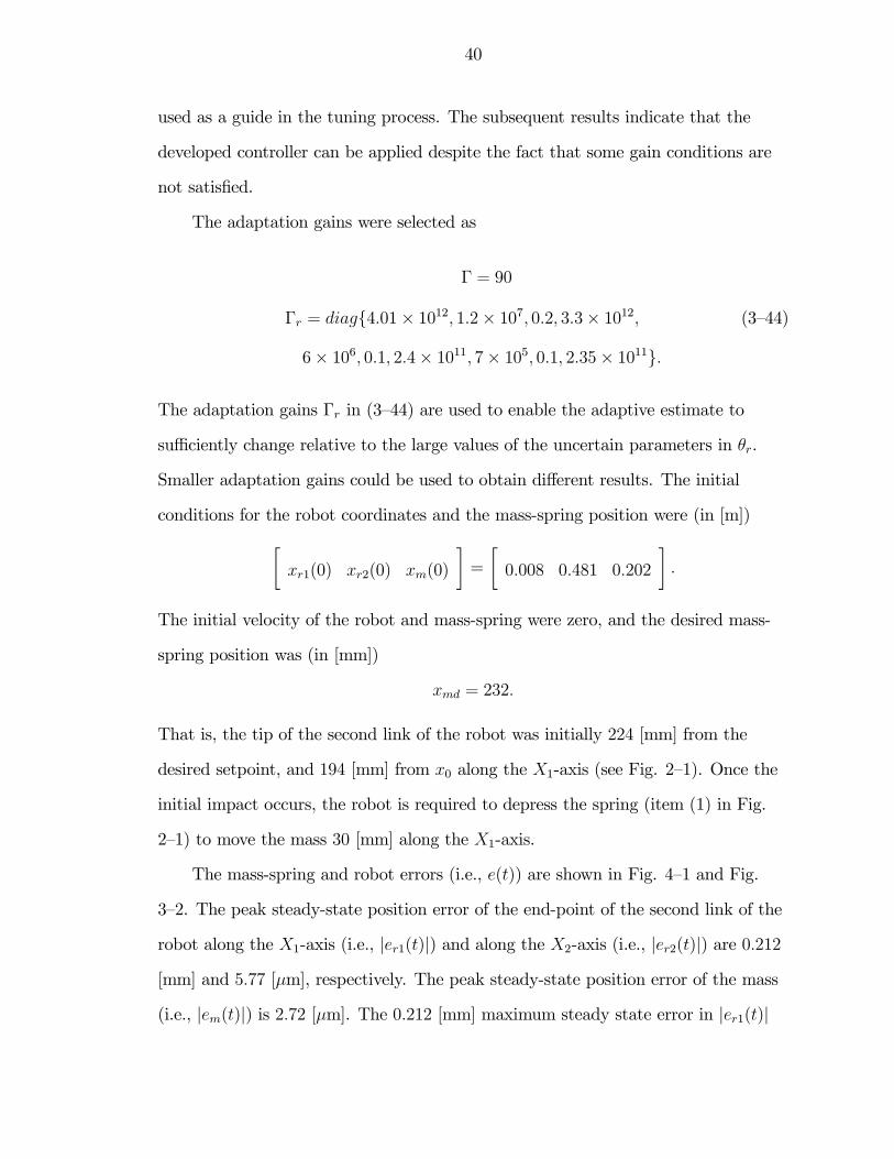
The adaptation gains Γr in (3—44) are used to enable the adaptive estimate to

sufficiently change relative to the large values of the uncertain parameters in θr.

Smaller adaptation gains could be used to obtain different results. The initial

conditions for the robot coordinates and the mass-spring position were (in [m])∙xr1(0) xr2(0) xm(0)

¸=

∙0.008 0.481 0.202

¸.

The initial velocity of the robot and mass-spring were zero, and the desired mass-

spring position was (in [mm])

xmd = 232.

That is, the tip of the second link of the robot was initially 224 [mm] from the

desired setpoint, and 194 [mm] from x0 along the X1-axis (see Fig. 2—1). Once the

initial impact occurs, the robot is required to depress the spring (item (1) in Fig.

2—1) to move the mass 30 [mm] along the X1-axis.

The mass-spring and robot errors (i.e., e(t)) are shown in Fig. 4—1 and Fig.

3—2. The peak steady-state position error of the end-point of the second link of the

robot along the X1-axis (i.e., |er1(t)|) and along the X2-axis (i.e., |er2(t)|) are 0.212

[mm] and 5.77 [μm], respectively. The peak steady-state position error of the mass

(i.e., |em(t)|) is 2.72 [μm]. The 0.212 [mm] maximum steady state error in |er1(t)|

41

0 5 10 15−500

0

500(a)

[mm

]

0 5 10 15−200

0

200(b)

[mm

]

0 5 10 15−50

0

50(c)

[sec]

[mm

]

Figure 3—1: The mass-spring and robot errors e(t). Plot (a) indicates the positionerror of the robot tip along the X1-axis (i.e., er1(t)), (b) indicates the position errorof the robot tip along the X2-axis (i.e., er2(t)), and (c) indicates the position errorof the mass-spring (i.e., em(t)).

is due to the Ydθdk(t) term of xrd1(t) in (3—11) where Yd(xm) is approximately 0.03

[m], and θdk(t) has a maximum steady state value of 0.007 [N/mN/m

], yielding 0.21

[mm] error. All of the other terms in er1(t) are negligible at steady state.

The input control torques in (3—22) are shown in Fig. 3—3 and Fig. 3—4. To

constrain the impact force to a level that ensured the aluminum plate did not

flex to the point of contact with the capacitance probe, the computed torques are

artificially saturated. Fig. 3—3 depicts the computed torques, and Fig. 3—4 depicts

the actual torques (solid line) along with the computed torques (dashed line). The

resulting desired trajectory along the X1-axis (i.e., xrd1(t)) is depicted in Fig. 3—5,

and the desired trajectory along the X2-axis was chosen as xrd2 = 370 [mm]. Fig.

3—6 depicts the value of θdk(t) ∈ R, and Fig. 3—7 - Fig. 3—9 depict the values of

θr(t) ∈ R10. The order of the curves in the plots is based on the relative scale

of the parameter estimates rather than numerical order in θr(t). A video of the

experiment is provided in [46].

42

0 0.5 1 1.5 2

0

100

200

(a)

[mm

]

0 0.5 1 1.5 2−150

−100

−50

0

50(b)

[mm

]

0 0.5 1 1.5 2−20

0

20

40

(c)

[sec]

[mm

]

Figure 3—2: The mass-spring and robot errors e(t) during the initial two seconds.

0 5 10 15−1500

−1000

−500

0

500(a)

[Nm

]

0 5 10 15−600

−400

−200

0

200(b)

[sec]

[Nm

]

Figure 3—3: Computed control torques JT (q)F (t) for the (a) base motor and (b)second link motor.

43

0 0.05 0.1 0.15 0.2 0.25 0.3 0.35 0.4

−100

−50

0

50

(a)

[Nm

]

0 0.05 0.1 0.15 0.2 0.25 0.3 0.35 0.4−100

−50

0

50(b)

[sec]

[Nm

]

Figure 3—4: Applied control torques JT (q)F (t) (solid line) versus computed controltorques (dashed line) for the (a) base motor and (b) second link motor.

0 5 10 15229

229.5

230

230.5

231

231.5

232

232.5

233

233.5

[sec]

[mm

]


44

0 5 10 15−0.01

0

0.01

0.02

0.03

0.04

0.05

0.06

[sec]

Figure 3—6: Unitless parameter estimate θdk(t) introduced in (3—13).

0 5 10 150

0.2

0.4

0.6

0.8

1

1.2

1.4

1.6

1.8

2x 10

6

[sec]

[N/m

]

(a)

(b)

(c)

(d)

Figure 3—7: Estimate for the unknown constant parameter vector θr(t). (a)θr10(t) = KI , (b) θr4(t) = KIms



m, where

m1, m2 ∈ R denote the mass of the first and second link of the robot, ms ∈ Rdenotes the mass of the motor connected to the second link of the robot, and m∈ R denotes the mass of the mass-spring system.

45

0 5 10 150

200

400

600

800

1000

1200

1400

1600

1800

[sec]

[N/m

]

(a)

(b)

(c)

Figure 3—8: Estimate for the unknown constant parameter vector θr(t). (a) θr5(t) =ksms



m.

0 5 10 150

1

2

3

4

5

6

7

8

9

[sec]

[Kg]

(a)

(b)

(c)

Figure 3—9: Estimate for the unknown constant parameter vector θr(t). (a) θr6(t) =ms, (b) θr3(t) = m1, and (c) θr9(t) = m2.

46


An adaptive nonlinear Lyapunov-based controller is proven to regulate the

states of a planar robot colliding with an unactuated mass-spring system. The

continuous controller yields global asymptotic regulation of the spring-mass and

robot links. New control design, error system development and stability analysis

techniques were required to compensate for the fact that the dynamics changed

from an uncoupled state to a coupled state. Experimental results are provided

to illustrate the successful performance of the controller. Sufficient conditions

developed in the stability analysis indicate that the control gains should be selected

large enough to minimize the closed-loop steady state error, but high gains could

result in large torques for large initial errors. The high gain problem is exacerbated

in the developed result because of the presence of the estimated impact stiffness

coefficient. The experimental results were obtained by artificially saturating the

torque to prevent damage to the capacitance probe. These issues point to a need

to develop controllers that account for limited actuation which we will discuss in

Chapter 4.

CHAPTER 4AN IMPACT FORCE LIMITING ADAPTIVE CONTROLLER FOR A ROBOTICSYSTEM UNDERGOING A NON-CONTACT TO CONTACT TRANSITION

Similar to Chapter 2 and 3, the objective of this chapter is also to control

a robot from a non-contact initial condition to a desired (in-contact) position so

that the mass-spring system is regulated to a desired compressed state. When

the controllers in Chapter 2 and Chapter 3 were implemented in the presence of

large initial conditions, violent impacts between the robot and the mass-spring

system resulted. In fact, the controller was artificially saturated (the saturation

effects were not considered in the stability analysis) to reduce the impact forces

so that the mass deflection would not destroy a capacitance probe. These results

provide the motivation for the control development in this chapter. Specifically, the

feedback elements for the continuous controller in Chapter 3 are contained inside

of hyperbolic tangent functions as a means to limit the impact forces resulting

from large initial conditions as the robot transitions from non-contact to contact

states. The main challange of this work is that the use of saturated feedback does

not allow some coupling terms to be canceled in the stability analysis, resulting

in the need to develop state dependent upper bounds that reduce the stability

to a semi-global result. New control development, closed-loop error systems, and

Lyapunov-based stability analysis arguements are used to conclude the result.

Experimental results are provided that successfully demonstrate the control

objective.

This chapter is organized as follows. The associated properties are provided

in Section 4.1. Section 4.2 describes the error system and control development

47

48

followed by the stability analysis in Section 4.3. Section 4.4 describes the experi-

mental results that indicate the successful performance of the proposed controller

followed by conclusion in Section 4.5.

4.1 Properties

Remark 4.1: To aid the subsequent control design and analysis, we define the

vector Tanh(·) ∈ Rn as follows

Tanh(δ) , [tanh(δ1), ..., tanh(δn)]T (4—1)

where δ , [δ1, ..., δn]T ∈ Rn.

Property 4.1: The following inequalities are valid for all ξ = [ξ1, ..., ξn]T ∈ Rn

[1]

||ξ|| ≥ ||Tanh(ξ)||

||ξ||+ 1 ≥ ||ξ||tanh(||ξ||) (4—2)

||ξ||2 ≥nXi=1

ln(cosh(ξi)) ≥ ln(cosh(||ξ||)) (4—3)

ξTTanh(ξ) ≥ TanhT (ξ)Tanh(ξ) = ||Tanh(ξ)||2 (4—4)

≥ tanh2(||ξ||).


The subsequent control design is based on integrator backstepping methods. A

desired trajectory is designed for the robot (i.e., a virtual control input) to ensure

the robot converges to and impacts with the mass, and to ensure that the robot

regulates the mass to the desired position. Since the robot trajectory can not be

controlled directly, a force controller is developed to ensure that the robot tracks

the desired trajectory despite the transition from free motion to an impact collision

and despite uncertainties throughout the MSR system.

49


As in Chapter 2 and 3, the control objective is to regulate the states of the

mass-sping system via a two-link planar robot that transitions from non-contact to

contact with the mass-spring through an impact collision. An additional objective

in this chapter is to limit the impact force to prevent damage to the robot or

the environment (i.e., the mass-spring system). A regulation error, denoted by

e(t) ∈ R3, is defined to quantify this objective as

e ,∙em eTr

¸T,

where er(t) , [er1(t), er2(t)]T ∈ R2 and em(t) ∈ R denote the regulation error for the

end-point of the second link of the robot and mass-spring system (see Fig. 1—1),

respectively, and are defined as


In (4—5), xmd ∈ R denotes the constant known desired position of the mass, and

xrd(t) , [xrd1(t), xrd2]T ∈ R2 denotes the desired position of the end-point of the

second link of the robot. The subsequent development is based on the assumption

that q(t), q(t), xm(t), and xm(t) are measurable, and that xr(t) and xr(t) can

be obtained from q(t) and q(t). To facilitate the subsequent control design and

stability analysis, filtered tracking errors, denoted by ηm(t) ∈ R and rr(t) ∈ R2, are

defined as [42]

ηm , em + α1 tanh(em) + α2 tanh(ef) (4—6)

rr , er + αer,

50

where α, α1, α2 ∈ R are positive, constant gains, and ef(t) ∈ R is an auxiliary filter

variable designed as [42]

ef , −α3 tanh(ef) + α2 tanh(em)− k1 cosh2(ef)ηm, (4—7)

where k1 ∈ R is a positive constant control gain, and α3 ∈ R is a positive constant

filter gain.


In this section, the closed-loop error system for ηm is exactly the same as in

(3-5)-(3-15) in Chapter 3. The open-loop robot error system can be obtained by

taking the time derivative of rr(t) and premultiplying by the robot inertia matrix

as

Mrr = Yrθr − Crr − F, (4—8)

where (1—9), (4—5), and (4—6) were utilized, and

Yrθr , Mxrd + αMer + h+ Cxrd + αCxrd +

⎡⎢⎣ KIΛ(xr1 − xm)

0

⎤⎥⎦− αCxr,

where Yr(xr, xr, xm, xm, ef , ηm, t) ∈ R2×P denotes a known regression matrix, and

θr ∈ RPdenotes an unknown constant parameter vector. By making substitutions

from the dynamic model and the previous error systems, xrd(t) can be expressed

without a dependance on acceleration terms. Based on (4—8) and the subsequent

stability analysis, the robot force control input is designed as

F , Yrθr + Tanh(er) + k3Tanh(rr), (4—9)

where k3 ∈ R is a positive constant control gain, and θr(t) ∈ RP is an estimate for

θr generated by the following adaptive update law

·θr , proj(ΓrY

Tr rr). (4—10)

51

In (4—10), Γr ∈ RP×P is a positive definite, constant, diagonal, adaptation gain

matrix, and proj(·) denotes a projection algorithm utilized to guarantee that the

i− th element of θr(t) can be bounded as

θri ≤ θri ≤ θri, (4—11)

where θri, θri ∈ R denote known, constant lower and upper bounds for each element

of θr(t), respectively.

The closed-loop error system for rr(t) can be obtained after substituting (4—9)

into (4—8) as

Mrr = Yrθr − Crr − Tanh(er)− k3Tanh(rr). (4—12)

In (4—12), the parameter estimation error θr(t) ∈ RP is defined as

θr , θr − θr. (4—13)


Theorem: The controller given by (3—11), (3—13), (4—9), and (4—10) ensures

semi-global asymptotic regulation of the MSR system in the sense that

|em(t)|→ 0 ker(t)k→ 0 as t→∞

provided the following sufficient gain conditions are satisfied:

kn1 >1

4α2minnα1k2ζK , α3k2ζK , α2

o (4—14)

α2 > max

½1

4α,ζ2xmλ

¾ζ2

K (4—15)

k3α >

Ãr2Vua1

+ 1

!2(4—16)

52

where Vu ∈ R is defined as

Vu , max½λ1 kz(0)k2 + ζθ, 5λ1(tanh

−1(

rεxλ))2 + ζθ

¾,

λ ∈ R is a known positive constant, and a1, α, α1, α2, α3, kn1, k2, k3, λ1, ζxm, ζxr ,

ζK, and ζK are defined in (1—4), (1—11), (3—1), (3—11), (3—12), (4—6), (4—7), and

(4—9).

As in the previous chapters, the subsequent analysis is separated into two

cases: contact and non-contact. For the non-contact case, the stability analysis

indicates the controller and error signals are bounded and converge to an arbitrarily

small region where contact must occur. When contact occurs, a Lyapunov analysis

is provided that illustrates the MSR system asymptotically converges to the desired

setpoint.

Proof : Let V (t) ∈ R denote the following non-negative, radially unbounded

function (i.e. a Lyapunov function candidate):

V , 1

2rTr Mrr +

1

2θTr Γ

−1r θr +

1

2θTdkKIΓ

−1θdk + eTr er +1

2mη2m (4—17)

+ k2KI [ln (cosh(em)) + ln (cosh (ef))] + ln(cosh(er1)) + ln(cosh(er2))

where (1—11) and (4—3) can be utilized to bound V (t) as

a12||rr||2 ≤ V ≤ λ1 kzk2 + ζθ (4—18)

where λ1, ζθ ∈ R and z ∈ R7 are defined as

λ1 , max{a22, 3,

mu

2, k2ζK}

ζθ ,1

2ζKζ

2θdk

Γ−1 +1

2λmax{Γ−1r } kζθrk

2

z , [rTr , eTr , ηm, em, ef ]T

(4—19)

where λmax{·} ∈ R denotes the maximum eigenvalue of a matrix, and ζθdk ,kζθrk

are the known upper bounds of θdk(t) and°°°θr(t)°°°, respectively. After using (1—12),

53

(3—12), (3—13), (3—15), (4—4), (4—6), (4—7), (4—10), and (4—12), the time derivative

of (4—17) can be determined as

V ≤ −k3 tanh2(krrk)− α1k2KI tanh2(em)− α3k2KI tanh

2(ef) (4—20)

+ 2eTr rr − 2αeTr er − 3α2η2m − kn1ζ21α2η

2m − α tanh2(kerk)

+ ηm [KI (xrd1 − Λxr1) +KI (Λxm − xm) + χ] .

The expression in (4—20) will now be examined under two different scenarios.

Case 1-Non-contact: For this case, the systems are not in contact (Λ = 0)

and (4—20) can be rewritten as

V ≤ −k3 tanh2(krrk)− α1k2KI tanh2(em)− α3k2KI tanh

2(ef) (4—21)

+ 2eTr rr − 2αeTr er − 3α2η2m − kn1ζ21α2η

2m − α tanh2(kerk)

+ ηm [KIxrd1 −KIxm + χ] .

Based on (3—1), (3—9), and (4—5), the expression in (4—21) can be rewritten as

V ≤ −k3 tanh2(krrk)− α1k2ζK tanh2(em)− α3k2ζK tanh

2(ef) (4—22)

− 2α2η2m − α tanh2(kerk)


¤−£kn1ζ

21α2η


¤−£α2η

2m − ζK |ηm| |xm − xr1|

¤− [α kerk2 − 2 kerk krrk].

After completing the square in the bracketed terms, (4—22) can be expressed as

V ≤ −β kzk2 − α tanh2(kerk)−Ãα2 −

ζ2

K

4α

!η2m (4—23)

+ζ2

K(xm − xr1)2

4α2−Ãk3 −

krrk2

α tanh2(krrk)

!tanh2(krrk)

where β ∈ R is defined as

β = minnα1k2ζK , α3k2ζK, α2

o− 1

4α2kn1> 0

54

provided kn1 is selected according to (4—14). Provided α2 is selected according to

the sufficient condition in (4—15), then (1—4), (4—2), (4—18), and the fact that

ζxr ≤ xr1 < xm ≤ ζxm (4—24)

for the non-contact case, can be used to rewrite (4—23) as

V ≤ −β kzk2 − α tanh2(kerk) + εx (4—25)

−

⎛⎝k3 −1

α

Ãr2V

a1+ 1

!2⎞⎠ tanh2(krrk).In (4—25), εx ∈ R is a known positive arbitrarily small constant that is defined as

εx ,ζ2

Kζ2xm

α2.

Provided the following sufficient condition is satisfied

k3α >

Ãr2V

a1+ 1

!2, (4—26)

the expression in (4—25) can be expressed as

V ≤ −λ kyk2 + εx (4—27)

where λ is a known constant and y ∈ R5 is defined as

y ,∙zT tanh(kerk) tanh(krrk)

¸T. (4—28)

In (4—27), εx can be made arbitrarily small by making α2 large. Based on (4—

17) and (4—27), if λ ky(t)k2 > εx, then Barbalat’s Lemma can be used to conclude

that V (t)→ 0 since V (t) is lower bounded, V (t) is negative semi-definite, and V (t)

can be shown to be uniformly continuous. As V (t) → 0, eventually λ ky(t)k2 ≤ εx.

While λ ky(t)k2 > εx, (4—17), (4—18), and (4—27) can be used to conclude that

55

V (t) ∈ L∞, and the sufficient condition given in (4—26) can be expressed as

k3α >

⎛⎝s2 ¡λ1 kz(0)k2 + ζθ¢

a1+ 1

⎞⎠2

. (4—29)

Provided α2 >ζ2Kζ2xmλ

then eventually λ ky(t)k2 ≤ εx < λ. Based on (3—10) and

(4—28), the fact that λ ky(t)k2 ≤ εx < λ can be used to conclude that em(t), ef(t),

er(t), rr(t), ηm(t) ∈ L∞. Since θr(t) and θdk(t) ∈ L∞ from the use of a projection

algorithm, the previous facts can be used to conclude that V (t) ∈ L∞. Signal

chasing arguments can be used to prove the remaining closed-loop signals are also

bounded during the non-contact case provided (4—26) is satisfied.

If the initial conditions for V (0) are large enough that λ ky(t)k2 > εx, then

the condition in (4—29) is sufficient. However, if the initial conditions for V (0) are

inside the region defined by εx, then V (t) can grow larger until λ ky(t)k2 ≤ εx.

Therefore, further development is required to determine how large V (t) can grow

so that the sufficient condition in (4—26) can be satisfied. When V (0) is inside the

region defined by εx, then

ky(t)k ≤r

εxλ. (4—30)

The expression in (4—30) can be used along with (3—10), (4—19), and (4—28) to

conclude that

kz(t)k ≤√5 tanh−1(

rεxλ). (4—31)

The inequality in (4—31) can be used along with (4—18) and (4—19) to rewrite the

sufficient condition in (4—26) as

k3α >

⎛⎝s2 ¡5λ1(tanh−1(pεxλ))2 + ζθ

¢a1

+ 1

⎞⎠2

. (4—32)

Hence, the final sufficient condition for (4—26) is given by (4—16). That is, provided

kn1, α, α2, and k3 are selected larger than known constants (that depends on the

56

initial conditions of the states) according to (4—14)-(4—16) then the all the states

converge to an arbitrarily small neighborhood. Development has been provided (see

Section 3.3) to prove that contact with the mass-spring system is ensured within

this neighborhood.

Case 2-Contact: For the case when the dynamic systems collide (Λ = 1) and

the two dynamic systems become coupled1 , then (4—20) can be rewritten as

V ≤ −k3 tanh2(krrk)− α1k2ζK tanh2(em)− α3k2ζK tanh

2(ef)

− 3α2η2m − α tanh2(kerk)−£α kerk2 − ζK |ηm| kerk

¤−£kn1ζ

21α2η


¤− [α kerk2 − 2 kerk krrk],

where (3—1) was substituted for KI and (3—9) was substituted for χ(em, ef , ηm, t).

Completing the square on the three bracketed terms yields

V ≤ −β kzk2 − α tanh2(kerk)−Ãα2 −

ζ2

K

4α

!η2m (4—33)

−Ãk3 −

krrk2

α tanh2(krrk)

!tanh2(krrk).

Because (4—17) is non-negative, as long as (4—14)-(4—16) are satisfied, (4—33) is

negative semi-definite, and rr(t), θr(t), θdk(t), er(t), em(t), ef(t), and ηm(t) ∈ L∞.

Due to the fact that em(t), ef(t), and ηm(t) ∈ L∞, the expression in (4—6) can

be used to conclude that em(t) ∈ L∞ (and hence, em(t) is uniformly continuous

(UC)). Due to the fact that em(t) ∈ L∞, xm(t) ∈ L∞. Based on (1—4), xm(t) ∈ L∞.

Previous facts can be used to prove that xrd(t) ∈ L∞, and since er(t) ∈ L∞, then

xr(t) ∈ L∞. Due to the fact that ef(t), em(t), ηm(t) ∈ L∞, (4—7) can be used to

conclude that ef(t) ∈ L∞. The expression in (3—5) can then be used to conclude

1 The dynamic systems can separate after impact, however this case can still beanalyzed under the Non-Impact section of the stability analysis.

57

that ηm(t) ∈ L∞ (and hence, ηm(t) is UC). Based on (4—6) and the fact that rr(t)

and er(t) ∈ L∞, er(t) ∈ L∞. Also, based on (3—14) and the fact that xm(t), em(t),

ef(t), ηm(t), and xm(t) ∈ L∞, the expression in (3—11) can be used to prove that

xrd(t) ∈ L∞. Based on the fact that er(t) and xrd(t) ∈ L∞, the expression in

(4—5) can be used to prove that xr(t) ∈ L∞. Given that xr(t), xr(t), xm(t), xm(t),

ef(t), and ηm(t) ∈ L∞, Yr(·) ∈ L∞. The expression in (4—9), (4—11) can then be

used to prove that F (t) ∈ L∞. The expression in (4—12) can be used to conclude

that rr(t) ∈ L∞ (and hence, rr(t) is UC). Since em(t) and rr(t) are UC which

implies tanh(em(t)) and tanh(krr(t)k) are also UC, and the fact that tanh(em(t)),

tanh(krr(t)k), and ηm(t) are square integrable, Barbalat’s Lemma can be used to

conclude that tanh(em(t)), tanh(krr(t)k), |ηm(t)|→ 0 as t→∞, which also implies

|em(t)| , krr(t)k → 0 as t → ∞. Based on the fact that krr(t)k → 0 as t → ∞,

standard linear analysis methods (see Lemma A.15 of [41]) can then be used to

prove that ker(t)k→ 0 as t→∞.


With the testbed in Section 2.3, the control gains α and k3, defined as scalars

in (4—6) and (4—9), were implemented (with nonconsequential implications to

the stability result) as diagonal gain matrices to provide more flexibility in the

experiment. Specifically, the control gains were selected as

k1 = 0.28 k2 = 0.855 k3 = diag {110, 10}

α1 = 60 α2 = 2.8 α3 = 0.06 α = diag {40, 8} .

The adaptation gains were selected as

58

Γ = 0.06

Γr = diag{1.8× 1011, 1.5× 105, 0.2, 7× 1010,

7× 104, 0.1, 1× 1010, 1× 104, 0.01, 2.8× 109}.

The initial conditions for the robot coordinates and the mass-spring position were

(in [m]) ∙xr1(0) xr2(0) xm(0)

¸=

∙0.070 0.285 0.206

¸.

The initial velocity of the robot and mass-spring were zero, and the desired mass-

spring position was (in [mm])

xmd = 236.

That is, the tip of the second link of the robot was initially 166 mm from the

desired setpoint and 136 mm from the initial impact point along the X1-axis

(see Fig. 2—1). Therefore, once the initial impact occurs, the robot is required

to depress the spring (item (1) in Fig. 2—1) to move the mass 30 mm along the

X1-axis.

The mass-spring and robot errors (i.e., e(t)) are shown in Fig. 4—1. The peak

steady-state position error of the robot tip along the X1-axis (i.e., |er1(t)|) and

along the X2-axis (i.e., |er2(t)|) are 0.855 mm and 0.179 mm, respectively. The

peak steady-state position error of the mass-spring (i.e., |em(t)|) is 0.184 mm.

The input control torques (i.e., JT (q)F (t)) are shown in Fig. 4—2 and Fig. 4—3.

The resulting desired trajectory along the X1-axis (i.e., xrd1(t)) is depicted in Fig.

4—4, and the desired trajectory along the X2-axis was chosen as xrd2 = 357.5 mm.

Fig. 4—5 depicts the value of θdk(t) ∈ R and Fig. 4—6 - Fig. 4—8 depict the values

of θr(t) ∈ R10. The order of the curves in the plots comes from their scales rather

than their numerical order in θr(t).

59

0 2 4 6 8 10

0

200

400(a)

[mm

]

0 2 4 6 8 10−100

0

100(b)

[mm

]

0 2 4 6 8 10−50

0

50(c)

[sec]

[mm

]

Figure 4—1: The mass-spring and robot errors e(t). Plot (a) indicates the positionerror of the robot tip along the X1-axis (i.e., er1(t)), (b) indicates the position errorof the robot tip along the X2-axis (i.e., er2(t)), and (c) indicates the position errorof the mass-spring (i.e., em(t)).

0 2 4 6 8 10−200

−100

0

100(a)

[Nm

]

0 2 4 6 8 10−10

−5

0

5(b)

[sec]

[Nm

]

Figure 4—2: Applied control torques JT (q)F (t) for the (a) base motor and (b) sec-ond link motor.

60

0 0.1 0.2 0.3 0.4 0.5 0.6 0.7 0.8−200

−100

0

100(a)

[Nm

]

0 0.1 0.2 0.3 0.4 0.5 0.6 0.7 0.8−10

−5

0

5(b)

[sec]

[Nm

]

Figure 4—3: Applied control torques JT (q)F (t) for the (a) base motor and (b) sec-ond link motor during the first 0.8 second.

0 2 4 6 8 10220

240

260

280

300

320

340

360

380

400

420

[sec]

[mm

]


61

0 2 4 6 8 102

3

4

5

6

7

8x 10

−4

[sec]

[]

Figure 4—5: Parameter estimate θdk(t) introduced in (3—13).

0 2 4 6 8 100

0.2

0.4

0.6

0.8

1

1.2

1.4

1.6

1.8

2x 10

6

[sec]

[N/m

]

(a)

(b)

(c)

(d)

Figure 4—6: Estimate for the unknown constant parameter vector θr(t). (a)θr10(t) = KI , (b) θr4(t) = KIms



m, where

m1, m2 ∈ R denote the mass of the first and second link of the robot, ms ∈ Rdenotes the mass of the motor connected to the second link of the robot, and m∈ R denotes the mass of the mass-spring system.

62

0 2 4 6 8 100

200

400

600

800

1000

1200

1400

1600

[sec]

[N/m

]

(a)

(b)

(c)

Figure 4—7: Estimate for the unknown constant parameter vector θr(t). (a) θr5(t) =ksms



m.

0 2 4 6 8 100

2

4

6

8

10

12

[sec]

[kg]

(a)

(b)

(c)

Figure 4—8: Estimate for the unknown constant parameter vector θr(t). (a) θr6(t) =ms, (b) θr3(t) = m1, and (c) θr9(t) = m2.

63


In this chapter, we consider a two link planar robotic arm that transitions

from free motion to contact with an unactuated mass-spring system. An adaptive

nonlinear Lyapunov-based controller with bounded torque input amplitudes

is proven to regulate the states of the system. The feedback elements for the

controller in this chapter are contained inside of hyperbolic tangent functions as

a means to limit the impact forces resulting from large initial conditions as the

robot transitions from non-contact to contact. The continuous controller yields

semi-global asymptotic regulation of the spring-mass and robot links. Experimental

results are provided to illustrate the successful performance of the controller.

CHAPTER 5CONCLUSION AND RECOMMENDATIONS

Motivated by the fact that impacts between the robot and the static environ-

ment cannot represent all the impact system applications, and discontinuous con-

trollers require infinite control frequency (i.e., exhibit chattering) or yield degraded

stability results (i.e., uniformly ultimately bounded), continuous Lyapunov-based

controllers for a fully actuated dynamic systems undergoing an impact collision

with another unactuated dynamic system are developed. Lyapunov-based methods

are used to prove the asymptotic regulations of the mass and robot links. Unlike

some other results in literature, the continuous force controller does not depend on

measuring the impact force or the measurement of other acceleration terms: only

the position and velocity terms of the spring-mass system and the joint angles and

the angular velocities terms of the planar robotic arm are needed for the proposed

controller.

Chapter 2 provides a first step at controlling the proposed impact system.

The control development in Chapter 2 is based on the assumption of exact model

knowledge of the system dynamics. The controller is proven to regulate the states

of the system and yields global asymptotic result. In Chapter 3, the dynamic model

for the system is assumed to have uncertain parameters. The control objective

is defined as the desire to both regulate the system to a desired compressed

state and compensate for the constant, unknown system parameters. Two linear

parameterizations are designed to adapt for the unknown robot and mass-spring

parameters. The controller is proven to yield global asymptotic regulation result.

An extension of the developed regulation controller of Chapter 3 is presented

in Chapter 4 where the feedback elements for the controller in this chpater are

64

65

contained inside of hyperbolic tanget functions as a means to limit the impact


contact to contact states. The controller yields semi-global asymptotic regulation

of the system. Experimental results are provided to illustrate the successful

performance of the controller in each chapter.

Future efforts can focus on utilizing non-model based control methods such as

neural networks, fuzzy logic, or robust control methods to compensate the more

complex uncertainties of the system. The developed model can also be modified

to control the impact between an actuated dynamic system and an unactuated

dynamic system with nonlinear flexibilities. Future work could also focus on the

specific application of the developed methods for applications such as docking space

vehicles, walking robots, etc. Efforts could also focus on obtaining a global result of

the feedback saturated case in Chapter 4.

APPENDIX ATHE EXPRESSION OF xrd1 IN SECTION 2.1

Due to the fact that taking the time derivative of any expression with Λ except

for KΛ(xr1 − xm) is undefined, some care has to be taken in taking the time

derivative of xrd1(t). This is done by first taking the time derivative of (2-6) and

utilizing (2-3) and (2-7), to obtain the following expression:

xrd1 =α

K[(1− Λ) (k(xm − x0) + αmem)] +

α

KΛ [Ker1 − (k1 + k2) rm] (A—1)

− α2m

K(rm − αem) +

µk

K+ 1

¶xm +

1

mK(k1 + k2) (1− Λ) k(xm − x0)

+1

mK(k1 + k2) (1− Λ)αmem +

1

mK(k1 + k2)Λ [Ker1 − (k1 + k2) rm] .

In order to derive xrd1(t), the second time derivative of (2-6) is taken rather than

the first time derivative of (A—1) to obtain

xrd1 =1

K(αm

...em + kxm + (k1 + k2)rm) + xm. (A—2)

The expression for em(t) can be obtained by rewriting (2-3) as

em = rm − αem. (A—3)

Differentiating (A—3) yields the following expressions for em(t) and...em(t):

em = rm − αem (A—4)

...em = rm − αem. (A—5)

By using (2-7), the expression for rm(t) can be written as

rm =1

m[(1− Λ) (k(xm − x0) + αmem)] +

1

m[KΛer1 − Λ(k1 + k2)rm] . (A—6)

66

67

The time derivative of (2-4) is given by

rm =1

m(kxm −KΛ(xr1 − xm) + αmem). (A—7)

The dynamics for the mass-spring system xm(t) can be written as

xm =1

m(KΛ(xr1 − xm)− k(xm − x0)). (A—8)

By using (A—2) and (A—5), the following expression can be obtained:

xrd1 =αm

K(rm − αem) + (

k

K+ 1)xm +

(k1 + k2)

Krm. (A—9)

Substituting (A—4) and (A—7)-(A—9) yields

xrd1 =α

K(kxm −KΛ (xr1 − xm) + αmem)−

α2m

Krm +

α3m

Kem (A—10)

+ (k

K+ 1)

1

m(KΛ (xr1 − xm)− k(xm − x0))

+(k1 + k2)

Km[kxm −KΛ (xr1 − xm) + αmem] .

After using (A—4) and (A—6), a simplified expression for xrd1(t) can be obtained as

follows:

xrd1 =α

K(kxm −KΛ (xr1 − xm)) (A—11)

+ (k

K+ 1)

1

m(KΛ(xr1 − xm)− k(xm − x0))

+(k1 + k2)

Km[kxm −KΛ (xr1 − xm)]

+(k1 + k2)α

Km(1− Λ) (k(xm − x0))

+(k1 + k2)α

mΛer1 −

α

KmΛ(k1 + k2)

2rm.

APPENDIX BTHE EXPRESSION OF xrd1 IN SECTION 3.2

Since xrd2 is a constant, the subsequent development is only focused on

determining xrd1(t). After using (3-2), (3-4), (3-11), and (3-13), the first time

derivative of xrd1(t) can be determined as

xrd1 = Yd (proj (ΓYdηm)) +³θdk + 1− k2 cosh

−2(em)´xm (B—1)

− k1k2¡sinh2(ef) + cosh

2(ef)¢(−α3 tanh(ef) + α2 tanh(em)− k1 cosh

2(ef)ηm).

Based on the fact that the projection algorithm for·θdk(t) is designed to be suffi-

ciently smooth [43], the expressions in (3-13) and (B—1) can be used to determine

the second time derivative of xrd1(t) as

xrd1 = Yd∂ (proj(ΓYdηm))

∂ηmηm +

µYd

∂ (proj(ΓYdηm))

∂xm+ 2proj (ΓYdηm)

¶xm (B—2)

− 2k2 cosh−3(em) sinh(em)x2m +³θdk + 1− k2 cosh

−2(em)´xm

− 4k1k2 (sinh(ef) cosh(ef)) e2f

− k1k2¡sinh2(ef) + cosh

2(ef)¢ ¡−α3 cosh−2(ef)− 2k1 cosh(ef) sinh(ef)ηm

¢ef

+ k1k2¡sinh2(ef) + cosh

2(ef)¢ ¡−α2 cosh−2(em)em + k1 cosh

2(ef)ηm¢.

After substituting (3-4) and (3-5) into (B—2) for ef(t) and ηm(t), respectively, and

substituting (1-5) and (1-8) into (B—2) for xm(t), the expression for M (xr) xrd(t)

in the linear parameterization in (3-17) can be determined without requiring

acceleration measurements.

68

REFERENCES

[1] W. E. Dixon, M. S. de Queiroz, D. M. Dawson, and F. Zhang, “TrackingControl of Robot Manipulators with Bounded Torque Inputs,” Robotica, Vol.17, pp. 121-129, (1999).

[2] B. Brogliato, Nonsmooth Impact Mechanics, London, U.K.: Springer-Verlag,1996.

[3] B. Brogliato, S. I. Niculescu, and P. Orhant, “On the Control of Finite-Dimentional Mechanical Systems with Unilateral Constraints,” IEEE Transac-tions on Automatic Control, Vol. 42, No. 2, pp. 200-215, (1997).

[4] B. Brogliato and A. Zavala Rio, “On the Control of Complementary-SlacknessJuggling Mechanical Systems,” IEEE Transactions on Automatic Control,Vol. 45, No. 2, pp. 235-246, (2000).

[5] X. Cyril, G. J. Jarr, and A. K. Misra, “The Effect of Payload Impact on theDynamics of a Space Robot,” Proceedings of the IEEE/RSJ InternationalConference on Intelligent Robots and Systems, Yokohama, Japan, 1993, Vol. 3,pp. 2070-2075.

[6] M. Indri and A. Tornambe, “Control of Under-Actuated Mechanical SystemsSubject to Smooth Impacts,” Proceedings of the IEEE Conference on Decisionand Control, Atlantis, Paradise Island, Bahamas, 2004, pp. 1228-1233.

[7] D. Materassi, M. Basso, and R. Genesio, “A Model for Impact Dynamicsand its Application to Frequency Analysis of Tapping-Mode Atomic ForceMicroscopes,” Proceedings of the IEEE Conference on Decision and Control,2004, Vol. 6, pp. 6218-6223.

[8] L. Menini and A. Tornambe, “Asymptotic Tracking of Periodic Trajectoriesfor a Simple Mechanical System Subject to Nonsmooth Impacts,” IEEETransactions on Automatic Control, Vol. 46, No. 7, pp. 1122-1126, (2001).

[9] P. Sekhavat, Q. Wu, and N. Sepehri, “Impact Control in Hydraulic Actuatorswith Friction: Theory and Experiments,” Proceedings of the American ControlConference, Boston, Massachusetts, 2004, pp. 4432-4437.

[10] A. Tornambe, “Modeling and Control of Impact in Mechanical Systems:Theory and Experimental Results,” IEEE Transactions on Automatic Control,Vol. 44, No. 2, pp. 294-309, (1999).

69

70

[11] R. Volpe and P. Khosla, “A Theoretical and Experimental Investigation ofImpact Control for Manipulators,” International Journal of Robotics Research,Vol. 12, No. 4, pp. 670-683, (1994).

[12] K. Yoshida, C. Mavroidis, and S. Dubowsky, “Impact Dynamic of Space LongReach Manipulators,” Proceedings of the IEEE International Conferenceon Robotics and Automation, Minneapolis, Minnesota, 1996, Vol. 3, pp.1909-1916.

[13] K. Dupree, W. E. Dixon, G. Hu, and C. Liang, “Lyapunov-Based Control of aRobot and Mass-Spring System Undergoing An Impact Collision,” Proceedingsof the IEEE American Control Conference, Minneapolis, MN, 2006, pp.3241-3246.

[14] K. Dupree, C. Liang, G. Hu, and W. E. Dixon, “Global Adaptive Lyapunov-Based Control of a Robot and Mass-Spring System Undergoing an Impact-Collision,” Proceedings of the IEEE Conference on Decision and Controls, SanDeigo, California, 2006, pp. 2039-2044.

[15] K. Dupree, C. Liang, G. Hu, and W. E. Dixon, “Global Adaptive Lyapunov-Based Control of a Robot and Mass-Spring System Undergoing an ImpactCollision,” IEEE Transactions on Robotics, submitted, 2006.

[16] G. Hu, W. E. Dixon, and C. Makkar, “Energy-Based Nonlinear Control ofUnder-Actuated Euler-Lagrange Systems Subject to Impacts,” Proceedingsof the IEEE Conference on Decision and Control, Seville, Spain, 2005, pp.6859-6864.

[17] K. Youcef-Toumi and D. A. Guts, “Impact and Force Control,” Proceedings ofthe IEEE International Conference on Robotics and Automation, Scottsdale,AZ, 1989, vol. 1, pp. 410-416.

[18] M. Indri and A. Tornambe, “Impact Model and Control of Two Multi-DOFCooperating Manipulators,” IEEE Transactions on Automatic Control, Vol.44, No. 6, pp. 1297-1303, (1999).

[19] Ian D. Walker, “The Use of Kinematic Redundancy in Reducing Impact andContact Effects in Manipulation,” Proceedings of the IEEE InternationalConference on Robotics and Automation, Cincinnati, OH, 1990, vol. 1, pp.434-439.

[20] Matthew Wayne Gertz, Jin-Oh Kim, and Pradeep K. Khosla, “ExploitingRedundancy to Reduce Impact Force,” IEEE/RSJ International Workshop onIntelligent Robots and Systems IROS, Osaka, Japan, 1991, pp. 179-184.

[21] I. D. Walker, “Impact Configurations and Measures for Kinematically Redun-dant and Multiple Armed Robot Systems,” IEEE Transactions on Roboticsand Automation, Vol. 10, No. 5, pp 346-351, (1994).

71

[22] D. Chiu and S. Lee, “Robust Jump Impact Controller for Manipulators,”Proceedings of the IEEE/RSJ International Conference on Intelligent Robotsand Systems, Pittsburgh, Pennsylvania, 1995, Vol. 1, pp. 299-304.

[23] A. Tornambe, “Global Regulation of a Planar Robot Arm Striking a Surface,”IEEE Transactions on Automatic Control, Vol. 41, No. 10, pp. 1517-1521,(1996).

[24] P. R. Pagilla and B. Yu, “A Stable Transition Controller for ConstrainedRobots,” IEEE/ASME Transactions on Mechatronics, Vol. 6, No. 1, pp.65-74, (2001).

[25] James M. Hyde and Mark R. Cutkosky, “Contact Transition Control: AnExperimental Study,” IEEE Control System, Vol. 14, No. 1, pp. 25-31, (1994).

[26] Prasad Akella, Vicente Parra-Vega, Suguru Armoto, and Kazuo Tanie,“Discontinuous Model-based Adaptive Control for Robots Executing Free andConstrained Tasks,” Proceedings of the IEEE International Conference onRobotics and Automation, San Diego, CA, 1994, vol. 4, pp. 3000-3007.

[27] Tzyh-Jong Tarn, Yunying Wu, Ning Xi, and Alberto Isidori, “Force Regulationand Contact Transition Control,” IEEE Control System, Vol. 16, Issue 1, pp.32-40, (1996).

[28] Y. Wu, T. J. Tarn, N. Xi, and A. Isidori, “On Robust Impact Control viaPositive Acceleration Feedback for Robot Manipulators,” Proceedings of theIEEE International Conference on Robotics and Automation, Albuquerque,New Mexico, 1996, pp. 1891-1896.

[29] Eunjeong Lee, “Force and Impact Control for Robot Manipulators Using TimeDelay,” IEEE International Symposium on Industrial Electronics, 1999, pp.151-156.

[30] E. Lee, et al., “Bang-Bang Impact Control Using Hybrid Impedance Time-Delay Control,” IEEE/ASME Transactions on Mechatronics, Vol. 8, No. 2,pp. 272-277, (2003).

[31] Bradley J. Nelson, J. Daniel Morrow, and Pradeep K. Khosla, “Fast StableContact Transitions with a stiff Manipulator Using Force and Vision Feed-back,” IEEE/RSJ International Conference on Intelligent Robots and Systems,Pittsburgh, PA, 1995, Vol. 2, pp. 90-95.

[32] Yu Zhou, Bradley J. Nelson, and Barmeshwar Vikramaditya, “Fusing Forceand Vision Feedback for Micromanipulation,” Proceedings of the IEEEInternational Conference on Robotics and Automation, Leuven, Belgium, 1998,pp. 1220-1225.

72

[33] Ge Yang and Bradley J. Nelson, “Micromanipulation Contact TransitionControl by Selective Focusing and Microforce Control,” Proceedings of theIEEE International Conference on Robotics and Automation, Taipei, Taiwan,2003, pp. 3200-3206.

[34] Masaaki Shibata and Takeshi Natori, “Impact Force Reduction for BipedRobot Based on Decoupling COG Control Scheme,” Proceedings of the IEEEInternational Workshop on Advanced Motion Control, Nagoya, Japan, 2000,pp. 612-617.

[35] Eijiro Ohashi and Kouhei Ohnishi, “Motion Control in the Support Phasefor a One-Legged Hopping Robot,” Proceedings of the IEEE InternationalWorkshop on Advanced Motion Control, Kawasaki, Japan, 2004, pp. 259-262.

[36] Yoshiharu Sato, Eijiro Ohashi, and Kouhei Ohnishi, “Impact Force Reductionfor Hopping Robot,” Conference of IEEE Industrial Electronics Society, 2005,pp. 1821-1826.

[37] Rajiv V. Dubey, Tan Fung Chan, and Steve E. Everett, “Variable DampingImpedance Control of a Bilateral Telerobotic System,” IEEE Control Systems,Vol. 17, Issue 1, pp. 37-45, (1997).

[38] Yoji Yamada, Yasuhiro Hirasawa, Shengyang Huang, Yoji Umetani, andKazutsugu Suita, “Human-Robot Contact in the Safeguarding Space,”IEEE/ASME Transactions on Mechatronics, Vol. 2, No. 4, pp. 230-236, (1997).

[39] Zhijun Li, Aiguo Ming, Ning Xi, Zhaoxian Xie, Jiangong Gu, and MakotoShimojo, “Collision-Tolerant Control for Hybrid Joint based Arm of Non-holonomic Mobile Manipulator in Human-Robot Symbiotic Environments,”Proceedings of the IEEE International Conference on Robotics and Automa-tion, Barcelona, Spain, 2005, pp. 4037-4043.

[40] Panfeng Huang, Yangsheng Xu, and Bin Liang, “Contact and Impact Dynam-ics of Space Manipulator and Free-Flying Target,” IEEE/RSJ InternationalConference on Intelligent Robots and Systems, 2005, pp. 1181-1186.

[41] W. E. Dixon, A. Behal, D. M. Dawson, and S. Nagarkatti, Nonlinear Controlof Engineering Systems: A Lyapunov-Based Approach, Birkhäuser Boston,2003.

[42] W. E. Dixon, E. Zergeroglu, D. M. Dawson, and M. W. Hannan, “GlobalAdaptive Partial State Feedback Tracking Control of Rigid-Link Flexible-JointRobots,” Robotica, Vol. 18. No 3. pp. 325-336, (2000).

[43] Z. Cai, M.S. de Queiroz, and D.M. Dawson, “A Sufficiently Smooth ProjectionOperator,” IEEE Transactions on Automatic Control, Vol. 51, No. 1, pp. 135-139, (2006).

73

[44] M. Loffler, N. Costescu, and D. Dawson, “Qmotor 3.0 and the Qmotor RoboticToolkit - An Advanced PC-Based Real-Time Control Platform,” IEEE ControlSystems Magazine, Vol. 22, No. 3, pp. 12-26, (2002).

[45] http://www.mae.ufl.edu/~dixon/projects/robman/impact.htm .

[46] http://www.mae.ufl.edu/~dixon/projects/robman/adaptiveimpact.htm .

BIOGRAPHICAL SKETCH

Chien-Hao Liang was born in Taipei, Taiwan. He completed his Bachelor

in Ocean Enfineering in the year 2001 from National Taiwan University, Taipei.

After finishing his military service, he joined the nonlinear controls and robotics

research group in the University of Florida for Master of Science in mechanical and

aerospace engineering in the year 2005.

74

Date post:	17-Apr-2020
Category:	Documents
Upload:	others
View:	1 times
Download:	0 times

LYAPUNOV-BASED CONTROL OF A ROBOT AND MASS-SPRING …ncr.mae.ufl.edu/thesis/chienhao.pdf ·...

Documents