Lyapunov-global-Lanczos algorithm for model order...

Scientia Iranica D (2018) 25(3), 1616{1628

Sharif University of TechnologyScientia Iranica

Transactions D: Computer Science & Engineering and Electrical Engineeringhttp://scientiairanica.sharif.edu

Research Note

Lyapunov-global-Lanczos algorithm for model orderreduction and adaptive PI controller of large-scaleelectrical systems

M. Kouki�, M. Abbes, and A. Mami

Universit�e de Tunis El Manar, Institut Sup�erieur d'Informatique et de Gestion de Kairouan, LR-11-ES20 Laboratoire Analyse,Conception et Commande des Systemes, BP 37, LE BELVEDERE 1002, Tunis, Tunisie.

Received 15 February 2016; received in revised form 15 August 2016; accepted 22 April 2017

KEYWORDSLanczos;Lyapunov;Model orderreduction;Adaptive PI;Gl obal Lanczos;ARDUINO.

Abstract. Mathematical modeling of complex electrical systems has led us to linearmathematical models of higher order. Consequently, it is di�cult to analyze and to designa control strategy for these systems. Order reduction is an important and e�ective tool tofacilitate the handling and designing of a control strategy. In this paper, we �rstly present areduction method, which is based on the Krylov subspace and Lyapunov techniques, calledLyapunov-Global-Lanczos. This method minimizes the H1 norm error and absolute error,and preserves the stability of the reduced system. It also provides a better reduced systemof order 1, with closer behavior to the original system. This �rst order system is used todesign PI (Proportional-Integral) controller. Secondly, we implement an adaptive digitalPI controller in a microcontroller. It calculates the PI parameters in real time, referring tothe error between the desired and measured outputs and the initial values of PI controller,that are determined from the �rst order system. Two simulation examples and a real-timeexperimentation are presented to show the e�ectiveness of the proposed algorithms.© 2018 Sharif University of Technology. All rights reserved.

1. Introduction

Design, realization, and synthesis of a control diagramof a complex electrical system are most often the �rstand most delicate tasks in industry. In the last 30 years,the emergence of modeling and digital simulation hasallowed to greatly reduce the cost and time spent indesign phases. In contrast, system validation phasesremain critical as they arrive late in the design cycle.The exact numbers di�er depending on the study, butthe cost of correction of an error detected at the stage oftesting is very much higher than the cost of correcting

*. Corresponding author.E-mail address: [email protected] (M. Kouki)

doi: 10.24200/sci.2017.4368

an error in the speci�cation phase. The industries seekto involve the validation phases earlier and earlier inthe design cycle. However, in the early design phases,systems are modeled on speci�c simulation platforms.Hardware connection with physical modeling platformsrequires to perform real-time simulations. However,the real-time constraint requires simulation results tobe delivered as accurate as possible within imposeddeadlines. Thus, the produced model is character-ized by high complexity and this may require highercomputing time than the available time. In this case,cost constraints usually lead to the interest in the useof model reduction methods. When the system isdescribed by di�erential linear equations, simpli�cationcan be carried out by reducing the order of the model.Order reduction in models reduces the complexity ofthe model while preserving the majority of the input-

M. Kouki et al./Scientia Iranica, Transactions D: Computer Science & ... 25 (2018) 1616{1628 1617

output behavior. In addition, the use of simpli�edmethods intervenes in the design of a suitable controlstrategy with complex real systems. To design ane�ective controller for high order electrical process, weneed to reduce the mathematical model of the realprocess. In the past decade, the controller mostly usedin processing in the industries has been the PI/PID(Proportional-Integral Derivative) (in more than 90%of the whole control loop). PI is a valuable tool that hasmany advantages over the other controllers, includingsimple design, high reliability, robustness, numericalstability, and digital implementation simplicity in prac-tice. However, when designing a PI control strategy ina high order system, it is necessary to choose the mostreliable reduction method, which provides a system oforder 1 having frequency and time responses that arethe nearest to the original system response and havinga transfer function of order 1, whose numerator valueis close to 1.

In this work, we propose a reduction method ap-plied to large-scale electrical systems. Our method ben-e�ts from both Krylov [1] and Lyapunov techniques [2-4]. The proposed method generates models of reducedorder with similar behavior to the original system,leading to minimized absolute error and H1 norm errorand preserving the stability of the reduced system. Wealso present an adaptive control algorithm, which wecall adaptive digital PI controller, implemented in amicrocontroller to monitor, in real time, a large-scalereal system. This algorithm determines the appropriateparameters of PI controllers in real time based on theerror between the desired output and the measured one,and the initial controller parameters are determinedfrom a reduced system (order 1).

The mathematical problem of electrical systemcan be stated as follows.

Consider a class of descriptor linear dynamicalelectrical system in state space form given by [5-8]:

� =�E dx(t)

dt = Ax(t) +Bu(t)y(t) = Cx(t) +Du(t)

(1)

where E 2 Rn�n, A 2 Rn�n, B 2 Rn�1, C 2 R1�n,D 2 R1�1, u(t) 2 R, and y(t) 2 R, such that E is notan identity matrix.

After applying the Laplace transform to System(1), the transfer function of the original descriptorlinear system is given by [9-12]:

f(s) = C(sE �A)�1B +D: (2)

The problems consist of:

� Constructing the parameters of the reduced descrip-tor linear dynamical system : Em 2 Rm�m, Am 2Rm�m, Bm 2 Rm�1, Cm 2 R1�m, Dm 2 R1�1, and

ym(t) 2 R, where m � n is the order of reducedsystem.

The state space representation of reductiondescriptor linear dynamical systems is as follows [9]:

�m =�Em dxm(t)

dt = Amxm(t) +Bmu(t)ym(t) = Cmxm(t) +Dmu(t)

(3)

The Laplace transform is applied to System (3);hence, the transfer function of the reduced descrip-tor linear system is as follows:

fm(s) = Cm(sEm �Am)�1Bm +Dm: (4)

� Determining a real-time adaptive digital PI con-troller based on the controller parameters deter-mined by the reduced system in such a way that itguarantees the e�ectiveness by giving the best valuesof kp and ki gains according to the real time changeof the input. The transfer functions of the initialcontroller and the adaptive one are, respectively,presented as follows:

Gc(s) = kp +kis) Gc(s) = kp +

kis; (5)

where, kp and ki are, respectively, the proportionaland integral gains, which were determined by thereduced system. kp and ki are, respectively, theproportional and integral tuning gains obtained inreal-time experimentation.

This paper is organized as follows. In Section 2, wepresent some basic mathematical tools. In Sections 3and 4, we present our reduction approach and applyit to two theoretical systems of di�erent orders. InSection 5, our adaptive control algorithm will be pre-sented and applied to a real electrical system. Section6 concludes the work.

2. Basic tools

In this section, we will review some basic mathematicaltools, standard Krylov subspace, Lyapunov technique,and H1 norm error.

2.1. Standard Krylov subspaceLet a square matrix be A and a vector be b; applythe Krylov subspace technique. The standard Krylovsubspace, KmfA; bg, such that m is its dimension isobtained by [13-15]:

KmfA; bg = spanfb; Ab; :::; Am�1bg: (6)

2.2. Lyapunov equationsLet an asymptotically stable descriptor linear systembe as in Eq. (1). The Lyapunov solution to this

1618 M. Kouki et al./Scientia Iranica, Transactions D: Computer Science & ... 25 (2018) 1616{1628

system is obtained by solving the following system(Eq. (7)) [10,16]:�

ARc +RcAT +BBT = 0ATRo +RoA+ CTC = 0 (7)

The solutions to this system are Rc and Ro [10]. Rc 2Rn�n and Ro 2 Rn�n are called the reachability andthe observability Gramian matrices, respectively.

2.3. H1 errors of dynamical descriptor linearsystems

The global error bound between the original systemand the reduced one is obtained by computing H1norm error knowing that [10,11,17]:

kf(jw)�fm(jw)kH1=supw2Rkf(jw)�fm(jw)k2:(8)

3. Lyapunov-Global-Lanczos method of lineardescriptor system

The Lyapunov-Global-Lanczos (Lyap-GL) method isan extension of the Global Lanczos (GL) method [18].It is based on generation of two projection matrices,V and W 2 Rn�m. The V projection matrix isgenerated by the use of the Krylov subspace techniqueand the W projection matrix is determined by the useof the Lyapunov and Krylov subspace techniques. TheKrylov technique is used for its numerical e�ciency andthe Lyapunov one is used because of its robustness indetermining the observability Gramian matrix.

Lyap-GL minimizes the H1 error, absolute error,and the error between the time responses of originaland reduced systems and preserves the stability of thereduced system independently of its order. The twoprojection matrices satisfy a bi-orthogonality condition(Eq. (9)):

(W � (((WT � V )�1)T ))TV = I: (9)

The numerical e�ciency is caused by the use of Krylovsubspace technique [18]. The use of the observabilityGramian matrix in generating the second subspace Whas numerous advantages that are:

� Minimization of the error between the original sys-tem and the reduced one in frequency response;

� Minimization of the error between the original sys-tem and the reduced one in time response;

� Minimization of the H1 norm error;� Stability preservation;� Passivity preservation.

Theorems 1 and 2 summarize the principles of ourapproach.

Theorem 3.1. (Generation of V matrix)

Let � = �(s1E � A)�1E be non-singular matrixand � = (s2E � A)�1Ro1 be a vector (where s1and s2 are expansion points). The Krylov subspace,Km(�; �) = f�; ��; :::; �m�1�g, is generated using theKrylov technique. It satis�es the recurrent relationship(Eq. (10)):

�Vm = VmTm + �m+1vm+1eTm; (10)

where, em is the mth unit vector of identity matrixand Tm = Wm�Vm is a tridiagonal matrix, which iscomposed of the scalars �i =

qtrace(abs(�RToi)), below

the diagonal, �i = trace(RToi�vi) on the diagonal, and i = �itrace(abs(RToi�)) above the diagonal (where, i =1 : m).

Proof 1. The proof can be found in [19,20]

Theorem 3.2. (Generation of W matrix)

Let �T be nonsingular matrix and r = Ro1 1

. TheKrylov subspace, Lm(�T ; r), is generated by applyingthe Krylov technique. It is de�ned as in Eq. (11):

Lm(�T ; r) = spanfr; �T r; :::; (�m�1)T rg: (11)

The Krylov subspace satis�es the recurrent Eq. (12):

�TWm = WmTTm + �m+1wm+1eTm: (12)

Proof 2. The proof can be found in [9,10]. �Table 1 explains the algorithm of Lyapunov-Global-Lanczos approach. The main steps of our approachare:

Step 1: Generate the observability Gramian matrix,Ro;Step 2: Compute the matrix � and the vector �; weuse the �rst column of observability Gramian matrixin computing �;Step 3: Compute the �rst scalars �1, 1, and �1 bythe use of the observability Gramian matrix;Step 4: Generate the second vector of V and ofthe modi�ed observability Gramian matrix Ro (alsocalled W second projection matrix) based on the pre-vious vectors of two projection matrices, the scalarscoe�cient of T matrix, and the original observabilityGramian matrix;Step 5: Compute the parameters of reduced systemusing the congruence transformation:

Em = (W � (((WT � V )�1)T ))T � E � V;Am = (W � (((WT � V )�1)T ))T �A � V;Bm = (W � (((WT � V )�1)T ))TB;


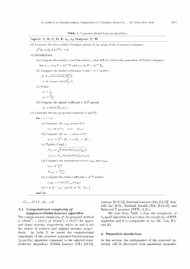
Table 1. Lyapunov-global-Lanczos algorithm.

Inputs: A, B, C, D, E, s1, s2; Outputs: V, W

(1) Generate the observability Gramian matrix Ro by using of the Lyapunov technique:

ATRo +RoA+ CTC = 0

(2) Initialization:

(a) Compute the matrix � and the vector �, that will be used in the generation of Krylov subspace:

Set � = �(s1E �A)�1E and � = (s2E �A)�1Ro1(b) Compute the initial coe�cients � and of T matrix:

�1 =p

trace(abs(�RTo1))

1 = �1trace(abs(RTo1�))

(c) De�ne:

v1 = ��1

w1 = Ro1 1

(d) Compute the initial coe�cient � of T matrix:

�1 = trace(RTo1�v1)

(3) Generate the two projection matrices V and W :

for i = 1 : m

(a) Compute the vi+1 vector of V :

vi+1 = � � vi � �ivi � �vi�1

(b) Compute the wi+1 vector of W :

wi+1 = �T �Roi � �iRoi � Roi�1

(c) Update � and

�i+1 =q

trace(abs(vi+1wTi+1))

i+1 = �i+1trace(abs(wTi+1vi+1))

(d) Compute the normalized vectors vi+1 and wi+1:

vi+1 = vi+1 i+

Roi+1 = wi+1�i+1

(e) Compute the other coe�cient � of T matrix:

�i+1 = trace(RToi+1�vi+1)

(f) V = [V vi+1] and W = [W Ri+1]

end for

Cm = C � V; Dm = 0:

3.1. Computational complexity ofLyapunov-Global-Lanczos algorithm

The computational complexity of the proposed methodis O(nm2) + O(n2) or O(mn2) + O(n3) for sparseand dense systems, respectively, where m and n arethe orders of reduced and original systems, respec-tively. In Table 2, we report the computationalcomplexity of the proposed Lyapunov-Global-Lanczos(Lyap-GL) algorithm compared to the selected state-of-the-art algorithms (Global Lanczos (GL) [18,21],

Lanczos [9,15,22], Rational Lanczos (RL) [21,23], Arn-odli (Ar) [9,24], Rational Arnoldi (RA) [9,14,19], andBalanced Truncation (BTR) [9,25]).

We note from Table 2 that the complexity ofLyap-Gl algorithm is lower than the complexity of BTRalgorithm and it is comparable to Ar, GL, Lan, RA,and RL.

4. Numerical simulations

In this section, the performance of the proposed ap-proach will be illustrated with simulation examples.


Table 2. Computational complexity.

Methods Sparsecomplexity

Densecomplexity

SparseLyapunov resolution

complexity

DenseLyapunov resolution

complexityLya-GL O(nr2) O(rn2) O(n2) O(n3)

Ar O(nr2) O(rn2) { {GL O(rn2) O(rn2) { {

BTR O(n2) O(n3) O(n2) O(n3)Lan O(nr2) O(rn2) { {RL O(nr2) O(rn2) { {RA O(nr2) O(rn2) { {

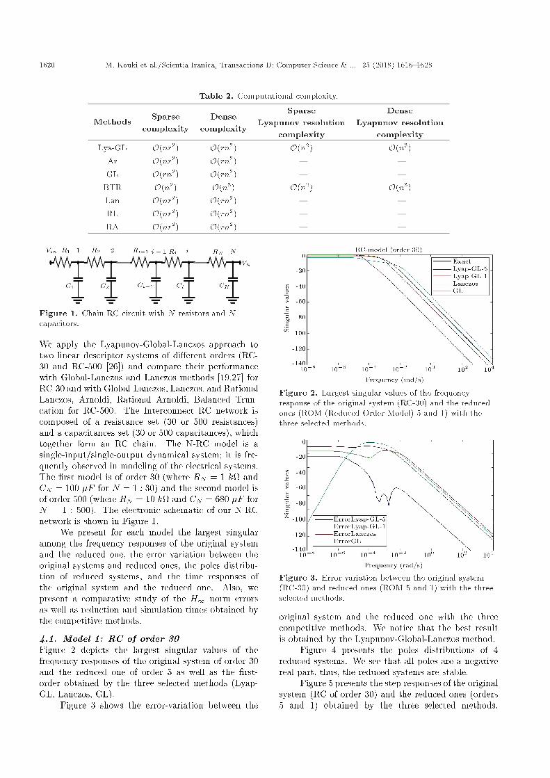
Figure 1. Chain RC circuit with N resistors and Ncapacitors.

We apply the Lyapunov-Global-Lanczos approach totwo linear descriptor systems of di�erent orders (RC-30 and RC-500 [26]) and compare their performancewith Global-Lanczos and Lanczos methods [19,27] forRC-30 and with Global-Lanczos, Lanczos, and RationalLanczos, Arnoldi, Rational Arnoldi, Balanced Trun-cation for RC-500. The Interconnect RC network iscomposed of a resistance set (30 or 500 resistances)and a capacitances set (30 or 500 capacitances), whichtogether form an RC chain. The N-RC model is asingle-input/single-output dynamical system; it is fre-quently observed in modeling of the electrical systems.The �rst model is of order 30 (where RN = 1 k andCN = 100 �F for N = 1 : 30) and the second model isof order 500 (where RN = 10 k and CN = 680 �F forN = 1 : 500). The electronic schematic of our N-RCnetwork is shown in Figure 1.

We present for each model the largest singularamong the frequency responses of the original systemand the reduced one, the error variation between theoriginal systems and reduced ones, the poles distribu-tion of reduced systems, and the time responses ofthe original system and the reduced one. Also, wepresent a comparative study of the H1 norm errorsas well as reduction and simulation times obtained bythe competitive methods.

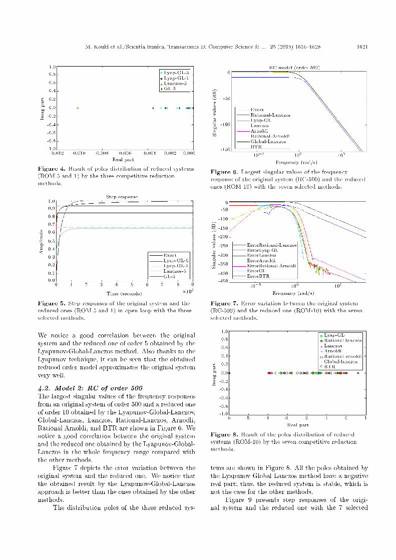
4.1. Model 1: RC of order 30Figure 2 depicts the largest singular values of thefrequency responses of the original system of order 30and the reduced one of order 5 as well as the �rst-order obtained by the three selected methods (Lyap-GL, Lanczos, GL).

Figure 3 shows the error-variation between the

Figure 2. Largest singular values of the frequencyresponse of the original system (RC-30) and the reducedones (ROM (Reduced Order Model) 5 and 1) with thethree selected methods.

Figure 3. Error-variation between the original system(RC-30) and reduced ones (ROM 5 and 1) with the threeselected methods.

original system and the reduced one with the threecompetitive methods. We notice that the best resultis obtained by the Lyapunov-Global-Lanczos method.

Figure 4 presents the poles distributions of 4reduced systems. We see that all poles are a negativereal part, thus, the reduced systems are stable.

Figure 5 presents the step responses of the originalsystem (RC of order 30) and the reduced ones (orders5 and 1) obtained by the three selected methods.


Figure 4. Result of poles distribution of reduced systems(ROM 5 and 1) by the three competitive reductionmethods.

Figure 5. Step responses of the original system and thereduced ones (ROM 5 and 1) in open loop with the threeselected methods.

We notice a good correlation between the originalsystem and the reduced one of order 5 obtained by theLyapunov-Global-Lanczos method. Also thanks to theLyapunov technique, it can be seen that the obtainedreduced order model approximates the original systemvery well.

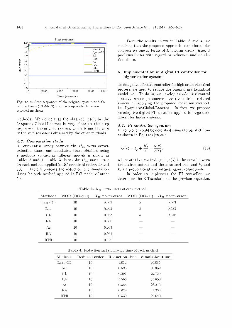
4.2. Model 2: RC of order 500The largest singular values of the frequency responsesfrom an original system of order 500 and a reduced oneof order 10 obtained by the Lyapunov-Global-Lanczos,Global-Lanczos, Lanczos, Rational-Lanczos, Arnodli,Rational Arnoldi, and BTR are shown in Figure 6. Wenotice a good correlation between the original systemand the reduced one obtained by the Lyapunov-Global-Lanczos in the whole frequency range compared withthe other methods.

Figure 7 depicts the error variation between theoriginal system and the reduced one. We notice thatthe obtained result by the Lyapunov-Global-Lanczosapproach is better than the ones obtained by the othermethods.

The distribution poles of the three reduced sys-

Figure 6. Largest singular values of the frequencyresponse of the original system (RC-500) and the reducedones (ROM-10) with the seven selected methods.

Figure 7. Error variation between the original system(RC-500) and the reduced one (ROM-10) with the sevenselected methods.

Figure 8. Result of the poles distribution of reducedsystems (ROM-10) by the seven competitive reductionmethods.

tems are shown in Figure 8. All the poles obtained bythe Lyapunov-Global-Lanczos method have a negativereal part; thus, the reduced system is stable, which isnot the case for the other methods.

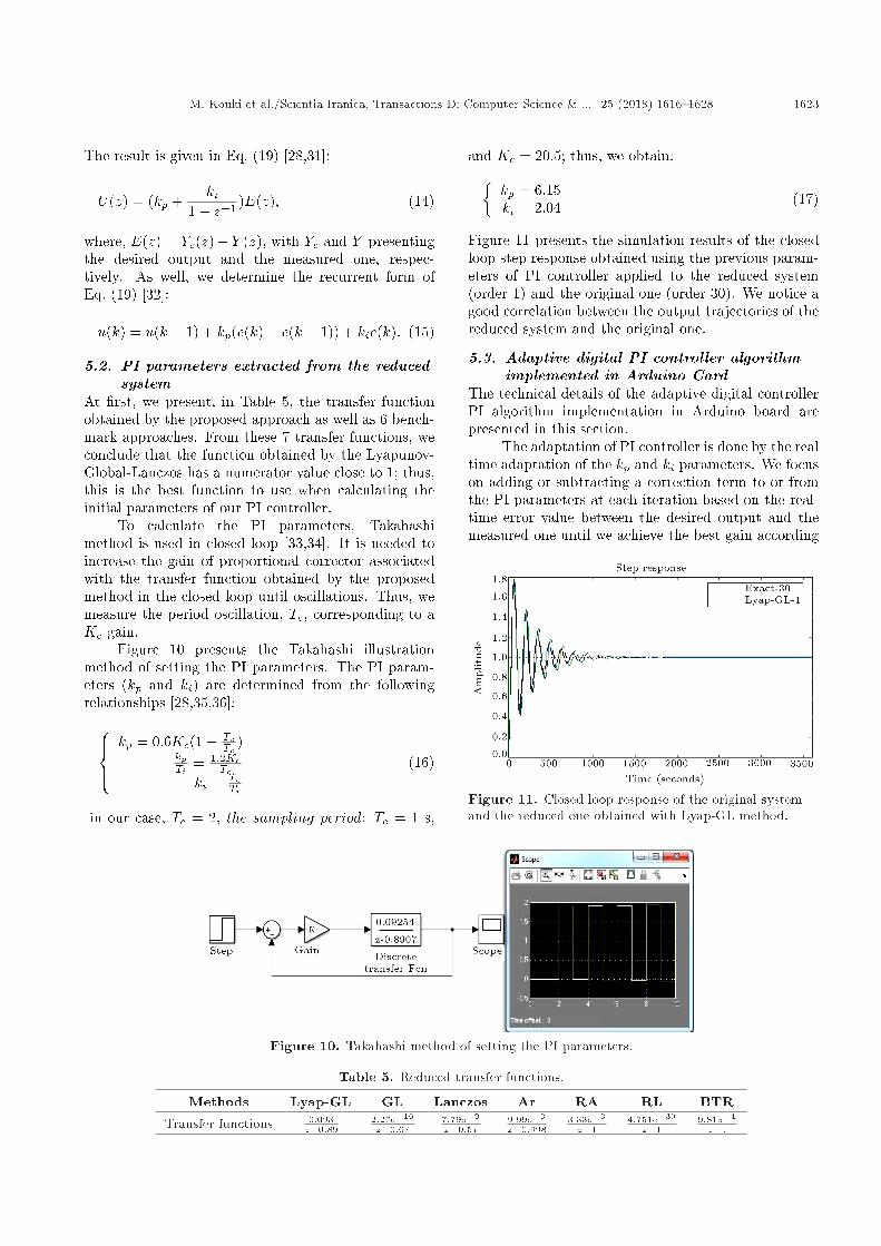
Figure 9 presents step responses of the origi-nal system and the reduced one with the 7 selected


Figure 9. Step responses of the original system and thereduced ones (ROM-10) in open loop with the sevenselected methods.

methods. We notice that the obtained result by theLyapunov-Global-Lanczos is very close to the stepresponse of the original system, which is not the caseof the step responses obtained by the other methods.

4.3. Comparative studyA comparative study between the H1 norm errors,reduction times, and simulation times obtained using7 methods applied in di�erent models is shown inTables 3 and 4. Table 3 shows the H1 norm errorfor each method applied in RC models of orders 30 and500. Table 4 presents the reduction and simulationtimes for each method applied in RC model of order500.

From the results shown in Tables 3 and 4, weconclude that the proposed approach outperforms thecompetitive one in terms of H1 norm errors. Also, itperforms better with regard to reduction and simula-tion times.

5. Implementation of digital PI controller forhigher order systems

To design an e�ective controller for high order electricalprocess, we need to reduce the original mathematicalmodel [28]. To do so, we develop an adaptive controlstrategy whose parameters are taken from reducedsystem by applying the proposed reduction method,i.e. Lyapunov-Global-Lanczos. In fact, we proposean adaptive digital PI controller applied to large-scaledescriptor linear systems.

5.1. PI controller equationPI controller could be described using the parallel fromas shown in Eq. (13) [29,30]:

G(s) = kp +Ki

s=u(s)e(s)

; (13)

where u(s) is a control signal, e(s) is the error betweenthe desired output and the measured one, and kp andki are proportional and integral gains, respectively.

In order to implement the PI controller, wedetermine the Z-Transform of the previous equation.

Table 3. H1 norm errors of each method.

Methods MOR (RC-500) H1 norm error MOR (RC-30) H1 norm error

Lyap-GL 10 0.001 5 0.003

Lan 10 0.003 5 0.533

GL 10 0.033 5 0:946

RL 10 0.030 { {

Ar 10 0.003 { {

RA 10 0.051 { {

BTR 10 0.539 { {

Table 4. Reduction and simulation time of each method.

Methods Reduced order Reduction-time Simulation-time

Lyap-GL 10 1.012 20.035Lan 10 0.526 30.352GL 10 0.297 29.720RL 10 5.566 33.650Ar 10 0:565 26.213RA 10 0:629 31.233

BTR 10 0:539 29.640


The result is given in Eq. (19) [28,31]:

U(z) = (kp +ki

1� z�1 )E(z); (14)

where, E(z) = Yc(z)� Y (z), with Yc and Y presentingthe desired output and the measured one, respec-tively. As well, we determine the recurrent form ofEq. (19) [32]:

u(k) = u(k � 1) + kp(e(k)� e(k � 1)) + kie(k): (15)

5.2. PI parameters extracted from the reducedsystem

At �rst, we present, in Table 5, the transfer functionobtained by the proposed approach as well as 6 bench-mark approaches. From these 7 transfer functions, weconclude that the function obtained by the Lyapunov-Global-Lanczos has a numerator value close to 1; thus,this is the best function to use when calculating theinitial parameters of our PI controller.

To calculate the PI parameters, Takahashimethod is used in closed loop [33,34]. It is needed toincrease the gain of proportional corrector associatedwith the transfer function obtained by the proposedmethod in the closed loop until oscillations. Thus, wemeasure the period oscillation, Tc, corresponding to aKc gain.

Figure 10 presents the Takahashi illustrationmethod of setting the PI parameters. The PI param-eters (kp and ki) are determined from the followingrelationships [28,35,36]:8><>: kp = 0:6Kc(1� Te

Tc )kpTi = 1:2Kc

Tcki = Te

Ti

(16)

in our case, Tc = 2, the sampling period: Te = 1 s,

and Kc = 20:5; thus, we obtain:�kp = 6:15ki = 2:04 (17)

Figure 11 presents the simulation results of the closedloop step response obtained using the previous param-eters of PI controller applied to the reduced system(order 1) and the original one (order 30). We notice agood correlation between the output trajectories of thereduced system and the original one.

5.3. Adaptive digital PI controller algorithmimplemented in Arduino Card

The technical details of the adaptive digital controllerPI algorithm implementation in Arduino board arepresented in this section.

The adaptation of PI controller is done by the realtime adaptation of the kp and ki parameters. We focuson adding or subtracting a correction term to or fromthe PI parameters at each iteration based on the real-time error value between the desired output and themeasured one until we achieve the best gain according

Figure 11. Closed loop response of the original systemand the reduced one obtained with Lyap-GL method.

Figure 10. Takahashi method of setting the PI parameters.

Table 5. Reduced transfer functions.

Methods Lyap-GL GL Lanczos Ar RA RL BTR

Transfer functions 0:093z�0:89

2:27e�16

z�0:677:79e�9

z�0:579:99e�3

z�0:9983:33e�3

z�14:751e�30

z�19:81e�4

z�1


to each input. It consists of an error value dependingon correction term between the desired output and themeasured one at each iteration. The adaptation termsare computed according to the following relationshipsEq. (18):

��p(k) = e(k � 1)=kp(k � 1)�i(k) = e(k � 1)=ki(k � 1) (18)

The new recurrent form of the PI controller is given by:

u(k) =u(k � 1) + (kp(k � 1)��p(k � 1))(e(k)

�e(k�1))+(ki(k�1)��i(k�1))e(k): (19)

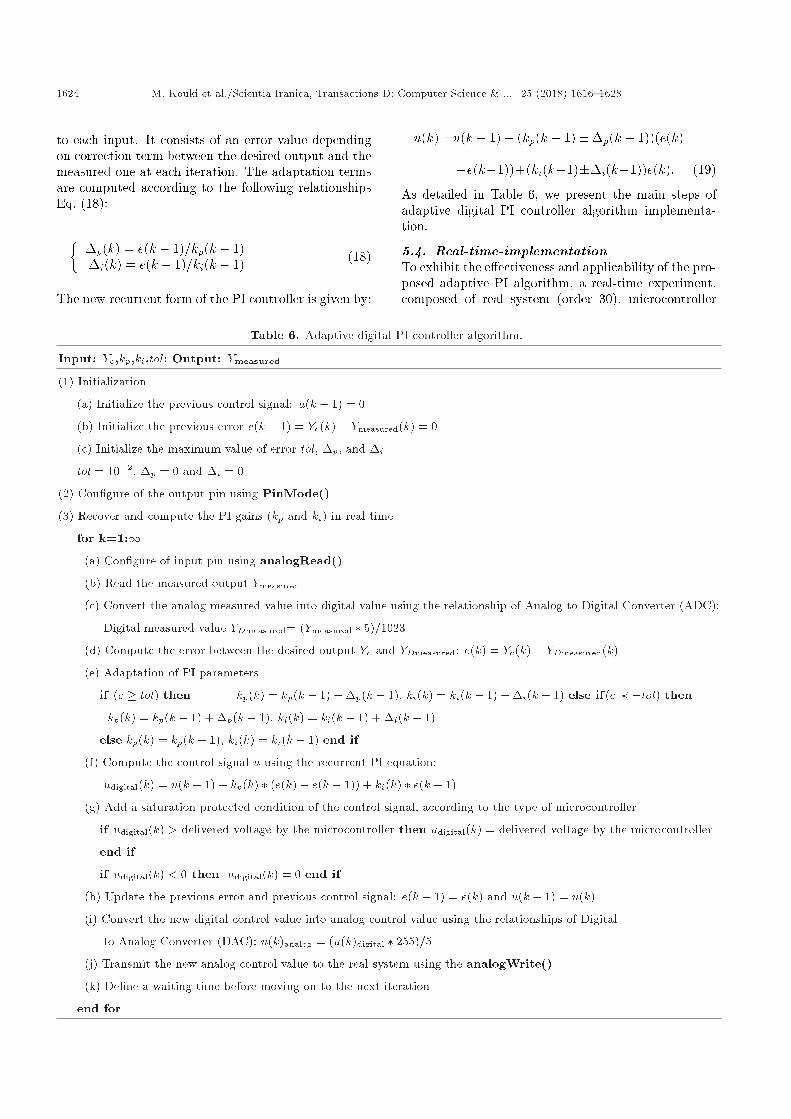
As detailed in Table 6, we present the main steps ofadaptive digital PI controller algorithm implementa-tion.

5.4. Real-time-implementationTo exhibit the e�ectiveness and applicability of the pro-posed adaptive PI algorithm, a real-time experiment,composed of real system (order 30), microcontroller

Table 6. Adaptive digital PI controller algorithm.

Input: Yc,kp,ki,tol; Output: Ymeasured

(1) Initialization

(a) Initialize the previous control signal: u(k � 1) = 0

(b) Initialize the previous error e(k � 1) = Yc(k)� Ymeasured(k) = 0

(c) Initialize the maximum value of error tol, �p, and �i

tol = 10�2, �p = 0 and �i = 0

(2) Con�gure of the output pin using PinMode()

(3) Recover and compute the PI gains (kp and ki) in real time

for k=1:1(a) Con�gure of input pin using analogRead()

(b) Read the measured output Ymeasured

(c) Convert the analog measured value into digital value using the relationship of Analog to Digital Converter (ADC):

Digital measured value YDmeasured= (Ymeasured � 5)=1023

(d) Compute the error between the desired output Yc and YDmeasured: e(k) = Yc(k)� YDmeasured(k)

(e) Adaptation of PI parameters

if (e � tol) then kp(k) = kp(k � 1)��p(k � 1), ki(k) = ki(k � 1)��i(k � 1) else if(e � �tol) then

kp(k) = kp(k � 1) + �p(k � 1), ki(k) = ki(k � 1) + �i(k � 1)

else kp(k) = kp(k � 1), ki(k) = ki(k � 1) end if

(f) Compute the control signal u using the recurrent PI equation:

udigital(k) = u(k � 1) + kp(k) � (e(k)� e(k � 1)) + ki(k) � e(k � 1)

(g) Add a saturation protected condition of the control signal, according to the type of microcontroller

if udigital(k) > delivered voltage by the microcontroller then udigital(k) = delivered voltage by the microcontroller

end if

if udigital(k) < 0 then udigital(k) = 0 end if

(h) Update the previous error and previous control signal: e(k � 1) = e(k) and u(k � 1) = u(k)

(i) Convert the new digital control value into analog control value using the relationships of Digital

to Analog Converter (DAC): u(k)analog = (u(k)digital � 255)=5

(j) Transmit the new analog control value to the real system using the analogWrite()

(k) De�ne a waiting time before moving on to the next iteration

end for


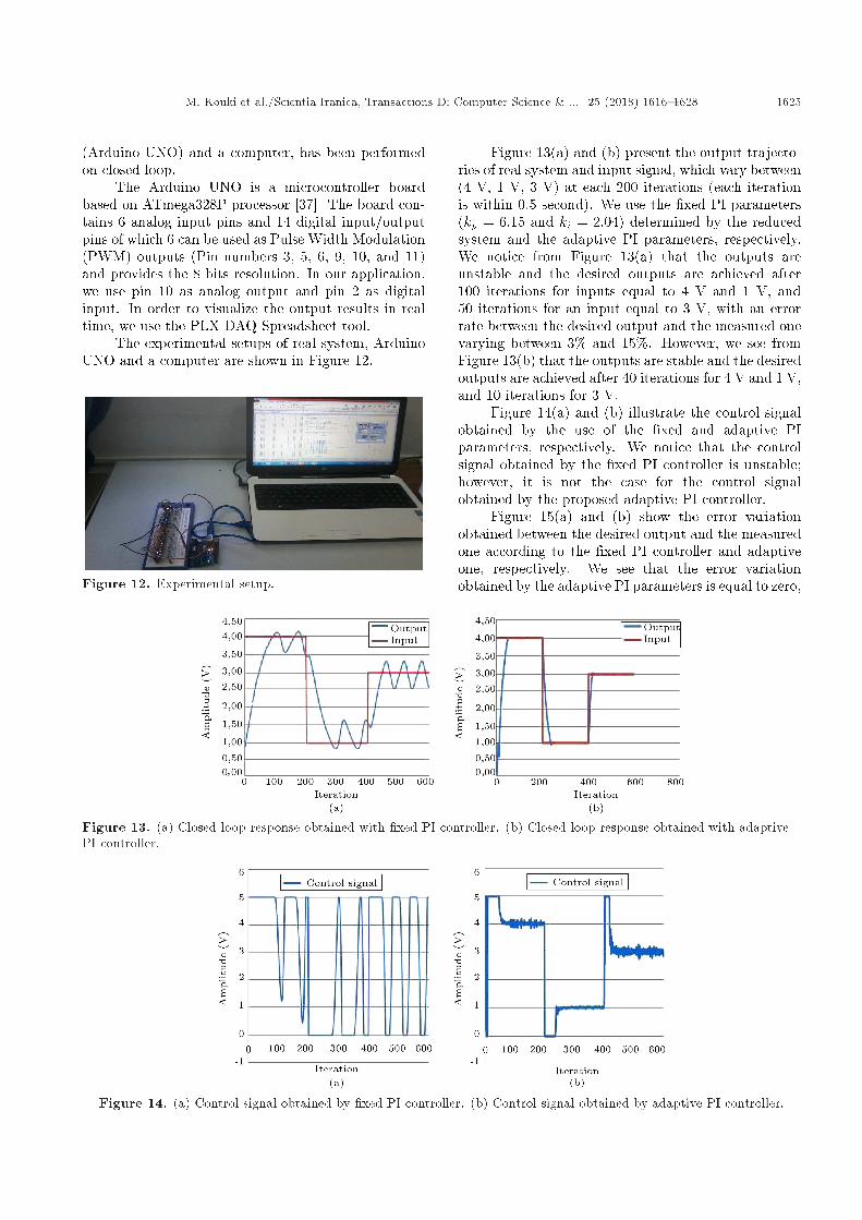
(Arduino UNO) and a computer, has been performedon closed loop.

The Arduino UNO is a microcontroller boardbased on ATmega328P processor [37]. The board con-tains 6 analog input pins and 14 digital input/outputpins of which 6 can be used as Pulse Width Modulation(PWM) outputs (Pin numbers 3, 5, 6, 9, 10, and 11)and provides the 8 bits resolution. In our application,we use pin 10 as analog output and pin 2 as digitalinput. In order to visualize the output results in realtime, we use the PLX-DAQ Spreadsheet tool.

The experimental setups of real system, ArduinoUNO and a computer are shown in Figure 12.

Figure 12. Experimental setup.

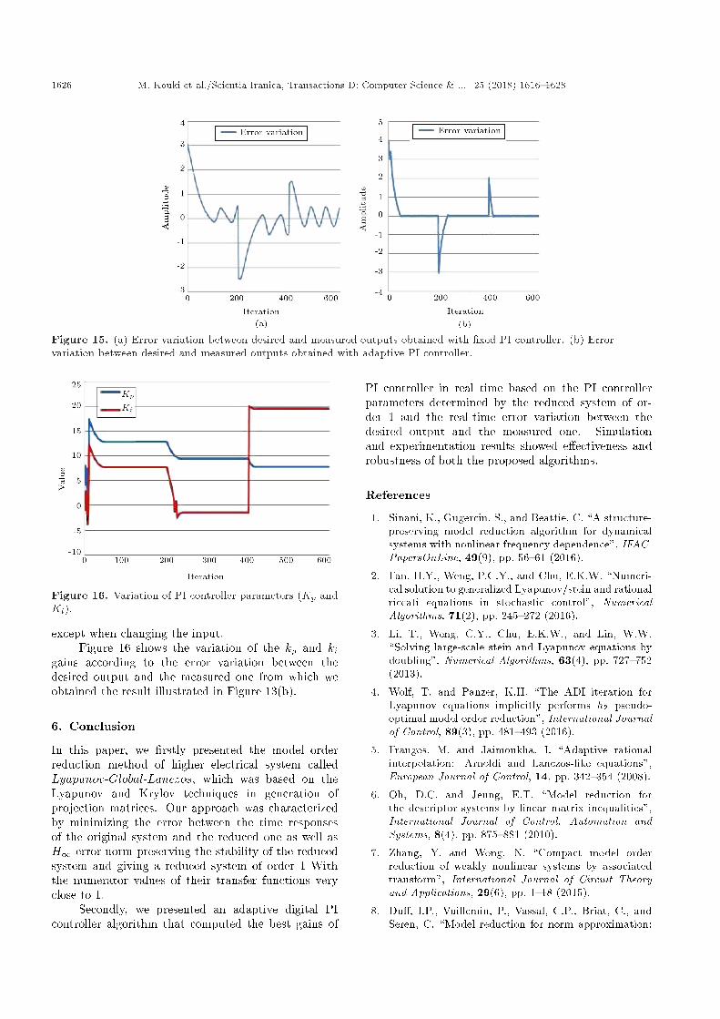
Figure 13(a) and (b) present the output trajecto-ries of real system and input signal, which vary between(4 V, 1 V, 3 V) at each 200 iterations (each iterationis within 0:5 second). We use the �xed PI parameters(kp = 6:15 and ki = 2:04) determined by the reducedsystem and the adaptive PI parameters, respectively.We notice from Figure 13(a) that the outputs areunstable and the desired outputs are achieved after100 iterations for inputs equal to 4 V and 1 V, and50 iterations for an input equal to 3 V, with an errorrate between the desired output and the measured onevarying between 3% and 15%. However, we see fromFigure 13(b) that the outputs are stable and the desiredoutputs are achieved after 40 iterations for 4 V and 1 V,and 10 iterations for 3 V.

Figure 14(a) and (b) illustrate the control signalobtained by the use of the �xed and adaptive PIparameters, respectively. We notice that the controlsignal obtained by the �xed PI controller is unstable;however, it is not the case for the control signalobtained by the proposed adaptive PI controller.

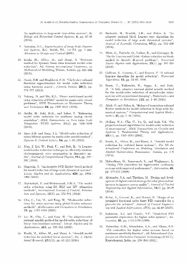
Figure 15(a) and (b) show the error variationobtained between the desired output and the measuredone according to the �xed PI controller and adaptiveone, respectively. We see that the error variationobtained by the adaptive PI parameters is equal to zero,

Figure 13. (a) Closed loop response obtained with �xed PI controller. (b) Closed loop response obtained with adaptivePI controller.

Figure 14. (a) Control signal obtained by �xed PI controller. (b) Control signal obtained by adaptive PI controller.


Figure 15. (a) Error variation between desired and measured outputs obtained with �xed PI controller. (b) Errorvariation between desired and measured outputs obtained with adaptive PI controller.

Figure 16. Variation of PI controller parameters (Kp andKi).

except when changing the input.Figure 16 shows the variation of the kp and ki

gains according to the error variation between thedesired output and the measured one from which weobtained the result illustrated in Figure 13(b).

6. Conclusion

In this paper, we �rstly presented the model orderreduction method of higher electrical system calledLyapunov-Global-Lanczos, which was based on theLyapunov and Krylov techniques in generation ofprojection matrices. Our approach was characterizedby minimizing the error between the time responsesof the original system and the reduced one as well asH1 error norm preserving the stability of the reducedsystem and giving a reduced system of order 1 Withthe numerator values of their transfer functions veryclose to 1.

Secondly, we presented an adaptive digital PIcontroller algorithm that computed the best gains of

PI controller in real time based on the PI controllerparameters determined by the reduced system of or-der 1 and the real-time error variation between thedesired output and the measured one. Simulationand experimentation results showed e�ectiveness androbustness of both the proposed algorithms.

References

1. Sinani, K., Gugercin, S., and Beattie, C. \A structure-preserving model reduction algorithm for dynamicalsystems with nonlinear frequency dependence", IFAC-PapersOnLine, 49(9), pp. 56{61 (2016).

2. Fan, H.Y., Weng, P.C.Y., and Chu, E.K.W. \Numeri-cal solution to generalized Lyapunov/stein and rationalriccati equations in stochastic control", NumericalAlgorithms, 71(2), pp. 245{272 (2016).

3. Li, T., Weng, C.Y., Chu, E.K.W., and Lin, W.W.\Solving large-scale stein and Lyapunov equations bydoubling", Numerical Algorithms, 63(4), pp. 727{752(2013).

4. Wolf, T. and Panzer, K.H. \The ADI iteration forLyapunov equations implicitly performs h2 pseudo-optimal model order reduction", International Journalof Control, 89(3), pp. 481{493 (2016).

5. Frangos, M. and Jaimoukha, I. \Adaptive rationalinterpolation: Arnoldi and Lanczos-like equations",European Journal of Control, 14, pp. 342{354 (2008).

6. Oh, D.C. and Jeung, E.T. \Model reduction forthe descriptor systems by linear matrix inequalities",International Journal of Control, Automation andSystems, 8(4), pp. 875{881 (2010).

7. Zhang, Y. and Wong, N. \Compact model orderreduction of weakly nonlinear systems by associatedtransform", International Journal of Circuit Theoryand Applications, 29(6), pp. 1{18 (2015).

8. Du�, I.P., Vuillemin, P., Vassal, C.P., Briat, C., andSeren, C. \Model reduction for norm approximation:


An application to large-scale time-delay systems", InDelays and Networked Control Systems, 6, pp. 37{55(2016).

9. Antoulas, A.C., Approximation of Large-Scale Dynam-ical Systems, R.C. Smith, Ed., 1st Ed. pp. 1{508,Advances in Design and Control (2005).

10. Kouki, M., Abbes, M., and Mami, A. \Svd-aoramethod for dynamic linear time invariant model orderreduction", 8th Vienna International Conference onMathematical Modelling, Vienna, Austria, pp. 695{696(2015).

11. Nasiri, S.H. and Maghfoori, F.M. \Chebyshev rationalfunctions approximation for model order reductionusing harmony search", Scientia Iranica, 20(3), pp.771{777 (2013).

12. Yuhang, D. and Wu, K.L. \Direct mesh-based modelorder reduction of PEEC model for quasi-static circuitproblems", IEEE Transactions on Microwave Theoryand Techniques, 64, pp. 2409{2422 (2016).

13. Aridhi, H., Zaki, H.M., and Tahar, S. \Enhancingmodel order reduction for nonlinear analog circuitsimulation", IEEE Transactions on Very Large ScaleIntegration (VLSI) Systems, 24(3), pp. 1036{1049(2016).

14. Xiao, Z.H. and Jiang, Y.L. \Model order reduction ofmimo bilinear systems by multi-order arnoldi method",Systems & Control Letters, 94, pp. 1{10 (2016).

15. J�orn, Z. Lei, W., Paul, U., and Rob, R. \A Lanczosmodel-order reduction technique to e�ciently simulateelectromagnetic wave propagation in dispersive me-dia", Journal of Computational Physics, 315, pp. 348{362 (2016).

16. Gugercin, S. \An iterative SVD-Krylov based methodfor model reduction of large-scale dynamical systems",Linear Algebra and Its Applications, 428, pp. 1964{1986 (2008).

17. Malekshahi, E. and Mohammadi, S.M.A. \The modelorder reduction using LS, RLS and MV estimationmethods", International Journal of Control, Automa-tion and Systems, 12(3), pp. 572{581 (2014).

18. Chu, C., Lai, M., and Feng, W. \Mode-order reduc-tions for mimo systems using global Krylov subspacemethods", Mathematics and Computers in Simulation,79, pp. 1153{1164 (2008).

19. Lee, H., Chu, C., and Feng, W. \An adaptive-orderrational arnoldi method for model-order reductions oflinear time-invariant systems", Linear Algebra and ItsApplications, 415, pp. 235{261 (2006).

20. Kouki, M., Abbes, M., and Mami, A. \Arnoldi modelreduction for switched linear systems", Int. J. Opera-tional Research, 27(1/2), pp. 85-112 (2016).

21. Barkouki, H., Bentbib, A.H., and Jbilou, K. \Anadaptive rational block Lanczos-type algorithm formodel reduction of large scale dynamical systems",Journal of Scienti�c Computing, 67(1), pp. 221{236(2016).

22. Silvia, G., Enyinda, O., Lothar, R., and Giuseppe, R.\On the Lanczos and Golub{Kahan reduction methodsapplied to discrete ill-posed problems", NumericalLinear Algebra with Applications, 23(1), pp. 187{204(2016).

23. Gallivan, K., Grimme, E., and Dooren, P. \A rationalLanczos algorithm for model reduction", NumericalAlgorithms, 12, pp. 33{63, 1996.

24. Bonin, T., Fa�bender, H., Soppa, A., and Zaeh,M. \A fully adaptive rational global arnoldi methodfor the model-order reduction of second-order mimosystems with proportional damping", Mathematics andComputers in Simulation, 122, pp. 1{19 (2016).

25. Abidi, O. and Jbilou, K. \Balanced truncation-rationalKrylov methods for model reduction in large scale dy-namical systems," Computational and Applied Mathe-matics, 35, pp. 1{16 (2016).

26. Meiling, W.J., Chu, C., Yu, Q., and Kuh, S.E. \Onprojection-based algorithms for model-order reductionof interconnects", IEEE Transactions on Circuits andSystems I: Fundamental Theory and Applications,49(11), pp. 1563{1585 (2002).

27. Kouki, K., Abbes, M., and Mami, A. \Arnoldi modelreduction for switched linear systems", The 5th In-ternational Conference on Modeling, Simulation andApplied Optimization, Hammamet, Tunisia, pp. 1{6(2013).

28. Malwatkara, G., Sonawaneb, S., and Waghmarec, L.\Tuning PID controllers for higher-order oscillatorysystems with improved performance", Automatica, 48,pp. 347-353 (2009).

29. Alexander, S.A. and Thathan, M. \Design and devel-opment of digital control strategy for solar photovoltaicinverter to improve power quality", Journal of ControlEngineering and Applied Information, 16(4), pp. 20-29(2014).

30. Rebai, A., Guesmi, K., and Hemici, B. \Design of anoptimized fractional order fuzzy PID controller for apiezoelectric actuator", Journal of Control Engineer-ing and Applied Information, 17(3), pp. 41-49 (2015).

31. Isakssona, A.J. and Graebe, S.F. \Analytical PIDparameter expressions for higher order systems", Au-tomatica, 35, pp. 1121-1130 (1999).

32. Malwatkar, G.M., Khandekar, A.A., and Nikam, S.D.\Pid controllers for higher order systems based onmaximum sensitivity function", 3th International Con-ference on Electronics Computer Technology (ICECT),Kanyakumari, India, pp. 259{263 (2011).


33. Franklin, G.F., Powell, J.D., and Workman, M.L.,Digital Control of Dynamic Systems, Addison andWesley (1990).

34. Kovacic, Z. and Bogdan, S., Fuzzy Controller Design:Theory and Applications, 19, CRC press (2005).

35. Gharib, M. and Moavenian, M. \Synthesis of robustPID controller for controlling a single input singleoutput system using quantitative feedback theory tech-nique", Scientia Iranica. Transaction B, MechanicalEngineering, 21(6), pp. 1861{1869 (2014).

36. Hasankola, M.D., Ehsaniseresht, A., Moghaddam, M.,and Saba, A. \Analysis, modeling, manufacturingand control of an elastic actuator for rehabilitationrobots", Scientia Iranica. Transaction B, MechanicalEngineering, 22(5), pp. 1855{1865 (2015).

37. Massimo, B. and David, C. \Arduino" (2016). [Online].Available: https://www.arduino.cc

Biographies

Mohamed Kouki was born in 1986 in Tunisia. Hereceived his MSc degree from the University of TunisELmanar at the Faculty of Sciences of Tunis in 2011.He received his PhD degree in Electrical Engineering

from the Faculty of Sciences of Tunis in 2014. His mainresearch interests include order reduction methods andcontrol algorithms in microelectronics.

Mehdi Abbes was born in 1978 in France. Hereceived the BSc degree in Electronics and Instru-mentation, in 2001, from the High School of Sciencesand Techniques of Tunis. In 2004, he obtained theMSc degree in measurement and instrumentation atthe High Institute of Applied Sciences and Technologyof Tunis. He received his PhD degree in ElectricalEngineering from the National School of Engineeringof Tunis, in 2009. His main research interests includebond graph modeling of thermo uid systems, reductionorder methods for large scale systems, control algo-rithms in microelectronics.

Abdelkader Mami was born in Tunisia. He isa Professor in Faculty of Sciences of Tunis. Hereceived his Dissertation H.D.R (Enabling to Directof Research) from the University of Lille (France) in2003; he is a member of Advice Scienti�c in Facultyof Science of Tunis. He is a President of commutatedthesis of electronics in the Faculty of Sciences of Tunis.

Date post:	17-Jul-2018
Category:	Documents
Upload:	duongmien
View:	230 times
Download:	0 times

Lyapunov-global-Lanczos algorithm for model order...

Documents