Lyapunov-Net: A Deep Neural Network Architecture for LyapunovFunction Approximation

Nathan Gaby1 Fumin Zhang2 Xiaojing Ye1

Abstract— We develop a versatile deep neural network archi-tecture, called Lyapunov-Net, to approximate Lyapunov func-tions of dynamical systems in high dimensions. Lyapunov-Netguarantees positive definiteness, and thus it can be easily trainedto satisfy the negative orbital derivative condition, which onlyrenders a single term in the empirical risk function in practice.This significantly reduces the number of hyper-parameterscompared to existing methods. We also provide theoreticaljustifications on the approximation power of Lyapunov-Net andits complexity bounds. We demonstrate the efficiency of theproposed method on nonlinear dynamical systems involving upto 30 dimensional state spaces, and show that the proposedapproach significantly outperforms the state-of-the-art methods.

I. INTRODUCTIONLyapunov functions play central roles in dynamical sys-

tems and control theory. They have been used to character-ize asymptotic stability of equilibria of nonlinear systems,estimate regions of attraction, investigate system robustnessagainst perturbations, and more [3], [7], [22]. In addition,Control Lyapunov functions are used to derive stabilizingfeedback control laws. The properties that Lyapunov func-tions must satisfy can be viewed as constrained partial differ-ential inequations (PDIs). However, like partial differentialequations (PDEs), for problems with high dimensional statespaces, it remains very challenging to compute approximatedLyapunov functions using classical numerical methods, suchas finite-difference method (FDM) and finite element method(FEM). The main issue is with the sizes of variables tosolve grows exponentially fast in terms of the state spacedimension of the problem using these classical methods.Such issue is known as the curse of dimensionality.

Recent years have witnessed a tremendous success of deeplearning (DL) methods in solving high-dimensional PDEs[6], [8], [21], [27]. Backed by the provable approximationpower [9], [10], [14], [19], [26], a (deep) neural networkcan fit very complicated functions accurately if the networksize (e.g., width and depth) is sufficiently large. Successfultraining of the parameters (e.g., weights and biases) of thenetwork approximating the solution of a PDE also requirea properly designed loss function and an efficient (non-convex) optimization algorithm. However, unlike traditionalDL-based methods in many classification and regressionapplications, the methods developed in [6], [21], [27] can

*The work is supported in part by National Science Foundation undergrants DMS-1818886 and DMS-1925263.

1Department of Mathematics and Statistics, Georgia State University,Atlanta, GA 30303, USA ngaby1,xye@gsu.edu

2School of Electrical and Computer Engineering, Georgia Institute ofTechnology, Atlanta, GA 30332, USA fumin@gatech.edu

directly approximate the solutions of specific PDEs usingdeep networks under certain conditions and do not requireany given training data but only need function and partialderivative (up to certain order depending on the PDE’s orderand the method used) evaluations at randomly sampled pointsin the problem domain.

Recently, deep neural networks (DNNs) also emergedto approximate Lyapunov functions of nonlinear dynamicalsystems in high-dimensional spaces [3], [7], [22]. For controlLyapunov functions, DNNs can also be used to approximatethe control laws, eliminating the restrictions on control lawsto specific function type (e.g., affine functions) in classicalcontrol methods such as linear-quadratic regulator (LQR).

In this work, we propose a unified framework to approxi-mate Lyapunov functions and control laws using deep neuralnets. Our main contributions lie in the following aspects:

• We propose a highly versatile network architecture, calledLyapunov-Net, to approximate Lyapunov functions. Specif-ically, this network architecture guarantees the desired pos-itive definiteness property and is very easy to implementin practice.

• We show that the training of Lyapunov-Nets is simpleand fast as they require much less manual hyper-parametertuning compared to existing methods, potentially allowingfor fast adoption of our method in a variety of problemsin practice.

• By employing recent results on deep network approxima-tion theory, we provide network complexity estimates ofthe proposed Lyapunov-Nets for guaranteed approximationaccuracy in high dimension.

• We apply the proposed Lyapunov-Net to solve severalbenchmark problems numerically. We show that ourmethod can effectively approximate Lyapunov functions(and associated control laws) in these problems with statedimension up to 30.

With the accuracy and efficiency of our method demonstratedin this work, we anticipate that our method can be appliedto a much broader range of dynamical system and controlproblems in high dimensions.

The remainder of the paper is organized as follows. In Sec-tion II, we review several notable results in the approximationpower of deep neural networks and the recent developmentsin approximating Lyapunov functions and control laws usingdeep learning methods. In Section III, we present our pro-posed network architecture and training strategies in details.In Section IV, we conduct numerical experiments using theproposed method on several nonlinear dynamical systems,

arX

iv:2

109.

1335

9v1

[cs

.LG

] 2

7 Se

p 20

21

demonstrating promising results on these tests. Section Vconcludes this paper.

II. RELATED WORK

In this section, we first provide an overview of the univer-sal approximation theory of (deep) neural networks, whichserves as the theoretical foundation for approximating contin-uous functions in arbitrary dimensions. Then we discuss therecent progresses in approximating Lyapunov functions andcontrol laws using DNNs and their relations to the presentwork.

a) Universal approximation theory of neural networks:The approximation powers of neural networks have beenstudied in the early 1990s. The asymptotic analysis justifiesthat shallow networks with one hidden layer and any non-polynomial activation function is dense in C1(Ω) for anycompact set Ω⊂Rd . However, the number of neurons neededto obtain a prescribed approximation accuracy of ε > 0may grow exponentially fast in d. Specifically, for shal-low networks with sigmoid activation function, it is shownthat a universal approximator of C1([−1,1]d) needs O(ε−d)computing neurons [9], [10]. The results are extended to(deep) ReLU neural networks in [14], [26]. Although deepneural networks are shown to be more effective in functionapproximation than shallow ones, the exponential depen-dency on problem dimension d still renders the curse ofdimensionality. In specific situations where the variables onlylie on a d′-dimensional (d′ < d) subspace (or manifold),one can employ a transformation so that the dependencyon d reduces to the dimensionality of the subspace, thusimproving the bound [19]. Similarly, if the variable can befactorized into decoupled components where all componentshave dimensionality no greater than d′, one can obtainsimilar bound O(ε−d′) with properly chosen DNN structure.However, in practice it can be difficult to justify that suchlow-dimensional structure or decoupling holds, and thereis still exponential dependency on d′ which can be large.There are also works developed to investigate the powerof DNNs in approximating other classes of functions. Inthe class of analytic functions, authors in [5], [18] showedthe exponential convergence speed based on the size of theapproximating network. The study of approximation powerof DNN remains an active research field [1], [2], [16].

b) Approximating Lyapunov function using neural net-works: Approximating Lyapunov functions using neuralnetworks can be dated back to [15], [25]. In [15] theauthors attempted the idea assuming that a shallow neuralnetwork can exact represent the target Lyapunov function. In[25], stabilization problem in control using neural networkswith one or two hidden layers are considered. In [20], theauthors propose a special shallow network to approximateLyapunov functions, however, the determination of the net-work parameters involves a series of constraints and Hessiancomputations. In [11], the control Lyapunov functions (CLF)using quadratic Lyapunov function candidate is considered.A DNN approach to CLF is considered in [3]. Approximatingstabilizing controllers using neural networks is considered

in [13]. Time discretized dynamics and successive parame-ter updates are considered in [22], [23]. Specifically, [22]considers to jointly learn the Lyapunov function and itdecreasing region which is expected to match the Regionof Attraction (ROA).

Special network architectures to approximate Lyapunovfunctions are also considered in [22]. In [22], a Lyapunovneural network of form ‖φθ (·)‖2 is proposed to ensurepositive semi-definiteness, where φθ (·) is a DNN. To ensurepositive definiteness, the authors restrict φθ to be a feed-forward neural network, all weight matrices to have fullcolumn rank, all biases to be zero, and all activation functionsto have trivial null space (e.g., tanh or leaky ReLU butnot sigmoid, swish, softmax or ReLU). Compared to thearchitecture in [22], the network architecture in the presentwork does not have any of these restrictions. Moreover,the positive definite weight matrix constructions in [22]can make ‖φθ (x)‖2 grow excessively fast as ‖x‖ increases,whereas ours does not have this issue.

In [7], the author considers dynamical systems with small-gain property, which yields a compositional Lyapunov func-tion structure that have decoupled components. In this case,it is shown that the size of the DNN used to approximatesuch Lyapunov functions can be dependent exponentially onthe maximal dimension of these components rather than theoriginal state space dimension.

III. PROPOSED METHOD

In this section, we propose the Lyapunov-Net architectureto approximate Lyapunov functions, and discuss its keyproperties and associated training strategies. We first recallthe definition of Lyapunov function for a given generaldynamical system x′ = f (x) with Lipschitz continuous f onthe problem domain Ω.

Definition 1 (Lyapunov function). Let Ω⊂Rd be a boundedopen set and 0 ∈ Ω, and f : Ω→ Rd a Lipschitz function.Then V : Ω→ R is called a Lyapunov function if (i) V ispositive definite, i.e., V (x)≥ 0 for all x ∈Ω and V (x) = 0 ifand only if x = 0; and (ii) V has negative orbital-derivative,i.e., DV (x) · f (x)< 0 for all x 6= 0.

Our goal is to build a neural network architecture thatis particularly suitable to approximate Lyapunov functionsfor any given f . We also demonstrate that the training ofLyapunov-Net renders a minimization problem of a simplerisk function, and thus requires much less manual hyper-parameter tuning and achievesy high optimization efficiencyduring practical computations.

A. Lyapunov-Net and its properties

Our main goal is to build a versatile deep network archi-tecture to approximate Lyapunov functions in state spacesof high dimension d, such that it is easy to implement andtrain, and performs efficiently in practice.

To this end, we first construct an arbitrary network φθ (·) :Rd×Rm with parameter θ . This network has input dimensiond and output dimension m (m∈N can be chosen arbitrarily).

Then we build a scalar-valued network Vθ : Rd→R from φθ

as follows:

Vθ (x) := ‖φθ (x)−φθ (0)‖2 +δ log(1+‖x‖2), (1)

where δ > 0 is a small user-chosen parameter and ‖·‖ is thestandard 2-norm. Then it is easy to verify that Vθ (0) = 0 and

Vθ (x)≥ δ log(1+‖x‖2)> 0, ∀x 6= 0.

In other words, Vθ is a candidate Lyapunov function thatalready satisfies the positive definiteness condition at equi-librium 0. We call the neural network Vθ with architecturespecified in (1) a Lyapunov-Net.

We make several remarks regarding the Lyapunov-Netarchitecture (1) below.

First, we use the augment term log(1 + ‖x‖2) to lowerbound the function Vθ (x) in order to ensure positive defi-niteness. One can also use ‖x‖2 which is sufficiently smoothand small near 0. Nevertheless, log(1 + ‖x‖2) ≈ ‖x‖2 asx→ 0, which means that it behaves very similar to ‖x‖2 nearthe equilibrium 0. Meanwhile, log(1+ ‖x‖2) ≈ 2log‖x‖ as‖x‖→∞, which grows very slowly and can potentially avoidforcing Vθ to be too large as ‖x‖ increases. In practice, onecan use any other positive definite function r :Rd→R+ suchthat r(x) = 0 if and only if x = 0, keeping in mind that suchr imposes an artificial lower bound of Vθ .

Second, the term ‖φθ (x)−φθ (0)‖2 in (1) can be replacedwith ψ(φθ (x)−φθ (0)) for any function ψ : Rm→ R+ suchthat ψ(0) = 0. The goal of this term is to ensure positivesemi-definiteness. We chose ψ(·) = ‖ · ‖2 for its simplicity.

Third, the choice of δ > 0 is arbitrary as Lyapunovfunctions can be arbitrarily scaled by a positive constant.Furthermore, we can avoid the ambiguity by applying abounded activation function (e.g., tanh) to the last, outputlayer of φθ . This ensures that φθ (x) is uniformly boundedfor all x and thus Vθ is bounded above.

Fourth, if the equilibrium is at x∗ instead of 0, then wecan simply replace φθ (0) and ‖x‖2 in (1) with φθ (x∗) and‖x−x∗‖2, respectively. Without loss of generality, we assumethe equilibrium is at 0 hereafter in this paper.

The properties remarked above show that Vθ defined in (1)serves as a versatile network architecture for approximatingLyapunov functions. As we will show soon, this architec-ture significantly eases network training and yields accurateapproximation of Lyapunov functions in practice.

B. Approximation power of Lyapunov-Net

The approximation power of Lyapunov-Net depends onseveral key factors. We here employ the universal approx-imation theorem of DNNs [9], [14], [26] to provide anestimate of the size of Lyapunov-Net for approximatingLyapunov functions. Assuming the target Lyapunov functionis in Cs(Ω) for some compact Ω and smooth level s∈N, wehave the following estimate for the approximation power ofLyapunov-Net.

Proposition 1. Let Ω ⊂ Rd be a simply connected openregion containing 0. Then for any ε ∈ (0,1) and s∈N, there

exists a ReLU neural network Vθ of the form (1) and sizeO(ε−d/s) such that for any Lyapunov function V ∈ Cs(Ω)corresponding to an f with equilibrium at 0, there is

‖Vθ −V‖L∞(Ω) := maxx∈Ω

|Vθ (x)−V (x)| ≤ ε

for a properly chosen θ .

Proposition 1 is a direct application of the universalapproximation theorem [9], [14], [26] in the context of Lya-punov function approximations. In practice, a much smallernetwork is sufficient in many examples to achieve ε errorwhen compared to the size estimate given in Proposition1. This gives some intuition that in many cases the aboveupper bound is not a tight one. We note more recent workssuch as [4], [24] and the references contained there in,show some of the new developments on these size bounds.Moreover, we can easily obtain the smaller network sizeestimate when the Lyapunov has compositional structure orhas lower dimensional structure. In the present work, we onlyconsider the most general scenario and do not adopt thesespecial problem or function structures.

C. Training of Lyapunov-Net

The training of Lyapunov-Net Vθ in (1) refers to finding aspecific network parameter θ such that the negative-orbital-derivative condition DVθ (x) · f (x) < 0 is satisfied at everyx ∈ Ω \ 0 and DVθ (0) · f (0) = 0. This can be achieve byminimizing a risk function that penalize Vθ if the negative-orbital-derivative condition fails to hold at some x. We canchoose the following as such risk function:

`(θ) :=1|Ω|

∫Ω

(DVθ (x) · f (x))2+ dx, (2)

where (z)+ := max(z,0) for any z ∈R. If strict negativity ofDVθ (x) · f (x) at all non-equilibrium point is strongly desired,we can replace DVθ (x) · f (x) with DVθ (x) · f (x)− δ ′γ(x)for any positive definite function γ(x), such as ‖x‖2 orlog(1+ ‖x‖2), as above, and δ ′ > 0 is a user-chosen smallvalue. It is clear that the risk function `(θ) reaches theminimal function value 0 if and only if DVθ (x) · f (x)≤ 0 (orDVθ (x) · f (x)≤ δ ′γ(x)) for all x ∈Ω, which, in conjunctionwith Vθ already being positive definite, ensures that Vθ is aLyapunov function. For notation simplicity, we use the form(2) assuming γ(x)≡ 0 hereafter.

In practice, the integral in (2) does not have analytic form,and we have to resort to Monte-Carlo integration whichis suitable for high-dimensional problems. To this end, wenotice that `(θ) = EX∼U(Ω)[(DVθ (X) · f (X))2

+] where U(Ω)stands for the uniform distribution on Ω (we assume it isbounded) and hence has distribution 1/|Ω|. Therefore, weapproximate `(θ) in (2) using the empirical expectation

ˆ(θ) :=1N

N

∑i=1

(DVθ (xi) · f (xi))2+, (3)

where xi : i ∈ [N] are independent and identically dis-tributed (i.i.d.) samples from U(Ω). Then we train theLyapunov-Net Vθ by minimizing ˆ(θ) in (3) with respect to

θ . Due to the explicit form of (3), standard network trainingalgorithms, such as ADAM [12] can be employed.

While ˆ(θ) in (3) is an unbiased estimator of `(θ) in(2), the variance of ˆ(θ) is known to be σ2

θ/N, where σ2

θ

stands for the variance of the integrand (DVθ (X) · f (X))2+

for X ∼ U(Ω). Therefore, an effective variance reductiontechnique to reduce σ2

θ, known as importance sampling (IS),

is to replace the uniform distribution U(Ω) with some moreadaptive distribution with density ρθ (x) (approximately) pro-portional to (DVθ (x) · f (x))2

+. In this case, we have `(θ) =EX∼ρθ

[ρ−1θ

(X)(DVθ (X) · f (X))2+], and thus

ˆIS(θ) :=1N

N

∑i=1

ρθ (xi)−1(DVθ (xi) · f (xi))

2+, (4)

where xi : i ∈ [N] are i.i.d. samples from ρθ . In this case,(4) is also an unbiased estimator of `(θ) in (2). However,the variance of ρ

−1θ

(X)(DVθ (X) · f (X))2+ with respect to

X ∼ ρθ is significantly smaller than σ2θ

as ρθ becomes moreproportional to (DVθ (x) · f (x))2

+. Therefore, in practice, onecan generate xi : i ∈ [N] from an easy-to-sample distribu-tion ρθ (e.g., mixture of Gaussian) which is approximatelyproportional to (DVθ (x) · f (x))2

+ for any given θ . In thiswork, we use uniform distribution U(Ω) and leave improvedsampling strategy such as IS for future investigation.

Several existing work [3], [7] observed that the deep-learning-based Lyapunov function approximation may vio-late the condition DVθ (x) · f (x)< 0 in a small neighborhoodof the equilibrium. Therefore, aside from the samplingstrategy above, we can add more sample points near theequilibrium 0 to mitigate this issue. By sampling morepoints near 0, we are essentially adding more weights tothe points there to ensure DVθ (x) · f (x) < 0. Since neuralnetworks implemented with smooth activation functions andbounded weights are by nature smooth functions, ensuringDVθ (x) · f (x) < 0 at a set of points densely sampled near 0can often lead to the condition being satisfied in the entireneighborhood.

It is worth stressing that the main advantage of theLyapunov-Net architecture (1) is that the risk function (2) (orthe empirical risk function (3)) consists of a single term only.This is in contrast to existing works [3], [7] where the riskfunctions have multiple terms to penalize the violations ofthe negative-orbital-derivative condition, positive definitenesscondition, bound requirements, etc. Thus, network trainingin these works requires experienced users to tune the hyper-parameters to properly weigh these penalty terms. On theother hand, the training of Lyapunov-Net Vθ proposed inthis work requires much less work in parameter-tuning andis computationally more efficient in practice.

D. Application to control and others

In light of the power of Lyapunov functions, we canemploy the proposed Lyapunov-Net to many control prob-lems of nonlinear dynamical systems in high-dimension. Inthis subsection, we instantiate one of such applications ofLyapunov-Net to approximate control Lyapunov function.

Consider a nonlinear control problem x′= f (x,u) where u :Rd →Rn (n is the dimension of the control variable at eachx) is an unknown state-dependent control in order to steerthe state x from any initial to the equilibrium state 0. To thisend, we parameterize the control as a deep neural networkuη : Rd → Rn (a neural network with input dimension dand output dimension n) where η represents the networkparameters of uη . In practice, the control variable is oftenrestricted to a compact set in Rd due to physical constraints.This can be easily implemented in a neural network setting.For example, if the magnitude of the control is required tobe in [−β ,β ] componentwisely, then we can simply applyβ · tanh(·) to the last, output layer of uη .

Once the network structure uη is determined, we candefine the risk of the control-Lyapunov function (CLF):

`CLF(θ ,η) :=1|Ω|

∫Ω

(DVθ (x) · f (x,uη(x)))2+ dx. (5)

Minimizing (5) yields the optimal parameters θ and η . Inpractice, we again approximate `CLF(θ ,η) by its empiricalexpectation ˆCLF(θ ,η) at sampled points in Ω, as an ana-logue to `(θ) versus ˆ(θ) above. Then the minimizationcan be implemented by alternately updating θ and η using(stochastic) gradient descent on the empirical risk functionˆCLF. Similar as (2), we have a single term in the lossfunction in (5), which does not have hyper-parameters totune and the optimization can be done efficiently.

IV. NUMERICAL EXPERIMENTSA. Experiment setting

We demonstrate the effectiveness of the proposed methodthrough a number of numerical experiments in this section.In our experiments, the value of δ used in (1) and thedepth and size of φθ used in Vθ for the three test problemsare summarized in Table I. We minimize the empirical riskfunction ˆ using the Adam Optimizer with learning rate 0.005and β1 = 0.9, β2 = 0.999 and Xavier initializer. In all tests,we iterate until the associated risk of (3) is below a prescribedtolerance 10−4. We use a sample size N (values shown inTable I), i.e., the number of sampled points in Ω in (3),such that the associated risk reduces reasonably fast whilemaintaining good uniform results over the domain.

All the implementations and experiments are performedusing PyTorch in Python 3.9 in Windows 10 OS on a desktopcomputer with an AMD Ryzen 7 3800X 8-Core Processor at3.90 GHz, 16 GB of system memory, and an Nvidia GeForceRTX 2080 Super GPU with 8 GB of graphics memory. Thenumber of iterations and training time (in seconds) for thethree tests are also given in Table I.

TABLE INETWORK PARAMETER SETTING AND TRAINING TIME IN THE TESTS.

Test Problem Time Iter. N Depth/Width δ

Curve Tracking 0.5 s 2 100K 3/10 0.530d Synthetic DS 2.3 s 15 400K 5/50 0.01Inverted Pendulum 20.4 s 579 400K 3/20 0.1

B. Experimental results

To demonstrate the effectiveness of the proposed method,we apply Lyapunov-Net (1) to three test problems: a two-dimensional (2d) nonlinear system from the curve-trackingapplication [17], a 30d synthetic dynamical system (DS)from [7], and a 2d inverted-pendulum system from [3]. In thefirst two problems, we aim at finding the Lyapunov functionfor the given dynamical systems, whereas in the last problemwe find both the Lyapunov function and the control u asdiscussed in Section III-D.

a) 2d DS in curve tracking: We apply our method tofind the Lyapunov function for a 2-dimensional (2d) nonlin-ear dynamical system (DS) in a curve-tracking application[17]. The dynamical system of x = (ρ,ϕ) is given by

ρ =−sin(ϕ), (6a)ϕ = (ρ−ρ0)cos(ϕ)−µ sin(ϕ)+ e. (6b)

We use the following constants in our experiments: e = 0.15,ρ0 = 1, and µ = 6.42 from [17] as well as ReLU activation.Figure 1 shows the approximated Lyapunov function Vθ

(top solid) and DVθ · f (bottom wire). We note the examplewas converted to Cartesian coordinates and graphed aroundcritical point x∗ = (1,0). The result shows after only 2 itera-tions the positive definiteness and negative-orbital-derivativeconditions are met.

x0.20.4

0.60.81.01.2

1.41.61.8

y −0.4−0.20.00.20.4

−1.5

−1.0

−0.5

0.0

0.5 1.0 1.5−0.50

−0.25

0.00

0.25

0.50

−1.5

−1.0

−0.5

0.0

Fig. 1. Left: Plot of the learned Lyapunov-Net Vθ (top solid) and DVθ · f(bottom wire) for the 2d system of the curve-tracking example convertedinto (x,y)-coordinates. Right: DVθ · f on the domain Ω.

b) 30d Synthetic DS: We consider a 30-dimensionalsynthetic DS with f obtained by stacking three copies of the10d DS from [7]. However, we do not impose any structuralinformation of the problem into our training. We note thisvector field defined on [−1,1]30 has an equilibrium at 0.Figure 2 graphed the approximated Lyapunov function Vθ

(top solid) and DVθ · f (bottom wire) in the (x2,x8) and(x10,x13) planes, using ReLU activation. These plots showthat Lyapunov-Net can effectively approximate Lyapunovfunctions in such high-dimensional problem.

c) Inverted Pendulum: The inverted pendulum is anoften considered problem in control theory see [3], [22]. Forthis problem we have dynamics x = (θ , θ) governed by

ml2θ = mgl sinθ −β θ +u, (7)

where u = u(x) is the control. We use g = 9.82, l = 0.5,m = 0.15, and β = 0.1 for our experiments.

Further, we adjust our model slightly so that we learn a upolicy alongside Vθ . This is done by implementing a single

x2−1.00−0.75−0.50−0.25

0.000.250.500.751.00

x8 −1.00−0.75−0.50−0.250.000.250.500.751.00

−5−4−3−2−1012

x10−1.00−0.75−0.50−0.25

0.000.250.500.75

1.00

x13−1.00−0.75−0.50−0.250.000.250.500.751.00

−3

−2

−1

0

1

2

Fig. 2. Plot of the learned Lyapunov-Net Vθ (top solid) and DVθ · f(bottom wire) in the (x2,x8)-plane (left) and (x10,x13)-plane (right) for the30d synthetic DS.

layer neural network u which performs a transform tanh(Ax)for some learned matrix A. The training method is the samefor both networks. We note that this network implementationof u allows for scaling of tanh to ensure u∈ [−β ,β ] for someconstrained region determined beforehand. Further, for otherexamples we could easily scale the network architecture of uto approximate more complex controls if desired. In Figure3, we use tanh as activation in Vtheta for smoothness of theplot. We note the error bounds are similar with ReLU buttanh has slightly better performance in this case.

angle−3 −2 −1 0 1 2 3angular velocity −3−2−10123

DVf, V

−50−40−30−20−10

0

−2 0 2−3

−2

−1

0

1

2

3

−50

−40

−30

−20

−10

0

Fig. 3. Left: learned Lyapunov-Net Vθ (top solid) and DVθ · f (bottomwire) for the 2d inverted pendulum in phase and angular velocity space.Right: DVθ · f on the domain Ω.

C. Comparison with existing methods

To demonstrate the significant improvement of Lyapunov-Net over existing methods in approximation efficiency, wecompare the proposed Lyapunov-Net to two recent ap-proaches [3], [7] that also use deep neural networks toapproximate Lyapunov functions in continuous DS setting.Specifically, we use the 30d synthetic DS as the test problemin this comparison.

Both [3], [7] employ generic deep network structure ofVθ , and thus require additional terms in their risk functionsto enforce positive definiteness of the networks. Specifically,the following risk function is used from [7]:

ˆ1(θ) = 1N

N∑

i=1

((DVθ (xi) · f (xi)+‖xi‖2

)2+

(8)

+(20‖xi‖2−Vθ (xi)

)2++(Vθ (xi)−0.2‖xi‖2)2

+

),

which aims at an approximate Lyapunov function Vθ satis-fying 0.2‖x‖2 ≤Vθ (x)≤ 20‖x‖2 and DVθ (x) · f (x)≤−‖x‖2

for all x. In [3], the following risk function is used:

ˆ2(θ) =Vθ (0)2 + 1N

N∑

i=1[(DVθ (xi) · f (xi))++(−Vθ (xi))+],

(9)

which aims at an approximate Lyapunov function Vθ suchthat Vθ (0) = 0, Vθ (x)≤ 0 and DVθ (x) · f (x)≤ 0 for all x. Theactivation functions are set to softmax in (8) as suggested in[7] and tanh in (9) as suggested in [3] For Lyapunov-Netwe use (3) as it already satisfies the positive definitenesscondition. We again do not impose any structural informationof the problem into our training, and thus all test methodsrecognize the DS as a generic 30d system for sake of a faircomparison.

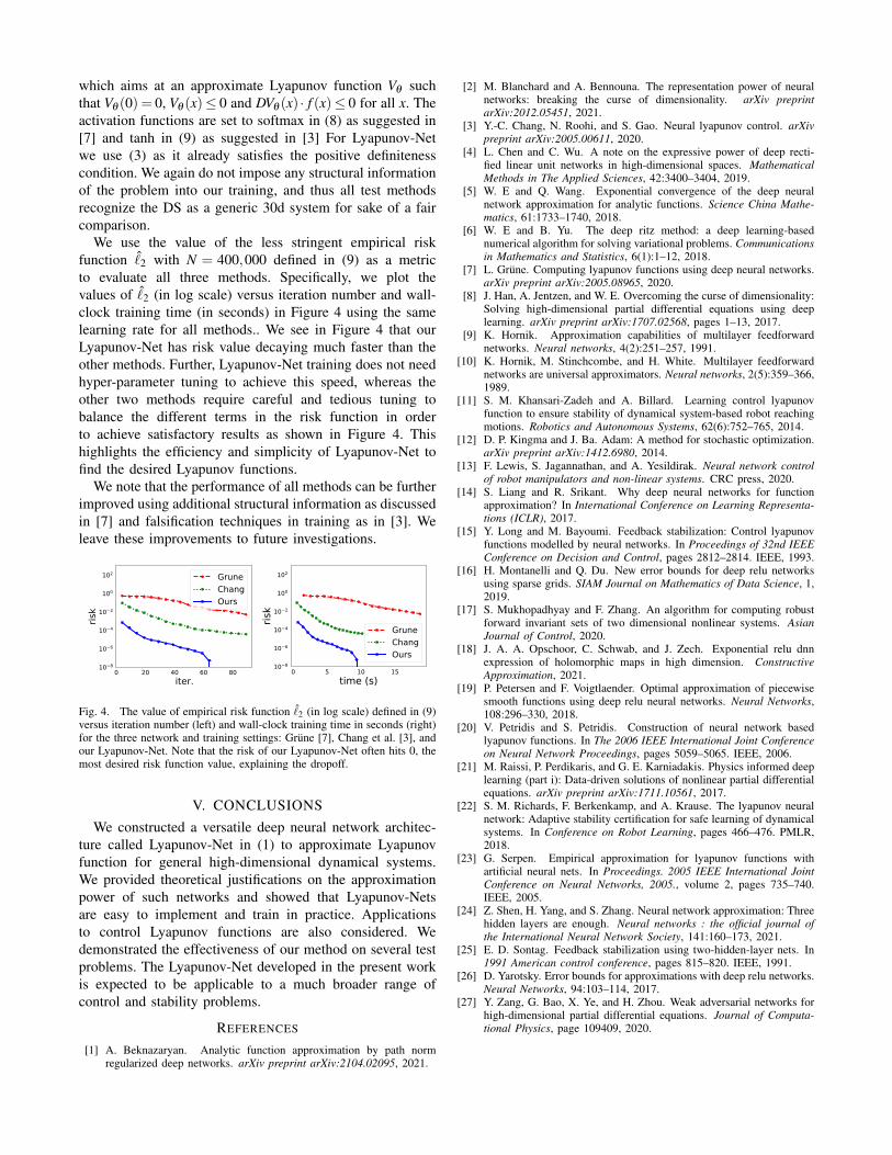
We use the value of the less stringent empirical riskfunction ˆ2 with N = 400,000 defined in (9) as a metricto evaluate all three methods. Specifically, we plot thevalues of ˆ2 (in log scale) versus iteration number and wall-clock training time (in seconds) in Figure 4 using the samelearning rate for all methods.. We see in Figure 4 that ourLyapunov-Net has risk value decaying much faster than theother methods. Further, Lyapunov-Net training does not needhyper-parameter tuning to achieve this speed, whereas theother two methods require careful and tedious tuning tobalance the different terms in the risk function in orderto achieve satisfactory results as shown in Figure 4. Thishighlights the efficiency and simplicity of Lyapunov-Net tofind the desired Lyapunov functions.

We note that the performance of all methods can be furtherimproved using additional structural information as discussedin [7] and falsification techniques in training as in [3]. Weleave these improvements to future investigations.

0 20 40 60 80iter.

10−8

10−6

10−4

10−2

100

102

risk

GruneChangOurs

0 5 10 15time (s)

10−8

10−6

10−4

10−2

100

102

risk

GruneChangOurs

Fig. 4. The value of empirical risk function ˆ2 (in log scale) defined in (9)versus iteration number (left) and wall-clock training time in seconds (right)for the three network and training settings: Grune [7], Chang et al. [3], andour Lyapunov-Net. Note that the risk of our Lyapunov-Net often hits 0, themost desired risk function value, explaining the dropoff.

V. CONCLUSIONSWe constructed a versatile deep neural network architec-

ture called Lyapunov-Net in (1) to approximate Lyapunovfunction for general high-dimensional dynamical systems.We provided theoretical justifications on the approximationpower of such networks and showed that Lyapunov-Netsare easy to implement and train in practice. Applicationsto control Lyapunov functions are also considered. Wedemonstrated the effectiveness of our method on several testproblems. The Lyapunov-Net developed in the present workis expected to be applicable to a much broader range ofcontrol and stability problems.

REFERENCES

[1] A. Beknazaryan. Analytic function approximation by path normregularized deep networks. arXiv preprint arXiv:2104.02095, 2021.

[2] M. Blanchard and A. Bennouna. The representation power of neuralnetworks: breaking the curse of dimensionality. arXiv preprintarXiv:2012.05451, 2021.

[3] Y.-C. Chang, N. Roohi, and S. Gao. Neural lyapunov control. arXivpreprint arXiv:2005.00611, 2020.

[4] L. Chen and C. Wu. A note on the expressive power of deep recti-fied linear unit networks in high-dimensional spaces. MathematicalMethods in The Applied Sciences, 42:3400–3404, 2019.

[5] W. E and Q. Wang. Exponential convergence of the deep neuralnetwork approximation for analytic functions. Science China Mathe-matics, 61:1733–1740, 2018.

[6] W. E and B. Yu. The deep ritz method: a deep learning-basednumerical algorithm for solving variational problems. Communicationsin Mathematics and Statistics, 6(1):1–12, 2018.

[7] L. Grune. Computing lyapunov functions using deep neural networks.arXiv preprint arXiv:2005.08965, 2020.

[8] J. Han, A. Jentzen, and W. E. Overcoming the curse of dimensionality:Solving high-dimensional partial differential equations using deeplearning. arXiv preprint arXiv:1707.02568, pages 1–13, 2017.

[9] K. Hornik. Approximation capabilities of multilayer feedforwardnetworks. Neural networks, 4(2):251–257, 1991.

[10] K. Hornik, M. Stinchcombe, and H. White. Multilayer feedforwardnetworks are universal approximators. Neural networks, 2(5):359–366,1989.

[11] S. M. Khansari-Zadeh and A. Billard. Learning control lyapunovfunction to ensure stability of dynamical system-based robot reachingmotions. Robotics and Autonomous Systems, 62(6):752–765, 2014.

[12] D. P. Kingma and J. Ba. Adam: A method for stochastic optimization.arXiv preprint arXiv:1412.6980, 2014.

[13] F. Lewis, S. Jagannathan, and A. Yesildirak. Neural network controlof robot manipulators and non-linear systems. CRC press, 2020.

[14] S. Liang and R. Srikant. Why deep neural networks for functionapproximation? In International Conference on Learning Representa-tions (ICLR), 2017.

[15] Y. Long and M. Bayoumi. Feedback stabilization: Control lyapunovfunctions modelled by neural networks. In Proceedings of 32nd IEEEConference on Decision and Control, pages 2812–2814. IEEE, 1993.

[16] H. Montanelli and Q. Du. New error bounds for deep relu networksusing sparse grids. SIAM Journal on Mathematics of Data Science, 1,2019.

[17] S. Mukhopadhyay and F. Zhang. An algorithm for computing robustforward invariant sets of two dimensional nonlinear systems. AsianJournal of Control, 2020.

[18] J. A. A. Opschoor, C. Schwab, and J. Zech. Exponential relu dnnexpression of holomorphic maps in high dimension. ConstructiveApproximation, 2021.

[19] P. Petersen and F. Voigtlaender. Optimal approximation of piecewisesmooth functions using deep relu neural networks. Neural Networks,108:296–330, 2018.

[20] V. Petridis and S. Petridis. Construction of neural network basedlyapunov functions. In The 2006 IEEE International Joint Conferenceon Neural Network Proceedings, pages 5059–5065. IEEE, 2006.

[21] M. Raissi, P. Perdikaris, and G. E. Karniadakis. Physics informed deeplearning (part i): Data-driven solutions of nonlinear partial differentialequations. arXiv preprint arXiv:1711.10561, 2017.

[22] S. M. Richards, F. Berkenkamp, and A. Krause. The lyapunov neuralnetwork: Adaptive stability certification for safe learning of dynamicalsystems. In Conference on Robot Learning, pages 466–476. PMLR,2018.

[23] G. Serpen. Empirical approximation for lyapunov functions withartificial neural nets. In Proceedings. 2005 IEEE International JointConference on Neural Networks, 2005., volume 2, pages 735–740.IEEE, 2005.

[24] Z. Shen, H. Yang, and S. Zhang. Neural network approximation: Threehidden layers are enough. Neural networks : the official journal ofthe International Neural Network Society, 141:160–173, 2021.

[25] E. D. Sontag. Feedback stabilization using two-hidden-layer nets. In1991 American control conference, pages 815–820. IEEE, 1991.

[26] D. Yarotsky. Error bounds for approximations with deep relu networks.Neural Networks, 94:103–114, 2017.

[27] Y. Zang, G. Bao, X. Ye, and H. Zhou. Weak adversarial networks forhigh-dimensional partial differential equations. Journal of Computa-tional Physics, page 109409, 2020.