Page 1
JSC 09384
CROP IDENTIFICATION TECHNOLOGY ASSESSMENT
FOR REMOTE SENSING (CITARS)
VOLUME I
TASK DESIGN PLAN
National Aeronautics and Space Administration
LYNDON B. JOHNSON SPACE CENTERHouston, TexasFebruary 1975
https://ntrs.nasa.gov/search.jsp?R=19760005366 2020-05-14T21:41:08+00:00Z
Page 2
T E C H N I C A L REPORT INDEX/ABSTRACT
1. TITLE AND SUBTITLE OF DOCUMENT
Crop Identification Technology AssesRemote Sensing (CITARS) , Volume I, 1Plan
Lockheed Electronics Company, Inc.
5. CONTRACTOR/ORIGINATOR DOCUMENT NO .
LEC-4326A
Unclassified
3. L I M i r A T f O N S ^_^
GOVERNMENT HAS UNLIMITED RIGHTS [ JYES [ XJ N0
11. DOCUMENT CONTRACT R E F E R E N C E S
WORK BREAKDOWN STRUCTURE NO.
Job Order 71-645CONTRACT E X H I B I T NO.
DAL NO. AND R E V I S I O N
DRL L I N E 1 TEM NO .
2 . JSC NO.
isment for JSC- 09384
NAS9-12200
6, PUBLICATION DATE (THIS ISSUE)
March 197.5
Earth Observations Division
IO. AUTHORISE
Dr. Forrest G. Hall, NASA TF7Robert M. Bizzell, NASA TF7
12. «<ROI«»£ CO»F I C U » » T I O N
SYSTEM
ERIPS, LARSYSSUBSYSTEM
Univac 1108/1110
13. ABSTRACT
This document sets out the design plan for a joint task to quantifythe crop identification performances resulting from the remote identifica-tion of corn, soybeans, and wheat. Automatic data processing techniquesdeveloped by the Earth Observations Division of the Lyndon B. JohnsonSpace Center of NASA, the Environmental Research Institute of Michigan,and the Laboratory for Applications of Remote Sensing of Purdue Universitywill be used in the quantification. The Agricultural Stabilization andConservation Service of the U.S. Department of Agriculture will assistthese three institutions in performing the task by furnishing ground-truthdata.
Steps for the conversion of multispectral data tapes to classifica-tion results will be specified. The crop identification performancesresulting from the use of several basic types of automatic data processingtechniques will be compared and examined for significant differences. Thetechniques will be evaluated also for changes in geographic location, timeof the year, management practices, and other physical factors.
The results of the Crop Identification Technology Assessment forRemote Sensing task will be applied extensively in the Large Area CropInventory Experiment.
M. S U B J E C T TEBIIS
Classmcationalgorithm Mnl m-ompn-ral rta + a Statistical ev^l liar- -jonCrop identificationpf»rfnrrnanoe> Quantification
RadiometricMultisoectral data preprocessina
Page 3
JSC 09384
CROP IDENTIFICATION TECHNOLOGY ASSESSMENT
FOR REMOTE SENSING (CITARS)
VOLUME I
TASK DESIGN PLAN
PREPARED BY
. Forrest G. Hall
APPROVED BY
_Dr. Andrew E. Potter, Chief
Research, Test, and Evaluation Branch
R. B. MacDonald, ChiefEarth Observations Division
NATIONAL AERONAUTICS AND SPACE ADMINISTRATIONLYNDON B. JOHNSON SPACE CENTER
HOUSTON, TEXAS
February 1975
Page 4
PREFACE
Because of the synoptic data acquisition capabilities
of satellites and high-altitude aircraft and the speed and
accuracy with which such data can be automatically processed,
there is a growing conviction that existing remote sensing
technology can be used to make crop inventories of much
larger areas than the relatively local areas for which this
technology was developed. The Crop Identification Technology
Assessment for Remote Sensing is being designed to evaluate
this capability. It will be an integral phase of the Large
Area Crop Inventory Experiment.
Participants in the task are the National Aeronautics
and Space Administration/Lyndon B. Johnson Space Center/
Earth Observations Division, the Environmental Research
Institute of Michigan, the Laboratory for Applications
of Remote Sensing of Purdue University, and the Goddard
Space Flight Center. The Agricultural Stabilization
Conservation Service of the U.S. Department of Agriculture
has agreed to support the task by collecting the ground-
truth data required to test the accuracy of the remote
sensing procedures. Personnel at the University of Houston,
the University of Texas at Dallas, and Rice University also
contributed to the preliminary planning.
The planned documentation for the activity of the Crop
Identification Technology Assessment for Remote Sensing is:
Volume I, Task Design Plan
Volume II, Ground Truth Data
Page 5
vi
Volume III, Data Acquisition
Volume IV, Image Analysis
Volume V, Data Preparation
Volume VI, Data Processing by the Laboratory for Appli-
cations of. Remote Sensing :
Volume VII, .Data Processing by the Environmental Research
Institute of Michigan ' ' ''
Volume VIII, Data Processing by the National Aeronautics
and Space Administration/Lyndon B. Johnson. Space Center/
Earth.Observations Division
Volume IX, Analysis of. Results
Volume X, Final Report
Page 6
VI1
ACKNOWLEDGMENTS
The author gratefully acknowledges the contributions
and invaluable assistance of the following persons in the
preparation of this Task Design Plan.
Dr. Marvin E. Bauer and Dr. Philip H. Swain, Laboratory
for Applications of Remote Sensing, Purdue University
Robert M. Bizzell, Earth Observations Division,
Lyndon B. Johnson Space Center, National Aeronautics
and Space Administration
Dr. Emil Jebe and Mr. William A. Malila, Environmental
Research Institute of Michigan
Page 7
GLOSSARY
ACORN4 — an algorithm used by the Environmental Research
Institute of Michigan for correcting data for scan-""' •'" •'•'"''•'." -
angle-dependent variations before classification
ADP — automatic data processing
ASCS — Agricultural Stabilization and Conservation Service
of the U.S. Department of Agriculture
BSI — Batch System Interface, a classification subsystem
of the Earth Resources Interactive Processing System
CCP — crop classification performance, level of crop
performance to be determined by analysis-of-variance
testing
CCT — computer-compatible tape containing digital satellite
data
CIP — crop identification performance, the quantitative
assessment of crop inventories in specified areas
using remote sensing, photointerpretation, and ADP
techniques
CITARS — Crop Identification Technology Assessment fors
Remote Sensing
>,' i " •. •
Clustering — a mathematical procedure for organizing multi-
spectral data into spectrally homogeneous groups
Page 8
CRT — cathode-ray tube
CY — calendar yearv ' • • • • ' - ; '
DAS — data analysis station, a computer system for reformat-
ting, analyzing, and reviewing digital, remotely sensed
data
DS&AD — Data Systems and Analysis Directorate of the
Lyndon B. Johnson Space Center, NASA
EOD — Earth Observations Division of the Lyndon B. Johnson
Space Center, NASA
EREP — Earth Resources Experiment Package, consisting of
remote sensors mounted on the Skylab spacecraft
ERIM — Environmental Research Institute of Michigan
ERIPS — Earth Resources Interactive Processing System, a
system at the Lyndon B. Johnson Space Center, NASA,
which provides real-time interaction of an investigator
with several digital, spectral analysis procedures
ERPO — Earth Resources Program Office at the Lyndon B. Johnson
Space Center, NASA
ERTS-1 — the first Earth Resources Technology Satellite,
which was launched in June 1972, orbits the Earth
14 times a day from an altitude of 915 kilometers,
and scans the same scene every 18 days
Page 9
XI
ERTS-B — the second Earth Resources Technology Satellite,
which will be launched in January 1975/
FOB — Flight Operations'Directorate of the Lyndon B. Johnson
Space Center, NASA
FY — fiscal year
GDSD — Ground Data Systems Division of the Lyndon B. Johnson
Space. Center, NASA . . - • - .
Gray map — a CRT digital image composed of a scale of
gray tones ,
Ground truth — data collected by ground observations of
the ASCS on selected sections for.the CITARS task
GSFC — Goddard Space Flight Center, NASA, located in
Greenbelt, Maryland .
ISOCLS — Iterative Self-Organizing Clustering System, a
computer program developed by the EOD which uses a
clustering algorithm to group homogeneous spectral
data
JSC — Lyndon B. Johnson Space Center of NASA
LACIE — Large Area Crop Inventory Experiment, which will
utilize the results of the CITARS task in future crop
inventories
Page 10
Xll
LACIP — Large Area Crop Inventory Project which was renamed
LACIE
LARS.— Laboratory for Applications of Remote .Sensing
of Purdue University
LARSYS — a system of classification programs developed at
the LARS
Local recognition — a condition for establishing CIP where
crop signatures for classifier training are obtained
from the geographic region in which the crops are
identified
LOE — level of effort, used to designate an undetermined
work force on a project when equivalent man-hours
cannot be accurately estimated
2MS— aircraft, modular, multiband 11-channel scanner
developed by The Bendix Corporation
M-7 — aircraft, modular, 12-channel scanner developed by
the ERIM
MIST — multispectral image tape, to which data are transferred
and stored at LARS
MSDS — Multispectral Data System at JSC, which includes an
aircraft 24-channel scanner and a ground DAS
Page 11
Xlll
MSP — multitemporal processing
MSS — multispectral scanner onboard the ERTS-1
NASA — National Aeronautics and Space Administration
Nonlocal recognition — a condition for establishing CIP
where crop signatures for classifier training are
obtained from a geographic region other than the one
in which the crops are identified
'NSA' — an ERIM computer descriptor used to specify the
input format for field boundary coordinates
PCM — pulse-code modulated
Pixel — a picture element which refers to one instantaneous
field of view as recorded by the ERTS-1 MSS and covers
the equivalent of 0.44 hectare (1.09 acres) (One ERTS-1
frame contains approximately 7.36 * 10 pixels.)
PSP — preprocessing and standard processing
PTD — Photographic Technology Division of JSC
Quarter section — one quarter of a section of land selected
for ASCS field visits
RTOP — Research and Technology Operational Plan
Page 12
XIV
S190A — multispectral photographic system on the Skylab
spacecraft
S190B — Earth terrain photographic system on the Skylab
spacecraft
S&AD — Science and Applications Directorate of JSC
Section — a 1.6- by 8-kilometer subdivision of the test
segment, selected for extraction of test data
SRS — Statistical Reporting Service of the U.S. Department
of Agriculture
SRT — Supporting Research and Technology, a team effort of
EOD, ERIM, and LARS
Test segment — an 8- by 32-kilometer (25,856-hectare or
64,600-acre) parcel of land selected for extracting
MSS data
UP — unresolved objects processing
USDA — U.S. Department of Agriculture
Page 13
XV
CONTENTS
Section Page
1.0 INTRODUCTION 1
1.1 TASK DESCRIPTION 1
1.2 BACKGROUND 2
1.2.1 Remote Sensing Data ProcessingProcedures 2
1.2.2 Large-Area InventoryProcedure 3
2.0 APPROACH 5
3.0 DETERMINATION OF TEST AREAS 9
3.1 TEST SITES 9
3.2 TEST SEGMENTS 10
3.3 SECTIONS 11
3.3.1 Quarter Sections n
3.3.2 Test Sections 11
3.4 FIELDS . 11
3.4.1 Training Fields 12
3.4.2 Pilot and Test Fields 12
4.0 DATA ACQUISITION 17
4.1 SPACECRAFT SCANNER DATA 18
4.1.1 ERTS-1 18
4.1.2 Skylab 19
4.2 AIRCRAFT SCANNER DATA 19
Page 14
XVI
Section Page
4.3 AIRCRAFT PHOTOGRAPHIC DATA 20
4.4 GROUND INVESTIGATIONS . . 22
4.4.1 Agricultural Data 22
4.4.2 Atmospheric Optical DepthData 23
5.0 DATA HANDLING 27
5.1 AIRCRAFT PHOTOGRAPHIC DATA 29
5.2 GROUND INVESTIGATION DATA 30
5.3 MSS DATA 30
5.3.1 Data Preparation 30
5.3.1.1 ERTS-1 data 31
5.3.1.2 EREP scanner data. . . 32
5.3.1.3 Aircraft scanner data(M2S, M-7, MSDS) ... 32
5.3.2 Data Processing 33
5.3.2.1 Standard ADPtechniques 34
5.3.2.2 ADP techniques withpreprocessing forsignature extension. . 36
5.3.2.3 ADP techniques formultitemporal andunresolved objects . . 38
5.4 PERFORMANCE COMPARISONS 39
5.5 EVALUATIONS OF CIP 42
5.5.1 Determination of SignificantDifferences in CIP's 42
Page 15
XV11
Section Page
5.5.2 Measures of Performance Using- - - - - - - - . - ADP Techniques. . . ." . . . . . 44
5.5.2.1 Factorial analysesfor performancecomparisons 45
5.5.2.2 Analysis ofvariance 46
6.0 TASK MANAGEMENT 49
6.1 TASK RESPONSIBILITY . . 49
6.1.1 EOD 49
6.1.2 ERIM 50
6.1.3 LARS 50
6.1.4 GSFC and USDA 50
6.2 SCHEDULING AND MILESTONES 50
6.2.1 Data Acquisition andDissemination 51
6.2.2 Establishment of ClassificationAccuracy 51
6.2.3 Performance Comparisons .... 51
6.2.4 Review and Documentation. ... 52
6.3 RESOURCE REQUIREMENTS 52
Page 16
XV111
Appendix ' Page
A , PROCEDURE FOR SECTION AND QUARTER" SECTION SELECTION WITHIN SEGMENTS ..... A-l
A.I SECTION AND QUARTER SECTIONSELECTION .............. A-l
A. 2 TEST SECTION SELECTION ........ A-3
B TRAINING, PILOT, AND TEST FIELDSELECTION PROCEDURES ........... B-l
B.I TRAINING FIELDS ...... . . . . . B-l
B.2 PILOT AND TEST FIELDS ........ B-l
C PROCEDURE FOR LOCATION OF FIELDBOUNDARIES
C.l GENERATE GRAY-SCALE MAPS ....... C-2
C.2 OUTLINE HIGHWAYS AND LANDMARKS. . . . C-2
C.3 LOCATE GROUND-TRUTH SECTIONS ..... C-2
C.4 LOCATE FIELD BOUNDARIES ....... C-3
C.5 DEFINE FIELD CENTERS ......... C-5
C.6 OBTAIN SECTION AND FIELD CARDS. . . . C-5
C.7 DISPLAY- AND CHECK BOUNDARIES ..... C-6
C.8 EDIT FOR SUBSEQUENT MISSIONS ..... C-6
C.9 PREPARE DECKS ............ C-7
D TEST SEGMENT SECTION LOCATIONSFOR TEST AND PILOT FIELDS ......... D-l
E PHOTOINTERPRETIVE PROCEDURES ....... E-l
E.I IMAGE INTERPRETATION PLAN ...... E-l
E.2 REPORTS ............... E-4
Page 17
XIX
Appendix Page
F . PROCEDURE FOR TESTING ACCURACY OFPHOTOINTERPRETATION . F-l
G DATA SCREENING AMD EVALUATIONPROCEDURES . G-l
G.I DATA QUALITY EVALUATIONS ATTHE EOD G-l
G.I.I Photographic Data. G-l
G.I. 2 Electronic Data G-2
G.I. 3 Reporting G-2
G.2 DATA QUALITY EVALUATIONS AT LARS. . . G-3
G.2.1 ERTS Data G-3
G.2.2 M-7 Scanner Data G-4
G.2.3 Reporting G-5
G.3 DATA QUALITY EVALUATIONS AT ERIM. . . G-5
G.3.1 ERTS Data G-5
G.3.2 Aircraft MSS Data G-8
H DATA PREPARATION PROCEDURES H-l
H.I REFORMATTING OF M2S DATA H-l
H.2 REFORMATTING OF AIRCRAFT MSS DATA . . H-l
H.3 PREPARATION OF ERTS DATA H-2
H.4 GEOMETRIC CORRECTION OFERTS DATA H-3
H.4.1 Scale Correction H-3
H.4.2 Earth Rotation SkewCorrection H-5
Page 18
XX
Appendix Page
H.4.3 Frame Rotation H-6
H.4.4 Rescaling . . . . H-7
H.5 TEMPORAL OVERLAY. . . . " . . - H-12
H.6 EFFECTS OF GEOMETRIC TRANSFORMATIONSON CIP H-16
H.7 . EFFECTS OF PROCESSING ON ANALYSISRESULTS H-17
I PROCEDURES FOR EOD ADP 1-1
1.1 ERTS-EOD-SP1 1-1
1.1.1 Local RecognitionProcessing 1-1
1.1.2 Nonlocal RecognitionProcessing 1-10
1.2 M2S-EOD-SP1 1-11
1.2.1 Local recognitionProcessing 1-12
1.2.2 Nonlocal recognitionProcessing 1-19
1.3 M2S-EOD-SP2 1-19
1.4 M2S-EOD-SP3 1-20
1.5 M2S-EOD-PSP1 1-21
1.6 ERTS-EOD-MSP1 1-21
1.7 M-7-EOD-SP1 1-23
1.8 M-7-EOD-SP2 1-23
Page 19
XXI
Appendix Page
1.9 CONTINGENCY PROCEDURES 1-22
1.9.1 Clustering/Statistics 1-23
1.9.2 Feature Selection 1-25
1.9.3 Classification 1-27
J LARS DATA ANALYSIS PROCEDURES J-l
J.I INTRODUCTION J-l
J.2 DATA ANALYSIS PROCEDURESSPECIFICATION J-l
J.2.1 General Procedures andRationale J-l
J.3 STEP-BY-STEP INSTRUCTIONS FORTHE DATA ANALYST J-l
J.3.1 ERTS-LARS-SP1 J-8
J.3.2 ERTS-LARS-SP2 J-14
J.3.3 Aircraft-LARS-SPl/SP2. .... J-15
K ERIM DATA PROCESSING AND ANALYSISPROCEDURES K-l
K.I ERTS MSS DATA K-2
K.I.I Reformatting of the data . . . K-2
K.I.2 Verification of DataQuality K-2
K.I.3 Conversion and Checking ofField Coordinates K-6
K.I.4 Definition of Major ClassSignatures K-8
Page 20
XX11
Appendix Page
K.I.5 Class "Other" Signatures . . . K-15
K.I.6 Classification WithoutPreprocessing (ERTS-ERIM-SP1) K-17
K.I.7 Classification withPreprocessing (ERTS-ERIM-PSP1) K-19
K.I.8 Postrecognition Analysis . . . K-22
K.I.9 Classification With theQuadratic Decision Rule. . . . K-23
K.I.10 Procedures for EstimatingProportions With a MixturesAlgorithm (ERTS-ERIM-SP3/SP4) K-24
K.2 AIRCRAFT MSS DATA K-34
K.2.1 Reformatting of the Data . . . K-34
K.2.2 Conversion of FieldCoordinates K-34
K.2.3 Verification of DataQuality K-34
K.2.4 Verification of FieldDelineations K-35
K.2.5 Preprocessing of Data forScan-Angle Variations(Aircraft-ERIM-PSP2) K-36
K.2.6 Definition of Signatures forClassification K-38
K.2.7 Selection of Subsets ofChannels K-39
Page 21
XX111
Appendix Page
K.2.8 Classification WithoutSignature Extension(Aircraft-ERIM-PSP2) ..... K_40
K.2.9 Classification WithSignature Extension(Aircraft-ERIM-PSP3) ..... K-41
K.2.10 Postrecognition Analysis. . . K-42
K.3 IDENTIFICATION OF ERIM MSS PROC-ESSING PROCEDURES .......... K-42
FACTOR ANALYSIS DESCRIPTIONS . . . . . . . L-l
L.I ANALYSIS I ............. L-2
L.2 ANALYSIS II .......... ... L-3
L.3 ANALYSIS III-A ..... ...... L-4
L.4 ANALYSIS III-B ........... L-5
L.5 ANALYSIS IV-A ........... . L-6
L.6 ANALYSIS IV-B ......... ... L-7
L.7 ANALYSIS IV-C ............ L-9
L.8 ANALYSIS V-A ............ L-10
L.9 ANALYSIS V-B ............ L-ll
L.10 ANALYSIS VI ............. L-12
L.ll ANALYSIS VII ...... ...... L-13
L.12 ANALYSIS VIII ............ L-15
L.13 ANALYSIS IX ............. L-16
L.14 ANALYSIS X ............. L-17
L.15 ANALYSIS XI ............. L-18
Page 22
XXXV
TABLES
Table Page
I THE ERTS-1 COVERAGE SCHEDULE FOR TESTSEGMENTS 24
II PERFORMANCE COMPARISONS BY ANALYSES OFCOMBINATIONS OF FACTORS 47
III EOD MANPOWER RESOURCE REQUIREMENTS 54
IV ERIM MANPOWER RESOURCE REQUIREMENTS. . . . . . 54
V LARS MANPOWER RESOURCE REQUIREMENTS 55
VI AIRCRAFT RESOURCE REQUIREMENTS 55
VII CLASSIFICATION PROCESSING RUNS BY ORGANIZATIONAND TECHNIQUE. . . . . . . . . . . . 56
E-I EXAMPLE OF A CROP PROPORTION REPORT FORFAYETTE COUNTY E-5
G-I STATISTICAL INDICATORS OF QUESTIONABLE ERTSDATA QUALITY . . G-10
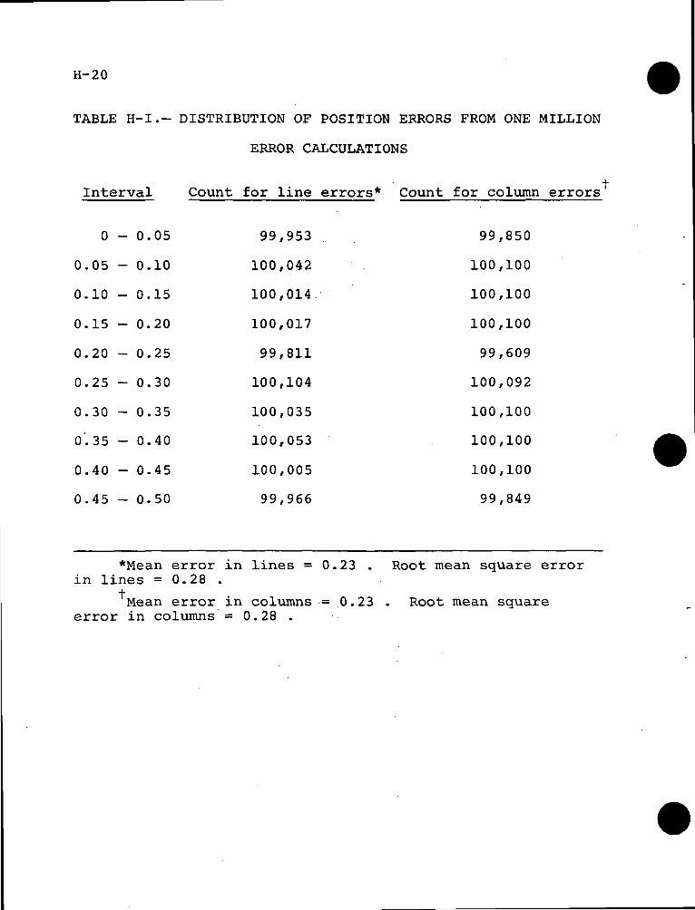
H-I DISTRIBUTION OF POSITION ERRORS FROM ONEMILLION ERROR CALCULATIONS . . . . . . . . . . H-20
K-I SUMMARY OF ERIM MSS PROCESSING PROCEDURES. . . K-43
K-II SUMMARY OF ERIM MSS PROCESSING PROGRAMS. . . . K-44
Page 23
XXV
FIGURES
Figure Page
1
2
3
4
5
6
7
8
9
10
11
12
13
14
15
16
Technology assessment data set, Maythrough September 1973
Map of ERTS-1 ground track positions,December 1972 through February 1973
Ground observations summary form
Optical depth observation form
Scanner data flow diagram
Diagram of organizational responsibilitiesfor the CITARS task
Diagram of organizational responsibilitieswithin EOD
Diagram of EOD key personnel assigned to .the CITARS task
Diagram of ERIM key personnel assigned tothe CITARS task
Diagram of LARS key personnel assigned tothe CITARS task
Milestone schedule of major task areas. . . .
Milestone schedule of detailed dataacquisitions
Milestone schedule of detailed dataprocessing activity
Milestone schedule of performancecomparisons
Milestone schedule of documentation
Schedule of EOD data processing requirementson ERIPS, Univac 1108, and the DAS
14
15
25
26
48
57
58
59
60
61
62
63
64
66
67
68
Page 24
XXVI
Figure Page
C-l Diagram showing existence of boundaryelements between fields where not indicatedby ground truth C-8
C-2 Diagram indicating no boundary elementswhere a boundary has been indicated by '
C-3
D-l
D-2
D-3
D-4
D-5
D-6
E-l
E-2
E-3
E-4
Example of field description codingsheets
Idealized sketch of Huntington County testsegment .
Idealized sketch of Shelby County testsegment
Idealized sketch of White County testsegment
Idealized sketch of Livingston County testsegment ; . . . . .
Idealized sketch of Fayette County test .segment
Idealized sketch of Lee County testsegment
Example of initial report for section 15 inLivingston County, Illinois
Example of annotated photobase to beincluded with initial report for section 15in Livingston County, Illinois
Example of interim or final report forsection 15 in Livingston County, Illinois. .
Example of annotated photobase to be
C-9
D-2
D-3
D-4
D-5
D-6
D-7
E-5
E-6
E-7
included with interim report for section 15in Livingston County, Illinois E-8
F-l Idealized sketch of Huntington County groundinvestigation tracts F-2
Page 25
^ XXVI1
Figure Page
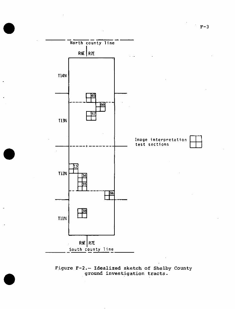
F-2 Idealized sketch of Shelby County groundinvestigation tracts F-3
F-3 Idealized sketch of White County groundinvestigation tracts F-4
F-4 Idealized sketch of Livingston County groundinvestigation tracts F-5
F-5 Idealized sketch of Fayette County groundinvestigation tracts F-6
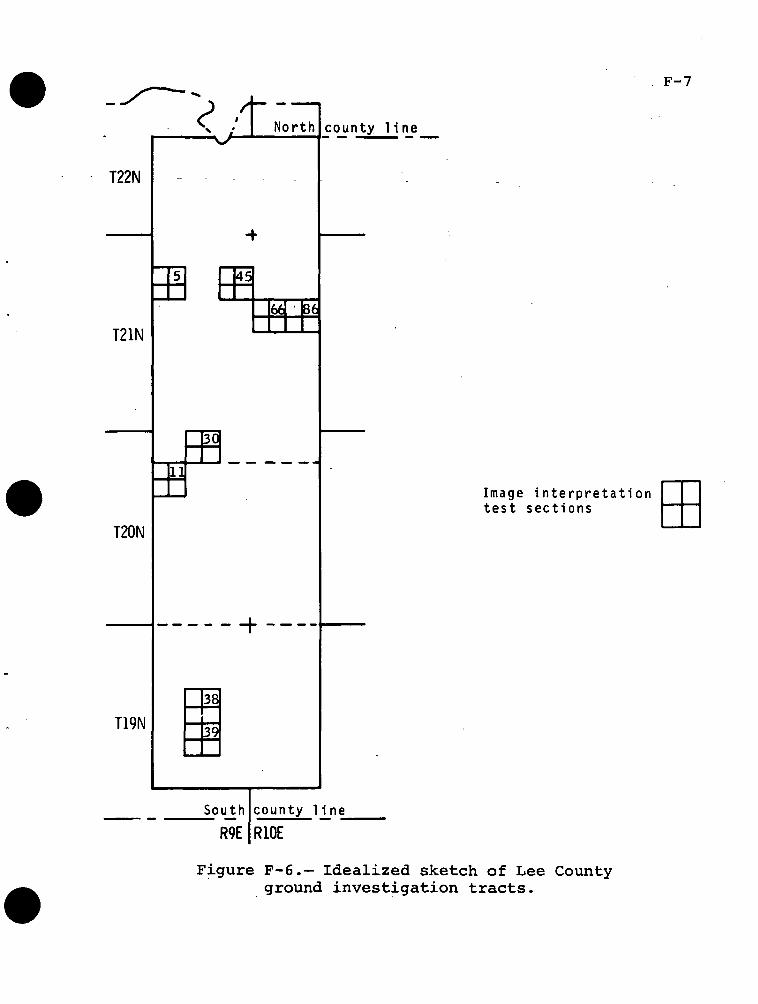
F-6 Idealized sketch of Lee County groundinvestigation tracts F-7
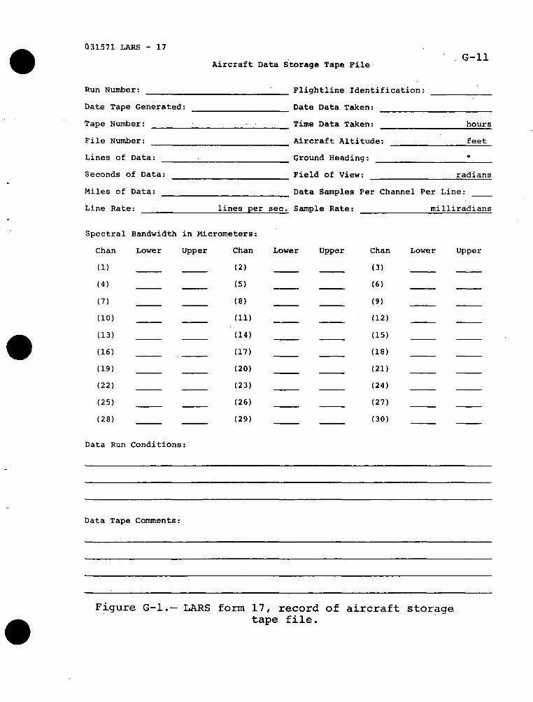
G-l LARS form 17, record of aircraft datastorage tape file G-ll
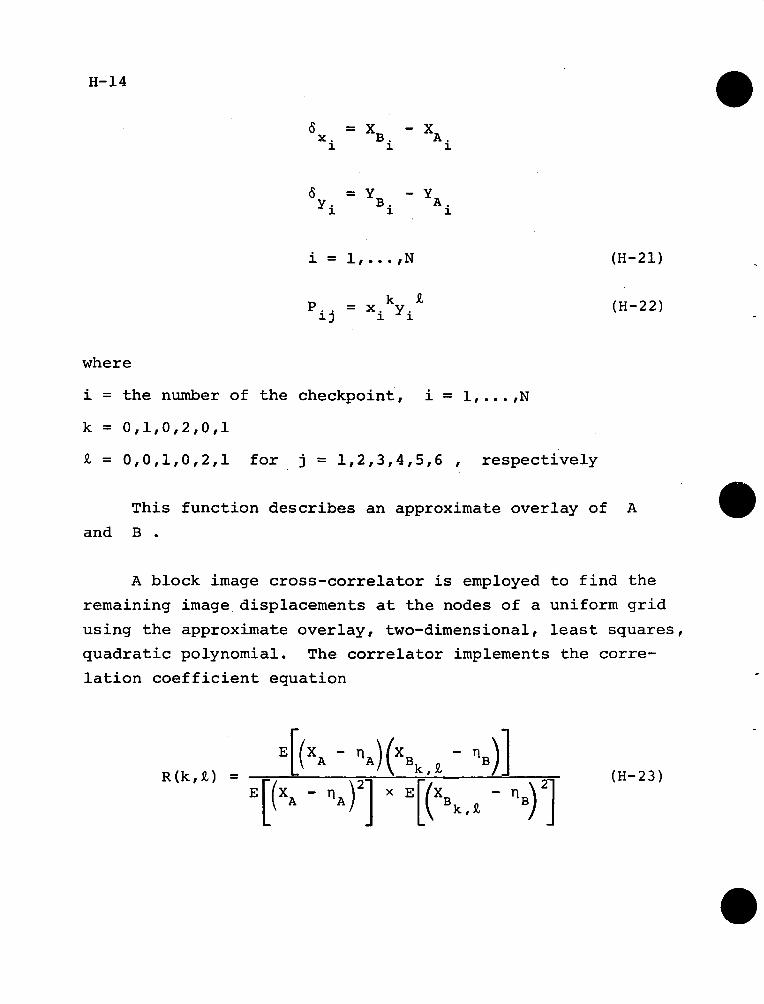
H-l ERTS MSS sample geometry H-21
H-2 Transformation illustration H-21
Page 26
1.0 INTRODUCTION
1.1 TASK DESCRIPTION
The objective of the Crop Identification Technology
Assessment for Remote Sensing (CITARS) will be the quanti-
fication of the crop identification performances (CIP's)
resulting from the remote identification of corn, soybeans,
and wheat, using automatic data processing (ADP) techniques.
The ADP techniques will be automatic in the sense that sub-
jective human interactions with the classification algorithms
will be minimized by specifying the steps required for an
analyst to convert a multispectral data tape to a classifi-
cation result. The capability demonstration will require:
1. The definition of specifications for well-defined ADP
techniques for making crop area inventories and quan-
titatively assessing the CIP of each area . - . : . , :
2. The definition of feasible aircraft and spacecraft
sensor platforms -
3. The definition of a sampling strategy optimally designed
for the demonstration project, the ADP procedure chosen,
and the platform used
4. The definition of a specific procedure for converting
the remotely sensed crop identification data to crop
area estimates in the demonstration region
The results of the CITARS task will be applied exten-
sively in the Large Area Crop Inventory Experiment (LACIE).
Page 27
1.2 BACKGROUND
1.2.1 Remote Sensing Data Processing Procedures
In May 1968, the Earth Resources Group was formed to
plan and direct remote sensing activities at the National
Aeronautics and Space Administration (NASA) Lyndon B. Johnson
Space Center (JSC). This group became the Earth Observations
Division (EOD) under the Science and Applications Directorate
(S&AD) of NASA/JSC in February of 1970. The EOD has directed
and participated in a team effort called Supporting Research
and Technology (SRT). An SRT team of which EOD is a member
is composed also of the Environmental Research Institute of
Michigan (ERIM) and the Laboratory for Applications of Remote
Sensing of Purdue University (LARS). The research and devel-
opment of techniques for converting remotely acquired spectral
data to usable resource information has been a major project
of this SRT team. At the same time, EOD has participated with
various, user agencies in defining the importance of certain
applications resource information to these agencies, their
requirements, and the capability of the technology base
developed by the SRT team to satisfy these requirements.
The primary products of the SRT techniques/applications
research and development activity are:
1. Remote sensing, photointerpretive, and ADP techniques
for the extraction of resource information from multi-
spectral imagery
2. A defined set of applications resource information
requirements, with defined priorities
Page 28
3. Knowledge, through testing and evaluating the techniques
and their applicability to the applications resource
requirements, of the feasibility of using existing tech-
niques to satisfy these requirements
4. A rational basis for decisions to discontinue or pursue
the further.development of techniques for particular
applications requirements
The ADP products have already been used to process some
data from the first Earth Resources Technology Satellite
(ERTS-1) and from high-altitude aircraft. The accuracy of
the crop identifications has convinced EOD and others in the
remote sensing community that the capability exists for
making crop inventories over large areas.
1.2.2 Large-Area Inventory Procedure
A procedure for making large-area inventories is well
established and has been successfully used by the Statistical
Reporting Service"(SRS) of the U.S. Department of Agricul-
ture (USDA) in its crop production estimate program. The
estimate procedure consists of three steps:
1. Strategic selection of areas to be intensively examined
for crop content
2. Identification of crops contained in the sampling areas
3. Measurement of the amount of each crop type within the
selected areas
Page 29
Errors arising as a result of this procedure are the
incorrect identification of crops, the inaccurate mensura-
tion or area measurement, and the sample error.
A similar procedure can be envisioned for a remote
sensing system, with the same error sources. The synoptic
acquisition capabilities of satellites and possibly high-
altitude aircraft can result in adequate coverage to reduce
significantly the occurrence of sample errors using conven-
tional techniques. Because crop identification errors
arising from the processing of multispectral scanner (MSS)'
data could lead to significant inaccuracies in crop inven-
tories, a careful evaluation is necessary before a large
area crop inventory is designed using existing remote sensing
technology.
Page 30
2.0 APPROACH
The remote sensing data will be collected by MSS onboard
satellites and high-altitude aircraft. The recently devel-
oped ADP procedures will then be used to classify the data
obtained within the six test areas of the U.S. Corn Belt.
The periodic acquisition of data will continue throughout
most of the growing seasons for corn, soybeans, and wheat.
Ground truth for these areas will be acquired con-
comitantly with the spacecraft and aircraft data by a
combination of field visits and the interpretation of
large-scale aircraft photographs. These data will identify
crops and other important agricultural conditions.
Classification results from the MSS data and ADP tech-
niques will be compared to the ground-truth data to estab-
lish the CIP's. These CIP's will be determined for several
periods during the growing season for both of the conditions
anticipated for an operational system:
1. Local recognition: Crop signatures for classifier
training will be obtained from the geographic region
in which the crops are identified.
2. Nonlocal recognition: Crop signatures for classifier
training will be obtained from a geographic region
other than the region in which the crops are identified.
Differences will be observed in the crop identification
capabilities of each ADP technique when aircraft and space-
craft data are processed. These will be analyzed and
examined for the situations described in conditions 1 and 2.
Page 31
Upon establishment of the CIP for each type of data
processing technique in the two basic remote sensing situa-
tions described, differences in the performances of these
types of processing techniques for crop identification- will
be established. The signature extension capability also
will be ascertained .for each ADP technique by determining
whether CIP's for local recognition differ significantly
from CIP's for nonlocal recognition. Finally, the perform-
ances of the ADP techniques in each of the remote sensing
situations discussed will be compared and examined for
significant differences.
To specify the well-defined ADP techniques for the
capability demonstration, the CIP's of these techniques,
and the agricultural and meteorological conditions associated
with these performances, the following questions will have
to be answered:
1. How do corn, soybean, and wheat identifications vary
with time during the growing season?
2. How do CIP's vary among different geographic locations
having different soils, weather, management practices,
crop distributions, and field sizes?
3. Can statistics acquired from one time or location be
used to identify crops at other times and/or locations?
4. How much variation in CIP is observed when different
data analysis techniques are used?
5. Does the use of multitemporal data increase CIP?
6. Does the use of radiometric preprocessing extend the
use of training statistics and/or increase CIP?
Page 32
7. How much deviation in CIP occurs when the selection
of training sets varies?
8. Are similar CIP results obtainable from spacecraft and
aircraft data acquisition systems?
After the CIP for each of these questions is estimated,
analysts will determine whether any observed differences
are significant.
Page 33
3.0 DETERMINATION OF TEST AREAS
3.1 TEST SITES
The CITARS test sites have been selected by the
Agricultural Stabilization and Conservation Service (ASCS)
of the USDA, ERIM, EOD, and LARS to satisfy the following
requirements:
1. To include the range of climatic and agricultural
conditions characteristic of the U.S. Corn Belt
2. To maximize the probability of obtaining repeated,
cloud-free coverage by the spacecraft MSS
3. To minimize the statistical bias attributable to the
process of site selection
4. To conserve the aircraft resources required to obtain
MSS data and aerial photographs
Repeated coverage by the ERTS-1 MSS was assured by
limiting site selection to the four overlap zones of the
five ERTS-1 passes over Indiana and Illinois (passes L, M,
N, 0, and P). The agricultural records of these states
were used to stratify the counties within each zone with
respect to such factors as climate, distribution of crops,
crop productivity, soil type, variability of soil color,
and topography. The following results were obtained.
Page 34
10
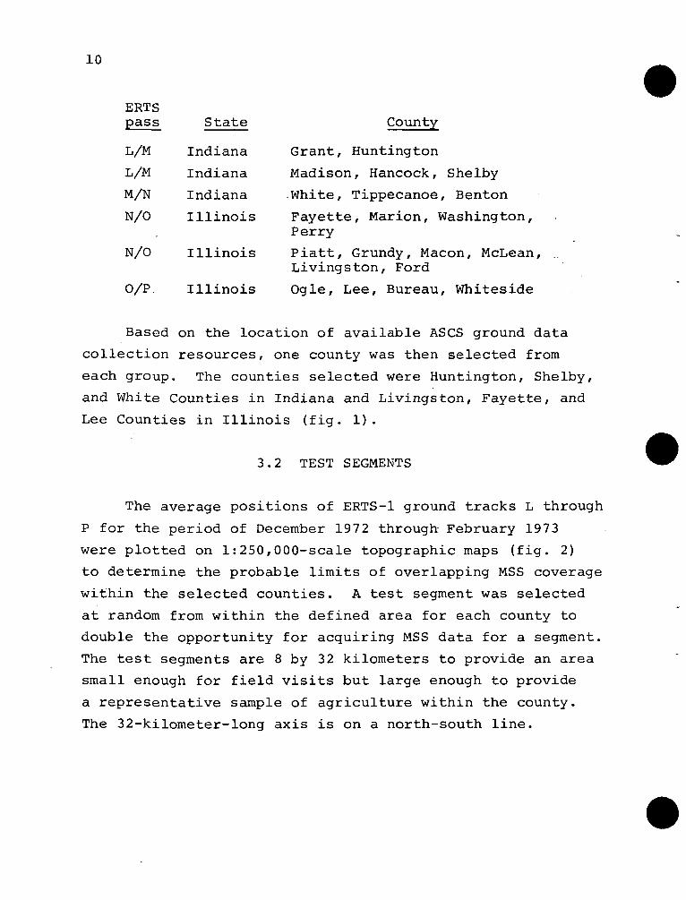
ERTSpasss State County
L/M Indiana Grant, Huntington
L/M Indiana Madison, Hancock, Shelby
M/N Indiana .White, Tippecanoe, Benton
N/O Illinois Fayette, Marion, Washington,Perry
N/O Illinois Piatt, Grundy, Macon, McLean, ..Livingston, Ford
O/P Illinois Ogle, Lee, Bureau, Whiteside
Based on the location of available ASCS ground data
collection resources, one county was then selected from
each group. The counties selected were Huntington, Shelby,
and White Counties in Indiana and Livingston, Fayette, and
Lee Counties in Illinois (fig. 1).
3.2 TEST SEGMENTS
The average positions of ERTS-1 ground tracks L through
P for the period of December 1972 through February 1973
were plotted on 1:250,000-scale topographic maps (fig. 2)
to determine the probable limits of overlapping MSS coverage
within the selected counties. A test segment was selected
at random from within the defined area for each county to
double the opportunity for acquiring MSS data for a segment.
The test segments are 8 by 32 kilometers to provide an area
small enough for field visits but large enough to provide
a representative sample of agriculture within the county.
The 32-kilometer-long axis is on a north-south line.
Page 35
11
3.3 SECTIONS
3.3.1 Quarter Sections
Each 8- by 32-kilometer segment was divided into five
columns and four rows of 1.6- by 8-kilometer sections.
One quarter-section tract was selected at random within
each of the 20 sections. The small-scale imagery (scale:
1 inch = 1.6 kilometers) of each quarter section was
examined. If water, trees, urban development, air, fields,
or other readily identifiable, nonagricultural-use features
occupied more than 10 percent of the quarter section (20 per-
cent in Huntington County where small wooded areas are
common), a replacement tract was selected. The quarter
sections will be used for field visits by the ASCS to
obtain ground-truth data. The procedures for selecting
sections and quarter sections are set out in greater detail
in appendix A.
3.3.2 Test Sections
One additional section, disjointed from each quarter
section, was then randomly chosen from each of the 20 sec-
tions. The ground-cover classes in these sections will be
identified by photointerpretation and will serve as test
sections for the evaluation of CIP. Appendix D shows the
distribution of quarter-section and test-section tracts
selected for ground investigation in each county.
3.4 ,FIELDS
Data for the CITARS experiment have been collected
from training fields, test fields, and pilot fields.
Page 36
12
(See appendix B for training, pilot, and test field selection
procedures.)
3.4.1 Training Fields
Ten quarter sections will be selected at random from
the 20 ASCS quarter sections in each segment. From the
10 quarter sections selected, all crop fields large enough
to be accurately located in the scanner imagery will be
available for training the classifier.
Training areas for nonagricultural types not present
in the 10 quarter sections, such as water bodies, forests,
towns, and airports, will be selected arbitrarily from the
base photography. If present in the segment, 10 areas of
nonagricultural type will be selected, and their coordinates
will be located in the scanner imagery.
In order to compare results, all classifications will
be performed using these training fields. No additional
fields may be selected for training during the analysis.
3.4.2 Pilot and Test Fields
All the fields in the 20 photointerpreted sections will
be designated as test fields unless an estimate of classi-
fication errors is required. Then all the fields in one-
half of the 20 photointerpreted sections will be designated
as pilot fields, and the remaining fields will serve as test
fields. The pilot fields will be used to determine the
feasibility of correcting for the bias in the classified
crop proportions resulting from classification errors.
Page 37
13
Errors will be estimated in these fields, and the correction
determined from these estimates will be applied to the test
field.classification results. (Appendix C gives the proce-
dures for locating test field boundaries.)
Data gathered from the test fields will be classified
by ADP techniques and used, along with other specified data,
to determine CIP's.
Page 38
14
ERTS-lpasses:
One segment:8 x 32 km25,856 hectares(64,640 acres)
One section:-256 hectares(640 acres)
ERTS-loverlap
Study Area Counties:
Indiana
1 . Hunti ngton 42. Shelby 5
I l l i n o i s
Li vi ngstonFayetteLee
Data Acquisition Periods:
0 - 5/21-25/73 IV - 8/01-05/73
6/08-12/73I
II - 6 / 2 6 - 3 0 / 7 3II I - 7 / 1 4 - 1 8 / 7 3
3. W h i t e 6
Ground Truth:
A S C S - 20 quarter sec t i ons ( w h i t e ) each ERTS- l pass
Photo in terpreta t ion - 20 sec t i ons ( b l a c k ) each ERTS- l pass
V - 8 /19-23/73VI - 9 / 0 6 - 1 0 / 7 3
V I I - 9 / 2 4 - 2 8 / 7 3
Figure 1.— Technology assessment data set,May through September 1973.
Page 39
15
OSH
X!4J
S-i(U
u0)Q
O-H-P•H •w nO r-
u >,rti S-lM (0-P 3
C 0)d faOS-ltr>
ICflEHtfW
ai•
(N
Q)
Cn•H
Page 40
17
4.0 DATA ACQUISITION
-; Several types of - data are required to meet the task
objectives:
1. Scanner data from spacecraft and aircraft platforms
2. Aircraft photography from low or intermediate altitudes
(These data will be used for crop identification exten-
sions by identifying selected agricultural conditions
and by measuring areas and delineating fields in.the
scanner data.) ,~
3. Ground investigations to provide crop identifications
and condition and progress reports on meteorological
^conditions throughout the period-of the experiment
4. High-altitude metric photography for ground-truth
annotation and couritywide coverage .,
The ERTS-1 MSS data are acquired at 18-day intervals
along each ground track. Both the ground observations and
the aircraft support flights are coordinated with ERTS-1 over-
flights. The dates of overflights during ERTS-1 cycles 16
through 25 are presented in table I. Data acquisition
periods have been identified as 0 through VIII, but the
acquisition periods of primary interest for ADP processing
are periods II through VI (fig. 1). The ASCS field visits
and low-altitude aircraft photography were mandatory during
periods II through VI. Because of the uncertainties involved
in the acquisition of these data, periods I through VII will
be analyzed if necessary. The support data schedules could
be made more flexible by taking advantage of improved weather
conditions.
Page 41
18
4.1 SPACECRAFT SCANNER DATA
Both the MSS on the ERTS-1 and the MSS on Skylab should
be operational during the data-collection phase of this
experiment.
4.1.1 ERTS-1
The scanner mounted on the ERTS-1 collected four-channel
data covering a strip 280 kilometers wide on each pass across
the United States. Orbital parameters of the ERTS-1 were
designed to repeat the coverage along each ground track at
18-day intervals. Because its orbit is Sun-synchronous,
the ERTS-1 views an area with similar conditions of illumi-
nation on every pass, at approximately 10 a.m. local stand-
ard time. This provides an adequate record of temporal
changes in the spectral responses of developing crops.
Because weather summaries indicate a high probability
of greater than 30 percent cloud cover in this region during
the summer months, EOD has acquired bulk, MSS, nine-track,
computer-compatible tapes (CCT's) with 314.9 bits/centimeter
for MSS frames that include coverage of the test segments.
The MSS frames with reported cloud coverage of 70 percent or
less were on standing order for ERTS-1 cycles 16 through 24.
Frames reported to include greater than 70 percent cloud
cover will be screened as microfilm copy arrives. If the
test segment (only 1 percent of the frame area) is signifi-
cantly free of clouds, all CCT coverage of the frame will
be ordered. Tapes for frames that provide acceptable
coverage of a test segment will be duplicated by JSC for
Page 42
19
shipment to LARS. The loss of data from the study area
during one 18-day cycle because of cloud cover or malfunc-
tion would impair the documentation of temporal changes in
crops.
4.1.2 Skylab
The MSS mounted on Skylab collected data over one or
more of the test segments during August and September of
1973 for comparison with the ERTS-1 data. Skylab retraced
each ground track at intervals of 118 hours; the spacecraft
crossed a point on the ground track 12 hours earlier in the
day on each successive overflight. The MSS was nominally
oriented with the Z-axis to local vertical orientation.
4.2 AIRCRAFT SCANNER DATA
, - - , . ' . ' • '
Data from a state-of-the-art, aircraft-mounted MSS are
required throughout the period of the experiment to monitor
the changes in spectral responses associated with the full; j" i ' • '• .
cycle of crop development. An aircraft-mounted MSS that
covers'atmospheric windows in the reflective infrared and
thermal infrared regions would be desirable. The inclusion
of thermal infrared scanner data in this assessment would
increase the reliability of projecting the results of data
interpretations from spacecraft scanners that are sensitive
to thermal infrared radiation; that is, those on Skylab and
those that will be on the second Earth Resources Technology
Satellite (ERTS-B).
Page 43
20
Data from two other state-of-the-art scanners were
required from June through September 1973. These scanners
were the modular 11-channel scanner (M S) developed by The
Bendix Corporation and the modular 12-channel scanner (M-7)
developed by ERIM. Data from the M2S will be the prime air-
craft scanner data source for comparison with the ERTS-1 MSS
performance. The CIP obtained by analysis of data from the
M-7 scanner will be compared with the M S and the MSS CIP's
to determine the utility of the 1.5 through 2.6 bands (not
available on the M2S).
2Six data acquisition missions were flown with the M S
and two with the M-7. The schedules for these missions were
coordinated as closely as possible with ERTS-1 cycles 19
through 24. Aircraft coverage within 4 days of the last
day of each ERTS-1 data acquisition period, with less than
10 percent cloud cover and a Sun angle greater than 40° was
highly desirable. Contingency aircraft data acquired within
5 to 8 days after the last day of the ERTS data acquisition
period will be acceptable with less than 30 percent cloud
cover and a Sun angle greater than 30°. Because scan-angle
effects severely degrade recognition accuracy, no more than
50° of the total field of view of scanner data will be proc-
essed. Since the aircraft flight lines were required to be
parallel to the centerline of the 20-mile length of the seg-
ment, two flight lines provided complete coverage of the
segment.
4.3 AIRCRAFT PHOTOGRAPHIC DATA
Because a more accurate estimate of the CIP for each
ADP technique could be obtained if a larger field sample
than that collected by ground investigation were available
Page 44
21
from each segment, 20 additional sections in each segment
will be collected. With these data, skilled photointer-
preters will delineate training and test fields in the
scanner data and extend crop identifications from fields
observed on the ground to fields in nearby sections. Agri-
cultural conditions such as soil variability, row spacing
and orientation, and crop uniformity can be readily evaluated,
and temporal changes can be documented. Areas measured on the
photographs will permit accurate determination of the pro-
portions of crops in selected groups of contiguous fields.
High-altitude (3,000 to 4,500 meters), color infrared
photography covering the six counties was obtained from the
RB-57 aircraft with the RC-8 camera, using Kodak 2443 film.
This coverage was requested for three periods in 1973:
1. June 8-30 (June 26-30 was considered very favorable.)
2. July 8-25 (July 14-18 was considered very favorable.)
3. August 1-23 (August 19-23 was considered very favorable.)
A Fairchild 224 camera (150-millimeter focal length,
225-millimeter format, Kodak 2443 film) installed on a
Bendix Queen Aire will provide an image of adequate resolu-
tion from altitudes of 4,500 meters or less. The photo-
graphic missions should be scheduled coincidentally with or
following the overflights of ERTS-1 cycles 18 through 23 so
that the imagery can be used to investigate any anomalies
(such as those caused by flooded fields or hail-damaged
crops) that were present in the ADP identifications. Cloud
cover of less than 10 percent is highly desirable; less than
30 percent is mandatory.
Page 45
22
Metric photography for mensuration was mandatory for
the missions flown in late June and late August. This
photography was acquired with the NASA Zeiss metric camera"i
installed aboard the Michigan C-46 aircraft at ERIM.
4.4 GROUND INVESTIGATIONS
Ground investigations by experienced ASCS field
personnel in the six counties will provide the. control
required for the technology assessment. Two types of data
will be collected: agricultural information and atmos-
pheric, optical depth information.
4.4.1 Agricultural Data
Agricultural observations in the 20 quarter sections
in each segment are planned to coincide approximately with
the ERTS-1 overflights (every 18 days). A plus or minus
variance of 24 to 48 hours because of weather or weekend
schedules is acceptable. On the first visit to each quarter-
section tract, ASCS personnel will mark the boundaries of
each field on a base photograph and assign an identification
number to each area. Then the crop or land use will be
identified, and data concerning cultural practices and crop
conditions will be recorded. This will be repeated on sub-
sequent visits, and any changes that occurred since the
preceding visit will be noted. The Ground Observations
Summary Form (JSC form 1570A) will be used to simplify
uniform reporting of ground investigation data (fig. 3).
The crop identifications are required to train the photo-
interpreters and to test the classification results.
Page 46
23
Periodic reports of the agricultural conditions in fields
used for training and testing will be used to supply the
data needed to evaluate the probable causes of misclassified
points.
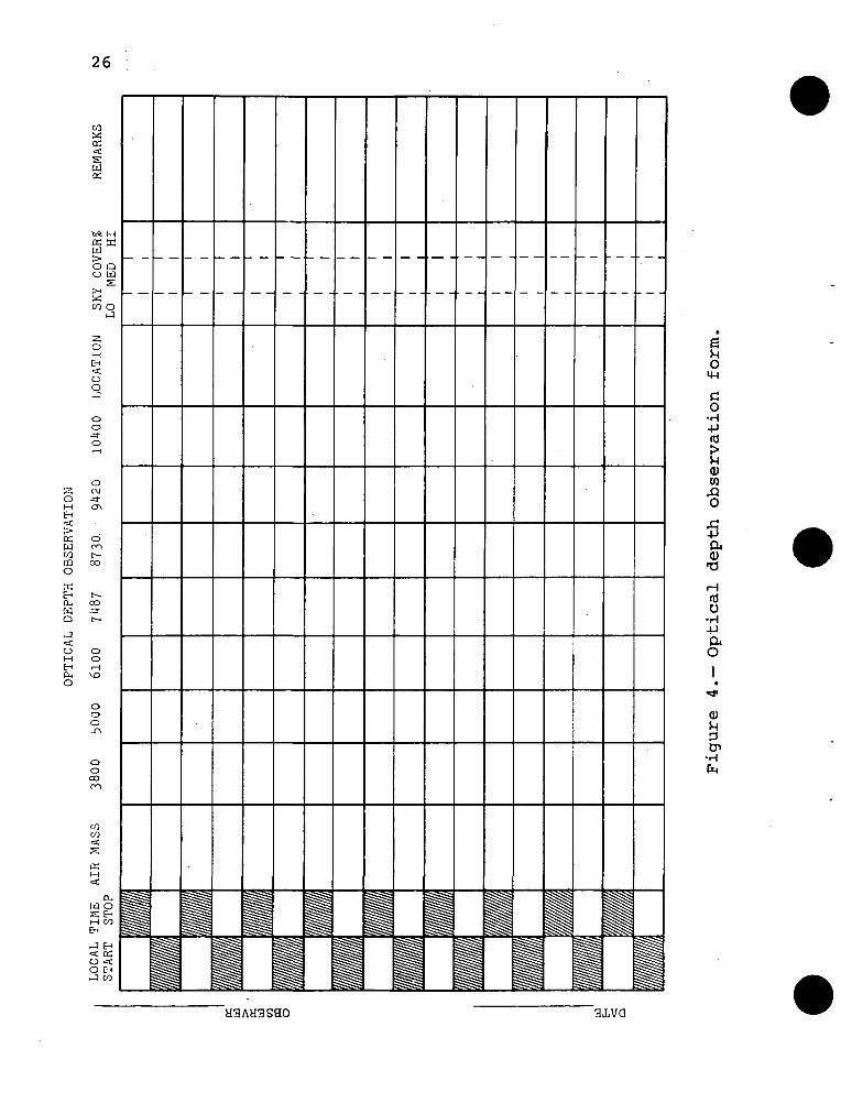
4.4.2 Atmospheric Optical Depth Data
Solar radiation will be measured to obtain valuable
information about the atmospheric layer between the space-
craft and the surface. A seven-channel solar spectropho-
tometer built at JSC has been issued to each participating
county for this purpose. Observations will be recorded on
the form entitled "Optical Depth Observation" (fig. 4). The
ASCS crews were requested to take five sets of readings on
the day of each scheduled ERTS-1 overflight:
1. One reading in early morning, anywhere in the county
2. Three readings between 9:00 and 10:00 a.m. local time:
one from a station in the northern quarter, one from the
southern quarter, and one from the middle of the segment
(in any order)
3. One reading near solar noon, anywhere in the county
The second group of readings had higher priority than
the first or third since they related directly to potential
correction of the ERTS-1 MSS data. Timing was critical,
inasmuch as weather or scheduling problems could prohibit
the taking of readings at scheduled times, thus causing the
loss of data.
Page 47
24
TABLE I.— ERTS-1 COVERAGE SCHEDULE FOR TEST SEGMENTS
ERTS-1cycle
16
17
18
19
20
21
22
23
24
25
Month
May
May
June
June
July
August
August
September
September
October
Period
0
I
II
III
IV
V.
VI
VII
VIII
i Date of overflight along track
L
3
21
8
26
14
1
19
6
24
12
M
4
22
9
27
15
2
20
7
25
13
N
5
23
10
28
16
3
21
8
26
14
O
6
24
11
29
17
4
22
9
27
15
P
7
25
12
30
18
5
23
10
28
16
Counties covered:L/M M/N N/0
Huntingtonand ShelbyCounties,Indiana
0/P^ -
\White Livingston Lee County,County, and Fayette IllinoisIndiana Counties,
Illinois
Page 48
25
^*o
1
ai^
oj_>
Obs
erva
^
\r>
CQJ QJ
E UO >,U u
O C
1 >.
o i-UJ
QJ
<o
•— QJ3 -0
•— U QJ i- ~O•r- QJ QJ QJ JZO >v i/> QJ 4-J 4-> >iul •— 4-> C 3 4->
JC >* C *Q O QJ
i- QJ 5 •— CX O> C03 i- QJ O QJ QJ QJco u_ z :> o: oe 01.— <NJ co *3- in ^ E
c
•M 4-> C
T3 O. O- Ecm C4-» TO O *+- •—in QJ i- U
C 0. >C 5 O--»- Or^ OT- 1-J= J- .* 4J CK- Q 00 00 •«-
1 1 1 1f— «— 1— *— •*•>
(0
4-*V)
QJ 0)
03 t-•— (0
T3 -r- JCQJ 01
in i- QJd> -o o •»-> ••
*O > ' QJ "O **-**- W»
4-* tO CT fO 2 "O O
QJ •.- ,— i- a. QJ «o> 4-> M o "O Q.-— <dUJ (O C QJ -r— JC ••—T* O- CD Q 2 (J l~~ ini i i i i i i m^acMCocvjcuoocsj L.
oo
oQJ
"O UQJ QJ QJ •— QJo» <u »A **- a> -•E X Q QJ QJ IO QJ10 QJ T3 C7» E i-
"O >i </» m 2 *** 3
J= E QJ "O C 4J -r-CT> QJ 4-> -t- -r- U O3 t. C I- •— 01 QJ ZO 4-» IO 4-» -r- "O Wt. x *— 3 m o c QJa uj a. ;= :c _i •— i ul l l l 1 i l ro
PO ro n ro ro PO co i-3
CO
QJ
10
C
C 4->
in c ••-i- O OJ 4J i-Q z: 3 oo «— ••
Mr— CVJ CO - UTJ QJ r-^,«r^^ ij-n
s1/1U-lwll/l<£
CS
3oZT3:(_>UJ
a:O
gO-O-
S-OJ
-oc:
oo
*^
«
o0101(O
LO
0
D
'ai
co
re ens-
t/i
o
J_01> ooo
<->
^T3 r-~
-*
i ^o
4-1
3 "^
2-
^
1
a.O f*lS--^
+-> CM
3 ^
aioo•acoCJ
o
ua>L-
O
I
Lf)
o
11
UJ
l/>>_
ct1—
Q.
§
CO
cE3
oo
*£>
CE3
"oCJ
/I
UJ
»-
/I
3
ILJ
CX
*5 ** »« O*« O O O Oin CVJU") CO ^
1 1 1 1 1o mo o o
co m co
i i i i i
O •— Cg CO F
(/> UJ UJ S-3 oo z: 30 CO 3E 0
1 t C
Z Z Ul S OO O
1 1 1 1 1 1
o •— oo ro «3- LO
c
§ 5.Q.QJ 4-> t— O
l-O QJ -— i-CO QJ -O
__"9 __ -**O C Q. O CT> QJO -r- O- C >
»— E 3S ~f- TJJD O >— QJ C QJQJ O ^ -M t. ^i- f— T3 UJ 3i. CO UJ *J h—
•— oo ro «* in
QJ T3t/l QJin r— QJm QJ L.
4-* in 3QJ in 4->
0. h- Z
r- oo ro
0^~
>.
cn-o c QJQJ •— i-
4J -O C 3o *o u. •*->O QJ 3 rtj
LO 3: t— 2: i-Q>
F— co ro ^- o
QJ
3
<o
VO
co
exI-u(/Iai
T3
o3o•M
oatco
Page 49
26
OSWCOCQO
EHPHwQ
OMEHCMO
WK
fc«. MK MW
O QO W
S>H«
CO O
2;oMEH<Oo
oo
oCM
Ornc—CO
oo
oooLTV
OO00
COco
IX,Id OS EHM COEH
J EH< OSo <O EHJ CO
Go•H-P
(1)CO.QO
(1)•o
O-HJ-l
0)
tr>•Hfa
H3AH3S90 3J.VQ
Page 50
27
5.0 DATA HANDLING
To accomplish the CITARS objectives., an experiment
must be designed to:
1. Accurately estimate the CIP
2. Determine whether the differences in CIP's for various
conditions are significant
Each CIP will be established on the basis of a specific
treatment combination characterized by the following factors:
1. Platform-sensor combination:
a. ERTS-1 MSS
2b. Aircraft M S
c. Aircraft M-7
d. Aircraft multispectral data system (MSDS)
e. Earth Resources Experiment Package (EREP) MSS
2. ADP technique: The 11 techniques are defined in
section 5.3.2.
3. Data acquisition period: The six periods of data
acquisition are set out in section 4.0. It is antici-
pated that the levels in this factor will differ when
using multitemporal ADP techniques; for example, if
data from three passes are used for the analysis, there
are 10 possible ways of combining the six data acquisi-
tion periods.
4. Location: The six test sites are discussed in section 3.0.
Page 51
28
5. Training recognition: Many possible levels exist,
but they will be characterized as:
a. Local recognition
b. Nonlocal recognition
Each treatment combination will have an associated
CIP that will be quantified in three ways:
1.. The classification performance matrix will be used to
determine errors of omission and commission. It will
be established by comparing the ADP classification with
the ground and photointerpretive identifications of
about 5,120 hectares within each data segment. The
probability for correct classification of corn, soybeans,
wheat, and "other" for a particular test field set will
be defined as the frequency with which test field pixels
of a particular class are classified correctly. The
error of commission between two classes will be defined
as the frequency with which an ADP identification of one
of the classes is determined from ground truth to have
been actually a pixel from the other class. For a four-
class data set, this procedure will define a 4-by-4 error
matrix.
2. The proportion classification error vector will be
established by comparing the proportions of corn, soy-
beans, wheat, and "other" (determined from the ADP
technique) to those proportions determined from photo-
interpretation and ground truth (sections 4.3 and 4.4).
3. A proportion error vector will be estimated for each
treatment based on a proportion vector corrected for
bias. The proportion of each crop type in the sections
Page 52
29
within each segment will be established by mensuration
of the photography. The result will be compared with
the proportions established by the ADP techniques to
determine the ADP proportion error vector. In addition,
several methods have been proposed for correcting the
remote sensing estimates of the crop proportions for
bias. Each of these methods will require an estimate
of the bias, which is obtained by examining the classi-
fication performance in pilot fields.
5.1 AIRCRAFT PHOTOGRAPHIC DATA
Aircraft photography will be processed at JSC. Selected
frames required for base maps will be printed at the appro-
priate scale in the required quantities. The JSC interpreters
will study, as a minimum, the photographs exposed during the
June, July, August, and early September missions before
reporting final conclusions. Field boundaries of the areas
to be provided with supplemental identifications and some pre-
liminary decisions will be available in August. (Appendix E
sets out the procedures for photointerpretation.)
Image interpretation data will include:
1. Outlines of fields to be identified on the base photograph
2. Interpreted identifications of crops in specific fields
3. Determination of the proportions of areas occupied by
corn, soybeans, wheat, and "other" in a group of con-
tiguous fields occupying multiple-section blocks
4. Documentation of changes occurring within each field
Page 53
30
The accuracy of photointerpretive crop identification
procedures will be determined by the test procedure described
in appendix B. If the test indicates errors in the photo-
interpretation field identifications, the source and nature
of the photointerpretive errors will be ascertained, and the
effects of these errors on the estimates of the ADP CIP will
be assessed.
5.2 GROUND INVESTIGATION DATA
Ground investigation data will be shipped from the
ASCS offices to JSC, where they will be assembled. Copies
of the crop identification and agricultural practice data
for each segment will be transmitted to ERIM and LARS as
the ERTS-1 tapes become available. A modified copy of the
crop identification data will be distributed to the EOD
Image Interpretation Team. Selected quarter-section blocks
that have been investigated by the ASCS teams will be con-
cealed from the interpreters as a test set to be used in
evaluating the accuracy of identifications from aircraft
photography. Great care will be taken to ensure the removal
of data for these fields from each set of ground-truth data
distributed to the image interpreters. (Appendix F outlines
the procedure for testing photointerpretation accuracy.)
5.3 MSS DATA
5.3.1 Data Preparation
Specific procedures will be followed in reformatting
the spacecraft and aircraft MSS data and in identifying the
section, quarter section, and specific field and field types
Page 54
31
from which the data were taken. Each institution involved
will use common training and test field boundaries and dupli-
cate spacecraft and aircraft scanner tapes to permit more
meaningful "performance comparisons and to eliminate the need-
less duplication of tasks and resources at each institution.
To implement this philosophy, LARS will reformat the
ERTS-1 and M-7 scanner tapes into the format of a classifi-
cation program developed at LARS (LARSYS 3). Modular MSS
data will be accepted at JSC and screened and reformatted.9
as necessary. The EOD will reformat the M S and MSDS pulse-
code modulated (PCM) tapes into LARSYS 3 format. Duplicate
tapes will be shipped to ERIM and LARS, as required. The
M-7 data will be screened by ERIM, and duplicate copies of
the analog tapes will be sent to LARS and EOD. LARS will
then select the field boundaries en all the tapes for use
at each institution. (See fig. 5 for data flow, appendix G
for data screening and evaluation procedures, and appendix H
for data preparation procedures.)
5.3.1.1 ERTS-1 data.- ERTS-1 bulk data tapes will be
received from the Goddard Space Flight.Center (GSFC) by EOD
personnel for duplication at JSC. During the duplicating
activity, the tapes will be visually screened on a cathode-
ray tube (CRT) color display, using various combinations of
three of the four bands to obtain and record the following:
1. Quick-look band-by-band data quality
2. General location of the segment by line and column count
and extent of coverage within the CCT
3. Degree of cloud coverage over the segment
Page 55
32
Of the two data passes over each segment, the one
acquired during minimum cloud cover will'be selected* for'"
local recognition. If cloud cover is equal for the two
passes, the data acquired most temporally coincident with
the ASCS field visit will be chosen for local recognition
processing.
The duplicated tapes will be forwarded to LARS for sub-
sequent reformatting and field boundary definition. The LARS
will then send duplicate copies and field coordinates of the
reformatted tapes to EOD and ERIM for data analysis processing.
5.3.1.2 EREP scanner data.- Some EREP MSS data may
have been acquired over the technology assessment segments.
If so, these data will be analyzed for CIP and compared with
CIP's obtained in other trials. The exact procedures used
to accomplish this task will hot be defined until the nature
and quality of these data are known.
5.3.1.3 Aircraft scanner data (M2S, M-7, MSDS).- The
data from each aircraft scanner pass over each segment will
be examined for quality (appendix G). If found acceptable,
the data will be reformatted to LARSYS 3 format, and the
training and test field boundaries will be selected at LARS.
Copies of the field coordinates for each aircraft tape will
be sent by LARS to EOD and ERIM to ensure that each institu-
tion is using identical test and training data and to elimi-
nate the needless duplication of the resources required to
select field boundaries.
Page 56
33
5.3.2 Data Processing
Each of the 11 ADP techniques will be used to process
reformatted duplicate data (discussed in section 5.3.1 and
in appendix H) for each scanner data source. Each technique
consists of a computer-implemented software system and a
method or procedure by which MSS data can be converted into
ground-cover class identification information on a pixel-by-
pixel basis.
The CIP of ADP techniques can be sensitive to the
manner in which the classifier is trained, the types of
MSS input data (for example, preprocessed, multitemporal),
the spectral bands which are used for recognition, and so
forth. Most of the.existing procedures for the use of very
generalized analysis algorithms require decisions on the
part of the analyst; these decisions also can significantly
affect the classification performance obtained.
A quantitative evaluation and subsequent comparison of
the CIP's of the ADP techniques will be most meaningful if
the procedures used to obtain the classification results are
well defined and repeatable. Therefore, each of the ADP
techniques evaluated in this task will be documented in
detail (appendix I), and the documented procedures will be
observed rigidly to reduce variations in the classification
repeatability of an ADP technique. Any proposed deviation
from these procedures must have the prior approval of the
Technical Advisory Team described in section 6.0.
Each ADP technique to be evaluated is described in
general terms in the following discussion (for more detail,
see appendixes J, K, and L). The techniques are grouped
Page 57
34
into three categories: standard, preprocessing for signature
extension, and processing for multitemporal and unresolved
objects. A code is used to distinguish each technique with
regard to:
1. The data source: ERTS or aircraft
2. The Institution: EOD, ERIM, or LARS
3. The processing technique: standard processing (SP), pre-
processing and standard processing (PSP) , multitemporal
processing (MSP), or unresolved objects processing (UP)
5.3.2.1 Standard ADP techniques.- These techniques
use either Gaussian maximum likelihood classifiers or classi-
fiers using a linear decision rule. They classify data
which have not been radiometrically preprocessed or acquired
multitemperally.
5.3.2.1.1 ERTS-LARS-SP1: A combination of manual and
automatic clustering techniques is used to identify spectral
subclasses, which are assumed to have equal a priori proba-
bilities. These subclasses are used to compute the training
statistics required by the maximum likelihood classification
algorithm. This algorithm is a standard part of the LARSYS 3
program.
5.3.2.1.2 ERTS-LARS-SP2: This technique is similar
to ERTS-LARS-SP1, except that SP2 includes a procedure for
estimating the relative proportions of the object crops
from field data and a procedure and software for using these
proportion estimates as a priori probabilities in the decision
algorithm. In the early portion of the technology assessment
effort, LARS will conduct statistical tests to determine the
best of SP1 and SP2 with respect to CIP. If SP2 proves to
Page 58
35
be more accurate, it may replace SPl for the remainder of
the assessment.
5.3.2.1.3 Aircraft-LARS-SP1/SP2: These techniques
differ from ERTS-LARS-SP1/SP2 in only one respect: Feature
selection will be used to select the best subset of the
available spectral channels based on the LARSYS 3 separa-
bility processor.
5.3.2.1.4 ERTS-ERIM-SP1: A classification algorithm
is used to apply best linear decision boundaries between
classes, as opposed to the quadratic decision boundaries
applied by the other conventional algorithms to be tested.
Each major crop will be represented by a single multivariate
Gaussian distribution function (selected by choice for this
proceduralized technique). Additional signatures will be
determined only for those "other" classes of training data
that are likely to be misclassified as one of the major
crops.
5.3.2.1.5 ERTS-ERIM-SP2: A maximum likelihood classi-
fier (quadratic rule) is used in place of the best linear
decision rule. Otherwise, this technique is similar to
ERTS-ERIM-SP1.
5.3.2.1.6 ERTS-EOD-SP1: The training field data for
corn, soybeans, and wheat will be preprocessed by independent
runs of the EOD Iterative Self-Organizing Clustering System
(ISOCLS) on the Earth Resources Interactive Processing System
(ERIPS) at JSC. The ISOCLS routine will generate class and,
if necessary, subclass statistics; that is, corn 1, corn 2,
and corn 3. The training fields for "other" will then be
Page 59
36
submitted to the same clustering scheme to generate class and
subclass statistics for all "other." The training field, test
field, and test section data will then be classified using the
Gaussian maximum likelihood classification algorithm on ERIPS
to process the statistics previously generated with the clus-
tering process.
5.3.2.2 ADP techniques with preprocessing for signa-
ture extension.- Before nonlocal recognition is accomplished,
both ERTS and aircraft MSS data will be preprocessed by ERIM
to stabilize signature variations that result from variations
of incident solar and sky illumination. Before local recog-
nition is attained, both EOD and ERIM will preprocess air-
craft data with the ERIM-developed procedure for reducing
variations in aircraft signatures that result from scan-
angle-dependent variations in atmospheric and target char-
acteristics .
5.3.2.2.1 ERTS-ERIM-PSP1: Preprocessing will correct
for average differences between the training segment and
each nonlocal recognition segment. An adjustment will be
made by adding to each channel mean the difference between
the mean signal in the test segment and the mean signal in
the training segment. Covariance matrices will remain the
same. Scan-angle effects in ERTS data over the test seg-
ments are considered negligible, so scan-angle preprocess-
ing will not be applied. After preprocessing, recognition
processing will be accomplished as described under ERTS-
ERIM-SP1 (section 5.3.2.1.4).
5.3.2.2.2 Aircraft-ERIM-PSP2: This technique will
correct for scan-angle effects in aircraft data before any
Page 60
37
recognition is performed. An algorithm, ACORN4 will be
used to correct data for scan-angle-dependent variations
before classification. A correction function will be derived
for each channel by computing the average signal versus the
scan angle over the quarter sections visited by the ASCS.
The result will be normalized to the value at some reference
angle. The tape data will be preprocessed by dividing the
signal values by the corresponding values of the correction
function. In those instances where two adjacent passes are
made over a single segment, a multiplicative adjustment of
corrections for one pass will be made to produce the same
mean levels in both passes after correction.
After the correction procedure is completed, training
signatures will be extracted in a manner similar to that
for ERTS-ERIM-SPl (section 5.3.2.1.4). A subset of channels
will then be selected; these are required by a classifica-
tion algorithm that uses the average probability of mis-
classification as its performance measure. Following
channel selection, recognition processing will be accom-
plished using a procedure similar to that for ERTS-ERIM-SPl
(section 5.3.2.1.4).
5.3.2.2.3 Aircraft-ERIM-PSP3: This technique will
process aircraft MSS data for nonlocal recognition. The
procedure is the same as for aircraft-ERIM-PSP2, except for
the addition of a multiplicative adjustment of signatures
to account for variations between segment signatures. It
will exclude thermal channels from the channel selection
process, based on the hypothesis that thermal data will not
vary consistently from one segment to another. (The thermal
histories of segments can be expected to differ.)
Page 61
38
5.3.2.2.4 Aircraft-EOD-PSPl: This technique will be
used when a linear combination of features for subsequent
classification processing is required. The preprocessing
algorithm and procedure to be used are described in the
aircraft-ERIM-PSP2 technique. An EOD clustering procedure
similar to the one used in ERTS-EOD-SP1 (section 5.3.2.1.6)
will be used to extract training signatures. Feature selec-
tion will be accomplished with an algorithm developed by the
University of Houston. The EOD will classify the data using
linear combinations of features and the maximum likelihood
algorithm.
5.3.2.3 ADP techniques for multitemporal and unresolved
objects.- These data classification techniques will be
employed as required.
5.3.2.3.1 ERTS-EOD-MSP1: The training and test field
boundary coordinates selected for unitemporal processing may
not be valid for the multitemporal data set, as in the case
of an incompletely harvested field. This technique will clas-
sify, by registration, the combination of two or more ERTS
data sets acquired over a common segment during two or more
data acquisition periods. A clustering procedure will be
used to separate spectral classes. A linear combination of
features will be selected using an EOD algorithm, and the
classification will be executed by the maximum likelihood
algorithm.
5.3.2.3.2 ERTS-ERIM-SP3: An algorithm will be used
to estimate the proportions of unresolved objects within
pixels of the ERTS data. Therefore, in principle, this
technique should be more accurate than conventional algorithms
in estimating the proportions of major crops in larger areas
Page 62
39
containing boundary pixels which represent mixtures of
signals from two or more materials. Since this technique
requires linearly independent class signatures (five at
most with four ERTS bands), a test of this independence will
be applied before the algorithm is employed.
5.4 PERFORMANCE COMPARISONS
In section 2.0, eight questions are listed that must
be answered before the CITARS demonstration can be success-
ful. These are rephrased here into 12 basic questions that
are amenable to answer by a series of analyses of variance,
as described in section 5.5. Each question (except number 11)
refers to one of the major factors thought to affect per-
formance. Question 11 asks about the effects of combinations
of these factors.
1. What level of local recognition for CIP can be achieved
by selected standard ADP techniques using spacecraft-
acquired data? Are any of the observed differences in
CIP's significant with respect to ADP techniques?
2. What CIP's can be expected at specific stages of crop
maturity? Are any significant differences in CIP's
observed with respect to growing seasons?
3. How do CIP's vary with respect to geographic locations
having different soil, weather, management practices,
crop distributions, and field sizes? Are any signifi-
cant differences in CIP's observed with regard to geo-
graphic location?
4. What level of CIP can be achieved from the use of air-
craft MSS data? Are any of the observed differences in
Page 63
40
CIP's significant when spacecraft and aircraft data are
compared? These questions must be answered also for
each of the following specific conditions:
a. When aircraft data are not restricted
b. When aircraft data are limited to ERTS-1 bands
c. When aircraft data are limited to ERTS-B bands
5. How do signature variations resulting from physical
factors such as geographic location, growing season
differences, and meteorological changes affect the
ability to extend signatures?
a. Does the spacecraft CIP obtained by local recogni-
tion for segments acquired during one ERTS orbit
differ significantly from the local recognition
CIP obtained by training on a segment with its
classification on a succeeding ERTS orbit?
b. Does the spacecraft CIP obtained by local recogni-
tion differ significantly from the CIP obtained by
nonlocal recognition during the same ERTS orbit?
(1) List significant differences between the CIP
for local training/nonlocal recognition and
the CIP for nonlocal recognition.
(2) List significant differences between the CIP
of nonlocal recognition from data taken in
east-to-west orbit and the CIP of nonlocal
recognition from data taken in north-to-south
orbit.
c. Does the spacecraft local recognition CIP obtained
by- training on and recognizing a segment during one
ERTS orbit differ significantly from the CIP obtained
Page 64
41
by training on a segment and classifying it during
succeeding ERTS data acquisition periods?
d. Does the spacecraft CIP obtained over several seg-
ments by local recognition differ significantly
from the CIP obtained by pooled training on the
same segments and their subsequent recognition?
e. Does the spacecraft CIP obtained by nonlocal recog-
nition over several ERTS orbits differ significantly
from the CIP obtained by local recognition?
f. Does the aircraft local recognition CIP differ
significantly from the aircraft nonlocal CIP when
the data acquired are processed on the same day?
Do the variations observed in north-to-south orbit
differ significantly from those observed in east-to-
west orbit?
6. How do the different forms of preprocessing affect the
CIP's for local and nonlocal recognition?
7. Does classification using multitemporal data signifi-
cantly improve CIP?
8. How does the proportion error vector for areas excluding
field boundaries compare to that for areas including
boundaries?
9. How do the CIP results differ when the training set
selection varies?
10. What effects do geometric correction and registration
have on CIP?
11. How is CIP affected by various combinations of the
factors described in questions 1 through 10?
Page 65
42
12. Does CIP differ significantly when data are obtained
from aircraft scanners such <
ERIM M-7, and the NASA MSDS?
from aircraft scanners such as the Bendix M S, the
See analyses I through XI, appendix L, for methods of
responding to the above questions.
5.5 EVALUATIONS OF CIP
5.5.1 Determination of Significant Differences in CIP's
Once the CIP's are computed, they form the basis for
comparing the achievements of the techniques under the vari-
ous conditions. These comparisons will be made using stan-
dard statistical tests, primarily the analysis of variance,
to determine whether the classification performances for two
or more different, treatments (or combinations of treatments)
are different. Various hypotheses will be formulated and
tested for each factor.
An example of a hypothesis to be tested is: "No sig-
nificant differences in CIP's exist among test sites." To
test this hypothesis, the ratio of variation among test
sites is compared to the variation within test sites. This
ratio, which is referred to as the calculated F , is the
ratio of the treatment mean square (among) to the error mean
square (within). If the calculated F is greater than the
tabulated F based on the known distribution of the variance
ratio under the null hypothesis, then the null hypothesis
would be rejected; and the alternate hypothesis that the
performances are different for different locations would be
accepted.
Page 66
43
To use the analysis-of-variance test, a measure of error
must be available. This is obtained from replication that is
readily available in a factorial experiment. For example,
one assumed mathematical model is
Ti
where
i = l,2,---,k
j = l,2,---,n
This model states that any observed value x•• is equal
to the overall mean y for all populations, plus the devia-
tion T. of the ith population mean y from the overall
mean, plus e.. , a random deviation from the mean of the
ith population. In other words, if y. is the mean of the
ith population, and K is the total number of populations,
then
sum of y.y = K ~ (2)
T = y - yT1 x (3)
and
- Ti
for this model, y is assumed to be an unknown parameter,
T. represents unknown constants or parameters, and e. .
normally and independently distributed with mean zero and
Page 67
44
variance a . With estimates of the population mean and2
variance a , the magnitude of treatment effects can also
be estimated, and the confidence interval can be calculated.
5.5.2 Measures of Performance Using ADP Techniques
As discussed in section 3.0, two basic quantities will
be used to characterize the CIP using the ADP techniques:
One, e.. , is the estimated probability of classifying a
pixel from class i as class j; the other, p. - p. , is the
estimated proportion of class i (p.) minus the true propor-
tion of class i (p.).
In order to. compute e.. from the ADP results, pixels
which correspond to ground cover classes i and j must be
located with respect to known points in areas where ground
truth is known. For ERTS data, this presents a formidable
problem. Therefore, test fields will be chosen to exclude
agricultural field boundaries within pixels and to exclude
known field inhomogeneities such as flooded areas. The
established e.. will represent the classification error
resulting from these pure test pixels.
Some method will be required to estimate the classifi-
cation error resulting from pixels containing agricultural
field boundaries (boundary pixels) and the error resulting
from field inhomogeneities, since these errors could repre-
sent a large part of the total error in an actual remote
sensing situation. The use of e.. to accomplish this is
considered impractical because of the difficulty in locating
the pixels containing field boundaries. Therefore, the
proportion estimate discussed in section 3.0 will be used to
Page 68
45
characterize this error. Thus p. will be computed for
pure test pixels as well as for the agricultural sections,
and the differences in the resulting proportion error vectors
will be used to estimate the error contribution resulting
from boundary pixels and field inhomogeneities.
5.5.2.1 Factorial analyses for performance comparisons.-
Some attempt will be made to correct the proportion esti-
mates p. for the statistical bias that is expected to result
from misclassification. The three methods proposed for accom-
plishing this are:
p, = n,/N
p. = 3.n./N*i i i'
or
where
n. = number of pixels classified as i
N = total number of pixels in area to be classified
6. = regression coefficient obtained by comparing n./N
with the true proportion p. for pilot data
E = matrix of e..'s obtained from pilot data (The quanti-
ties e.. will be estimated by counting the number of
pixels from class i that were classified as class j and
dividing by the total number of pixels from class i.)
n = vector of n.'si
The methods set out in equations 4 and 5 require the use of
pilot data; that is, additional ground-truth data used to
Page 69
46
obtain estimates of E or B. . The p. corrected with1 / x 1
each method will be compared to the p. determined from the
photointerpretation to ascertain if any of the methods improve
the proportion estimates.
5.5.2.2 Analysis of variance.- One dependent variable
per segment for each of the 20 test areas will be calculated.
Once a dependent variable is determined, a typical analysis
will include computing the cell means of the dependent
variable for various combinations of factors and then per-
forming an analysis for each combination. The various
analyses to be performed range from I to XI. Each analysis
is designed to answer one or a combination of the various
questions set out in section 5.4. Table II lists the ques-
tions, their subjects, and the corresponding analysis that
responds to each question, either alone or combined with
other questions. All analyses respond to question 11, the
combination of factors, except analysis X, which refers
only to the geometric correction and registration of the CIP.
See appendix L for a more complete description of each com-
bination of factors and the resulting analysis.
Page 70
47
TABLE II.- PERFORMANCE COMPARISONS BY
ANALYSES OF COMBINATIONS OF FACTORS
Question
4
5
6
7
8
9
10
11
12
Subject
ADP standard techniques
Times (stages of crop maturityand growing seasons)
Geographic locations andassociated practices andphysical factors
Aircraft MSS data
Local and nonlocal recognition
Preprocessing
Multitemporal data
Field boundary errors
Training set selection
Geometric correction andregistration
Combination of various factors
Aircraft M2S, M-7, and MSDS
Analysisreference
I, II, IV-A, V-A, V-B,VIII, XI
I, II, III-A, IV-B,IV-C, V-A, V-B, VI,VIII, IX
I, II, IV-B, IV-C,V-A, V-B, VI, VIII
V-A, V-B, VI, XI
III, IV-A, IV-B, IV-C,VII
III-A, III-B
VII
VIII
IX
X
I, II, III, IV, V, VI,VII, VIII, IX, XI
XI
Page 71
48
oHM-l
03-Pfti
a)dCOjo
I•
in
d)
tn•rH
Page 72
49
6.0 TASK MANAGEMENT
The major participants in the execution of this task
will be EOD, ERIM, GSFC, LARS, and USDA. Each has capa-
bilities which represent necessary and unique contributions
to the technology assessment of CITARS. Figure 6 sets out
the responsibilities of each organization in the performance
of the task.
6.1 TASK RESPONSIBILITY
6.1.1 EOD
The EOD at JSC has the prime responsibility for
coordinating the various major task areas with each insti-
tution, organization, and/or agency involved. The Applica-
tions Analysis Branch at JSC will work closely with the EOD
SRT team to ensure that adequate communication exists among
LARS, ERIM, and EOD. It will likewise assure that the tech-
nology assessment task is being coordinated with other
related SRT tasks being conducted at LARS, ERIM, and EOD.
Figure 7 sets out the responsibilities of the various organi-
zations in connection with the Applications Analysis Branch
effort. This structure is designed to provide optimal inter-
play among the various organizations and institutions and
between the techniques development and technology assessment
efforts at each.
Certain EOD personnel will be responsible for major
task areas in the project. Figure 8 illustrates the project
management personnel and the respective area of responsibility
of each person or group.
Page 73
50
6.1.2 ERIM
The ERIM is responsible for the Assessment of Remote
Sensing Techniques for Agriculture task within the Research
and Technology Operational Plan (RTOP) task entitled Tech-
niques Development for Multispectral Scanner Imagery.
Figure 9 shows the ERIM personnel and the respective area
of responsibility of each person in the performance of the
technology assessment task.
6.1.3 LARS
The LARS is responsible for the Assessment of Remote
Sensing Techniques for Agriculture task within the RTOP task
entitled Applications Development and Techniques Assessment
for Remote Sensing Technology. Figure 10 shows the ERIM
personnel and the respective area of responsibility of each
person in the performance of the technology assessment task.
6.1.4 GSFC and USDA
As set out in figure 6, the primary responsibilities
of GSFC and USDA will be the acquisition of ERTS data and
ASCS ground data, respectively.
6.2 SCHEDULE AND MILESTONES
The milestone chart in figure 11 outlines the major
milestones for four task areas for operation of the task
schedule. Figures 12 through 15 describe the major task
areas in detail.
Page 74
51
6.2.1 Data Acquisition and Dissemination
The period of data acquisition is from June 8, 1973,
through January 1, 1974. This task area involves the photo-
interpretive efforts, the acquisition of aircraft and space-
craft scanner and photographic data, the acquisition of
ASCS field identification data, the dissemination of the
aircraft and spacecraft scanner data, and the interpretive
and ASCS ground-truth data annotated on base photography.
The milestone schedule shown in figure 12 assumes aircraft
and spacecraft scanner and photographic data acquisition
beginning June 26 and continuing through September 28.
6.2.2 Establishment of Classification Accuracy
According to the milestone schedule (fig. 11), the
periods for establishing classification accuracy are:
1. For spacecraft, August 1, 1973, through February 1, 1974
2. For aircraft, August 1, 1973, through April 15, 1974
Figure 13 gives the schedules for spacecraft and aircraft
data processing for each ADP technique. The ERTS data will
be processed before the aircraft data, indicating a higher
priority for the evaluation of spacecraft data.
6.2.3 Performance Comparisons
The performance comparison analyses discussed in
section 5.0 will be made from September 1, 1973, through
June 1, 1974. The completion dates for the various com-
parisons are indicated in figure 14. The spacecraft
Page 75
52
performance comparisons will be of highest priority and
should be completed by March 1, 1974. Aircraft data per-
formance analyses and aircraft/spacecraft comparisons should
be completed by June 1, 1974.
6.2.4 Review and Documentation
Figure 15 details the schedule for the completion of
the various reviewing and reporting functions associated
with the technology assessment task. The first item, monthly
reviews to EOD management, will consist of oral and written
status reports on the major milestone areas, with milestone
completion problems flagged and with potential solutions
proposed for decision by management. Such reviews will be
presented quarterly to the Earth Resources Program Office
(ERPO). A rough draft of all results obtained by March 1
will be available by mid-March. This document will serve
as a review document and will contain most of the spacecraft
data performance comparisons. The final document, including
both spacecraft and aircraft data and their comparisons,
will be available October 1, 1974.
6.3 RESOURCE REQUIREMENTS
This section details the manpower requirements, the
aircraft coverage required to acquire the technology assess-
ment data, the data processing requirements for ADP tech-
niques, and the support required for LARS and ERIM. Resource
requirements are given in detail in tables III through VII.
The resource area to which each table refers is as follows.
Page 76
53
Table Requirement
III EOD manpower
IV ERIM manpower
V LARS manpower
VI Aircraft flights for scannerand photographic coverage
VII Data processing
Table VII sets out the data processing requirements for
EOD, ERIM, and LARS in the following manner: The first
column indicates the ADP technique, and the second and third
columns give the number of analysis runs for local and non-
local recognition. This distinction is made because more
resources are required for local than for nonlocal recogni-
tion runs. Because nonlocal recognition simply involves a
classification run using existing statistics for some local
recognition run, less manpower is required for processing.
Figure 16 indicates the EOD computational requirements to
process the runs shown in table VII.
Page 77
54
TABLE III.- EOD MANPOWER RESOURCE REQUIREMENTS
Function
Project management
Data acquisition andhandling
Data interpretation/ground-truth extension
Data processing
Data analysis
Documentation
Indirect EOD support
Manning
Civilservice
1.0
1.0
0.5
4.5
0.0
1.0
3.65
Contractor
0.0
0.0
3.0
1.0
1.0a
2.75
7.5
Duration ofmonths
effort,
service Contractor
16.0
6.0
6.0
12.0
0.0
16.0
LOEb
0.0
0.0
6.0
3.0
6.0
4.0
LOE
Summer faculty.DLevel of effort.
TABLE IV.- ERIM MANPOWER RESOURCE REQUIREMENTS
Function Full-timeequivalents Classification
Project management
Data handling and analysis
Statistical design andevaluation
Documentation
Project support
0.4
. 1.8
0.7
0.5
0.1
0.8
1.2
Professional
Professional
Student, part-time
Professional
Student, part-time
Professional
Administration, secretarial,and publications
Page 78
55
TABLE V.— LARS MANPOWER RESOURCE REQUIREMENTS
Function
Project management
Data handling
Data analysis
Statistical evaluation
Man-years
0.6
0.7
1.5
0.4
1.9
2.5
2.7
0.4
Classification
Professional and academic
Professional and academic
Graduate student
Undergraduate student
Professional and academic
Graduate student
Undergraduate student
Professional and academic
TABLE VI.- AIRCRAFT RESOURCE REQUIREMENTS
Requirement
Low-altitude (4.6 km) coveragefor large-scale photography forphotointerpretation and acqui-sition of M2S scanner data
Low-altitude (4.6 km) coveragefor large-scale metric photog-raphy for mensuration and acqui-sition of M-7 scanner data
High-altitude (18.3 km) coveragefor metric photography for basephotographs and countrywidecoverage
Flight line,km
19.2, 32.0
19.2, 32.0
28.8, 40.0
Missioncoverage
Six at 18-dayintervals,June-September
Two during Juneand August
Three duringJune, July, andlate August orearly September
Page 79
56
TABLE VII.- CLASSIFICATION PROCESSING RUNS BY ORGANIZATION
AND TECHNIQUE
Data source/organizationADP technique
Classification runs
Localrecognition
Nonlocalrecognition
Remarks runs
Aircraft
M2S-LARS-SP1
M2S-LARS-SP2
M2S-LARS-SP1or -SP2
M2S-ERIM-PSP2
M2S-ERIM-PSP3
M2S-EOD-SP1
M2S-EOD-SP2
M2S-EOD-SP3
M2S-EOD-^PSP1
Total
12
18
9
—
10
4
4
3
60
6
6
6
6
-
-
6
30
) 12
(Evaluation of SP1 versus/ SP2
1 24/
) No effect on local 15< recognition
16
4
4
9
90
Spacecraft
ERTS-LARS-SP1
ERTS-LARS-SP1
ERTS-LARS-SP2
ERTS-LARS-SP1or -SP2
ERTS-ERIM-SP1
ERTS-ERIM-PSP1
ERTS-EOD-SP1
ERTS-EOD-MSP1
Total
8
12
30
24
-
30
8
112
_
-
40
10
10
10
4
74
Correction-registration 8test
\ TO( Evaluation of SP1 versus( SP2
Establishment of CIP, 70local recognition;5 passes and 2 trainingsets (12 runs)
\ 34( No effect on local/ .j recognition -,Q
) . . 4 0( Registration processing| required -^
186
Page 80
57
rij 23t"J O
US
DA
/AS
CS
• G
RO
UN
D D
JA
CQ
UIS
IT]
1u >H ^ O2 O 0*
CJ EH ft
EH 0U >H
en s
^ EH
aso: ow en
Q >O QH <
•
2 EHU H JoJ en rf<D W DQ a aU X <O en EH
ft EH Q
• • •
^
'
O2
ej M2 EHH 2 EHen o <
O W U 2 EH 2M U 2 O < Oen o <q H EH faW K S EH 2 U
o D aX < fa iJ D <en EH 2 3 O EH
en <; < w > o <Oj EH Q ft W Q Q
-*•
§rf M
GS
FC
• ER
TS D
AT
;A
CQ
UIS
IT: S»(
EH
O
ftD
/GD
SD
2S
C
AP
AB
ILIT
IRC
RA
FT
D
AT
AC
QU
ISIT
ION
RE
P
DA
TA
RO
GR
AM
MIN
G
S
u a •< <en
H ft
EHHnJ EHM 05
2 ftn 0^
OM
PU
TE
R
AV
AI
AB
OR
AT
OR
Y
SU
U hH1
1-3 • • * * w v
t^
Q 22 O< i
'(H Q-H 2
EH < <2 EH
O2
« W ejj 2 M 2a 2 OS 2 Q en _ O
2 u o rw *5? S '
w§ i!Q a H i
^ H r
J Q ^
S 13 h
H en H MH W U 2 EH< CJ 2 O *£3 O § H EH
H as a ft oJ < wQ O W O D a
en en o CJ EH 01 EH 05 rf, U
Q E H E H U f t Q Q Q f t W QO
o2H 2 <a!W O EH
2 en w H < 2O W U 2 EH Q OH U 2 O < MW O « H EH EH EHW K S EH 2 fa HC3 CL| p^ fC CT^ (rf t/3
o D a « HX < fc 3 U Den EH 2 3 u 05 O
Si rtj rtj W O M OH t* Q CU W Q rtl rij
i
1
QO
k
r
02Henen
'OP
RO
CE
tH
Sft
CO
WKgHU
(U
omw0)
•H-P-H
•H0)GOaCQ(U
o•H4JfdN•HGnjCn
Cn03
-HQ
3tn
•HPH
Page 81
58
OF
FIC
E
|
EH«O0404DCO
EHUHh>0A
ft,
§Q
coEHcnHA
O4 "
ZOHEH
Ha«8CJ
2OHEHft,ZH
§
8u«aEHOn
ME
NT
AT
ION |
5UoQ
C3zHEH
2Q
EHErfOCU
6U) O
Po
P!•HX!-P•H
COQJ
•H-P•H
Oi
O
nCO
§ OEH < cn <
O D
aEH
cnQoH
13
Z HO K
z zH <|
a co
i
CQ
EHI
D OO M« EHO O
Wcn i-3CJ ^cn o< o
gz3CQ
cnEHZ
§HDa
co
•H .CO 0)
•H 4J> (d
•H MQ O
-P>i OU> 0)O M•H -HO QC
X! WU CQJ OEH -H
4^Ju <a
-H M
a a.(3 O(-1CT>-Po .c-u) cr.O -H
* +-
CQ
o10a)
HnJ
O•rH•PtON
O
rtMCnnj
•HQ
Cn•HPn
Page 82
59
>H
OCOH
Q
^
aoH2KOM
C
a
1EH
OHMCQS3*s?•
H
IP
i•
Q
W
NHM
Qj2
o2
CO SCO WW EHUO CO05 H& CO
J>-l
<c ^EH 3
Q §
Q
DLIN
G
1
1Q
fa*Q
iW. T
JWEH
«.
^M
NHOQ
OJ
5WEH
§HEHg
ER
PR
E
EH
H0sKPn
OSpa
I
H CO
2 CO ><O 5 CO EHCO 2 W 2 I-H"
rij OH O W W EDH W CO U S3 UU EH 2 CO A« »3jOJ EH K EH W faff rtj ^J |_^ £H
O fc h) O co
I-D OJ fa O A
o;
iw
CO
H WW EHEH g
«. pj p.K O 2U EH Pa
EH 3 HW EH EH OH 2 2 EHQ W O O
U U X
ID < PSCO W
Q hi *
§paEH
20HEH
EH2
§
O
Q
CO
EH
Q
rt;
§HCO
Q
^UHEHCOHtj<EHCO
yljIT*
20H
D
|
J
|
D
0*
.
3^il
^as§ wW §— * Ws
W
:J 15?
^ pa3 EHPQ
PQ <C
U
W
2
paEH
2OCO
H
fa
<
w
CO
3EHHU
0)X!
O-P
•O<1>Ccn
•H(00}
(1)CCOMM(1)
QO
M-lo
tn(U
-HQ
I•
CD
0)M
•Hfa
Page 83
60
0enH
<
a
TE
CH
NIC
&jOQspqS
EH
ctfI-NpqO
en
EH
sW
• a .3
H
<
^
PR
OC
ES
SIN
G
f£EH
a
AN
ALY
SIS
r-N
Q
<
. H
IEB
ER
sa
«
53
OC
UM
EN
TA
TIO
Q
K*S
en
EH
aH
J
*
r*
5
LE
CT
ION
O
<CEH
Q
OG
RA
PH
Y)
EHOX
Q
§
Qih>
en
^O
ft
Q S
rij h
2 "o :H i-en *
§ Eij r<I C
H HEH !en pH CEH P<£ PEH Pen c
z3HH
«3 IS!I.IM
HO
H
rrV
7A
T
T'M
? s^ •3 «£ •
q 06LI a
(0nj-P
en
EHHO
0)X!-P
O-M
T)(1)
•HtoCO(0
(U
COeoH0)
<u
sH
M-lO
(0•HQ
Oi
0)
Page 84
61
OHoCOH
Cj
, T
uH2
0
EH
OHW££
|S
&:EH
COftH
Hw .,
•EH
OSWt— »
Wo
rnwj
EH
t— '
a'
Q
U2HW0]Wa/-*N
§ft
-?
' g
2H
V.1-w;>
1 , •H
52rt
U
s
, $\ CO\
•
ft
Q
OHEH
EH2
g
UOQVHH
aEH
«W
§CQ
W
•5
«Q
EH•>. j
Q
p
O
O2Ht^Q2
• Sffi
rtjEH<JQ
si-HUWoPnCO
Q
rtj
^
EHXl
2
3^D
H
OHW
CO «2 h-1o <!a saH •CO h
5 O
Q 5^
^ 1-t
2 <O CH ,-co <W t=Q PL
J &<^ C.O 2H <lEH SCO &H Ct^ [j
id* GEH PLCO d
p
^)HH
fi3
' {(.> fv\
] ftH
J 0)1 •
2 wJ1 •
) ^J
1 PH4 Q
W(0-pcosEHHCJ
0)
o-pT)0)
•HCOCO
0)caoenMa)
(U
co
§
CPn3
-HQ
orH
0
h
Page 85
62
r-
s-
ro
0
^cf
h
0-uuCO
=
•-3
Z
•-3
<c
O£CL.
0£.<t.
03LU
<c<-3
0LUO
OZ
1—0oQ-LUCO
C5
_J
•-3
Z
•"3
<Cs:
^ot
^
l>ll>l
1 1J
a
o>— < _c
•-•0 3CO 1-1 1-
=3 <CCTZ T3 •— Luo 1-1 c i r^<: s: 3 co in
LU o 1— co r~» ict CO S- CC (N | CQi— co cu LU s: s: CK
•
1
D>|
0|
DIS
TA
BL
ISH
ME
NT
OF
LA
SS
IFIC
AT
ION
A
CC
UR
AC
IES
Lo
ca
l re
co
gn
itio
n:
Sp
ac
ec
raft
Air
cra
ft
No
nlo
ca
l re
co
gn
itio
n:
Sp
ac
ec
raft
Air
cra
ft
LU <_> • •
- D
w'E
RF
OR
MA
NC
E C
OM
PA
RIS
ON
S
^
.EV
IEW
A
ND
IOC
UM
EN
TA
TIO
N
wQJC!O-PCOa)
(00)MtC
W(d-P
(0S
0)M3cr>
Page 86
63
UJ
^4
^
UJtfl«£
UJ>
O
COUJ
m u.i —o>
0
o
0z
1—CJo
£• °-£ £
o
«*-J
-3
|
^^a
CO
TJc >> oO J3 f-
' k.ai ai a>
•t- re<c i. a*
0) Ec > oa> o i/i01 (J
cy u c•r- 1—
X k. k.••- •*-> 3•o o> xj
o> r-*CO LD
• 1>> in co.a x) or
CT k, Cre QJ <Di- a.
> r— ^
O i— 1o re o
j^
M £
M »*•! »
M 2
" =M =
re
-^ reu 4-»•i- re c
re -c TJ o_ a. •*-^ re to 4J
— O»CO I/), o <t ••-
o •*-* 3Z O "U O"ra >c c c>
s:0 •
co
-ac3Ok.rec
3*->
«-S
1 l/»O O)
Om k.
E O3 4->in O
<: o.
_
* >
> =>
*• =*
>Z
> ~
ao
c
.a•o<L) "Oin Q)m >V 'i—U ft)
i- a>O- U
*
•oai
E vtO 3k.
<*- O>J3
4-» i —re r—•a •*-
2COCJ i-iCO >
JZ-O CTQ.
<O O <->1_
u^: -c•r- 4-* W.C -t-
(O .aL. in reO»"O -Mo o in
o t-_c ai on r\ j_>
CO
4-)
4-* C
a> oi. T—
0--M
ai -M4-> Oc c•t- C
o to4^
O"0£ Ca. re
"
oJ3
»— 0»— L.•«" U3C A
aa. 4-1
0 01>
•*-> i.« reV re
LfXI r-c ><a a
c -o
a>-cJ3 OJ
1/7 '*"•
-XJc reL- •*-*o v>o <u
o
c0
'£10cE
ui.a
"
^
in•o0
L.0)a.
c0
•a. o>
in
^4->inV
Hi
"°M
^•r--t-
20
CO£
re
S
in
in>i
(0Cre
•-.
^I>
*I5
^I=>
^•1 2
^ =M-
C0
tO 4-»to -^£ in
*»-•— 3
• cr«/) U
I— <a:UJ •
•oc "
E 30 OL. L.(t- re
cTJ t.C 33 4->O
*- >»to toc ~o
3 r*»-p to
i? S2•o
1 0 0O O 4J
ato o oO) 4-* ' ' 'E30 EI/I U. OV) t/> (-
T ^
" i*•*>s*
^l »»•!«»-In^•l »
>l-
~o 10* c oe
o re«c0 _lUJ -
C 0>, 04J.Q -r-
4-> 4->•M *0 CQ. (J QJ
••— -r- E01 r- Q
01 3 .Co: -a </»
*
t.o
-oc—o
rec
z
0)
3
1CVJ
inatE3I/)i/
^
^
4i
C•*-> c•O E
C
C -C•»— u
4-> Tn cE ii_o </«*- a0) 4oc _
*
toae
i
re
c
4-*(Q
E
0
0)
r (
^
1— (
J
r
L
- O:o>> UJ
j •
cc
: oJ 4-»
_
^1 ="
*-!>
^I>
^•1 2
« =»•!«
C0
CC 'I—UJ 4-»
Z i/l
^ '<_> 3CO O"
Uco <:
IN£ •
E OooL. UJ
ETJ 0C t-3«*-0
to aiC 01i_ 334-» ,—
>» *
TJ O1 LU0CO O
in COat x a:E-^*«3 XJ —1in cin a> o
<C CO 4->
^1 '
^"1 >
^] ="
^I2
^15^1
•a to» c ae
o re <cO — Jui at
c o
4-> 4->4-) re ca. E 0)••- k. Eat o exa> a» j=
CC k. in
*
ICO0£
__i
re
co
4-*{Ja>0)10
ure
oCO
™
^
+c
C 00 E
•r- 1
(J -Cat y^<U XlA C
n>*s- o"*o a
T3 <tc —3
O *-CO (C
*
TJ
toI—a:UJ
o
£k.o
a.
cou0)m
j
)
i
ia
: ujj
•
orI LU
04-»
0)c
(D(J
u in
k. i"4-> 1O) ZE
k. co re
«4-
in jcQJ Q.to reto k.
Q. o
O O2 -C
t— Q.
^I>
H =
Co
or ••-ui •*-»z •*-Z *n< •*-tJ 3CO O"
Ur*-. 4i
Z •
C30k.(DC
3
reX)
0ro
in
E3intn
^1
^.J
0^~
cre
<*-o
4->
O)E (Acx at
•^» cx-C UJCO •*-»
U]Q)CO-Pu:(UH•Hg
o-H-p•H
CO-H
u
(UQ
CN
Q)S-ld
Page 87
64
_
^i/
oorQ_
ora.
ex
r i:
n- CO
LUu_
z:_
u0
>o
I—o
1
•1
UICO
0
^
-3
LU=3CD-
2:3=oUI)—Q
0«I
0
5
*_>or^oCO
c*1—<tCD
CO
•M 1-4
10 *-.
•MVI -O••- C
0>1. 1— 1
XI
<o -oo
c •»-0 <-
+•> CLuO) CO1- 1—i- or
u•
tO 4->
(0 <UO •*•>
l f cat:?^g-^5O £, -^
S-S ^oc c *-
-ss<t COLJ
O *-J
•— Q.i— CO<0 1
• t.
>
^ a.en co3 iO COi- or
—• en
vi irt•o 3O
t- VI
a. c<u
co Eor a»UJ UI
»r--
X X
a. x.co </i
CO
-I i ! i
enc•r-VI3
^VI4-1C01Een<vVI 4->
O)t. C7>.c c
c
l/l <O01 L.01 4-»
«J "OQ. C
O
2 att— VI
3
XC
C1
uTC
i.
c
ifctU.
1
0.CO
tooUJ
CO
a:UJ
139
i])
.
I
VI•M
OJEcnVVI
•—
vtOf
VIIOCL
CO
orUJ
%h-
. <
a.cni
a:U)
VIr-a:UI
4J
C0)E
0)VI"»*vt+J0)in
C
c
u4-*
oX*"*cnc
3
cnc
VI3
_
>
cn L
O
- "-• i.
v>•oO
l-CL t.
<u
E <U
'
^J'^t
TI
. 1
i« <ar— CMo> a.CO COi i
CO COor ce.
i _ii i
CO COCN <Nx: x
r*.
a
>L
H-
1/1
C
i-
c
IN^
-7/M
SD
S-
co(MX
• v»atCL
"COaCO
c
.-o0
OJa.
i.
i
3UJ
5•o0
1-a>
•
co
t/lI/I +^
f— Ca> o>C Ec en
.C VIu
oCO Jtt— -M
LU *
M Cy to
CM
CO1
OOUJ
1CO
,--,
t/l VI
<u c
C E«3 en£ atU U)
•— oE 4->j_
•*->
-a
c to<o
CO •-«h-
UJ T3*— ' O
X CL
1
COo_CO
1QOUJ
CO
5t/l
O VI•«- VI1- «0
CL"-^l/l
" 4->0. Ca QJ< E
enT3 OJ(- t/l«O•o a>
(0 L.
-o -c >*o
^ cz <ooro *o >4 •— '
1
T3c <ato OJ
o.en coca. a.••- O Ivi xQJ -o or
Pre
pro
cs
tan
da
r
M2S
-E
•
^
TJO>r_
L.
CL MiO
* CLO. ""-.O 4-1<C C
(1)•0 Et- cntO QJ
"W t/iC(0 QJ
V) o
C =»10
«*• cUT *Oor
<j sT< «~^
o_COo_
1QOLU
1CO
CNX
^
.0L.
COt—orLU
QJE
VI
vi
c
EcnQJ
atQJt_.ct—
~o
<o„ 1ID O.U CD0-tCLE "Oa> L,4-* rtJf- -a4J C-- 103 4JE VI
•
VI0)VIl/tia°~QJ>
"4-
•o
QJ
CL
O
cn
VI
Q-LOEIa-D-U
s>DCLU
CLi—<O r—
CoO **-
o -o
Q.-r- -f-Ul t.
* >« O)•— i— CL10 10
cn •!-
"D Q -r-
•W -r-<4- 1- 3
O CT<+- U
VI>, 10<O 4-*-o 10
o.— a*
c
4-> 0
"« E^
C X CO 0 0
i- •!-
X» CL-MC CL-»-
O cn. 1- cn O
a> itj c u4-> C •*- O)
r- 3 O
CL •— «o >, «o ul_ rt> OQ. "0 *•-CL ! « *^ia o 4J en
m to c<t_ - "O •"—•- O) C
o 3 4-> *aro i/i 3 L.j__ w) L *JI 10 4J
0 I —
T3 0* C €Jc — = o«J 3 O •—
•O 1-*— •r- at cni .c nj
^ U CO 4->VI (_> <TJ
C CO X)(0 <U «tcn vt coi- ai ~D t—jc -c c a:CJ t— «J LU
E
D 1—
U
<oE:
wa)so-P(00)•-I•H8
CO
COa)u2
-um
Q)H•Hrd4J0)Q
Dtn
•H
Page 88
65
QC
t3Zi— t
toIOu
oo:o.
Q.
a:<c
^ z
f— COLU
Z
-3
0
Q
OZ
h-0
ro 0
CT*f— Q-
Ul
=3
«*
=
UJ
o-
Ul
a.0
oz
Ul
a:
oto
•t
a
.
o
t—
zCDOO1.1or -,
o— J •
o
01
o
"o «/>01 -4-»4-» C
-0 E••- o»l~ QJ4-1 V)(/)
• ~a c<O
>> V)4-* 01»- E0 ••-U. 4J
cuIO
_l
a:UJ
c0)
*~
^_
CL.
1
0Ull
a:Ul
X
to
11
a.toiaoUl1
fNZ
c
h-
Q.l/l1
a:Uli
(0t—
UJ
X
1/1
1i
,_O-tO
1LOor:
_j
fM
•ac
c o.
a» -au s-t. -oO. C
W 4->
& I/I
•
01
01
IO01E
cn*->c c
3 4Jft
C f-t01 TJ
a.
Q.
a:Ul
to
ct
a:oo
enc
•w—
Ul
X
I/I
T1
CM0.
a.i
acUJi
<Nx:
c
01
"Oc<g
Z 4-1ex. cO O)
C7> 3c •>->
•»- -a(/> rO
. QJ
X >•p- QJ
T
i
a.toa_
C£.UJ
CN
a:o
o>c
Ul3
X
CO
Ii
,_Q_l/la.
aoUJ
1
fM
4-*C01
en OJ cc <*- a>r- <*- t.c ••- a>^ -o <•-a «»- 4-»
4J O T3 J3<*- t-
»O C 4J(j O <r- 4-»O i- J3 C— 4-> i- O)
^- o *-- c: ai
4-> O E «*-C (_) <0 -i-
E i-en * *QJ i — Ul Ull/l <O 4J 4-»
U C C01 O 01 Q)air- E Ei- c en enj= O 01 01r— C </l l/>
I
c
1
<o a. a.i_ a t/>Q. 1E *o O01 1- O4-> «J UJ•r- -a i4J C (/>
Z *" uJ
•
T3(U•d
Ocoo
ao-P(00).H•H
tnC
•rHwU)<uOOS-l
-PrOTl
T30)rH•rH03-P(UQ
I•
n
Page 89
66
L
»•
tL
CC
0%
ror-*
CO
H-
AN
ALY
SIS
u>-r
JU•Dn3
s:
^
2
COLUU.
•a:
LUC3
O
t—
O
D-LU00
O
et
IPT
ION
a:
LUa
0
RT
S-L
AR
S-S
PI
an
d-S
P2
,an
d|
ni n
g/n
on
l oc
al
rec
og
nit
ion
]
LU .,_
^ i.a. •"->
I ~
LU <~~1 l_
r- <»-o; i
L. I
2.0
o 'r—
o cet— LU
^
01LU
o-
LJJ
0.
<t
-
c
oL.
Ol:
Olc
s~
form
an
ces
di
O)Q.
0)
0-
0 0
fOo o>
1— CO
^
or—
01
o-<_> OO«t Q
O
r- C£<C LUO 0.
"
F p
rep
roc
es
sin
g o
n
|
o
o
Ol
Ol
01 ro
l/l
r—0 C£
1— LU
ts
OO
PREP
RO
CE!
1
F p
rep
roc
es
sin
g o
n
|o+j0Ol
01
rOC -M
(- 4-101 <*-
in I-
O -r-
*
_ .
CD
CO
PREP
RO
CE!
= -
ind
-EO
D-S
PI
and
1n
g/n
on
loc
al
rec
og
nit
ion
!
c
a- ro01 i.
1 4-100
<C "ro-J <J
1 001 ,—
LU o
OlJ- , —rO OLCX01
OS
o:O UJ
t— i
>
EX
TEN
SIO
NSI
GN
ATU
RE
±
ts
of
sig
na
ture
1
OlQ.{/IrO
01
O.
3E
OlC C
•T- O
E •.-
X C
O X
*
EX
TEN
SIO
NSI
GN
ATU
RE
GO1
and
-EO
D-S
PI
for
|e
co
gn
itio
n |
FS
-LA
RS
-SP
13
/no
nlo
ca
l r
££ CLU -i-
COl-i-«- IO10 S-O.4J
Or—
0o o
*
EX
TEN
SIO
NS
IGN
ATU
RE
o1
•
a:UJ
3
Q_
UUU
<o
-octo
CO
a: oUJ O
LUa>1-T3
(0 CQ. fO
O •
a:0<C
*
li-
CC
oc
1COt—DCLU
1
uo
a>
IO•o
4-
Ut-
mM
c c
ECO O>
CC. V)UJ
Q) CS. (010O. (/IE -0o o
s.O O)
^
t—u.<cce.
OL
<c1
COJ—DCLU
CO1
i ER
TS
ch
an
ne
ls) ,
1»n
d a
irc
raft
(E
RT
S-B
)S
-alr
cra
f t
ch
an
ne
ls),
,
ex. •—UJ r—
rO
ro *->O.M-
0 t-
O •!-
^
LU.
IX
t00t—ceLU
»
F m
ult
i te
mp
ora
l d
ata
1
o
u01
III01
:ert
ain
>
«-
o c
_J
o
LUt-
>
10
co
Q_
O
O
in
01
0-
01L.
o.c:o
01L.
IO0.
O r—
XO -i-
*
<cQ
oCO
oUJ
U.
^
f tr
ain
ing
fie
ld
1
o
+J
(U
M-0>
OJ a.-C •— i
c ci- 0(O+-> c1- 0O) -r-
w U
o a>
^
00I—LU01
TR
AIN
ING
X
F c
orr
ec
tio
n-r
eg
istr
a-
1
o4->
Ol
(4-
01
C•r- Q.10 «•M OL.
01 C.
in
o0 ••-
0
RE
GIS
TR
A
X
00a00
-ocro
H
oo
-fo
rma
nce
w
i
01D.
<U
0-
o
o
^
SC
AN
NE
RS
AIR
CR
AF
T
X.
K-
UJ
.3
X
to0)coj->en0)
oU)
OO
a)ocrd
Bo
0
I•r
rH
0)
tn-H
Page 90
67
o
EX
PL
AN
AT
Q_
UJ
uo
5
^
—
3^
Q_
a;
s:COUJ
u_
iLUQ
O
1—
cn a.*— LU
CO
=
ID
MIL
ES
TO
NE
3
(O
C
*J
i-
T3 O)C C(O ••-
/O •*—S- S.O -Q
1
^
J
1
J
1
I
^
J
1
• M
on
thly
re
vie
w t
oEO
D m
anag
emen
t
3
10
c<U
s-5•o cc c10 -r
<t-i— a(0 •!-
S- S.O -C
^
^^
• Q
ua
rte
rly
rev
iew
of
S&AD
an
d ER
PO
ji
j
>
1
^
• R
ough
d
raft
o
fs
pa
ce
cra
ft
pe
rfo
rma
nc
ere
su
l ts
o>
3 CO
U U
C 3
•.- -oO
M- Q.to
•o in
r— •*-*(O
c .—
u_ ns
10(1)C0-PCOa)
•H
•H1)
4J
0)
CJoQ
1m
0)
en•HCn
Page 91
68
i. S- S-3 3 3
555 0ID CT> «3" /"V1-^ CM —. W
O~S</> O •S^Q O •
•oo o •0 •0 •o •0
• oo• o o
00
• oO J
ooooo
• 0
• o o• 0 o
• 0 O• o o• 0 O
• oo• 0• o
• o• o
• o• o• 0
•
••
B
1 I I 1
-
ooo
00
ce.0-
oc.
COIII
z
^
Q
>
^
o
CL.
ror—en
CO
W
CO
0}
(U60)
crcu
Cn coC <•H Q
CQCO -O0) £O (flOM "
ord H-P rH(0•d o
OJQ >O-Hw c
o0)•H
0)
UCO
I•
rH
0)
oro
OCVJ
(3WI1 >I301D)
Page 92
APPENDIX A
PROCEDURES FOR SECTION AND QUARTER SECTION
SELECTION WITHIN SEGMENTS
Page 93
A-l
APPENDIX A
PROCEDURES FOR SECTION AND QUARTER SECTION
SELECTION WITHIN SEGMENTS
A.I SECTION AND QUARTER SECTION SELECTION
The following procedures will be used for selection of
segments in each county and sections within each segment.
1. Obtain ASCS photoindex maps of each county.
2. To the scale of the photoindex maps, inscribe an 8- by
32-kilometer rectangle on a transparent overlay. To the
same scale, inscribe five columns 1.6 kilometers wide
and four rows 8 kilometers wide within the rectangle.
3. Assign a different integer to the northeast corner of
each section on the photoindex map which is within the
ERTS overlap. The northeast corner of each such agri-
cultural section will be numbered.
4. From a sequence of random numbers, select the first
member of the sequence. Let this number n designate
a locus on the photoindex map corresponding to the
northeast corner identified with the integer n from
step 3. If no section locus corresponds to the number
chosen from the table, repeat step 4 until a correspond-
ence is found.
5. Place the transparent overlay developed in step 2 on the
photoindex map and orient the rectangle roughly in a
north-south position with respect to the index map. Align
one corner of the rectangle so that it matches the locus
identified in step 4 and so that the longest edge of the
Page 94
A-2
rectangle, containing that corner, is coincident with
the north-south agricultural section line containing the
locus.
In case any part of this rectangle is not completely con-
tained within the county or ERTS overlap area, repeat
the procedure from step 4 until the rectangle is both
within the county and the ERTS overlap area. The perpen-
dicular distance from the predicted ERTS overlap ground
track to either the northwest or southeast corner of the
rectangle should not be less that 3.2 kilometers.
Within each row-column 1.6- by 8-kilometer element
inscribed within the larger 8- by 32-kilometer rectangle,
there should be five sections aligned north-south in a
column. In case any of the row-column elements contain
nonagricultural sections, such as urban structure, water
bodies, forested areas, or pasture land, repeat steps 4
through 6 until each row-column element contains at
least one section with at least one quarter section occu-
pied by at least 90 percent agricultural fields. After
a segment with these properties has been located, identify
each section in each row-column element with a number
from 1 through 5 so that no two sections within an
element have the same number.
From a random number sequence from 1 through 5, select
the first member of the sequence. Locate the corresponding
agricultural section within the northwestmost row-column
member of the large rectangle. If the section chosen in
this manner is not an agricultural section, as defined in
step 7, repeat step 8 until an agricultural section is
chosen. .
Page 95
A-3
9. Repeat step 8, choosing the second, third, fourth, and
fifth members of the random number sequence for each
row-column element in the segment, until 20 agricultural
sections are chosen, one in each row-column element.
10. Identify each quarter section within each section
defined in step 9 with a number from 1 through 4 such
that no two quarter sections have the same number.
11. For each section defined in step 9, select a quarter
section from a random number sequence from 1 through 4.
If the quarter section contains less than 90 percent
agricultural fields, randomly select another quarter
section. Continue selecting within each section
until a quarter section containing at least 90 percent
agricultural fields is selected. After ASCS photo-
graphs are obtained and the selection procedure is
followed, the requirement will be relaxed to 80 per-
cent because, sometimes 90 percent cannot be obtained.
12. Designate each quarter section located by step 11 for
field visitation.
A.2 TEST SECTION SELECTION
1. Number the sections within each segment from 1 through
100.
2. Using a random number table, select 20 sections within
the segment such that no test section contains a quarter
section to be visited by the ASCS.
Page 96
APPENDIX B
PROCEDURES FOR TRAINING, PILOT, AND TEST FIELD SELECTION
Page 97
B-l
APPENDIX B
PROCEDURES FOR TRAINING, PILOT/ AND TEST FIELD SELECTION
B.I TRAINING FIELDS
Crop fields from 10 of the ASCS' quarter sections will
be used for training the classifiers. All fields large
enough to be located accurately in the scanner imagery will
be available for training. The 10 quarter sections will
be selected at random from the 20 ASCS quarter sections.
Training areas for nonagricultural cover types not
present in the 10 quarter sections will be selected arbi-
trarily from the base photography. These categories will
be easy to identify on the photography. Typical examples
are water bodies, forests, towns, and airports. If present
in the segment, 10 areas of nonagricultural cover type will
be selected and their coordinates located in the scanner
imagery.
In order to compare results, all classifications will
be performed using these training fields. No additional
fields may be selected during the analysis. Fields may be
deleted if not required by the particular analysis procedure
being used.
B.2 PILOT AND TEST FIELDS
Fields from 10 sections will be used as pilot fields,
and the fields from 10 other sections will be used as test
fields. Pilot and test fields are described in section 3.0.
Page 98
B-2
The crop identification data for these 20 sections will be
obtained by photointerpretation of multitemporal color
infrared photography.
The 20 sections are to be random selections from
80 sections in the segment. The 20 sections from which the
ASCS quarter sections were selected are to be excluded.
Because the total number of sections with ground truth
will be divided between pilot and test sections, the first
10 sections selected are recommended for use as pilot
fields and the second 10 for test fields. The assign-
ment of the sections as pilot or test fields should then
be reversed. This will give two independent measures of
the CIP for each segment.
Page 99
APPENDIX C
PROCEDURES FOR LOCATION OF FIELD BOUNDARIES
Page 100
C-l
APPENDIX C
PROCEDURES FOR LOCATION OF FIELD BOUNDARIES
The boundaries of training, pilot, and test fields and
pilot and test sections will be located by LARS personnel.
The location will ensure that all analysts use the same
boundaries and will reduce duplication of effort.
Several methods were evaluated to determine the best
way to locate boundaries accurately and easily. For ERTS
data, the methods include using single-band gray-scale maps,
nonsupervised classification maps, and maps of the first
and second principal components. In many cases, single-
band gray-scale maps were satisfactory for accurately
locating fields. These maps are also the easiest to obtain.
In cases of minimal contrast among fields, nonsupervised
classifications resulted in enhanced images. Use of prin-
cipal components did not result in improved images when
compared to either of the other methods.
Geometrically deskewed and rescaled ERTS data were
found to be much easier to use than the unprocessed data.
For aircraft scanner data, the video digital display screen
was found to be useful for this task. However, on ERTS
data, fields are too small to enclose with boundaries.
The standard way to locate fields in ERTS data will be
to use gray-scale line printer maps of geometrically cor-
rected data. The digital display unit will be used to
locate boundaries in the aircraft data. The following steps
will be taken.
Page 101
C-2
C.I GENERATE GRAY-SCALE MAPS
An alphanumeric pictorial printout will be produced
using the PICTUREPRINT function for each of the four ERTS
bands. Experience indicates that 10 gray levels show the
contrast between fields most accurately. Predefined symbols
programmed into PICTUREPRINT will be used. The data for each
channel will be histogrammed, and printer symbols will be
assigned to gray levels so that each symbol has an equal
probability. The histograms will be computed for the entire
segment. An appropriate input deck for PICTUREPRINT is:
PICTUREPRINT
DISPLAY RUN (XXXXXXXX) LINE (A,B,C), COL (X,Y,Z)
CHANNELS 1,2,3,4
PRINT HIST
END
C.2 OUTLINE HIGHWAYS AND LANDMARKS
Roads and other significant landmarks in the segment,
such as towns and lakes, will be located, drawn in, and
labeled on the gray-scale map. Generally, band 2 (0.60 to
0.70 micrometers) proved to be best and will be used. In
this step, most of the sections will be outlined in the data
because many sections have perimeter roads. As part of this
step, exact segment boundaries will be located and drawn on
the gray-scale maps.
C.3 LOCATE GROUND-TRUTH SECTIONS
Each section or quarter section with training, pilot,
or test fields will be located; and the coordinates of the
Page 102
C-3
section or quarter sections will be obtained. Band 2
(0.60 to 0.70 micrometers) will be used to locate sections
with ground truth. Using blue pencil, the perimeter of the
sections and quarter sections will be outlined and the
identifications written. Coordinates will be recorded on
field coordinate sheets for later keypunching.
The gray-scale map of band 4 will be overlaid on the
map of band 2 on the light table. The roads on the band 2
map will be transferred to the band 4 map.
C.4 LOCATE FIELD BOUNDARIES
The field boundaries will be drawn in red pencil on
the gray-scale map of band 4 (0.8 to 1.1 micrometers).
Field numbers will be marked in red pencil within the field.
If the field is too small, the numbers will be marked in
red pencil outside with an arrow pointing to the field.
When boundaries between fields are not obvious, meas-
urements taken from the base map photography will be used to
locate boundaries in the ERTS data. Because the base map
and ERTS imagery will not be the same scale, the measurements
will be on the basis of proportions of distance between
identifiable points.
If the ERTS imagery is unsuitable for readily identifying
field boundaries because contrast between fields is low,
clustering will be used to enhance the image. The 20 ASCS
quarter sections will be clustered using function CLUSTER.
Eight classes will be requested, statistics for these
classes will be punched, and the entire segment will be
classified to produce a new gray-scale map.
Page 103
C-4
An appropriate input deck for CLUSTER would be:
CLUSTER
CHANNELS 1,2,3,4
OPTIONS MAXCLAS (8), CONV (99.0)
PUNCH STATS
ID NUMBER 999
DATA (field coordinate cards)
END
After obtaining the punched statistics from CLUSTER,
the functions CLASSIFYPOINTS and PRINTRESULTS will be run
to obtain the new map. An appropriate control deck would
be:
CLASSIFYPOINTS
CHANNELS 1,2,3,4
RESULTS DISK
DATA
RUN (XXXXXXXX), LINES (A,B,C), COL (X,Y,Z)
END
PRINTRESULTS
RESULTS DISK
SYMBOLS M,$,X,I,/,-,.,
END
After obtaining the map from these steps, the fields
would be located as described previously.
Page 104
C-5
C.5 DEFINE FIELD CENTERS
To delineate the field centers within the field bound-
aries, the two general classes of boundary situations will
be handled in these ways:
1. Where a line (column) of boundary elements dissimilar
to the adjacent field elements exists, the first lines
on each side of the boundary are selected as the first
lines of the fields. See figure C-l.
2. If no boundary elements appear between two fields where
the ground truth shows a boundary, the first line in
each field will be considered contaminated. The second
line will be used as the field boundary line. See
figure C-2.
These methods were adopted to avoid including edge
effects in the field centers.
C.6 OBTAIN SECTION AND FIELD CARDS
The field center coordinates will be transferred to
field description coding sheets (fig. C-3.) Each field
must be uniquely identified by segment, section, and field
number in columns 11 through 18. The field crop identity,
such as corn, soybeans, wheat, or pasture, will be punched
in columns 51 through 58. The use made of the field, such
as training, pilot, or test, will be in columns 59 through
72. Coding sheets will be keypunched and verified by
experienced keypunch operators.
Page 105
C-6
C.7 DISPLAY AND CHECK BOUNDARIES
After the field coordinate cards have been punched and
returned, PICTUREPRINT will be used to display the boundaries
defined. Two passes with PICTUREPRINT will be needed. The
first pass will show the test section and training quarter
section boundaries. The second pass will show the training
and test field center boundaries. All boundaries will be
examined to ensure that they were located accurately and
any changes or corrections needed will be made. An example
of the appropriate control deck is:
PICTUREPRINT
BOUNDARY OUTLINE, STORE
DISPLAY RUN (XXXXXXXX), LINE (A,B,C), COL (X,Y,Z)
HISTOGRAM DISK
CHANNELS 2 .
CLASS (training field coordinate cards)
TEST (test field coordinate cards)
END
C.8 EDIT FOR SUBSEQUENT MISSIONS
Since data from later ERTS passes will be registered
to the first data, field boundaries will not be relocated
except for actual boundary changes. An example of a change
is a wheatfield partially plowed after harvest, which would
later be considered two fields.
Fields in which the crop or use changed between missions
will be noted. Data for fields covered by clouds or cloud
shadows will be deleted on each mission.
Page 106
C-7
C.9 PREPARE DECKS
A deck of section and field boundaries will be prepared
for each mission date. For each analysis, five distinct
decks will be supplied: available training fields, pilot
fields, test fields, pilot sections, and test sections. The
decks will be supplied in the order specified and labeled
clearly. Each deck containing field boundaries should be
organized as follows:
TEST 1 (cornfield cards)
TEST 2 (soybean field cards)
TEST 3 (wheatfield cards if wheat is to be discriminated.
Otherwise, the other cards should be headed by
TEST 3)
TEST 4 (other field cards)
Each deck containing section boundaries should be organized
as follows:
TEST 1 (section boundary cards)
The order of decks and classes must be observed so
that the tabulations of results will be organized properly.
Page 107
C-8
Corn SoybeansIMMMO---
MMMO--iMMMO--J L
Field center —« ' L—Field center
1—Boundary elements
Figure C-l.- Diagram showing existence of boundary elementsbetween fields where not indicated by ground truth.
MMM---MMM-J--MMM-J--MMM---
Field center
MMMMM I
— Field center
1—Boundary elements
Figure C-2.— Diagram indicating no boundary elements wherea boundary has been indicated by ground truth.
Page 108
09
01mn>P.
Ad
dit
ion
al
In f
orm
ati
on
(59
-72
)
tg eoi-t a> m« a i
•H >i>-lfc & "i
Col
umn
Inte
rval
(46
-50
)
C *f>4J 3 TT01 3 1« rH r-liJ Ofu -"
Fir
st
Col
umn
(36
-40
)
Lin
eIn
terv
al
(31-3
5)
04J a) row c ifl -H 10iJ i-3 N
-U into a) <NM C 1
•H -r4 1-1fa i-q <N
Fie
ldD
esi
gn
ati
on
(11-1
8)
Run
Num
ber
(1-8
)
-
Page 109
APPENDIX D
TEST SEGMENT SECTION LOCATIONS FOR
TEST AND PILOT FIELDS
Page 110
D-l
APPENDIX D
TEST SEGMENT SECTION LOCATIONS FOR
TEST AND PILOT FIELDS
Figures D-l through D-6 are idealized sketches of the
six CITARS test area segments.
Page 111
D-2
North county line
T29N
T28N
T27N
T26N
42
241
63
6484
LJ5-5J 85
27 47 67
29
50
2| 52
70
71
72
86
88
89
90
92
14
15
16
I
! I! 97
39
40
59
u60
78
80
R9E
South county 1i ne
R10E
Segment 1
!"~§4] Q u a r t e r - s e c t i o n t rac t
d ; w i th A S C S data used by--J image in terpreters
Se lec ted test and pi lots e c t i o n s and c o n c e a l e dphoto in terpreter tests e c t i o n s
Figure D-l.— Idealized sketch of Huntington Countytest segment.
Page 112
3.2 km tonorth county line
D-3
1r
4
ll
13
19!
n20
RC3 . 2
If
23
24
25
b27
28
34
35
1
38
40
E
km
I
43
r
45
i
47
53
nJ57
ri
to
621
1
68
73
74'
n i1
77
dl80
R7E
u .. 1
LJs
84
8
92
95
96
T14N
T13N
— PIi -i
38
I1ZN
TUN
Segment 2
. Quarter-section tract withj ASCS data used by image
Selected test and p i l o tsections and concealedphotointerpreter testsections
Figure D-2.- Idealized sketch of Shelby Countytest segment.
Page 113
U 1
1 21
IT
24
2nJH
9
14
"D.12.
19
29
30
4.8 km tonorth county line
42
43 63
41 64 !
m i
46
50"T— 1
L_70
31
m! 72
33 53
35
~37l
1
55
73
75
ULTA
60
n
r86
87
88
91
94
95
96
99
T28N
T27N
Segment 3
!~~~| 1 Q u a r t e r - s e c t i o n t ract w i t hi "— { A S C S data used by imageL__J interpreters
T26N
/ s e l e c t e d test and p i l o t\ ^^ sec t i ons and c o n c e a l e di ^~^ utiulu i iilerprultir lest
r sect ions
1
T25N
_ South county_ 1 i ne _
Figure D-3.— Idealized sketch of White Countytest segment.
Page 114
T30N
T29N
T28N
T27N
1 16.4 km tonorth county
1
5
6
9
ci43
23 A
45
1^46
27.,
IP11
12
13
JM,
•
16
17
ii
19
61
64
65
66
678S
70
J81
82
r
>
90
91
a_ai
56
|57i
i
1
75
99
J80J L
line
b2.1]
70
--100
D-5
R5E I R6E
Segment 4
Quar te r - sec t i on tract w i thA S C S data used by imagei nterpreters
Se lec ted test and pi lotsec t ions and concea ledphoto interpreter testsec t ions
Figure D-4.— Idealized sketch of Livingston Countytest segment.
Page 115
D-6
6.4 km tonorth county line
/— West/ countyr line
T8N
T7N1 1 IM
T6N
— 4.8 km —
T5N
2
5r
10n11J12
15
16
17
419
20
22r
•26
Jn29
33
34
35
36
37',n :39
41
i
44
45
46
!
55,n56
L£
58
1
1
64
L>67
i "
n_.GLJ69 i
LJD
-
,yr73cm94
! l±1
X-57
80
85
88
95
100
Segment 5
P""j Quarter-section tract witho i ASCS data used by image
L-—' i nterpreters
Selected test and pilotsections and concealedphotointerpreter testsections
R1W R1E
Figure D-5.- Idealized sketch of Fayette Countytest segment.
Page 116
North county line
R9E | R10ESouth county line
D-7
5
6
10
11
LJ12
18
20
^\%
23
25~|
D'128
30
31~|
36
38
39
/M
41
45
46
1— — —,
49
n50
51
53
54
n
62 1
64
ii
66
67
QJ
72
76
79
LJ80
83
L85
86
90
91
! 92
93
L'100
T22
T21
T2C
Tl<5
D
Segment 6
1 Quar te r -sec t ion tract wi thi A S C S data used by imageP Q
Lf°j interpreters
Se lec ted test and pi lotsec t i ons and concea ledphoto interpreter testsec t i ons
Figure D-6.- Idealized sketch of Lee Countytest segment.
Page 117
APPENDIX E
PHOTOINTERPRETIVE PROCEDURES
Page 118
E-l
APPENDIX E
PHOTOINTERPRETIVE PROCEDURES
E.I IMAGE INTERPRETATION PLAN
After the Image Interpretation Team receives suitable
aircraft photographs, data reduction will begin, using
existing equipment within the Image Analysis Section. Each
of the three interpreters will be assigned primary respon-
sibility for two segments.
All data received by the team will become part of a
data retrieval system. The retrieval system will facilitate
the acquisition of records, comparisons, and summaries from
a single source covering all materials accumulated during
the image interpretation. This file of imagery, ground
truth, crop identification summaries, and other materials
will be kept current.
Duplicate transparencies of the color infrared film
will be screened, as received, for geographic location and
percentage of cloud cover before beginning the crop identi-
fication analysis. The Image Evaluation Team does not plan
to screen completely or index the film.
After determining the extent of photographic coverage,
the quarter sections investigated by ASCS personnel and the
sections used in the crop identification extension through
image interpretation will be identified.
Page 119
E-2
All fields within these sections will be delineated and
assigned identification numbers. The fields in quarter sec-
tions, which will be used by the Image Evaluation Team for
training and establishment of crop signatures, will be
identified by numbers assigned by the ASCS teams. The num-
bers will be permanent identification of each field throughout
the experiment.
Ground-truth fields for each crop category will be
examined to establish characteristic spectral signature
responses as recorded on the color infrared aerial film.
The color, hue, texture, field, and row patterns will
be noted for corn, soybeans, and wheat on each set of imagery
analyzed.
Basic image interpretation procedures, including the
use of suitable illumination, magnification, and stereo-
scopic equipment, will be used. Data recorded by ASCS per-
sonnel on the ground observation sheets will be compared
with field signature responses.
Crop identification keys will be developed for extending
the identification to fields in areas adjoining the quarter-
section tracts investigated by the ASCS teams. Temporal keys
will be developed as successive sets of imagery are acquired.
Each field delineated for interpretation and assigned
a number will undergo conventional image interpretation.
Page 120
E-3
The signature of each field will be compared with the
crop identification keys developed from ground investigation
data. At the earliest feasible date, a tentative identifi-
cation together with a confidence level of high, medium, or
low will be recorded for each field.
As additional imagery is acquired, the temporal history
of each test field will be evaluated and compared with the
temporal keys developed through the study of imagery cover-
ing fields visited by the ASCS.
Crop identifications will be refined as changes are
detected through image analysis. The tentative identifica-
tions and confidence levels will be compiled throughout the
growing season with comments concerning row direction and
width, field vigor, and other factors.
Within 2 weeks after receipt of imagery from the
September 1973 aircraft mission, a final crop identification
will be assigned to each field.
Fields appearing atypical or areas with special or
unusual characteristics within a field will be documented
properly.
After completing the crop identification extension, the
Image Interpretation Team will determine the proportions of
corn, soybeans, wheat, and "other" in each section in the
crop identification analysis. In computing the proportions,
the area occupied by each crop will be measured precisely on
metric imagery.
Page 121
E-4
E.2 REPORTS
The initial report will consist of an annotated photo-
base and tabular identification summary covering each tract
investigated by the ASCS teams. See figures E-l and E-2.
The reports covering tracts used to test the accuracy of the
crop identification extension will be concealed from the
Image Analysis Team. The initial report will be submitted
4 weeks after receipt of the first set of usable aircraft
imagery. All fields in the sections used for image analysis
will be delineated and identified by number.
An interim report will be made, giving the current
tabular identification summary and, if changes have been
made, the annotated photobase. This report will be issued
as required by the ADP teams. See figures E-3 and E-4.
The final crop identification report will consist of
copies of the crop identification summary sheet for each"
section involved in the analysis. The report will be sub-
mitted within 2 weeks after receipt of the imagery from the
last aircraft mission.
A crop proportion report (table E-I) will be prepared
by January 1, 1974. The report will consist of an annotated
base photograph, the tabular crop identification summary for
each section in the crop identification analysis, and the
proportions of corn, soybeans, wheat, and other substances
calculated •• from precisely measured crop areas.
Page 122
E-5
A final report will be submitted by April 1, 1974. It
will include summaries of the final crop identification and
crop proportion reports and complete documentation of all
interpretation and other tasks performed.
TABLE E-I.- EXAMPLE OF A CROP PROPORTION REPORT FOR
FAYETTE COUNTY
Section
2
11
15
16
17
Calculated proportion (1% of section)
Corn
33.5
50.0
45.3
0.0
18.7
Soybeans
29.7
25.0
40.9
0.0
12.0
Wheat
5.0
0.0
3.1
0.0
0.0
Water
1.0
0.0
5.6
0.0
3.3
Trees
15.1
17.3
3.0
5.0
61.5
Urban
10.1
0.0
0.0
87.0
0.0
Other
6.6
7.7
2.1
8.0
5.5
Page 123
E-66-15-73
CROP ID TECHNOLOGY ASSESSMENT
IDENTIFICATION SUMMARY
County LWlMGSTON Township £feV| Range Section S
MeldNo.
Ci
02
0-S
04
Ob
Crop
CCRNJ
ScVBGAHS
CCfc>4
6MS
cConf
k'
i
i/
•
rop ID DataDate
fc/i3
fa/13
k/\3
6/13
Source
/KSCS
ASC^
fv^tsASC,
RDlr.
i
i
J
0
P w
Width
$fc
3fe
5fi
Area (acres)Est.
3)5
. i*
35
10
4o
Meas. Analyst Conments
JSC Fora 1S70C (lun 73) NAS'-JSC
Figure E-l.— Example of initial report for section 15 inLivingston County, Illinois.
Page 124
E-7
02
04 ,
03
01 05
NOTE: A base photograph isprojected within theoverall area of thissquare.
Figure E-2.— Example of annotated photobase to be includedwith initial report for section 15 in Livingston County,Illinois.
Page 125
6-15-73
E-8
County
CROP I D T E C H N O L O G Y A S S E S S M E N TI D E N T I F I C A T I O N S U M M A R Y
Township Jiff/' Range Section
FioldNo.
01
0-2-
05
2?
Crop
Ct> r- i
f S
H «
4,2-
L__JSC r.-;» !?:,-C (It,n 73)
ConfCrop ID Data
H
H
Date Sourceo w
Oir.
7/fc
7/r.
S/x-2-
V - 3*
I .
O
W i d t hArea (acres
Est. Meas.[Analyst
3-i
33
•'o
40
/t
Coiments
••r-, (> S,r.J*l.£..
Figure E-3.— Example of interim or final report for section 15in Livingston County, Illinois.
Page 126
E-9
04 — i
02
01
03
05
61
^
62
22
21
41
23
d25
42£-.
44 1_J
// 45
4 —-24
•43
NOTE: A base photograph isprojected within theoverall area of thissquare.
Figure E-4.— Example of annotated photobase to be includedwith interim report for section 15 in Livingston County/Illinois.
Page 127
APPENDIX F
PROCEDURES FOR TESTING ACCURACY OF PHOTOINTERPRETATION
Page 128
F-l
APPENDIX F
PROCEDURES FOR TESTING ACCURACY OF PHOTOINTERPRETATION
For each of six segments there are sections containing
one ground-truth quarter section. Three or four of these
sections, depending on field sizes, were selected as test
areas. For each test area, the photointerpreters will classify
the fields without knowledge of any ground truth within the
section. One of the quarter sections in each test area has
been ground-truthed and will be checked against the photo-
interpreters' results. The photointerpreters will not know
which of the quarter sections were ground-truthed.
In addition, the photointerpreters will also classify
dummy sections, totaling eight sections per segment. The
photointerpreters will not know which of the eight sections
actually contain a ground-truthed quarter section. The
dummy sections were chosen as part of the 7.74-megameter
area so that manpower expenditure in classifying them will
not have been wasted.
If any discrepancies arise, it may be necessary to
redefine the photointerpretive classification procedures
and to test further.
Figures F-l through F-6 show the locations of the eight
sections per segment that the photointerpreters will classify.
The annotations on the edges of each segment are township and
range designations. The dotted horizontal lines are drawn at
8-kilometer intervals, beginning at the top of each segment.
Page 129
F-2
North county line
T29N
T28N
T27N
T26l\f
70
71
72
40
59
R9E R10E
South county line
Photo interpretat iontest sec t ions
Figure F-l.— Idealized sketch of Huntington Countyground investigation tracts.
Page 130
North county line
R6E R7E
T14N
T13N
T12N
TUN
45
47
[66
13
34
35
86
R6E|R7ESouth county line
F-3
Image interpretationtest sections
Figure F-2.— Idealized sketch of Shelby Countyground investigation tracts.
Page 131
F-4
I4.8 kmto northcounty line
75
94
95
99
R4W
South county l i n e
T28N
T27N
Image in terpretat iontest sec t i ons
T26N
r
T25N
R3W
Figure F-3.— Idealized sketch of White Countyground investigation tracts.
Page 132
R5E
DON
T29N
T28N
T27N
R6E61
16.4 kmto northcounty line
F-5
65
L6
19
R5E
Image interpretationtest sections
R6E
Figure F-4.— Idealized sketch of Livingston Countyground investigation tracts.
Page 133
F-6L 6 . 4 kmto northcounty line
T8N
T7N
T6N
26
46
35
36 56
R1W|R1E
Image interpretat iontest sec t i ons
Figure F-5.— Idealized sketch of Fayette Countyground investigation tracts.
Page 134
. F-7
T22N
T21N
T20N
T19N
45
66 ' B6
11
30
h
_Spu_th
R9E
county line
county line
R10E
Image interpretat iontest sec t ions
Figure F-6.— Idealized sketch of Lee Countyground investigation tracts.
Page 135
APPENDIX G
DATA SCREENING AND EVALUATION PROCEDURES
Page 136
G-l
APPENDIX G
DATA SCREENING AND EVALUATION PROCEDURES
Each institution participating in CITARS will have the
responsibility for data quality evaluation. However, prob-
lems detected at the ERIM, LARS, and EOD will be reported
to the Technical Advisory Team for decisions on processing
the data.
G.I DATA QUALITY EVALUATIONS AT THE EOD
2The aircraft photographic and MSS data (M S, M-7, and
24-channel) will be evaluated in two simultaneous steps.
The first will consist of visual observation of the photo-
graphic data. The second step will consist of multiphase
evaluation of the electronic data. This evaluation will
assess the capability of the aircraft data to support the
project and accomplish the planned objectives.
G.I.I Photographic Data
The Data Evaluation Team will evaluate visually all
film products obtained during the flight missions over the
six county segments. In each frame, the team will ascertain
the status of cloud cover over the segment and the proper
photographic coverage of the individual segment sections.
For each mission, the team will identify each section on
the photography and evaluate cloud cover and proper section
coverage.
Page 137
G-2
G.I.2 Electronic Data
The Data Evaluation Team will evaluate all electronic
data collected from the aircraft missions over the six county
segments. The evaluation will consist of three phases:
1. The team will verify the flight tapes. This quick-look
test will evaluate the quality of the signal. The team
will analyze the channel-to-channel registration and
note data dropouts. This phase will determine the data
usability.
2. From the flight tapes, the team will make a paper
Visicorder strip map from the best channel of each
mission. The strip will contain scan line counts and
interrange instrument group time at appropriate
intervals.
3. The team will identify and outline the individual test
sections on the Visicorder strip. The quality and
usability of the data and the extent of cloud and cloud
shadow cover will be evaluated.
G.1.3 Reporting
One data quality report will be submitted at the end of
the evaluation. The report will contain:
1. A list of the individual test sections within each
county segment and information on cloud and cloud shadow
cover, data coverage, and data quality.
2. Data evaluation for every multispectral channel on the
quality of the signal, data dropouts, and status of
registration among channels.
Page 138
G-3
3. Comments on the usability of the data. Experienced
analysts and laboratory personnel knowledgeable in the
processing of multispectral data will evaluate the data
usability.
G.2 DATA QUALITY EVALUATIONS AT LARS
G.2.1 ERTS Data
The ERTS MSS data will be evaluated in three steps.
The first will be visual examination of image displays.
Secondly, data statistics will be reviewed. Finally, the
individual analyst teams will review the data.
G.2.1.1 Visual evaluation.- Each channel will be
inspected on the digital display. The inspector, an expe-
rienced ERTS data analyst, will note ERTS data problems,
including poor scan lines, feature definition, evidence of
calibration problems, test site coverage, and clouds. This
subjective evaluation will rely on the inspector's ability
to judge the data relatively according to the general or
expected ERTS data set.
G.2.1.2 Statistical evaluation.- For each channel,
these statistics will be calculated: histogram, mean,
variance, detector means, and variance of detector means.
An experienced ERTS data analyst will review and evaluate
the statistics, using typical ERTS MSS data statistics as a
yardstick. Example indicators of poor or questionable data
appear in table G-I. Data sets with questionable or poor
statistical indicators will be reported to the project tech-
nical advisor.
Page 139
G-4
•6.2.1.3 Classification analyst evaluation.- Any data
abnormalities noted by the classification analyst will be
reported to the Data Evaluation Team for further considera-
tion, and, when appropriate, these will be discussed with
the technical advisor.
G.2.2 M-7 Scanner Data
The M-7 scanner data quality will be evaluated during
the reformatting procedure. The three basic points of quality
evaluation will include the analog A-scope visual screening,
digital display image assessment, and data statistics review.
6.2.2.1 Analog screening.- During the analog-to-digital
conversion step of data reformatting, each channel will be
examined on an A-trace oscilloscope. Data abnormalities,
such as excessive signal noise, data-dropouts, and poor
signal discrimination, will be noted.
G.2.2.2 Image assessment.- After the data are
reformatted into LARSYS 3 format, the digital display will
show each run for examination by an experienced analyst of
M-7 scanner data. The analyst will view at least two chan-
nels of each run for the complete flight line and portions
of all other channels. During this portion of data quality
evaluation, attention will be given to test site coverage,
atmospheric conditions below the aircraft, channel skew,
scan-angle effects, black level calibration, and noise.
Problems not reconciled in the reformatting process will be
discussed with the project technical advisor.
Page 140
G-5
G.2.2.3 Statistical evaluation.- During computer
reformatting of each run, statistics are calculated for
each.data channel. The statistics include: the scene data
variance; the average variance of scanner black level; the
radiance lamp, Sun sensor, and thermal heat plate calibra-
tion sources; the means of calibration sources; and the
signal-to-noise ratio. These statistics will be reviewed
by an experienced analyst of ERIM data.
G.2.3 Reporting
All LARSYS multispectral image data storage tape runs
are documented on a LARS form 17. Figure G-l shows a sample
of the form. The form is used to record run identification
and descriptive information including data quality comments.
A completed copy of this form will accompany each run shipped
from LARS.
G.3 DATA QUALITY EVALUATIONS AT ERIM
G.3.1 ERTS Data
The ERTS data for each test segment will be received
from LARS on nine-track, 314.9-bits/centimeter tapes in LARSYS
format. These eight-bit data will be converted to the nine-
bit ERIM format on seven-track, 314.9-bits/centimeter tapes.
G.3.1.1 Gray maps of all channels.- For each of the
four channels, a digital map of each segment will be
generated. Each map will cover all lines and points on the
data tape. The maps will be generated using the MAP program
with its standard gray-tone darkness symbols for nine levels.
Page 141
G-6
The signal levels assigned to each of the nine gray-map
levels will be determined separately for each channel. With
the automatic level-set option of the MAP program, the levels
will be based on a sample of points throughout the entire
area of the test segment rectangle. The levels for each
channel will be based when running the MAP program, using
the following settings:
LMODE=2
NLEVEL=9
SSA=1,0,1,1,0,1
The gray maps will be examined for evidence of striping,
banding, or signal breakup.
G.3.1.2 Histograms, means, and standard deviations of
detector data.- The STAT program will be run separately for
each detector with the option NOEDIT=$ON$ over the entire
area of the test segment rectangle. Each of the six possible
sets containing every sixth scan line of data will be speci-
fied NSA=n,0,6,1,0,1 where n is the first...sixth scan
line in the rectangle. This specification will generate
24 histograms, the number of data pixels at each signal level,
Each of the six detectors in each of the four channels will
have a histogram. The corresponding 24 signal means and
standard deviations will also be computed.
G.3.1.3 Variances of detector means.- The data means
generated will be compared quantitatively among the six
detectors in each channel. As a standard for comparison, a
combined mean and standard deviation about that mean will
be determined for each combination of five detectors.
Page 142
G-7
A two-sided t-test with a (0.95) confidence level will be
applied to the mean for each remaining detector. (Note:
Values underlined within parentheses throughout these pro-
cedures are parameters which are subject to change as expe-
rience is gained on the project. All final data will be
processed uniformly.) When the mean of a detector is
rejected, the procedure will be repeated with one lessr ., 6
detector. For example, if c-| = 1 denotes the col-• .3
lection of all combinations of the six channel i detectors
taken five at a time, C x = D x, ^2^' D31' 4*' D '"'where D, 1 denotes the kth detector for channel i. Then
. -K
R.1 will denote the ensemble of five mean signal values
measured by C.1 , a particular combination of five detectors
over the segment.
1. For each ensemble R.1 , the mean y.1 and standardideviation a. will be computed.
For each C. in channel i. will be-> * •; J J -i
computed, where y. is the previously calculated mean
of data from the detector not included in C.1D
3. If A.1 > (2.57) a.1 , data from the detector will be
rejected.
4. If a detector mean fails the test, the procedure will be
repeated for the remaining N detectors with j = N and
a rejection criterion, A.1 > Aa 1 , where A is the
appropriate multiplier for a two-sided t-test with a
(0.9JS) confidence level.
G.3.1.4 Technical Advisory Team.- An experienced
analyst will examine the histograms. The Technical Advisory
Page 143
G-8
Team will consider any data rejected by the analysis and any
other evidence of data defects which experienced analysts
believe might deleteriously affect subsequent processing.
The Technical Advisory Team will rule either that the data
tapes should be regenerated where possible to remedy the
problem or that any data determined to be defective should
be excluded from further processing at the EOD, ERIM, and
LARS.
G.3.2 Aircraft MSS Data
G.3.2.1 Data reformatting.- Aircraft data are expected
to be received in LARSYS 3 format and will be converted to
ERIM format.
G.3.2.2 Field coordinate conversion.- The locations of
all training and test fields, quarter sections, sections,
and other larger areas, such as 3-by-3 sections, are expected
to be received from LARS in coordinates that match the
LARSYS 3 formatted data tapes. These coordinates will be
converted to ERIM's 'NSA1 card format.
G.3.2.3 Data quality verification.- Some standard data
quality checks are expected to be made by EOD during tape
conversion. Some of the ERIM standard monitoring of the
data quality will be applied also, in order that any prob-
lems can be brought to the attention of the Technical
Advisory Team before further processing.
G.3.2.4 Gray map generation.- Digital gray maps will be
generated for the 20 test sections for two channels in the
red and infrared portions of the spectrum (the exact wave bands
Page 144
G-9
will depend on the scanner used). Nine levels will be used
with the standard darkness symbols; the levels will be deter-
mined separately for each channel by the automatic level-set
feature.
In addition, gray maps of a smaller selected test area
will be generated for all channels for use in the skew check.
The area will contain road or other sharp boundaries between
contrasting features.
G.3.2.5 Histograms, means, and standard deviations.-
The STAT program will be run without editing (NOEDIT=$ON$)
over a selected test area to generate one histogram per
channel, plus signal means and standard deviations.
G.3.2.6 Skew check.- The gray maps will be examined
to ascertain whether the contrast boundaries fall on the
same pixels in all channels; if they fail to do so in any
channel, the amount of deviation determines the skew of that
channel relative to the others.
G.3.2.7 Technical Advisory Team.- The histograms and
gray maps generated above will be examined by an experienced
analyst for signs of defective data. If, in the analyst's
judgment, there is evidence of data defects or skew which
might deleteriously affect subsequent processing, this will
be reported to the Technical Advisory Team.
Page 145
G-10
TABLE G-I.- STATISTICAL INDICATORS OF
QUESTIONABLE ERTS DATA QUALITY
Statistical indicators Possible error
Peak detector mean differencefor a channel greater than2.0.
Improper calibration; lines offield probably will not clas-sify properly.
Abnormally high mean and lowvariance. Typical for chan-nel 1: M > 30 ; V < 10 .
Uniform haze or overcastatmospheric condition; imageswill have lower than normalcontrast.
Peaks at histogram highradiance end, especiallychannel 1.
Indicates clouds,
Page 146
031571 LARS - 17G-ll
Aircraft Data Storage Tape File
Run Number: ' • Flightline Identification: '
Date Tape Generated: Date Data Taken:
Tape Number: - ; - •- Time Data Taken: hours
File Number: Aircraft Altitude: feet
Lines of Data: . Ground Heading: •
Seconds of Data: Field of View: radians
Miles of Data: Data Samples Per Channel Per Line:
Line Rate: lines per sec. Sample Rate: milliradians
Spectral Bandwidth in Micrometers:
Chan Lower Upper Chan Lower Upper Chan Lower Upper
(1) (2) (3)
(4) (5) (6)
(7) (8) (9)
(10) (11) (12)
(13) (14) (15)
(16) (17) (18)
(19) (20) (21)
(22) (23) (24)
(25) (26) (27)
(28) (29) (30)
Data Run Conditions:
Data Tape Comments:
Figure G-l.— LARS form 17, record of aircraft storagetape file.
Page 147
APPENDIX H
DATA PREPARATION PROCEDURES
Page 148
H-l
APPENDIX H
DATA PREPARATION PROCEDURES
H.I REFORMATTING OF M2S DATA
2Data from the M S scanner will be received by EOD in a
PCM format and converted to LARSYS 3 format on the EOD DAS.
The PCM data tapes will contain 838 eight-bit words per scan,
of which 803 words will be radiometric scene data. In con-
version to LARSYS 3, 808 words per scene will be preserved,
including 802 words of radiometric scene information and
3 calibration-source-weight words and their 3 associated
variances.
H.2 REFORMATTING OF M-7 AIRCRAFT MSS DATA
The ERIM MSS data will be converted to LARSYS 3 format
by analog-to-digital conversion and computer reformatting.
The first conversion will be done by the LARS Analog-to-
Digital Conversion System, which will (1) reproduce dupli-
cate ERIM system, 14-track, analog magnetic tapes at
9.52 centimeters/second (one-sixteenth of real time),
(2) sample each channel of selected scan lines to eight-bit
resolution, and (3) record the bulk data on seven-track
digital tapes with 314.9-bits/centimeter density. In the
process, the scene and Sun-sensor signals will be sampled
at a 3-milliradian rate referenced to the scanner rotation
in synchronization with the roll-corrected scanner marker
pulse. The lamp and two thermal calibration sources will
be sampled in .synchronization with the scanner marker pulse
at a 6-milliradian rate. The channel deskew pulse will be
sampled at a 3-milliradian rate in synchronization with the
scanner marker pulse.
Page 149
H-2
The computer reformatting of ERIM data will include
measurement of calibration sources, deskewing and line-to-
line alignment of scene data, and formatting the data into
LARSYS 3 format for output onto 630 bits/centimeter, nine-
track tapes. In this process, a header record will be
generated from card input information and typical calibra-
tion values for the beginning of the run. For each bulk-
sampled scan line of data: the calibration source values
will be measured and stored; the aircraft roll parameter
will be derived from the Sun-sensor signal and stored; a
channel deskew parameter will be derived for each data
channel from the scanner deskewing pulse; a line-to-line
alignment parameter will be derived from the lamp signal;
and the scene data and associated parameters will be formatted
for output onto digital tape. After each run is reformatted,
a summary of data parameters will be printed for evaluation
of the reformatting performance and completion of a LARS
form 17 for the LARS MIST library logbook.
H.3 PREPARATION OF ERTS DATA
All LARS preprocessing and analysis procedures, such as
registration, rotation, scan^angle correction, clustering,
and classification, will be performed on data stored in the
LARS MIST library. The library is the common data base, and
all remote sensing data received for analysis must be con-
verted to LARSYS 3 format for storage in the library.
The ERTS system-corrected image CCT data are converted
to LARSYS 3 format by a simple copy process which will gen-
erate a LARSYS run header record, copy the specified portion
of the ERTS CCT's into LARSYS 3 format, and print documenta-
tion of the reformatting.
Page 150
H-3
The LARSYS run identification or header record will be
generated from information from the ERTS CCT annotation
record, punched card input, and the computer-stored date.
Data records and record segments will be selected according
to the frame area requested for reformatting via control
cards. Selected samples of each selected scan line will be
rearranged into the sequence required by LARSYS and written
on the LARSYS tape. After the selected area is reformatted,
documentation of the frame and the reformatted area will be
printed on the line printer. In addition, a document in
the format of the LARS form 17A will be printed and cata-
logued in the LARS MIST library logbook.
H.4 GEOMETRIC CORRECTION OF ERTS DATA
In certain cases, the scale and skew distortion in ERTS
bulk (sensor-processed) data should be corrected and rotated
to a north-oriented geographic grid. The following single
linear coordinate transformation will remove most of the dis-
tortion and implement a rotation.
H.4.1 Scale Correction
The ERTS bulk data will have an approximate horizontal
scale of 57 meters/point and a vertical scale of 80 meters/
point. These images, when observed on the digital display,
will be badly distorted; and photographs taken from the dis-
play will contain this approximate 3:2 distortion. Correction
of the original scale to a uniform scale in each direction
will produce square images on the digital display.
Page 151
H-4
The rescaling transformation is
X = AY
Xl =
X2 =
A ="110
'22
(H-l)
where Y is in the new coordinate system, y is the
horizontal axis, X is in the old or input coordinate
system, and A is the scale factor matrix.
For example, to correct the horizontal scale to be the
same as the vertical scale, the
and the y multiplier is 1; or
y multiplier is 1.328,
Al -
1.328 0
0 1(H-2)
This would make the horizontal and vertical scale
80 meters/point.
An image corrected with this matrix would be square on
the display but distorted on the line printer. In fact, the
3.15-line/centimeter and 3.9-column/centimeter aspect ratio
of the computer line printer will almost correct for the ERTS
scale inequality. The remaining scale differential on the
Page 152
H-5
line printer will be 0.8 x 1.328 = 1.062 . The corre-
sponding matrix for correction of the ERTS data to spatial
equal scale on the line printer will be
Al =
0.8 0
0 1
1.328 0
0 1 •IT 3 (H-3)
Two data sets must be created on the display and line
printer if equal scale is desired. One set applies the
1.328 horizontal scale factor, and the other applies 1.062.
H.4.2 Earth Rotation Skew Correction
The Earth rotates under the ERTS as ERTS scans succes-
sive lines. The velocity of the Earth's surface beneath the
satellite is approximately
V = R cos Xw (H-4)e e e
where
V = the velocity to the east
R = the radius of the Earth at latitude Xe
X = the latitude
a) = the angular rate of the Earth, which is
0.00007272 radians/second
At latitude 40° N. and with the equatorial Earth
radius of 6,378,160 meters, the surface velocity is
463.82 cos X = 355.29 meters/second .
Page 153
H-6
angular rate coo = 0.000987 radians/second . A 161-kilometer
Because the satellite period is 106 minutes, the
ar rate coo =
frame is scanned in
161,000x 0.000987
__ 9, , ,„ ,,~ 25'5 (H~5)
where t is time in seconds and L is the ground distanceS
in meters.
The lateral displacement of the scene during the
scanning of one frame is
AX, = t V = 8,060.5 meters (H-6)1 s e
This is 8.06 -r 161 or 5 percent of the frame size.
The correction matrix for this effect must shift the bottom
of the frame 8,060.5 meters east with respect to the top.
This shift will be accomplished by the matrix
(H-7)
H.4.3 Frame Rotation
In some cases the image should be rotated so that
north will be at the top. A standard coordinate transfor-
mation will be used to rotate the ERTS data clockwise by
an angle 9 to compensate for the fact that meridians
A2 *
1
0
0.05
1
Page 154
H-7
cross the vertical axis at an angle of -6 because of the
particular orbit geometry. The rotation matrix will be
A.P cos 6 sin 9 "1
= (H-8)|_-sin 6 cos 9 J
For a 14° rotation, the matrix values will be
0.9703 0.2412A3 = -0.2412 0.9703
(H-9)
The angle of the satellite ground track with the Earth
meridian will vary from 9.114° at the Equator to 90° at the
highest latitude in the orbit. The angle of the ground
track as a function of latitude is
fsi
LCO
,sin 919 = 90 - cos IssrrH (H-10)
where 9^ = the orbit angle with a meridian at the EquatorE
(9.119°) and X = the latitude for X = 40° , 6 = 11°56'
and for X = 45° , 8 = 12°57' .
H.4.4 Rescaling
Many researchers relate maps of various kinds to line
printer pictorial printouts of ERTS imagery for the location
of training areas and evaluation of results. The evaluations
are performed more easily if the map and the data printout
Page 155
H-8
have the same scale so that a transparent overlay can be
made from the map and placed on the data printout. Rescaling
can be accomplished by adding a scale factor matrix to the
other matrices used. When corrected to 80 meters/point in
the vertical dimension as described above, the scale of the
imagery will have a map scale of 1 centimeter = 25,190.4
centimeters . To correct this scale to that of the 7.5-minute
series l:24,000-scale topographic maps, a factor of 24/000 T
25,190.4 = 0.952 must be included. The matrix to be used
would be
A4 =
0.952 0
0 0.952(H-ll)
Other scale factors could be generated by using the
appropriate constant in a diagonal matrix as shown.
The corrections described by the above matrices are
made in one operation by multiplying them together in the
appropriate order.
The transformation matrix will transform the coordinates
of the original ERTS data into a new system having approxi-
mately the desired properties. Many errors will remain after
the transformation. Random geometric distortions because of
sensor scan errors, satellite attitude errors, orbit varia-
tion effects, and other factors will still exist. In the
transformation, data points will be required from locations
between existing ERTS samples where no data are available.
These points can be obtained by interpolation or by using
the nearest neighbor rule, sometimes called zero-order inter-
polation. This problem is discussed briefly next.
Page 156
H-9
The resolution and sampling scheme for the ERTS MSS
system is such that resolution elements are approximately
80 meters in diameter and are spaced 57 meters apart across
track and 80 meters apart along track. The sample arrange-
ment is depicted in figure H-l. Geometrical transformation
of ERTS MSS digital data will be performed by LARS in cer-
tain cases; and, in doing so, samples between existing sample
points in the original data will be needed. To avoid altering
the spectral response of any sample, no interpolation will
be performed to produce the required new sample. Instead,
the desired point will be chosen as the nearest available
point in the original data. Figure H-2 illustrates this
nearest neighbor rule. The nodes of grid A represent the
original ERTS data points, and the uniform grid B represents
the desired points in the transformed data. The arrows rep-
resent the locations from which data were taken to supply
data to the new grid points under the nearest neighbor rule.
The largest position error will occur when the required new
point lies at the center of an original grid cell. The
position error will be bounded by
0 < em < -i Y6L2 + 6C2 = £ (H-12)— T — 2 * max
where e = the Euclidian error distance , 6L = the along
track or line spacing of original samples , <5C = the across
track or column spacing of the original samples for the
present ERTS data , and £ = the upper bound for posi-in 3. xtion errors . For the present ERTS data, 6L = 80 meters ,
6C = 57 meters , and £ =49.2 meters . What is themax
distribution of errors over the interval (0,£ )? The errormax
Page 157
H-10
for each point can be computed explicitly. The locations of
required points from the original data are given by the
transformation , .
XL "
XC = ' (H-13)
where y = the line and column coordinates of the newij, c. .data set , and XT = the coordinates of required points
L/C . . .
in the old original data set .
The new or y coordinates are integer line and column
numbers. Thus, y = 1,2,...,N . In general, X _ willL i C. . L, C ,
represent real numbers. The error under the nearest neighbor
rule will be:
e = X - [X ]LI LI
If 0 <_ \E\ <_ 0.5 , e = |e|
If 0.5 < |e| < 1 , e = |e| - 1
e = Xc - [Xc]
If 0 < |e| < 0.5 , = e
If 0.5 < |e| < 1 , e = 1 - |e^ \*
(H-14)
where [x] denotes the greatest integer less than X .
Page 158
H-ll
For image rotation, deskewing, and rescaling, a linear
transformation of the form:
XL *
(H-15)
will be used. A discussion of geometric corrections will
appear in another report. For a rotation of approximately
12°, rescaling to a line printer scale of 1 centimeter =
24,000 centimeters , and deskewing 5 percent, which is
typical of operations for ERTS data, the transformation will
be:
X.
0.97 -0.194
0.41 1.059LYC
(H-16)
The distribution was evaluated using a simple program•
which computes the error mean and distribution for 1,000
values of YT and 1,000 values ofLi
for a total of
10 points. The results are in table H-I. The mean is
0.23 for each dimension, which agrees with the theoretical
mean of 0.25. The average distance error is
= V(80 0.23)2 + (57 x 0.23)2 = 22.4 meters (H-17)
Page 159
H-12
On the average, about 22 meters of position error will
be introduced by geometric transformation of ERTS data using
the nearest neighbor rule. This error will be only slightly
more than the 15.2-meter tolerance for l:24,000-scale topo-
graphic maps of the U.S. Geological Survey (table H-I).
H.5 TEMPORAL OVERLAY
The overlay processing will consist of image correla-
tion and overlay transformation performed sequentially. The
overlay operation will align precisely two digital multi-
spectral images of the same area taken at two different
times. Many factors will prevent the exact overlay of the
images, making this operation approximate. For example, it
is unlikely that the samples from one time will be imaged
from exactly the same area as samples from a later satellite
pass. In general, no data exist which will exactly overlay
for both times, even if no other errors are present. Sources
of error will be changes in the scene and other noise sources
which will prevent exact correlation or matching of the two
images. The overlay procedure will consist of the following.
Initial checkpoints or matching points will be selected
manually in the two images to be overlaid, using the LARS
digital display. At least seven points will be found, and
the coordinates will be recorded on punched cards. Each
checkpoint will consist of an ordered quadruple of coordinates
YB<k), YB
(k)]
Page 160
H-13
where
X ,Y, = the coordinates of a point in the A or referenceA A f
image
X ,Y_ = the coordinates of the corresponding point in theB B
B image to be overlaid on the A image.
A two-dimensional, least squares, quadratic polynomial
of the following form will be generated to calculate the
differences in positions of points in the A and B images.
AY — 4- 4- 4 . 4 . 4 .
The least squares solution for the coefficients will be
/ T \"1 TA = P P) P 6\ / V
B = (pTp) PT6 (H-20)v '
where A and B are 6-by-l column vectors for a.,b.,
i =!,•••, 6 , P is the matrix of powers of X and Y for
each checkpoint, and <5 is an N-by-1 column vector ofK / ythe differences between the A and B coordinates.
Page 161
H-14
6 = Xn - X,X. B. A.1 1 1
6 = Y - YYi i i
i = 1, .. . ,N (H-21)
P. . = x. (H-22)i] i -* i
where
i = the number of the checkpoint, i = 1,...,N
k = 0,1,0,2,0,1
£ = 0,0,1,0,2,1 for j = 1,2,3,4,5,6 , respectively
This function describes an approximate overlay of A
and B .
A block image cross-correlator is employed to find the
remaining image displacements at the nodes of a uniform grid
using the approximate overlay, two-dimensional, least squares,
quadratic polynomial. The correlator implements the corre-
lation coefficient equation
' *(v. - '•)](H-23)
Page 162
H-15
where
E = mathematical expectation
r\ - = the mean values of A and B data blocksA / D
k,£ = the shift of the Y block with respect to the X block
of k rows and Si columns
This will obtain as large a set of correlations as possible
within computation time constraints. The k,& values at the
maximum R are chosen as the correct shift to match the
block from image B to the block from image A. This peak
will be interpolated using three-point'LaGrange polynomials
to produce a fractional estimate of shift. The set of
shifts from the correlator is added to the shift values
from the original polynomial to form a new set of checkpoints.
A new overlay polynomial will be generated from the
correlator-produced set of checkpoints and used actually to
overlay the images. The nearest neighbor rule will be
employed as in the geometric correction process to obtain
points where no data exist. The A and B images will
be combined onto one data tape, and a new LARS MIST file
will be formed having M + N channels, where M is the
number of channels from image A and N is the number of
channels from image B.
The overlay data tape will be inspected statistically
and visually on the digital image display system to check
image quality and overlay quality. Precise evaluation of
overlay accuracy will not be possible. A measure of error
will be obtained from the residuals of least squares poly-
nomial generation, and this figure averages 0.5 image
sample root mean square.
Page 163
H-16
H.6 EFFECTS OF GEOMETRIC TRANSFORMATIONS ON CIP
Several methods of data preparation have been proposed
and used for analysis of ERTS data. Three methods are
described here for consideration with this project.
1. Method 1:
a. Locate the segment in the image and reformat the
smallest portion of the ERTS frame which includes
the segment.
b. Locate all test and training fields in the segment.
2. Method 2:
a. Locate the segment in the image and reformat the
smallest portion of the ERTS frame which includes
the segment.
b. Deskew, rescale, and rotate the portion of the frame
selected and document the transformation.
c. Locate all test and training fields in the segment
using the resulting data set.
3. Method 3:
a. Locate the segment in an image and reformat the
smallest portion of the ERTS frame which includes
the segment.
b. Overlay the data set to a set which was obtained
from method 1 over the same segment and which was
processed according to method 2.
c. Deskew, rescale, and rotate the resulting data set
using the same transformation as in method 2.
d. Use the test and training field samples obtained
from method 2.
Page 164
H-17
Method 1 has been used in most analysis experiments.
However, methods 2 and 3 have been tested and shown to be
feasible in some experiments. Because of the increased
ease of locating deskewed and rescaled test and training
fields and rotated data sets, most analysts prefer method 2
when studying several data sets taken over the same ground
location. When studying several data sets, the analysts
prefer method 3 because it eliminates the variability in
experimental results due to the location and preparation
of training and test fields.
H.7 EFFECT OF PROCESSING ON ANALYSIS RESULTS
Since methods 2 and 3 alter the data originally
delivered for machine processing, the effect of this proc-
essing on the analysis results has been questioned. The
following four hypotheses will be tested statistically:
1. The results of analysis using data prepared by method 1
are equivalent to the results of analysis using data
prepared by method 2 with respect to CIP.
2. The results of analysis using data prepared by method 1
are equivalent to the results of analysis using data
prepared by method 2 and equivalent to the results of
ground observations with respect to the percent of the
segment in each class.
3. The results of analysis using data prepared by method 1
are equivalent to the results of analysis using data
prepared by method 3 with respect to CIP.
4. The results of analysis using data prepared by method 1
are equivalent to the results of analysis using data
Page 165
H-18
prepared by method 3 and equivalent to the results of
ground observations with respect to the percentage of
the segment in each class.
The procedure for testing these hypotheses is a com-
parison of LARSYS classification results using unaltered and
altered data. In the reference case using unaltered data,
the agricultural test fields will be obtained by manual
inspection of pictorial reproductions of the digital data.
In the altered data case, fields will be picked manually
from the geometrically transformed data. The LARSYS 3
classification process will be executed on both data forms,
and the results will be compared statistically. The experi-
ment will be repeated for six test segments.
For the second ERTS pass, the new data will be geomet-
rically registered and corrected with the initial or reference
data. Test fields defined in the reference data will be
defined in the new data by virtue of the registration or
overlay process. The classification comparison will be done
using the fields obtained from the registration and those
obtained manually by inspection of the new data. These
processes will produce a classification for each trial.
The fields obtained by methods 1, 2, and 3 will be
classified using LARSYS 3 and the analysis procedure defined
earlier. Results of the classification will be an overall
percentage of correct recognition of the four defined classes,
corn, soybeans, wheat, and "other," and the total points in
each class in the entire segment.
Page 166
H-19
The experiment will be repeated for several segments.
For the first trial, when only one data set is available for
each segment, methods 1 and 2 will be performed. For the
second coverage obtained for each segment, methods 1 and 3
will be executed. The results will be compared statistically
with results using method 1 as a base. The results of the
analysis will substantiate or negate hypotheses 1 through 4.
If negation occurs, results will be evaluated to determine
whether the method in question is superior or inferior to
method 1.
Page 167
H-20
TABLE H-I.- DISTRIBUTION OF POSITION ERRORS FROM ONE MILLION
ERROR CALCULATIONS
Interval Count for line errors* Count for column errors
0
0
0
0
0
0
0
0
0
0
.05
.10
.15
.20
.25
.30
'.35
.40
.45
- 0
- 0
- 0
- 0
- 0
- 0
- 0
- 0
- 0
- 0
.05
.10
.15
.20
.25
.30
.35
.40
.45
.50
99
100
100
100
99
100
100
100
100
99
,953
,042
,014.
,017
,811
,104
,035
,053
,005
,966
99
100
100
100
99
100
100
100
100
99
,850
,100
,100
,100
,609
,092
,100
,100
,100
,849
*Mean error in lines =0.23 . Root mean square errorin lines = 0.28 .
Mean error in columns = 0.23 . Root mean squareerror in columns = 0.28 .
Page 168
H-21
57 m
80 m
Figure H-l.— ERTS MSS sample geometry.
Old grid A
New grid B
Figure H-2.— Transformation illustration.
Page 169
APPENDIX I
PROCEDURES FOR EOD ADP
Page 170
1-1
APPENDIX I
PROCEDURES FOR EOD ADP
I.I ERTS-EOD-SPl
1.1.1 Local Recognition Processing
The steps described here are designed to reflect
analyst interaction with menus and reports which will be
displayed on a CRT device via a keyboard and graphicon
pen under control of an IBM 360-75 computer and associated
software. This system was implemented at NASA/JSC for
the EOD and is denoted ERIPS. The system and its opera-
tional usage are documented in the SHIPS Requirements
Document, PHO-TR514, March 1973, and in the ERIPS User's
Guide, Volume I, revised July 1973.
I.1.1.1 Sign-on to ERIPS.- The analyst will sign on
to ERIPS and load the appropriate image tape using the
nomenclature system for image set identifier.
Image set identifier; CO:S:P:T:A:MD
CO refers by county to the segment being processed. The
designations for CO are:
County CO
Lee LE
Livingston LI
Fayette FA
Huntington HU
Shelby SH
White WH
Page 171
1-2
S_ refers to sensor type. The designations for S are:
Sensor S_
ERTS 1
M2S 2
MSDS 4
M-7 7
EREP 9
P_ refers to single or multiple data cycle numbers. The
designations for P are:
Process P
Single-pass cycle 3 3
Multiple-pass cycles 2 and 5 A*
T denotes either local training/local recognition or local
training/nonlocal recognition. The designations for T are:
Process T
Local training/local recognition L
Local training/nonlocal recognition N
A denotes whether this is an original process of this data
set or a restart under the nonlocal recognition phase. The
designations for A are:
Process A
Original 0
Restart R
MD is the month and day of the month of this processing run.
*Multitemporal analysis activity will be denoted by analphabetic character, A, B, €,••• assigned to a particulardata set prior to actual processing.
Page 172
1-3
1.1.1.2 Pattern recognition and image display.- The
analyst will enter pattern recognition, proceed to image
display, and
1. Generate a gray-scale image of the segment J* from a
histogram of the first 50 lines of ERTS band 1.
2. Examine the 16 displayed gray-level images to verify
correct scene loading. Variances such as noise and
clouds should be noted and recorded for submission to
the Technical Advisory Team.
3. Repeat steps 1 and 2 for ERTS bands 2 to 4.
1.1.1.3 Training field selection.- The analyst will
return to pattern recognition and
1. Enter all training fields for corn, soybeans, and wheat
via the keyboard, using the LARS list for field boundary
coordinates. [NOTE: If the Technical Advisory Team
determines that an insufficient number of training
fields exist in segment J for one of the major crops
(that is, corn, soybeans, or wheat) to meet the task objec-
tives, it may recommend that these training fields be
included with the training fields for the class "other."]
2. Enter all training fields for the classes "other" via the
keyboard, using the list of field boundary coordinates
from LARS.
3. Enter the entire 8- by 32-kilometer segment J as a test
field; although this is not required for the project
*Alphabetic characters for segments or classes arevariables used to depict a particular segment or class fordiscussion purposes only.
Page 173
1-4
analysis of variance, it will be utilized as a record
for postprocessing evaluation and review and for
historical reference.
1.1.1.4 Statistics.- The analyst will return to
pattern recognition, and
1. Generate class statistics for all classes, as defined
in section 1.1.1.3; this will produce initialization
means for subsequent clustering processes.
2. Produce a class statistics report and hard copies for
postanalysis review.
1.1.1.5 Clustering.- The analyst will return to
pattern recognition to enter clustering data. This process
will produce class statistics for corn, soybeans, and wheat
using the ERIPS-implemented version of ISOCLS. The analyst
will
1. Initiate the clustering processor for the class corn
using all channels, STDMAX = 3.2 , DLMIN = 3.2 ,
NMIN = 3.0 , and ITMAX = 5 . The use of these
parameters and the specific values assigned to each
are discussed in The JSC Clustering Program ISOCLS and
Its Applicationsr LEC-0483, July 1973. In general,
these parameters will allow the user flexibility in
streamlining the clustering process to fit his particular
application requirements as described below.
Parameter Description
STDMAX This parameter will examine the standard
deviation from the mean of each cluster
resulting from one complete cycle (iteration)
through the data. Each cluster having a
Page 174
Parameter
DLMIN
NMIN
ITMAX
1-5
Description
standard deviation greater than the user-
designated value for STDMAX will be split
into two clusters. The data points will be
reassigned by a distance measure incorpo-
rated in the ISOCLS logic. New means and
standard deviations will be computed for
the new clusters, and the process will be
reiterated.
This parameter will examine the means of
each cluster resulting from each iteration.
If two clusters are separated by a shorter
distance than the user-designated value for
DLMIN,.they will be combined to form one
cluster. Again, new means and standard
deviations will be computed for each new
cluster, and the process will be reiterated.
This parameter will define the minimum number
of points a unique cluster may contain. Any
cluster resulting from a clustering itera-
tion which contains less than the user-
designated value for NMIN will be deleted,
and the points will be reassigned to the next
nearest cluster. The process will then be
reiterated.
This parameter defines the total number of
iterations through which the data will be
recycled in the ISOCLS clustering. The
assigned value is based on user experience
with similar data and applications. It
will reduce machine time by allowing the user
Page 175
1-6
Parameter Description
to abort the process .when it is apparent
that the clusters have stabilized; that is,
when insignificant changes appear in cluster
means and standard deviations from one itera-
tion to the next.
Upon completion of this process, means and covariance
matrices will be generated for the cluster or clusters
which would imply the existence of subclasses for the
class corn.
2. Repeat the operation described in step 1 above for the
class soybeans. •
3. Repeat the operation described in step.1 above for the
class wheat.
4. Generate detailed clustering reports and intercluster
distance reports for steps 1, 2, and 3 above and hard
copies for postanalysis review.
1.1.1.6 Area definition.- The analyst will return to
clustering initialization to cluster all the class "other"
training fields collectively, utilizing the same parameters
as in step 1 of section 1.1.1.5. This will produce clusters
and their associated statistics for.other classes to be used
in subsequent classification processing.
1.1.1.7 Classification.- The analyst will return to
pattern recognition to enter the classification.
1.1.1.8 Checkpoint/res tart.- The analyst will return
to pattern recognition to generate a checkpoint tape of the
previously produced statistics (means and covariance matrices)
Page 176
1-7
using the image set identifier described in section I.1.1.1.
This will preserve these statistics for utilization in the
event of system failure and in subsequent nonlocal recog-
nition runs. The analyst will then
1. Initiate the classification processor using all channels
for all classes for the training and test fields defined
in section 1.1.1.3 and utilizing the statistics generated
as described in sections 1.1.1.4 and 1.1.1.5.
2. Generate a classification summary report from the
resulting classification and hard copies for post-
processing review and historical reference.
3. Assign a color image of the classification for each
segment with no thresholding: yellow to the corn classes,
red to the soybean classes, green to the wheat classes,
and white to all other classes. The displayed image
should be examined on a training-field-by-training-field
basis, and any observed anomalies should be recorded
(for example, the erroneous classification of corn as
soybeans). This log will be used for historical reference
as required.
4. Generate, on microfiche for recording purposes, a classi-
fication character map with default symbols and no
thresholding.
5. Classify all training fields using the statistics
generated from the clustering runs, produce a classifi-
cation summary report, and display a recognition map
with no thresholding. The results should be examined
on a field-by-field basis to determine the following.
Page 177
1-8
a. That each field has at least 75 percent assignment
to its correct major class; that is, a corn training
field must have at least 75 percent pixels assigned
to a corn class. .
b. If condition a is not satisfied, that the field
contains a contiguous area 50 percent or greater
which satisfies condition a.
. If neither condition is satisfied, the field should be
deleted from the statistics for class K. If one of the
conditions is satisfied, the field should be reassigned
as a test field for class K.
6. Inform the Technical Advisory Team of all fields which
do not satisfy the above conditions.
7. Enter statistics and regenerate statistics for the
class K fields which do not satisfy step 5.a above.
1.1.1.9 Reinitialization.- The analyst will return to
the pattern recognition supervisor arid reinitialize the
process using the image set identifier as in section I.1.1.1,
1.1.1.10 Test field selection.- The analyst will enter
20 sections as a test field via the keyboard and the LARS
list of field boundary coordinates. Because the ERIPS is
constrained to a 200-field maximum and it is possible that
more than 200 fields will be defined, the 20 sections will
be processed first. The test fields will then be processed
in 200-field intervals in their sequential order on the LARS
list. These steps will provide: the proportion classifica-
tion performance vector, which results from classifying the
20 sections of the segment J; and the classification per-
formance matrix from the test fields defined by LARS, which
also lie in these 20 sections.
Page 178
1-9
•I.1.1.11 Classification of sections.- The analyst will
return to pattern recognition and will
1. Classify the 20 test sections using all channels for
all classes and utilizing the statistics described in
section 1.1.1.8.
2. Generate a classification summary .report with hard
copies for the 20 sections with a 0.5 threshold value.
This report will yield the proportions of corn, soybeans,
wheat, and "other" for the 20 sections in segment J.
3. Perform the activities described in section 1.1.1.8
for postanalysis review and historical reference.
1.1.1.12 Checkpoint tape.- The analyst will return to
pattern recognition and will generate a checkpoint tape of
the test field definitions for the 20 sections of segment J\
for use in subsequent ERTS passes and for nonlocal recogni-
tion processing.
1.1.1.13 Subsequent processing of test fields.- The
analyst will return to the pattern recognition supervisor,
reinitialize, and enter 200 test fields in their sequential
order from the LARS list of boundary coordinates. These
will be classified in the same manner as set out in
section I.1.1.10 to produce the classification performance
matrix for subsequent analyses of variance. The steps
described in sections I.1.1.11 and 1.1.1.12 will then be
repeated for these test fields.
This procedure will be repeated for all remaining test
fields in 200-field increments until no test fields remain
to be processed.
Page 179
1-10
1.1.1.14 Completion and signoff.- When test field data
are exhausted, the analyst will return to the application
selection menu to "delog" and load reports and menus. Reports
and menus for pattern recognition, loading and "delogging"
will provide, for historical reference, a complete listing
of all the processing operations and the results produced
for this entire processing session. The analyst will sign
off ERIPS and procure all generated hard copies and computer
tapes.
1.1.2 Nonlocal Recognition Processing
The procedures described in this section will be
utilized when required to perform nonlocal recognition on
segment I using statistics generated from segment J.
1.1.2.1 Sign-on to ERIPS.- The analyst will sign on
to ERIPS and load the image data for segment I using the
identification scheme described in section I.I.1.1.
1.1.2.2 Pattern recognition and image display.- The
analyst will enter pattern recognition and the image set
identifier for training segment J and generate processing
according to the procedures set out in sections 1.1.1.1
through 1.1.1.7.
1.1.2.3 Checkpoint/restart.- The analyst will restart
using the checkpoint tape as generated in section 1.1.1.8
for training segment J. This will enter the required
statistics (means and covariance matrices) for segment J\
into the ERIPS processor.
Page 180
1-11
1.1.2.4 Report mode.- The analyst will return to
pattern recognition, generate a mean and.standard deviation _ .
report from the checkpoint tape, and examine the tape to
verify that the correct statistics are loaded.
1.1.2.5 Reinitialization.- The analyst will return to the
pattern recognition supervisor, enter the image set identifier
for segment I, and restart using the checkpoint tape generated
as in section 1.1.1.12 for the 20 test sections of segment I.
1.1.2.6 Classification.- The analyst will return to
pattern recognition and classify the 20 test sections of
segment I following the steps in section I.1.1.11.
1.1.2.7 Subsequent processing of test fields.- The
analyst will return to pattern recognition and repeat the
procedures set out in section 1.1.1.13 for the test fields
in segment I, in increments of 200 fields per cycle, until
test field data are exhausted.
1.1.2.8 Completion and signoff.- The analyst will
"delog" and sign off as described in section 1.1.1.14.
1.2 M2S-EOD-SP1
All the procedures defined in this section relate to
operations on the JSC Earth Resources Data Processing System
implemented on the Univac 1100 series computers. Details of
the specific subsystems may be obtained by referring to the
following documents.
Page 181
1-12
1. The JSC ADP Data Handling Facilities Available to EOD
Investigators, EOD internal note, September 1973.
2. User's Guide for the JSC Implemented Version of ACORN4,
to be published.
3. Utilization of the JSC Implemented Version of Linear Com-
bination of Features Selection for Classification, EOD-TF7
internal memorandum, August 1973.
4. Description and User's Guide for a Processing System for
Airborne Multispectral Scanner Data, MSC-01646, October
1970.
Utilizing this system affords the opportunity for using the
improved capabilities of the University of Houston feature
selection program and the associated modified LARSYS 3
classifier. Thus, to conserve limited ADP resources, the
data sets received in the project which contain six or more
multispectral bands will be processed on this system.
1.2.1 Local Recognition Processing
1.2.1.1 Activation of LARS terminal.- Once the edited
and reformatted tapes are received from LARS for segment J
as defined in the Task Design Plan, section 5.0, the EOD LARS
terminal will be activated to produce LARSYS 12 punched cards
of the field boundaries defined by the LARS.
1.2.1.2 Grouping of LARSYS 12 cards.- The LARSYS 12
cards will be grouped according to their respective class
assignments as indicated in the following table.
Page 182
1-13
Group Description
1 Corn training fields
2 Soybean training fields
3 Wheat training fields
4 Other training fields
5 The 20 test sections
6 All the defined test fields
7 All other miscellaneous fields
1.2.1.3 ISOCLS run deck.- The analyst will prepare an
ISOCLS run deck for clustering, as described in appendix C
and in the document entitled ISOCLS, Iterative Self-Organizing
Clustering Program, CO94, CP0202, October 1972. Four separate
jobs will be stacked back to back according to the groups
identified immediately above, as follows:
Job Description
1 A clustering of the corn training fields using
only the field boundary definition cards from
group 1.
2 A clustering of the soybean training fields
using only the field boundary definition cards
from group 2.
3 A clustering of the wheat training fields using
only the field boundary definition cards from
group 3.
4 A clustering of the other training fields using
only the field boundary definition cards from
group 4.
The above option applies here as in procedure 1.1.1;
that is, if the Technical Advisory Team determines that an
Page 183
1-14
insufficient number of fields exist in segment J for a
particular class to meet task objectives, it may recommend
that the field definitions for that class be processed with
the class "other."
The specific parameters to use for all channels are:
STDMAX = 4.25 , DLMIN = 3.2 , NMIN ,.= 10.0 . These parameters
control the clustering process in the same manner as described
in section 1.1.1.5. The specific values chosen were based on
empirical results from similar applications such as those
discussed in The JSC Clustering Program ISOCLS and its
Applications, LEC-0483, July 1973.
The clustering process is utilized in order to determine
the unimodality of the classes of interest and to generate
means and covariance matrices of the resulting clusters for
subsequent feature selection and classification processing.
An ISOCLS run utilizing statistically punched cards
should be submitted, also, for one iteration; ITMAY =v 0
for groups 1 through 4 and for the test fields, group 6. A
computer printout should be obtained for use in identifying
field and class associations for both the training and the
test fields.
1.2.1.4 Examination of line printer output.- Upon
receipt of the clustering results, the analyst should
examine and evaluate the output from the clustering routine
in the following manner.
1. Each of the input training fields should be checked to
verify that no human errors were made in field boundary
definitions or class assignments.
Page 184
1-15
The training fields should be checked to ascertain if any
unique -clusters were defined, or. broken in to distinct
parts. For example, a wheatfield may be in a state of
harvest, which could be apparent from the clustering
process. These phenomena should be logged and reported
to the Technical Advisory Team for further action.
All the test fields should be correlated with their
respective subclasses. If all test fields are not so
correlated, the class assignments on the LARSYS 12 cards
referred to in section 1.1.1.2 should be changed to
reflect proper correlation.
(NOTE: Class assignments will be made on the basis of
visual assessments of the cluster symbols assigned to
each field. This is done to aid subsequent reviews of
classification performances and otherwise will not affect
the final results.)
Some of the subsequent ADP processors are limited to
20 classes. It is possible to generate statistics for
more than 20 classes (clusters) from the ISOCLS runs.
If this occurs, the following guidelines will be used to
arrive at a final set of 20 classes.
a. The number of pixels in each cluster should be 10
times the number of classes to discriminate; for
example, if the job is to discriminate 20 classes,
then at least 200 pixels will be required for
training. (NOTE: This rule should be followed
regardless of the number of classes. Also, the
clustering process has already established 100 as
the minimum number of pixels allowed to define a
unique cluster.)
Page 185
1-16
b. Each major class, that is, corn, soybeans, or wheat,
should be limited to 12 subclasses. This would
allow four clusters each to define the three major
subclasses and eight for all "other." The chaining
.algorithm, along with the examination described in
step 1 above, should be utilized to select the appro-
priate four subclasses. Clusters recommended by the
chaining algorithm should be combined. If a major
class still contains greater than 6 subclasses and
more than 12 subclasses exist for the major crops,
the chaining algorithm should be applied to the
subclasses for "other." If more than 20 subclasses
still exist, the analyst should retreat, iteration by
iteration (the ISOCLS routine prints out the results
of the clustering process after each iteration),
until the number of clusters is reduced to 20.
1.2.1.5 Feature selection processor.- Once the final
set of classes and their associated statistics (means and
covariance matrices) have been defined, they will be used
as input to the feature selection processor (see ref. 3 of
section 1.2). This process'or was developed by the Univer-
sity of Houston. In general, it is a feature selection
program that finds a linear transformation B of the meas-
urements X such that the average transformed divergence is
maximized over all pairs of classes of interest.
The required inputs for operation of the program and the
values selected for this task are listed in the following
table.
Page 186
Parameter
NN =
ICLSS = ( ).
IOUT = 4.
KDIM = 5.
KBAR(I) 1=1
KDIM x NN.
1-17
"Description
The number of channels from which features
are to be extracted; for example, 12 for
the ERIM scanner M-7.
The number of classes to be discriminated
as determined in section 1.1.1.4.
A code to indicate that statistics will be
read in from punched cards.
The number of linear combinations that are
to be found by the program.
The initial guess for the B-matrix. The2
values to be used for the M S scanner are:
XBAR(4) = l.DO
XBAR(18) = l.DO
XBAR(31) = l.DO
XBAR(43) = l.DO
XBAR(55) = l.DO
The above selection of values will cause channels 4,
7, 9, 10, and 11 to be chosen as the initial linear combina-
tion. An analytical determination will be made as to which
group of five features and its associated B-matrix will be
used to transform the observations for maximizing the
separability between the features of interest. Based upon
this determination, the program will recycle until stability
is reached. The B-matrix will be punched on cards for input
to the classification processor. (An upgraded version of
the feature selection processor will include automatic
punching of the B-matrix cards.)
Page 187
1-18
1.2.1.6 Classification processor.- The output from the
feature selection processor will be input to the classifica-
tion processor. The B-matrix generated by the feature
selection processor will be punched on cards with a
4E20.3 format. All other cards in the deck setup, with the
exception of the features card, will be the same as for the
original version of LARSYSAA on the Univac 1108 (described
in Description and User's Guide for a Processor System for
Airborne Multispectral Scanner Data, MSC-01646, October 1970,
and Modifications to the 1108 Version of LARSYSAA, Technical
Memorandum 3012, February 1973). The features card is
replaced by:
Columns 1—7 Column 11
EXTRACT X
where X = the number of linear combinations found by the
feature selection routine . In this task, X = 5 .
The classification run will include all defined fields
as identified in section 1.2.1.2; that is, the LARSYS 12
cards for group 1 will be processed first, then group 2,
and continuing through group 7.
Groups 1 through 4 will provide classification per-
formance summaries for the training fields; group 5 will
provide the classification proportion vectors; and group 6
will provide the classification performance matrices required
for subsequent analyses of variance. The classification
results should be submitted to the display processor using
a threshold of 8.35. This value is the chi-square equivalent
for 99.5 percent probability of correct classification using
five multispectral channels. The LARSYSAA will then generate
these classification vectors and matrices.
Page 188
1-19
1.2.2 Nonlocal Recognition Processing
1.2.2.1 Field definitions.- The field definitions for
segment K to be classified will be retrieved as generated
in section 1.2.1.3.
1.2.2.2 Statistics.- The statistics (B-matrix, means
and covariance matrices) of the segment J to be used for
training will be retrieved as generated in section 1.2.1.5.
1.2.2.3 Classification.- The statistical and field
definition data will be submitted to a LARSYSAA classifi-
cation run as described in section 1.2.1.6, and the
required classification performance matrices and classi-
fication proportion vectors will be produced.
1.3 M2S-EOD-SP2
The procedure for the analysis of M S MSS channels
which are compatible with ERTS-1 MSS bands (M2S bands 4,
6, 8, and 10) will be the same as those described for
ERTS-EOD-SPl, section I.I, with the following exceptions.
Section 1.1.1.2, steps 1 and 3, will be changed to
read:
1. Generate a gray-scale image of segment J from a2
histogram of the first 50 lines of M S band 4.
23. Repeat steps 1 and 2 for M S bands 6, 8, and 10.
Page 189
1-20
The first sentence of section 1.1.1.5, step 1, should
be changed to read:
Initiate the clustering processor for the class
corn using channels 4, 6, 8, and 10. STDMAX = 4.25 ,
DLMIN = 3.0 , NMIN = 100 , and ITMAX = 5 .
Section 1.1.1.8, step 1, should be changed to read:
1. Initiate the classification processor using
channels 4, 6, 8, and 10 for all the training
and test fields defined in section 1.1.1.3 and uti-
lizing the statistics described in sections 1.1.1.4
and 1.1.1.5.
Section 1.1.1.11, step 1, should be changed toread:
1. Classify the 20 test sections using channels 4, 6,
8, and 10 for all classes and utilizing the
statistics described in section 1.1.1.8.
1.4 M2S-EOD-SP3
2The procedures for the analysis of M S MSS channels which
oare compatible with projected ERTS-B bands (M S bands 4, 6,
8, 10, and 11) will be the same as those for M S-EOD-SP2, as
described in section 1.3, with the exception that channel 11
will be added wherever channel assignments are required.
Page 190
1-21
1.5 M2S-EOD-PSP1
The procedures for this analysis will be the same as2
those described for M S-EOD-SP1 in section 1.2, with the2
following exception: The digital M S data will undergo
radiometric preprocessing prior to the initialization of
standard processing as described below:
(To be supplied)
1.6 ERTS-EOD-MSP1
The procedures for the processing of multitemporal
ERTS-1 data assume that the data passes have been registered
prior to any processing. Otherwise, the procedures will be
the same as those described fo
with the following exceptions.
the same as those described for M S-EOD-SP1 in section 1.2,
The clustering parameters in section 1.2.1.3 should
be changed to: STDMAX = 3.2 , NMIN = 30 . All other
parameters remain the same.
The last parameter in section 1.2.1.5 should be
changed to:
Parameter Description
XBAR(I) 1 = 1 , The values to be used for the two-pass
..., B-matrix. ERTS-1 scanner data sets are:
XBAR(3) = l.DO
XBAR(12) = l.DO
XBAR(22) = l.DO
XBAR(31) = l.DO
XBAR(40) = l.DO
Page 191
1-22
The above selection of values will cause channels 3 and 4
of pass 1 and channels 2, 3, and 4 of pass 2 to be chosen
as the initial linear combinations. An analytical deter-
mination will be made as to which group of five features
and its associated B-matrix will be used to transform the
observations for maximizing the separability between the
features of interest. Based upon this determination, the
program will recycle until stability is reached. The
B-matrix will be punched on cards for input to the classi-
fication processor.
1.7 M-7-EOD-SP1
The procedures for the analysis of M-7 MSS data will2
be the same as those described for the M S-EOD-SP1 in
section 1.2.
1.8 M-7-EOD-PSP1
The procedures for this analysis will be the same aso
those described for M S-EOD-PSP1 in section 1.5.
1.9 CONTINGENCY PROCEDURES
These contingency procedures have been devised to ensure
the continuation of ADP activities in the event of failure
of the ERIPS or Univac 1100 systems. "Failure" is defined
to occur when any operational subsystem (in the opinion of
the ADP team leader) is not performing to advertised
specifications or is temporarily or permanently inaccessible,
because of scheduling or implementation delays.
Page 192
1-23
Redundant capabilities existing in the ERIPS and
Univac 1100 series systems are currently defined for
utilization by the CITARS task. Therefore/ the description
and utilization of contingency procedures should not signif-
icantly impact analyst activities or the associated output
performances.
Contingency procedures will be described only for those
major subsystems where utilization is a major factor in the
degree of success or performance of the system. These sub-
systems are:
1. Clustering/statistics
2. Feature selection
3. Classification
1.9.1 Clustering/Statistics
It is anticipated that the only failures in clustering
activities will be associated with the ERIPS. The ERIPS
clustering processor has not been tested for performance in
terms of an application. In addition, operational discrep-
ancies have occurred in recent utilization of this subsystem,
These anomalies have been documented and submitted for
implementation. If the utilization of the ERIPS clustering
application remains questionable at the time it is required
to process a particular data set, the following procedure
will be followed.
1.9.1.1 Clustering defined training fields and gener-
ating nonsupervised classification printout.- The procedures
defined for M2S-EOD-SP1, sections 1.2.1.1 through 1.2.1.4,
Page 193
1-24
will be utilized for clustering the defined training fields
and for generating a nonsupervised classification printout
of these training and test fields.
All specified parameters will remain the same, with the
following exceptions for ERTS data: STDMAX = 3.5 , and
NMIN = 30 .
1.9.1.2 Listing field and class assignments.- A list
of field and class assignments for both the training and
test fields will be produced utilizing the clustering pro-
cedures set out in section 1.1.1.4. The training field
class assignments are to be based on the following:
1. Fields containing 75 percent or greater pixel assign-
ments to a subclass K will be designated as training
fields for class K.
2. Fields containing less than 75 percent assignment to a
single subclass but which contain a contiguous area of
50 percent or greater having 90 percent assignment to a
single class P, after informing the Technical Advisory
Team, will be assigned as follows:
a. The 50-percent area will be assigned to class P.
b. The remaining area will be assigned by condition 1
above or condition 3 below.
3. Training fields which are heterogeneous, that is, a
random combination of class/subclass mixtures, will be
noted as test fields and brought to the attention of the
Technical Advisory Team.
Page 194
1-25
The final list of training and test field class assign-
ments will be submitted to ERIPS processing as in section I.I
(ERTS-EOD-SP1), with the following exceptions.
Steps 1 and 2 of section 1.1.1.3 will be changed to
read:
1. Enter all the training fields from the final list
of training and test field class assignments via
the keyboard. Appropriate class assignments should
be input for each field; for example, corn A,
corn B, soybeans, wheat 1, wheat 2, trees, water,
and so forth.
2. Enter each 8- by 32-kilometer segment as a test
field via the keyboard.
The steps described in sections 1.1.1.5 and 1.1.1.6
will be skipped.
Section 1.1.1.13 will be changed to show that test fields
will be entered from the final list of training and test field
class assignments in increments of 200 until test field data
are exhausted. Also, all test fields for a specific class
must be entered before data from another class are submitted.
Procedures for completion and signoff will be as set
out in section 1.1.1.14.
1.9.2 Feature Selection
Feature selection must have a contingency procedure
because of the possibility of data sets currently assigned
Page 195
1-26
for processing on the Univac 1100 being reassigned to the
ERIPS. Any of these data sets containing greater than six
channels of MSS data will be submitted to the ERIPS diver-
gence routing (see the ERIPS Requirements Document, PHO-TR514,
March 1973, and the ERIPS User's Guide, Volume 1, revised
July 1973).
The procedures for utilizing the ERIPS divergence
routine will be the same as those described in section I.I
(ERTS-EOD-SPI), with the following exceptions.
Section 1.1.1.7, Divergence, will be changed to read:
The analyst will return to pattern recognition and
1. Initiate the divergence processor. The best five
of the available channels (channels which are known
a priori to be unusable may be excluded from
divergence processing) for all classes will be
requested, and channel selection will be based on
D(AVE), the divergence average. All other options
will be defaulted.
2. Produce a divergence display report, with hard-
copies for historical reference, based on a ranking
with respect to D(AVE).
Step 1 of section 1.1.1.8 will be changed to read:
1. Initiate the classification processor using the
best set of channels selected by D(AVE) for all
classes for the training and test fields defined
in section 1.1.1.3 and utilizing the statistics
described in sections 1.1.1.4 and 1.1.1.5.
Page 196
1-27
Step 1 of section I.1.1.11 will be changed to read:
1. Classify the 20 test sections using the best set
of channels selected by D (AVE) for all classes and
utilizing the statistics described in section 1.1.1.8.
1.9.3 Classification
The classification processors for both ERIPS and the
Univac 1100 series facilities have been described previously
(see sections I.I and 1.2). It is unlikely that the classi-
fication processors for these systems would be required for
utilization independently of the statistics on the feature
selection processor; that is, the system which generates the
statistics for a data set normally will perform the follow-on
classification. Thus, the contingency procedures described
in sections 1.9.1 and 1.9.2 for clustering/statistics and
feature selection, respectively, in effect denote contingency
classification measures. The only exception is that for the
ERIPS an additional classification (and feature selection,
also, if required) processor is available. This system is
the LARSYS 12 on the CYBER 73 computer. Access to the CYBER
is available only through the ERIPS and its Batch System
Interface (BSI) subsystem. The only means of obtaining hard-
copy output from the actual ERIPS is through the peripheral
hard copies of the conversational CRT, and it is subject to
mechanical failure. Thus, it is desirable to maintain an
alternate means for obtaining hard-copy output of the classi-
fication performance summaries, statistics reports, and other
pertinent data. The use of the BSI provides this alternative.
Page 197
1-28
The procedures for utilizing the BSI are the same as
those described in section I.I (ERTS-EOD-SP1), with the
following exceptions.
Section 1.1.1.8, Batch Interface, will be changed to
read:
The analyst will return to pattern recognition,
enter batch interface, and
1. Select a classification run on the BSI. (Although
it is not recommended, divergence also may be
requested here, if required and not completed
previously according to the procedures described
in section 1.9.2.)
2. Assure that all channels (or those selected from
previous feature selection activity) are used and
that all classes, as previously identified, are
classified for all of the training fields.
The generated BSI tapes will be run offline, and the
necessary output will be produced on a computer printout as
described in CYBER 73 LAESYS Software User's Guide, Control
Data Corporation, October 1972.
Section I.1.1.11, Classification of sections, will be
changed to read:
The analyst will return to pattern recognition,
enter batch interface, and
1. Select a classification run on the BSI. (Although
it is not recommended, divergence also may be
requested here, if required and not completed
Page 198
1-29
previously according to the procedures described
in section 1.9.2.)
2. Assure that all channels (or those selected from
previous feature selection activity) are used and
that all classes, as previously identified, are
classified for all of the test fields.
Section 1.1.1.13, Subsequent processing of test fields,
will be changed to read:
The analyst will return to the pattern recognition
supervisor, reinitialize, and select a classification
run on the BSI. These test fields will be classified
in the same manner as set out in section I.1.1.10 to
produce the classification performance matrix for sub-
sequent analyses of variance. The steps described in
sections I.1.1.11 and 1.1.1.12 will then be repeated
for these test fields.
This procedure will be repeated until all data from
BSI test field classification runs have been entered.
The generated BSI tapes will be run offline, and the
necessary output will be produced on a computer print-
out as described in the CYBER 73 LARSYS Software User's
Guide.
Section 1.1.1.14, Completion and signoff, will be
changed to read:
When BSI test field classification data are
exhausted, the analyst will return to the application
selection menu to "delog" and load reports and menus.
Reports and menus for pattern recognition loading and
Page 199
1-30
"delogging" will provide/ for historical reference, a
complete listing of all the processing operations and
the results produced for this entire processing session.
The analyst will sign off ERIPS and procure all generated
hard copies and computer tapes.
Page 200
APPENDIX J
LARS DATA ANALYSIS PROCEDURES
Page 201
J-l
APPENDIX J
LARS DATA ANALYSIS PROCEDURES .
J.1 INTRODUCTION
The analysis techniques to be used by Purdue/LARS for
the various sensor platform/data processing technique com-
binations differ only in detail. Therefore, it will be
convenient first to provide a general description and
rationale for the procedures and then to indicate where the
variations will occur. A step-by-step description of the
analysis procedures as they will be carried out by the data
analysts will follow.
The LARSYS 3 system will be employed throughout.
Pertinent theoretical background may be found in Pattern
Recognition: A Basis for Remote Sensing Data Analysis, by
P. H. Swain, LARS Information Note 111572. Details of the
algorithm implementation are contained in the LARSYS User's
Manual (three volumes), T. L. Phillips, ed.
J.2 DATA ANALYSIS PROCEDURES SPECIFICATION
J.2.1 General Procedures and Rationale
J.2.1.1 Preparation.- The first job of the data analyst
is to obtain the run number corresponding to the data set to
be analyzed and to verify the identify of that data set.
Copies of all boundary definition cards, including those for
training fields, pilot fields/ test fields, pilot sections,
and test sections should be obtained. The analyst shall
Page 202
J-2
make a copy of the run for future use in order to minimize
wear on the library tape and to improve his accessibility
to the data set.
J.2.1.2 Data quality check.- Although the data will
have been screened during the preprocessing operations, the
analyst must be alert to recognize any serious problems in
the data set, which may have been missed in the screening
process. The analyst will look for evidence of data dropout,
instrument noise problems, and clouds that may obscure the
training fields. If problems that have not been detected
previously in the data screening process are encountered,
they should be called to the attention of the data analysis
supervisor, who, in turn, will consult with the Technical
Advisory Team as to what action, if any, should be taken.
J.2.1.3 Class definition and refinement.- For the
purposes of this experiment, four major classes will be
defined: corn, soybeans, wheat (for selected missions),
and all other ground covers considered together as a single
class. Where spectral variability within a class is so
great as to result in a multimodal probability distribution
for that class, these major classes will be subdivided into
subclasses.
To isolate subclasses of the major ground-cover classes,
cluster processing will be applied to the training fields as
follows.
Page 203
J-3
Major class Number of clusters requested
Corn Five
Soybeans Five
Wheat Five (if applicable)
"Other": Agricultural Ten
Nonagricultural Three for each identifiableground-cover type
If, for example, the nonagricultural "other" consists
of water, woods, and farmstead, then nine clusters should
be requested in processing this class. Exception: In no
case should the number of clusters requested exceed one-tenth
the number of points in the training fields, divided by the
anticipated number of channels to be used later in the clas-
sification step. This restriction is made to be consistent
with a later requirement — that each class or subclass to
be used in classification be represented by at least a num-
ber of points equal to 10 times the number of channels used
for the classification.
All available spectral channels will be used for
clustering the ERTS data. The channels to be used for
clustering aircraft data will consist of a representative
selection of the available channels. (When the character-
istics of the sensor systems are available to the LARS
Analysis Team management, they will be specified explicitly
to the analyst.)
The cluster processor will be used directly to punch
a set of statistics corresponding to each of the resulting
clusters. The analyst will interpret the separability
Page 204
J.-4
information produced by the program and merge clusters and
cluster groups according to the following procedure:
Assuming n clusters, let d.. (i = 1,2, • • • ,n ;
j = 1,2, ••',]!) be the pairwise "quotients" (Swain-Fu
distances) between the clusters. Let C. be the cluster
group (C-group) to which cluster i belongs.
1. Initially assign each cluster to its own cluster group,
Order and list the values of d. . from smallest toID
largest and work through the list as follows.
If d > 0.75 , stop (merging is complete).
If cluster x and cluster y belong to the same C-group
(C = C ) , proceed to the next value of d (returning
to step 2) .
Compute the average distance d between C and each^ xu xother C-group C ^ C for which d , < 0.75 for all^ c u x ab —a in C and b in C (the average distance between
C-groups is defined as the average of all pairwise
distances between points in the different C-groups) .
Similarly, compute the average distance d between
C and each other C-group C ^ C for whichy ^ ^ u xd , < 0.75 for all a in C and b in Cab — u y
a. If d" £ all of the intergroup distances so
computed , then assign both C and C to the
same C-group; that is, C = C = MIN(C , C ) .x y x ySelect the next d (returning to step 2) .
b. Otherwise, simply select the next d (returning
to step 2) .
Page 205
J-5
This procedure will provide a systematic means for
interpreting the separability information, minimizing the
total number of subclasses produced, and at the same time
ensuring that multimodal class distributions are avoided.
(To avoid analyst error/ the procedure will be implemented
as part of the clustering algorithm.) The threshold value
of 0.75 has been selected because of extensive past experi-
ence which indicates that this is an appropriate value to
use for avoiding multimodal distributions.
The merged cluster groups will constitute the classes
for classification purposes. Exception: The analyst will
delete from further consideration any cluster group which
contains fewer points than 10 times the number of channels
to be used for classification. (This would be too few
points for estimation of subclass statistics.)
Each execution of the clustering program will produce
a deck containing the statistical characterizations of the
subclasses of one of the major classes. Thus, four or five
such decks (depending on whether wheat is treated as an
identifiable class) will be produced for each analysis.
These decks will be merged into a single statistics deck
by means of a computer program.
J.2.1.4 Spectral band selection (aircraft data only).-
If more than four spectral bands are available for analysis,
the separability processor will determine how many and which
spectral bands will be used. Based on average transformed
divergence, the best combinations of four, five, and six
bands will be determined. A combination containing a
larger number of bands will be used only if the average
Page 206
J-6
transformed divergence for this combination is at least
5 percent greater than for a smaller number of bands. This
criterion is based on the observation that, unless at least
5 percent improvement in performance is obtainable, the cost
in computer time when more spectral bands are used is not
warranted.
All class combinations not requiring discrimination
(for example, subclasses within each major class) will be
given zero weight in the separability processing .
J.2.1.5 Classification . - Each data set will be analyzed
initially, using two versions of the maximum likelihood
decision rule. After an evaluation has been made of their
relative performances •, the use of one of these rules will
be discontinued.
The first rule is the maximum likelihood classification
rule assuming equal prior probabilities for all classes.
This has been in common usage for remote sensing data analysis
for some time .
The second rule will use class weights in proportion to
the class prior probabilities. This approach is more nearly
optimal, given that the Bayesian error criterion (minimum
expected error) is preferred. The weights will be computed
as follows. If n. . rain = the number of training fieldi] . 'points in subclass i of class j , n. rain = the total number
of training field points in class j , and a . = the propor-
tion of the data points in the pilot sections belonging to
class j , then W. . , the weight assigned to the ith
cluster of the jth class, is given by the following equation.
Page 207
J-7
n..train
W. . = -2J : • a. (J-l)i] n train 3j
In each case, the classification results will be stored on
magnetic tape for future reference.
J.2.1.6 Display and tabulation of results.- The results
of the classification will be displayed using a discriminant
threshold of 0.1 percent. This light threshold should elimi-
nate only the data points that vary to a large extent from
the major class characterizations. Threshold points will be
counted in the category "other."
The computer program will tabulate results in both
printed and punched card form for (1) the training fields
as supplied to the analyst, (2) the pilot fields, (3) the
test fields, (4) the pilot sections, and (5) the test sections
J.3 STEP-BY-STEP INSTRUCTIONS FOR THE DATA ANALYST
The MSS data analysis procedures specified below are
designed to be as mechanical as possible. In effect, they
short-circuit analyst judgment to maximize repeatability.
The data analyst must conform rigidly to the specifications
without reducing the level of care and attention applied to
his analysis work. Some points in the process are quite
complex, and errors can be made if sufficient care is not
taken. Past experience with LARSYS has shown that good
judgment on the part of the analyst will enable him to
detect any problems or inconsistencies which may develop
as the analysis progresses. If any problems or indications
Page 208
J-8
of problems or inconsistencies are detected, the analyst
should halt his work and consult the data analysis super-
visor. The analyst should not alter the procedure in any
way without prior approval in writing from the data analysis
supervisor.
J.3.1 ERTS-LARS-SP1
J.3.1.1 Preparation.- The data analysis supervisor
will notify the analyst when a data set corresponding to
the requested segment or segments becomes available. The
analyst should
1. Obtain the run number and field description cards
(training fields, pilot fields, test fields, pilot
sections, and test sections) for the data set.
2. Use the *DUPLICATERUN processing function to make a
copy of the data set on a personal tape for easy
access and to minimize wear on the library tape.
J.3.1.2 Data quality check.- The data will have been
screened twice — once as part of the reformatting process
and again when the field boundaries were edited to account
for clouds and other cultural and natural phenomena. The
data analyst should be aware of any unusual conditions
detected and alert for any which may not have been detected
in the screening processes. The analyst can ascertain such
conditions by
1. Information from the data analysis supervisor concerning
serious problems in the data; for example, bad channels
which should not be used. (This information should be
provided when the analyst is notified that the requested
data are available.)
Page 209
J-9
2. Checking the data log records and noting any problems
which may be recorded.
3. Using the digital display or making gray-scale printouts
of the entire run on all channels to display all of the
boundaries supplied for the run. The following deck
setup may be used:
*IMAGEDISPLAY or *PICTUREPRINT
DISPLAY RUN(x) (x = run to be viewed)
CHANNELS 1,2,3,4
BOUNDARY STORE
DATA (deck containing training, pilot, and test fieldsand other available boundaries)
END
The data analyst should look for evidence of noisy or
missing data, clouds which obscure all or portions of
the areas enclosed by the supplied boundaries, and other
conditions which may be unusual.
Important: Unless the data analyst has been notified
explicitly to the contrary by the data analysis supervisor,
he shall consider all of the data (the entire area and all
channels) available for analysis. If any conditions which
warrant further consideration are detected, these conditions
should be called to the attention of the data analysis
supervisor. The analysis should halt until a decision is
returned to the analyst as to what action should be taken.
J.3.1.3 Class definition and refinement.- Four ground-
cover types will be discriminated: corn, soybeans, wheat,
and "other." However, "other" will be subdivided into agri-
cultural and nonagricultural. In many cases, wheat may be
Page 210
J-10
omitted as an identifiable class. Training fields will be
supplied for each of the categories to be discriminated.
The CLUSTER processing function should be applied sep-
arately to each major class to detect and eliminate multi-
modal distributions. The number of clusters requested should
be specified as follows:
Major class Number of clusters requested
Corn Five
Soybeans Five
Wheat Five (if applicable)
"Other": Agricultural Ten
Nonagricultural Three for each identifiablesubclass
If, for example, the nonagricultural other class con-
sists of water, trees, and airport, then nine clusters should
be requested to process this category. Exception: In order
to have a sufficient number of points in each subclass to
be derived from the clustering, the number of clusters
requested should be divided into the number of data points
available for clustering; if the result is less than 40
(that is, 10 times the expected number of channels to be used
for classification), the number of requested clusters should
be reduced.
All available spectral channels should be used for
clustering, and a punched deck of statistics should be
requested. One deck of statistics will be produced by each
cluster analysis, and these decks will be merged later.
Page 211
J-ll
The following deck setup is appropriate:
*CLUSTER (for corn)
OPTIONS MAXCLS(x) (x = number of clusters, as specifiedabove, usually five)
PUNCH STATS
CHANNELS 1,2,3,4
DATA (cards for corn training fields)
END
*CLUSTER
OPTIONS MAXCLAS(x) (for soybeans)•••
(Run will be repeated for all classes)
The cluster processor will produce a cluster merge
table based on a quotient threshold of 0.75. Any cluster
group containing fewer than 40 points (10 times the number
of channels to be used for classification) should be deleted
from further analysis. The remaining cluster groups will be
used as classes for the purpose of classifying the data.
The MERGESTATISTICS program will combine the statistics
decks produced by the multiple executions of the CLUSTER
processor. The following deck setup is appropriate:
*MERGESTATISTICS
CLASSES DELETE(l/a,b,•••/), DELETE••• (specific classes tobe deleted)
DATA (statistics decks punched by CLUSTER)
END
The statistics deck output by this run will be used for
further analyses.
Page 212
J-12
J.3.1.4 Spectral band selection.- All available ERTS
channels will be used for classification. No band selection,
aside from deleting bad channels specified by the data
analysis supervisor, will be required.
J.3.1.5 Classification.- The CLASSIFYPOINTS processing
function should be used to classify the segment, with all
available channels and the set of subclasses determined in
previous steps. The results should be stored on tape for
further analysis. An appropriate deck setup is:
*CLASSIFYPOINTS
RESULTS TAPE(t), FILE(f) (the analyst's tape, next availablefile)
CLASSES*•• (cluster groups to be merged based on the clustermerge table)
CARDS READSTATS
CHANNELS 1,2,3,4 (all available channels)
DATA (statistics deck produced by MERGESTATISTICS)
DATA (coordinates, including•run, lines, and columns, ofthe area to be classified)
END
J.3.1.6 Display and tabulation of results.- Classifi-
cation results must be tabulated for five distinct sets of
field boundaries which have been supplied to the analyst:
(1) the fields available for training the classifier, (2) the
pilot fields, (3) the test fields, (4) the pilot sections,
and (5) the test sections. Therefore, five passes through
the PRINTRESULTS processing function will be required, in
the order specified above, so the results summary punched
on cards by the program will be properly organized. Train-
ing field boundaries will be handled in the same manner as
test fields are normally treated.
Page 213
J-13
A classification map will be generated for historical
purposes on the first pass. On all passes, the classes must
be grouped as corn, soybeans, wheat (if applicable) , and
"other," in that order, specifying a threshold of 0.1 percent.
An appropriate deck setup is:
*PRINTRESULTS (first pass)
RESULTS TAPE(t), FILE(f)
PRINT OUTLINE(TEST) , TEST(F,C)
SYMBOLS C,C,' • ',S,S, •• -,W,W,' ••,-,-,•••
THRESHOLDS n*0.1 (n = number of classes)
GROUP CORN(1/C1,C2,-"/)
GROUP SOYBEANS ( 2/dl , d2 ,•••/)
GROUP WHEAT (3/el,e2, •••/)) (if wheat is identified; other-
GROUP O T H E R ( 4 / f l ' " " ^ " *,e2, •••/))
,f2,.../)|
DATA (deck of training field boundaries as supplied, withtest cards added)
END
*PRINTRESULTS (second pass)
RESULTS TAPE(t), FILE(f)
PRINT MAPS (O) , TEST(F,C)
THRESHOLD \
GROUP , . »(same as previous pass)
DATA (deck of pilot field boundaries)
END
*PRINTRESULTS (third pass)
RESULTS TAPE(t), FILE(f)
(Run will be repeated for test fields, pilot sections, andtest sections.)
Page 214
J-14
I
The classification maps, tables, and punched results
summaries should be submitted to the data analysis supervisor
J.3.2 ERTS-LARS-SP2
The procedures for ERTS-LARS-SP2 will be the same as
ERTS-LARS-SP1 (section J.I.3), except that the instructions
set out in section J.I.3.5, Classification, will be changed
to read:
The CLASSIFYPOINTS processing function should be
used to classify the segment, with all available
channels and the set of subclasses determined in the
preceding steps.
Subclass weights will be computed as described
below and supplied to the classifier. The weight for
the i.th subclass of the jth class is given by
n..train
W. . = -iJ : • a. (J-2)13 train jj
where: n.. rain = the number of training data points
in the it/i subclass of the jth class (obtained from the
CLUSTER function); n.train = the total number of train-
ing data points in the jth class (see CLUSTER results) ;
and a. = the fraction of the pilot data belonging to
class j (supplied by the data analysis supervisor).
As a check, the sum of all the computed weights
should be 1.0. The results should be stored on magnetic
tape for further analysis.
Page 215
J-15
An appropriate deck setup is:
*CLASSIFYPOINTS
RESULTS TAPE(t), FILE(f) (data analyst's tape, nextavailable file)
CLASSES... (cluster groups to be merged based on thecluster merge table)
WEIGHTS w11'W2i'*" (computed subclass weights)
CARD READSTATS
CHANNELS 1,2,3,4 (all available channels)
DATA (statistics deck produced by MERGESTATISTICS)
DATA (coordinates, including run, lines, and columns,of the area to be classified)
END
J.3.3 Aircraft-LARS-SPl/SP2
The procedures for aircraft-LARS-SPl and -SP2 are the
same as ERTS-LARS-SP1 and -SP2, respectively, except for
modifications to the following sections.
J.3.1.2 Data quality check.- Alternating channels
rather than all channels should be viewed. The CHANNELS
card will read: CHANNELS 1,3,5,"-.
J.3.1.3 Class definition and refinement.- Instead
of using all available channels for clustering, a
representative set of channels will be used (to be
specified by the data analysis supervisor when addi-
tional information is available).
J.3.1.4 Spectral band selection.- A subset of the
available aircraft scanner channels will be used for
classification. The SEPARABILITY processing function
should be used to determine the best combinations of four,
Page 216
J-16
five, and six channels, based on average transformed
divergence. (Do not use the SORT option, which ranks
according to minimum, pairwise, transformed
divergence.)
All class combinations not required to be dis-
criminated (for example, all subclasses of a major
class) should be given a zero weight. An appropriate
deck setup is:
*SEPARABILITY
COMBINATIONS 4,5,6
SYMBOLS A,B,C,•••
WEIGHTS* •• (zero weights for appropriate class pairs)
CLASSES*•• (cluster group to be merged based on thecluster merge table)
CARDS READSTATS
PRINT BEST (5)
CHANNELS 1,2,*«* (omitting unacceptable channels)
DATA (statistics deck produced by the MERGESTATISTICSprogram)
END
Only the top-ranked channel combinations of four,
five, and six channels will be considered for use.
The smaller number of channels should be utilized,
unless the average transformed divergence for a larger
number of channels is at least 5 percent greater than
for the smaller number.
J.3.1.5 Classification.- The spectral channels
selected by the SEPARABILITY processor should be used.
Page 218
K-l
APPENDIX K
ERIM DATA PROCESSING AND ANALYSIS PROCEDURES
A stated goal of the CITARS project is to access the
crop identification capabilities of existing remote sensor
data processing technology and to document these efforts in
such a manner as to eliminate the need for judgment on the
part of the data analyst. The techniques to be assessed do
not include certain advanced methods which are in various
stages of development at ERIM.
Research at ERIM has emphasized the solving of certain
problems, the result of which will lead to the development
of operational remote sensor survey systems for large areas.
These key problems include
1. Shortening the throughput rate of recognition processors
2. Extending signatures from training areas to other geo-
graphic locations and to areas under other observation
conditions
3. Correcting misclassifications caused by the relatively
large size of the spatial resolution element of data
from satellite sensors.
The procedures described here for use on the CITARS
project reflect those concerns. For example, when compared
to the more conventional quadratic rule, the linear classi-
fication rule to be applied has shown comparable accuracy
in tests and reduces the amount of digital computer time
required for classification. Also, the outlined training
procedure uses a minimum number of signatures, which also
reduces computer time.
Page 219
K-2
Preprocessing for signature extension is an important
part of the tasks to be performed at the ERIM. Of the several
different techniques that have been developed and are under
investigation at the ERIM, only the most straightforward have
been specified for use on the project. To solve the problem
of classification inaccuracies over large areas that include
field boundaries and nonagricultural materials, ERIM is using
its technique for estimating proportions of unresolved objects
This technique, however, is not part of the CITARS project.
K.I ERTS MSS DATA
K.I.I Reformatting of the Data
The ERTS-1 MSS data for each test segment will be for-
warded by LARS to the ERIM on nine-track, 315 bits per centi-
meter tapes in the channel-oriented LARSYS 3 format. These
eight-bit data will be converted to the pixel-oriented,
nine-bit ERIM format and placed on seven-track tapes.
K.I.2 Verification of Data Quality
This preliminary data quality check is intended to
monitor the overall data quality so that any problems which
appear can be corrected and the affected areas can be deleted
before subsequent processing ensues. Problems which become
apparent at this stage would be typical of the entire scene.
Differences in the detector calibrations or errors in refor-
matting the data tapes are examples. The ERTS investigations
at the ERIM, where specific problems have precluded the use
of data from certain detectors or bands in recognition proc-
essing, have indicated the need for such tests. System
Page 220
K-3
changes can and do occur; thus, the data analyst must con-
tinually check for them and be alert to changes, including
types not previously observed.
The data quality tests are not oriented towards finding
localized problems such as inhomogeneous fields, cloud cover
over the 256-hectare (square-mile) test sections, or inaccu-
racies in field delineations, all of which are to be checked
by other steps in the procedures. Accordingly, the tests '
will be applied over the entire area of the rectangle enclos-
ing the test segment, both as a convenience in running the
tests and in computing an average over this larger area. As
a result, the effects of clouds, lakes, urban areas, and so
forth on the histograms and statistics will average out in
a similar manner for all detectors.
The steps for verifying data quality are set out below.
K.I.2.1 Generating gray maps for all channels.-
Four digital maps will be generated for each segment, one
for each of the four channels. Each will cover all lines
and points on the data tape, using the MAP program with its
standard gray-tone darkness symbols for nine levels. The
signal levels assigned to each of the nine gray-map levels
will be determined separately for each channel. By using
the MAP program's automatic level-set option, the levels
will be based on a sample of points throughout the entire
area of the rectangle enclosing each test segment. This can
be accomplished by using the following settings when running
the MAP program for each channel.
LMODE=2
NLEVEL=9
SSA=1,0,1,1,0,1
Page 221
K-4
K.I.2.2 Examining gray maps.- The gray maps generated
in the previous step will be examined for evidence of
striping, banding, or signal breakup. Any such evidence
will be considered further under the step described in
section K.I.2..6.
K.I.2.3 Generating histograms, means, and standard
deviations of data from each detector.- The STAT program
will be run over the entire area of the rectangle, enclosing
each test segment separately for each detector, with the
option NOEDIT=$ON$ . Each of the six possible sets that
contain every sixth scan line of data will be specified as
follows:
NSA=n,0,6,1,0,1
where n = (the first***the sixth scan line in the rectangle),
This will generate 24 histograms (giving the number of data
pixels having each signal level), one for each of the six
detectors in each of the four channels. The corresponding
24 signal means and standard deviations will also be computed
in the process.
K«1.2.4 Computing and testing the variances of
detector means.- The data means generated above will be
compared quantitatively with the six detectors in each
channel. As a standard for comparison, a combined mean
(and a standard deviation about that mean) will be determined
for each combination of five detectors. A two-sided t-test
with a (0.95) confidence level (NOTE: Values underlined
within parentheses throughout these procedures are parameters
which are subject to change as experience is gained on the
project. All final data will be processed uniformly.)
Page 222
K-5
will be applied to the mean for each remaining detector.
Any time the mean of a detector is rejected, the procedure
will be repeated with one less detector.
f il 6More specifically, C. =1 will denote the collec-
tion of all combinations of six channel i detectors taken
five at a time. For example, C * might represent
(D 1, D """, D 1f D 1, DC"; and so on, where D x denotes
-L £ j ~x O • K.
the ktfo detector for channel i.
Let R. denote the ensemble of five mean signali
values over the segment, measured by C. , a particular
combination of five detectors. Using the mean values which
have been calculated in section K.I.2.3, the following will
be computed.
1. For each ensemble R. , the mean y. and the standard
deviation a. will be computed.
2. For each C.i in channel i,
= V (K-l)
~ iwhere y. is the previously calculated mean of data
from the detector not included in C.x .D
3. If A.1 > (2.57) a.1 , the data from the detector will
be rejected.
4. If a detector mean fails the test, this procedure will
be repeated for the remaining N detectors with
Page 223
K-6
j = N and a rejection criterion. A.1 > Xag , where
X is the appropriate multiplier for a two-sided t-test
with a (0.95) confidence level.
5. Section K.I.2.6 should be consulted when data from any
detector are rejected.
K.I.2.5 Examining histograms.- The histograms will be
examined by an experienced analyst. If, in the analyst's
judgment/ abnormalities are present, this fact will be con-
sidered further under the step described in section K.I.2.6.
K.I.2.6 Advising the Technical Advisory Team of
defective data.- The Technical Advisory Team will receive
information on any data rejected by the analysis of
section K.I.2.4. Any other evidence of data defects which,
in the opinion of experienced analysts, might deleteriously
affect subsequent processing should also be reported. The
Technical Advisory Team will be requested to rule that:
1. Where the problem can be remedied, the data tapes should
be regenerated.
2. Any data determined to be defective should be excluded
from further processing at all three institutions.
K.I.3 Conversion and Checking of Field Coordinates
The steps to be performed after field-coordinate
conversion have two functions:
1. To ascertain that all operations for reformatting the
data tapes and field coordinates were performed cor-
rectly and, if not, to get the problem corrected at the
ERIM and/or LARS before processing continues.
Page 224
K-7
2. To provide an independent check of the accuracy of the
field delineations, with the possible request for a
redelineation or deletion of any fields which present
problems.
The color-overprint procedure permits a rapid visual
check of field delineations. Levels for the gray-tone maps
will be optimized for the training areas by selecting them
from histograms of data showing only the training quarter
sections. The corresponding mean values in the STAT output
will be used later in the preprocessing operation.
The steps for converting and checking field coordinates
are set out in the following paragraphs.
K.I.3.1 Converting LARS coordinates to ERIM 'NSA'
cards.- The locations of all allowable training and test
fields are to be received from LARS in coordinates matching
the LARSYS 3 formatted data tape. A computer program will
convert these field coordinates to the ERIM 'NSA1 card format.
Coordinates for larger areas such as quarter sections, sec-
tions, and' 3-by-3 sections will be supplied and converted
similarly.
K.I.3.2 Generating histograms for the training quarter
sections.- Program STAT will generate histograms and means
for data only in the training quarter sections.
K.I.3.3 Mapping the designated field pixels in color.-
The ADCHAN and MAPP modules under the POINT program will gen-
erate nine-level gray-tone maps of ERTS bands 5 and 7. Upon
examination of the histograms generated in section K.I.3.2,
Page 225
K-8
the levels will be set manually to represent equal numbers
of pixels. A letter which identifies the ground cover type
for each pixel in the field definitions received from LARS
will be overprinted in color.
K.I.4 Definition of Major Class Signatures for Classification
The training of the processor (that is, the establish-
ment of class signatures for use in recognition processing)
is a crucial step in MSS data processing. The ERIM normally
employs the interpretation and judgment of an experienced
analyst as part of the training procedure. However, in
keeping with the needs of the CITARS project, the ERIM has
defined a procedure which minimizes this judgment factor.
Although the ERIM procedures often employ more than one
signature for each major class, the use of one signature
per class was selected for CITARS processing because of its
simplicity and processing efficiency. Furthermore, a com-
bination of individual signatures is likely to result in a
single signature encompassing more of the variability of
the class than a set of individual signatures can provide.
The steps for defining major class signatures for
classification are set out in the following paragraphs.
K.I.4.1 Extracting statistics for fields of major
crops.- The training procedure for each major crop (corn,
soybeans, or wheat) involves extracting signal statistics
from each training field, analyzing these individual field
statistics, and combining selected statistics to form a
single class signature.
Page 226
K-9
Normally, to allow adequate intrafield statistics, the
ERIM would put a lower bound on the size of fields used for
signature extraction. As a minimum, at least one point per
channel must be present to obtain the nonsingular covariance
matrix required for a usable signature, in which case the
estimates of covariances would be poor. Because it is
possible that a very limited amount of data will be avail-
able for fields from the ERTS data, such an arbitrary lower
bound is considered inadvisable. Instead, a lesser weight
will be given to small fields with fewer than (20) field-
center pixels than that given to larger fields. This stand-
ard was reached after considering the following:
1. In one sense, the individual training fields are the
independent samples of a given crop and should be given
equal weight in the combination process.
2. On the other hand, as mentioned previously, the fewer
numbers of samples from small fields indicate that their
statistics are less reliable and probably should not be
given the same weight as larger fields.
As a compromise, the specified weighting factors give weights
to small fields that are proportional to the square root of
the number of pixels in them, and all fields of 20 or more
pixels are weighted equally.
It is desirable to train at least five fields for each
crop, with each field having at least 20 pixels. In this
manner, good statistical samples of the crop signal popula-
tions will be obtained. Program STAT will extract signal
statistics from the designated field-center pixels of the
ASCS ground-truthed fields of corn, soybeans, and wheat
selected by NASA as training fields.
Page 227
K-10
K.I.4.2 Combining, testing, rejecting, and recombining
field statistics.- Signatures will be determined independently
for each of the three major classes. Statistics from all
designated training fields will be analyzed to determine
the ones that should be combined to form the recognition
signatures. The objective is to develop only signatures
that are representative of healthy crops at a reasonable
maturity for the time of seasons. This effort will be aided
by excluding statistics from fields that are prematurely
senescent/ flooded, seriously stunted, or otherwise markedly
deviant from the class norm and by finding and correcting
any errors in the ground-truth information.
Normally, such anomalous outlier fields could be
rejected by an analyst's examining the output of various
programs which calculate the distances between signatures
or pairwise probability of misclassification and analyzing
individual field statistics such as histograms. The pro-
cedure given in this section was devised to accomplish this
with an exact, reproducible algorithm to satisfy the needs
of the CITARS project.
To provide a basis for comparison, the statistics from
all training fields of a given class will be combined into
a tentative class signature by use of the COMSCL program.
A preliminary test of each individual field mean versus a2
X test having a rather severe threshold (PFLAG, probability
of false rejection) will determine which fields might be
outliers that could seriously bias the combined signature.
A recombination of the remaining signatures after flagged
fields are deleted will give a better estimate of the healthy
crops, A final pass will test all individual field means
Page 228
K-ll
with this revised, combined, class signature and a more
lenient threshold (PREJCT, probability of rejection) to
determine which fields will actually be rejected.
This algorithm is expected to reject essentially the
same outlier signatures that would be rejected by human
analysts; however, it has not been tested and may need some
adjustments after its performance on the first data segment
is observed. The choices of probability values for PFLAG
and PREJCT are expected to be somewhat data dependent; how-
ever, values established during processing of the first
data set will be used throughout, unless it becomes clear
(for example, a large percentage of fields are rejected)
that they should be reevaluated.
The procedures of section K.I.4.2 will produce one
combined signature for each of the three major classes.
This signature is expected to be representative of healthy
crops at a typical degree of maturity.
K.I.4.2.1 Combining field statistics: All training-
field statistics for a given class will be combined by
program COMSCL into one interim class signature. Equal
weights will be used for large fields [>_(20) pixels] , and
lesser wiights will be used for smaller fields. The weights
for fields of fewer than (20) pixels will be (N./20)1/2 times____ j
times the large-field weight, were N. is the number of
pixels in the ith small field.
K.I.4.2.2 Testing and rejecting individual field
statistics: The mean vector of each individual field will
be tested against the interim combined class signature
derived in the previous step. The interim combined quadratic
Page 229
K-12
form at the field mean of the individual field will be
evaluated, and the field will be flagged as questionable2
if the value exceeds the x value for PFLAG.
The signatures from all nonquestioned fields will be
reprogrammed using COMSCL to produce a new signature for
the field elimination test that follows. The weighting
for these field signatures will be the same as set out in
section K.I.4.2.1.
Each individual field will be tested against this
newly combined class signature by evaluating the newly
combined quadratic form at the mean of the individual field;2
if the value exceeds the x value for PREJCT, the field
will be eliminated from further consideration in training.
K.I.4.2.3 Recombining field statistics: Program COMSCL
will be run a final time to combine the accepted individual
field statistics into one signature for each class, using the
same weights given in section K.I.4.2.1.
K.I.4.2.4 Reporting bad fields: Any rejected fields
will be examined to see if a cause for anomalies can be
identified. The .gray maps and individual field histograms
generated in previous steps will be used as ancillary
information. Where appropriate, requests for ground-truth
verification or redelineation will be made to the Technical
Advisory Team.
K.I.4.3 Adjusting the major crop signature covariance
matrices.- The signature covariance matrices will be scaled
by factors derived empirically from the training data, for
Page 230
K-13
the purpose of correctly classifying at least 99 percent
of the points that were assigned correctly.in the preliminary
classification run. A single lower threshold will be used
for all three classes on the final run. The empirical deri-
vation and scaling will be used instead of the theoretical2
X calculation of the limit, for two reasons.
1. The Gaussian distribution assumed in calculating the2
theoretical x is a poor approximation of typical
ERTS data with their restricted number of pixels and
severe quantization problems.
2. The ERIM classification and subsequent analysis programs
will use only one common exponent limit for all classes;
adjustments in the signatures will have to be made,
since a different optimal exponent limit could otherwise
be expected for each class.
2The x exponent channel of the CLASFY output contains
values scaled by a multiplicative factor of 5.12. Conse-
quently, the divisor of 94.55 given in section K.I.4.3.3 is
5.12 times the
false rejection.
5.12 times the x value for the 0.001 probability of
K.I.4.3.1 Preliminary classification run: A prelimi-
nary classification run using program CLASFY, which implements
ERIM's best linear decision rule, will be made on the major
crop training fields using the previously discussed corn,2
soybean, and wheat signatures. A x exponent limit with,
in effect, no threshold (EXPLIM=99.9) will be used to
generate a recognition tape containing both the classifica-
tion results and the scaled likelihood function exponents.
Page 231
K-14
K.I.4.3.2 Histogram exponents: The program STAT will
make one histogram of the exponents generated showing correct
classifications for each of the three classes. For example,
the histogram for corn will be for all pixels which are from
both those corn training fields used to derive the final
corn signature and those recognized as corn. The scaled
exponent limit necessary to accept (99 percent) of the
pixels will be read off each histogram, giving a separate
value for each of the three classes.
K.I.4.3.3 Scaling the covariance matrices: The COMSCL
program will be used to scale separately (or normalize) the
covariance matrix of each of the three signatures. The
scalings will be such that, if used by CLASFY with EXPLIM
set equal to 18.467 (which would give a 0.001 probability
of false rejection for four channels, with Gaussian distri-
bution) , each signature would accept at least 99 percent of
its training pixels that were classified correctly, as
described in section K.I.4.3.2. The matrix scale factors
will be computed by dividing the scaled exponent limits
determined in section K.I.4.3.2 by 94.55. The means of the
signatures will not be changed. These three scaled signa-
tures will be used for the major crops in all following
steps.
K.I.5 Definition of Class "Other" Signatures
Materials and ground covers other than the three major
crops will be present in the segments to be analyzed.
Although it is not an objective of CITARS to distinguish
between them, obtaining additional signatures from some of
Page 232
K-15
these ground covers will be advisable to reduce false alarms
(the number of pixels from other ground covers mistakenly
being called corn, soybeans, or wheat.) Since woods,
lakes, and urban areas are not adequately represented in
the 20 quarter sections available for training, it is
expected that samples outside the 20 quarter sections will
be provided as training fields for these important ground
covers. Any classes "other" contributing appreciable false
alarms will need a class "other" signature in the final
classification run. A three-step procedure will be used,
as set out in the following paragraphs.
K.I.5.1 Identifying significant other classes.- A
preliminary classification run using the final corn, soy-
bean, and wheat signatures will be made over all other
identified training fields. This run will be evaluated for
a classification threshold of 0.001 probability of false
rejection. A likelihood map of the exponent channel, over-
printed in color with the field identification from ADCHAN
(see section K.I.3.3), will be generated for each major
class. Exponent values greater than 0.001 will be printed
as blanks.
.The following will be considered as significant "other"
fields:
1. Any field of 20 or fewer pixels which has (two) or more
pixels classified as corn, soybeans, and/or wheat
2. Any larger field with more than (10 percent) of its
pixels classified as corn, soybeans, and/or wheat
If any field (supposedly of class "other") is recognized
as more than (50 percent) in .one of the three major classes,
Page 233
K-16
a request for verification of ground-truth identification
will be made. In the meantime, processing of the segment
in question will halt.
K.I.5.2 Extracting statistics for class "other"
fields.- Signal statistics without editing.will be extracted
by program STAT for each of the significant class "other"
fields determined in section K.I.5.1. Program input to
omit editing will be: NOEDIT=$ON$ .
K.I.5.3 Combining, testing, and recombining field
statistics.- The statistics for all fields in each class
"other" will be combined to produce one signature for each
other class for the final classification run. The program
COMSCL will combine the statistics into one signature,
weighting the field statistics as in section K.I.4.2.1.
A check will be made to ensure that the overlap of each
combined signature into any of the three major crop signa-
tures does not exceed that of an individual field. (This
could happen, for instance, if two fields, supposedly from
the same class "other," lay on opposite sides of a field of
corn, soybeans, or wheat.) The program LINDIST will calcu-
late the distance (probability of miscalculation) of each
combined and each uncombined class "other" signature from
each of the three major crop signatures. If the combined
signature for any class ."other" has a greater probability
of being misclassified than any of the individual signatures
in its class, the ground-truth data and the distances between
the pairs of individual signatures within that class will be
examined. Natural groupings will then be identified for the
establishment of subclass signatures.
Page 234
K-17
K.I.6 Classification Without Preprocessing (ERTS-ERIM-SP1)
The signatures used throughout all classification runs
will consist of:
1. The three major crop signatures (one each for corn, soy-
beans, and wheat) as described in section K.I.4
2. The signatures for each of the significant other classes
as described in section K.I.5
In spite of the fact that the quadratic classification
rule is considered theoretically to be more accurate for
training data than the linear rule, the linear rule will be
used because:
1. The quadratic rule is more costly in computer time.
2. Experience indicates the linear rule works satisfactorily.
3. The theoretical advantage of the quadratic rule does not
necessarily carry over to test data (which might have
different distributions than training data).
4. The linear rule is considered ERIM's best established
technology in the sense that it will be applied to sub-
sequent general-purpose computer work where cost is an
important consideration.
The threshold for rejecting a pixel is an all-important
parameter because: It controls a tradeoff between two types
of error; an excess of misses or failures to classify a pixel
could occur if the threshold probability of false rejection
is too high; and an excess of false alarms could occur if the
threshold probability of false rejection is set too low. The
choice of the threshold, which will interact with the choice
of class "other" signatures, will be made to help minimize
Page 235
K-18
false alarm errors as discussed under section K.I.5. With
suitable class "other" signatures to reduce the false alarm
errors, the threshold for probability of false rejection
can be set lower to reduce the number of misses. The opti-
mum tradeoff between these two types of error will depend
on how the errors will be weighted in a final analysis.
K.I.6.1 Local classification.- Local classification
will be performed on the same segment from which the signa-
tures are -derived. The program CLASFY will be run for each
segment and its signatures with the LIN module, which applies
the ERIM best linear decision rule. A threshold giving a
0.001 theoretical probability of false rejection will be
applied. The class assignments and scaled exponent values
will be written on a two-channel output tape.
The program TALLY will extract field-by-field statistics
from the tape and punch cards of statistics for each field
or other specified ground area. This output will show all
pixels with exponents that are less than the theoretical x
for a 0.001 probability of false rejection. The cards will
give the number of pixels classified as belonging to each of
the three major crop signatures, the number of pixels classi-
fied as belonging to the significant class "other" signatures
(to be combined into one other class after being classified
according to the individual signatures), and the number of
pixels rejected by the threshold. Tallies will be produced
for each of the following groups of individual areas within
the local segment:t , -
1. All ASCS ground-truthed fields used for training
2. All ASCS ground-truthed fields not used for training
Page 236
K-19
3. All photointerpreted fields in the 20 sections
4. All fields in the entire 20 sections
5. The 4.8- by 4.8-kilometer, nine-section array
The tally cards will be processed and analyzed as outlined
in section K.I.8. •
K.I.6.2 Nonlocal classification.- Nonlocal classifica-
tion will be performed on all specified segments other than
the one used for signature extraction in the same mariner as
the local classification described in section K.I;6.1'> with
the following exceptions: ; - .
1. The five groups of ground areas will be within the non-' . " " . - . - _ . . ' •
local segment.
2. To minimize the potential increases in the.number of
misses which might occur if and when the signatures do
not completely match signals from the nonlocal area,
the threshold giving the theoretical probability of
false rejection will be reduced to (0.0001). Thus, the
exponent limit for program TALLY will correspond to:the
theoretical x for (0.0001) probability of false rejec-
tion instead of the 0.001 used for local recognition .
processing.
K.I.7 Classification With Preprocessing (ERTS-ERIM-PSP1)
Changes in atmospheric and other local conditions can
cause changes in the signal levels received at the scanner
for different areas and at different times. .By employing ,
preprocessing techniques, the region of signature applica-
bility can be extended beyond the region used for training.
Page 237
K-20
Nonlocal classification will be performed twice;on/segments
analyzed at the ERIM — once before and once after preprocess-
ing corrections for signature extension have been applied.
K.I,. 7.1 Preprocessing.- A signature .mean-level adjust-
ment procedure has been selected as ERIM's :best established
technology for preprocessing ERTS data. Other preprocessing
techniques, f;such asvpath ;radiance subtraction, ratios of
channels,, or bo.th,. are .being investigated by ERIM under/other
.contracts; and .a .substitution for the mean-level adjustment
may be requested at a later,date. Any substituted technique
would be used for all data sets. . . . . . . . , •.,
K.I.7.1.1 Preprocessing transformation: The mean-level
adjustment procedure is the closest equivalent to the ACORN4
scah-angle-idependent correction function, which has been-
used successfully by ERIM on many different aircraft<data
sets. ' It-is derived from an average over diverse ground
covers within the local signature extraction'segment and a
comparable average within the-nonlocal segment to be
classified. Since averaging should be restricted to areas
for which classification is of interest, only agricultural
areas and vegetation will be included. The signal bright-
nesses of water, urban areas, clouds, and other nonvegeta-
tive features differ markedly and could seriously bias the
results if included" in the averages for-the two segments.
Segment averages will be calculated only over the areas in
the 20 quarter sections, which should provide sufficient
assurance of uniformity for the purposes of the GITARS •
project.' Because the segments were preselected by" NASA to
include predominantly agricultural areas, large lakes,-
urban areas, and cloudy data will be' excluded from this study
Page 238
K-21
The preprocessing transformation will be. based on the
averages of signals over the 20 quarter sections selected
by NASA for ASCS ground-truth data acquisition and classifi-
cation training. The means computed in section K.I. 3. 2 for
the training segment and for the segment to which the signa-
tures are to be extended will be used.
K.I. ,7. 1.2 Adjustment of signatures: Because the ERTS
sensor views the Earth through the entire atmosphere, and a
substantial part of the received signal is from additive
path radiance/ an additive correction was selected in prefer
ence to the multiplicative adjustment of signatures. Also
variations in atmospheric conditions, which are expected to
be the major source of intersegment variations in recorded
signals, can be adjusted most appropriately by an additive
correction.
The means of each of the signatures will be adjusted
separately for each channel by adding the difference in
signal means from the previous step.
(K'2)
where k denotes one of the four ERTS channels, H denotes
the local segment used for signature extraction, n& denotes
the nonlocal segment to be used for classification, y is a
signature mean for one of the classes, and m is a data mean
over the 20 quarter sections calculated as described in
section K.I. 2. 3.
Although it may be considered as the logically equivalent
opposite adjustment to the data values, the additive correction
Page 239
K-22
will be applied to the signature means as a matter of
convenience. It will not alter the signature covariance
matrices;• whereas, if a multiplicative effect were the
predominant source of variations> scaling the covariance
matrices would be advisable. •
K.I.7.2 Classification.- Preprocessed classification
will • be perfo'rmed'on the .nonlocal segments as described in
section K.I.6 except: ' • . .
1. All the signatures will have the adjusted means y ". - . - - . - . . • • ~ n A * / J ccalculated as described in section K.I.7.1.2.
2. An exponent threshold corresponding to the theoretical2X for (0.0001) probability of false rejection will.be
2used with TALLY instead of the x for 0.001 probability
used for local classification. .
K.I.8 Postrecognition Analysis . .
K.I.8.1 Modification of program TOTAL.- The existing
TOTAL program/ which calculates average classification
accuracies, will be modified to produce outputs in the
form required for analyses by the EOD.
K.I.8.2 Execution of program TOTALS- The TOTAL program
will be run using the individual field statistics cards
punched by the TALLY program as data (see sections K.I.6.1,
K.I.6.2, and K.I.7.2). The data for each of the five groups
of areas listed in section K.I.6.1 will be processed
separately. TOTAL will print tables of average classifica-
tion results over all fields within the group for each sig-
nature class for corn, soybeans, wheat, all other, and
Page 240
K-23
rejected (not recognized within the threshold) classes
versus each corresponding ground-cover class. At the same
time, it will generate data for the EOD analysis in a format
to be specified.
K.I.9 Classification With the Quadratic Decision Rule
One of the CITARS task,goals is to compare and evaluate
various types of MSS data processing and analysis procedures.
The preferred ERIM classification procedure uses the linear
decision rule, as set out in section K.I.6.. .In order,to
establish.a valid comparison between results obtained by
processing with the linear and quadratic, decision rules, in
the CITARS context, selected data sets will be processed
with a quadratic maximum likelihood decision rule. The use
of both decision rules by one organization will eliminate
any confusion that may be caused by differences in the train-
ing procedures used at the LARS, EOD, and ERIM. ...
K. 1.9.1 Classification without preprocessing .(ERTS-
ERIMrSP2).- This procedure will be exactly as described for
the linear decision rule in sections K.I.4 through K.I.6 and
K.I. 8, except that the QRULE module under the POINT ..processing
system will be employed for classification. .,
K.I.9.2 Classification with preprocessing (ERTS-ERIM-
PSP4)_.- This procedure will be as described previously for
the linear decision rule with signature extension preprocess-
ing (sections, K.I.4 and K.I.5, K.I.7 and K.I.8), except that
the QRULE module under the POINT processing system will be
employed for classification. ..
Page 241
K-24
K.I.10 Procedures for Estimating Proportions With a Mixtures
Algorithm (ERTS-ERIM-SP3/SP4)
It is recognized that the spatial resolution of scanner
data obtained from space altitudes may be too poor to esti-
mate crop acreages adequately by conventional recognition
techniques. For example, the instantaneous field of view
of ERTS-1'may include portions of several agricultural fields
containing distinct crops. In general, the radiation from
such an instantaneous field of view will not be characteristic
of any one of the materials in it. In addition,•the ground
area associated with one pixel (approximately 57 by 79 meters)
is not exactly equal to the ground area of an ERTS-1 instan-
taneous field of view (79 by 79 meters). Thus,1a pixel
associated with that instantaneous field of view may be
misclassified or rejected by conventional classification
algorithms. Frequent recurrences could cause the overall
estimates of crop acreages to be inaccurate. Therefore,
ERIM has developed a mixtures algorithm to estimate propor-
tions of materials for single pixels or groups of pixels.
Experience has shown that this algorithm can be more effec-
tive than conventional algorithms in estimating proportions
over areas with a number of large pixels. This algorithm
will be used to estimate major crop acreage in the CITARS '
areas of interest.
Given a signal vector y , the mixtures algorithm will
either estimate a vector A of proportions or decide that
y does not represent a mixture of the materials for which
signatures are given. It should not estimate A if the
pixel contains a large amount of alien or unknown material.
The alien object test is a special type of x test for
Page 242
K-25
detecting this situation. It is analogous to the x test
used in conventional recognition processing. Any pixel,
rejected as not classified in conventional processing will
either be a mixture of the specified materials or an alien
object in mixtures processing.
The mixtures algorithm estimates a proportion vector
X from a data vector y by maximum likelihood. If A, is• ' . . ' A
the mixtures mean vector given by the ERIM model for mixtures
statistics (see section 2 of Estimating Proportions of Objects
from Multiepeatral Data by R. F. Nalepka, H. M. Horwitz, and
P. D. Hyde, Report 31650-73-T, Willow Run Laboratories,
University of Michigan, March 1972), and M is the average
of the covariance matrices of the signatures of the constit-
uent materials in the mixture, then the desired X is found
by minimizing
G(X) = (y - A, )P'
T p -1PTP = M (K-3)
subject to the constraints
X1 > 0 for i = 1, • • • ,m
= i (K-4)
Page 243
K-26
This Is a quadratic programming problem, and the optimum X
is found by the method of Theil and Van de Panne, as set out
in Non-linear--Programming by H. P. Kunei, et al. , Blaisdell,
1966. . . . , . • • • • . ' : • . . . . . , .
Proportions over an area consisting of several pixels
can be estimated in one of two ways.
1. Point-by-point estimation: Proportion vectors are
estimated separately for each nonalien pixel in the
area and then averaged over the area of interest.
2. Estimation with averaging: .Alternatively, the nonalien
data vectors for the pixels are averaged, and the esti-
mated averaged proportions are computed directly from
the averaged data vector.
Estimation with averaging is faster because it requires
fewer estimations. Program MIXMAP has been written to
implement estimation of proportions by maximum likelihood
and Theil and Van de Panne. Average proportions over an
area will be computed, and the user may specify whether they
are to be computed point-by-point or with averaging, or both.
Both will be used for CITARS processing. The user may also
specify whether to use an alien object test, as will be done2
for CITARS, and input a value for the x threshold. The
MIXMAP output for point-by-point estimation can be mapped
to show the pixel-by-pixel content of each material on a
separate output.
K.I. 10.1 Locating training areas.- The quality of data
to be used for both training and testing will have been
checked as described in section K.I.2, and digital gray maps
Page 244
K-27
will be produced for all training areas. The data analyst
will use these maps and the corresponding ground-truth infor-
mation, to
1. Locate fields which might.be used for training
2. Determine the location and number of field-center pixels
for each material known to be in the area
3. List the materials and corresponding training sets for
those materials having (50) or more field-center pixels
4. Compute the approximate proportion of the material over
these training data
K.I.10.2 Defining signatures.- The main purpose of the
mixtures processing for CITARS is to obtain good estimates
of corn, soybean, and wheat proportions in the areas of
interest. Other substances in the region, as long as they
differ from the three major crops, do not need to be dis-
tinguished. However, to assure the best possible quality
of estimates for proportions of the major crops, it is desir-
able to add signatures for other vegetation in the scene.
Conflicting criteria exist for choosing other signatures:
1. These signatures should represent crops or vegetation in
substantial amounts.
2. In order that proportion estimates of the major crops
will not be decreased, the other substances should be
the signatures spectrally closest to combinations of
corn, soybeans, and wheat.
Because ERTS provides only four channels, the propor-
tions of only five materials can be estimated. These must.
Page 245
K-28
of course, include corn, soybeans, and wheat (wheat may be
omitted if not present in sufficient amounts).
K.I.10.2.1 Major crop signatures: The signatures .
generated for corn, soybeans, and wheat using conventional
recognition processing (section K.I.7) will be used for
these crops, if they are present in sufficient amounts."
K.I.10.2.2 Other signatures: The other signatures, will
be obtained in the manner described in section K.I.4; however,
the choice of other vegetation will be made differently, and
the covariance matrices will not be adjusted. Initially the
analyst will generate a signature S. for each other sub-
stance for which (50) or more field-center pixels are present
in the training data identified by the LARS. The value a.
will be the approximate proportion of material i in the
training data obtained according to section K.I.10.1.
Before the signature materials can be chosen, it must
be determined that a signature is spectrally close to a com-
bination of certain others. Program GEOM, which is actually
part of the MIXMAP program, will perform this task by
1. Computing the shortest distance from a vertex A. of a
signature simplex to the subsimplex (opposite face)
formed by the remaining vertices (a distance in proba-
bility from the ith material to the set of mixtures
of the others)
2. Computing a distance r. from a proposed crop signature
S. to the simplex formed by the major .crop signatures
(The numbers r., in turn, will be used to determine the
other signature substances to be used.)
Page 246
K-29
Depending on whether a wheat signature will be included,
either two or three signatures may be added to the signature
set to make a total of five signatures. If . $ (x) is the
normal probability integral/ then the probability of mis-
classifying material i with a mixture of the others is
approximately $(-r./2) / where r. is obtained from GEOJM.
If a. is the proportion-of material i in a typical
scene, in order to choose the two or three additional sig-
nature materials, it is desirable to maximize both a. and
$(-r./2) . Since this may not be possible, the materials
which give the two or three largest values of ai$(-ri/2)
will be added to the signature set.
= ai*(-ri/2). . (K-5)
where $ is the normal probability integral. To complete
the signature set, all S. which correspond to the two or
three largest t. will be added.
K.I.10.3 Alien object threshold.- If a data vector
y from a given pixel does not represent a mixture of the/
materials represented by the signature set and proportions
are estimated from such a pixel, the estimated proportions
of these materials may be distorted. A simple statistical
test may be employed to determine whether a pixel contains
alien items rather than a mixture of the prescribed materials"2
This special x test will be based on the distance from
y to the signature simplex. If the distance is greater •- :
than a certain threshold value, the pixel corresponding to
y will be rejected as alien and no proportions will be
estimated. For a given x value, all points rejected by
Page 247
K-30
2this test will also be rejected by the x test for the
recognition processing, but not conversely. A threshold
value for x w^
should be chosen.
2value for x which is somewhat dependent on the data
2In order to choose a desirable x value for the alien
object threshold, one should use as much information inherent
in the training data as possible. The signature covariance
matrices and the adjustments made in the major crop signa-
tures account for. some, but not all, of the variations in-
the data. The effect of other materials, especially those
not included in the final signature set, should be considered.2The method for choosing the most accurate x is strictly
empirical. The mean square error in the average point-by-
point estimated proportions over the training area as a
function of x will be computed for each,of (nine) selected
X values. The (nine) selected values will be centered
around the 0.001 rejection probability value used in local .
recognition processing. The corresponding rejection proba-
bilities will be (0.01, 0.0056, 0.0032, 0.0018, 0.001,
0.00056, 0.00032, 0.00018, and 0.0001). The \2 value to
be used as the alien object threshold will be that selected
value which minimizes the error for the training data.
K.I. 10.3.1 Processing training data:. In practice,
there are two related but slightly different alien object
tests. One is the screening test and the other is the true
distance test. The true distance test is the alien object
test performed after estimating the proportions which are .
required to compute the actual distance. The screening test
very quickly computes a lower bound for the distance from
the data vector y to the simplex. If the lower bound is
Page 248
K-31
2greater than x -i Y will be rejected as alien. Clearly,
use of the screening test will provide considerable savings
in computer time.
The screening test will be performed for each of the2
nine selected x values used as alien object thresholds
by:
1. Obtaining via MIXMAP point-by-point estimation the
estimated proportions over each of the 10 training
quarter sections
2. Computing the norm square of the difference between
true and estimated proportion vectors for each training
quarter section
3. Averaging the errors resulting from step 2 over the
10 quarter sections to obtain error corresponding
to X2
K.I.10.3.2 Determining the x threshold: The alien
object x threshold will be a selected value which mini-
mizes the error obtained in step 3 above.
K.1.10.4 Processing test data.- When the signature
set has been determined and the data are prepared (as in
conventional processing), the data will be processed through
the mixtures algorithm. For each test area of data, the
estimation will be done both point-by-point and with
averaging. The average estimated proportions from both
methods will be printed out for each section. The results
for each section will indicate how many pixels were used
for estimation and how many were rejected as alien.
Page 249
K-32
From this information the proportions of corn, soybeans,
wheat, and other substances can be easily computed.:
Test data will be read in from sections and any larger
areas in each segment and processed using program MIXMAP.
Input will include .
1. A deck containing the final signature set
2. Control cards specifying the key parameters, including
the number of signatures and channels, the appropriate
threshold value for the alien object tests, and flags
to denote that ,•
a. The alien object tests are to be implemented
b. Both point-by-point estimation (ERTS-ERIM-SP3) and
estimation with averaging (ERTS-ERIM-SP4) are to be
performed.
The program MIXMAP is a module of the POINT processing
system, and the input control cards will be set up accordingly.
The standard output for each test section will include
1. N = the number of pixels used to estimate proportions
2. N = the number of pixels rejected as alien
3. Proportions of materials estimated point-by-point (over
all nonalien pixels in the section) .
4. Proportions of the materials estimated with averaging
(over all nonalien pixels)
K.I.10.5 Preparing final output.- The desired results
of this processing are the estimated proportions of corn,
Page 250
K-33
soybeans, wheat, and other substances over each entire
section of data, including both the pixels used for esti-
mation and those rejected as alien. Because MIXMAP will
estimate proportions only over the set of pixels not rejected
as alien, to obtain data over an entire section, each pro-
portion must be multiplied by that fraction of pixels repre-
senting nonalien material. The estimated proportions of
corn, soybeans, and wheat will be modified accordingly. In
the final result, the total proportion of class "other" will
be the sum of the modified other proportions (represented by
signatures) arid the fraction of pixels rejected as alien.
If X , X , and X are the estimated proportions of1. *• O
corn, soybeans, and wheat and X and X correspond to
the two other signatures, the total proportions over the
entire section will be:
N
V=N-T
X3 "
X (other) = j T - N U 4 + X5) + j (K-6)
Page 251
K-34
The final results will be recorded on cards or on tape
according to the EOD specified format. Thus,, each propor-
tion estimate will be represented by the equivalent number
of pure pixels over the entire area. ,, •••..•
K.2 AIRCRAFT MSS DATA . .
K.2.1 Reformatting of the Data ..
Aircraft data will be received in LARSYS 3 format and
converted to the ERIM format as described in. section K.I.I..
K.2.2 Conversion of Field Coordinates
The locations of all training and test fields, quarter
sections, sections, and other larger areas such as 3-by-3 .
sections will be received from LARS in coordinates that
match the LARSYS 3 formatted data tapes. These coordinates
will be converted to the ERIM 'NSA1 card format as specified
in section K.I.3.1.
K.2.3 Verification of Data Quality
Some standard data quality checks will be made by the
EOD during tape conversion. The ERIM will also apply some
of its standard methods of monitoring data quality in
order that any discrepancies can be brought to the attention
of the Technical Advisory Team before further processing.
K.2.3.1 Generating gray maps.- Digital gray maps will
be generated for the 20 test sections for two channels in
the red and infrared portions of the spectrum. The exact
Page 252
K-r35
wave bands will depend on the scanner used. .Standard dark-
ness symbols will be applied to nine spectral levels, each
of which will be determined separately for each channel by
the automatic level-set feature. In addition, gray maps of
smaller selected test areas will be generated for all channels
for use in. the skew check described in section K.2.3.3. These
areas will show roads or other sharp boundaries between con-
trasting features.
K.2.3.2 Generating histograms, means, and standard
deviations.- The STAT program will be run without editing
(NOEDIT=$ON$) over a selected test area to generate one
histogram per channel, signal means, and standard deviations.
K.2.3.3, Checking for skew.- The gray maps from
section K.2.3.1 will be examined to ascertain that the
boundaries fall on the same pixels in all channels; .if they
fail to do so in.any channel, the amount of deviation will
determine the skew of that channel in relation to the others.
K.2.3.4 Examining data for defects.- An experienced
analyst" will examine the histograms and gray maps generated
above for signs of defective data, as described in
section K.I.2. If the analyst finds evidence of data
defects or skew which might have a deleterious effect on
subsequent processing, this will be reported to the Tech-
nical Advisory Team, as set out in section K.I.2.6.
K.2.4 Verification of Field Delineations
The procedures for verifying field.delineations .will -
follow those set out in section K^l.3.
Page 253
K-36
K.2.4.1 Mapping designated field pixels in color..- An
ADCHAN color map of letters that identify the field types
will be printed over gray maps for the two channels generated
as outlined in section K.2.3.1.
K.2.4.2 Examining the field delineations.- The field
delineations will be examined on the color maps described
in section K.2.4.1, and any problems will be reported to
the Technical Advisory Team, as discussed in section K.I.3.3.
K.2.5 Preprocessing Data for Scan-Angle Variations ,
(Aircraft-ERIM-PSP2) ' : :
Signal variations with scan angles up to ±6° over one
ERTS frame are minor when compared with local atmospheric
variations; however, in aircraft data having scan angles
up to about 45°, the variation in the recorded signal is
predominant. As a standard operating procedure, ERIM will
apply a scan-angle correction to aircraft data before other
processing is undertaken.
K.2.5.1 Deriving scan-angle corrections.- The ERIM
ACORN4 program has been selected for the average signal-
versus-angle data transformation. This technique calculates
an average correction for each scan angle. The correction
function is derived by computing an average signal at each
scan angle for each channel. The ACORN4 program will pro-
duce quadratic, multiplicative, scan-angle corrections for
each of the passes over a given segment. As explained in
section K.I.7.1, sizable water, urban, and cloud areas will
in effect be excluded by limiting the averaging to the
quarter sections preselected by NASA. To arrive at a
Page 254
K-37
smooth correction function, a second order polynomial will
be fit to these average signals. This function is indica-
tive of the average angular variation in the corresponding
channel of data. Correction will then be made by dividing
the data by the correction functions. All subsequent proc-
essing will be done on the corrected tapes.
The application of ACORN4-type corrections has been
the most uniformly successful and reliable technique .used
by ERIM on many different aircraft data sets. Its .selection
is appropriate for the CITARS project where it is desirable
to use the most, reliable established technology.
K.2.5.2 Adjusting corrections.- In most instances,
each segment will be covered by two adjacent passes of the
aircraft scanner. Because of time delays or other variables,
the average signal level from the second pass might be dif-
ferent from what it would have been if data had been collected
simultaneously with those of the first pass. Where more than
one pass is made over a segment, a multiplicative factor will
be computed to adjust the scan-angle corrections from one
pass so that its mean value after correction matches that
of the first pass after correction.
>
K.2.5.3 Applying the corrections.- The program APPLY
will apply the ACORN4 corrections to data for each test sec-
tion and 3-by-3 section area. This scan-angle-corrected
data will be used in all subsequent processing.
K.2.5 .4 Generating abridged data tape.- When the scan-
angle corrections are applied, a shortened data tape will be
Page 255
K-38
generated to hold 21 files, one for each test section and
one for the 3-by-3 section area. The original scan line and
point numbers will be preserved. This procedure will reduce
the tape movement time on subsequent processing.
K.2.6 Definition of Signatures for Classification
This training on aircraft data follows essentially the
same procedure explained in sections K.I.4 and K.I.5, with
one difference. Because of the small fields available on
ERTS data, a lower bound of 20 pixels on an individual field
was established. This was a compromise between the poor
statistics in a signature covariance matrix from fewer pixels
on the one hand and the anticipated dearth of larger fields
on the other. A lower bound for aircraft data is also advis-
able; and, with the improved covariance matrices, a consid-
erably larger limit will be set. The exact limit chosen
will depend on the scanner used and the altitude of the
aircraft. At the present time, the estimate of 100 pixels
is practical for the minimum field size needed for the MSS
aircraft flights on the CITARS project.
Therefore, one signature will be derived for each of
the three major crops of corn, soybeans, and wheat. The
method described in section K.I.,4 will be used, except the
lower bound of 20 pixels for an individual large field will-
be replaced by (100) pixels. Similarly, the signatures for
significant classes "other" will be derived as set out in
section K.I.5, except the 20-pixel lower bound will be
replaced by (100). . .: . . : . ' '
Page 256
K-39
K.2.7 Selection of Subsets of Channels .
K.2.7.1 Selecting channels for local classification.-
When a final set of combined signatures has been defined,
the program STEPLIN will select a subset of channels for
local classification for each training segment. The STEPLIN
program will employ a linear approximation to calculate the
probability.of.misclassification. It will process the set
of signatures from section K.2.6, considering the pairwise
probability of misclassification among the three major class
signatures and between each of these three and each class
"other" signature. When STEPLIN has made its selection, the
number of best channels will be such that the estimated
average pairwise probability of misclassification will not
exceed (1.05) times the average misclassification using all
channels. This number of selected best channels will be
used for.all subsequent local classification processing with
this signature.set.
K.2.7.2 Selecting channels for nonlocal classification.-
The procedures .described in section K.2.7.1 will be followed
in selecting a subset of channels for nonlocal classification,
K.2.7.3 Selecting channels for signature extension.-
During the selection of channels for nonlocal classificati9n
with signature extension (mean-level adjustment), the thermal
channel will be excluded. The criterion for this exclusion
is the belief that the relative signal levels between the
major classes will vary more in the thermal than in the
reflective bands. Thus, for. nonlocal classification with
Page 257
K-40
preprocessing for signature extension/ the procedures set
out in section K.2.7.1 will be repeated, omitting the thermal
channel or channels. ' : . ' . • „ - - :
K.2.8 Classification Without Signature Extension
(Aircraft-ERIM-PSP2) .
Processing will be the same as described in section'K; 1.6 ,
except that . .
1. The ERTS data in section K.I.6 is completely unpre-
processed.
2. The aircraft data and signatures used in this section
are preprecessed .within a segment by the ACORN4 scan-
angle-correction method.
3. The aircraft data and signatures in this section are
not preprocessed by the signature extension (mean-level)
adjustment to a different segment, the description of
which will be set out in section K.2.9.
K.2,8.1 Local classification.- The ERIM best.linear
decision rule, with the'LIN module under the CLASF.Y program
(section K.I.6.1), will be used with the signatures and
selected channels described in sections K.2.6 and K.2.7,
respectively, to classify the scan-angle-corrected data
generated according to section K.2.5.
K.2.8.2 Nonlocal classification.- The-procedures set
out in section K.I.6.2 will be followed for nonlocal classi-
fication of the scan-angle-corrected data from section K.2.5
for segments other than the one used for signature extraction.
Page 258
K-41
This processing will incorporate the signatures of
section K.2.6 and the selected channels of section K.2.7.
K.2.9 Classification With Signature Extension
(Aircraft-ERIM-PSP3)
The procedures set out in section K.I.7 will be followed
in preprocessing aircraft data. An additive signature mean-
level adjustment was considered best to correct ERTS data
for the path radiance. However, at aircraft altitudes, path
radiance effects are generally less important than irradiance,
transmittance, and directional reflectance effects (especially
in the longer wavelength bands frequently selected for crop
discrimination). Therefore, a multiplicative adjustment is
considered more appropriate for aircraft data.
K.2.9.1 Preprocessing.- A signature mean-level adjust-
ment technique similar to that used in section K.I.7 has
been selected for the aircraft data. The data means will
be extracted from the scan-angle-corrected data of section
K.2.5. As in section K.I.7, this will be done from the
20 quarter sections in each of the two segments involved.
The multiplicative adjustment to the signature means will be
made as follows:
(K"7)
with the corresponding scaling of the covariance matrices:
= C
Page 259
K-42
where k and k1 are the two channels indexing a given
row and column of the signature covariance matrix; C^ ,n&and C are the (k,k') elements of the covariance
JC f JC
matrices) for a signature from the local (signature extrac
tion) and the nonlocal segment, respectively. The other
notation is as given in section K.I. 7.1.
K.2.9.2 Classification. - The procedures set out in
section K.I. 7. 2 will be followed when classifying for sig- :
nature extension of the scan-angle-corrected data .from
section K.2.5. This processing will incorporate the subset
of channels selected in section K.2.7.2 and the signatures
as modified in section K.2.9.1. .
K.2..10 Postrecognition Analysis ;
The procedures for postrecognition analysis will
follow those set out in section K.I. 8. The TOTAL program
will generate data for EOD analysis exactly as set out in
section K.I. 8. 2.
K.3 IDENTIFICATION OF ERIM MSS PROCESSING PROCEDURES
Table K-I is a summary of the data-gathering sources,
ADP techniques, and methods used by ERIM for MSS processing,
Table K-II is a summary and description of the computer
programs used for the various phases of ERIM MSS processing,
Page 260
K-43
TABLE K-I.- SUMMARY OF ERIM MSS PROCESSING PROCEDURES
Data source/ADP technique
ERTS-ERIM-SP1
ERTS-ERIM-SP2
ERTS-ERIM-SP3
ERTS-ERIM-SP4
ERTS-ERIM-PSP1
ERTS-ERIM-PSP4
Aircraft-ERIM-PSP2
Aircraft-ERIM-PSP3
Method used '
Linear decision rule
Quadratic decision rule
Mixtures point-by-point processing
Mixtures processing with averaging
Quadratic decision rule with signatureextension preprocessing
Linear decision rule with scan-angle-correction preprocessing
Linear decision rule with scan-angle-correction preprocessing
Linear decision rule with both scan-angle-correction and signatureextension preprocessing ••
Page 261
K-44
TABLE K-II.- SUMMARY OF ERIM MSS PROCESSING PROGRAMS
Program
ACORN4
ADCHAN
APPLY
CLASFY
Description
Derives a correction for scan-angle-dependent variations in the data. Thecorrection function can be either multi-plicative or"!additive; and a separatefunction, which is a quadratic functionof the scan angle, is used for eachchannel. The function is determinedfrom a quadratic least squares fit tothe average scan line. The average isover many scan lines along the flight-'path and includes random samples ofground covers at each scan angle.
Identifies ground-truth fields or otherareas by encoding information such asthe crop type in extra channels addedto the data. The MAP program can usethis information to automatically dis-play the selected fields. ; -
Applies corrections to the data derivedby ACORN4 or other programs. Any addi-tive and/or multiplicative correctionswhich are functions of the scan anglesand channels can be applied.
Uses either the best linear or the quad-ratic recognition rule to classify thedata point by point into ground-covertypes according to signatures from STAT.CLASFY may be used in one of two ways:
1. It can be run over an entire set, inwhich case the normal output will bea recognition tape containing theclass and scaled likelihood functionexponent for each point; the MAPprogram can then map the tape toshow how each data point was classi-fied, rejecting points with lessthan a specified probability ofbeing from the assigned class.
Page 262
K-45
TABLE K-II.— SUMMARY OF ERIM MSS PROCESSING
PROGRAMS - Continued
Program
COMSCL
LINDIST,DIST
MAP,MAPP
Description
2. It can be run over individual ground-truthed fields to print informationon how many points in each field wereclassified according to each signa-ture class; this information can thenbe punched on cards for subsequentanalysis by the TOTAL program.
Combines the distributions of a set ofsignatures, presumably all for the sameground cover, with optional weightingof the individual signatures or scalingof the signatures; it can also calculatethe distance of individual signaturemeans from a combined signature.
Determines how well separated a set ofsignatures is by calculating a pairwiseprobability of misclassification betweeneach possible pair of signatures; alinear (LINDIST) or quadratic (DIST)recognition rule is used.
Produces a digital map on a line printerby overprinting two characters to gen-erate various darknesses for gray tones.The same program produces color mapsusing black, red, blue, and green rib-bons for successive passes through theline printer. The gray tones can repre-sent the signal level in a specifiedchannel, or the CLASFY routine outputcan be mapped to show how each data pointwas classified.
Page 263
-K-46
TABLE K-II.- SUMMARY OF ERIM MSS PROCESSING
PROGRAMS - Continued
Program
POINT
STAT-
SIG
HIST
POSDEF
Description
A master program to run many routinesin a series; many of the aforementionedroutines are written to be called byPOINT; it takes care of most of thebookkeeping details of calling PROCESSto read and handle the data and of pass-ing the data to any specified set ofroutines, one data point at a time.
With its subroutines immediately below,extracts signatures and related statis-tics from specified data fields. Anediting algorithm optionally rejectsatypical data points such as noisespikes.
A subroutine of STAT, generates thesignatures (the data mean in each chan-nel over the specified field, minusedited points, plus the covariancematrix).
A subroutine of STAT, prints two histo-grams of the number of points havingeach data value in each channel, onefor the points accepted and one for thepoints edited out.
A subroutine of STAT, prints the eigen-values and eigenvectors of the covariancematrix.
Page 264
K-47
TABLE K-II.- SUMMARY OF ERIM MSS PROCESSING
PROGRAMS - Concluded
Program
STEPLIN,STEPERR
TALLY
TOTAL
Description
Examines a set of signatures to ratethe channels to be used for classifica-tion as best, second best, and so forth.The pairwise probability of misclassi-fication is calculated according to alinear (STEPLIN) or quadratic (STEPERR)rule, between all pairs of signatures,using the channels selected at thatpoint and each of the remaining channelsin turn. The next-selected channel willbe the one that gives the lowest averageprobability of misclassification betweensignature pairs.
Reads individual fields on the recogni-tion tape written by CLASFY to generateinformation on recognitions performedin known areas; it is equivalent torunning CLASFY on each individual area.
Receives the field-by-field punchedcards of CLASFY or TALLY as input and,according to several formulas, calculatesthe average correct recognition andvarious kinds of errors.
Page 265
APPENDIX L
DESCRIPTIONS OF FACTORIAL ANALYSES
Page 266
L-l
'APPENDIX Li _ _ H_« ^ ^ _ _.
DESCRIPTIONS OF FACTORIAL ANALYSES•
The following report samples give greater detail to the
factorial analysis descriptions. The question numbers-,
which are given in order of priority, refer to the questions
set out in section 5.4 of the Task Design Plan. The presence
of number 11 on each analysis means that analyses will be
performed on combinations, of the factors associated with the
relevant question numbers.
Page 267
L-2
Organization:
Type of Data:
Factors:
L.I ANALYSIS I
ERIM, LARS, EOD
ERTS , . . . .
• Segments — six • • • : , . '
• Times — two
• ADP techniques - ERTS-ERIM-SPl,
ERTS-LARS-SP1 or -SP2, ERTS-EOD-SP1
Question Answered: 1, 2, 3, 11
Comments: This analysis will provide a crop
classification performance (CCP) com-
parison on a common data set for two
data acquisition periods for local
training/local recognition. Subsequent
analyses will determine the CCP of
these techniques for local training/
nonlocal recognition.
Page 268
L-3
L.2 ANALYSIS II
LARS, EOD
ERTS
• Segments — six
• Times — five
• AD£ techniques
ERTS-EOD-SP1
Question Answered: 3, 2, 1, 11
Organization:
Type of Data:
Factors:
- ERTS-LARS-SP1,
Comments: This analysis, which supplements
analysis I, will provide information
about all of the time periods. Differ-
ences established between ERIM and,
.other standard ADP techniques in
analysis I will be assumed to hold for
the remainder of the data acquisition
periods. Thus, provided the above
assumption is valid, this analysis can
provide CCP information about ERTS-ERIM-
SP1 at other time periods.
Page 269
L-4
L.3 ANALYSIS III-A
Organization: ERIM-
Type of Data: ERTS
Factors: • Local training/local recognition and
local training/nonlocal recognition -
four local and ten nonlocal
combinations
• Times — two •
• ADP techniques - ERTS'-ERIM-SPl,
ERTS-ERIM-PSP1
Question Answered: 6, 5, 2, 11
Comments: Primarily this analysis will examine
the effect of preprocessing ERTS data.
Only ERIM procedures will be used here
so the preprocessing will not be con-
founded with other factors.
Page 270
Organization:
Type of Data:
Factors:
L-5
L.4 ANALYSIS III-B
ERIM, LARS, EOD -
Aircraft (unrestricted)
• Local training/nonlocal recognition,
local training/local recognition —
four local and six nonlocal
combinations
• ADP techniques — Aircraft-ERIM-PSP2,
Aircraft-ERIM-PSP3, Aircraft-LARS-SPl,
Aircraft-EOD-PSPl
Question Answered: 6, 5, 11
Comments: This analysis will provide a cross-
comparison between EOD and ERIM preproc-
essing techniques for aircraft data.
Also, the LARS unpreprocessed technique
will be compared with the EOD and ERIM
methods. It is assumed that the same
preprocessing .technique applied to the
LARS or EOD basic ADP procedure would
have a similar effect.
Page 271
L-6
Organization:
Type of Data:
Factors:
Comments:
L. 5; - ANALYSIS IV-A
LARS, EOD, ERIM '
ERTS •• • - - . . •-'• •• - • -
•Local training/nonlocal recognition —
.10 combinations
• ADP techniques — ERTS-LARS-SP1,
ERTS-EOD-SP1, ERTS-ERIM-SP1
Question Answered: 5, I/. 11
This analysis is designed to evaluate
and compare the three -standard tech-
niques for various local training/
nonlocal recognition conditions. -
Analysis IV-B (LARS only) covers more
extensive local training/nonlocal
recognition combinations. It will be
assumed that differences between LARS
: and- EOD/ERIM would- carry over to the —
combinations-of local training/nonlocal
recognition used in analysis IV-B.
Page 272
L-7
L.6 ANALYSIS IV-B
Organization: ,
Type of Data:.•
Factors:
LARS
ERTS
• ERTS passes — same and different/ with
various factors (40 combinations)
• Segments.— same and different, with
various factors
• Times — three
• ADP technique - ERTS-LARS-SP1
Question Answered: 5, 3, 2, 11
Comments: This analysis will examine different
aspects of local training/nonlocal
recognition than those examined in
analysis III. Analysis III will deter-
mine the effect of preprocessing on
local training/nonlocal recognition for
both aircraft and satellite data,
whereas analysis IV-B will evaluate
discrepancies in CCP as a function of
1. Training on one ERTS orbit and
classifying on another, with the
same location
2. Training on the same ERTS orbit
with adjacent locations
Page 273
L-8
3. Training on one ERTS orbit and
classifying during the succeeding
data acquisition period, with the
same location
4. Pooling statistics from several
segments to classify same
5. Determining the effect of east-west
versus north-south orbit on local
training/nonlocal recognition
Some of the 40 combinations of local
training/nonlocal recognition will
have been processed in analyses III-A
and IV-A.
Page 274
Organization:
Type of Data:
Factors:
L-9
L.7 ANALYSIS IV-C
LARS, EOD
ERTS
• ERTS pass — same and different, with
various factors (-10 combinations)
• Segments —.same and different, with
various factors
• Times — one
• ADP techniques - ERTS-LARS-SPl,
ERTS-EOD-SP1
Question Answered: 5, 3, 2, 11
Comments: This analysis is a subset of
analysis IV-B. It compares the sig-
nature extension performances of standard
ADP techniques at LARS and EOD. The
differences detected here will be assumed
valid for the results of analysis IV-B
so that additional information may be
gained with regard to the EOD technique
for different times.
Page 275
L-10
L.8 .ANALYSIS V-A
Organization: LARS/ EOD, ERIM.. _ • ; -
Type of Data: ERTS and aircraft (unrestricted)
Factors:. : .... . • Segments — two -•:-•••
i ; • Times — two
-: • ADP techniques --ERTS-LARS-SP1,
M2S-LARS-SP1, ERTS-EOD-SP1, M2S-EOD-
SPl, ERTS-ERIM-SP1, M2S-ERIM-SP2
Question Answered: 4a, 2, 3, 1, 11
Comments: This analysis will provide information
about differences between satellite2
and unrestricted aircraft M S data.
Each organization will analyze ERTS
and M2S d,
segments.
2and M S data for two times and two
Page 276
L-ll
Organization:
Type of Data:
Factors:
L. 9 ANALYSIS V-B
LARS "
ERTS and aircraft (unrestricted)
• Segments — six
• Times — five
• ADP techniques — ERTS-LARS-SP1,
M2S-LARS-SP1
Question Answered: 4a, 2, 3, 1, 11
Comments: This will be an extension of
analysis V-A, covering all times and
segments for LARS only. It is assumed
that differences between ERIM, EOD,
and LARS will carry over to the seg-
ments and times not analyzed by ERIM
and EOD.
Page 277
L-12
L.10 ANALYSIS VI
Organization:
Type of Data:
Factors:
E O D . . - . • : ' . ' • •
ERTS and aircraft . , ,
• ERTS and aircraft passes — four ERTS
channels, feature extraction, and
ERTS-B channels
• Segments — two
• Times — two
Question Answered: 4b, 4c, 2, 3, 11
Comments: Significant differences in CCP will be
established among the three types of ,:
aircraft scanner bands and ERTS-1 for
local training/local recognition using
the EOD procedure SP1 with feature
selection, bands similar to ERTS-1, and
bands similar to ERTS-1 with thermal
channels.
Page 278
• L-13
L.ll ANALYSIS VII
Organization: EOD
Type of Data:
Factors:
ERTS
Local training/local recognition and
local training/nonlocal recognition —
eight selected combinations
Times — unitemporal and multitemporal
combinations
ADP technique - ERTS-EOD-SPl
Question Answered: 7, 5, 11
Comments: This analysis will determine the effec-
tiveness of multitemporal processing on
both local training/local recognition
and local training/nonlocal recognition.
The local training/local recognition
data set will consist of
1. Two passes, one before wheat harvest
and corn tassel and one after
tasseling (three segments)
2. Five registered passes (two segments)
The local training/nonlocal recognition
will consist of data sets 1 and 2
described above, using different segments/
same orbit and different segments/
Page 279
L-14
different orbit to examine the east-west*
versus north-south signature extension
problem. . .. ,,
These performance numbers will be com- .
pared to unitemporal recognition.
Page 280
L-15
L.12 ANALYSIS VIII
Organization: LARS, ERIM) EOD . . , - ' - . -
Type of Data: ERTS '•>
Factors: • Segments.. — six, field centers•only,
whole fields-
• Times — two,
• ADP techniques — ERTS-LARS-SP1 or -SP2,
ERTS-EOP-SP1, ERTS-ERIM-SP1
Question Answered: 8, 1, 2, 3, 11
Comments: This is the same as analysis I with an
added factor: field centers versus
boundaries. No extra classifications
will be involved, and classification
results will be. tabulated for centers
only.
Page 281
L-16
L.13 ANALYSIS IX
Organization: LARS/ ERIM •-•'-.-
Type of Data: ERTS '•• ' v
Factors: • Training sets — two sets of training
fields per 'segment
• Segments — six
• Times — two .
• ADP techniques - ERTS-LARS-SP1,
ERTS-ERIM-SP1
Question Answered: 9, 2, 11
Comments: Since the methods of extracting statistics
differ considerably at LARS and ERIM, an
estimation and comparison of variance
components resulting from these two pro-
cedures will be made.
Page 282
L-17
L.14 ANALYSIS X
Organization: LARS .s .
Type of Data: ERTS . , .. , . .
Factors: Correction and/or registration - > ..
Question Answered: 10
Comments: This arialysi-s will determine the effect
of ERTS data correction and registration
on CCP. The effect will be assumed
constant for all other ADP techniques.
Page 283
L-18
L.I5 ANALYSIS XI
Organization: LARS, EOD, ERIM ''
Type of Data: Aircraft -M2S, M-7, and C-130 '•'•'
Factors: • Segments — three
• Times — one
• ADP techniques - M2S-LARS-SP1,
M2S-EOD-SP1, M2S-ERIM-PSP2
Question Answered: 12, 4, 1,. 11
Comments: This analysis will compare the CCP's of
three state-of-the-art scanners.
ir U.S. GOVERNMENT PRINTING OFFICE: 1975—671-548/192