Full Terms & Conditions of access and use can be found at https://www.tandfonline.com/action/journalInformation?journalCode=hsem20 Structural Equation Modeling: A Multidisciplinary Journal ISSN: 1070-5511 (Print) 1532-8007 (Online) Journal homepage: https://www.tandfonline.com/loi/hsem20 Using Exploratory Factor Analysis to Determine the Dimensionality of Discrete Responses M. T. Barendse, F. J. Oort & M. E. Timmerman To cite this article: M. T. Barendse, F. J. Oort & M. E. Timmerman (2015) Using Exploratory Factor Analysis to Determine the Dimensionality of Discrete Responses, Structural Equation Modeling: A Multidisciplinary Journal, 22:1, 87-101, DOI: 10.1080/10705511.2014.934850 To link to this article: https://doi.org/10.1080/10705511.2014.934850 Published online: 21 Aug 2014. Submit your article to this journal Article views: 1591 View related articles View Crossmark data Citing articles: 40 View citing articles
Transcript
Full Terms & Conditions of access and use can be found athttps://www.tandfonline.com/action/journalInformation?journalCode=hsem20
Structural Equation Modeling: A Multidisciplinary Journal
Using Exploratory Factor Analysis to Determinethe Dimensionality of Discrete Responses
M. T. Barendse, F. J. Oort & M. E. Timmerman
To cite this article: M. T. Barendse, F. J. Oort & M. E. Timmerman (2015) Using ExploratoryFactor Analysis to Determine the Dimensionality of Discrete Responses, Structural EquationModeling: A Multidisciplinary Journal, 22:1, 87-101, DOI: 10.1080/10705511.2014.934850
To link to this article: https://doi.org/10.1080/10705511.2014.934850
Using Exploratory Factor Analysis to Determinethe Dimensionality of Discrete Responses
M. T. Barendse,1 F. J. Oort,2 and M. E. Timmerman1
1University of Groningen, The Netherlands2University of Amsterdam, The Netherlands
Exploratory factor analysis (EFA) is commonly used to determine the dimensionality of con-tinuous data. In a simulation study we investigate its usefulness with discrete data. We varyresponse scales (continuous, dichotomous, polytomous), factor loadings (medium, high), sam-ple size (small, large), and factor structure (simple, complex). For each condition, we generate1,000 data sets and apply EFA with 5 estimation methods (maximum likelihood [ML] ofcovariances, ML of polychoric correlations, robust ML, weighted least squares [WLS], androbust WLS) and 3 fit criteria (chi-square test, root mean square error of approximation, androot mean square residual). The various EFA procedures recover more factors when samplesize is large, factor loadings are high, factor structure is simple, and response scales have moreoptions. Robust WLS of polychoric correlations is the preferred method, as it is theoreticallyjustified and shows fewer convergence problems than the other estimation methods.
Keywords: discrete data, exploratory factor analysis, robust maximum likelihood estimation,weighted least squares estimation
The dimensionality of test data is defined as the minimumnumber of latent variables that is needed to describe all statis-tical dependencies in the data (Lord & Novick, 1968; Zhang& Stout, 1999). A correct indication of dimensionality helpsto get insight into the structure that underlies the responsesto test items. Determination of the dimensionality and theassociated structure is essential in the development and theevaluation of tests in behavioral and social sciences. Amongmethods to assess dimensionality, factor analytic methodsseem to be the most popular (e.g., Conway & Huffcutt, 2003;Fabrigar, Wegener, MacCallum, & Strahan, 1999; Preacher& MacCallum, 2003; Ten Holt, van Duijn, & Boomsma,2010). In factor analysis, linear relations between observedvariables are explained by unobserved, latent variables orcommon factors.
Exploratory factor analysis (EFA) does not constrain thefactor structure in any way, and by applying maximum like-lihood (ML) estimation, the chi-square measure of overall
Correspondence should be addressed to F. J. Oort, Department ofEducation, University of Amsterdam, Nieuwe Prinsengracht 130, 1018 VZAmsterdam, The Netherlands. E-mail: [email protected]
goodness-of-fit can be used as a test of dimensionality.However, simulation studies have shown that the chi-squaretest does not always accurately retrieve the correct number offactors (Beauducel, 2001; Hayashi, Bentler, & Yuan, 2007).Possible explanations are small sample size, nonnormality,zero error variances, and rank deficiency (Hayashi et al.,2007). Dimensionality can also be determined by using thechi-square difference test to compare the fit of two nestedmodels with different numbers of factors, to test whetheradditional factors improve the fit significantly. Still, the dif-ference test is subject to the same problems as the overallchi-square measures on which it is based, generally resultingin too many factors (Hayashi et al., 2007).
Overfactoring might also be the result of the existenceof common variance that is due to factors that are triv-ial to the substantive test content. Researchers who preferto disregard “minor factors” might consider the root meansquare error of approximation (RMSEA; Browne & Cudeck,1992) as the fit index of choice to determine dimensionality.The RMSEA can be written as a function of the chi-squaremeasure, as most alternative fit indices. A notable excep-tion is the standardized root mean square residual (SRMSR)that summarizes the differences between fitted and observed
correlations. As far as we know, the SRMSR has never beenconsidered in studies of dimensionality assessment.
Factor analysis by maximizing the likelihood of covari-ances (or correlations) is really only justified when analyzingcontinuous responses. However, most tests in the behavioraland social sciences consist of items with discrete responsescales. ML analysis of covariances or correlations betweendiscrete responses is often applied but yields biased param-eters as well as incorrect standard errors and fit statistics(Dolan, 1994; Johnson & Creech, 1983; Muthén & Kaplan,1985, 1992; Rhemtulla, Brosseau-Liard, & Savalei, 2012).Robust maximum likelihood (MLR) methods take violationsof multivariate normality into account by adjusting standarderrors and fit indices (Yuan & Bentler, 2000; Muthén &Muthén, 2010), but are not suited for discrete data either.ML analysis of polychoric correlations reproduces the mea-surement model correctly, and yields accurate and consistentparameter estimates, but incorrect standard errors and teststatistics (Dolan, 1994; Holgado-Tello, Chacón-Moscoso,Barbero-García, & Vila-Abad, 2010).
Wirth and Edwards (2007) reviewed methods that takethe discrete nature of test items into account, one of whichis weighted least squares (WLS; Browne, 1982, 1984) fac-tor analysis of polychoric correlations. WLS analysis withthe full weight matrix of asymptotic variances and covari-ances requires very large sample sizes to obtain accurateresults (Dolan, 1994; Muthén & Kaplan, 1992; Rigdon &Ferguson, 1991). Therefore, modified WLS methods havebeen suggested, estimating the model parameters by usingthe diagonal of the weight matrix only, and subsequentlyadjusting the chi-square measure and standard errors (Satorra& Bentler, 1994; Yuan & Bentler, 1998). One such method isthe robust WLS method suggested by Muthén, du Toit, andSpisic (1997), which is implemented in the Mplus computerprogram (Asparouhov & Muthén, 2010; Muthén & Muthén,2010) and has been shown to give accurate results in asimulation study of confirmatory factor analysis (Beauducel& Herzberg, 2006; Flora & Curran, 2004; Yang-Wallentin,Jöreskog, & Luo, 2010).
The purpose of this article is to investigate the usefulnessof factor analysis to assess the dimensionality of discrete testresponses. We generate data under various conditions, con-sidering both major and minor factors, and apply EFA withvarious estimation methods and fit criteria.
METHOD
We apply EFA to simulated continuous and discrete data.We generate item responses with various response scales(continuous, dichotomous, three-point, and four-point), andwe vary the size of the factor loadings (high, low), thefactor structure (simple, complex), and sample size (small,large). In each condition, 1,000 data sets are generated andanalyzed with five different estimation methods (based on
ML and WLS), using different criteria to determine thenumber of common factors (the chi-square test, the chi-square difference test, the RMSEA, and the RMSR). Theperformance of estimation methods and fit criteria in the dif-ferent conditions is evaluated by comparing model selectionrates.
Data Generation: Continuous Responses
Continuous responses. Data are generated with amodel that is representative for models regularly used inempirical studies and, similar to the model used in the simu-lation study of Olsson, Troye, and Howell (1999), we choosea common factor model for 12 observed variables, with3 major common factors and 4 minor common factors, asdepicted in Figure 1.
Continuous responses to 12 items are generated accordingto the linear model,
x = τ + � ξ + ε, (1)
where, for an arbitrary subject, x is a 12 × 1 vector of itemresponses, ξ is a 7 × 1 vector of common factor scores, ε isa 12 × 1 vector of residual factor scores, τ is a 12 × 1 vectorof intercepts, and � is a 12 × 7 matrix of common factorloadings. In all conditions, intercept values are chosen
τ =
⎡⎢⎢⎢⎢⎢⎢⎢⎢⎢⎢⎢⎢⎢⎢⎢⎢⎢⎣
0.00.20.50.80.00.20.50.80.00.20.50.8
⎤⎥⎥⎥⎥⎥⎥⎥⎥⎥⎥⎥⎥⎥⎥⎥⎥⎥⎦
. (2)
In conditions with high factor loadings on the major factors,factor loadings are chosen:
EXPLORATORY FACTOR ANALYSIS OF DISCRETE RESPONSES 89
ξ4
.2.2.2
.2
.2 .22.2.
.2.2 .2 .2
ξ5 ξ6 ξ7
ξ1 ξ2 ξ3
X1 X2 X3 X4 X5 X6 X7 X8 X9 X10 X11 X12
.5/
.71.5/.71
.5/
.71.5/.71
0/.50
0/.50 0/.50
.5/
.71.5/.71
.5/
.71.5/.71
.5/
.71.5/.71
.5/
.71.5/.71
FIGURE 1 Data generation model. Note. To improve intelligibility, residual factors are omitted; slashes in 0.0/0.5 and 0.5/√
0.5 indicate that parameterstake on different values in different conditions.
and in conditions with small factor loadings, the√
0.5 valuesare replaced by 0.5 values. Common factor scores are drawnfrom a multivariate normal distribution with zero means anda 7 × 7 variance–covariance matrix �. In small sample con-ditions, we draw 200 × 7 ξ values, and in large sampleconditions we draw 1,000 × 7 ξ values. In simple structureconditions, � is an identity matrix, and in complex structureconditions we choose
Note that the common factors can be rotated to uncorrelatedfactors, provided that the loadings are counterrotated, losingthe simple � structure of Equation 3. Values for the resid-ual factor scores, 200 × 12 in small sample conditions and1,000 × 12 in large sample conditions, are drawn from amultivariate normal distribution with zero means and a 12 ×12 diagonal variance–covariance matrix � with
� = I–diag(� � �′). (5)
With our choice of parameter values, and with thevariance–covariance matrix of the observed variables givenby
� = � � �′ + �, (6)
the expected variances of the observed variables are one.For each of the observed variables, the major factors explain
50% of the variance in the conditions with large factor load-ings (
√0.5) and 25% in conditions with low factor loadings
(0.5). The minor factors explain only 4% of the variance inall conditions. The misspecification error of a three-factormodel that disregards the minor factors can be consideredapproximation error. The fixed RMSR can be used as anindex of this approximation error. In our case it equals0.0157, which is somewhat smaller than the approximationerrors of the models considered by Olsson et al. (1999).
People who are not willing to accept any approximationerror should expect a model with six common factors to fitexactly. Six common factors, not seven, because although wegenerate data with a seven common factor model, the dimen-sionality of � is six, as with our choices of � and �, therank of � � �’ equals six, so six common factors suffice todescribe the dependencies between the observed variables.
Discrete responses. Discrete data are generated bycategorizing the continuous item responses into discrete itemresponses. We consider two-, three-, and four-point responsescales, as Dolan (1994) showed that ML factor analysis offive-point responses already gives results that are similar tothe analysis of continuous responses.
Zero is the cut value that is chosen to dichotomize thecontinuous item responses, yielding expected proportions of[0.50, 0.50], [0.42, 0.58], [0.31, 0.69], and [0.21, 0.79] foritems with intercepts of 0.0, 0.2, 0.5, and 0.8. Three-pointresponses are generated with cut values of –0.44 and 0.44,yielding expected proportions of [0.33, 0.34, 0.33], [0.26,0.33, 0.41], [0.17, 0.30, 0.52], and [0.11, 0.25, 0.64], andfour-point responses are generated with cut values of –0.67,0, and 0.67, yielding expected proportions of [0.25, 0.25,0.25, 0.25], [0.19, 0.23, 0.26, 0.32], [0.12, 0.19, 0.26, 0.43],and [0.07, 0.14, 0.24, 0.55].
90 BARENDSE, OORT, TIMMERMAN
Data Analysis
Combining all variations in a fully crossed design gives32 conditions. That is, two sizes of factor loadings (high,low) × two factor structures (simple, complex) × two sam-ple sizes (200, 1,000) × four response scales (continuous,dichotomous, three-point, four-point). With 1,000 replica-tions in each condition, we have a total of 32,000 datasets.
Exploratory factor analysis. To each of the32,000 data sets we fit exploratory factor models withone through seven common factors. Identification isachieved by choosing commonly used scaling and rotationconstraints. So, different from the data generation modelgiven by Equation 6, we substitute an identity matrix for� and we choose an echelon form for �, fixing its uppertriangle at zero (λij = 0 for all i < j) and leaving all otherfactor loadings free to be estimated (λij free for all i ≥ j).
We apply five estimation methods: ML of covariances,ML of polychoric correlations, MLR, WLS of polychoriccorrelations, and robust WLS (WLSMV) of polychoric cor-relations, as implemented in the computer program Mplus(Muthén & Muthén, 2010). We consistently used the MplusESEM procedure, except for ML of polychoric correlations,where it appeared necessary to additionally constrain theresidual variance to be positive.
ML estimation is applied to all data sets in all conditions,although its use is justified only in conditions with contin-uous, normally distributed responses. The MLR estimationmethod takes nonnormality into account, yielding robuststandard errors and a scaling correction for the chi-squarestatistic (Yuan & Bentler, 2000), but its use with discretedata is not justified either. However, for the purpose of com-parison, we apply the MLR estimation method in conditionswith three-point and four-point responses (dichotomous datacontain too little information for MLR estimation). We alsoapply ML to the polychoric correlations between the dis-crete responses. The WLS and WLSMV estimation methodsare best suited for the analysis of discrete data, as they areapplied to tetrachoric and polychoric correlations, using theasymptotic variances and covariances as a weight matrix.WLS uses a full weight matrix for the estimation of param-eters, standard errors, and chi-square test, whereas WLSMVuses a diagonal weight matrix for parameter estimation anda full weight matrix to obtain standard errors and a meanand variance-adjusted chi-square test statistic (Asparouhov& Muthén, 2010; Muthén & Muthén, 2010).
Fit criteria. To evaluate the fit of each model to eachdata set we use the chi-square test of overall goodness-of-fit at a 5% level of significance. For comparison, we willalso use the RMSEA to evaluate fit. RMSEA values below0.05 are usually considered indications of close fit (Browne& Cudeck, 1992; MacCallum, Browne, & Sugawara, 1996),
but Hu and Bentler (1999; Yu & Muthén, 2002) suggested.06 as a cutoff, and we also consider some other RMSEAcutoff values.
Most other fit indices are highly correlated with thechi-square statistic and the RMSEA, and are therefore notconsidered in this study. An exception might be the SRMSRthat summarizes the differences between observed and fit-ted correlations. Hu and Bentler (1999) suggested .08 asan SRMSR cutoff value and Sivo, Fan, Witta, and Willse(2006) suggested .05. In our study, such cutoff values appeartoo lenient and do not discriminate between the fitted mod-els in different conditions, so instead we choose .04 as theSRMSR cutoff value above which we reject model fit. Withthe WLS estimation method, the SRMSR is replaced bya weighted root mean square residual (WRMSR; Muthén,1998–2004). Cutoff values for WRMSR were discussed byYu and Muthén (2002), who suggested cutoff values as highas .9 and 1.0. However, in our study we find that these val-ues are much too high as cutoffs, and that a WRMSR cutoffvalue of .5 better discriminates between the fit of differentmodels.
Model selection. After evaluating the fit of all modelsto all data sets and calculating the rejection rates for the esti-mation methods and fit criteria described earlier, we followtwo selection procedures to determine the dimensionality ofeach data set. The first procedure is to go through the mod-els, starting with the one-factor model, then the two-factormodel, and so on, through the seven-factor model, and selectthe first model that fits the data, according to the previouslymentioned fit criteria.
The second procedure is to go through the models andfind the last model that shows significant improvement offit, according to a significant chi-square difference test ata 5% level of significance. With ML and WLS estimationthe chi-square difference test is just the difference betweenthe chi-square values of the two nested models. With MLRestimation, however, the chi-square difference and its scal-ing correction are a function of the chi-square values andscaling corrections of the nested models (Satorra & Bentler,2001). With WLSMV estimation, the chi-square differenceis subject to a mean and variance correction as describedby Asparouhov and Muthén (2006; Asparouhov & Muthén,2010), similar to the correction of the chi-squares of theindividual models.
Evaluation. The performance of the various estima-tion methods and fit criteria under different conditions isevaluated by determining the numbers of data sets forwhich the models of increasing dimensionality are selected.Logistic regression analyses are used to compare the results.We expect the chi-square test of (exact) fit to select mod-els with larger numbers of common factors than the RMSEAindex that allows for approximation error and that might notfind minor factors.
EXPLORATORY FACTOR ANALYSIS OF DISCRETE RESPONSES 91
RESULTS
We first give the full ML results for continuous responses.These results can serve as a benchmark when we subse-quently summarize the results of estimation methods fordiscrete responses.
Continuous Responses
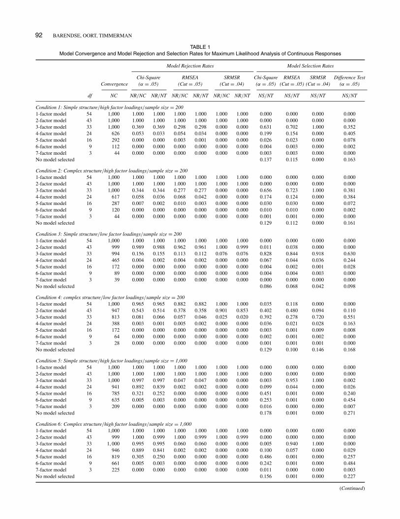
Table 1 gives rejection and selection rates for factor modelswith one through seven dimensions, for each of the eight con-ditions. The NC column shows the number of data sets withwhich the ML method converged to a solution. We note thatconvergence is almost always achieved with one-, two-, andthree-factor models, but that convergence becomes very dif-ficult with models with more factors, especially when samplesizes are small (as in Conditions 1–4).
Next, Table 1 gives the rejection rates according to sig-nificant chi-square values (α = .05), RMSEA values largerthan .05, and SRMSR values larger than .04. These rejec-tion rates are calculated both as proportions of successfulanalyses (NR/NC) and as proportions of the total numberof analyses (NR/NT). The two proportions do not differmuch, once more indicating that nonconvergence is causedby trying to fit models with redundant factors.
As an aside, we note that the rejection rates accordingto chi-square and RMSEA values are close to the expectedrejection rates that can be calculated on the basis of thenoncentral chi-square distribution, but only for the three-factor model, and only after correcting the fit results by(N – 1)/N (as Mplus uses N as the multiplier of the dis-crepancy function). Models with fewer factors do not meetthe regularity assumptions for calculating the noncentralityparameter (Steiger, Shapiro, & Browne, 1985). For mod-els with more than three factors, the rejection rates arebiased because of frequent convergence problems. It shouldbe noted that the estimation of the noncentrality parame-ter could be problematic anyway (Olsson, Foss, & Breivik,2004).
Finally, Table 1 gives the selection rates for each model,according to the procedure of selecting the first model thatfits, using the chi-square, RMSEA, and SRMSR fit cri-teria, and the procedure of selecting the last model thatsignificantly improves fit, using the chi-square differencetest (α = .05). As expected, the procedures that use thechi-square test generally select models with larger num-bers of factors than procedures that use the RMSEA index.In addition, models with larger numbers of factors are morefrequently selected in conditions with large sample size,high factor loadings, and simple structure than in conditionswith small sample size, low factor loadings, and complexstructure.
Of course, rejection and selection rates primarily dependon the arbitrary choices of a level of significance for the chi-square test and cutoffs for the RMSEA and SRMSR indices.
Discrete Responses
Discrete data have been analyzed with five estimation meth-ods: ML of covariances, ML of polychoric correlations,MLR, WLS, and WLSMV. Full results can be downloadedfrom the website of the corresponding author.1 Here we sum-marize the results in two ways. First, we consider rejectionand selection rates across all conditions with discrete data(in Tables 2 and 3, to be discussed later). Second, we exam-ine differences in model selection between conditions andestimation methods, using ordinal logistic regression anal-yses (Tables 4 and 5). When summarizing the results, weonly consider the results of ML of covariances, WLS, andWLSMV. We refrain from further presenting the results ofMLR and ML of polychoric correlations, because they showproblematic behavior in this study. With MLR estimation,the rejection rates are consistently above zero, even for mod-els with large numbers of factors, due to an inconsistentestimate of the MLR scaling correction factor. This inconsis-tency also causes frequent negative chi-square differences.Furthermore, MLR estimation is associated with the high-est proportions of nonconvergence of all estimation methods(Table 6). Moreover, the selection procedure that relies onthe chi-square difference test often fails to select any model(e.g., in 34% of the small sample cases and in 48% of thelarge sample cases) with MLR. With ML of polychoric corre-lations, the rejection rates are unreasonably high. As a result,selection procedures that rely on the chi-square test fail toselect any model in the majority of small sample size cases(see footnote 1).
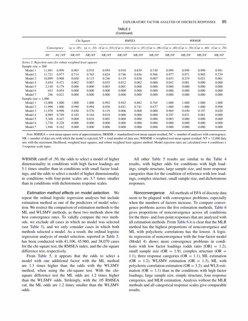
Rejection rates. Table 2 gives the rejection rates forML, WLS, and WLSMV analyses with various fit crite-ria, for small sample conditions and large sample con-ditions separately, but across all other conditions, andacross dichotomous, three-point, and four-point responsescales, totaling 12,000 data sets for each estimation method.Numbers and proportions of data sets with which conver-gence was successful are given in the NC and NC/NTcolumns.
With ML analysis of covariances, the convergencepercentages for the four-factor model are just 41.2% in smallsample conditions and 72.2% in large sample conditions,and even worse for models with more factors. It appears thatwith the common .05 cutoff choice for the RMSEA, Model3 is rejected in 8.3% of the small sample cases and in only0.1% of the large sample cases, whereas the chi-square testis significant at the 5% level in 0.1% and 55.0% of the smalland large sample cases, respectively. In contrast with thechi-square tests that gain power with larger sample sizes,
1Tables with full results of all estimation methods and fit crite-ria can be downloaded from the website of the corresponding authorat http://www.uva.nl/over-de-uva/organisatie/medewerkers/content/o/o/f.j.oort/f.j.oort.html or http://tinyurl.com/d7e7c64 (under Miscellaneous:Exploratory Factor Analysis of Discrete Data).
Note. RMSEA = root mean square error of approximation; SRMSR = standardized root mean square residual; NC = number of analyses with convergence;NR = number of data sets with which the model is rejected; NT = total number of data sets (1,000); NS = number of data sets with which the model is selected.
both RMSEA and SRMSR results show smaller rejectionrates with larger sample sizes. Even with an SRMSR cutoffas small as .03, Model 3 is never rejected in large samplecases.
The rejection rates with WLS estimation generally showthe same picture as those with ML estimation, but with WLSestimation the convergence percentages are lower: 33.0%and 66.7% for the four-factor model in small and largesample conditions.
The WLSMV estimation method has better convergencethan the ML and WLS estimation methods: 47.1% and74.9% percent for the four-factor model in small and largesample conditions. In small sample conditions, the three-factor model is rejected in 5.8% of the cases by the chi-square test at α = .05 and in 3.8% of the cases by RMSEAcutoff at .05. In large sample conditions, the chi-square testhas more power and rejects the three-factor model in 45.8%of the cases. Yet the three-factor model is never rejected bythe .05 RMSEA cutoff in large sample conditions. With theWRMSR index, with a .50 cutoff, Model 3 is rejected in21.9% of the small sample cases and in 65.0% of the largesample cases.
Selection rates. Table 3 gives the model selection ratesfor ML, WLS, and WLS estimation with various fit criteria.In the small sample size conditions, both the chi-square testand the RMSEA index select Model 3 most of the time. In thelarge sample conditions, the RMSEA index selects Model3 even more frequently than in the small sample conditions,
whereas the chi-square test more frequently points to modelswith larger numbers of factors. As expected, the chi-squaredifference test generally selects models with more factorsthan the stand-alone chi-square test, but it also more oftenends up without selecting a model.
Convergence problems hinder model selection, especiallyin small sample conditions, and especially with the WLSestimation procedure, as it fails to select a model in 30.9%of the cases with the chi-square test (α = .05), in 35.5% ofthe cases with the chi-square difference test (α = .05), andin 26.8% of the cases with the RMSEA (cutoff = .05).
The WLS estimation procedure shows the lowest percent-ages of selection failures. With WLS, the chi-square test atα = .05, the .05 RMSEA cutoff, the .50 WRMSR cutoff, andthe chi-square difference test at α = .05, all select Model 3 inmore than 60% of the small sample cases. In the large samplecases, the .50 WRMSR cutoff and the chi-square tests morefrequently select models with higher numbers of factors.
Condition effects on model selection. To summa-rize the effects of different conditions and response scaleson model selection, Table 4 gives the results of ordinallogistic regression analyses for each estimation method (MLof covariances, WLS, WLSMV) and five fit criteria (chi-square test with α = .05, RMSEA index with cutoff .05,SRMSR index with cutoff .04, WRMSR index with cutoff.50, chi-square difference test with α = .05), with the num-ber of factors as the dependent variable, and the manipulatedfactors as predictors (using dummy coding).
94 BARENDSE, OORT, TIMMERMAN
The first part of Table 4 shows the effects on modelselection through ML estimation. It appears that with thechi-square test, the odds to select a model of higherdimensionality in conditions with high factor loadings are12.3 times higher than in conditions with small factor load-ings. Likewise, the odds to select a model with an additionalfactor in conditions with simple structure are 1.8 times higherthan in conditions with complex structure, and the odds inlarge sample size conditions are 42.3 times higher than insmall sample size conditions. The odds to select a modelwith an additional factor in conditions with three-point, four-point, and continuous responses are 3.2, 4.9, and 16.0 timeshigher than in conditions with dichotomous responses.
The other fit criteria show a similar picture, with theexception of the sample size effect on model selection withthe SRMSR. With the SRMSR, the odds to select modelswith more factors are smaller in large sample conditions than
in small sample conditions (i.e., 29.0 times smaller). We fur-ther note that the simple structure effect on model selectionis much higher with the RMSEA and SRMSR indices thanwith the chi-square tests.
With WLS and WLSMV estimation, we generally see thesame pattern in most selection procedures: The odds to selectmodels with larger numbers of factors are higher with highfactor loadings, simple structure, large sample size, and moreresponse categories. With WLS, the sample size effect onmodel selection with RMSEA is an exception, as the oddsto select models with more factors are 5.6 times smallerin large sample conditions than in small sample conditions.This might be due to the convergence problems with smallsample sizes.
In the selection procedure through WLSMV estimation,the WRMSR index is new and behaves contrary to theSRMSR index in the ML procedure. For example, with the
TABLE 2Rejection Rates According Different Estimation Methods, Various Fit Criteria and Cutoff Values, Across All Conditions With Discrete Responses
Note. RMSEA = root mean square error of approximation; SRMSR = standardized root mean square residual; NC = number of analyses with convergence;NR = number of data sets with which the model is rejected; NT = total number of data sets; WRMSR = weighted root mean square residual. NT = 12,000 datasets with the maximum likelihood, weighted least squares, and robust weighted least squares method. Model rejection rates are calculated over 4 conditions x3 response scale types.
WRMSR cutoff of .50, the odds to select a model of higherdimensionality in conditions with high factor loadings are5.1 times smaller than in conditions with small factor load-ings, and the odds to select a model of higher dimensionalityin conditions with four-point scales are 3.7 times smallerthan in conditions with dichotomous response scales.
Estimation method effects on model selection. Werepeat the ordinal logistic regression analyses but includeestimation method as one of the predictors of model selec-tion. We restrict the comparison of estimation methods to theML and WLSMV methods, as these two methods show thebest convergence rates. To validly compare the two meth-ods, we exclude all cases in which no model was selected(see Table 3), and we only consider cases in which bothmethods selected a model. As a result, the ordinal logisticregression analysis of model selection, reported in Table 5,has been conducted with 41,106, 45,960, and 38,070 casesfor the chi-square test, the RMSEA index, and the chi-squaredifference test, respectively.
From Table 5, it appears that the odds to select amodel with one additional factor with the ML methodare 1.3 times higher than the odds with the WLSMVmethod, when using the chi-square test. With the chi-square difference test the ML odds are 1.2 times higherthan the WLSMV odds. Strikingly, with the .05 RMSEAcut, the ML odds are 1.2 times smaller than the WLSMVodds.
All other Table 5 results are similar to the Table 4results, with higher odds for conditions with high load-ings, simple structure, large sample size, and more responsecategories than for the condition of reference with low load-ings, complex structure, small sample size, and dichotomousresponses.
Nonconvergence. All methods of EFA of discrete dataseem to be plagued with convergence problems, especiallywhen the numbers of factors increase. To compare conver-gence problems across the five estimation methods, Table 6gives proportions of nonconvergence across all conditionsfor the three- and four-point responses that are analyzed withall estimation methods. From Table 6 it is clear that the MLRmethod has the highest proportions of nonconvergence andML with polychoric correlations has the lowest. A logis-tic regression of nonconvergence with the four-factor model(Model 4) shows more convergence problems in condi-tions with low factor loadings (odds ratio [OR] = 1.2),small sample size (OR = 1.9), complex structure (OR =1.1), three response categories (OR = 1.1), ML estimation(OR = 1.2), WLSMV estimation (OR = 1.3), ML withpolychoric correlation estimation (OR = 3.2), and WLS esti-mation (OR = 1.1) than in the conditions with high factorloadings, large sample size, simple structure, four responsecategories, and MLR estimation. Analysis without the MLRmethods and all categorical response scales give comparableresults.
TAB
LE3
Sel
ectio
nR
ates
Acc
ordi
ngto
Diff
eren
tEst
imat
ion
Met
hods
,Var
ious
Fit
Crit
eria
and
Cut
offV
alue
s,A
cros
sA
llC
ondi
tions
With
Dis
cret
eR
espo
nses
Chi
-Squ
are
RM
SEA
SRM
SRD
iffer
ence
Test
(α=
.05)
(α=
.10)
(Cut
=.0
3)(C
ut=
.04)
(Cut
=.0
5)(C
ut=
.06)
(Cut
=.0
2)(C
ut=
.03)
(Cut
=.0
4)(C
ut=
.05)
(α=
.05)
(α=
.10)
NS/
NT
NS/
NT
NS/
NT
NS/
NT
NS/
NT
NS/
NT
NS/
NT
NS/
NT
NS/
NT
NS/
NT
NS/
NT
NS/
NT
Seri
es1:
Sele
ctio
nra
tes
for
max
imum
like
liho
odSa
mpl
esi
ze=
200
Mod
el1
0.08
70.
017
0.03
60.
083
0.15
30.
252
0.00
00.
000
0.00
00.
017
0.00
00.
000
Mod
el2
0.17
70.
282
0.11
20.
152
0.18
30.
199
0.00
00.
000
0.04
20.
282
0.10
10.
091
Mod
el3
0.56
00.
644
0.44
60.
513
0.53
90.
505
0.00
40.
389
0.80
10.
644
0.53
00.
493
Mod
el4
0.05
60.
007
0.10
90.
072
0.04
10.
013
0.13
60.
210
0.02
70.
007
0.19
30.
186
Mod
el5
0.00
90.
003
0.02
40.
015
0.00
60.
002
0.11
10.
031
0.00
70.
003
0.01
60.
016
Mod
el6
0.00
30.
001
0.00
80.
005
0.00
20.
001
0.03
00.
011
0.00
30.
001
0.00
10.
001
Mod
el7
0.00
20.
000
0.00
60.
003
0.00
10.
000
0.01
30.
006
0.00
10.
000
0.00
00.
000
No
mod
el0.
106
0.04
60.
259
0.15
80.
075
0.02
90.
707
0.35
30.
118
0.04
60.
159
0.21
3Sa
mpl
esi
ze=
1,00
0M
odel
10.
000
0.00
00.
007
0.05
90.
155
0.26
40.
000
0.00
40.
125
0.25
10.
000
0.00
0M
odel
20.
010
0.00
60.
057
0.12
30.
148
0.10
80.
001
0.15
20.
183
0.25
10.
014
0.01
3M
odel
30.
436
0.34
30.
728
0.79
70.
697
0.62
70.
902
0.84
40.
692
0.49
80.
236
0.20
6M
odel
40.
286
0.28
70.
130
0.01
70.
000
0.00
00.
068
0.00
00.
000
0.00
00.
339
0.30
7M
odel
50.
095
0.12
30.
027
0.00
20.
000
0.00
00.
005
0.00
00.
000
0.00
00.
176
0.17
0M
odel
60.
022
0.03
10.
006
0.00
00.
000
0.00
00.
002
0.00
00.
000
0.00
00.
033
0.03
2M
odel
70.
009
0.01
30.
003
0.00
00.
000
0.00
00.
001
0.00
00.
000
0.00
00.
000
0.00
0N
om
odel
0.14
20.
197
0.04
20.
002
0.00
00.
000
0.02
10.
000
0.00
00.
000
0.20
20.
272
Seri
es2:
Sele
ctio
nra
tes
for
wei
ghte
dle
asts
quar
esSa
mpl
esi
ze=
200
Mod
el1
0.01
00.
005
0.00
30.
008
0.02
30.
062
––
––
0.00
00.
000
Mod
el2
0.11
30.
078
0.04
70.
087
0.16
20.
260
––
––
0.04
10.
030
Mod
el3
0.47
70.
420
0.31
20.
407
0.47
40.
472
––
––
0.38
50.
336
Mod
el4
0.07
80.
102
0.12
30.
097
0.06
10.
030
––
––
0.20
70.
198
Mod
el5
0.01
10.
014
0.02
30.
015
0.00
90.
004
––
––
0.01
20.
012
Mod
el6
0.00
20.
003
0.00
50.
003
0.00
10.
001
––
––
0.00
00.
000
Mod
el7
0.00
20.
002
0.00
30.
002
0.00
10.
000
––
––
0.00
00.
000
No
mod
el0.
309
0.37
50.
484
0.38
10.
268
0.17
1–
––
–0.
355
0.42
4Sa
mpl
esi
ze=
1,00
0M
odel
10.
000
0.00
00.
010
0.07
70.
198
0.30
6–
––
–0.
000
0.00
0M
odel
20.
014
0.00
80.
072
0.15
20.
191
0.27
2–
––
–0.
001
0.00
0M
odel
30.
466
0.36
40.
759
0.76
00.
611
0.42
2–
––
–0.
248
0.21
1M
odel
40.
254
0.26
60.
093
0.00
80.
000
0.00
0–
––
–0.
361
0.33
1M
odel
50.
068
0.09
50.
016
0.00
10.
000
0.00
0–
––
–0.
149
0.14
4M
odel
60.
015
0.02
10.
004
0.00
00.
000
0.00
0–
––
–0.
022
0.02
2M
odel
70.
006
0.01
00.
001
0.00
00.
000
0.00
0–
––
–0.
000
0.00
0N
om
odel
0.17
70.
236
0.04
50.
003
0.00
00.
000
––
––
0.21
90.
292
(Con
tinu
ed)
96
TAB
LE3
(Con
tinue
d)
Chi
-Squ
are
RM
SEA
WR
MSR
Diff
eren
ceTe
st
(α=
.05)
(α=
.10)
(Cut
=.0
3)(C
ut=
.04)
(Cut
=.0
5)(C
ut=
.06)
(Cut
=.4
0)(C
ut=
.50)
(Cut
=.6
0)(C
ut=
.70)
(α=
.05)
(α=
.10)
NS/
NT
NS/
NT
NS/
NT
NS/
NT
NS/
NT
NS/
NT
NS/
NT
NS/
NT
NS/
NT
NS/
NT
NS/
NT
NS/
NT
Seri
es3:
Sele
ctio
nra
tes
for
robu
stw
eigh
ted
leas
tsqu
ares
Sam
ple
size
=20
0M
odel
10.
097
0.06
50.
040
0.08
90.
160
0.25
00.
000
0.00
00.
000
0.00
90.
000
0.00
0M
odel
20.
176
0.15
40.
118
0.15
10.
175
0.18
00.
000
0.00
60.
071
0.23
10.
111
0.10
4M
odel
30.
644
0.63
30.
550
0.61
30.
610
0.55
50.
255
0.68
40.
832
0.71
90.
638
0.61
2M
odel
40.
034
0.06
00.
103
0.05
60.
022
0.00
60.
282
0.10
90.
018
0.00
60.
154
0.15
2M
odel
50.
004
0.00
80.
020
0.00
90.
003
0.00
10.
043
0.01
30.
004
0.00
10.
008
0.00
8M
odel
60.
001
0.00
20.
004
0.00
20.
001
0.00
00.
009
0.00
30.
001
0.00
00.
000
0.00
0M
odel
70.
000
0.00
10.
002
0.00
10.
000
0.00
00.
003
0.00
10.
000
0.00
00.
000
0.00
0N
om
odel
0.04
40.
077
0.16
30.
079
0.02
80.
009
0.40
80.
184
0.07
30.
034
0.08
90.
124
Sam
ple
size
=1,
000
Mod
el1
0.00
00.
000
0.00
80.
057
0.13
80.
236
0.00
00.
000
0.00
00.
000
0.00
00.
000
Mod
el2
0.01
00.
006
0.05
40.
103
0.12
10.
088
0.00
00.
000
0.00
00.
002
0.00
10.
001
Mod
el3
0.53
10.
417
0.81
90.
835
0.74
10.
677
0.02
90.
348
0.80
10.
976
0.28
70.
253
Mod
el4
0.26
90.
294
0.08
40.
005
0.00
00.
000
0.42
90.
447
0.14
00.
015
0.37
90.
353
Mod
el5
0.07
60.
107
0.01
50.
000
0.00
00.
000
0.18
10.
043
0.01
10.
001
0.17
20.
168
Mod
el6
0.01
60.
025
0.00
30.
000
0.00
00.
000
0.03
30.
012
0.00
40.
000
0.03
00.
029
Mod
el7
0.00
70.
012
0.00
20.
000
0.00
00.
000
0.02
30.
008
0.00
20.
000
0.00
00.
000
No
mod
el0.
091
0.13
80.
016
0.00
00.
000
0.00
00.
304
0.14
20.
043
0.00
60.
131
0.19
7
Not
e.R
MSE
A=
root
mea
nsq
uare
erro
rof
appr
oxim
atio
n;SR
MSR
=st
anda
rdiz
edro
otm
ean
squa
rere
sidu
al;N
S=
num
ber
ofda
tase
tsw
ithw
hich
the
mod
elis
sele
cted
;NT
=to
taln
umbe
rof
data
sets
;WR
MSR
=w
eigh
ted
root
mea
nsq
uare
resi
dual
.NT
cont
ains
12,0
00da
tase
tsw
ithth
em
axim
umlik
elih
ood,
wei
ghte
dle
asts
quar
es,a
ndro
bust
wei
ghte
dle
asts
quar
esm
etho
d.M
odel
sele
ctio
nra
tes
are
calc
ulat
edov
er4
cond
ition
s×
3re
spon
sesc
ale
type
s.
97
98 BARENDSE, OORT, TIMMERMAN
TABLE 4Ordinal Logistic Regression Analysis of Model Selection, for Different Estimation Methods According to Various Fit Criteria, Across All
Note. RMSEA = root mean square error of approximation; SRMSR = standardized root mean square residual; OR = odds ratio; WRMSR = weightedroot mean square residual. The condition of reference has small factor loadinfs, complex structure, small sample size,and dichotmous response scales. Withmaximum likerlihood estimation, the regression analysis is based on 32,000 data sets and with weighted least squares and robust weighted least squares on24,000 data sets.
TABLE 5Ordinal Logistic Regression of Model Selection With the Maximum Likelihood and Robust Weighted Least Squares Methods, Across All
Conditions With Dichotomous, Three-Point, and Four-Point Response Scales
Note. RMSEA = root mean square error od approximation; OR = odds ratio. β is the log odds ratio and OR is the ratio of odds of model selection inthe particular condition over the odds in the condition of reference. The condition of reference is small loadings, complex structure, small sample size, anddichotomous response scales, analyzed with the weighted least squares method. For chi-square tests, odds ratios are calculated for 41,106 data sets: 13,796,13,682, and 13,628 cases with dichotomous, three-point, and four-point responses, respectively. For RMSEA indices, odds ratios are calculated for 45,960 datasets: 15,290, 15,342, and 15,328 cases with dichotomous, three-point, and four-point responses, respectively. For chi-square difference tests, odds ratios arecalculated for 38,070 data sets: 12,550, 12,810, and 12,710 cases with dichotomous, three-point, and four-point responses, respectively.
DISCUSSION
We compared different estimation methods, with differentfit criteria, under various conditions, but judgment of pre-ferred methods and criteria depends on the goals of the
user. We used a model with three major factors and fourminor factors to generate data with six dimensions (six,not seven, because of our parameterization choices). If theresearcher would like to recover six factors, he or she mightprefer the chi-square test that is a measure of exact fit.
EXPLORATORY FACTOR ANALYSIS OF DISCRETE RESPONSES 99
TABLE 6Proportions of Nonconvergence, Calculated Across All Conditions
Note. ML = maximum likelihood; MLR = robust maximum likelihood;WLSMV = robust weighted least squares; WLS = weighted least squares.The total number of data sets in these conditions is 16,000.
The chi-square test and chi-square difference test proce-dures generally select models with more common factorsthan the RMSEA and the SRMSR or WRMSR procedures,but hardly ever the six-factor model. This is consistent withthe study of Briggs and MacCallum (2003) with continu-ous data that showed difficulties recovering patterns withminor factors that were even larger than ours. In con-trast, simulation studies of models with only major factorsencountered overextraction problems (e.g., Beauducel, 2001;Hayashi et al., 2007). The chi-square difference test proce-dure recovers more factors than the stand-alone chi-squaretest procedure, but it also more frequently ends up withoutselecting any model, because of nonconvergence problems.
If the researcher is primarily interested in major factors,he or she might want to rely on the RMSEA index. Forexample, with the robust WLS estimation method, and withthe common choice of a .05 cutoff, the RMSEA selectsthe three-factor model in 61.0% of the small sample casesand in 74.1% of the large sample cases. For the chi-squaretest procedure, these selection percentages are 64.4% and53.1%. Interestingly, the WRMSR with .60 and .70 cut-offs outperformed the RMSEA procedure in selecting thethree-factor model. Obviously, selection rates largely dependon the (arbitrary) choices of a level of significance for thechi-square tests and cutoffs for the RMSEA and RMSRindices. Marsh, Hau, and Wen (2004) and Hooper, Coughlan,and Mullen (2008) discussed model selection guidelines formodel selection in structural equation modeling of varianceand covariances of continuous data; less is known aboutdiscrete data.
Selection rates also depend on circumstances. Chi-squaretests and RMSEA index procedures recover more factorswhen sample size is larger, when factor loadings are higher,when factor structure is less complex, and when the responsescales have more options. The effects of sample size andcommunality (size of factor loadings) have also been foundin studies of factor pattern recovery (MacCallum, Widaman,Preacher, & Hong, 2001; MacCallum, Widaman, Zhang, &Hong, 1999). When model selection is based on the SRMSR
index, we find an opposite effect of sample size, as theSRMSR gets smaller with larger sample size, which can beexplained by the more precise correlation estimates on whichthe SRMSR is based. Conspicuously, all effects on modelselection with the WRMSR index are opposite to those ofthe SRMSR index.
For the purpose of clarity of presentation, we have onlyreported main effects of sample size, factor loading size, fac-tor structure complexity, and number of response options.However, for example, as apparent in Table 1, the effect ofthe factor loading size varies with sample size and factorstructure complexity. Full results of all estimation methodsand fit criteria can be downloaded from the website of thecorresponding author.
With all estimation methods, EFA is hindered by con-vergence problems, especially when the numbers of factorsincrease and when the sample size is small. To preventconvergence problems, we examined various rotation con-straints and we experimented with starting values. With theMplus computer program, the echelon form rotation con-straint appears to work best. Of all estimation methods thathave been used in our study, the WLSMV method is the pre-ferred method of choice. The ML methods lack theoreticaljustification for use with discrete data. The MLR methodhas the problem that the chi-square difference test oftenyields negative results, although we should note that Satorraand Bentler recently suggested a new procedure that consis-tently yields positive results (Asparouhov & Muthén, 2010;Satorra & Bentler, 2010). In our study, the ML estimationand WLSMV estimation do not show large differences inmodel selection, but Beauducel and Herzberg (2006) showedthat the WLSMV estimates are more precise with only a fewresponse options.
In conclusion, the WLSMV estimation method is theoret-ically justified for the factor analysis of discrete data and itgives the best results. In addition, this limited informationmethod of analyzing polychoric correlations is more prac-tical, as full information methods such as maximizing thelikelihood of observed response patterns are too computa-tionally intensive to be used in practice, even with smallnumbers of variables (Jöreskog & Moustaki, 2001; Wirth &Edwards, 2007).
FUNDING
This publication is supported by an open competitiongrant 400–09–084 from the Netherlands Organization forScientific Research (NWO).
REFERENCES
Asparouhov, T., & Muthén, B. (2010). Simple second order chi-squarecorrection. Mplus Technical Appendix. Retrieved from http://statmodel.com/download/WLSMV_new_chi21.pdf
Asparouhov, T., Muthén, M., & Muthén, B. (2006). Robust chi square dif-ference testing with mean and variance adjusted test statistics. Mplus WebNotes. Retrieved from http://www.statmodel.com/download/webnotes/webnote.pdf
Beauducel, A. (2001). On the generalizability of factors: The influence ofchanging contexts of variables on different methods of factor extraction.Methods of Psychological Research Online, 6, 1–28.
Beauducel, A., & Herzberg, P. (2006). On the performance of maximumlikelihood versus means and variance adjusted weighted least square esti-mation in confirmatory factor analysis. Structural Equation Modeling, 13,186–203.
Briggs, N. E., & MacCallum, R. C. (2003). Recovery of weak commonfactors by maximum likelihood and ordinary least squares estimation.Multivariate Behavioral Research, 38, 25–56.
Browne, M. W. (1982). Covariance structures. In Topics in appliedmultivariate analysis, ed. D. M. Hawkins (pp. 72–141). Cambridge, UK:Cambridge University Press.
Browne, M. W. (1984). Asymptotically distribution-free methods in theanalysis of covariance structures. British Journal of Mathematical andStatistical Psychology, 37, 62–83.
Browne, M. W., & Cudeck, R. (1992). Alternative ways of assessing modelfit. Sociological Methods and Research, 21, 230–258.
Conway, J. M., & Huffcutt, A. I. (2003). A review and evaluationof exploratory factor analysis practices in organizational research.Organizational Research Methods, 6, 147–168.
Dolan, C. V. (1994). Factor analysis of variables with 2, 3, 5 and 7 responsecategories: A comparison of categorical variable estimators using simu-lated data. British Journal of Mathematical and Statistical Psychology,47, 309–326.
Fabrigar, L. R., Wegener, D. T., MacCallum, R. C., & Strahan, E. J.(1999). Evaluating the use of exploratory factor analysis in psychologicalresearch. Psychological Methods, 4, 272–299.
Flora, D. B., & Curran, P.J. (2004). An empirical evaluation of alternativemethods of estimation for confirmatory factor analysis with ordinal data.Psychological Methods, 9, 466–491.
Hayashi, K., Bentler, P. M., & Yuan, K. H. (2007). On the likelihood ratiotest for the number of factors in exploratory factor analysis. StructuralEquation Modeling, 14, 505–526.
Holgado-Tello, F. P., Chacón-Moscoso, S., Barbero-García, I., & Vila-Abad,E. (2010). Polychoric versus Pearson correlations in exploratory andconfirmatory factor analysis of ordinal variables. Quality and Quantity,44, 153–166.
Hooper, D., Coughlan, J., & Mullen, M. R. (2008). Structural equationmodelling: Guidelines for determining model fit. Journal of BusinessResearch Methods, 6, 53–60.
Hu, L. T., & Bentler, P. M. (1999). Cutoff criteria for fit indexes in covari-ance structure analysis: Conventional criteria versus new alternatives.Structural Equation Modeling, 6, 1–55.
Johnson, D. R., & Creech, J. C. (1983). Ordinal measures in multipleindicator models: A simulation study of categorization error. AmericanSociological Review, 48, 398–407.
Jöreskog, K. G., & Moustaki, I. (2001). Factor analysis of ordinal variables:A comparison of three approaches. Mulitvariate Behavioral Research, 36,347–387.
Lord, F. M., & Novick, M. R. (1968). Statistical theories of mental testscores. Reading, MA: Addison-Wesley.
MacCallum, R. C., Browne, M. W., & Sugawara, H. M. (1996). Power anal-ysis and determination of sample size for covariance structure modeling.Psychological Methods, 1, 130–149.
MacCallum, R. C., Widaman, K. F., Preacher, K., & Hong, S. (2001).Sample size in factor analysis: The role of model error. MultivariateBehavioral Research, 36, 611–637.
MacCallum, R. C., Widaman, K. F., Zhang, S., & Hong, S. (1999). Samplesize in factor analysis. Psychological Methods, 4, 84–99.
Marsh, H. W., Hau, K. T., & Wen, Z. (2004). In search ofgolden rules: Comment on hypothesis testing approaches to set-ting cutoff values for fit indexes and dangers in overgeneralisingHu & Bentler’s (1999) findings. Structural Equation Modeling, 11,320–341.
Muthén, B. O. (1998–2004). Mplus technical appendices. Los Angeles,CA: Muthén & Muthén. Retrieved from http://statmodel.com/download/techappen.pdf
Muthén, B., du Toit, S. H., & Spisic, D. (1997). Robust inference usingweighted least squares and quadratic estimating equations in latent vari-able modeling with categorical and continuous outcomes. Psychometrika,75, 1–45.
Muthén, B., & Kaplan, D. (1985). A comparison of some methodologiesfor the factor analysis of non-normal Likert variables. British Journal ofMathematical and Statistical Psychology, 38, 171–189.
Muthén, B., & Kaplan, D. (1992). A comparison of some methodologies forthe factor analysis of non-normal Likert variables: A note on the size ofthe model. British Journal of Mathematical and Statistical Psychology,45, 19–30.
Muthén, B. O., & Muthén, L. K. (2010). Mplus user’s guide: Statisticalanalysis with latent variables. Los Angeles, CA: Muthén & Muthén.
Olsson, U. H., Foss, T., & Breivik, E. (2004). Two equivalent dis-crepancy functions for maximum likelihood estimation: Do theirtest statistics follow a non-central chi-square distribution undermodel misspecification? Sociological Methods Research, 32,453–500.
Olsson, U. H., Troye, S. V., & Howell, R. D. (1999). Theoretic fit andempirical fit: The performance of maximum likelihood versus generalizedleast squares estimation in structural equation modeling. MultivariateBehavioral Research, 34, 31–58.
Preacher, K. J., & MacCallum, R. C. (2003). Repairing Tom Swift’s electricfactor analysis machine. Understanding Statistics, 2, 13–32.
Rhemtulla, M., Brosseau-Liard, P., & Savalei, V. (2012). When can categori-cal variables be treated as continuous? A comparison of robust continuousand categorical SEM estimation methods under suboptimal conditions.Psychological Methods, 17(3), 354.
Rigdon, E. E., & Ferguson, C. E. (1991). The performance of the polychoriccorrelation coefficient and selected fitting functions in confirmatory fac-tor analysis with discrete data. Journal of Marketing Research, 28,491–497.
Satorra, A., & Bentler, P. M. (1994). Corrections to test statistics and stan-dard errors in covariance structure analysis. In A. von Eye & C. C.Clogg (Eds.), Latent variables analysis: Applications for developmentalresearch (pp. 399–419). Thousand Oaks, CA: Sage.
Satorra, A., & Bentler, P. M. (2001). A scaled difference chi-square teststatistic for moment structure analysis. Psychometrika, 66, 507–514.
Satorra, A., & Bentler, P. M. (2010). Ensuring positiveness of the scaleddifference chi-square test statistic. Psychometrika, 75, 243–248.
Sivo, S. A., Fan, X., Witta, E. L., & Willse, J. T. (2006). The search for “opti-mal” cut-off properties: Fit index criteria in structural equation modeling.Journal of Experimental Education, 74, 267–288.
Steiger, J. H., Shapiro, A., & Browne, M. W. (1985). On the multivariateasymptotic distribution of sequential chi-square statistics. Psychometrika,50, 253–264.
Ten Holt, J. C., van Duijn, M. A. J., & Boomsma, A. (2010). Scale con-struction and evaluation in practice: A review of factor analysis versusitem response theory. Psychological Test and Assessment Modeling, 52,272–297.
Wirth, R. J., & Edwards, M. C. (2007). Item factor analysis: Currentapproaches and future directions. Psychological Methods, 12,58–79.
Yang-Wallentin, F., Jöreskog, K. G., & Luo, H. (2010). Confirmatory fac-tor analysis of ordinal variables with misspecified models. StructuralEquation Modeling, 17, 392–423.
EXPLORATORY FACTOR ANALYSIS OF DISCRETE RESPONSES 101
Yu, C. Y., & Muthén, B. (2002). Evaluation of model fit indices for latentvariable models with categorical and continuous outcomes (Technicalreport). Los Angeles, CA: University of California at Los Angeles,Graduate School of Education & Information Studies.
Yuan, K. H., & Bentler, P. M. (1998). Normal theory based test statisticsin structural equation modelling. British Journal of Mathematical andStatistical Psychology, 51, 289–309.
Yuan, K. H., & Bentler, P. M. (2000). Three likelihood-based methods formean and covariance structure analysis with nonnormal missing data. InM. E. Sobel & M. P. Becker (Eds.), Sociological methodology 2000 (pp.165–200). Washington, DC: ASA.
Zhang, J., & Stout, W. F. (1999). Conditional covariance structure ofgeneralized compensatory multidimensional items. Psychometrika, 64,129–152.