M39 KNIG2461 04 ISM C39 - media.physicsisbeautiful.com

© Copyright 2017 Pearson Education, Inc. All rights reserved. This material is protected under all copyright laws as they currently exist. No portion of this material may be reproduced, in any form or by any means, without permission in writing from the publisher.

39-1

Conceptual Questions

39.1. (a) At 1x ≈ because the probability density is higher there. (b) From Equation 39.14 we see that Prob(in at ) ( ) .x x P x xδ δ= If 1,000,000 photons are detected then the number

expected in a 1-mm-wide interval is 1,000,000 ( )P x xδ where 1.0 mm.xδ = For 10.50 m ( ) 1 mx P x −= = and the

number expected is 1(1,000,000)(1 m )(0.001 m) 1,000.− =

39.2. The relationship between probability and probability density is similar to the relationship between mass m and mass density .ρ Regions of higher mass density tell us where mass is concentrated. The mass itself is a more tangible quantity that depends both on the mass density and on the size of a specific piece of material. Similarly, probability density tells us regions in which a particle is more likely, or less likely, to be found. The probability is a definite number between 0 and 1. Probability depends both on the probability density and on the size of the specific region we are considering.

39.3. The probability of finding a particle at position x is determined by 2( ) ,xψ which is shown below.

The electron is most likely to be found at the point or points where 2( )xψ is a maximum. The graph given in the

problem shows ( ).xψ The figure above shows 2( ) .xψ Notice that 2 2( 0 nm) ( 2 nm) ,x xψ ψ= > = ± even though ( 0 nm) 0xψ = < in the original graph. Thus, the electron is most likely to be found at x = 0 nm. The electron is least

likely to be found where 2( )xψ is a minimum. From the figure, 2( ) 0 at 1 nm.x xψ = = ± Thus, the electron is least likely to be found at 1 nm.x = ±

39.4. (a) The probability density is maximum at 2 mmx = ± because the number of dots per unit length is greatest at these points. (b) We cannot tell where the wave function is most positive because the probability density is given by the absolute square of the wave function, so we lose the sign information. The most positive part of the wave function could be at either 2 mmx = or 2 mm,x = − or it could be most positive at 2 mm and most negative at the 2 mm− (or vice versa), or it could be most negative at both positions.

WAVE FUNCTIONS AND UNCERTAINTY

39

39-2 Chapter 39


39.5. The area under the probability density curve must be one. That is, ( )d 1.P x x∞

−∞

=∫ For this condition to be true

for Figure Q39.5, a must be 12 mm ,− because the area of a triangle is half the base times the height.

39.6. The particle with the most precisely known velocity has the smallest velocity uncertainty Δv. Because the three particles have equal masses, it also has the smallest momentum uncertainty Δp. From the uncertainty principle

/2,x p hΔ Δ ≥ the particle with the smallest momentum uncertainty must have the largest position uncertainty Δx. That is seen to be particle 1, whose wave function has the largest spatial extent. The wave function amplitude difference of particles 2 and 3 is not relevant; they both have Δx smaller than particle 1 and thus have a larger momentum and velocity uncertainty.

Exercises and Problems

Exercises Section 39.1 Waves, Particles, and the Double-Slit Experiment 39.1. Model: The sum of the probabilities of all possible outcomes must equal 1 (100%). Solve: The sum of the probabilities is A B C D 1. Hence,P P P P+ + + =

C D C D0 40 0 30 1 0 30P P P P. + . + + = ⇒ + = .

Because C D D D2 , 2 0.30.P P P P= + = This means D C0.10 and 0.20.P P= = Thus, the probabilities of outcomes C and D are 20% and 10%, respectively.

39.2. Model: The probability that the outcome will be A or B is the sum of A Band .P P Solve: (a)

Coin A Coin B Coin C H H H H H T H T H H T T T H H T H T T T H T T T

(b) From the above table, we see that 2 heads and 1 tail occur three times (HHT, HTH, THH). Out of the possible eight outcomes, each outcome is equally probable and has a probability of occurrence of 1/8. So, the probability of getting 2 heads and 1 tail is 3/8 = 37.5%. (c) From the table, we see that at least two heads occur 4 times (HHH, HHT, HTH, and THH). So, the probability of getting at least two heads is 4/8 = 50%.

39.3. Model: The probability that the outcome will be A or B is the sum of A Band .P P The expected value is your best possible prediction of the outcome of an experiment. Solve: For each deck, there are 12 picture cards (4 Jacks, 4 Queens, and 4 Kings). The probability of dealing one given card (say, a queen of hearts) out of 52 cards is 1/52, so the probability of dealing a picture card is 12(1/52) 23.1%.= Equation 39.5 tells us that the expected number of cards dealt is the probability multiplied by the number of trials,

expected face cardN NP=

The number of trials is 1000N = because we have 1000 decks and the probability of dealing a face card is face card 23.1%,P = so the number of face cards dealt is expected to be (1000)(0.231) = 231.

Wave Functions and Uncertainty 39-3


39.4. Model: The probability that the outcome will be A or B is the sum of A Band .P P Solve: (a) A regular deck of cards has 52 cards. Drawing a given card (say, queen of hearts) from this deck has a probability of 1/52. Because there are 4 aces in the deck, the probability of drawing an ace is 1/52 + 1/52 + 1/52 + 1/52 = 4(1/42) = 4/52 = 0.077 = 7.7%. (b) Because there are 13 spades, the probability of drawing a spade is 13(1/52) = 13/52 = 0.25 = 25%.

39.5. Model: The probability that the outcome will be A or B is the sum of A Band .P P Solve: (a) Each die has six faces and the faces are numbered from 1 to 6. We have two dice A and B. The various possible outcomes of rolling two dice are given in the following table.

A B A B A B 1 1 1 1 1 1 2 2 2 2 2 2

1 2 3 4 5 6 1 2 3 4 5 6

3 3 3 3 3 3 4 4 4 4 4 4

1 2 3 4 5 6 1 2 3 4 5 6

5 5 5 5 5 5 6 6 6 6 6 6

1 2 3 4 5 6 1 2 3 4 5 6

There are 36 possible outcomes. From the table, we find that there are six ways of rolling a 7 (1 and 6, 2 and 5, 3 and 4, 4 and 3, 5 and 2, 6 and 1). The probability is (1/36) × 6 = 1/6. (b) Likewise, the probability of rolling any double is 1/6. (c) There are 10 ways of rolling a 6 or an 8. The probability is (1/36) 10 5/18.× =

2 2

22 22

2000/N (10 V/m) (0 10 mm) (2000)(30 V/m) 18,000 / (30 V/m) (0 10 mm) (10 V/m)

NN N

.= ⇒ = =

.

Section 39.2 Connecting the Wave and Photon Views 39.6. Model: Combine Equations 39.10 and 39.11 to show that N is proportional to 2( ) .A x xδ

2 222 2 tot 2 2

2 1 1 1 11 1tot

(in at )( ) (in at )

(in at ) (in at )( )

N x xA x x N N x x

N x x N x xA x xN

δδ δ

δ δδ= =

We are given 1 1 1 26000, 0 10 mm, ( ) 200 V/m, 3000,N x A x Nδ= = . = = and 2 0 20 mm.xδ = . We are not given

totN but it cancels anyway.

Solve: Solve the above equation for 2( ) .A x

1 2 22 1

2 1 1

(in at ) (0 10 mm)(3000)( ) ( ) (200 V/m) 100 V/m(in at ) (0 20 mm)(6000)

x N x xA x A xx N x x

δ δδ δ

.= = =

.

Assess: The answer is half of the wave amplitude at the other strip, which seems reasonable.

39.7. Model: The probability density of finding a photon is directly proportional to the square of the light-wave amplitude 2( ) .A x Solve: The probability of finding a photon within a narrow region of width δ x at position x is

39-4 Chapter 39


212 1 1

22 2 2

( )Prob(in at )Prob(in at ) ( )Prob(in at ) ( )

A x xx xx x A x xx x A x x

δδδ δδ δ

∝ ⇒ =

Let N be the total number of photons and 2N the number of photons detected at 2x in a width δ x. The above equation simplifies to

2 2

22 22

2000/N (10 V/m) (0 10 mm) (2000)(30 V/m) 18,000 / (30 V/m) (0 10 mm) (10 V/m)

NN N

.= ⇒ = =

.

39.8. Solve: The probability that a photon arrives at this 0.10-mm-wide strip is

10Prob(in 0 10 mm at ) ( )1 0 10

Nx P x xδ. = =. ×

where N is the number of photons detected in the strip and the total number of photons is 101.0 10 .× We have

10 1 3 7(1 0 10 )(20 m )(0 10 10 m) 2 0 10N − −= . × . × = . ×

39.9. Model: See Example 39.1. Solve: We are given 12

tot 5 0 10 ,N = . × 9(in at ) 2 0 10 ,N x xδ = . × and 0 10 mmxδ = . . The probability that a photon

lands on the strip is 9 12Prob(in at ) 2 0 10 /5 0 10 0 00040.x xδ = . × . × = . Solve for the probability density ( )P x in Equation 39.12.

14

Prob(in at ) 0 00040( ) 4 0 m1 0 10 m

x xP xxδ

δ−

−.= = = .

. ×

Assess: This result is similar to the result of Example 39.1.

Section 39.3 The Wave Function 39.10. Solve: 2( )x xψ δ is a probability, which is dimensionless. The units of xδ are m, so the units of 2( )xψ

are 1m .− Thus the units of 1/2are m .ψ −

39.11. Visualize:



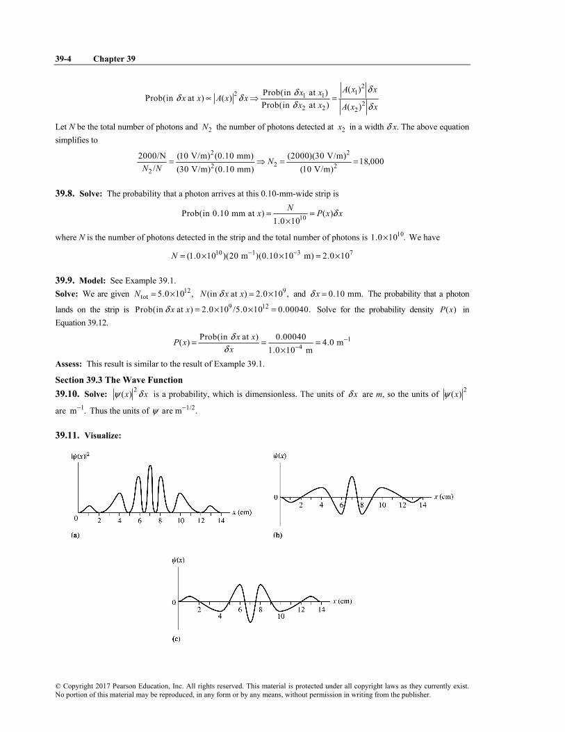
Solve: (a) We assume that 2( ) 0xψ = at some point in between each of the peaks. (b) Two factors are important for drawing ( ).xψ First, the value at each point is the square root of the value on the

2( )xψ graph. Second, and especially important, is that ( )xψ is a wave function and so it oscillates between positive

and negative values each time 2( )xψ reaches zero.

(c) Multiplying ( ) by 1xψ − does not change 2( ) .xψ So another possible graph for ( )xψ is the “upside down” version of the graph of part (b).

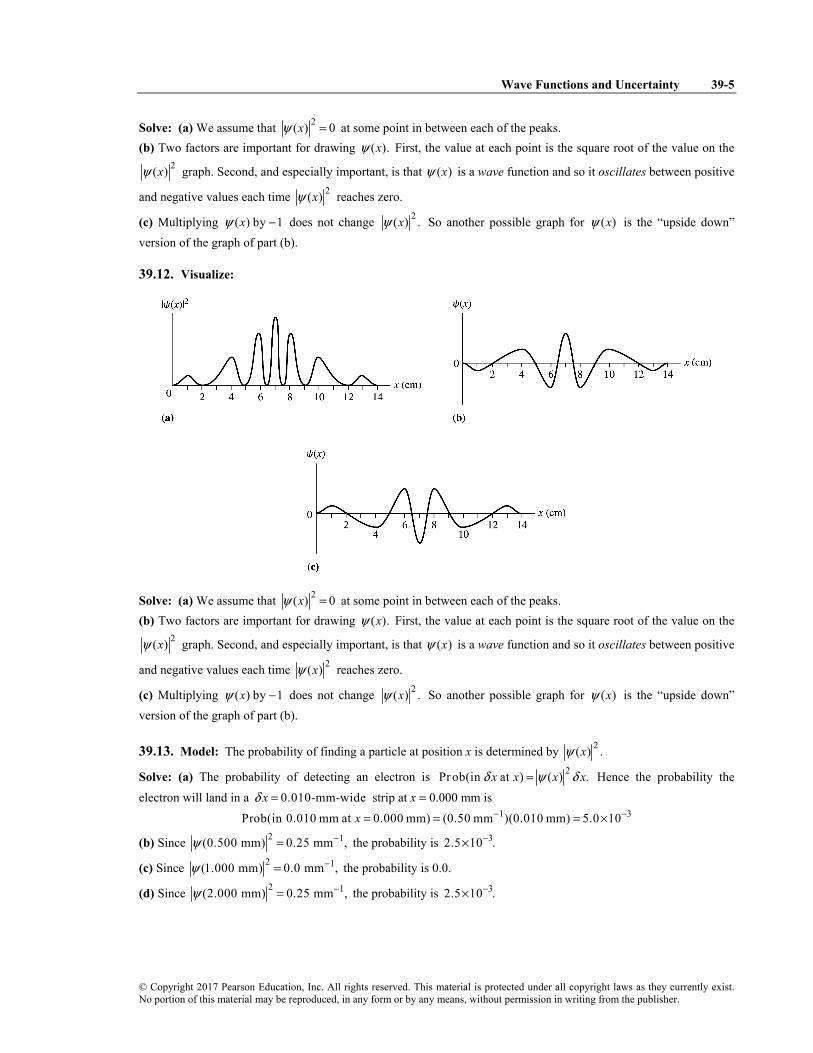
39.12. Visualize:

Solve: (a) We assume that 2( ) 0xψ = at some point in between each of the peaks. (b) Two factors are important for drawing ( ).xψ First, the value at each point is the square root of the value on the

2( )xψ graph. Second, and especially important, is that ( )xψ is a wave function and so it oscillates between positive

and negative values each time 2( )xψ reaches zero.

(c) Multiplying ( ) by 1xψ − does not change 2( ) .xψ So another possible graph for ( )xψ is the “upside down” version of the graph of part (b).

39.13. Model: The probability of finding a particle at position x is determined by 2( ) .xψ

Solve: (a) The probability of detecting an electron is 2Prob(in at ) ( ) .x x x xδ ψ δ= Hence the probability the electron will land in a 0.010-mm-widexδ = strip at x = 0.000 mm is

1 3Prob(in 0 010 mm at 0 000 mm) (0 50 mm )(0 010 mm) 5 0 10x − −. = . = . . = . ×

(b) Since 2 1(0 500 mm) 0 25 mm ,ψ −. = . the probability is 32.5 10 .−×

(c) Since 2 1(1 000 mm) 0 0 mm ,ψ −. = . the probability is 0.0.

(d) Since 2 1(2 000 mm) 0 25 mm ,ψ −. = . the probability is 32.5 10 .−×

39-6 Chapter 39


Section 39.4 Normalization 39.14. Model: The probability of finding a particle is determined by the probability density 2( ) ( ) .P x xψ=

Solve: (a) The normalization condition for a wave function: 2( ) area under the curve 1.x dxψ∞

−∞

= =∫ In the present

case, the area under the 2( )xψ -versus-x graph is 2 nm.a Hence, 112 nm .a −=

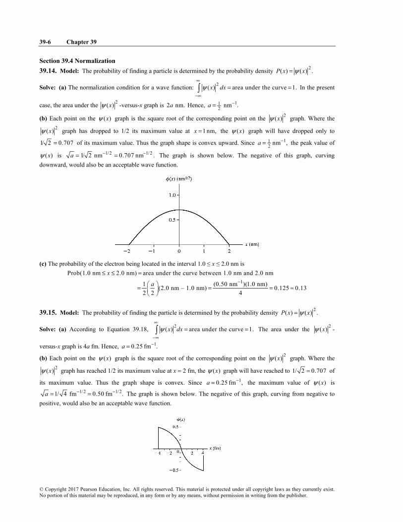
(b) Each point on the ( )xψ graph is the square root of the corresponding point on the 2( )xψ graph. Where the 2( )xψ graph has dropped to 1/2 its maximum value at 1 nm,x = the ( )xψ graph will have dropped only to

1/ 2 0.707= of its maximum value. Thus the graph shape is convex upward. Since 112 nm ,a −= the peak value of

( )xψ is 1/2 1/21/ 2 nm 0.707 nm .a − −= = The graph is shown below. The negative of this graph, curving downward, would also be an acceptable wave function.

(c) The probability of the electron being located in the interval 1.0 ≤ x ≤ 2.0 nm is

1

Prob(1.0 nm 2.0 nm) area under the curve between 1.0 nm and 2.0 nm

1 (0.50 nm )(1.0 nm)(2.0 nm – 1.0 nm) 0.125 0.132 2 4

x

a −

≤ ≤ =

⎛ ⎞= = = ≈⎜ ⎟⎝ ⎠

39.15. Model: The probability of finding the particle is determined by the probability density 2( ) ( ) .P x xψ=

Solve: (a) According to Equation 39.18, 2( ) area under the curve 1.x dxψ∞

−∞

= =∫ The area under the 2( )xψ -

versus-x graph is 4a fm. Hence, 10.25 fm .a −=

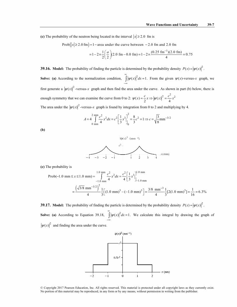
(b) Each point on the ( )xψ graph is the square root of the corresponding point on the 2( )xψ graph. Where the 2( )xψ graph has reached 1/2 its maximum value at x = 2 fm, the ( )xψ graph will have reached to 1/ 2 0.707= of

its maximum value. Thus the graph shape is convex. Since 10.25 fm ,a −= the maximum value of ( )xψ is 1/2 1/21/ 4 fm 0.50 fm .a − −= = The graph is shown below. The negative of this graph, curving from negative to

positive, would also be an acceptable wave function.



(c) The probability of the neutron being located in the interval 2.0x ≥ fm is

( )1

Prob 2.0 fm 1 area under the curve between 2 0 fm and 2 0 fm

1 (0 25 fm )(2 0 fm)1 2 (2 0 fm 0 0 fm) 1 2 0 752 2 4

x

a −

≥ = − − . .

. .⎛ ⎞= − × . − . = − × = .⎜ ⎟⎝ ⎠


Solve: (a) According to the normalization condition, 2( ) 1.x dxψ∞

−∞

=∫ From the given ( )-versus-x xψ graph, we

first generate a 2( ) -versus-x xψ graph and then find the area under the curve. As shown in part (b) below, there is

enough symmetry that we can examine the curve from 0 to 2: 2

2 2

2 4c cx x x xψ ψ( ) = ⇒ ( ) =

The area under the 2( ) -versus-x xψ graph is found by integration from 0 to 2 and multiplying by 4.

22 mm 22 2 3 2 3/2

0 mm 0

1 8 34 1 mm4 3 3 8cA x dx c x c c −⎡ ⎤= = = = ⇒ =⎢ ⎥⎣ ⎦∫

(b)

(c) The probability is

( )

1.0 mm1.0 mm 2 22 3

1.0 mm1.0 mm23/2 3

3 3 3

1Prob( 1.0 mm 1.0 mm)4 4 3

3/8 mm 1 3/8 mm 1 1(1.0 mm) ( 1.0 mm) [2(1.0 mm) ] 6.3%4 3 4 3 16

c cx x dx x−−

− −

⎡ ⎤− ≤ ≤ = = ⎢ ⎥⎣ ⎦

⎡ ⎤= − − = = =⎣ ⎦

∫


Solve: (a) According to Equation 39.18, 2( ) 1.x dxψ∞

−∞

=∫ We calculate this integral by drawing the graph of

2( )xψ and finding the area under the curve.

39-8 Chapter 39


The area of the 2( )xψ versus x graph is

1.0 nm 1.0 nm 2.0 nm2 2 2 2 2 2 2

2.0 nm 1.0 nm 1.0 nm2

1/2 1/2 1/2

( ) ( ) ( ) (0 25 )(1 0 nm) ( )(2 0 nm) (0 25 )(1 0 nm) 2 5

2 5 nm 1 01 0 nm 0.632 nm 0.63 nm2 5

x dx x dx x dx c c c c

c

c

ψ ψ ψ− −

− −

− − −

+ + = . . + . + . . = .

. = ..= = ≈.

∫ ∫ ∫

(b) The graph is shown in part (a). (c) The probability is

1.0 nm2 2 1

1.0 nm

1 0Prob( 1 0 nm 1 0 nm) ( ) ( )(2 0 nm) nm (2 0 nm) 0 802 5

x x dx cψ −

−

.⎛ ⎞− . ≤ ≤ . = = . = . = .⎜ ⎟.⎝ ⎠∫

Section 39.5 Wave Packets 39.18. Model: The beating of two waves of different frequencies produces a series of wave packets, or beats. Solve: The beat frequency is beat 1 2 502 Hz 498 Hz 4 Hz.f f f= − = − = The period of one beat is

beatbeat

1 1 0 25 s4 Hz

Tf

= = = .

During 0.25 s, the wave moves forward sound beat (340 m/s)(0.25 s) 85 m.x v TΔ = = = Thus the length of each wave packet is 85 m.

39.19. Model: A laser pulse is an electromagnetic wave packet, hence it must satisfy the relationship 1.f tΔ Δ ≈ Solve: Because ,c fλ= the frequency and period are

814 15

6 143 0 10 m/s 1 12 0 10 Hz 5 0 10 s1 5 10 m 2 0 10 Hz

f Tf

−−

. ×= = . × ⇒ = = = . ×. × . ×

Since Δf = 2.0 GHz, the minimum pulse duration is

109

1 1 5 0 10 s2 0 10 Hz

tf

Δ ≈ = = . ×Δ . ×

2

The number n of oscillations in this laser pulse is 10

515

5 0 10 s 1 0 10 oscillations5 0 10 s

tnT

−

−Δ . ×= = = . ×

. ×

39.20. Model: A radio-frequency pulse is an electromagnetic wave packet, hence it must satisfy the relationship 1.f tΔ Δ ≈

Solve: The waves that must be superimposed to create the pulse of smallest duration span the frequency range /2 /2.f f f f f− Δ ≤ ≤ + Δ Because 120 MHz 80 MHz 40 MHz, 100 MHz.f fΔ = − = = Using Equation 39.21,

81 1 2 5 10 s 25 ns40 MHz

tf

−Δ ≈ = = . × =Δ

Thus, a radio wave centered at 100 MHz and having a frequency span 80 MHz to 120 MHz can be used to create a wave packet of duration 25 ns.

39.21. Model: A radio-frequency pulse is an electromagnetic wave packet, hence it must satisfy the relationship 1.f tΔ Δ ≈



Solve: A 1.00 MHz oscillation has a time period of 1 00 s.T μ= . A pulse consisting of 100 cycles of the 1.00 MHz oscillation will have a duration of 100(1 00 s) ms.μ. = 0.100 That is, Δt = 0.100 ms. Using Equation 39.21,

1 1 10 0 kHz0 100 ms

ft

Δ ≈ = = .Δ .

Thus the minimum bandwidth needed to transmit the wave packet centered at 1.00 MHz is 10.0 kHz.

Section 39.6 The Heisenberg Uncertainty Principle 39.22. Model: Electrons are subject to the Heisenberg uncertainty principle. Solve: Uncertainty in our knowledge of the position of the electron as it passes through the hole is Δx = 10 μm. With a finite Δx, the uncertainty xpΔ cannot be zero. Using the uncertainty principle,

34

31 66 63 10 J s 36 m/s

2 2 2(9 11 10 kg)(10 10 m)x x xh hp m v v

x m x

−

− −. ×Δ = Δ = ⇒ Δ = = =

Δ Δ . × ×

Because the average x-velocity is zero, the best we can say is that the electron’s velocity is somewhere in the interval 18 m/s 18 m/s.xv− ≤ ≤

39.23. Model: Andrea is subject to the Heisenberg uncertainty principle. She cannot be absolutely at rest ( 0)xvΔ = without violating the uncertainty principle. Andrea’s mass is 50 kg. Solve: Because Andrea is inside her room, her position uncertainty could be as large as ∆x = L = 5.0 m. According to the uncertainty principle, her velocity uncertainty is thus

34366 63 10 J s 1 3 10 m

2 2(50 kg)(5 0 m)xhv

m x

−−. ×Δ = = = . ×

Δ .

Because her average velocity is zero, her velocity is likely to be in the range 36 360 65 10 m/s to 0.65 10 m/s.− −− . × + ×

Assess: At a speed of 361 10 m/s,−× Andrea would have moved less than 1% the diameter of the nucleus of an atom in the entire age of the universe. It makes perfect sense to think that macroscopic objects can be at rest.

39.24. Model: Protons are subject to the Heisenberg uncertainty principle. Solve: We know the proton is somewhere within the nucleus, so the uncertainty in our knowledge of its position is at most Δx = L = 4.0 fm. With a finite Δx, the uncertainty xpΔ is given by the uncertainty principle:

347

27 15/2 6 63 10 Js 5 0 10 m/s

2 2(1 67 10 kg)(4 0 10 m)x x xh hp m v v

x mL

−

− −. ×Δ = Δ = ⇒ Δ = = = . ×

Δ . × . ×

Because the average velocity is zero, the best we can say is that the proton’s velocity is somewhere in the range 7 72 5 10 m/s to 2 5 10 m/s.− . × . × Thus, the smallest range of speeds is 70 to 2 5 10 m/s.. ×

39.25. Solve: The uncertainty in velocity is 5 5 43 58 10 m/s 3 48 10 m/s 1 0 10 m/s.xvΔ = . × − . × = . × Using the uncertainty principle (Equation 39.28), the minimum uncertainty in position is

348

31 4e

6 63 10 J s 3 6 10 m 36 nm2 2 2(9 11 10 kg)(1 0 10 m/s)x x

h hxp m v

−−

−. × ⋅Δ ≈ = = = . × =

Δ Δ . × . ×

Assess: This is a few dozen atomic diameters.

Problems

39.26. Model: The probability of finding the center of the particle within the range xδ centered at x is given by the probability density P(x) multiplied by xδ (Equation 39.14). Solve: (a) Because 0,xδ = the probability of finding the particle at exactly x = 50.0 mm is

Prob(in at ) ( ) 0x x P x xδ δ= =

39-10 Chapter 39


(b) The center of the particle is limited to the range 0.50 mm ≤ x ≤ 99.5 mm, which gives it a total range of 99 mm. The region 49.0 mm ≤ x ≤ 51.0 mm has a total length of 2.0 mm. Because the center of the particle is equally likely to be anywhere in the total range, the probability of the center of the particle being in the region 49.0 mm ≤ x ≤ 51.0 mm is

2 0 mm(49 0 mm 51 0 mm) 0 0202 2 099 mm

P x .. ≤ ≤ . = = . ≈ . ,

(c) Likewise, the probability of the center of the particle being located at x ≥ 75 mm is 99 5 mm 75 mm(75 mm 99 5 mm) 0 247 25

99 mmP x . −≤ ≤ . = = . ≈ ,

39.27. Model: The ultrasound pulse is a wave packet, so it must satisfy the relationship 1.f tΔ Δ ≈ Solve: (a) The frequency of the ultrasound pulse is 1.000 MHz, so its wavelength is

36

1500 m/s 1 500 10 m 1 500 mm1 000 10 Hz

vf

λ −= = = . × = .. ×

Since each pulse is 12 mm long, one pulse contains 8 complete cycles (12 mm/1 5 mm)..

(b) Because 1 61 000 10 sT f − −= = . × and there are 8 cycles, the pulse length is 68 000 10 s.t −Δ = . × Using

1,f tΔ Δ ≈ 51/ 1 250 10 Hz.f tΔ ≈ Δ = . × The range of frequencies that must be superimposed to create this pulse is from ( /2)f f− Δ to ( /2).f f+ Δ That is, from 0.938 MHz to 1.063 MHz.

39.28. Model: The radio-wave pulses are wave packets, so each packet satisfies the relationship 1.f tΔ Δ ≈ Visualize: Please refer to Figure P39.28. Solve: Because the frequency bandwidth is 200 kHz,fΔ = the shortest possible pulse width is

61 1 5 0 10 s200 kHz

tf

−Δ ≈ = = . ×Δ

This means the time period of the pulse train is 6 62 2(5 00 10 s) 10 10 sT t − −= Δ = . × = ×

So, the frequency of the pulse train is 51/ 1 0 10 Hz.f T= = . × That is, the maximum transmission rate is 51 0 10. × pulses/s.

39.29. Model: The probability of finding a particle at position x is determined by 2( ) .xψ Visualize:

Solve: (a) Electrons are most likely to arrive at the points of maximum intensity. No electrons will arrive at points of zero intensity. (b) The graph of 2( )xψ looks just like the classical intensity pattern of single-slit diffraction.

(c) The wave function ( )xψ is square root of 2( ) .xψ It oscillates because it alternates between the positive and negative roots.



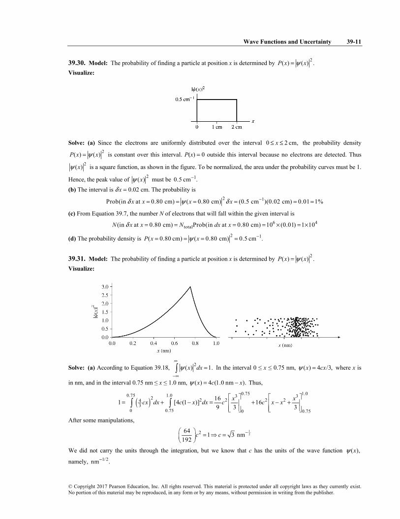
39.30. Model: The probability of finding a particle at position x is determined by 2( ) ( ) .P x xψ= Visualize:

Solve: (a) Since the electrons are uniformly distributed over the interval 0 2 cm,x≤ ≤ the probability density 2( ) ( )P x xψ= is constant over this interval. P(x) = 0 outside this interval because no electrons are detected. Thus

2( )xψ is a square function, as shown in the figure. To be normalized, the area under the probability curves must be 1.

Hence, the peak value of 2( )xψ must be 10.5 cm .− (b) The interval is δ x = 0.02 cm. The probability is

2 1Prob(in at 0 80 cm) ( 0 80 cm) (0 5 cm )(0 02 cm) 0 01 1%x x x xδ ψ δ −= . = = . = . . = . =

(c) From Equation 39.7, the number N of electrons that will fall within the given interval is 6 4

total(in at 0 80 cm) Prob(in at 0 80 cm) 10 (0 01) 1 10N x x N dx xδ = . = = . = × . = ×

(d) The probability density is 2 1( 0.80 cm) ( 0 80 cm) 0.5 cm .P x xψ −= = = . =


Solve: (a) According to Equation 39.18, 2( ) 1.x dxψ∞

−∞

=∫ In the interval 0 ≤ x ≤ 0.75 nm, ( ) 4 /3,x cxψ = where x is

in nm, and in the interval 0.75 nm ≤ x ≤ 1.0 nm, ( ) 4 (1.0 nm ).x c xψ = − Thus,

( )0 75 1 00 75 1.0 3 32 2 2 2 24

30 0.75 0 0 75

161 [4 (1 )] 169 3 3

x xcx dx c x dx c c x x. ..

.

⎡ ⎤ ⎡ ⎤= + − = + − +⎢ ⎥ ⎢ ⎥

⎢ ⎥ ⎢ ⎥⎣ ⎦ ⎣ ⎦∫ ∫

After some manipulations, 12264 1 3 nm

192c c −⎛ ⎞ = ⇒ =⎜ ⎟

⎝ ⎠

We did not carry the units through the integration, but we know that c has the units of the wave function ( ),xψ

namely, 1/2nm .−

39-12 Chapter 39


(b) The particle wave function is ( ) 4 / 3x xψ = for the interval 0 nm ≤ x ≤ 0.75 nm and ( ) 4 3(1 0 )x xψ = . − for the

interval 0.75 nm ≤ x ≤ 1.0 nm. Thus, 2 2( ) (16/3)x xψ = for 0 nm ≤ x ≤ 0.75 nm and 2 2( ) 48(1 )x xψ = − for 0.75 nm ≤ x

≤ 1.0 nm. 2( )xψ has units of 1nm .− The graph is shown on the previous page.

(c) The particle is most likely to be found at the points where 2( )xψ is a maximum. The dot picture is shown on the previous page. (d) The probability is

0 25 0 252 2

0 0 0 00 253

0 0

16Prob(0 0 nm 0 25 nm) ( )3

16 13 3 36

0 028

x x dx x dx

x

ψ. .

. ..

.

. ≤ ≤ . = =

⎡ ⎤= =⎢ ⎥

⎢ ⎥⎣ ⎦= .

∫ ∫


Solve: (a) Yes, because the area under the 2( )xψ curve is equal to 1. (b) There are two things to consider when drawing ( ).xψ First ( )xψ is an oscillatory function that changes sign every time it reaches zero. Second, ( )xψ must have the right shape. Each point on the ( )xψ curve is the square root

of the corresponding point on the 2( )xψ curve. The values 2 1( ) 1 cmxψ −= and 2 1( ) 0 cmxψ −= clearly give 1/2( ) 1 cmxψ −= ± and 1/2( ) 0 cm ,xψ −= respectively. But consider 0 5 cm,x = . where 2 1( ) 0 5 cm .xψ −= . Because

1/20 5 0 707, ( 0.5 cm) 0.707 cm .xψ −. = ± . = = ± This tells us that the ( )xψ curve is not linear but bows upward (or downward if we take the negative square root) over the interval 0 ≤ x ≤ 1 cm. Thus, ( )xψ has the shape shown in the above figure.



(c) δ x = 0.0010 cm is a very small interval, so we can use 2Prob(in at ) ( ) .x x x xδ ψ δ= The values of 2( )xψ can be read from Figure P39.32. Thus,

( ) 2 1

2 1

2 1

Prob in at 0 00 cm ( 0 00 cm) (0 00 cm )(0 0010 cm) 0 00

Prob(in at 0 50 cm) ( 0 50 cm) (0 50 cm )(0 0010 cm) 0 00050

Prob(in at 0 999 cm) ( 0 999 cm) (0 999 cm )(0 0010 cm) 0 009

x x x x

x x x x

x x x x

δ ψ δ

δ ψ δ

δ ψ δ

−

−

−

= . = = . = . . = .

= . = = . = . . = .

= . = = . = . . = . 99 0 0010≈ .

(d) The number N of electrons expected to land in the interval 0.3 cm 0.3 cm isx− ≤ ≤

( )total

0.30 cm24 4 11

20.30 cm

(in 0 30 cm 0 30 cm) Prob(in 0 30 cm 0 30 cm)

(1 10 ) ( ) (1 10 ) 2 0 30 cm 0 30 cm

900

N x N x

x dxψ −

−

− . ≤ ≤ . = − . ≤ ≤ .

⎡ ⎤= × = × × × . × .⎢ ⎥⎣ ⎦

=

∫

39.33. Model: The probability of finding a particle at position x is determined by the probability density 2( ) ( ) .P x xψ= Solve: (a) The probability density extends from 4 cm to 4 cm.− + The area under the P(x)-versus-x graph must be unity, so

4.0 cm2 1

4.0 cm

1 ( ) (4 0 cm) 0 25 cmx dx a aψ −

−

= = . ⇒ = .∫

(b) The particle is most likely to be found at a position where 2( )xψ is a maximum. This will occur at 0 cmx = because P(x) has its greatest value at x = 0.0 cm. (c) 75% of the area under the curve occurs between 2.0 cmx = − and 2.0 cm, so the range is 2.0 cm 2.0 cm.x− ≤ ≤ (d)

39.34. Model: The probability of finding a particle at position x is determined by the probability density 2( ) ( ) .P x xψ= Solve: (a) The wave function is a straight line passing through the origin such that it is +c at x = +4 mm and −c at x = –4 mm. That is, the wave function is

( ) /4x cxψ =

where x is in mm and c is in 1/2mm .− Note that the units of c must be that of ( ).xψ Because the total probability must be unity, we have

44 4 2 32 2 2 2 2 2 1/2

4 0 0

2 8 31 ( ) ( /16) 2 ( /16) mm16 3 3 8c xx dx c x dx c x dx c cψ

∞−

−∞ −

⎡ ⎤= = = = = ⇒ =⎢ ⎥

⎢ ⎥⎣ ⎦∫ ∫ ∫

(b) From part (a), we have 2

2 2 2 2 13( ) /16 3 /128 (mm )128

xx c x xψ −= = =

39-14 Chapter 39


A 2( )xψ -versus-x graph is shown in the figure below.

(c) The particle is most likely to be found at the positions where 2( )xψ is a maximum. The graph above gives a dot picture of the first few particles.

(d) 2 02.0 mm 2.0 2 3

2

2.0 mm 0 0

3 3Prob( 2 0 mm 2 0 mm) ( ) 2 2 0 125 0 13128 128 3

x xx x dx dxψ.

−

⎡ ⎤⎛ ⎞− . ≤ ≤ . = = = = . ≈ .⎢ ⎥⎜ ⎟⎝ ⎠ ⎢ ⎥⎣ ⎦

∫ ∫

39.35. Model: The probability of finding a particle at position x is determined by the probability density 2( ) ( ) .P x xψ=

Solve: (a) The wave function / / nm( ) (1.414 nm ) xx eψ −1 2 − (1.0 )= changes over a length scale of ~1 nm. The distance 0.010 nmxδ = is very small compared to 1 nm. So we can use

2

1/2 1 2

2

Prob(in 0.010 nm at 1.0 nm) ( 1.0 nm)

[(1.414 nm ) ] (0.010 nm)

2 (0.010) 0.0027 0.27%

x x x x

e

e

δ ψ δ− −

−

= = = =

=

= = =


Solve: (a) Normalization of the wave function requires that 2( ) 1.x dxψ∞

−∞

=∫ Therefore,

11 32 2 2 2 1/2

1 1

4 31 (1 ) 0 87 cm3 3 4xc x dx c x c c −

− −

⎡ ⎤= − = − = ⇒ = = .⎢ ⎥

⎢ ⎥⎣ ⎦∫

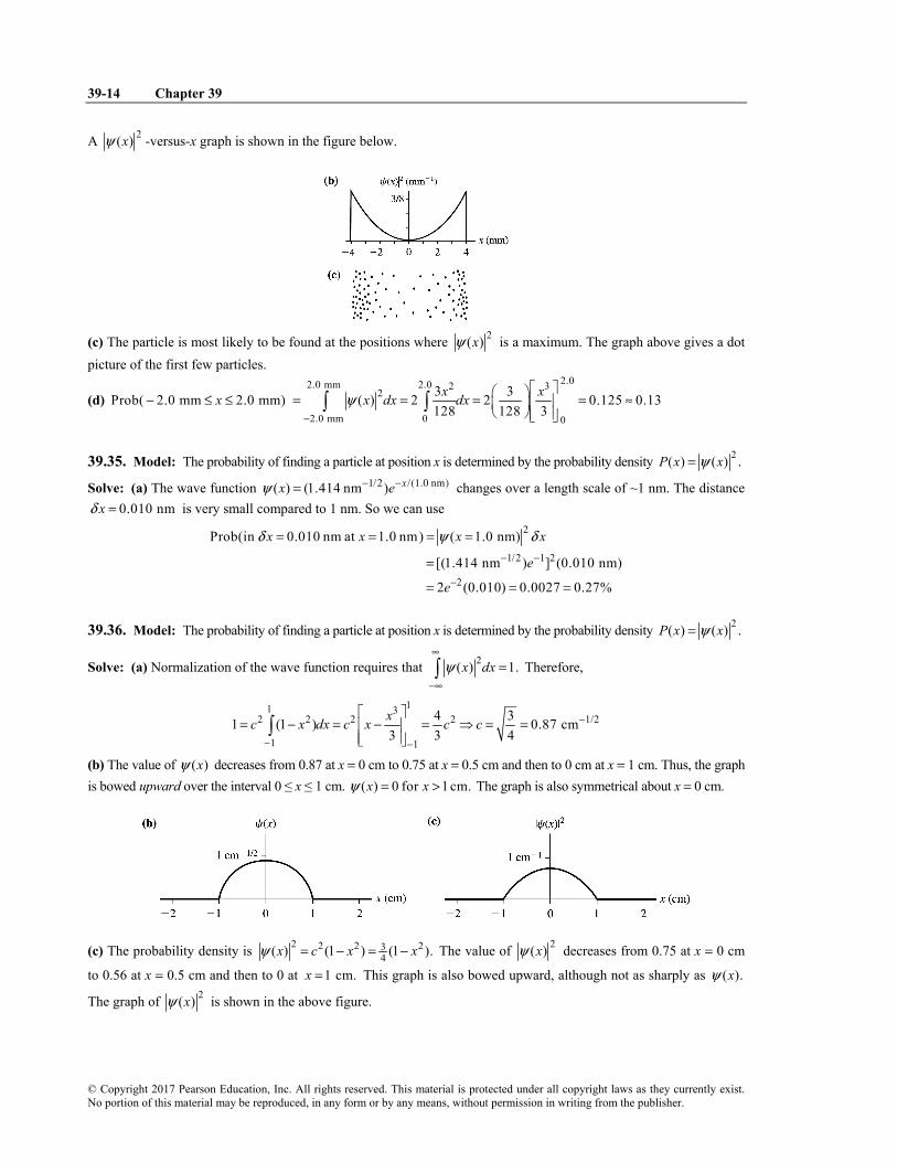
(b) The value of ( )xψ decreases from 0.87 at x = 0 cm to 0.75 at x = 0.5 cm and then to 0 cm at x = 1 cm. Thus, the graph is bowed upward over the interval 0 ≤ x ≤ 1 cm. ( ) 0 for 1 cm.x xψ = > The graph is also symmetrical about x = 0 cm.

(c) The probability density is 2 2 2 234( ) (1 ) (1 ).x c x xψ = − = − The value of 2( )xψ decreases from 0.75 at x = 0 cm

to 0.56 at x = 0.5 cm and then to 0 at 1 cm.x = This graph is also bowed upward, although not as sharply as ( ).xψ

The graph of 2( )xψ is shown in the above figure.



(d) The number of electrons is

total(in 0 00 cm 0 50 cm) Prob(in 0 00 cm 0 50 cm)N x N x. ≤ ≤ . = . ≤ ≤ .

0 500.50 cm 0.50 32 2

0.00 cm 0.00 0 00

3 3Prob(in 0 00 cm 0 50 cm) ( ) (1 ) 0 3444 4 3

xx x dx x dx xψ.

.

⎡ ⎤. ≤ ≤ . = = − = − = .⎢ ⎥

⎢ ⎥⎣ ⎦∫ ∫

Thus, the number of electrons detected in the interval 0 cm ≤ x ≤ 0.5 cm is 310,000 0.344 3440 3.4 10 .× = ≈ ×


Solve: (a) Normalization of the wave function requires that 2( ) 1.x dxψ∞

−∞

=∫ By changing variables to θ = 2πx/L, we

find 2

2 2 2 2 2

0 0

2 2 21 sin sin2 2 2

L x L Lc dx c d c cL L

ππ πθ θπ π

⎛ ⎞ ⎛ ⎞⎛ ⎞= = = ⇒ =⎜ ⎟ ⎜ ⎟⎜ ⎟⎝ ⎠ ⎝ ⎠⎝ ⎠∫ ∫

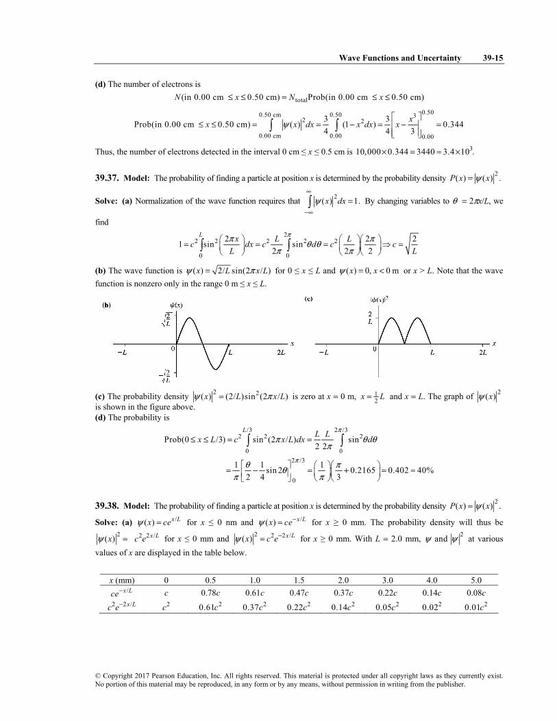
(b) The wave function is ( ) 2/ sin(2 / )x L x Lψ π= for 0 ≤ x ≤ L and ( ) 0, 0 mx xψ = < or x > L. Note that the wave function is nonzero only in the range 0 m ≤ x ≤ L.

(c) The probability density 2 2( ) (2/ )sin (2 / )x L x Lψ π= is zero at x = 0 m, 12x L= and x = L. The graph of 2( )xψ

is shown in the figure above. (d) The probability is

/3 2 /32 2 2

0 02 /3

0

Prob(0 /3) sin (2 / ) sin2 2

1 1 1sin 2 0 2165 0 402 40%2 4 3

L L Lx L c x L dx dπ

π

π θ θπ

θ πθπ π

≤ ≤ = =

⎡ ⎤ ⎛ ⎞⎛ ⎞= − = + . = . ≈⎜ ⎟⎜ ⎟⎢ ⎥⎣ ⎦ ⎝ ⎠⎝ ⎠

∫ ∫


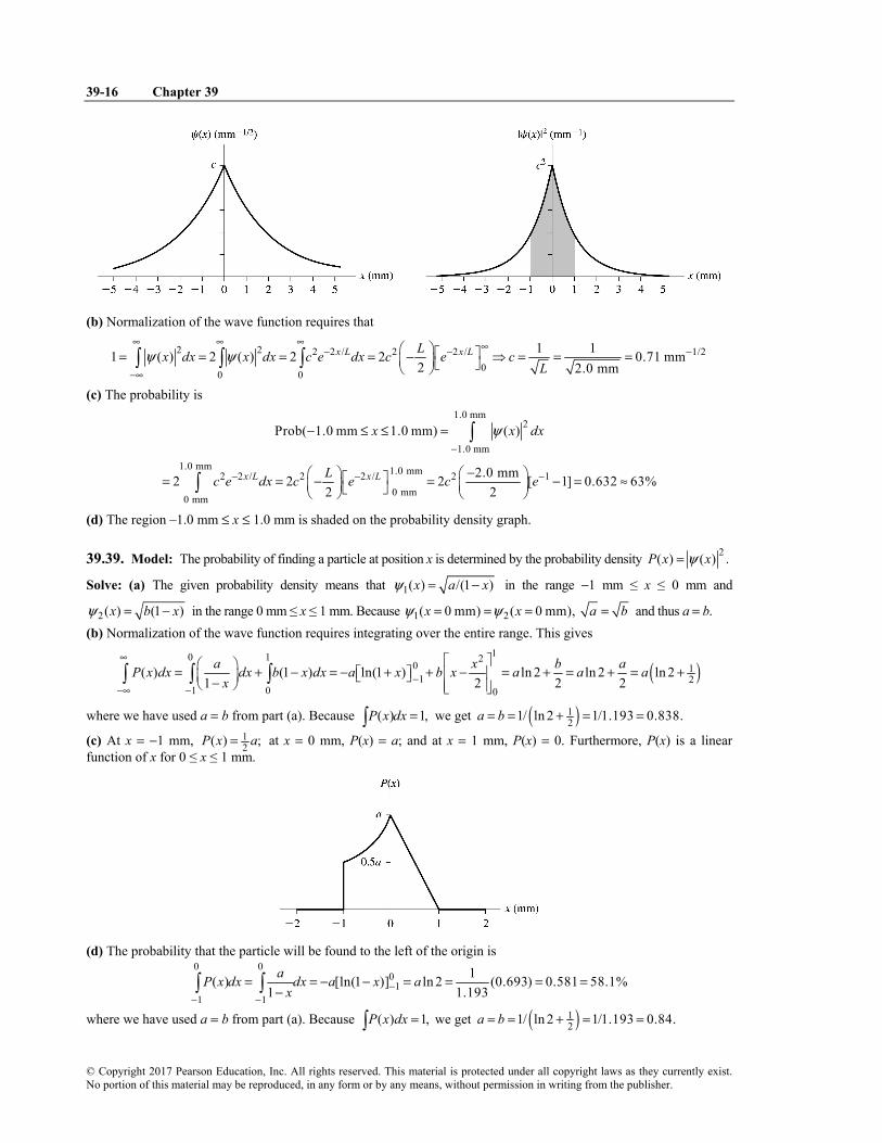
Solve: (a) /( ) x Lx ceψ = for x ≤ 0 nm and /( ) x Lx ceψ −= for x ≥ 0 mm. The probability density will thus be 2( )xψ = 2 2 /x Lc e for x ≤ 0 mm and 2 2 2 /( ) x Lx c eψ −= for x ≥ 0 mm. With L = 2.0 mm, 2andψ ψ at various

values of x are displayed in the table below.

x (mm) 0 0.5 1.0 1.5 2.0 3.0 4.0 5.0 /x Lce− c 0.78c 0.61c 0.47c 0.37c 0.22c 0.14c 0.08c

2 2 /x Lc e− 2c 20.61c 20.37c 20.22c 20.14c 20.05c 20.02 20.01c

39-16 Chapter 39


(b) Normalization of the wave function requires that

2 2 2 2 / 2 2 / 1/20

0 0

1 11 ( ) 2 ( ) 2 2 0 71 mm2 2 0 mm

x L x LLx dx x dx c e dx c e cL

ψ ψ∞ ∞ ∞ ∞− − −

−∞

⎛ ⎞ ⎡ ⎤= = = = − ⇒ = = = .⎜ ⎟ ⎣ ⎦ .⎝ ⎠∫ ∫ ∫

(c) The probability is 1.0 mm

2

1.0 mm

1.0 mm 1 0 mm2 2 / 2 2 / 2 10 mm

0 mm

Prob( 1.0 mm 1.0 mm) ( )

2 0 mm2 2 2 [ 1] 0 632 63%2 2

x L x L

x x dx

Lc e dx c e c e

ψ−

.− − −

− ≤ ≤ =

− .⎛ ⎞ ⎛ ⎞⎡ ⎤= = − = − = . ≈⎜ ⎟ ⎜ ⎟⎣ ⎦⎝ ⎠ ⎝ ⎠

∫

∫

(d) The region –1.0 mm ≤ x ≤ 1.0 mm is shaded on the probability density graph.


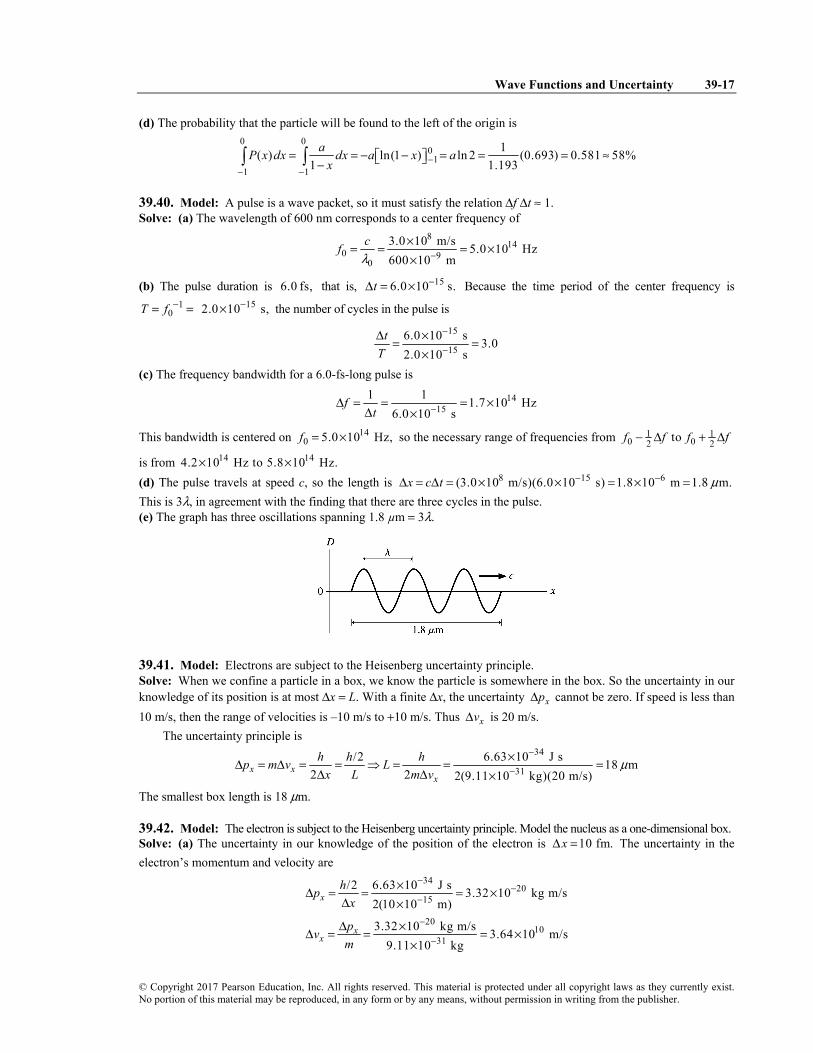
Solve: (a) The given probability density means that 1( ) /(1 )x a xψ = − in the range −1 mm ≤ x ≤ 0 mm and

2( ) (1 )x b xψ = − in the range 0 mm ≤ x ≤ 1 mm. Because 1 2( 0 mm) ( 0 mm),x xψ ψ= = = a b= and thus a = b. (b) Normalization of the wave function requires integrating over the entire range. This gives

( )10 1 2

0 11 2

1 0 0

( ) (1 ) ln(1 ) ln 2 ln 2 ln 21 2 2 2

a x b aP x dx dx b x dx a x b x a a ax

∞

−−∞ −

⎡ ⎤⎛ ⎞= + − = − + + − = + = + = +⎡ ⎤ ⎢ ⎥⎜ ⎟ ⎣ ⎦−⎝ ⎠ ⎢ ⎥⎣ ⎦∫ ∫ ∫

where we have used a = b from part (a). Because ( ) 1,P x dx =∫ we get ( )121/ ln 2 1/1 193 0 838.a b= = + = . = .

(c) At x = −1 mm, 12( ) ;P x a= at x = 0 mm, P(x) = a; and at x = 1 mm, P(x) = 0. Furthermore, P(x) is a linear

function of x for 0 ≤ x ≤ 1 mm.

(d) The probability that the particle will be found to the left of the origin is 0 0

01

1 1

1( ) [ln(1 )] ln 2 (0 693) 0 581 58 1%1 1 193

aP x dx dx a x ax −

− −

= = − − = = . = . = .− .∫ ∫

where we have used a = b from part (a). Because ( ) 1,P x dx =∫ we get ( )121/ ln 2 1/1 193 0 84a b= = + = . = . .



(d) The probability that the particle will be found to the left of the origin is 0 0

01

1 1

1( ) ln(1 ) ln 2 (0 693) 0 581 58%1 1 193

aP x dx dx a x ax −

− −

= = − − = = . = . ≈⎡ ⎤⎣ ⎦− .∫ ∫

39.40. Model: A pulse is a wave packet, so it must satisfy the relation Δf Δt ≈ 1. Solve: (a) The wavelength of 600 nm corresponds to a center frequency of

814

0 90

3 0 10 m/s 5 0 10 Hz600 10 m

cfλ −

. ×= = = . ××

(b) The pulse duration is 6.0 fs, that is, 156 0 10 s.t −Δ = . × Because the time period of the center frequency is 1

0T f −= = 152 0 10 s,−. × the number of cycles in the pulse is

15

156 0 10 s 3 02 0 10 s

tT

−

−Δ . ×= = .

. ×

(c) The frequency bandwidth for a 6.0-fs-long pulse is

1415

1 1 1 7 10 Hz6 0 10 s

ft −Δ = = = . ×

Δ . ×

This bandwidth is centered on 140 5 0 10 Hz,f = . × so the necessary range of frequencies from 1 1

0 02 2tof f f f− Δ + Δ

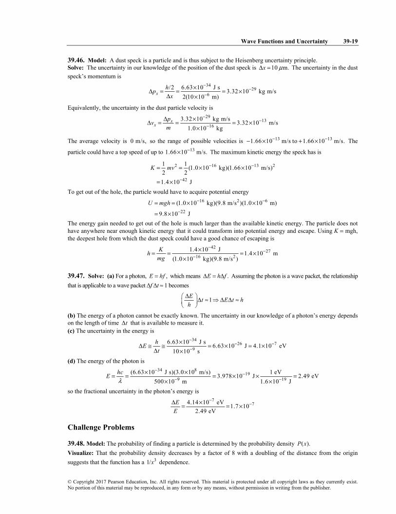
is from 14 144.2 10 Hz to 5.8 10 Hz.× × (d) The pulse travels at speed c, so the length is 8 15 6(3.0 10 m/s)(6.0 10 s) 1.8 10 m m.x c t μ− −Δ = Δ = × × = × =1.8 This is 3λ, in agreement with the finding that there are three cycles in the pulse. (e) The graph has three oscillations spanning 1.8 µm = 3λ.

39.41. Model: Electrons are subject to the Heisenberg uncertainty principle. Solve: When we confine a particle in a box, we know the particle is somewhere in the box. So the uncertainty in our knowledge of its position is at most Δx = L. With a finite Δx, the uncertainty xpΔ cannot be zero. If speed is less than 10 m/s, then the range of velocities is –10 m/s to +10 m/s. Thus xvΔ is 20 m/s.

The uncertainty principle is 34

31/2 6 63 10 J s 18 m

2 2 2(9 11 10 kg)(20 m/s)x xx

h h hp m v Lx L m v

μ−

−. ×Δ = Δ = = ⇒ = = =

Δ Δ . ×

The smallest box length is 18 μm.

39.42. Model: The electron is subject to the Heisenberg uncertainty principle. Model the nucleus as a one-dimensional box. Solve: (a) The uncertainty in our knowledge of the position of the electron is 10 fmxΔ = . The uncertainty in the electron’s momentum and velocity are

3420

15

2010

31

/2 6 63 10 J s 3 32 10 kg m/s2(10 10 m)

3 32 10 kg m/s 3 64 10 m/s9 11 10 kg

x

xx

hpx

pvm

−−

−

−

−

. ×Δ = = = . ×Δ ×

Δ . ×Δ = = = . ×. ×

39-18 Chapter 39


The range of possible velocities is 10 101.82 10 m/s to 1.82 10 m/s,− × + × so the range of speeds is from 0 m/s to 101.82 10 m/s.×

(b) The minimum range of speeds for an electron confined to a nucleus exceeds the speed of light, so it is not possible.

39.43. Model: The alpha particle is in a one-dimensional box. Assume our uncertainty in position is 15 fm.x LΔ = = Visualize: Use the uncertainty principle, ( )( ) /2.x mv hΔ Δ ≈

Solve: (a)

346

276.63 10 J s 3.3 10 m/s

2 2(4.0 u)(1.661 10 kg/u)(15 fm)xhvmL

−

−× ⋅Δ = = = ××

This is the range of velocities in the x-direction, so the maximum likely speed is ½ of this, or 61.7 10 m/s.× (b) The number of reflections will be this maximum speed divided by the diameter of the nucleus.

6201 1.7 10 m/s 1.1 10 reflections/s

15 fmvf

T x×= = = = ×

Δ

Assess: Quantum tunneling (see next chapter) is also important in alpha decay.

39.44. Model: The electron is subject to the Heisenberg uncertainty principle. Model the nucleus as a one-dimensional box. Solve: (a) The uncertainty in our knowledge of the position of the electron is 10 fmxΔ = . The uncertainty in the electron’s momentum and velocity are

3420

15

2010

31

/2 6 63 10 J s 3 32 10 kg m/s2(10 10 m)

3 32 10 kg m/s 3 64 10 m/s9 11 10 kg

x

xx

hpx

pvm

−−

−

−

−

. ×Δ = = = . ×Δ ×

Δ . ×Δ = = = . ×. ×

The range of possible velocities is 10 101.82 10 m/s to 1.82 10 m/s,− × + × so the range of speeds is from 0 m/s to 101.82 10 m/s.×

(b) The minimum range of speeds for an electron confined to a nucleus exceeds the speed of light, so it is not possible.

39.45. Model: The soot particle is subject to the Heisenberg uncertainty principle. Ignore air resistance so the particle is in free fall. Visualize: We are given the radius of a soot particle 7.5 nm.R =

Solve: First find the mass of a soot particle. 3 3 3 214 4

3 3(1200 kg/m ) (7.5 nm) 2.12 10 kgm V Rρ ρ π π −= = = = ×

There is uncertainty in the x velocity and position with xΔ being the diameter of the hole.

347

216.63 10 J s 3.13 10 m/s

2 2(2.12 10 kg)(0.50 m)xhv

m x μ

−−

−× ⋅Δ = = = ×

Δ ×

This is the range of velocities in the x-direction, so the maximum likely speed is ½ of this, or 71.56 10 m/s.−× We find how long it takes to travel the radius of the detector circle in the x-direction at this speed.

71000 nm 6.397 s

1.56 10 m/st −Δ = =

×

Now d is the free-fall distance in that time interval.

2 2 21 1( ) (9.8 m/s )(6.397 s) 200 m2 2

d g t= Δ = =

Assess: The spreading isn’t very much, but soot particles have much more mass than an atom.



39.46. Model: A dust speck is a particle and is thus subject to the Heisenberg uncertainty principle. Solve: The uncertainty in our knowledge of the position of the dust speck is 10 m.x μΔ = The uncertainty in the dust speck’s momentum is

3429

6/2 6 63 10 J s 3 32 10 kg m/s

2(10 10 m)xhp

x

−−

−. ×Δ = = = . ×

Δ ×

Equivalently, the uncertainty in the dust particle velocity is 29

1316

3 32 10 kg m/s 3 32 10 m/s1 0 10 kg

xx

pvm

−−

−Δ . ×Δ = = = . ×

. ×

The average velocity is 0 m/s, so the range of possible velocities is 13 131.66 10 m/s to 1.66 10 m/s.− −− × + × The

particle could have a top speed of up to 131.66 10 m/s.−× The maximum kinetic energy the speck has is

2 16 13 2

42

1 1 (1 0 10 kg)(1 66 10 m/s)2 21 4 10 J

K mv − −

−

= = . × . ×

= . ×

To get out of the hole, the particle would have to acquire potential energy 16 2 6

22

(1 0 10 kg)(9 8 m/s )(1 0 10 m)

9 8 10 J

U mgh − −

−

= = . × . . ×

= . ×

The energy gain needed to get out of the hole is much larger than the available kinetic energy. The particle does not have anywhere near enough kinetic energy that it could transform into potential energy and escape. Using K = mgh, the deepest hole from which the dust speck could have a good chance of escaping is

4227

16 21 4 10 J 1 4 10 m

(1 0 10 kg)(9 8 m/s )Kh

mg

−−

−. ×= = = . ×

. × .

39.47. Solve: (a) For a photon, ,E hf= which means .E h fΔ = Δ Assuming the photon is a wave packet, the relationship that is applicable to a wave packet Δf Δt ≈ 1 becomes

1E t E t hh

Δ⎛ ⎞Δ ≈ ⇒ Δ Δ ≈⎜ ⎟⎝ ⎠

(b) The energy of a photon cannot be exactly known. The uncertainty in our knowledge of a photon’s energy depends on the length of time tΔ that is available to measure it. (c) The uncertainty in the energy is

3426 7

96 63 10 J s 6 63 10 J 4 1 10 eV

10 10 shEt

−− −

−. ×Δ ≅ ≅ = . × = . ×

Δ ×

(d) The energy of the photon is 34 8

199 19

(6 63 10 J s)(3 0 10 m/s) 1 eV3 978 10 J 2 49 eV500 10 m 1 6 10 J

hcEλ

−−

− −. × . ×= = = . × × = .

× . ×

so the fractional uncertainty in the photon’s energy is 7

74 14 10 eV 1 7 102 49 eV

EE

−−Δ . ×= = . ×

.

Challenge Problems

39.48. Model: The probability of finding a particle is determined by the probability density ( ).P x Visualize: That the probability density decreases by a factor of 8 with a doubling of the distance from the origin suggests that the function has a 31/x dependence.

39-20 Chapter 39


Solve: The conditions at 1 mmx = give the following probability density.

23

0 1 mm( ) ( )

/ 1 mm

xP x x

c x xψ

<⎧⎪= = ⎨≥⎪⎩

We find c from the normalization condition.

2 2 21 mm3 3

1 mm

1 1 [ ] [0 1 mm ] 1 2 mm2 2

c cdx c dx c x cx x

∞ ∞− ∞ −

−∞

⎛ ⎞= = − ⇒ − − = ⇒ =⎜ ⎟⎝ ⎠∫ ∫

Now we integrate from 2 mm to 4 mm.

4 mm2 2 4 mm 2

2 mm3 2 2 2 22 mm

1 1 1 1 1 1(2 mm) [ ] ( 1 mm ) 19%2 (4 mm) (2 mm) 2 4

c dx xx

− ⎡ ⎤⎛ ⎞= − ⇒ − − = − =⎢ ⎥⎜ ⎟⎝ ⎠ ⎢ ⎥⎣ ⎦

∫

Assess: There is a 75% chance of finding the particle between 1 mm and 2 mm, so it seems reasonable that there is a 19% chance between 2 mm and 4 mm.

39.49. Model: The probability of finding a particle at position x is determined by the probability density 2( ) ( ) .P x xψ= Solve: We first need to see if the wave function is normalized:

2 12 2

1 1( ) tan 12 2( )

b b xx dx dxb bx b

π πψπ ππ

∞∞ ∞−

−∞−∞ −∞

⎡ ⎤⎡ ⎤ ⎛ ⎞= = = − − =⎢ ⎥⎜ ⎟⎢ ⎥+ ⎣ ⎦ ⎝ ⎠⎣ ⎦∫ ∫

The function was already normalized. The probability is

2 12 2

1 1

1Prob( ) ( ) tan( )

1 1[tan (1) tan ( 1)] 50%2

bb b

bb b

b dx b xb x b x dxb bx b

ψπ π

π

−

−− −

− −

⎡ ⎤− ≤ ≤ = = = ⎢ ⎥+ ⎣ ⎦

= − − = =

∫ ∫

39.50. Model: The probability of finding a particle at position x is determined by the probability density 2( ) ( ) .P x xψ= Solve: (a)

2

2

( ) 1 mm 0 mm(1 )

(1 ) 0 mm 1 mm0 elsewhere

bx xx

c x x

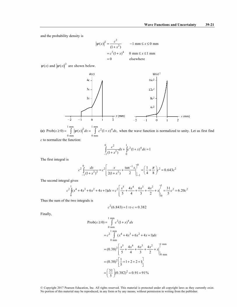
ψ = − ≤ ≤+

= + ≤ ≤=

Because the value of the wave function must be the same at x = 0 (note that the x = 0 mm point is covered in both the left ( 1 mm 0 mm)x− ≤ ≤ and the right (0 mm 1 mm)x≤ ≤ parts of the wave function),

22 (1 0 mm)

1 (0 mm)b c

b c

= ++

=

(b) So the wave function is

2

2

( ) 1 mm 0 mm(1 )


cx xx

c x x

ψ = − ≤ ≤+

= + ≤ ≤=



and the probability density is 2

22

2 4

( ) 1 mm 0 mm(1 )


cx xx

c x x

ψ = − ≤ ≤+

= + ≤ ≤=

2( ) and ( ) are shown belowx xψ ψ .

(c) 1 mm 1 mm

2 2 4

0 mm 0 mm

Prob( 0) ( ) (1 ) ,x x dx c x dxψ≥ = = +∫ ∫ when the wave function is normalized to unity. Let us first find

c to normalize the function: 0 12

2 42

1 0

(1 ) 1(1 )

c dx c x dxx−

+ + =+∫ ∫

The first integral is 00 1

2 2 2 22 2 2

1 1

tan 1 0 6432 4 8(1 ) 2(1 )

dx x xc c c cx x

π−

− −

⎡ ⎤ ⎛ ⎞= + = + = .⎢ ⎥ ⎜ ⎟+ + ⎝ ⎠⎢ ⎥⎣ ⎦∫

The second integral gives 11 5 4 3 2

2 4 3 2 2 2 2

0 0

4 6 4 31( 4 6 4 1) 6 205 4 3 2 5x x x xc x x x x dx c x c c

⎡ ⎤+ + + + = + + + + = = .⎢ ⎥

⎢ ⎥⎣ ⎦∫

Thus the sum of the two integrals is 2(6 843) 1 0 382c c. = ⇒ = .

Finally, 1 mm

2 4

0 mm1 mm

2 4 3 2

0 mm1 mm5 4 3 2

2

0 mm

2

2

Prob( 0) (1 )

( 4 6 4 1)

4 6 4(0 38)5 4 3 2

1(0 38) 1 2 2 15

31 (0 382) 0 91 91%5

x c x dx

c x x x x dx

x x x x x

≥ = +

= + + + +

⎡ ⎤= . + + + +⎢ ⎥

⎢ ⎥⎣ ⎦

⎡ ⎤= . + + + +⎢ ⎥⎣ ⎦⎛ ⎞= . = . =⎜ ⎟⎝ ⎠

∫

∫

39-22 Chapter 39



Solve: (a) The normalization condition demands 2( ) 1.x dxψ∞

−∞

=∫ Hence,

1 0 1 12 2 22 2 2 2 2 2

2 2 21 0 1 0 1

132 2 2 2

10

2 2 1

1 2 32 2 2 13 3 8

c c cdx c x dx c x dx dx c x dx dxx x x

xc c c c cx

− ∞ ∞

−∞ −

∞

+ + + = + =

⎡ ⎤ ⎡ ⎤+ − = + = ⇒ =⎢ ⎥ ⎢ ⎥⎣ ⎦⎢ ⎥⎣ ⎦

∫ ∫ ∫ ∫ ∫ ∫

(b)

(c) The probability density is

( ) ( )2 222

3 3( ) 1 nm ( ) 1 nm8 8

x x x x xx

ψ ψ⎛ ⎞ ⎛ ⎞= ≤ = ≥⎜ ⎟ ⎜ ⎟⎝ ⎠ ⎝ ⎠

The figure above shows the 2( ) - versus- graph.x xψ (d) The probability is

1.0 nm 1.0 nm2 2 2 2 2

1.0 nm 0.0 nm

2 2 3Prob( 1 0 nm 1 0 nm) 2 25%3 3 8

x c x dx c x dx c−

⎛ ⎞− . ≤ ≤ . = = = = =⎜ ⎟⎝ ⎠∫ ∫

The number of electrons detected is 6 5(0.25)(10 ) 2.5 10 .= ×

Date post:	18-Dec-2021
Category:	Documents
Upload:	others
View:	3 times
Download:	0 times

M39 KNIG2461 04 ISM C39 - media.physicsisbeautiful.com

Documents