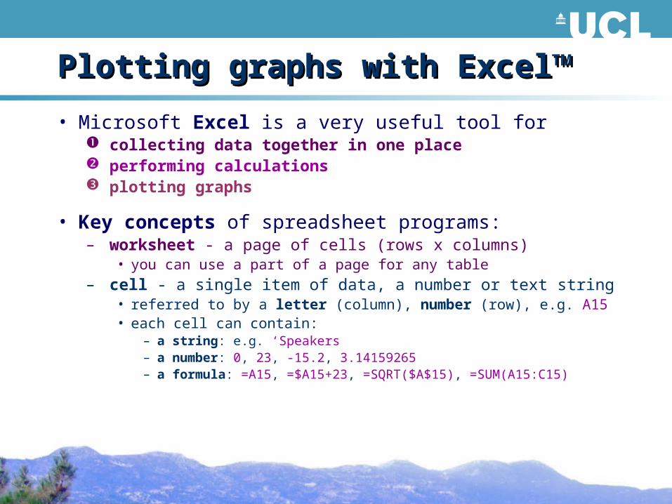
MA in English Linguistics Experimental design and statistics II

MA in English LinguisticsMA in English LinguisticsExperimental design and statistics IIExperimental design and statistics II

Sean WallisSurvey of English Usage

University College London

[email protected]

OutlineOutline

• Plotting data with Excel™

• The idea of a confidence interval

• Binomial Normal Wilson

• Interval types– 1 observation

– The difference between 2 observations

• From intervals to significance tests

Plotting graphs with ExcelPlotting graphs with Excel™™

• Microsoft Excel is a very useful tool for collecting data together in one place performing calculations plotting graphs

• Key concepts of spreadsheet programs:– worksheet - a page of cells (rows x columns)

• you can use a part of a page for any table– cell - a single item of data, a number or text string

• referred to by a letter (column), number (row), e.g. A15• each cell can contain:

– a string: e.g. ‘Speakers– a number: 0, 23, -15.2, 3.14159265– a formula: =A15, =$A15+23, =SQRT($A$15), =SUM(A15:C15)

Plotting graphs with ExcelPlotting graphs with Excel™™

• Importing data into Excel:– Manually, by typing– Exporting data from ICECUP

• Manipulating data in Excel to make it useful:– Copy, paste: columns, rows, portions of tables– Creating and copying functions– Formatting cells

• Creating and editing graphs:– Several different types (bar chart, line chart, scatter, etc)– Can plot confidence intervals as well as points

• You can download a useful spreadsheet for performing statistical tests:

– www.ucl.ac.uk/english-usage/statspapers/2x2chisq.xls

Recap: the idea of probabilityRecap: the idea of probability

• A way of expressing chance0 = cannot happen1 = must happen

• Used in (at least) three ways last weekP = true probability (rate) in the populationp = observed probability in the sample = probability of p being different from P– sometimes called probability of error, pe– found in confidence intervals and significance

tests

The idea of a confidence The idea of a confidence intervalinterval• All observations are imprecise

– Randomness is a fact of life– Our abilities are finite:

• to measure accurately or • reliably classify into types

• We need to express caution in citing numbers

• Example (from Levin 2013):– 77.27% of uses of think in 1920s data

have a literal (‘cogitate’) meaning





• Example (from Levin 2013):– 77.27% of uses of think in 1920s data


Really? Not 77.28, or 77.26?





• Example (from Levin 2013):– 77% of uses of think in 1920s data






• Example (from Levin 2013):– 77% of uses of think in 1920s data


Sounds defensible. But how confident can we be in this number?





• Example (from Levin 2013):– 77% (66-86%*) of uses of think in 1920s

data have a literal (‘cogitate’) meaning





• Example (from Levin 2013):– 77% (66-86%*) of uses of think in 1920s

data have a literal (‘cogitate’) meaning

Finally we have a credible range of values - needs a footnote* to explain how it was calculated.

Binomial Binomial Normal Normal Wilson Wilson

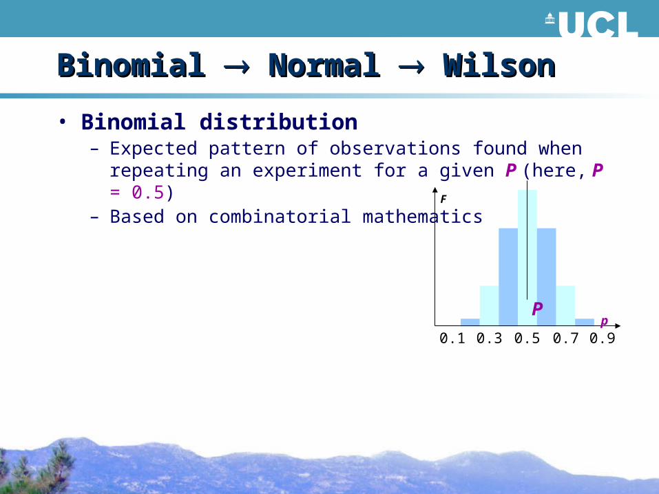
• Binomial distribution– Expected pattern of observations found when

repeating an experiment for a given P (here, P = 0.5)– Based on combinatorial mathematics

p

F

0.50.30.1 0.7 0.9

P




– Other values of P have differentexpected distribution patterns

p

F

0.50.30.1 0.7 0.9

P

0.3 0.1 0.05




• Binomial Normal– Simplifies the Binomial distribution

(tricky to calculate) to two variables:• mean P

– P is the most likely value

• standard deviation S– S is a measure of spread

p

F

0.50.30.1 0.7 0.9

P

S


• Binomial distribution

• Binomial Normal– Simplifies the Binomial distribution

(tricky to calculate) to two variables:• mean P• standard deviation S

• Normal Wilson– The Normal distribution predicts

observations p given a populationvalue P

– We want to do the opposite: predict the true population value P from an observation p

– We need a different interval, the Wilson score interval

p

F

0.50.30.1 0.7 0.9

P

Binomial Binomial Normal Normal

• Any Normal distribution can be defined by only two variables and the Normal function z

z . S z . S

F

– With more data in the experiment, S will be smaller

p0.50.30.1 0.7

population

mean P

standard deviationS = P(1 – P) / n



z . S z . S

F

2.5% 2.5%

population

mean P

– 95% of the curve is within ~2 standard deviations of the expected mean


p0.50.30.1 0.7

95%

– the correct figure is 1.95996!

= the critical value of z for an error level of 0.05.



z . S z . S

F

2.5% 2.5%

population

mean P

– 95% of the curve is within ~2 standard deviations of the expected mean


p0.50.30.1 0.7

95%

– The ‘tail areas’

– For a 95% interval, total 5%

The single-sample The single-sample zz test...test...

• Is an observation p > z standard deviations from the expected (population) mean P?

z . S z . S

F

P

p0.50.30.1 0.7

observation p• If yes, p is

significantly different from P

2.5% 2.5%

...gives us a “confidence ...gives us a “confidence interval”interval”• The interval about p is called the

Wilson score interval (w–, w+)• This interval

reflects the Normal interval about P:

• If P is at the upper limit of p,p is at the lower limit of P

(Wallis, 2013)

F

P2.5% 2.5%

p

w+

observation p

w–

0.50.30.1 0.7

...gives us a “confidence ...gives us a “confidence interval”interval”• The Wilson score interval (w–, w+)

has a difficult formula to remember

F

P2.5% 2.5%

p

w+

observation p

w–

0.50.30.1 0.7

s' = p(1 – p)/n + z²/4n²

p' = p + z²/2n

1 + z²/n

1 + z²/n

(w–, w+) = (p' – s', p' + s')

...gives us a “confidence ...gives us a “confidence interval”interval”• The Wilson score interval (w–, w+)

has a difficult formula to remember

F

P2.5% 2.5%

p

w+

observation p

w–

0.50.30.1 0.7

• You do not need to know this formula!

• You can use the 2x2 spreadsheet!

s' = p(1 – p)/n + z²/4n²

p' = p + z²/2n

1 + z²/n

1 + z²/n

(w–, w+) = (p' – s', p' + s')

– www.ucl.ac.uk/english-usage/statspapers/2x2chisq.xls

An example: uses of An example: uses of thinkthink

• Magnus Levin (2013) examined uses of think in the TIME corpus in three time periods– This is the graph we

created in ExcelWilson intervals without continuity correction

0

0.1

0.2

0.3

0.4

0.5

0.6

0.7

0.8

0.9

1

1920s 1960s 2000s

‘cogitate’

‘intend’

quotative

interpretative

– http://corplingstats.wordpress.com/2012/04/03/plotting-confidence-intervals/



created in Excel

– Not an alternation study• Categories are not

“choices”– The graph plots the

probability of readingdifferent uses of theword think (given thewriter used the word)

Wilson intervals without continuity correction

0

0.1

0.2

0.3

0.4

0.5

0.6

0.7

0.8

0.9

1

1920s 1960s 2000s

‘cogitate’

‘intend’

quotative

interpretative




created in Excel– Has Wilson score

intervals for eachpoint


0

0.1

0.2

0.3

0.4

0.5

0.6

0.7

0.8

0.9

1

1920s 1960s 2000s

‘cogitate’

‘intend’

quotative

interpretative




created in Excel– Has Wilson score

intervals for eachpoint

– It is easy to spot whereintervals overlap

• A quick test forsignificant difference


0

0.1

0.2

0.3

0.4

0.5

0.6

0.7

0.8

0.9

1

1920s 1960s 2000s

‘cogitate’

‘intend’

quotative

interpretative

– http://corplingstats.wordpress.com/2012/08/14/plotting-confidence-intervals-2/


• Magnus Levin (2013) examined uses of think in the TIME corpus in three time periods– Wilson score intervals

for each point– It is easy to spot where

intervals overlap• A quick test for

significant difference

– No overlap = significant– Overlaps point = ns– Otherwise test fully


0

0.1

0.2

0.3

0.4

0.5

0.6

0.7

0.8

0.9

1

1920s 1960s 2000s

‘cogitate’

‘intend’

quotative

interpretative


A quick test for significant A quick test for significant differencedifference• No overlap = significant

• Overlaps point = ns

• Otherwise test fully

0.5

0.6

0.7

0.8


p1

p2

w1–

w1+

w2–

w2+

A quick test for significant A quick test for significant differencedifference• No overlap = significant

• Overlaps point = ns

• Otherwise test fully

0.5

0.6

0.7

0.8


p1

p2

w1–

w1+

w2–

w2+

Lower bound

Upper bound

Observed probability

0.5

0.6

0.7

0.8p1

p2

w1–

w1+

w2–

w2+

Test 1: Newcombe’s testTest 1: Newcombe’s test

• This test is used when data is drawn from different populations (different years, groups, text categories)– We calculate a new Newcombe-Wilson interval (W–,

W+):• W– = -(p1 – w1

–)2 + (w2+ – p2)2

• W+ = (w1+ – p1)2 + (p2 – w2

–)2


(Newcombe, 1998)

0.5

0.6

0.7

0.8p1

p2

w1–

w1+

w2–

w2+



W+):• W– = -(p1 – w1

–)2 + (w2+ – p2)2

• W+ = (w1+ – p1)2 + (p2 – w2

–)2

– We then compare

W– < (p2 – p1) < W+


(Newcombe, 1998)

0.5

0.6

0.7

0.8p1

p2

w1–

w1+

w2–

w2+



W+):• W– = -(p1 – w1

–)2 + (w2+ – p2)2

• W+ = (w1+ – p1)2 + (p2 – w2

–)2

– We then compare

W– < (p2 – p1) < W+


(p2 – p1) < 0 = fall

(Newcombe, 1998)

0.5

0.6

0.7

0.8p1

p2

w1–

w1+

w2–

w2+


• This test is used when data is drawn from different populations (different years, groups, text categories)– We calculate a new Newcombe-Wilson interval (W–, W+):

• W– = -(p1 – w1–)2 + (w2

+ – p2)2

• W+ = (w1+ – p1)2 + (p2 – w2

–)2

– We then compare

W– < (p2 – p1) < W+

– We only need tocheck the innerinterval


(Newcombe, 1998)

Test 2: 2 x 2 chi-squareTest 2: 2 x 2 chi-square

• This test is used when data is drawn from the same population of speakers (e.g. grammar -> grammar)– We put the data into a 2 x 2 table

• www.ucl.ac.uk/english-usage/statspapers/2x2chisq.xls


observed 1920s 1960s total‘cogitate’ 51 108 159

other 15 73 88total 66 181 247

independent variable

(Wallis, 2013)

Test 2: 2 x 2 chi-squareTest 2: 2 x 2 chi-square

• This test is used when data is drawn from the same population of speakers (e.g. grammar -> grammar)– We put the data into a 2 x 2 table

• www.ucl.ac.uk/english-usage/statspapers/2x2chisq.xls

– The test uses the formula 2 = (o – e)2

• where e = r x c / n


observed 1920s 1960s total‘cogitate’ 51 108 159

other 15 73 88total 66 181 247

independent variable

e (Wallis, 2013)

Expressing changeExpressing change

• Percentage difference is a very common idea:– “X has grown by 50%” or “Y has fallen by 10%”– We can calculate percentage difference by

• d% = d / p1 where d = p2 – p1

– We can put Wilson confidence intervals on d%

• BUT Percentage difference can be very misleading– It depends heavily on the starting point p1 (might be 0)– What does it mean to say

• something has increased by 100%?• it has decreased by 100%?

• It is better to simply say that – “the rate of ‘cogitate’ uses of think fell from 77% to 59%”


SummarySummary

• We analyse results to help us report them– Graphs are extremely useful!

• You can include graphs and tables in your essays

– If a result is not significant, say so and move on…• Don’t say it is “nearly significant” or “indicative”

– An error level of 0.05 (or 95% correct) is OK • Some people use 0.01 (99%) but this is not really better

• Wilson confidence intervals tell us – Where the true value is likely to be– Which differences between observations are likely to

be significant• If intervals partially overlap, perform a more precise test

SummarySummary

• Always say which test you used, e.g.– “We compared ‘cogitate’ uses of think with other

uses, between the 1920s and 1960s periods, and this was significant according to 2 at the 0.05 error level.”

• Tell your reader that you have plotted (e.g.) “95% Wilson confidence intervals” in a footnote to the graph.

• For advice on deciding which test to use, see– http://corplingstats.wordpress.com/2012/04/11/choosing-right-

test/

• The tests you will need in one spreadsheet:– www.ucl.ac.uk/english-usage/statspapers/2x2chisq.xls

ReferencesReferences

• Levin, M. 2013. The progressive in modern American English. In Aarts, B., J. Close, G. Leech and S.A. Wallis (eds). The Verb Phrase in English: Investigating recent language change with corpora. Cambridge: CUP.

• Newcombe, R.G. 1998. Interval estimation for the difference between independent proportions: comparison of eleven methods. Statistics in Medicine 17: 873-890

• Wallis, S.A. 2013. z-squared: The origin and application of χ². Journal of Quantitative Linguistics 20: 350-378.

• Wilson, E.B. 1927. Probable inference, the law of succession, and statistical inference. Journal of the American Statistical Association 22: 209-212

• Assorted statistical tests:– www.ucl.ac.uk/english-usage/staff/sean/resources/2x2chisq.xls

Date post:	31-Dec-2015
Category:	Documents
Upload:	herrod-merritt
View:	23 times
Download:	0 times

MA in English Linguistics Experimental design and statistics II

Documents