May 12, 1999

Strati�ed Ekman Layers

James F. Price

Department of Physical Oceanography, Woods Hole Oceanographic Institution,

Woods Hole, Massachusetts

Miles A. Sundermeyer1

Joint Program in Physical Oceanography, Massachusetts Institute of Technology,

and Woods Hole Oceanographic Institution, Woods Hole, Massachusetts

1 Now at the Center for Marine Science and Technology,

University of Massachusetts, New Bedford.

Abstract:

Under fair weather conditions the time-averaged, wind-driven current forms a spiral in which

the current vector decays and turns cum sole with increasing depth. These spirals resemble

classical Ekman spirals. They di�er in that their rotation depth scale exceeds the e-folding

depth of the speed by a factor of two to four and they are compressed in the downwind

direction. A related property is that the time-averaged stress is evidently not parallel to the

time-averaged vertical shear.

We develop the hypothesis that the at spiral structure may be a consequence of the

temporal variability of strati�cation. Within the upper 10-20 m of the water column this

variability is associated primarily with the diurnal cycle and can be treated by a

time-dependent di�usion model or a mixed-layer model. The latter can be simpli�ed to yield

a closed solution that gives an explicit account of strati�ed spirals and reasonable hindcasts

of midlatitude cases.

At mid and higher latitudes the wind-driven transport is found to be trapped mainly

within the upper part of the Ekman layer, the diurnal warm layer. At tropical latitudes the

e�ects of diurnal cycling are in some ways less important, and Ekman layer currents are

likely to be signi�cant to much greater depths. In that event, the lower part of the Ekman

layer is likely to be a�ected by strati�cation variability that may be nonlocal.

2

1 Observing and Modeling Wind-Driven Currents

The upper ocean Ekman layer problem was de�ned in a complete and almost modern form

in Walfrid Ekman's landmark analysis of 1905. From very limited observations Ekman

inferred that the momentum balance for steady wind-driven currents must be primarily

between the Coriolis acceleration acting on the current and the divergence of a turbulent

stress imposed by the wind. He understood that a model of wind-driven currents must be

built around a model of the turbulent stress, and went on to show how �eld observations and

di�usion theory might be used to develop such models. Despite this promising beginning

and a long history of research, there are fundamental aspects of the Ekman layer problem

that remain unsettled, including even the list of important external variables. The great and

enduring di�culty is that turbulent stress is important at lowest order in the Ekman layer,

and yet is almost impossible to measure in situ against a background of surface gravity

waves. Thus the observational basis needed for a full understanding of the Ekman layer is

incomplete. Measurement of Ekman layer currents presents similar challenges, but modern

measurement tools and techniques (Weller and Davis, 1980; Weller, 1981) have now given

what appears to be a detailed and reliable view of wind-driven currents under fair weather

conditions (Price et al., 1986; Wij�els et al., 1994; Chereskin, 1995).

1.1 Goals, Scope and Outlie

Our goals are to describe the vertical structure of wind-driven currents using these historical

�eld observations, and then identify the simplest models that can serve to explain and

predict this structure. Toward these goals we take up four questions in turn:

Q1) What is the structure of the fair weather Ekman layer? By structure we

mean the shape and thickness of the current pro�le, including the current direction. This

question is addressed �rst by a review and analysis of the �eld observations noted above (in

Section 2). The scope of this study is limited to open ocean and fair weather conditions

(wind stress less than about 0.2 Pa and signi�cant solar heating) primarily because those are

the conditions that held in the present data sets. Other important cases, e.g., the winter

Ekman layer (Krauss, 1993; Schudlich and Price, 1998) and the Ekman layer under ice

3

(McPhee, 1990) are omitted from consideration, though we will try to indicate where the

transition to other regimes may occur.

Q2) Does the classical di�usion theory lead to a useful model of the fair weather

Ekman layer? Ekman's (1905) classical di�usion theory was one of the �rst attempts to

apply ideas of turbulent transfer to a natural system, and it remains valuable today as a

reference or starting point for boundary layer models. The present analysis shows that a

very simple, optimized classical di�usion model can give a fairly good account of the

observed Ekman layer. There are small but systematic errors however, and a more realistic

model evidently requires a complex di�usion coe�cient (Sections 3 and 6).

Q3) What physical processes have to be represented in a minimum, realistic

model of the fair weather Ekman layer? The central hypothesis of this analysis is

that time-dependent variations of strati�cation are crucially important for the upper ocean

Ekman layer. One important mode of fair weather variability is the diurnal cycle, evidence

of which is reviewed in Section 4.1. A time-dependent di�usion model that incorporates a

diurnal cycle is shown to give a qualitatively realistic Ekman layer structure (Section 4.2). A

layered model of this process can be integrated to yield an approximate, closed solution for a

strati�ed Ekman layer (Sections 5.1 and 5.2). (This solution is a successor to the Price et al.

1986 numerical model.) Comparison of this model with mid-latitude cases is generally

favorable, while comparison with a tropical case is less so, perhaps because of neglected

strati�cation variability in the lower part of the Ekman layer (Section 7).

Q4) How does the Ekman layer structure vary with wind stress, latitude, and

other external variables? The observations alone provide a very limited view of

parameter dependence, and a full assessment requires a model (Section 5.4). A fundamental

and conventional assumption is that the Ekman layer structure is determined mainly by the

local surface uxes (wind stress and heat uxes) and by Earth's rotation. A secondary

assumption, made in the hope that simple models and explicit solutions will su�ce for

prediction, is that the surface uxes can be represented well enough by suitable

time-averages. Neither of these is strictly true, and part of the analysis will seek to evaluate

the resulting errors and suggest remedies.

4

Finally, our attempt to answer the questions posed above is summarized in Section 8, where

we also point out some of the many missing pieces to a complete understanding of the

Ekman layer problem. The remainder of this section de�nes the terms of a familiar

momentum balance.

1.2 An Upper Ocean Momentum Balance

This analysis is meant to treat the local response of currents, aside from all consequences of

topography and spatially varying wind stress. Thus it will apply only to deep, open ocean

regions away from the equator. Consideration is also limited to regimes in which the

momentum balance of an observed horizontal current vo (averaged over tens of minutes) is

nearly linear and can be written in the usual form,

@vo@t

+ ifvo =1

�

@�

@z� 1

�rP +HOT (1)

where f is the Coriolis parameter, � is the nominal density of seawater, rP is the horizontal

pressure gradient, and HOT are higher order terms, for example a horizontal eddy stress,

that are presumed small. Bold symbols are complex with components (real, imaginary) =

(crosswind, downwind). The stress, � , is a turbulent momentum ux, � = �� < v0ow0 >,

where < ( ) > is a time average over tens of minutes and w is the vertical component of

velocity. As noted at the outset, turbulence measurements able to resolve this momentum

ux are generally not possible over the open ocean, though some important qualitative

features of upper ocean turbulence are known from observations, and referred to in Section

4.1. (For contrast, see McPhee and Martinson, 1994 for detailed turbulent stress

measurements below an ice cover.) Thus the present analysis deals solely with current

phenomena rather than with turbulence per se. This is a signi�cant limitation in so far as

quite di�erent parameterizations of turbulent stress may give rather similar current pro�les,

and of course turbulence properties are important in their own right.

The important pressure gradient term could result from tides, eddies, or perhaps the

basin-scale circulation but not, presumably, directly from the local wind. That being so the

observed current can be decomposed into a sum of wind and pressure-driven components

(McPhee, 1990), vo = v + vp where the momentum balance of the wind-driven current is

5

then@v

@t+ ifv =

1

�

@�

@z: (2)

How this decomposition might be accomplished with �eld observations is reviewed in Section

2.1. It is helpful to think of the wind-driven current as being the sum of a free mode, or

inertial oscillation, for which the Coriolis force is balanced by the local acceleration, and a

forced mode, also called the Ekman current, for which the Coriolis force is balanced by the

divergence of the wind stress. Inertial oscillations are a prominent feature of most upper

ocean current records and are an important element of upper ocean dynamics. Nevertheless,

the forced mode, Ekman current is the main interest here since it represents the time-mean

e�ect of direct wind forcing. To detect the Ekman current in �eld observations requires time

averaging over a long enough interval, O(10) inertial periods or more, to suppress inertial

motions so that (2) reduces to

V =�1�f

@�

@z(3)

with V = v (the overline on stress is omitted hereafter). The passage from (2) to (3)

appears trivial, though not for di�usion parameterizations, as we will show in Section 4.

For many purposes, and especially those involving the large scale ocean circulation, the

most important property of the Ekman current is its volume transport,M , given by the

vertical integral of (3). This requires boundary values of the stress. We are considering deep

water cases so that the stress and the wind-driven current may be presumed to vanish at a

depth zr within the water column and O(100 m). The wind-driven transport between zr and

a shallower depth z is then related to the stress at z by

M (z) =�i�f� (z); (4)

which shows that the transport below z and the stress at z are perpendicular. This will be

referred to as the transport/stress relationship. If z is the sea surface, then the stress is the

wind stress, �w, and the transport is the total wind-driven transport, or Ekman transport. It

is well known that the Ekman transport is independent of the details of turbulent transfer

within the Ekman layer, though this is not true for the transport at any other depth. The

Ekman transport relation is thus plausible a priori and it has also been veri�ed in a variety

of direct and indirect ways (Chereskin, 1995; Weller and Plueddemann, 1996). In this

analysis it will be assumed that the observed, total wind-driven transport should satisfy the

6

Ekman transport relationship to within measurement and sampling errors. The transport

relationship is then available as a consistency check on the estimated current (Section 2.2).

Notice that the only consequence of the wind is presumed to be the stress, and all e�ects of

surface gravity waves, e.g., enhanced turbulent mixing near the surface (Anis and Moum,

1995) and Stokes drift (McWilliams et al., 1997) have been neglected for simplicity.

For some other purposes, e.g., hindcasting the wind-driven currents in surface drifter or

ship drift data (Krauss, 1996; Niiler and Paduan, 1995), it may be necessary to calculate the

pro�le of the time-averaged current, V (z). This requires a solution to the Ekman layer

problem that can be evaluated using readily available wind stress, etc. from a climatology,

and is a goal of this analysis.

2 Historical Field Observations of the Upper Ocean

Ekman Layer

Accurate and detailed �eld observations are essential guidance in the development of Ekman

layer models. The most useful data sets are those including current measurements that

resolve the full pro�le of the Ekman layer current, along with direct wind measurements

su�cient to estimate the wind stress.

2.1 Data Sets and Their Analysis

Two examples of such data sets are the third setting of the Long Term Upper Ocean Study

(LOTUS3; Briscoe and Weller, 1984; Price et al. 1987) and the Eastern Boundary Current

(EBC) observations described by Chereskin (1995). Both data sets were acquired from

surface moorings deployed for at least four months and included good near-surface, vertical

resolution of currents and measurements of wind velocity. There were some signi�cant

di�erences in the sampling and measurement methods that will a�ect how these data can be

used in the analysis of Sections 3 and 4: the LOTUS3 mooring measured currents with

vector-measuring current meters that also measured temperature and thus gave a useful

estimate of strati�cation; the EBC mooring employed a single Doppler acoustic current

7

data set Q, W m�2 f; 10�5 s�1 �w; Pa Mw;m2 s

�1Mo;m

2 s�1

Ls, m L�, m

LOTUS3 630 8.36 0.07 0.81 (0.76, -0.02) 10 18

EBC 570 8.77 0.09 1.00 (1.02, 0.08) 16 66

10N 560 2.53 0.11 4.23 (3.05, 0.12) 32 150

Table 1: External variables and estimated transport and current pro�le scales. Q is the averageof the daily maximum surface heat ux, f is the Coriolis parameter, �w is the magnitudeof time-averaged wind stress, Mw is the expected Ekman transport (all in the crosswinddirection), Mo is the observed transport (crosswind, downwind), Ls is the e-folding depthscale of the current speed estimated by �tting an exponential to the current pro�le, and L�

is the depth over which the current turns through one radian, estimated by �tting a straightline to the direction pro�le.

meter that gave very good and consistent depth resolution of currents within the upper

ocean, though without temperature measurement.

The LOTUS3 data were collected over the summer at 35N in the western Sargasso Sea.

Fair weather prevailed during most of this period; the average wind stress amplitude was

�w = 0:07 Pa and the average of the daily maximum net surface heat ux was Q =

630 W m�2 (Table 1, and see Price et al., 1987, for details of the analysis). The EBC

mooring data reported by Chereskin (1995) was taken at 37N in the eastern North Paci�c

and also during the summer. The average wind stress was �w = 0:09 Pa over the period

analyzed. The heat ux was not reported by Chereskin (1995), and has been estimated from

solar radiation climatology (Peixoto and Oort, 1992) to be Q � 570 W m�2 or about 10%

less than at LOTUS3 because of slightly heavier cloud cover. (Sensitivity of some model

solutions to errors in the surface uxes are evaluated in Section 5.4.1.) Overall, the external

conditions were very similar at LOTUS3 and EBC.

A third interesting data set was reported by Wij�els et al. (1994) who made acoustic

doppler current pro�les, CTD pro�les, and wind measurements across the North Paci�c at

10N latitude. They divided their analysis of the Ekman layer into three segments that

di�ered mainly with respect to the depth of the top of the main thermocline and the

reference depth (deeper in the west). Here, the western and central segments have been

averaged to produce a single pro�le. The wind stress was �w = 0.11 Pa, or a little larger

8

than the other two cases, and the heat ux estimated from climatology was also about the

same. A signi�cant di�erence from the previous subtropical cases is that the Coriolis

parameter was smaller by more than a factor of three, and thus the expected Ekman

transport is larger by a similar factor (Table 1).

The observed upper-ocean current includes signi�cant contributions from internal and

external tides, and quasi-geostrophic eddies that are not directly wind-driven. In order to

separate the wind-driven current from these other, mainly pressure-driven currents, there

has to be an analysis procedure based upon some preconception of the wind-driven and

pressure-driven current. The assumption made in the LOTUS3 and EBC analysis was that

Ekman layer currents are more strongly surface-trapped than are other, mainly

pressure-driven currents (Price et al., 1987; Davis et al., 1981a). The latter could thus be

estimated as the observed current at a reference depth, zr, chosen to be below the greatest

expected depth of the Ekman layer (and thus the preconception). The observed current at

the reference level was then subtracted from the observed upper ocean current vo(z) to leave

an estimate of the wind-driven current above zr,

v(z) = vo(z)� vo(zr):

In the LOTUS3 analysis the reference depth was zr = 50 m, somewhat below the depth of

the surface mixed layer (typically 5 to 30 m thick in the LOTUS3 data set, parts of which

are examined in Section 4.1). Thus the water column above the reference depth, and

including the Ekman layer, was stably strati�ed on time average. A similar reference depth

was used in the EBC analysis.1

There is a danger of circularity associated with this analysis procedure since we

expected a surface-trapped Ekman layer, and that is what was found (Figure 1). However,

the estimated Ekman layer thickness measured by the speed e-folding (Table 1) was

considerably less than the reference depth, and thus the analysis allowed for the possibility

of a much thicker Ekman layer. As well, in the LOTUS3 case the vertical shear of the total

1Momentum and energy supplied to the surface layer by the wind could be transported vertically to much

greater depths by propagating waves or Ekman pumping (Lee and Eriksen, 1996). This kind of process is

inherently nonlocal, but could lead to deep currents that are coherent with the local wind and thereby confound

this attempt at separation. It is clear that we are excluding this kind of process from our de�nition of Ekman

currents, Eq. (3), but of course we can not exclude it from the �eld experiments.

9

current was comparatively small at the reference depth, so that the resulting Ekman layer

currents (and certainly the e-folding and the turning depth) were not extremely sensitive to

the reference depth. This is less true for the 10N case and generally for the transport (see

Chereskin, 1995, for more detail of the EBC case and Schudlich and Price, 1998, for more on

LOTUS3). In the end, there is no guarantee that this simple analysis procedure has

managed to exclude all of the pressure-driven current, including especially the thermal wind,

while retaining all of the wind-driven current. A skeptic might prefer to regard the resulting

upper ocean currents as the shear over a �xed depth interval, though for economy of

language we will describe them as if they were absolute, wind-driven currents.

2.2 Uncertainties on the Estimated Ekman Current

The most di�cult (and unsatisfactory) part of this analysis is to make a meaningful estimate

of the uncertainty on the estimated wind-driven currents. Statistical error estimates were

reported for the time-averaged current (LOTUS3, EBC) or the transport (10N). Standard

errors were roughly 15 to 20% of the mean. Statistical uncertainties are useful but not

conclusive for the present purpose since the time-averaged current could be statistically

stable and yet not be wind-driven as intended here.

It is also useful to know how well the estimated transport follows the Ekman transport

relation. In both subtropical cases the transport relation was satis�ed to within about 10%,

which is within the uncertainty on the estimated wind stress, usually estimated at about

20% (Large and Pond, 1981). In the 10N case the transport discrepancy was considerably

larger, approx. 30%, in the sense that the observed transport was less than the expected

Ekman transport (Wij�els et al., 1994). Whether this discrepancy was due to sampling or

measurement error (the record was comparatively short in duration and did not sample the

upper 20 m) or due to the HOT of (1) is not known. Despite this comparatively large

uncertainty the 10N data set is very valuable for this analysis since it provides at least a

glimpse of parameter space.

If the transport uncertainty or discrepancy (whichever is larger) was due to a current

error distributed uniformly over the interval 0 > z > zr, then the current error would be

roughly 0.004 m s�1 in the two subtropical cases and about 0.012 m s�1 in the 10N case.

10

0 2 4 6−3

−2

−1

0

1

2

3

4

dow

nwin

d cu

rren

t, 0.

01 m

s−

1

5

101525

LOTUS3

τ

a

02

46

−20

24

−50

−40

−30

−20

−10

0

0.01 m s−10.01 m s−1

b

dept

h, m

0 2 4 6−3

−2

−1

0

1

2

3

4

dow

nwin

d cu

rren

t, 0.

01 m

s−

1

8

162432

4048

EBC

τ

c

02

46

−20

24

−50

−40

−30

−20

−10

0

0.01 m s−10.01 m s−1

d

dept

h, m

0 2 4 6−3

−2

−1

0

1

2

3

4

crosswind current, 0.01 m s−1

dow

nwin

d cu

rren

t, 0.

01 m

s−

1

20

4060

80

10N

τ

e

02

46

−20

24

−80

−60

−40

−20

0

0.01 m s−10.01 m s−1

f

dept

h, m

Figure 1: Hodographs and three-dimensional pro�les of time-averaged upper ocean currentsand wind stress. (a, b) Observations from LOTUS3 in the western Sagrasso Sea (after Priceet al., 1987). (c, d) Observations from the Eastern Boundary Current Experiment (afterChereskin, 1995). (e, f) Observations from 10N in the Paci�c (after Wij�els et al., 1994). Thedepth in meters is just below the tip of the hodograph vectors. The reference frames havebeen rotated so that the wind stress points due `north' (the � vector indicates direction only).Notice that the vertical resolution and the number of observation depths varied from case tocase and that the shallowest observations were some distance below the surface, 5 m, 8 m and20 m, respectively. Note too the change in depth scale going from b and d to f.

11

−2 0 2 4 6

−80

−60

−40

−20

0

crosswind, 0.01 m sec−1

dept

h, m

−2 0 2 4 6

−80

−60

−40

−20

0

downwind, 0.01 m sec−1

LOTUS3EBC10N

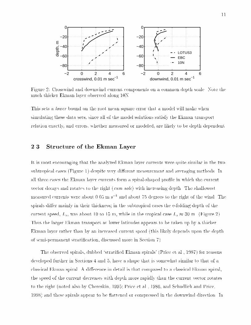
Figure 2: Crosswind and downwind current components on a common depth scale. Note themuch thicker Ekman layer observed along 10N.

This sets a lower bound on the root mean square error that a model will make when

simulating these data sets, since all of the model solutions satisfy the Ekman transport

relation exactly, and errors, whether measured or modeled, are likely to be depth-dependent.

2.3 Structure of the Ekman Layer

It is most encouraging that the analyzed Ekman layer currents were quite similar in the two

subtropical cases (Figure 1) despite very di�erent measurement and averaging methods. In

all three cases the Ekman layer currents form a spiral-shaped pro�le in which the current

vector decays and rotates to the right (cum sole) with increasing depth. The shallowest

measured currents were about 0.05 m s�1 and about 75 degrees to the right of the wind. The

spirals di�er mainly in their thickness; in the subtropical cases the e-folding depth of the

current speed, Ls, was about 10 to 15 m, while in the tropical case Ls � 30 m. (Figure 2).

Thus the larger Ekman transport at lower latitudes appears to be taken up by a thicker

Ekman layer rather than by an increased current speed (this likely depends upon the depth

of semi-permanent strati�cation, discussed more in Section 7).

The observed spirals, dubbed `strati�ed Ekman spirals' (Price et al., 1987) for reasons

developed further in Sections 4 and 5, have a shape that is somewhat similar to that of a

classical Ekman spiral. A di�erence in detail is that compared to a classical Ekman spiral,

the speed of the current decreases with depth more rapidly than the current vector rotates

to the right (noted also by Chereskin, 1995; Price et al., 1986, and Schudlich and Price,

1998) and these spirals appear to be attened or compressed in the downwind direction. In

12

e�ect, the direction and speed vary on di�erent depth scales, with the former being larger.

The shape of the spiral can be quanti�ed by a ' atness', Fl, the ratio of amplitude decay to

the turning rate,

Fl =@S

@z(S@�

@z)�1;

where S is the speed of the current. In a classical Ekman spiral (in�nite water depth,

Section 3.1) the speed decreases by one e-folding over a depth interval within which the

current turns through one radian and Fl = 1. The spirals of Figure 1 have an overall

atness, Fl = L�=Ls � 2 { 3, based upon the ratio of the turning depth to the e-folding

depth. When estimated by �nite di�erences over the discrete data, Fl � 2 averaged over the

upper half of the Ekman layer, and Fl � 3 over the lower half. An alternate and in some

ways more robust way to quantify the spiral shape is by the ratio of the standard deviations

of the crosswind and downwind current components,

Fv =rmsU 0

rmsV 0;

where this ()0 indicates the departure from the depth mean. Fv is also about 2 - 3 in these

cases.

The task for Ekman layer models can now be stated all too succinctly: to account for

the e-folding scale of the Ekman layer (i.e., the speed e-folding) as well as the at spiral

shape, or equivalently, the length scales for both speed and direction.

3 Di�usion Theories

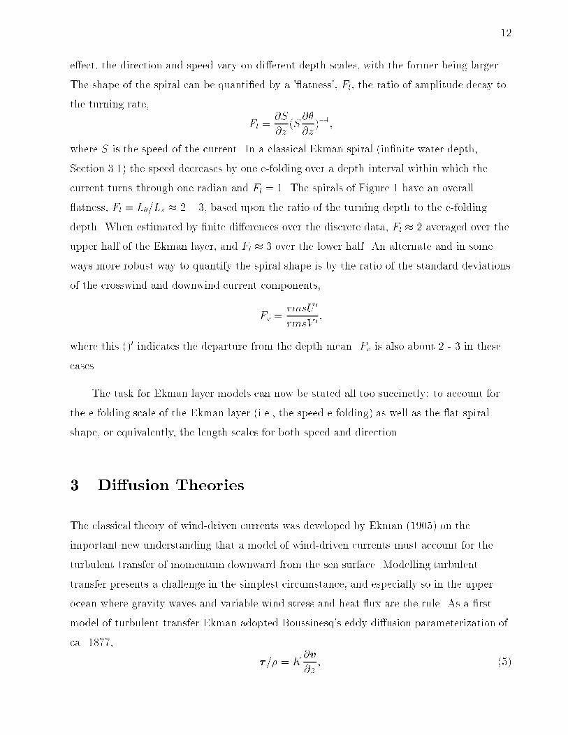
The classical theory of wind-driven currents was developed by Ekman (1905) on the

important new understanding that a model of wind-driven currents must account for the

turbulent transfer of momentum downward from the sea surface. Modelling turbulent

transfer presents a challenge in the simplest circumstance, and especially so in the upper

ocean where gravity waves and variable wind stress and heat ux are the rule. As a �rst

model of turbulent transfer Ekman adopted Boussinesq's eddy di�usion parameterization of

ca. 1877,

�=� = K@v

@z; (5)

13

where K is the eddy di�usivity (a concise and sympathetic review of the eddy di�usivity

parameterization is by Frisch, 1995; and see also Brown, 1991). A physical interpretation of

K is that it represents the stirring e�ects of turbulence; stirring the vertical shear of a

current produces a momentum ux down the local gradient. Similar turbulent transfer

parameterizations are widely used in ocean modelling, though are seldom the central issue,

as it is here.

The use of this parameterization shifts the Ekman layer problem onto the task of

�nding the appropriate K. Ekman (1905) knew from observations that the surface current

was the order of a few percent of the wind speed, which implies a boundary layer thickness

of a few tens of meters and K that is O(100� 10�4) m2 s�1. But he also suspected that K

would have a lively dependence upon external and internal parameters, wind speed and

strati�cation at the least. Considerable e�ort has gone toward estimating K from �eld

observations (Rossby and Montgomery, 1935; Neumann and Pierson, 1966; Pollard, 1975;

Huang, 1979; Schudlich and Price, 1998) though it is not evident that an accepted form of

the upper ocean K has emerged from this 'inductive diagnostic' program.

Our expectation is that there should exist a systematic stress/shear relationship, this

being di�erent only in detail from our assumption (Q4 of Section 1.1) that the current

pro�le holds a systematic relationship to the external variables. It remains to be seen

whether the upper ocean stress/shear relationship is consistent with a physical di�usivity,

i.e., a K that could be related to measurable, physical turbulence properties, or to a formal

di�usivity, i.e., any consistent relationship between stress and shear. To arrive at estimates

of K we will �rst compare the observations to simple solutions, much the way Ekman

suggested, and then estimate K using the steady momentum balance and the data alone. By

this roundabout path we hope to gain some insight into the di�culties encountered by the

inductive diagnostic program, and will �nally conclude that the fair weather, upper ocean K

is formal rather than physical.

3.1 The Laminar Di�usion Model

If the di�usivity is presumed to be steady but possibly dependent upon external variables

and depth, then from (3) and (5) the momentum balance for the time-averaged current is

14

just,

ifV =@

@zK@V

@z(6)

and the associated model is termed a `classical' di�usion model. Thus a classical model

attempts to calculate the mean current (and the mean stress) directly. If in addition K is

presumed to be constant with depth, then the model will be termed a classical `laminar'

di�usion model, or CLDM.2 The CLDM has as a solution the classical Ekman spiral, which

is a valuable reference or touchstone for boundary layer observations and theories (e.g.,

Stacey et al, 1986). The simple CLDM is unlikely to be the best possible di�usion model,

but before going on to more complex models it is useful to identify clearly what its

shortcomings may be.

In all of the solutions considered here the wind stress is taken to be steady and

northward (or imaginary) and the surface boundary condition at z = 0 is

K@V

@zjz=0 = i�w=�;

where �w is the given wind stress. The lower boundary condition is that the stress (and thus

the current shear) vanish at the given depth H,

@V

@zjz=�H = 0:

In Section 7 we will consider how time variations of H may a�ect the Ekman layer, but for

now H is taken to be the constant reference depth, zr, when simulating the three cases of

Section 2. More generally, H is identi�ed as the depth of semi-permanent strati�cation, i.e.,

the top of the seasonal or main thermocline (as mapped in Levitus, 1982, for example).

Subject to these boundary conditions the solution for the wind-driven current is

V = UH�r

1� s[exp(r �z0) + s exp(�r�z0)] (7)

over the depth range z0 = z=H > �1 and zero below. The scale

UH =U2

�

Hf

2Non-classical varieties have also been proposed. Section 4.2 considers brie y a model with depth- and

time-varying di�usivity. K could be ow-dependent and thus implicitly depth- and time-dependent as in

K-theory models, for example by Mellor and Durbin (1975), or the bulk boundary layer model of Large et al.,

1994. These latter models encompass the dynamics investigated in Sections 4 and 5. Non-classical di�usion

models generally have to be solved numerically and for that reason are not emphasized here.

15

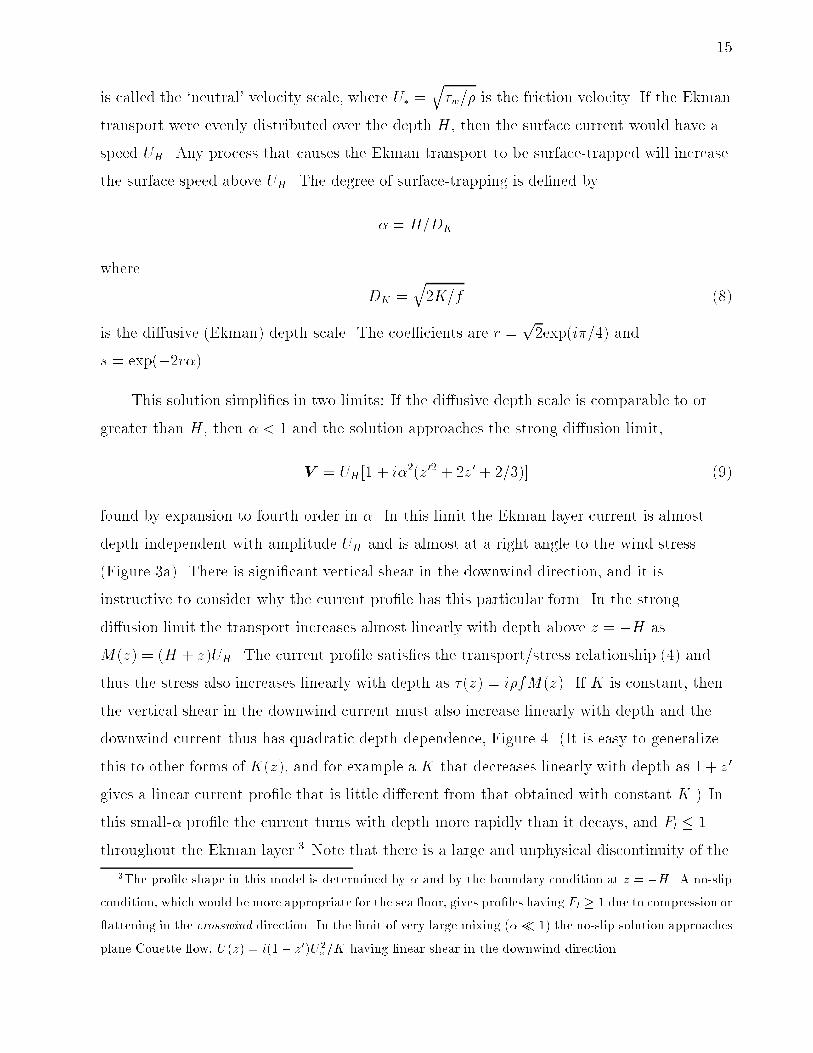
is called the `neutral' velocity scale, where U� =q�w=� is the friction velocity. If the Ekman

transport were evenly distributed over the depth H, then the surface current would have a

speed UH . Any process that causes the Ekman transport to be surface-trapped will increase

the surface speed above UH . The degree of surface-trapping is de�ned by

� = H=DK

where

DK =q2K=f (8)

is the di�usive (Ekman) depth scale. The coe�cients are r =p2exp(i�=4) and

s = exp(�2r�).

This solution simpli�es in two limits: If the di�usive depth scale is comparable to or

greater than H, then � < 1 and the solution approaches the strong di�usion limit,

V = UH [1 + i�2(z02 + 2z0 + 2=3)] (9)

found by expansion to fourth order in �. In this limit the Ekman layer current is almost

depth-independent with amplitude UH and is almost at a right angle to the wind stress

(Figure 3a). There is signi�cant vertical shear in the downwind direction, and it is

instructive to consider why the current pro�le has this particular form. In the strong

di�usion limit the transport increases almost linearly with depth above z = �H as

M(z) = (H + z)UH . The current pro�le satis�es the transport/stress relationship (4) and

thus the stress also increases linearly with depth as �(z) = i�fM(z). If K is constant, then

the vertical shear in the downwind current must also increase linearly with depth and the

downwind current thus has quadratic depth dependence, Figure 4. (It is easy to generalize

this to other forms of K(z), and for example a K that decreases linearly with depth as 1+ z0

gives a linear current pro�le that is little di�erent from that obtained with constant K.) In

this small-� pro�le the current turns with depth more rapidly than it decays, and Fl � 1

throughout the Ekman layer.3 Note that there is a large and unphysical discontinuity of the

3The pro�le shape in this model is determined by � and by the boundary condition at z = �H. A no-slip

condition, which would be more appropriate for the sea oor, gives pro�les having Fl � 1 due to compression or

attening in the crosswind direction. In the limit of very large mixing (�� 1) the no-slip solution approaches

plane Couette ow, U(z) = i(1� z0)U2

�=K having linear shear in the downwind direction.

16

02

4

02

4−1

−0.8

−0.6

−0.4

−0.2

0

U/UH

V/UH

CLDM

a

dept

h/H

02

4

02

4−1

−0.8

−0.6

−0.4

−0.2

0

U/UH

V/UH

CLDM

b

dept

h/H

02

4

02

4−1

−0.8

−0.6

−0.4

−0.2

0

U/UH

V/UH

SEL4

c

dept

h/H

02

4

02

4−1

−0.8

−0.6

−0.4

−0.2

0

U/UH

V/UH

SEL4

d

dept

h/H

02

4

02

4−1

−0.8

−0.6

−0.4

−0.2

0

U/UH

V/UH

CxLDM

e

dept

h/H

02

4

02

4−1

−0.8

−0.6

−0.4

−0.2

0

U/UH

V/UH

CxLDM

f

dept

h/H

Figure 3: Ekman layer current pro�les computed by three di�erent models for midlatitudeconditions, latitude = 37 degrees, �w = 0.08 Pa, and H = 50 m, which give a neutral velocityscale UH = 0:022 m s�1. a and b are from CLDM; c and d are from the four-layer strati�edEkman layer model, SEL4 developed in Section 5; e and f are from the complex laminardi�usion model, CXLDM, developed in Section 6. The CLDM solutions had K = 750 �10�4 and 50� 10�4 m2 s

�1, which correspond to � = 1:2 and 4:6 (a and b, respectively). The

SEL4 and CXLDM solutions had the same wind stress and Q = 100 and 1200 W m�2 (c andd, and e and f, respectively) so that � corresponds to the CLDM solutions at the top.

17

−0.5 0 0.5 1 1.5−1

−0.8

−0.6

−0.4

−0.2

0

current/UH

dept

h/H

downwind

crosswind

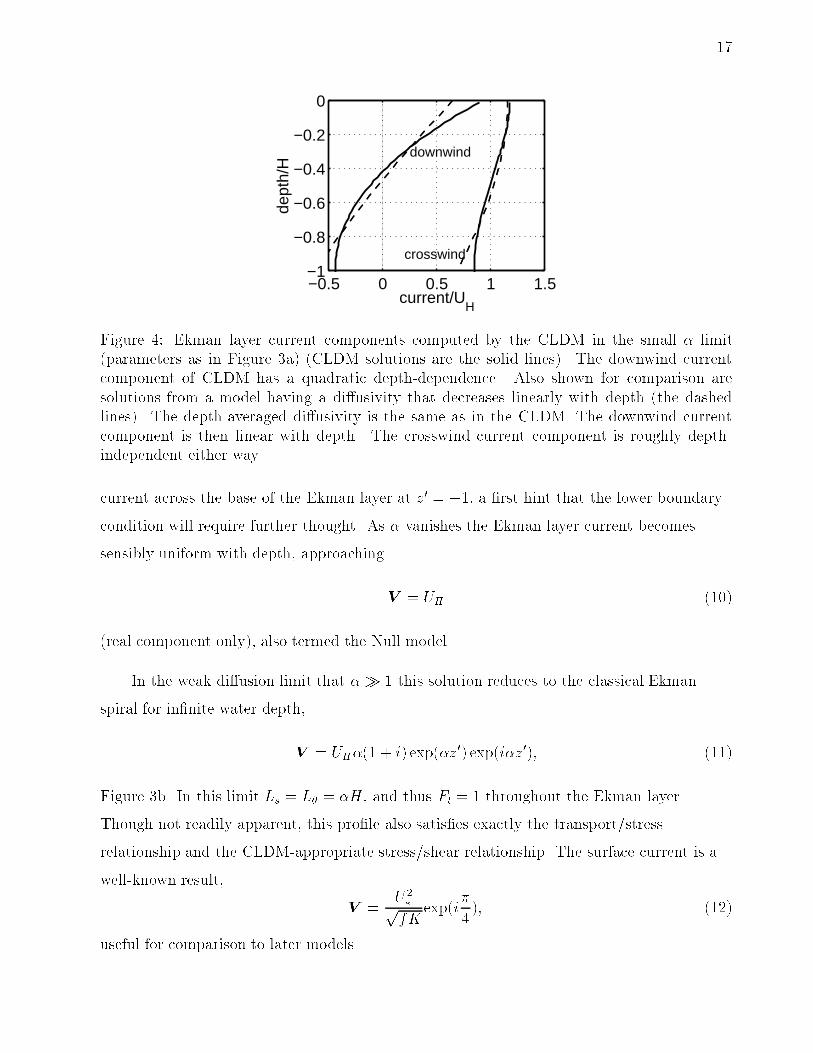
Figure 4: Ekman layer current components computed by the CLDM in the small � limit(parameters as in Figure 3a) (CLDM solutions are the solid lines). The downwind currentcomponent of CLDM has a quadratic depth-dependence. Also shown for comparison aresolutions from a model having a di�usivity that decreases linearly with depth (the dashedlines). The depth-averaged di�usivity is the same as in the CLDM. The downwind currentcomponent is then linear with depth. The crosswind current component is roughly depth-independent either way.

current across the base of the Ekman layer at z0 = �1, a �rst hint that the lower boundarycondition will require further thought. As � vanishes the Ekman layer current becomes

sensibly uniform with depth, approaching

V = UH (10)

(real component only), also termed the Null model.

In the weak di�usion limit that �� 1 this solution reduces to the classical Ekman

spiral for in�nite water depth,

V = UH�(1 + i) exp(�z0) exp(i�z0); (11)

Figure 3b. In this limit Ls = L� = �H, and thus Fl = 1 throughout the Ekman layer.

Though not readily apparent, this pro�le also satis�es exactly the transport/stress

relationship and the CLDM-appropriate stress/shear relationship. The surface current is a

well-known result,

V =U2

�pfK

exp(i�

4); (12)

useful for comparison to later models.

18

3.2 Evaluating the Classical, Laminar Di�usivity

The di�usivity has to be evaluated to complete the solution. Rather than sift through the

many forms that have been suggested (Huang, 1979), we set out to �nd the best-�t di�usion

coe�cient, Kb, that minimizes the mean square vector mis�t between the solution (7) and

the observed currents, � = 1

N�(V � V o)

2, case by case (Table 2) and where N is the number

of points observed. This is one implementation of the inductive diagnostic program referred

to above. Another method, suitable for the mid-latitude cases and leading to the same result,

would be to simply equate the depth scales Ls and L� with the di�usive depth scale DK .

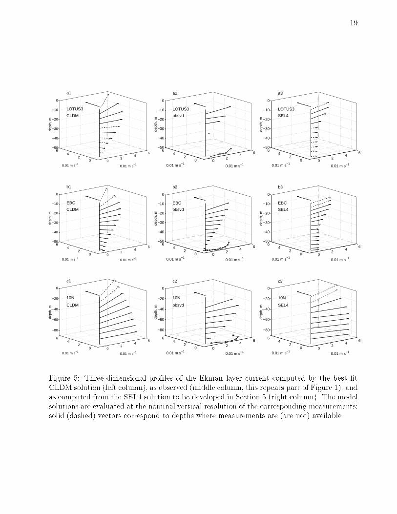
For the subtropical cases there was a distinct minimum of the mis�t and thus a

well-de�ned Kb and a CLDM solution that looks good (Figure 5a1,b1). In the EBC case the

CLDM solution has an rms mis�t of onlyp� = 0.007 m s�1, and the percent variance

accounted for, PV = 100(1� �= 1

N�V 2

o) = 89%. This rms mis�t is larger than but

comparable to the lower bound on the expected error estimated in Section 2.2

(� 0:004 m s�1.) Notice that the Null model accounts for a signi�cant fraction of the

variance. Since we are taking the Ekman transport relation for granted, it may be more

appropriate to compute the rms mis�t for the depth-dependent part of the current, in which

case the PV is considerably lower (the values in parentheses in Table 2).

The 10N case proved less amenable to this and to other models that will follow. The

mis�t did not have a sharp minimum value and the variance accounted by the optimum

solution was only 53% (or only 14% for the depth-dependent current). There are obvious,

large errors, especially in the lower half of the Ekman layer (Figure 5c1).4 About all that

can be said is that Kb appears to be larger than in the subtropical cases by a factor of about

two to three.

The variation of Kb and Ls between subtropics and tropics is very roughly proportional

to 1=f . This is reminiscent of the parameter dependence found in steady, neutral, turbulent

4The poor �t of the CLDM in the 10N case can be attributed in part to the transport discrepancy noted

in Section 2.2. If the wind stress is reduced by 30% to give a model-predicted transport consistent with the

observed transport, then the best �t solution (Kb = 400 m2 s�1) has much better statistics; the rms mis�t

is 0.015 m s�1 and PV = 83%. The current jump across z = �H is still unrealistic; this is likely to be a

shortcoming of the lower boundary condition and is not speci�c to the di�usion parameterization.

19

02

46

02

46

−50

−40

−30

−20

−10

0

0.01 m s−10.01 m s−1

CLDM

LOTUS3

a1

dept

h, m

02

46

02

46

−50

−40

−30

−20

−10

0

0.01 m s−10.01 m s−1

obsvd

LOTUS3

a2

dept

h, m

02

46

02

46

−50

−40

−30

−20

−10

0

0.01 m s−10.01 m s−1

SEL4

LOTUS3

a3

dept

h, m

02

46

02

46

−50

−40

−30

−20

−10

0

0.01 m s−10.01 m s−1

CLDM

EBC

b1

dept

h, m

02

46

02

46

−50

−40

−30

−20

−10

0

0.01 m s−10.01 m s−1

obsvd

EBC

b2

dept

h, m

02

46

02

46

−50

−40

−30

−20

−10

0

0.01 m s−10.01 m s−1

SEL4

EBC

b3

dept

h, m

02

46

02

46

−80

−60

−40

−20

0

0.01 m s−10.01 m s−1

CLDM

10N

c1

dept

h, m

02

46

02

46

−80

−60

−40

−20

0

0.01 m s−10.01 m s−1

obsvd

10N

c2

dept

h, m

02

46

02

46

−80

−60

−40

−20

0

0.01 m s−10.01 m s−1

SEL4

10N

c3

dept

h, m

Figure 5: Three-dimensional pro�les of the Ekman layer current computed by the best �tCLDM solution (left column), as observed (middle column, this repeats part of Figure 1), andas computed from the SEL4 solution to be developed in Section 5 (right column). The modelsolutions are evaluated at the nominal vertical resolution of the corresponding measurements;solid (dashed) vectors correspond to depths where measurements are (are not) available.

20

Ekman layers in which the only relevant time and velocity scales are f and U� (and

assuming that H is not important). That being the case, the thickness of the Ekman layer

should go as Ls = c1 U�=f where the similarity constant c1 = 0:25� 0:4 (Coleman et al.,

1990) and di�usivity K = c2 U2

�=f , where c2 � c21=2 = 0:03� 0:08. The estimated Ls and Kb

in these cases are consistent with this f;H-dependence, though with similarity 'constants'

(c1; c2) � (0:1; 0:01) that are roughly a factor of two to four lower than the nominal, neutral

values. Thus a 'parameterized' CLDM having K = c2U2

�=f and c2 = 0:01 gives a reasonable

simulation of these cases. A simpler, more concise model is di�cult to imagine.

There is trouble in the details, however. The reduced (compared to neutral) value of the

similarity constant c2 suggests that some process has caused these Ekman layers to be

somewhat surface-trapped (strati�cation is considered in Sections 4 and 5). It can expected

that c2 will take on other values in other circumstances, and so it isn't clear that this model

is useful for prediction. A close comparison of the modeled and observed spirals reveals what

appears to be a consistent error in the current direction. In the EBC case the modeled

currents are to the right of the observed currents by roughly 45 degrees in the lower half of

the Ekman layer (compare Figures 5b1 with 5b2). The directional error is reduced at

shallower depths, and hence is equivalent to an error in atness; the observations show

Fl � 2 near the surface and increasing somewhat with depth, while the CLDM spirals have a

atness Fl = 1 near the surface and decreasing slightly with depth. To be sure, the

directional or atness error made by the CLDM is small and near the uncertainty on the

observations. The atness error would not be considered signi�cant for most practical

purposes, but is signi�cant for Ekman layer models if, as we conclude below, it is evidence of

an irreducible error in the CLDM.

3.3 Nonlaminar and Nonclassical Di�usivities

In attempt to reduce the atness error we considered depth-dependent di�usivities. It is well

known that a K(z) which increases away from a no-slip boundary can reproduce a log layer

(Madsen, 1977), and we had expected to �nd something equivalent for the atness. Despite

a number of tries we did not discover a depth-dependent di�usivity that improved

appreciably on the laminar model; solutions continued to have excessively large downwind

21

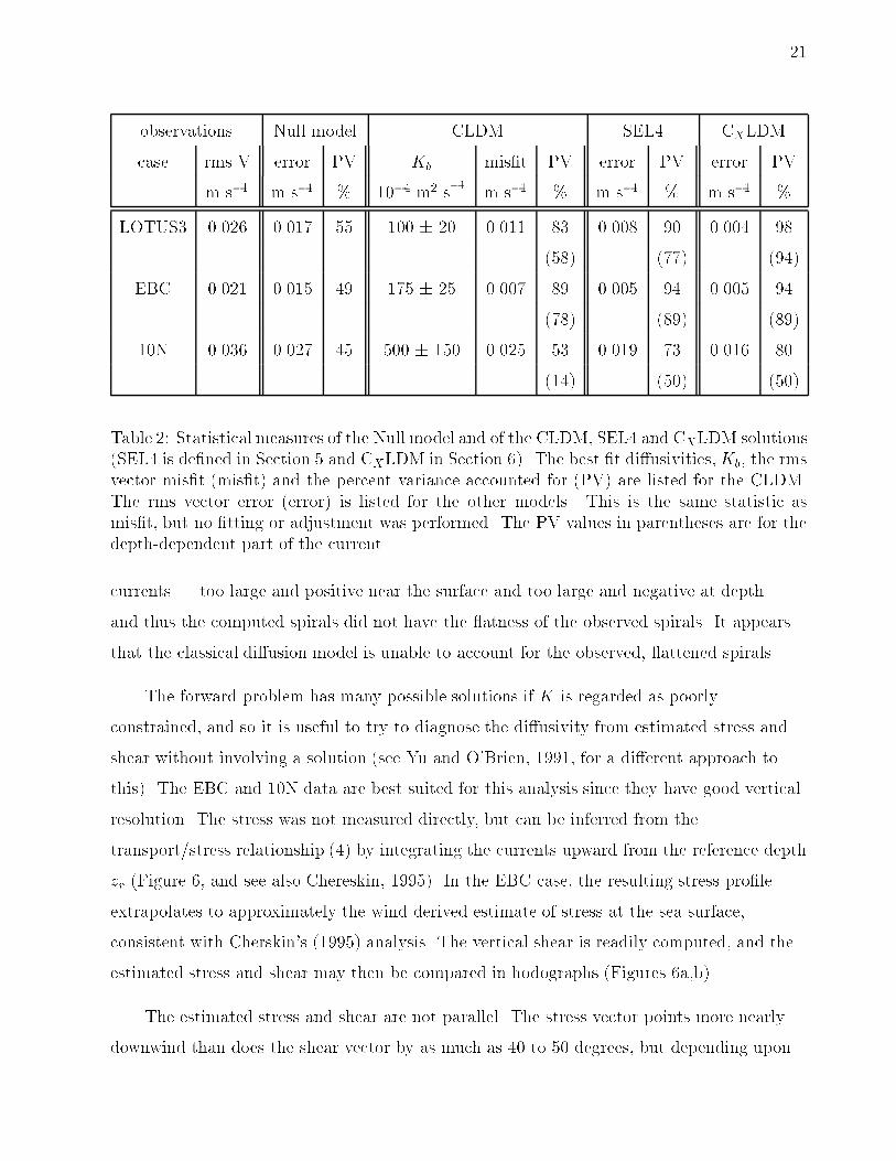
observations Null model CLDM SEL4 CXLDM

case rms V error PV Kb mis�t PV error PV error PV

m s�1 m s�1 % 10�4 m2 s�1

m s�1 % m s�1 % m s�1 %

LOTUS3 0.026 0.017 55 100 � 20 0.011 83 0.008 90 0.004 98

(58) (77) (94)

EBC 0.021 0.015 49 175 � 25 0.007 89 0.005 94 0.005 94

(78) (89) (89)

10N 0.036 0.027 45 500 � 150 0.025 53 0.019 73 0.016 80

(14) (50) (50)

Table 2: Statistical measures of the Null model and of the CLDM, SEL4 and CXLDM solutions(SEL4 is de�ned in Section 5 and CXLDM in Section 6). The best �t di�usivities,Kb, the rmsvector mis�t (mis�t) and the percent variance accounted for (PV) are listed for the CLDM.The rms vector error (error) is listed for the other models. This is the same statistic asmis�t, but no �tting or adjustment was performed. The PV values in parentheses are for thedepth-dependent part of the current.

currents | too large and positive near the surface and too large and negative at depth |

and thus the computed spirals did not have the atness of the observed spirals. It appears

that the classical di�usion model is unable to account for the observed, attened spirals.

The forward problem has many possible solutions if K is regarded as poorly

constrained, and so it is useful to try to diagnose the di�usivity from estimated stress and

shear without involving a solution (see Yu and O'Brien, 1991, for a di�erent approach to

this). The EBC and 10N data are best suited for this analysis since they have good vertical

resolution. The stress was not measured directly, but can be inferred from the

transport/stress relationship (4) by integrating the currents upward from the reference depth

zr (Figure 6, and see also Chereskin, 1995). In the EBC case, the resulting stress pro�le

extrapolates to approximately the wind-derived estimate of stress at the sea surface,

consistent with Cherskin's (1995) analysis. The vertical shear is readily computed, and the

estimated stress and shear may then be compared in hodographs (Figures 6a,b).

The estimated stress and shear are not parallel. The stress vector points more nearly

downwind than does the shear vector by as much as 40 to 50 degrees, but depending upon

22

−2 0 2 4 6−2

0

2

4

6

crossw stress, 0.01 Pa

dow

nw s

tres

s, 0

.01

Pa

b

423426

18

10

−1 0 1 2 3−1

0

1

2

3

crossw shear, 0.001 s−1

dow

nw s

hear

, 0.0

01 s

−1

a

42342618

10

0 0.02 0.04 0.06−80

−60

−40

−20

0

diffusivity mag, m2 s−1

dept

h, m

cEBC

10N

−20 0 20 40 60−80

−60

−40

−20

0

diffusivity angle, degde

pth,

m

d

Figure 6: Estimated stress, shear and di�usivity. (a) Vertical shear estimated from the EBCdata set and plotted in hodograph form. Depth in meters is at the tip of every second shearvector. (b) Stress inferred from the EBC data set using the steady momentum balance. (c)The magnitude of the complex di�usivity estimated from the EBC and 10N data sets (solidand dashed lines, respectively). (d) The rotation of the complex di�usivity, which shows theangle of the stress relative to the vertical shear. Angles greater than zero indicate that thestress vector is to the left of the corresponding shear vector, as can be seen comparing (a) and(b).

depth. This non-parallel stress/shear relationship is consistent with the atness of the

observed spirals [imagine a spiral with atness going to in�nity (no downwind current

component) in which case it is easy to see that the stress would have to be perpendicular to

the shear at every depth], and also with the di�culty we encountered when simulating the

observed current pro�les with the classical di�usion model. A non-parallel stress/shear

relationship has also been inferred from eddy-resolving numerical model solutions of

unsteady shear ows (Karniadakis and Brown, 1995), and of the planetary boundary layer

(Coleman et al., 1990), where it evidently results from the nonlocal character of turbulent

transfer, and also from surface drifter observations (Krauss, 1993). Whatever the source may

be, a non-parallel stress/shear relationship does not appear to be consistent with a physical

di�usivity, or at least not with the appealing notion of local eddy stirring of the mean shear.

23

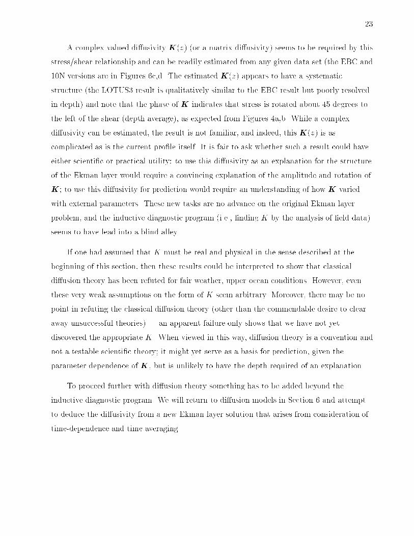
A complex-valued di�usivity K(z) (or a matrix di�usivity) seems to be required by this

stress/shear relationship and can be readily estimated from any given data set (the EBC and

10N versions are in Figures 6c,d. The estimatedK(z) appears to have a systematic

structure (the LOTUS3 result is qualitatively similar to the EBC result but poorly resolved

in depth) and note that the phase of K indicates that stress is rotated about 45 degrees to

the left of the shear (depth average), as expected from Figures 4a,b. While a complex

di�usivity can be estimated, the result is not familiar, and indeed, this K(z) is as

complicated as is the current pro�le itself. It is fair to ask whether such a result could have

either scienti�c or practical utility: to use this di�usivity as an explanation for the structure

of the Ekman layer would require a convincing explanation of the amplitude and rotation of

K; to use this di�usivity for prediction would require an understanding of how K varied

with external parameters. These new tasks are no advance on the original Ekman layer

problem, and the inductive diagnostic program (i.e., �nding K by the analysis of �eld data)

seems to have lead into a blind alley.

If one had assumed that K must be real and physical in the sense described at the

beginning of this section, then these results could be interpreted to show that classical

di�usion theory has been refuted for fair weather, upper ocean conditions. However, even

these very weak assumptions on the form of K seem arbitrary. Moreover, there may be no

point in refuting the classical di�usion theory (other than the commendable desire to clear

away unsuccessful theories) | an apparent failure only shows that we have not yet

discovered the appropriate K. When viewed in this way, di�usion theory is a convention and

not a testable scienti�c theory; it might yet serve as a basis for prediction, given the

parameter dependence of K, but is unlikely to have the depth required of an explanation.

To proceed further with di�usion theory something has to be added beyond the

inductive diagnostic program. We will return to di�usion models in Section 6 and attempt

to deduce the di�usivity from a new Ekman layer solution that arises from consideration of

time-dependence and time averaging.

24

4 The Process and Consequences of Diurnal Cycling

Under fair weather conditions the upper ocean is warmed by the sun and restrati�ed each

day (Price et al., 1986; Wij�els et al., 1994 and references therein). The diurnal cycle of

strati�cation is an important mode of variability in the upper 10 to 30 m of the water

column, and as Ekman (1905) anticipated, is likely to have a marked e�ect upon di�usivity

and thus upon wind-driven currents,

It is obvious that (the eddy di�usivity) cannot generally be regarded as a

constant when the density of the water is not uniform within the region

considered. For (the eddy di�usivity) will be greater within the layers of uniform

density and comparatively small within the transition-layers where the formation

of vortices must be much reduced owing to the di�erences in density.

The striking consequences of the covariation of strati�cation and di�usivity are evident in

the diurnal cycle of current observed under fair weather conditions in the subtropical North

Paci�c (Figure 7). During the evening and early morning the upper ocean was neutrally

strati�ed, i.e., was a density mixed layer, to a depth of about 20 { 30 m. There was

comparatively little vertical shear of the hourly-averaged current within this density mixed

layer (vertical shear remains measurable, O(10�3) s�1, and is generally in the downwind

direction). To a �rst approximation, velocity and density mixed layers were thus coincident.

As the surface layer was warmed by solar insolation during late morning, the wind stress

became trapped in a warmed surface layer that accelerated downwind and formed a

surface-trapped, half-jet dubbed the diurnal jet. The diurnal jet wass accelerated also by the

Coriolis force, which turned it to the right (northern hemisphere) in the sense of an inertial

motion. The jet grew in amplitude until about sundown, when the surface heat ux changed

to cooling. By that time the diurnal jet had turned roughly 90 degrees to the right of the

wind stress (along the 10N section the rotation would be only about a third of this). During

the evening and early morning the jet amplitude was rapidly reduced by vertical mixing

associated with the regrowth of the density mixed layer, and when the sun came up the

following day, the initial condition for the next diurnal cycle was a more or less 'clean slate'

(Stommel et al., 1969).

25

0 0.1 0.2 0.3 0.4 0.5 0.6 0.7 0.8 0.9 10

0.1

0.2

0.3

0.4

0.5

0.6

0.7

0.8

0.9

1

Fig 4 of PWP 1986 pasted in here

Figure 7: An observed diurnal cycle of temperature and current from Price et al., 1986.Currents were measured by VMCM current meters, smoothed over 30 min at a given depth,and referenced to 50 m depth. Temperature was measured by CTD and referenced to the seasurface. The uppermost dashed vector shows the wind stress direction.

26

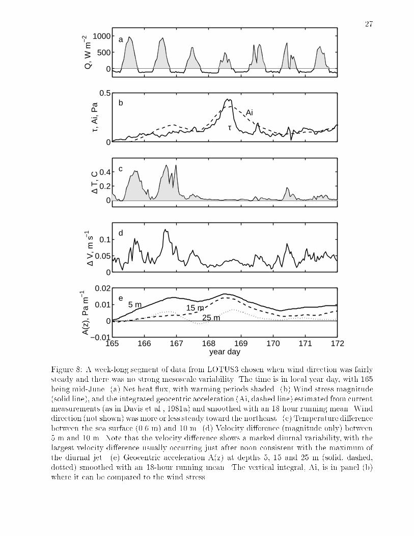
The thickness and amplitude of the diurnal jet varies with the surface heat ux and

wind stress, but the pattern described above repeats every day under fair weather conditions

(Figures 8, 9, 10). From these current and temperature observations we draw three

qualitative 'rules' useful for modelling the fair weather Ekman layer (relevant upper ocean

turbulence measurements are noted in brackets).

1) Most of the vertical shear of the wind-driven current occurs in conjunction with stable

strati�cation. Vertical shear within the density mixed layer is comparatively small (though

see Weller and Plueddemann, 1996). The latter implies that the eddy di�usivity within the

density mixed layer is large, O(1000� 10�4 m2 s�1), suggesting either intense or large

turbulent eddies. (Observations and highly resolved turbulence simulations indicate eddies

that sweep through the full thickness of the mixed layer (D'Asaro et al., 1996; D'Asaro and

Dairiki, 1997; Weller and Price, 1988; McWilliams et al., 1997).)

2) Turbulence and di�usivity within the strati�ed uid below the mixed layer are greatly

reduced compared with that in the mixed layer. (This is evident in observations of

temperature within the diurnal thermostad (Price et al., 1986) and in turbulent dissipation

measurements (Brainerd and Gregg, 1993a,b which show that it is not literally zero).)

3) Under fair weather conditions the thickness of the highly di�usive mixed layer goes

through a large amplitude diurnal cycle. (D'Asaro et al., 1996; D'Asaro and Dairiki, 1997;

Brainerd and Gregg, 1993a,b and references therein.)

4.1 A Depth and Time-Dependent Di�usion Model

The rules above can be implemented most simply within a depth- and time-dependent

di�usion model having a prescribed di�usivity. The di�usivity within a mixed layer of

thickness h(t) is made very large, K0 = 1000� 10�4 m2 s�1, as a �rst guess, and is assumed

to vanish below. The thickness of this mixed layer is made to go through a diurnal cycle

(sawtooth form) having a daytime minimum at the sea surface (to avoid introducing a

parameter) and a nighttime maximum of 50 m, thus causing a depth- and time-dependent K,

K(z; t) = K0 if 0 > z > �h(t); and

= 0 otherwise:

27

0

500

1000

Q, W

m−

2 a

0

0.5τ,

Ai,

Pa b

τ

Ai

0

0.2

0.4

∆ T

, C

c

0

0.05

0.1

∆ V

, m s

−1 d

165 166 167 168 169 170 171 172−0.01

0

0.01

0.02

year day

A(z

), P

a m

−1

e5 m 15 m

25 m

Figure 8: A week-long segment of data from LOTUS3 chosen when wind direction was fairlysteady and there was no strong mesoscale variability. The time is in local year day, with 165being mid-June. (a) Net heat ux, with warming periods shaded. (b) Wind stress magnitude(solid line), and the integrated geocentric acceleration (Ai, dashed line) estimated from currentmeasurements (as in Davis et al., 1981a) and smoothed with an 18-hour running mean. Winddirection (not shown) was more or less steady toward the northeast. (c) Temperature di�erencebetween the sea surface (0.6 m) and 10 m. (d) Velocity di�erence (magnitude only) between5 m and 10 m. Note that the velocity di�erence shows a marked diurnal variability, with thelargest velocity di�erence usually occurring just after noon consistent with the maximum ofthe diurnal jet. (e) Geocentric acceleration A(z) at depths 5, 15 and 25 m (solid, dashed,dotted) smoothed with an 18-hour running mean. The vertical integral, Ai, is in panel (b)where it can be compared to the wind stress.

28

−0.4 −0.2 0 0.2 0.4−0.4

−0.2

0

0.2

0.45 m

dow

nwin

d, m

s−

1

−0.4 −0.2 0 0.2 0.4−0.4

−0.2

0

0.2

0.415

dow

nwin

d, m

s−

1

−0.4 −0.2 0 0.2 0.4−0.4

−0.2

0

0.2

0.425

dow

nwin

d, m

s−

1

−0.4 −0.2 0 0.2 0.4−0.4

−0.2

0

0.2

0.435

crosswind, m s−1

dow

nwin

d, m

s−

1

−0.1 0 0.1 0.2 0.3−0.2

−0.1

0

0.1

0.2

1

4

710 13

16

1922

5 m

−0.1 0 0.1 0.2 0.3−0.2

−0.1

0

0.1

0.2

1

4

710

13

16

1922

15

−0.1 0 0.1 0.2 0.3−0.2

−0.1

0

0.1

0.2

14

710

13

16

1922

25

−0.1 0 0.1 0.2 0.3−0.2

−0.1

0

0.1

0.235

crosswind, m s−1

Figure 9: Current hodographs from a week-long segment of LOTUS3 data. Left column:Hourly averaged current (dots) at 5, 15, 25 and 35 m depth and the time-averaged current(the small central vector) are shown in a downwind and crosswind coordinate system. Rightcolumn: Ensemble, diurnal-averaged currents (note the scale change compared to the leftcolumn). The roughly circular array of dots denote the velocity vector at hourly intervals,every third of which is labeled (local time). Thus the diurnal maximum at 5 m depth occurs atca. 16L when the current is owing about 90 degrees to the right of the wind stress. The smallcentral vectors show the time-averaged current. Note that the time-averaged current at 5 mdepth is about half the magnitude of the diurnal cycle, while at 25 m depth the time-averagedcurrent is much smaller than the diurnal cycle, the latter being a near-inertial oscillation.

29

166

168

170

172 −50

−40

−30

−20

−10

0

−3

−2

−1

0

depth, m

time, days

aT

emp,

C

165 166 167 168 169 170 171 172−50

−45

−40

−35

−30

−25

−20

−15

−10

−5

0

year day

dept

h, m

∆ T = 0.03 C

0.3 C

1 C

b

Figure 10: Temperature measured by vector-measuring current meters referenced to the sur-face in order to show the changing depth of strati�cation during the week-long period shownin the previous two �gures. (a) Temperature displayed as a contoured surface. (b) Depthwhere the temperature changed (decreased) from the surface value by 0.03 C (dotted line),0.3 C (dashed line), and 1 C (solid line). These time series have rather coarse depth resolutionset by the depths of the current meters.

The momentum equation is the time-dependent form (2), and surface and lower boundary

conditions are as before. This model is readily solved numerically and the time-averaged

current pro�le computed from the solution. The thing of interest is whether the solution

spiral has a more realistic, attened shape than did solutions of the classical di�usion model.

Indeed, it does (Figure 11), and the amplitude is realistic as well. An important result of

sensitivity experiments is that solutions of this model are almost independent of Ko provided

that it is at least as large as the value 1000� 10�4 m2 s�1 used here. This is a remarkable

simpli�cation over the classical di�usion models in that a realistic solution emerges from

implementing three, largely qualitative rules.

To appreciate some of the consequences of a time- and depth-varying K it is helpful to

examine a Reynolds decomposition of the mean stress,

� = K@v

@z= K 0

@v0

@z+K

@V

@z;

and where v = V + v0, as before. The mean term (second term on rhs) is analogous to the

classical di�usion parameterization (7) in that it is proportional to the shear of the mean

current. The eddy term (�rst term on the rhs) is as large as the mean term and is not

30

−1 0 1 2 3 4 5 6−3

−2

−1

0

1

2

3

4

crosswind current, 0.01 m s−1

dow

nwin

d cu

rren

t, 0.

01 m

s−

1

8

1624

3240

τ

a

−5 0 5 10−50

−40

−30

−20

−10

0

crosswind, 0.01 m s−1

dept

h, m

b

−5 0 5 10−50

−40

−30

−20

−10

0

downwind, 0.01 m s−1

Figure 11: Solutions of the depth- and time-dependent di�usion model. External pa-rameters were set to those of the EBC case, and the mixed layer di�usivity was K0 =1000 � 10�4 m2 s�1. (a) A solution hodograph that can be compared to Figure 1c. (b)(b) Crosswind and downwind currents that can be compared with EBC data shown as thediscrete points.

−0.2 0 0.2−50

−45

−40

−35

−30

−25

−20

−15

−10

−5

0

dept

h, m

crosswind stress, Pa

eddy

mean

sum

−0.2 0 0.2−50

−45

−40

−35

−30

−25

−20

−15

−10

−5

0

downwind stress, Pa

eddy

mean

sum

Figure 12: Stress pro�les (solid lines) and their Reynolds decomposition into mean (dashed)and eddy (dotted) components computed from the solutions of the depth- and time-dependentdi�usion model. Note that the eddy component is as large as the mean component, and thatthe eddy and mean terms almost cancel in the crosswind direction. If they had canceledcompletely the current spiral would be entirely attened in the downwind direction.

31

parallel to it or to the mean stress (Figure 12). Thus it is evident that an accurate

parameterization of the mean stress given only the mean current will require a complex

di�usivity having a signi�cant rotation (small near the surface and increasingly positive at

depth, averaging about �/4). This is consistent with the di�usivity from observations in

Section 3.3, and as we have implied before, consistent also with the attened shape of the

fair weather spiral.

5 A Layered Model of Diurnal Cycling

The previous results suggests that one way to arrive at a physically-based model of the fair

weather Ekman layer might be to solve for the time-average of an upper ocean that is

subject to diurnal cycling. The full problem has mixed time and space dependence, and

probably requires numerical solution as above. However, the observations and results above

suggest further simpli�cations that will lead to a simple, explicit solution.

5.1 Model Formulation and Integration

As an approximation one could assume that the di�usivity within the density mixed layer is

e�ectively in�nite, i.e., that the density mixed layer is also a velocity mixed layer. Going

further and taking the lower interface of the mixed layer to be steplike gives a two-layer form

of the momentum equations in which wind stress is absorbed entirely within a density mixed

layer of time-varying thickness h(t),

@v

@t+ ifv = �We

�v

h+

1

�h� : (13)

The entrainment velocityWe =@h@t

when � 0, and vanishes otherwise. The velocity di�erence

�v is taken across the base of the mixed layer. The uid below the mixed layer is unforced,

@v

@t+ ifv = 0; (14)

which holds down to z = �H, the deepest extent of the mixed layer and Ekman layer.

A crucial part of the problem is to specify the strati�cation represented by the depth of

semi-permanent strati�cation, H, and the time-varying mixed-layer depth, h(t). H is

32

presumed to be the top of the seasonal or main thermocline and is thus set by processes that

may be inherently nonlocal, as for example the east{west tilt of the tropical Paci�c

thermocline (Wij�els, et al., 1994). For now, H is taken to be given and steady so that we

can emphasize the e�ect of time-varying h(t) (variable H will be considered in Section 7 and

shown to be important, especially in the tropics). In fair weather conditions the variation of

mixed layer depth h(t) will be associated primarily with the diurnal cycle. To model the

consequences of this variation we make the simplifying assumption that h varies with a

top-hat time-dependence over the course of a day, though the actual time dependence is

smoothly varying, especially evident in the afternoon deepening phase (Figure 7). The

nighttime mixed layer depth is taken to be the given depth of semi-permanent strati�cation,

hnight = H;

while the shallower, daytime mixed layer depth is taken to be the so-called trapping depth of

Price et al. (1986),

hday = DQ =U2

�P�q

Q�PQ=2:; (15)

where P� = (1=f)q2� 2cos(fPQ=2), Q� = g�Q=(�Cp) [l2 t�3], with g the acceleration of

gravity, � the thermal expansion coe�cient, and Cp the heat capacity of sea water (constant

for a given case), Q is the daily maximum surface heat ux, and PQ is the period over which

the net surface heat ux is warming. We are assuming an idealized surface heat ux that

oscillates diurnally with zero long term mean to produce closed diurnal cycles. Q is thus a

measure of the variability of the surface heat ux, which is extremely important because

heat and cooling have quite distinct and asymmetric e�ects upon the upper ocean. If the

diurnal cycles are closed and repeating, then the interval PQ used by Price et al. (1986) can

be approximated by half a day, PQ � ��1, where = 2� day�1, and for this purpose

� (4�=f)sin(�) where � is the latitude. The depth DQ is termed the diurnal warm layer

depth or thickness, and derives from a bulk Richardson number condition upon the shear

and strati�cation of the diurnal warm layer. (That hday should be strictly equal to DQ is not

obvious a priori as noted below.) This DQ is analogous to the di�usive depth, DK , of the

classical di�usion model (Section 3.2), but note that DQ depends only upon external

variables. It can be evaluated for the three cases considered here, and DQ = 13, 17 and 25 m

for LOTUS3, EBC and 10N, respectively. This can be compared to the observed e-folding

33

depth of the current speed, 10, 16 and 32 m, (Table 1), though the analogy is not complete

(more on this in Section 5.5).

Given that the strati�cation is speci�ed, the remaining task is to integrate the

momentum equations, and then time-average the solution (rather than time-average the

momentum equation). This can be greatly simpli�ed by noting that vertical shear will occur

only when the diurnal strati�cation is `on', i.e., when h = DQ. Otherwise, the current pro�le

is vertically homogeneous above z = �H. The initial condition for the diurnal jet is thus a

vertically uniform current pro�le. The vertical shear of the subsequent wind-driven current

is then independent of the initial condition and the shear follows the Fredholm solution for

the impulsive start-up of a layer of thickness h = DQ, forced by a wind stress switched on at

t = 0,

�v =U2

�

fDQ

[1� exp (�ift)] = UQ : (16)

This holds for half a day, t = ��1, after which the shear vanishes along with the diurnal

warm layer. The scale

UQ =U2

�

fDQ

=

qQ���1=2

fP�(17)

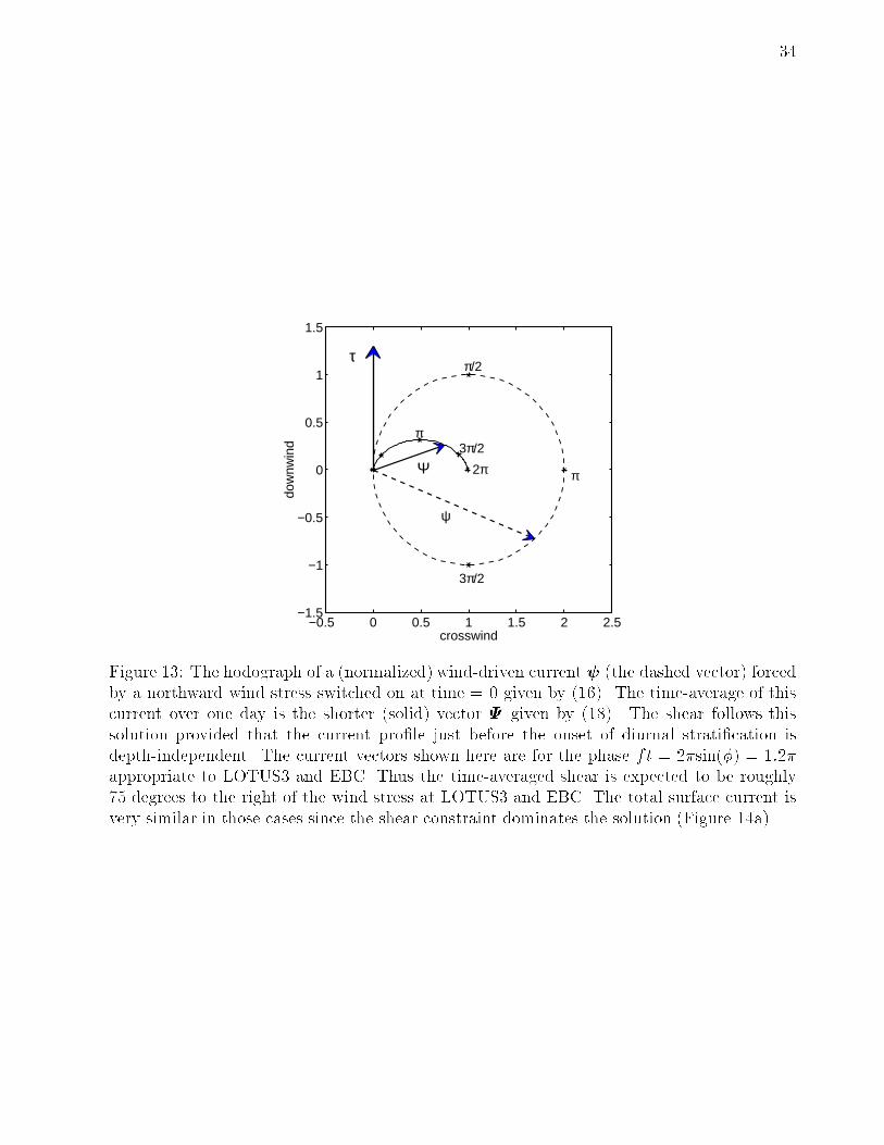
is the amplitude of the diurnal jet and is plotted in Figure 13b. So far as the vertical

shear is concerned, each day is the same as the last and thus the time-averaged shear is

equal to the shear averaged over just one day,

�V =UQ

2��1

Z ��1

0

dt = UQ : (18)

The time-averaged is

=1

2+

i

4�sin(�)[1� exp(�i2�sin(�))]; (19)

a function of latitude alone, and also plotted in Figure 13b. Eq (18) will be referred to as

the shear constraint. A second integral comes from noting that the time averaged transport

above z = �H must be the Ekman transport regardless of strati�cation and diurnal cycling

and thus,

V1DQ + V2(H �DQ) =U2

�

f; (20)

which will be referred to as the transport constraint. V1 is the current above z = �DQ and

V2 is the current from �H < z < �DQ. The time-averaged current follows immediately,

V (z0) = UH [1 + (�c(z0)� 1) ] ; (21)

34

−0.5 0 0.5 1 1.5 2 2.5−1.5

−1

−0.5

0

0.5

1

1.5

τπ/2

π

3π/2

π3π/2

2πΨ

ψ

crosswind

dow

nwin

d

Figure 13: The hodograph of a (normalized) wind-driven current (the dashed vector) forcedby a northward wind stress switched on at time = 0 given by (16). The time-average of thiscurrent over one day is the shorter (solid) vector given by (18). The shear follows thissolution provided that the current pro�le just before the onset of diurnal strati�cation isdepth-independent. The current vectors shown here are for the phase ft = 2�sin(�) = 1:2�appropriate to LOTUS3 and EBC. Thus the time-averaged shear is expected to be roughly75 degrees to the right of the wind stress at LOTUS3 and EBC. The total surface current isvery similar in those cases since the shear constraint dominates the solution (Figure 14a).

35

−0.02 0 0.02 0.04 0.06 0.08−0.04

−0.02

0

0.02

0.04

0.06

acrosswind, m s−1

dow

nwin

d, m

s−

1

V1

V2

UH

δ V

a LOTUS3 and EBC

−0.02 0 0.02 0.04 0.06 0.08−0.04

−0.02

0

0.02

0.04

0.06

acrosswind, m s−1

dow

nwin

d, m

s−

1 V1

V2

UH

δ V

b 10N

Figure 14: Solutions of SEL2 for external parameters of (a) LOTUS3 (very nearly EBC), and(b) 10N. The wind stress (not shown) is due 'north'.

where UH = U2

�=fH as in the CLDM solution, and where

� = H=DQ =HqQ���1=2

U2�P�

;

which is analogous to the ratio H=DK of the CLDM. The depth z0 = z=H, and c is a ag

that turns on or o� depending upon depth; c = 1 if �z0 > �1 (within the diurnal warm

layer, layer 1), and c = 0 if �z0 < �1 (below the diurnal warm layer, layer 2). This solution

depends only upon external parameters and can be evaluated readily (Figure 14).

For some purposes, e.g., examining the parameter dependence of the surface current,

this two-layered, strati�ed Ekman layer solution, termed SEL2, could be considered

complete. However, for most practical purposes it is useful or even necessary to make the

solution at least semi-continuous with depth. This can be done in two di�erent ways; by

de�ning the equivalent di�usion parameterization (taken up in Section 6), or by the addition

of layers.

5.2 Some Additions and a Check

The two layer model taken literally indicates a velocity jump between the layers. There is, of

course, no such velocity jump found in the ocean, nor in any highly resolved upper ocean

model. To represent the interface between these layers, a third layer of thickness DQ is

36

inserted between layers one and two, and the current in this intermediate layer is computed

by a linear interpolation in the depth range 1

2DQ < �z < 3

2DQ. Another velocity jump

occurs at the bottom of the Ekman layer, z = �H. At subtropical or higher latitudes this

velocity jump will usually be quite small. However at lower latitudes the deep Ekman layer

currents can be fairly large, O(0.1 m s�1), and cause signi�cant mixing. To simulate this

feature, a fourth (and �nal) layer is added to the bottom of the Ekman layer. The thickness

of layer four is set by a critical gradient Richardson number condition (but as we will discuss

shortly the lower interface layer evident in the observations is much thicker than this yields).

The embellished, semi-continuous solution has four distinct layers, two uniform and two

sheared, and is termed SEL4 (four-layer strati�ed Ekman layer).

The dynamics represented by SEL4 are a subset of the dynamics in the Price et al.

(1986) upper ocean numerical model (PWP), and SEL4 could be regarded as an

approximate solution for idealized surface uxes. To check the approximations made during

the derivation of SEL4 it is useful to compare SEL4 with time-averaged solutions computed

from the PWP numerical model, Figure 15. From this it would appear that SEL4 is a

faithful rendition of the PWP physics, which is all that could have been expected.5

5.3 Comparison With the Observations

Given the surface uxes of momentum and heat, and assuming that the depth of

semi-permanent strati�cation is known from climatology or direct observation, then the

SEL4 solution can be evaluated unambiguously and compared directly with observations

5It is notable that SEL2 is an Ekman layer solution free of tunable parameters and similarity constants

(though the addition of layers three and four to make SEL4 represented a gross and ad hoc adjustment

of the pro�le structure). This must be fortuitous because there was no way to assert a priori two of the

approximations used in the derivation. Speci�cally, the trapping depth was expected to be proportional to

the thickness of the diurnal warm layer, but not necessarily equal to it, and in the same way the top-hat time

dependence assumed for the diurnal variation of the mixed layer depth can only be approximate. During the

initial development of the SEL2 solution it was presumed that the time during which h = hday should be set

equal to ��1, with expected to be roughly 1, but made available as an adjustable parameter. Subsequent

comparison of SEL2 and SEL4 with PWP numerical solutions showed that the optimum choice, = 1.1, gave

only a very slightly enhanced �t to the numerical solutions, and hence was omitted. The SEL2 solution is

approximate for other reasons, including that optical properties are ignored.

37

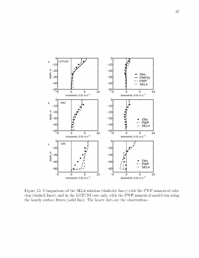
−5 0 5 10−50

−40

−30

−20

−10

0LOTUS3

crosswind, 0.01 m s−1

dept

h, m

−5 0 5 10−50

−40

−30

−20

−10

0

downwind, 0.01 m s−1

a

ObsPWP(t)PWPSEL4

−5 0 5 10−50

−40

−30

−20

−10

0EBC

crosswind, 0.01 m s−1

dept

h, m

−5 0 5 10−50

−40

−30

−20

−10

0

downwind, 0.01 m s−1

b

ObsPWPSEL4

−5 0 5 10

−80

−60

−40

−20

0

crosswind, 0.01 m s−1

10N

dept

h, m

−5 0 5 10

−80

−60

−40

−20

0

downwind, 0.01 m s−1

c

ObsPWPSEL4

Figure 15: Comparisons of the SEL4 solution (dash-dot lines) with the PWP numerical solu-tion (dashed lines), and in the LOTUS3 case only, with the PWP numerical model run usingthe hourly surface uxes (solid line). The heavy dots are the observations.

38

(Figure 5). In the subtropical cases the agreement appears to be fairly good visually, and

notice in particular that these solutions have a attened spiral shape, Fv � 2:5, that proved

di�cult for the classical di�usion model. For the LOTUS3 case the rms vector error is

0.008 m s�1 and the percent variance accounted for by the SEL4 solution is PV = 90%. For

the EBC case the rms vector error is 0.005 m s�1, and PV is a little more than 90%. These

are slightly better than the optimum CLDM solution (Table 2).

The SEL4 solution is less successful in the 10N case: The rms vector error is 0.019

m s�1, and PV is only 73% (still a little better than the optimum CLDM solution). Almost

all of the error comes from depths of 50{70 m, where the SEL4 solution overestimates the

crosswind currents. An error of that sense is bound to occur somewhere in the water column

since the predicted Ekman transport exceeds the measured transport by some 30%.6 Even

with allowance for the transport discrepancy in the 10N data set it remains that the shear

across the base of the Ekman layer is much too abrupt (the same error is evident in the

CLDM solutions (Figure 5) and is likely due to the lower boundary condition, Section 7).

5.4 Parameter Dependence of SEL2

Before discussing parameter dependence in detail it is helpful to consider what SEL2 (or 4)

have added to the list of relevent external variables. The absolute minimum set of relevent

external variables that would appear in a model of the Ekman layer current, U , would surely

include z; U�; f and H. A non-dimensional solution could then be written in the form

U

UH

= function(z0; �)

where z0 = zHand � = H

DKwith D =

q2Kf

or / U�f, the latter corresponding to the

parameterized CLDM solution. Explicit treatment of the diurnal cycle and time-averaging

introduced two new external variables, Q� and �1, and the solution would then be

U

UH

= function(z0; �; f=)

6If the wind stress is reduced by 30% so that the predicted transport matches the observed transport, then

the rms mis�t of SEL4 is 0:009 m s�1 and PV = 94%. Recall the similar improvement in the statistical �t of

the CLDM solution, Section 3.2

39

where z0 and � = HDQ

have much the same roles as in the di�usion theories, while

f= / sin(�) is new. This additional, separate dependence upon latitude sets the SEL2

solution apart from classical di�usion theories, and admits attened (or not) spirals.

5.4.1 Heating and Wind Stress

Heating and wind stress a�ect the structure of the SEL2-predicted Ekman layer in a

straightforward way that follows from the �-dependence noted above. It is evident from (21)

that when � = H=DQ ! 1 the e�ects of diurnal cycling will be negligible. In that limit the

surface current and the deep current (layers one and two) both go to the Null model

V = UH ; (22)

as in the vanishing � limit of the CLDM, (10) and Figures 3a,c. This is an important limit

about which this model has nothing interesting to say (see instead Gnanadesikan and

Weller, 1995 and McWilliams et al., 1997).

The SEL2 solution is relevant in the limit, � � 1, or in terms of external parameters,

pQ���1H

U2�P�

� 1; (23)

which de�nes 'fair weather' for our purpose. In this limit the e�ect of diurnal cycling on the

Ekman layer structure may be substantial, but to tell for sure the upper layer current has to

be compared to the neutral velocity scale UH and this depends upon both � and the latitude

through the phase (the amplitude of which is in Figure 16c). Outside of the tropics,

� � 30 deg, and assuming that �� 1 then the layer one current is determined by the shear

constraint alone,

V1 � UQ =

qQ���1=2

fP� ; (24)

and the speed is independent of the wind stress (the warm layer thickness is proportional to

the wind stress and thus the speed of the diurnal jet is independent of the wind stress, Price

et al., 1986). The subtropical cases are close to this limit, as can be seen in in Figure 14a.

The speed computed from (24) is � 0:04 m s�1 and the direction of is about 75 degrees to

the right of the wind stress (Figure 13), both of which are consistent with the shallowest

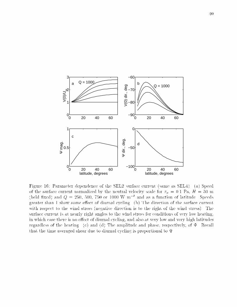
40

0 20 40 60−90

−80

−70

−60

V(0

) di

r., d

eg Q = 1000b

0 20 40 600

1

2

3

V(0

)/U

H

Q = 1000a

0 20 40 600

0.5

1

Ψ m

ag.

c

latitude, degrees0 20 40 60

−100

−50

0Ψ

dir.

, deg

.

latitude, degrees

d

Figure 16: Parameter dependence of the SEL2 surface current (same as SEL4). (a) Speedof the surface current normalized by the neutral velocity scale for �w = 0.1 Pa, H = 50 m(held �xed) and Q = 250, 500, 750 or 1000 W m�2 and as a function of latitude. Speedsgreater than 1 show some e�ect of diurnal cycling. (b) The direction of the surface currentwith respect to the wind stress (negative direction is to the right of the wind stress). Thesurface current is at nearly right angles to the wind stress for conditions of very low heating,in which case there is no e�ect of diurnal cycling, and also at very low and very high latitudesregardless of the heating. (c) and (d) The amplitude and phase, respectively, of . Recallthat the time-averaged shear due to diurnal cycling is proportional to .

41

observed currents at LOTUS3 or EBC (Figures 1a,c). Thus the SEL2 solution gives a

slightly surprising explanation of a fairly ordinary fact.

Aside from the near-equatorial region, most days and most places will fall between the

neutral and fair weather extremes noted above and the SEL2 surface current will depend

upon both H and DQ. The stress-dependence of the surface current will then be

intermediate as well.

The sensitivity to errors in the surface uxes can be evaluated by calculating perturbed

solutions in which � and Q are varied by a nominal uncertainty, 20%, and then computing

the PV between the nominal and perturbed solutions. For mid-latitude conditions, �

uncertainty of 20% gives PV = 95 (88)%, where the value in parentheses is for the

depth-dependent part. For 10N conditions, PV = 96 (68)%, or comparable to the errors

found in the best models. The sensitivity to the heat ux is much less, PV = 99 (97)% for

mid- or tropical latitudes. Errors in the estimated heat ux are probably not a major

contributor to error in the simulations, while error in wind stress clearly could be, especially

in the tropics.

In any �eld data set the meteorological conditions are bound to vary from day to day,

so that the surface uxes must also vary from day to day. It has been assumed implicitly

that the surface uxes could be represented by their averaged values, i.e., the time-averaged

wind stress and the average of the daily maximum heat ux. However, the SEL4 solution is

not linear in these variables, and hence the use of averaged uxes must induce an error in

the simulations of �eld data. To get a sense of the magnitude we have computed the average

current over an ensemble of solutions in which � was varied from 0.05 to 0.25 Pa while Q

was simultaneously varied from 300 to 800 W m�2, and compare this ensemble average

solution (which could always be computed if the surface uxes were known in detail) to the

single solution computed from the averages of � and Q (Figure 17a). The error induced by

the use of the averaged surface uxes appears to be small compared to the typical current

(less than 10% over most of the Ekman layer) and within the uncertainty associated with

current sampling or stress estimation. Interestingly, the use of an averaged H may lead to

somewhat larger errors (Section 7).

42

−0.02 0 0.02 0.04 0.06−60

−50

−40

−30

−20

−10

0

dept

h, m

crosswind, m s−1

aaaaaaaaaaaaaaaaaaaaaaaaaaaaaaaaaaaaaaaaaaaaaaaaaaaaaaaaaaaaaaaaaaaaaaaaaaaaaaaaaaaaaaaaaaaaaaaaaaaaaaaaaaaaaaaaaaaaaaaaa

−0.02 0 0.02 0.04 0.06−60

−50

−40

−30

−20

−10

0

downwind, m s−1

0 0.05 0.1−100

−80

−60

−40

−20

0

dept

h, m

crosswind, m s−1

b

0 0.05 0.1−100

−80

−60

−40

−20

0

downwind, m s−1

Figure 17: Ensemble-averaged solutions of SEL4. (a) Crosswind and downwind current com-ponents computed from SEL4 for mid-latitude conditions (f and H of LOTUS3) with varying�w over the range 0.025 to 0.25 Pa and Q over the range 300 to 800 W m�2. The thin dottedlines are the individual solutions; the heavy solid line is the ensemble average of these solu-tions, and the heavy dashed line is the solution for the average � and Q. These two averagedcurrent pro�les are fairly similar in this example, suggesting that the use of averaged surface uxes induces acceptable errors. (b) Tropical conditions (f , �w and Q of 10N), and with Hvarying from 50 to 100 m (thin dotted lines). In this example there are rather large di�erencesbetween the ensemble-averaged solution (solid line) and the solution computed from the aver-age H (dashed line) within the lower half of the Ekman layer. The upper half of the Ekmanlayer is nearly una�ected. The ensemble-averaged solution has the qualitative shape of theobserved pro�le (the heavy dots), but somewhat greater amplitude and transport.

43

5.4.2 Latitude

An important result is that the e�ects of diurnal cycling on the Ekman layer are expected to

be lessened at tropical latitudes because the depth-averaged current, UH , overwhelms the

shear associated with the diurnal cycle. The ratio of the shear to UH UQ=UH � ��2sin(�),

which vanishes as the latitude � goes to zero. In essence, UQ has a �nite upper limit |

0.07 m s�1 is about as large as it can be | while UH will increase without bound as latitude

goes to zero (ignoring nonlocal dynamics). This tendency is evident already in the 10N

solution (Figure 5c3) where the e�ect of diurnal cycling is to cause the nearly downwind

shear of the current at depths of around 10 to 25 m. This shear is not large compared to the

depth-averaged Ekman layer current, UH (Figure 12b). Thus Ekman layer structure in the

tropics appears to be set mainly by the depth of semi-permanent strati�cation (the top of

the seasonal or main thermocline) (and see Chereskin et al., 1997) rather than by the e�ects

of diurnal cycling that have been emphasized up to now.

In the fair weather, extra-tropical limit described above, the Ekman transport occurs

mainly within the diurnal warm layer, and in the LOTUS3 and EBC cases the ratio

U1DQ=(U2

�=f) = (r(� � 1) + 1)=� � 0:7. In the tropics the Ekman transport is much less

strongly surface-trapped, and in the 10N case the same ratio is about 0.3.

The direction of the surface current also has a lively dependence upon � and latitude,

much of which follows from the discussion above. For a given latitude, the angle approaches

�90 degrees as � goes to 1 (weak heating in Figure 16a) and the solution goes to the Null

model. The angle becomes more positive (i.e., the surface current is more downwind) with

increased heating. The minimum angle between the wind stress and the surface current is

about �65 degrees and occurs at a latitude of about 10 degrees when the heating is very

strong (i.e., when �� 1). The surface current is at nearly right angles to the wind at very

low and at very high latitudes even for the strongest possible heating. At very low latitudes

the shear will be almost directly downwind (Figure 15d and the 10N example noted above)

but small compared to UH and thus the contribution of the shear to the surface current

vanishes as f vanishes. At high latitudes the inertial rotation of the diurnal jet will bring the

jet amplitude back to near zero at the end of the heating period (phase � 2� in Figure 13),

44

and thus the time average of the shear and the current will be at nearly right angles to the

stress throughout the Ekman layer.

6 A Complex Laminar Di�usion Model

Given what we have learned to this point, it should be possible to deduce an improved

di�usion model, dubbed the complex laminar di�usion model, or CXLDM. Like the classical

di�usion models of Section 3, the CXLDM attempts to parameterize the mean stress from

the mean shear. But unlike the classical models, the CXLDM will allow that the mean stress

and the mean shear may not be parallel by admitting a complex di�usion coe�cient,

K = Kexp(i�), where � is the angle between the shear and the stress. This new di�usion

model may be useful for some practical purposes, and its development helps to complete the

discussion of di�usion theory left open at the end of Section 3.

The solution to the steady momentum equation with boundary conditions as before and

with this complex di�usivity is given by (7), though with the coe�cient

r = exp[i (�=4� �=2)]. Solutions for EBC parameters (Figure 18a) show that a larger

positive � causes the current spiral to become increasingly attened, with � = �=2 giving a

completely attened spiral having Fl !1. Recall that the angle between shear and stress

diagnosed from the EBC observations was roughly � � �=4 (Section 3.4), which gives a

spiral somewhat similar to that observed. An angle � < 0 gives solutions with Fl < 1. The

CXLDM solutions satisfy the Ekman transport relation exactly.

The intent is that CXLDM should be useful for practical purposes, and so it is essential

to specify the di�usivity in terms of external parameters. To do this, the complex di�usivity

is evaluated by analogy with the SEL2 solution. The simplest case to consider is the large �,

mid-latitude limit, wherein diurnal cycling is of greatest importance and H e�ectively drops

out of the problem. In that event the di�usive depth scale can be equated plausibly with the

diurnal warm layer depth, i.e., DK = DQ from which K magnitude is computed, and the

angle � is estimated from the known angle between stress and shear of the SEL2 solution,

thus

K =fU4

�P 2

�

Q���1exp[i(

�

2� atan(

i

r

)]; (25)

45

−0.04 −0.02 0 0.02 0.04 0.06 0.08 0.1−0.04

−0.02

0

0.02

0.04

0.06

0.08

0.1

crosswind, m s−1

dow

nwin

d, m

s−

1ϒ = −π/4

0, classical

π/4

π/2

a

−0.02 0 0.02 0.04 0.06 0.08−50

−40

−30

−20

−10

0

dept

h, m

crosswind, m s−1

b

−0.02 0 0.02 0.04 0.06 0.08−50

−40

−30

−20

−10

0

downwind, m s−1

SEL4CxLDMEBC

Figure 18: Solutions of the CXLDM with external parameters set to EBC values. a. Solutionsfor various �. A classical spiral has � = 0 and stress parallel to shear, while � > 0 gives astress to the left of the shear and atter spirals. b. Ekman layer currents computed by theSEL4 and CXLDM solutions. The two solutions are generally similar, except in the upper 5m of the water column where the crosswind component of CXLDM is considerably larger.

with from (19). Notice that the CXLDM di�usivity has been presumed to be

depth-independent or laminar. On the other hand, the complex di�usivity diagnosed from

observations (Section 3.3) or time-dependent solutions (Section 4.1) indicated a di�usivity

magnitude that decreased with depth and an � that increased with depth. However,

solutions from models that included a depth-dependent di�usivity,K / 1 + z0, were not

su�ciently di�erent from the present laminar solutions to justify the complication of a

depth-dependent K (Figure 4 is a partial but typical example).

The parameter dependence of this solution follows on that of SEL2 and need not be

examined in great detail. We do note three things. First, the CXLDM solutions will be valid

only in the fair weather regime de�ned in Section 5.4.1 Second, in the large � limit the

surface current takes a particularly simple form,

V (0) =

pQ���1

fP�exp[i(�=4� atan(

i

r

)=2] (26)

that may be compared with the CLDM surface current (12) and the SEL2 surface current

(24). In this limit the speed of the CXLDM surface current is independent of the stress, as

in SEL2, but larger by a factorp2 (Figure 17b). Third, the e�ect of solar heating can be

assessed by factoring the di�usivity magnitude into terms that are familiar from planetary

boundary layer theory,

K � U2

�

f� L

U�=f� �2sin(�);

46

or,

K � U�L � �2sin(�);

where L = U3

�=Q� � 1:5 m has the form of a Monin-Obukhov depth (taken positive for Q�

positive). The scale depth U�=f � 100 m, and thus the second term is roughly 0.015 (this is

the equivalent of the similarity constant c2 of Section 3.2). In this limit, the di�usivity

increases in direct proportion to the friction velocity times a Monin-Obukhov depth.

The CXLDM di�usivity is given in terms of known, external variables, and can be

evaluated unambiguously. The EBC and LOTUS3 cases are both within the large � limit,

and the di�usivity magnitude from (25) is 80 and 135 �10�4 m2 s�1 for LOTUS3 and EBC

respectively. These are a little less than the di�usivity inferred from the CLDM �t to the

data (Table 2) (recall that the CLDM �t was to the vector current and is thus a compromise

between the speed [smaller K] and the direction [larger K]). The angle � is about 65

degrees, which is somewhat larger than inferred from the observations, about 45 degrees.

This complex K and the solution (7) give a reasonable repeat of the SEL4 solution (Figure

18b), which was intended. There are di�erences in detail, especially very near the surface

where there are no observations to discriminate between the two solutions. The CXLDM

solutions make good simulations of the mid-latitude observations; for the LOTUS3 case the

rms vector error = 0.004 m s�1 and PV = 98%, while for the EBC case the rms vector error

= 0.005 m s�1 and PV = 94%. These are somewhat better than the optimum CLDM (Table

2), and without parameter adjustment. Thus for practical purposes the CXLDM is a

substantial improvement over the parameterized CLDM.

At tropical latitudes the simpli�ed, large � form fails as H becomes relevent. In that

case the full SEL2 solution may be used to derive a depth scale that accounts for the current

speed in the upper and lower layers, viz. DK = (DQS1 + (H �DQ)S2)=S1. This gives a

K = 470� 104 m2 s�1 and a reasonable simulation of the 10N observations; rms vector error

= 0.016 m s�1 and PV = 80% (or with the reduced stress, rms vector error = 0.012 m s�1

and PV = 90%). As before, the largest error is that the transition layer at the base of the

Ekman layer is much too abrupt.

The CXLDM solutions are as accurate as are the SEL4 solutions, and they have the

considerable advantage of being continuous with depth. It would be straightforward to patch

47

the fair weather CXLDM form onto a neutral form to arrive at a more complete Ekman

layer model. The CXLDM may thus be useful as a computational device in applications

where a di�usion formulation is especially desirable. Even if the CXLDM can serve to

predict the fair weather Ekman layer, it surely does not explain it in any meaningful way.

The complex di�usivity is formal rather than physical, and the rotation of the stress away

from the shear arises upon time-averaging a narrow-band process (diurnal cycling) rather

then from physical properties of upper ocean turbulence.

7 The Depth of Semi-permanent Strati�cation

To this point, all of the models have taken the depth of semi-permanent strati�cation to be

a given constant, H. The actual depth of semi-permanent strati�cation in the ocean varies

signi�cantly and on a wide range of time scales. In the LOTUS3 case there were fast time

scale variations of H due to internal wave motions (isotherm displacements at a depth of 50

m were about 4 m, rms, Figure 10; see also Davis et al., 1981a,b). There were signi�cant

variations associated with mesoscale weather (the high winds on day 168 caused the

nighttime mixed layer to deepen from about 15 m to about 25{30 m) and it is well known

that there are very large seasonal variations at most mid and high latitudes sites. These

temporal variations of H are outside the scope of an Ekman layer model that is driven by

time-averaged surface uxes (mesoscale weather and seasonal variations can be treated by

most numerical upper ocean models that can be driven by a time series of surface uxes

[Large, 1998]).

The consequences of the H variation can nevertheless be accounted for by a

straightforward extension of the present models provided that the amplitude is known and

that the variation is either randomly or slowly (compared to f) varying. In that event, the

e�ect of H variation is to cause a smearing over depth around the mean H without inducing

signi�cant turning (compare to the narrow band variability associated with diurnal cycling).

Thus in the LOTUS3 case it would be plausible, if entirely ad hoc, to set the thickness of the

lower interface (layer four in SEL4) to 4� rms H 0 = 16 m to represent the e�ect of random

internal wave advection. This is much greater than the layer four thickness of SEL4

48

computed from a Richardson number condition, and would give a more realistic solution at

depth.

The e�ects of H variation are likely to be much more important at tropical latitudes

where the deep Ekman layer currents are substantial. Indeed, almost all of the atness in

the 10N pro�le arises from the unidirectional decay of the current between depths of about

40 m and 80 m, a feature not reproduced by any of the models. Wij�els et al., 1994 noted

that the depth to the top of the thermocline was observed to vary from about 50 to more

than 100 m (probably mixed space and time variability). Assuming that this H variation

was either randomly or slowly varying, then its consequences can be evaluated roughly by

computing the ensemble-averaged current pro�le for 10N conditions with H varying from 50

to 100 m (Figure 17b). This can be compared to the solution for the average H, 75 m. The

ensemble-averaged current decays smoothly and without turning over the depth range 50 to

100 m, while the solution for the average H necessarily shows an abrupt jump across

z = �75 m. The ensemble-averaged current pro�le is considerably more realistic than is the

nominal solution having a �xed H, and the statistics are rms error = 0.013 m s�1 and PV =

86%, or somewhat better than before (Table 2). This imposition of H variability would

bene�t the CLDM or any local model. It is interesting to consider that a lower interface

layer can simply be added on to the pro�les of SEL4 and CXLDM since they were closed

independently of these data. The CLDM, however, was �t to the data on the implicit

assumption that a single (di�usive) length scale was appropriate for the entire Ekman layer.

To the extent that the lower interface layer is the product of non-local H variability, then

that was misguided and could result in a nonsensical estimate of Kb. To check whether this

might have happened we recomputed the �t to 10N data of a modi�ed CLDM having a 50

m-thick interface layer and recovered Kb = 600� 10�4 m2 s�1 (but very poorly de�ned

toward larger values). The mis�t = 0.013 m s�1 and PV = 87%, or much better then the

straight CLDM. Thus we would still infer that Kb was somewhat larger than in the

subtropics, though less sure how much. A similarly modi�ed Null model does almost well,

rms error = 0.016 m s�1 and PV = 83%.

This succession of models and �ts to the 10N data suggests the following

characterization of the 10N Ekman layer: The most important feature of the Ekman layer is

the depth-averaged current, followed by the thick lower interface layer, and followed third by

49

the diurnal-cycle-related shear of the upper Ekman layer (recall though that the upper 20 m

was not sampled). In the subtropical cases the order is reversed; nearly all of the Ekman

layer structure can be atributed to the diurnal-cycle-related shear of the upper Ekman layer,

with the other features being relatively insigni�cant.

To the extent that H variability is nonlocal in origin, then the Ekman layer structure is

not the product of the local surface uxes alone, as we had assumed, conventionally, at the

outset. To the growing list of relevant external variables should be added the rms H 0, or

some equivalent measure of H variability.

8 Conclusions

8.1 Summary

Q1) What is the structure of the fair weather Ekman layer? The current pro�le

observed under fair weather conditions has a spiral shape in which the speed decays and the

current vector turns cum sole with increasing depth. This structure is similar to that of a

classical Ekman spiral, but di�ers in that the atness is about 2{4, vs. 1 or less for a

classical spiral. In subtropical latitudes the Ekman layer was strongly surface-trapped (speed

e-folding in approx. 10{15 m), while at tropical latitudes the Ekman transport under similar

wind stress and heat ux was distributed over a relatively thick layer (e-folding in approx.

30 m), extending down to the top of the main thermocline.

Q2) Does the classical di�usion theory lead to a useful model of the fair weather

Ekman layer? The three fair weather cases considered here can be reproduced with

some �delity by the simplest classical laminar di�usion model, or CLDM. The inferred

di�usivity has an f and U�-dependence that is reminiscent of neutral, turbulent Ekman layer

scaling, but with a similarity constant reduced by a factor of about three from its nominal,

neutral value. It would be hard to �nd a simpler, more concise model than the

parameterized CLDM, but there are problems in the details. The similarity constant has a

signi�cant parameter dependence, and classical di�usion models generally can not reproduce

the atness seen in the observed pro�les, evidently because the mean stress and the mean

50

shear are not parallel. The upper ocean di�usivity appears to be as complicated as the

current pro�le itself, and with hindsight it appears that the inductive diagnostic program

was on a di�cult path.

If the upper ocean di�usivity can be regarded as a formal rather than a physical

quantity, then di�usion theory can be extended to allow a complex di�usivity, which is

evidently required by the observations. A laminar form of a complex di�usivity was

developed in Section 6 based upon the results of a layered Ekman layer model. The resulting

complex di�usion model, CXLDM, can reproduce the phenomenon of the fair weather

Ekman layer, but is rather distant from a physical explanation. The rotation of stress away

from the shear implied by the complex di�usivity is required to represent the e�ects of

time-averaging.

Q3) What physical processes have to be represented in a minimum, realistic

model of the fair weather Ekman layer? This analysis has pursued the hypothesis

that time-varying strati�cation is crucially important in the Ekman layer. Under fair

weather conditions, and outside of tropical latitudes, the structure of the Ekman layer

appears to be determined in large part by the process of diurnal cycling. The thickness of

the Ekman layer is proportional to the thickness of the diurnal warmed layer, and the at

spiral shape appears to be a result of the time-dependent strati�cation and mixing. It seems

appropriate to call the resulting current spirals `strati�ed Ekman spirals'. The diurnal

cycling process can be represented within either a time-dependent di�usion model or within

a layered model. Either way, a realistic, attened spiral emerges upon time-averaging the

solution. Because the shear within the density mixed layer is generally small compared to

the shear overall in the Ekman layer, it is plausible to use a layered model and develop an

explicit solution, SEL2, that is dependent only upon external parameters (the addition of

the third and fourth layers to make SEL4 was clearly ad hoc). The SEL4 solution is as

accurate as the best-�t CLDM.

While diurnal cycling often dominates strati�cation variability in the upper 10{20 m of

the water column, other processes, e.g., internal wave advection and seasonality, will usually

be more important at the greater depth of semi-permanent strati�cation, H. The error that

results from ignoring this latter variability can be signi�cant, especially in the tropics where

51

Ekman layer currents are substantial at depths well below the diurnal warm layer. If the H

variability is known then its e�ect on the Ekman layer can be evaluated approximately by

forming an ensemble-averaged solution.

Q4) How does the Ekman layer structure vary with wind stress, latitude, and

other external variables? The three observed cases considered here are su�cient to

demonstrate the dependence upon latitude only, and they show that the e�ect of decreased

latitude is greater Ekman transport, as would have been expected, and a thicker Ekman

layer. The SEL2 solution shows explicit dependence upon wind stress and heat ux;

increased positive heat ux (or reduced wind stress) causes a reduced Ekman layer thickness.

In the limit that the Ekman layer thickness is much less than the depth of semi-permanent

strati�cation, as commonly occurs at mid-latitudes in summer, the (near) surface Ekman

layer current of the SEL2 solution has a speed that is proportional to the square root of the

midday heat ux and independent of the wind stress. In the tropics the e�ects of diurnal

cycling are in some ways overwhelmed by the depth-averaged Ekman layer current, and the

depth of semi-permanent strati�cation and its variability become especially important.

Assuming that the most basic model of the Ekman layer would include as external

variables, U�, f , z and H, then to this we have added the daily maximum surface heat ux,

Q�, the diurnal frequency, , and a measure of the H variability, the rms H 0. There is no

sharp cuto� of this list; a complete or more precise account should include optical

properties, if solar heating is important, and very likely some measure of surface wave

properties, e.g., the Stokes drift (McWilliams et al., 1997).

8.2 Closing Remarks

Ekman layer models and observations. This analysis has emphasized what are, on

balance, small di�erences between models that from a distance would appear almost equally

adequate to the data (Figure 5). Partly this stems from the necessity of showing only the

successful model solutions (e.g., the best �t CLDM solutions), but more fundamentally

because the phenomenon we set out to understand and predict, the attened fair weather

Ekman spiral, is not diverse or extensive. The result is that Ekman layer models are

signi�cantly underdetermined by the available historical observations. Additional current

52

measurements made under less than fair weather conditions would help distinguish models,

of course, as would measurements made very near the sea surface (Figure 17).

Where is the turbulence? In the opening remarks of Section 1 we emphasized that a

theory of the Ekman layer must be built around a model of turbulent transfer. The new

Ekman layer solution SEL2(or 4) developed in Section 5 carries none of the usual earmarks,

i.e., di�usivity or similarity constants, which might give the impression of a derivation from

fundamentals. However, there were three important, empirical and contingent properties of

turbulent mixing embedded during the development of the SEL2 model. (1) Solar heating is

su�cient to restratify the upper ocean in typical fair weather conditions | hence the

importance of the diurnal cycle. (2) Vertical shear within the density mixed layer is small

compared to the shear in the strati�ed diurnal jet | hence the use of a layered model. (3)

The thickness of the diurnal warm layer is presumed set by a Richardson number condition

| and hence DQ relates wind stress and heat ux to warm layer thickness. Thus, only a few

simple results were needed to build a model of the mean current, but there are very

important properties of the turbulence itself, for example the rate of turbulent dispersion

and the e�ects of large scale turbulence upon Lagrangian trajectories, which this model and

analysis were not able to address (McWilliams, et al., 1997; Craig and Banner, 1994).

In what sense is the strati�ed Ekman spiral real? One di�erence between a

strati�ed Ekman spiral and the classical Ekman spiral is that we expect that the former

exists only on time-average, that is, only as a result of data (or model) analysis (Figure 9).

In contrast, the classical Ekman spiral might have been presumed to exist given the mere

absence of temporal variability in the wind. That being so, then it would be interesting to

examine the hydrodynamic stability of the classical spiral (Brown, 1991). It may be less

useful to do the same for the strati�ed Ekman spiral since no actual current pro�le is likely

to bear more than a chance resemblance to the time-averaged pro�le. We noted in Section 6

that the classical (steady) di�usivity appropriate to fair weather cases may be more a formal

or theoretical than a physical quantity. The same could be said of the strati�ed Ekman

spiral, at least in so far as fast time scale processes are concerned, e.g., the stirring process

usually imagined to be represented by an eddy di�usivity.

53

9 Access and Acknowledgements

The models discussed here are available from an anonymous ftp site, 128.128.29.54,

pub/ekman, or directly from jprice@whoi.edu.

JFPs research on upper ocean dynamics has been supported by the US O�ce of Naval

Research under grant N00014-95-1-0105. Additional salary support during the time of

manuscript preparation came from the National Science Foundation under grant

OCE-801300. MAS was supported by the National Science Foundation under grant

OCE-8057300. Our thanks to Peter Niiler, Bob Weller and Al Plueddemann for stimulating

discussions over many years, and to Tony Sturges and Miles McPhee for their insightful

critiques of an early draft. Mary Ann Lucas and Barbara Ga�ron are thanked for their help

with manuscript preparation. A preliminary report of this research was presented at the

1998 NATO Workshop on Ocean Modeling and Parameterization held in Les Houches,

France, and summarized by Price, 1998.

10 References

Anis, A. and J. N. Moum, Surface wave-turbulence interactions: Scaling �(z) near the sea

surface. J. Phys. Oceanogr., 25, 2025{2045, 1995.

Brainerd, K. E. and M. C. Gregg, Diurnal restrati�cation and turbulence in the oceanic

surface mixed layer 1. Observations. J. Geophys. Res., 98, 22,645{22,656, 1993a

Brainerd, K. E. and M. C. Gregg, Diurnal restrati�cation and turbulence in the oceanic

surface mixed layer 2. Modeling. J. Geophys. Res., 98, 22,657{22,664, 1993b.

Briscoe, M. G. and R. A. Weller, Preliminary results from the Long-Term Upper Ocean

Study (LOTUS). Dyn. Atmos. Oceans, 8, 243{265, 1984.

Brown, R. A., Fluid Mechanics of the Atmosphere. Academic Press Inc., San Diego, CA,

1991.

54

Chereskin, T. K., Direct evidence for an Ekman balance in the California Current. J.

Geophys. Res., 100, 18,261{18,269, 1995.

Chereskin, T. K., W. D. Wilson, H. L. Bryden, A. F�eld and J. Morrison, Observations of

the Ekman balance at 8� 30' N in the Arabian Sea during the 1995 southwest monsoon.

Geophys. Res. Letters, 24, 2541{2544, 1997.

Coleman, G. N., J. H. Ferziger and P. R. Spalart, A numerical study of the turbulent Ekman

layer. J. Fluid Mech., 213, 313{348, 1990.

Craig, P. D. and M. L. Banner, Modeling wave-enhanced turbulence in the ocean surface

layer. J. Phys. Oceanogr., 24, 2546{2559, 1994.

D'Asaro, E. A., D. M. Farmer, and G. T. Dairiki, A Lagrangian oat. Journal of

Atmospheric and Oceanic Technology, 13, 1230-1246, 1996.

D'Asaro, E. A. and G. T. Dairiki, Turbulence intensity measurements in a wind-driven

mixed layer. J. Phys. Oceanogr., 27, 2009{2022, 1997.

Davis, R. E., R. DeSzoeke, D. Halpern and P. Niiler, Variability in the upper ocean during

MILE. Part I: The heat and momentum balances. Deep-Sea Res., 28, 1427-1451, 1981a.

Davis, R. E., R. DeSzoeke and P. Niiler, Variability in the upper ocean during MILE. Part

II: Modeling the mixed layer response. Deep-Sea Res., 28, 1453{1475, 1981b.

Ekman, V. W., On the in uence of the earth's rotation on ocean currents. Arch. Math.

Astron. Phys., 2, 1{52, 1905.

Frisch, U., Turbulence. Cambridge Univ. Press, Cambridge, England, 1995.

Gnanadesikan, A. and R. A. Weller, Structure and instability of the Ekman spiral in the

presence of surface gravity waves. J. Phys. Oceanogr., 25, 3148-3171, 1995.

Gonella, J., A local study of inertial oscillations in the upper layers of the ocean. Deep-Sea

Res., 18, 775{788, 1971.

Huang, N. E., On surface drift currents in the ocean. J. Fluid Mech., 91, 191-208, 1979.

55

Karniadakis, G. E. and G. L. Brown, Vorticity transport in modeling three-dimensional

unsteady shear ows. Phys. Fluids, 7, 688-690. 1995.

Kraus, E. B., and J. A. Businger, Atmosphere-Ocean Interaction. 2nd Ed. Oxford University

Press, New York. 362 pp, 1994.

Krauss, W., Ekman drift in homogeneous waters. J. Geophys. Res., 98(C11), 20187{20209,

1993.

Krauss, W., On the slippage of deep-drogued drifters. J. Geophys. Res., 101(C1),

1309{1319, 1996.

Large, W. G., Modeling and parameterizing the ocean planetary boundary layer. In Ocean

Modelling and Parameterization, Ed. by E. P. Chassignet and J. Verron. Kluwer Academic

Pub., Netherlands. 81{120, 1998.

Large, W. G. and S. Pond, Open ocean momentum ux measurements in moderate to strong

winds. J. Phys. Oceanogr., 11, 324{326, 1981.

Large, W. G., J. C. McWilliams and S. C. Doney, Oceanic vertical mixing: A review and a

model with nonlocal boundary layer parameterization. Rev. Geophysics, 32, 363{403, 1994.

Lee, C. M. and C. C. Eriksen, The subinertial momentum balance of the North Atlantic

subtropical convergence zone. J. Phys. Oceanogr., 26, 1690{1704, 1996.

Levitus, S., Climatological atlas of the world ocean. NOAA professional paper 13, U.S.

Dept. of Commerce, NOAA, 1982.

Madsen, O. S., A realistic model of the wind-induced Ekman boundary layer. J. Phys.

Oceanogr., 7, 248{255, 1977.

McPhee, M. G., Small-scale processes. Polar Oceanography, Part A: Physical Science, Ch. 6,

287{334, 1990.

McPhee, M. G. and D. G. Martinson, Turbulent mixing under drifting pack ice in the

Weddell Sea. Science, 263, 218{221, 1994.

McWilliams, J. C., P. S. Sullivan and C.-H. Moeng, Langmuir turbulence in the ocean. J.

Fluid Mech., 334, 1{30, 1997.

56

Mellor, G. L. and P. A. Durbin, The structure and dynamics of the ocean surface mixed

layer. J. Phys. Oceanogr., 5, 718{728, 1975.

Neumann, G., Pierson, W. J., Principles of Physical Oceanography, Prentice-Hall Inc,

Engelwood Cli�s, NJ. pp 545, 1966.

Niiler, P. P., and J. Paduan, Wind-driven motions in the northeast Paci�c as measured by

Lagrangian drifters. J. Phys. Oceanogr., 25, 2819{2830, 1995.

Peixoto, J. P. and A. H. Oort, Physics of Climate. American Inst. of Physics, New York,

1992.

Pollard, R. T., Observations and models of the structure of the upper ocean, in Modelling

and Prediction of the Upper Layers of the Ocean, Ed. E. B. Kraus. Pergamon Press, Oxford,

England, 1975.

Price, J. F., R. A. Weller and R. Pinkel, Diurnal cycling: Observations and models of the

upper ocean response to heating, cooling and wind mixing. J. Geophys. Res., 91,

8411{8427, 1986.

Price, J. F., R. A. Weller and R. R. Schudlich, Wind-driven ocean currents and Ekman

transport. Science, 238, 1534{1538, 1987.

Price, J. F., Parameterization of the fair weather Ekman layer. In Ocean Modelling and

Parameterization, Ed. by E. P. Chassignet and J. Verron. Kluwer Academic Pub.,

Netherlands. 121{134, 1998.

Rossby, C.-G. and R. B. Montgomery, The layer of frictional in uence in wind and ocean

currents. Papers in Meteorology and Oceanography, 3, No. 3, 1935.

Schudlich, R. R. and J. F. Price, Observations of the seasonal variation in the Ekman layer.

J. Phys. Oceanogr., 28, 1187{1204, 1998.

Stacey, M. W., S. Pond and P. H. LeBlond, A wind-forced Ekman spiral as a good statistical

�t to low-frequency currents in a coastal strait. Science, 233, 470{472, 1986.

Stommel, H., K. Saunders, W. Simmons and J. Cooper, Observations of the diurnal

thermocline. Deep-Sea Res., 16, 269{284, 1969.

57

Weller, R. A., Observations of the velocity response to wind forcing in the upper ocean. J.

Geophys. Res., 86, 1969{1977, 1981.

Weller, R. A., and R. E. Davis, A vector measuring current meter. Deep-Sea Res., 27,

565{582, 1980.

Weller, R. A., and A. J. Plueddemann, Observations of the vertical structure of the oceanic

boundary layer. J. Geophys. Res., 101, 8789{8806, 1996.

Weller , R. A., and J. F. Price, Langmuir circulation within the oceanic mixed layer.

Deep-Sea Res., 35, 711{747, 1988.

Wij�els, S., E. Firing and H. Bryden, Direct observations of the Ekman balance at 10N in

the Paci�c. J. Phys. Oceanogr., 24, 1666{1679, 1994.

Yu, L., and J. J. O'Brien, Variational estimation of the wind stress drag coe�cient and the

oceanic eddy viscosity pro�le. J. Phys. Oceanogr., 21, 709{719, 1991.

Yu, L., and J. J. O'Brien, Variational estimation of the wind stress drag coe�cient and the

oceanic eddy viscosity pro�le. J. Phys. Oceanogr., 21, 709{719, 1991.