MA933 - Stochastic Modelling and Random Processes MSc in Mathematics of Systems Stefan Grosskinsky Warwick, 2019 These notes and other information about the course are available on www2.warwick.ac.uk/fac/sci/mathsys/courses/msc/ma933/
Transcript
MA933 - Stochastic Modelling and Random Processes
MSc in Mathematics of Systems
Stefan Grosskinsky
Warwick, 2019
These notes and other information about the course are available onwww2.warwick.ac.uk/fac/sci/mathsys/courses/msc/ma933/
events A ⊆ Ω (measurable) subsets (e.g. odd numbers on a die)F ⊆ P(Ω) is the set of all events (subset of the powerset)
Definition 1.1
A probability distribution P on (Ω,F) is a function P : F → [0, 1] which is(i) normalized, i.e. P[∅] = 0 and P[Ω] = 1
(ii) additive, i.e. P[∪i Ai
]=∑
i P[Ai] ,where A1,A2, . . . is a collection of disjoint events, i.e. Ai ∩ Aj = ∅ for all i, j.
The triple (Ω,F ,P) is called a probability space.
For discrete Ω: F = P(Ω) and P[A] =∑ω∈A P[ω]
e.g. P[even number on a die] = P[2] + P[4] + P[6] = 1/2For continuous Ω (e.g. [0, 1]): F ( P(Ω)
3 / 78
1. Independence and conditional probability
Two events A,B ⊆ Ω are called independent if P[A ∩ B] = P[A]P[B] .Example. rolling a die repeatedlyIf P[B] > 0 then the conditional probability of A given B is
P[A|B] := P[A ∩ B]/P[B] .
If A and B are independent, then P[A|B] = P[A].
Lemma 1.1 (Law of total probability)
Let B1, . . . ,Bn be a partition of Ω such that P[Bi] > 0 for all i. Then
P[A] =
n∑i=1
P[A ∩ Bi] =
n∑i=1
P[A|Bi]P[Bi] .
Note that also P[A|C] =∑n
i=1 P[A|C ∩ Bi]P[Bi|C] provided P[C] > 0.
4 / 78
1. Random variables
Definition 1.2
A random variable X is a (measurable) function X : Ω→ R.The distribution function of the random variable is
F(x) = P[X ≤ x] = P[ω : X(ω) ≤ x
].
X is called discrete, if it only takes values in a countable subset∆ = x1, x2, . . . ⊆ R, and its distribution is characterized by the probability massfunction
π(x) := P[X = x] , x ∈ ∆ .
X is called continuous, if its distribution function is
F(x) =
∫ x
−∞f (y) dy for all x ∈ R ,
where f : R→ [0,∞) is the probability density function (PDF) of X.
5 / 78
1. Random variablesIn general, f = F′ is given by the derivative (exists for cont. rv’s).For discrete rv’s, F is a step function with ’PDF’
f (x) = F′(x) =∑y∈∆
π(y)δ(x− y) .
The expected value of X is given by E[X] =
∑x∈∆ xπ(x)∫R x f (x) dx
The variance is given by Var[X] = E[X2]− E[X]2 ,the covariance of two r.v.s by Cov[X,Y] := E[XY]− E[X]E[Y] .Two random variables X,Y are independent if the events X ≤ x and Y ≤ yare independent for all x, y ∈ R. This implies for joint distributions
f (x, y) = f X(x) f Y(y) or π(x, y) = πX(x)πY(y)
with marginals f X(x) =∫R f (x, y) dy and πX(x) =
∑y∈∆y
π(x, y) .
Independence implies Cov[X,Y] = 0, i.e. X and Y are uncorrelated.The inverse is in general false, but holds if X and Y are Gaussian.
6 / 78
1. Simple random walk
Definition 1.3
Let X1,X2, . . . ∈ −1, 1 be a sequence of independent, identically distributedrandom variables (iidrv’s) with
p = P[Xi = 1] and q = P[Xi = −1] = 1− p .
The sequence Y0,Y1, . . . defined as Y0 = 0 and Yn =∑n
(for a sum of independent rv’s the variance is additive)
7 / 78
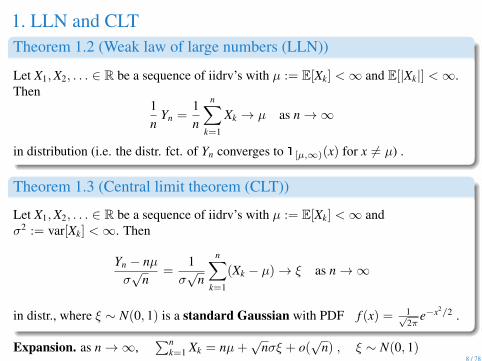
1. LLN and CLTTheorem 1.2 (Weak law of large numbers (LLN))
Let X1,X2, . . . ∈ R be a sequence of iidrv’s with µ := E[Xk] <∞ and E[|Xk|] <∞.Then
1n
Yn =1n
n∑k=1
Xk → µ as n→∞
in distribution (i.e. the distr. fct. of Yn converges to 1[µ,∞)(x) for x 6= µ) .
Theorem 1.3 (Central limit theorem (CLT))
Let X1,X2, . . . ∈ R be a sequence of iidrv’s with µ := E[Xk] <∞ andσ2 := var[Xk] <∞. Then
Yn − nµσ√
n=
1σ√
n
n∑k=1
(Xk − µ)→ ξ as n→∞
in distr., where ξ ∼ N(0, 1) is a standard Gaussian with PDF f (x) = 1√2π
e−x2/2 .
Expansion. as n→∞,∑n
k=1 Xk = nµ+√
nσξ + o(√
n) , ξ ∼ N(0, 1)8 / 78
1. Discrete-time Markov processesDefinition 1.4
A discrete-time stochastic process with state space S is a sequenceY0,Y1, . . . = (Yn : n ∈ N0) of random variables taking values in S.The process is called Markov, if for all A ⊆ S, n ∈ N0 and s0, . . . , sn ∈ S
A Markov process (MP) is called homogeneous if for all A ⊆ S, n ∈ N0 and s ∈ S
P(Yn+1 ∈ A|Yn = s) = P(Y1 ∈ A|Y0 = s) .
If S is discrete, the MP is called a Markov chain (MC).
The generic probability space Ω is the path space
Ω = D(N0, S) := SN0 = S× S× . . .
which is uncountable even when S is finite. For a given ω ∈ Ω the functionn 7→ Yn(ω) is called a sample path.Up to finite time N and with finite S, ΩN = SN+1 is finite.
9 / 78
1. Discrete-time Markov processes
Examples.For the simple random walk we have state space S = Z and Y0 = 0. Up to timeN, P is a distribution on the finite path space ΩN with
P(ω) =
p# of up-steps q# of down-steps , path ω possible
0 , path ω not possible
There are only 2N paths in ΩN with non-zero probability.For p = q = 1/2 they all have the same probability (1/2)N .
For the generalized random walk with Y0 = 0 and increments Yn+1 − Yn ∈ R, wehave S = R and ΩN = RN with an uncountable number of possible paths.
A sequence Y0,Y1, . . . ∈ S of iidrv’s is also a Markov process with state space S.
Let S = 1, . . . , 52 be a deck of cards, and Y1, . . . ,Y52 be the cards drawn atrandom without replacement. Is this a Markov process?
10 / 78
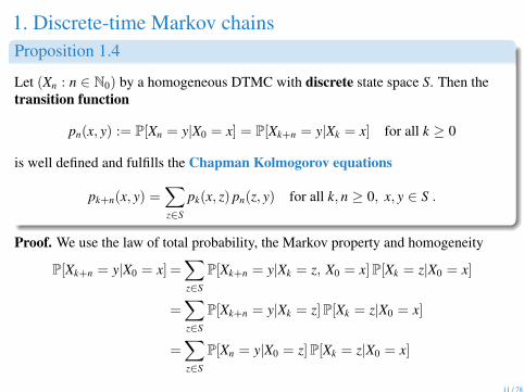
1. Discrete-time Markov chainsProposition 1.4
Let (Xn : n ∈ N0) by a homogeneous DTMC with discrete state space S. Then thetransition function
pn(x, y) := P[Xn = y|X0 = x] = P[Xk+n = y|Xk = x] for all k ≥ 0
is well defined and fulfills the Chapman Kolmogorov equations
pk+n(x, y) =∑z∈S
pk(x, z) pn(z, y) for all k, n ≥ 0, x, y ∈ S .
Proof. We use the law of total probability, the Markov property and homogeneity
P[Xk+n = y|X0 = x] =∑z∈S
P[Xk+n = y|Xk = z, X0 = x]P[Xk = z|X0 = x]
=∑z∈S
P[Xk+n = y|Xk = z]P[Xk = z|X0 = x]
=∑z∈S
P[Xn = y|X0 = z]P[Xk = z|X0 = x]
11 / 78
1. Markov chainsIn matrix form with Pn =
(pn(x, y) : x, y ∈ S
)the Chapman Kolmogorov
equations read
Pn+k = Pn Pk and in particular Pn+1 = Pn P1 .
With P0 = I, the obvious solution to this recursion is
Pn = Pn where we write P1 = P =(p(x, y) : x, y ∈ S
).
The transition matrix P and the initial condition X0 ∈ S completely determine ahomogeneous DTMC, since for all k ≥ 1 and all events A1, . . . ,Ak ⊆ S
P[X1 ∈ A1, . . . ,Xk ∈ Ak] =∑
s1∈A1
· · ·∑
sk∈Ak
p(X0, s1)p(s1, s2) · · · p(sk−1, sk) .
Fixed X0 can be replaced by an initial distribution π0(x) := P[X0 = x] .The distribution at time n is then
πn(x) =∑y∈S
∑s1∈S
· · ·∑
sn−1∈S
π0(y)p(y, s1) · · · p(sn−1, x) or 〈πn| = 〈π0|Pn .
12 / 78
1. Transition matricesThe transition matrix P is stochastic, i.e.
p(x, y) ∈ [0, 1] and∑
y
p(x, y) = 1 ,
or equivalently, the column vector |1〉 = (1, . . . , 1)T
is eigenvector with eigenvalue 1: P|1〉 = |1〉
Example 1 (Random walk with boundaries)Let (Xn : n ∈ N0) be a SRW on S = 1, . . . ,L with p(x, y) = pδy,x+1 + qδy,x−1.The boundary conditions are
periodic if p(L, 1) = p , p(1,L) = q ,absorbing if p(L,L) = 1 , p(1, 1) = 1 ,closed if p(1, 1) = q , p(L,L) = p ,reflecting if p(1, 2) = 1 , p(L,L− 1) = 1 .
13 / 78
1. Stationary distributions
Definition 1.5
Let (Xn : n ∈ N0) be a homogeneous DTMC with state space S. The distributionπ(x), x ∈ S is called stationary if for all y ∈ S∑
x∈S
π(x)p(x, y) = π(y) or 〈π|P = 〈π| .
π is called reversible if it fulfills the detailed balance conditions
π(x)p(x, y) = π(y)p(y, x) for all x, y ∈ S .
reversibility implies stationarity, since∑x∈S
π(x)p(x, y) =∑x∈S
π(y)p(y, x) = π(y) .
Stationary distributions as row vectors 〈π| = (π(x) : x ∈ S)
are left eigenvectors with eigenvalue 1: 〈π| = 〈π|P .
14 / 78
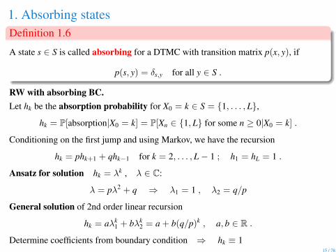
1. Absorbing statesDefinition 1.6
A state s ∈ S is called absorbing for a DTMC with transition matrix p(x, y), if
p(s, y) = δs,y for all y ∈ S .
RW with absorbing BC.Let hk be the absorption probability for X0 = k ∈ S = 1, . . . ,L,
hk = P[absorption|X0 = k] = P[Xn ∈ 1,L for some n ≥ 0|X0 = k] .
Conditioning on the first jump and using Markov, we have the recursion
hk = phk+1 + qhk−1 for k = 2, . . . ,L− 1 ; h1 = hL = 1 .
Ansatz for solution hk = λk , λ ∈ C:
λ = pλ2 + q ⇒ λ1 = 1 , λ2 = q/p
General solution of 2nd order linear recursion
hk = aλk1 + bλk
2 = a + b(q/p)k , a, b ∈ R .
Determine coefficients from boundary condition ⇒ hk ≡ 115 / 78
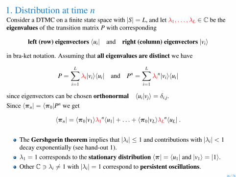
1. Distribution at time nConsider a DTMC on a finite state space with |S| = L, and let λ1, . . . , λL ∈ C be theeigenvalues of the transition matrix P with corresponding
left (row) eigenvectors 〈ui| and right (column) eigenvectors |vi〉
in bra-ket notation. Assuming that all eigenvalues are distinct we have
P =
L∑i=1
λi|vi〉〈ui| and Pn =
L∑i=1
λin|vi〉〈ui|
since eigenvectors can be chosen orthonormal 〈ui|vj〉 = δi,j.Since 〈πn| = 〈π0|Pn we get
〈πn| = 〈π0|v1〉λ1n〈u1|+ . . .+ 〈π0|vL〉λL
n〈uL| .
The Gershgorin theorem implies that |λi| ≤ 1 and contributions with |λi| < 1decay exponentially (see hand-out 1).λ1 = 1 corresponds to the stationary distribution 〈π| = 〈u1| and |v1〉 = |1〉.Other C 3 λi 6= 1 with |λi| = 1 correspond to persistent oscillations.
16 / 78
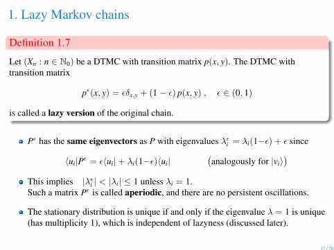
1. Lazy Markov chains
Definition 1.7
Let (Xn : n ∈ N0) be a DTMC with transition matrix p(x, y). The DTMC withtransition matrix
pε(x, y) = εδx,y + (1− ε) p(x, y) , ε ∈ (0, 1)
is called a lazy version of the original chain.
Pε has the same eigenvectors as P with eigenvalues λεi = λi(1−ε) + ε since
〈ui|Pε = ε〈ui|+ λi(1−ε)〈ui|(analogously for |vi〉
)This implies |λεi | < |λi| ≤ 1 unless λi = 1.Such a matrix Pε is called aperiodic, and there are no persistent oscillations.
The stationary distribution is unique if and only if the eigenvalue λ = 1 is unique(has multiplicity 1), which is independent of lazyness (discussed later).
17 / 78
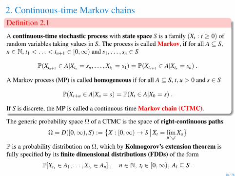
2. Continuous-time Markov chainsDefinition 2.1
A continuous-time stochastic process with state space S is a family (Xt : t ≥ 0) ofrandom variables taking values in S. The process is called Markov, if for all A ⊆ S,n ∈ N, t1 < . . . < tn+1 ∈ [0,∞) and s1, . . . , sn ∈ S
A Markov process (MP) is called homogeneous if for all A ⊆ S, t, u > 0 and s ∈ S
P(Xt+u ∈ A|Xu = s) = P(Xt ∈ A|X0 = s) .
If S is discrete, the MP is called a continuous-time Markov chain (CTMC).
The generic probability space Ω of a CTMC is the space of right-continuous paths
Ω = D([0,∞), S) :=
X : [0,∞)→ S∣∣Xt = lim
utXu
P is a probability distribution on Ω, which by Kolmogorov’s extension theorem isfully specified by its finite dimensional distributions (FDDs) of the form
P[Xt1 ∈ A1, . . . ,Xtn ∈ An] , n ∈ N, ti ∈ [0,∞), Ai ⊆ S .18 / 78
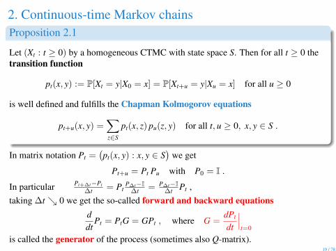
2. Continuous-time Markov chainsProposition 2.1
Let (Xt : t ≥ 0) by a homogeneous CTMC with state space S. Then for all t ≥ 0 thetransition function
pt(x, y) := P[Xt = y|X0 = x] = P[Xt+u = y|Xu = x] for all u ≥ 0
is well defined and fulfills the Chapman Kolmogorov equations
pt+u(x, y) =∑z∈S
pt(x, z) pu(z, y) for all t, u ≥ 0, x, y ∈ S .
In matrix notation Pt =(pt(x, y) : x, y ∈ S
)we get
Pt+u = Pt Pu with P0 = I .
In particular Pt+∆t−Pt∆t = Pt
P∆t−I∆t = P∆t−I
∆t Pt ,taking ∆t 0 we get the so-called forward and backward equations
ddt
Pt = PtG = GPt , where G =dPt
dt
∣∣∣t=0
is called the generator of the process (sometimes also Q-matrix).19 / 78
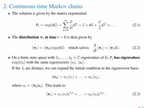
2. Continuous-time Markov chainsThe solution is given by the matrix exponential
Pt = exp(tG) =
∞∑k=0
tk
k!Gk = I + tG +
t2
2G2 + . . . (2.1)
The distribution πt at time t > 0 is then given by
〈πt| = 〈π0| exp(tG) which solvesddt〈πt| = 〈πt|G . (2.2)
On a finite state space with λ1, . . . , λL ∈ C eigenvalues of G, Pt has eigenvaluesexp(tλi) with the same eigenvectors 〈vi|, |ui〉.If the λi are distinct, we can expand the initial condition in the eigenvector basis
〈π0| = α1〈v1|+ . . .+ αL〈vL| ,
where αi = 〈π0|ui〉. This leads to
〈πt| = α1〈v1|eλ1t + . . .+ αL〈vL|eλLt . (2.3)
20 / 78
2. Continuous-time Markov chainsusing (2.1) we have for G =
(g(x, y) : x, y ∈ S
)p∆t(x, y) = g(x, y)∆t + o(∆t) for all x 6= y ∈ S .
So g(x, y) ≥ 0 can be interpreted as transition rates.
p∆t(x, x) = 1 + g(x, x)∆t + o(∆t) for all x ∈ S ,
and since∑
y p∆t(x, y) = 1 this implies that
g(x, x) = −∑y 6=x
g(x, y) ≤ 0 for all x ∈ S .
(2.2) can then be written intuitively as the Master equation
ddtπt(x) =
∑y 6=x
πt(y)g(y, x)
︸ ︷︷ ︸gain term
−∑y 6=x
πt(x)g(x, y)
︸ ︷︷ ︸loss term
for all x ∈ S .
The Gershgorin theorem now implies that either λi = 0 or Re(λi) < 0 for theeigenvalues of G, so there are no persistent oscillations for CTMCs.
21 / 78
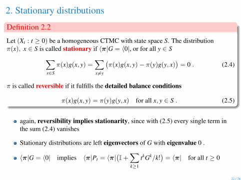
2. Stationary distributions
Definition 2.2
Let (Xt : t ≥ 0) be a homogeneous CTMC with state space S. The distributionπ(x), x ∈ S is called stationary if 〈π|G = 〈0|, or for all y ∈ S∑
x∈S
π(x)g(x, y) =∑x 6=y
(π(x)g(x, y)− π(y)g(y, x)
)= 0 . (2.4)
π is called reversible if it fulfills the detailed balance conditions
π(x)g(x, y) = π(y)g(y, x) for all x, y ∈ S . (2.5)
again, reversibility implies stationarity, since with (2.5) every single term inthe sum (2.4) vanishes
Stationary distributions are left eigenvectors of G with eigenvalue 0 .
〈π|G = 〈0| implies 〈π|Pt = 〈π|(I +
∑k≥1
tkGk/k!)
= 〈π| for all t ≥ 0
22 / 78
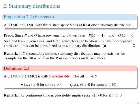
2. Stationary distributions
Proposition 2.2 (Existence)
A DTMC or CTMC with finite state space S has at least one stationary distribution.
Proof. Since P and G have row sum 1 and 0 we have P|1〉 = |1〉 and G|1〉 = |0〉So 1 and 0 are eigenvalues, and left eigenvectors can be shown to have non-negativeentries and thus can be normalized to be stationary distributions 〈π|. 2
Remark. If S is countably infinite, stationary distributions may not exist, as forexample for the SRW on Z or the Poisson process on N (see later).
Definition 2.3
A CTMC (or DTMC) is called irreducible, if for all x, y ∈ S
pt(x, y) > 0 for some t > 0 (pn(x, y) > 0 for some n ∈ N) .
Remark. For continuous time irreducibility implies pt(x, y) > 0 for all t > 0.
23 / 78
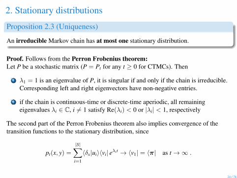
2. Stationary distributions
Proposition 2.3 (Uniqueness)
An irreducible Markov chain has at most one stationary distribution.
Proof. Follows from the Perron Frobenius theorem:Let P be a stochastic matrix (P = Pt for any t ≥ 0 for CTMCs). Then
1 λ1 = 1 is an eigenvalue of P, it is singular if and only if the chain is irreducible.Corresponding left and right eigenvectors have non-negative entries.
2 if the chain is continuous-time or discrete-time aperiodic, all remainingeigenvalues λi ∈ C, i 6= 1 satisfy Re(λi) < 0 or |λi| < 1, respectively
The second part of the Perron Frobenius theorem also implies convergence of thetransition functions to the stationary distribution, since
pt(x, y) =
|S|∑i=1
〈δx|ui〉〈vi| eλit → 〈v1| = 〈π| as t→∞ .
24 / 78
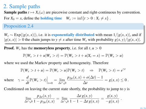
2. Sample pathsSample paths t 7→ Xt(ω) are piecewise constant and right-continuous by convention.For X0 = x, define the holding time Wx := inft > 0 : Xt 6= x .
Proposition 2.4
Wx ∼ Exp(|g(x, x)|), i.e. it is exponentially distributed with mean 1/|g(x, x)|, and if|g(x, x)| > 0 the chain jumps to y 6= x after time Wx with probability g(x, y)/|g(x, x)|.
Proof. Wx has the memoryless property, i.e. for all t, u > 0
P(Wx > t + u|Wx > t) = P(Wx > t + u|Xt = x) = P(Wx > u)
where we used the Markov property and homogeneity. Therefore
Conditioned on leaving the current state shortly, the probability to jump to y is
lim∆t0
p∆t(x, y)
1− p∆t(x, x)= lim
∆t0
∆t g(x, y)
1− 1−∆t g(x, x)=
g(x, y)
−g(x, x).
25 / 78
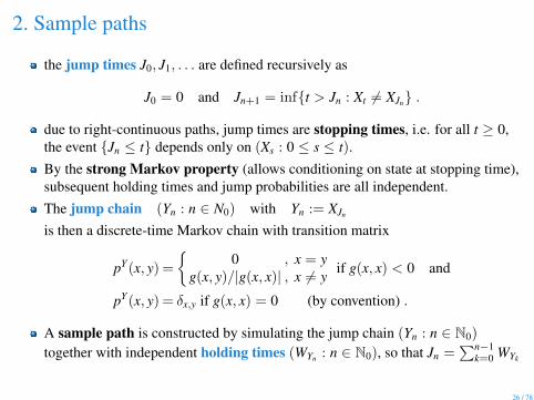
2. Sample paths
the jump times J0, J1, . . . are defined recursively as
J0 = 0 and Jn+1 = inft > Jn : Xt 6= XJn .
due to right-continuous paths, jump times are stopping times, i.e. for all t ≥ 0,the event Jn ≤ t depends only on (Xs : 0 ≤ s ≤ t).By the strong Markov property (allows conditioning on state at stopping time),subsequent holding times and jump probabilities are all independent.The jump chain (Yn : n ∈ N0) with Yn := XJn
is then a discrete-time Markov chain with transition matrix
pY(x, y) =
0 , x = y
g(x, y)/|g(x, x)| , x 6= y if g(x, x) < 0 and
pY(x, y) = δx,y if g(x, x) = 0 (by convention) .
A sample path is constructed by simulating the jump chain (Yn : n ∈ N0)
together with independent holding times (WYn : n ∈ N0), so that Jn =∑n−1
k=0 WYk
26 / 78
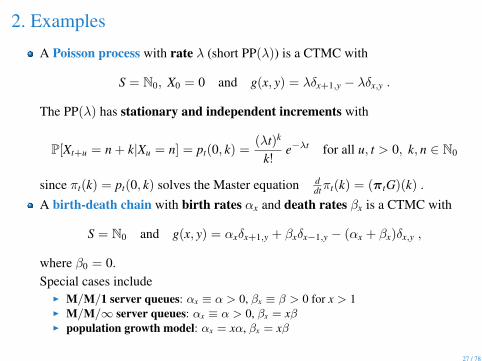
2. Examples
A Poisson process with rate λ (short PP(λ)) is a CTMC with
S = N0, X0 = 0 and g(x, y) = λδx+1,y − λδx,y .
The PP(λ) has stationary and independent increments with
P[Xt+u = n + k|Xu = n] = pt(0, k) =(λt)k
k!e−λt for all u, t > 0, k, n ∈ N0
since πt(k) = pt(0, k) solves the Master equation ddtπt(k) = (πtG)(k) .
A birth-death chain with birth rates αx and death rates βx is a CTMC with
S = N0 and g(x, y) = αxδx+1,y + βxδx−1,y − (αx + βx)δx,y ,
where β0 = 0.Special cases include
I M/M/1 server queues: αx ≡ α > 0, βx ≡ β > 0 for x > 1I M/M/∞ server queues: αx ≡ α > 0, βx = xβI population growth model: αx = xα, βx = xβ
27 / 78
2. ErgodicityDefinition 2.4
A Markov process is called ergodic if it has a unique stationary distribution π and
pt(x, y) = P[Xt = y|X0 = x]→ π(y) as t→∞ , for all x, y ∈ S .
Theorem 2.5
An irreducible (aperiodic) MC with finite state space is ergodic.
Theorem 2.6 (Ergodic Theorem)
Consider an ergodic Markov chain with unique stationary distribution π. Then forevery bounded function f : S→ R we have with probability 1
1T
∫ T
0f (Xt) dt or
1N
N∑n=1
f (Xn) → Eπ[f ] as T,N →∞ .
for a proof see e.g. [GS], chapter 9.5in practice, use relaxation/burn-in time before computing time averages
28 / 78
2. Markov Chain Monte Carlo (MCMC)Typical problems related to sampling from π on a very large state space S
Compute expectations Eπ[f ] =∑
x∈S f (x)π(x)
for Gibbs measures π(x) = 1Z(β) e−βH(x) (stach. mech. problems),
compute partition function Z(β) =∑
x∈S e−βH(x)
Use the ergodic theorem to estimate expectations by time averagesassume π(x) > 0 for all x ∈ S (otherwise restrict S)invent CTMC/DTMC such that π is stationary, e.g. via detailed balance
for Gibbs measures e−βH(x)g(x, y) = e−βH(y)g(y, x)
Typically g(x, y) = q(x, y) a(x, y) , i.e. propose move from x to y with rateq(x, y) = q(y, x) (irreducible on S but ’local’), accept with probability a(x, y)
Heat bath algorithm: a(x, y) =e−βH(y)
e−βH(x) + e−βH(y)
Metropolis-Hastings: a(x, y) =
1 , if H(y) ≤ H(x)
eβ(H(x)−H(y)) , if H(y) > H(x)
29 / 78
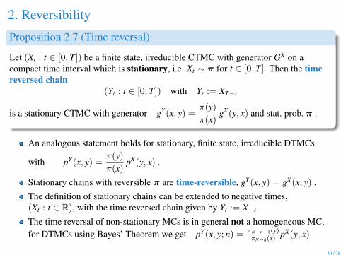
2. Reversibility
Proposition 2.7 (Time reversal)
Let (Xt : t ∈ [0,T]) be a finite state, irreducible CTMC with generator GX on acompact time interval which is stationary, i.e. Xt ∼ π for t ∈ [0,T]. Then the timereversed chain
(Yt : t ∈ [0,T]) with Yt := XT−t
is a stationary CTMC with generator gY(x, y) =π(y)
π(x)gX(y, x) and stat. prob. π .
An analogous statement holds for stationary, finite state, irreducible DTMCs
with pY(x, y) =π(y)
π(x)pX(y, x) .
Stationary chains with reversible π are time-reversible, gY(x, y) = gX(x, y) .The definition of stationary chains can be extended to negative times,(Xt : t ∈ R), with the time reversed chain given by Yt := X−t.The time reversal of non-stationary MCs is in general not a homogeneous MC,for DTMCs using Bayes’ Theorem we get pY(x, y; n) = πN−n−1(y)
πN−n(x) pX(y, x)
30 / 78
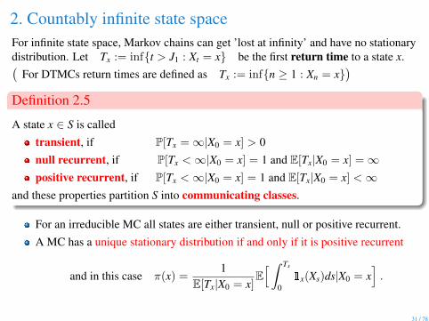
2. Countably infinite state spaceFor infinite state space, Markov chains can get ’lost at infinity’ and have no stationarydistribution. Let Tx := inft > J1 : Xt = x be the first return time to a state x.(
For DTMCs return times are defined as Tx := infn ≥ 1 : Xn = x)
Definition 2.5
A state x ∈ S is calledtransient, if P[Tx =∞|X0 = x] > 0null recurrent, if P[Tx <∞|X0 = x] = 1 and E[Tx|X0 = x] =∞positive recurrent, if P[Tx <∞|X0 = x] = 1 and E[Tx|X0 = x] <∞
and these properties partition S into communicating classes.
For an irreducible MC all states are either transient, null or positive recurrent.A MC has a unique stationary distribution if and only if it is positive recurrent
and in this case π(x) =1
E[Tx|X0 = x]E[ ∫ Tx
01x(Xs)ds|X0 = x
].
31 / 78
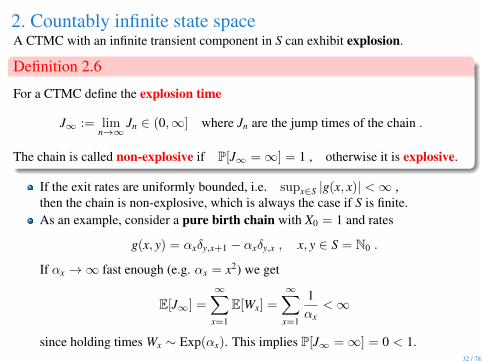
2. Countably infinite state spaceA CTMC with an infinite transient component in S can exhibit explosion.
Definition 2.6
For a CTMC define the explosion time
J∞ := limn→∞
Jn ∈ (0,∞] where Jn are the jump times of the chain .
The chain is called non-explosive if P[J∞ =∞] = 1 , otherwise it is explosive.
If the exit rates are uniformly bounded, i.e. supx∈S |g(x, x)| <∞ ,then the chain is non-explosive, which is always the case if S is finite.As an example, consider a pure birth chain with X0 = 1 and rates
g(x, y) = αxδy,x+1 − αxδy,x , x, y ∈ S = N0 .
If αx →∞ fast enough (e.g. αx = x2) we get
E[J∞] =
∞∑x=1
E[Wx] =
∞∑x=1
1αx
<∞
since holding times Wx ∼ Exp(αx). This implies P[J∞ =∞] = 0 < 1.32 / 78
3. Markov processes with S = RProposition 3.1
Let (Xt : t ≥ 0) by a homogeneous MP as in Definition 18 with state space S = R.Then for all t ≥ 0 and (measurable) A ⊆ R the transition kernel for all x ∈ R
Pt(x,A) := P[Xt ∈ A|X0 = x] = P[Xt+u ∈ A|Xu = x] for all u ≥ 0
is well defined. If it is absolutely continuous the transition density pt with
Pt(x,A) =
∫A
pt(x, y) dy
exists and fulfills the Chapman Kolmogorov equations
pt+u(x, y) =
∫R
pt(x, z) pu(z, y) dz for all t, u ≥ 0, x, y ∈ R .
As for CTMCs, the transition densities and the initial distribution p0(x) describe allfinite dimensional distributions (fdds)
P[Xt1 ≤ x1, . . . ,Xtn ≤ xn] =
∫R
dz0p0(z0)
∫ x1
−∞dz1pt1(z0, z1) · · ·
∫ xn
−∞dznptn−tn−1(zn−1, zn)
for all n ∈ N, 0 < t1 < . . . < tn and x1, . . . xn ∈ R.33 / 78
3. Jump processes(Xt : t ≥ 0) is a jump process with state space S = R characterized by ajump rate density r(x, y) ≥ 0 with a uniformly boundedtotal exit rate R(x) =
∫R r(x, y) dy < R <∞ for all x ∈ R .
Ansatz for transition function as ∆t→ 0:
p∆t(z, y) = r(z, y)∆t +(1− R(z)∆t
)δ(y− z)
Then use the Chapman Kolmogorov equations
pt+∆t(x, y)− pt(x, y) =
∫R
pt(x, z) p∆t(z, y) dz− pt(x, y) =
=
∫R
pt(x, z)r(z, y)∆t dz +
∫R
(1− R(z)∆t − 1
)pt(x, z)δ(y− z)dz
to get the Kolmogorov-Feller equation (x is a fixed initial condition)
∂
∂tpt(x, y) =
∫R
(pt(x, z)r(z, y)− pt(x, y)r(y, z)
)dz .
As for CTMC sample paths t 7→ Xt(ω) are piecewise constant and right-continuous.34 / 78
3. Gaussian processesX = (X1, . . . ,Xn) ∼ N (µ,Σ) is a multivariate Gaussian in Rn if it has PDF
f (x) =1√
(2π)n det Σexp
(− 1
2〈x− µ|Σ−1 |x− µ〉
),
with mean µ = (µ1, . . . , µn) ∈ Rn and covariance matrix
A stochastic process (Xt : t ≥ 0) with state space S = R is a Gaussian process if forall n ∈ N, 0 ≤ t1 < . . . < tn the vector (Xt1 , . . . ,Xtn) is a multivariate Gaussian.
Proposition 3.2
All fdds of a Gaussian process (Xt : t ≥ 0) are fully characterized by the mean andthe covariance function
m(t) := E[Xt] and σ(s, t) := Cov[Xs,Xt] .
35 / 78
3. Stationary independent increments
Definition 3.2
A stochastic process (Xt : t ≥ 0) has stationary increments if
Xt − Xs ∼ Xt−s − X0 for all 0 ≤ s ≤ t .
It has independent increments if for all n ≥ 1 and 0 ≤ t1 < · · · < tnXtk+1 − Xtk : 1 ≤ k < n
are independent .
Example. The Poisson process (Nt : t ≥ 0) ∼ PP(λ) has stationary independentincrements with Nt − Ns ∼ Poi
(λ(t − s)
).
Proposition 3.3
The following two statements are equivalent for a stochastic process (Xt : t ≥ 0):Xt has stationary independent increments and Xt ∼ N (0, t) for all t ≥ 0.Xt is a Gaussian process with m(t) = 0 and σ(s, t) = mins, t.
Stationary independent incr. have stable distributions such as Gaussian or Poisson.36 / 78
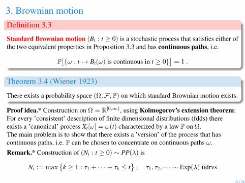
3. Brownian motionDefinition 3.3
Standard Brownian motion (Bt : t ≥ 0) is a stochastic process that satisfies either ofthe two equivalent properties in Proposition 3.3 and has continuous paths, i.e.
P[ω : t 7→ Bt(ω) is continuous in t ≥ 0
]= 1 .
Theorem 3.4 (Wiener 1923)
There exists a probability space (Ω,F ,P) on which standard Brownian motion exists.
Proof idea.* Construction on Ω = R[0,∞), using Kolmogorov’s extension theorem:For every ’consistent’ description of finite dimensional distributions (fdds) thereexists a ’canonical’ process Xt[ω] = ω(t) characterized by a law P on Ω.The main problem is to show that there exists a ’version’ of the process that hascontinuous paths, i.e. P can be chosen to concentrate on continuous paths ω.Remark.* Construction of (Nt : t ≥ 0) ∼ PP(λ) is
3. Properties of Brownian motionSBM is a time-homogeneous MP with B0 = 0.σBt + x with σ > 0 is a (general) BM with Bt ∼ N (x, σ2t).The transition density is given by a Gaussion PDF
pt(x, y) =1√
2πσ2texp
(− (y− x)2
2σ2t
)This is also called the heat kernel, since it solves the heat/diffusion equation
∂
∂tpt(x, y) =
σ2
2∂2
∂y2 pt(x, y) with p0(x, y) = δ(y− x) .
SBM is self-similar with Hurst exponent H = 1/2, i.e.
(Bλt : t ≥ 0) ∼ λH(Bt : t ≥ 0) for all λ > 0 .
t 7→ Bt is P− a.s. not differentiable at t for all t ≥ 0.For fixed h > 0 define ξh
t := (Bt+h − Bt)/h ∼ N (0, 1/h), which is a mean-0
Gaussian process with covariance σ(s, t) =
0 , |t − s| > h
(h− |t − s|)/h2 , |t − s| < h .
The (non-existent) derivative ξt := limh→0
ξht is called white noise and is formally a
mean-0 Gaussian process with covariance σ(s, t) = δ(t − s).38 / 78
3. Generators as operatorsFor a CTMC (Xt : t ≥ 0) with discrete state space S we have for f : S→ R
E[f (Xt)
]=∑x∈S
πt(x)f (x) = 〈πt|f 〉 andddt〈πt| = 〈πt|G︸ ︷︷ ︸
master equation
ThereforeddtE[f (Xt)
]=
ddt〈πt|f 〉 = 〈πt|G|f 〉 = E
[(Gf )(Xt)
].
The generator G can be defined as an operator G acting on functions f : S→ R
G|f 〉(x) = (G f )(x) =∑y6=x
g(x, y)[f (y)− f (x)
].
For Brownian motion use the heat eq. and integration by parts for f ∈ C2(R)
ddtEx[f (Xt)
]=
∫R∂tpt(x, y)f (y)dy =
σ2
2
∫R∂2
y pt(x, y)f (y)dy = Ex[(Lf )(Xt)
]where the generator of BM is (Lf )(x) =
σ2
2∆f (x)
(orσ2
2f ′′(x)
).
For jump processes with S = R and rate density r(x, y) the generator is
(Lf )(x) =
∫R
r(x, y)[f (y)− f (x)
]dy .
39 / 78
3. Brownian motion as scaling limit
Proposition 3.5
Let (Xt : t ≥ 0) be a jump process on R with translation invariant ratesr(x, y) = q(y− x) which have
mean zero∫R
q(z) z dz = 0 and
finite second moment σ2 :=
∫R
q(z) z2 dz <∞ .
Then for all T > 0 the rescaled process(εXt/ε2 : t ∈ [0,T]
)⇒
(Bt : t ∈ [0,T]
)as ε→ 0
converges in distribution to a BM with generator L = 12σ
2∆ for all T > 0.
Proof. Taylor expansion of the generator for test functions f ∈ C3(R), and tightnessargument for continuity of paths (requires fixed interval [0,T]).
40 / 78
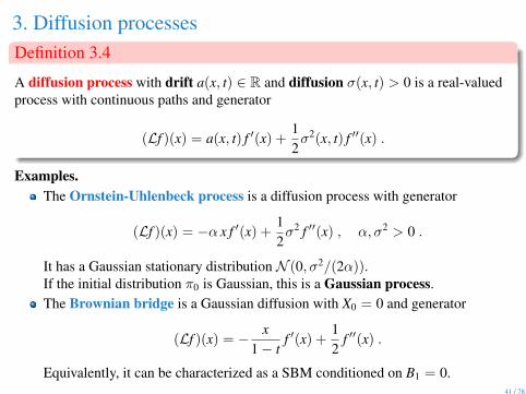
3. Diffusion processesDefinition 3.4
A diffusion process with drift a(x, t) ∈ R and diffusion σ(x, t) > 0 is a real-valuedprocess with continuous paths and generator
(Lf )(x) = a(x, t) f ′(x) +12σ2(x, t) f ′′(x) .
Examples.The Ornstein-Uhlenbeck process is a diffusion process with generator
(Lf )(x) = −α x f ′(x) +12σ2 f ′′(x) , α, σ2 > 0 .
It has a Gaussian stationary distribution N (0, σ2/(2α)).If the initial distribution π0 is Gaussian, this is a Gaussian process.The Brownian bridge is a Gaussian diffusion with X0 = 0 and generator
(Lf )(x) = − x1− t
f ′(x) +12
f ′′(x) .
Equivalently, it can be characterized as a SBM conditioned on B1 = 0.41 / 78
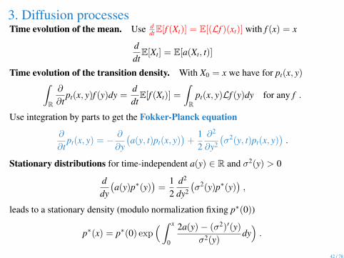
3. Diffusion processesTime evolution of the mean. Use d
dtE[f (Xt)] = E[(Lf )(xt)] with f (x) = x
ddtE[Xt] = E[a(Xt, t)]
Time evolution of the transition density. With X0 = x we have for pt(x, y)∫R
∂
∂tpt(x, y)f (y)dy =
ddtE[f (Xt)] =
∫R
pt(x, y)Lf (y)dy for any f .
Use integration by parts to get the Fokker-Planck equation
∂
∂tpt(x, y) = − ∂
∂y
(a(y, t)pt(x, y)
)+
12∂2
∂y2
(σ2(y, t)pt(x, y)
).
Stationary distributions for time-independent a(y) ∈ R and σ2(y) > 0
ddy
(a(y)p∗(y)
)=
12
d2
dy2
(σ2(y)p∗(y)
),
leads to a stationary density (modulo normalization fixing p∗(0))
p∗(x) = p∗(0) exp(∫ x
0
2a(y)− (σ2)′(y)
σ2(y)dy).
42 / 78
3. Beyond diffusionDefinition 3.5
A Levy process (Xt : t ≥ 0) is a real-valued process with right-continuous paths andstationary, independent increments.
The generator has a part with constant drift a ∈ R and diffusion σ2 ≥ 0
Lf (x) = af ′(x) +σ2
2f ′′(x) +
∫R
(f (x + z)− f (x)− zf ′(x)1(0,1)(|z|)
)q(z)dz ,
and a translation invariant jump part with density q(z) (or measure ν(dz))
and fulfills∫|z|>1
q(z)dz <∞ and∫
0<|z|<1z2q(z)dz <∞ .
Diffusion processes, in particular BM with a = 0, σ2 > 0 and q(z) ≡ 0, or jumpprocesses, in particular Poisson with a = σ = 0 and q(z) = λδ(z− 1).For a = σ = 0 and heavy-tailed jump distribution
q(z) = C|z|1+α with C > 0 and α ∈ (0, 2]
the process is called α-stable symmetric Levy process or Levy flight.self-similar (Xλt : t ≥ 0) ∼ λH(Xt : t ≥ 0) , λ > 0 with H = 1/α⇒ super-diffusive behaviour with E[X2
t ] ∝ t2/α
43 / 78
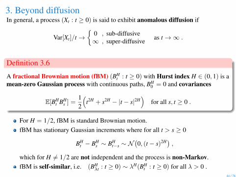
3. Beyond diffusionIn general, a process (Xt : t ≥ 0) is said to exhibit anomalous diffusion if
Var[Xt]/t→
0 , sub-diffusive∞ , super-diffusive as t→∞ .
Definition 3.6
A fractional Brownian motion (fBM) (BHt : t ≥ 0) with Hurst index H ∈ (0, 1) is a
mean-zero Gaussian process with continuous paths, BH0 = 0 and covariances
E[BHt BH
s ] =12
(t2H + s2H − |t − s|2H
)for all s, t ≥ 0 .
For H = 1/2, fBM is standard Brownian motion.fBM has stationary Gaussian increments where for all t > s ≥ 0
BHt − BH
s ∼ BHt−s ∼ N
(0, (t − s)2H) ,
which for H 6= 1/2 are not independent and the process is non-Markov.fBM is self-similar, i.e. (BH
λt : t ≥ 0) ∼ λH(BHt : t ≥ 0) for all λ > 0 .
44 / 78
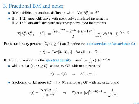
3. Fractional BM and noisefBM exhibits anomalous diffusion with Var[BH
t ] = t2H
H > 1/2: super-diffusive with positively correlated incrementsH < 1/2: sub-diffusive with negatively correlated increments
E[BH
1 (BHt+1 − BH
t )]
=(t+1)2H − 2t2H + (t−1)2H
2'
t→∞H(2H−1)t2(H−1)
For a stationary process(Xt : t ≥ 0
)on R define the autocorrelation/covariance fct
c(t) := Cov[Xs,Xs+t] for all s, t ∈ R .
Its Fourier transform is the spectral density S(ω) :=∫R c(t)e−iωtdt
white noise (ξt : t ≥ 0), stationary GP with mean zero and
c(t) = δ(t) ⇒ S(ω) ≡ 1 .
fractional or 1/f noise (ξHt : t ≥ 0), stationary GP with mean zero and
c(t) =2H(2H−1)
|t|2(1−H)⇒ S(ω) ∝ |ω|2(1−H)−1 =
1ω2H−1
45 / 78
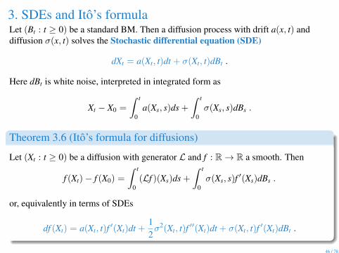
3. SDEs and Ito’s formulaLet (Bt : t ≥ 0) be a standard BM. Then a diffusion process with drift a(x, t) anddiffusion σ(x, t) solves the Stochastic differential equation (SDE)
dXt = a(Xt, t)dt + σ(Xt, t)dBt .
Here dBt is white noise, interpreted in integrated form as
Xt − X0 =
∫ t
0a(Xs, s)ds +
∫ t
0σ(Xs, s)dBs .
Theorem 3.6 (Ito’s formula for diffusions)
Let (Xt : t ≥ 0) be a diffusion with generator L and f : R→ R a smooth. Then
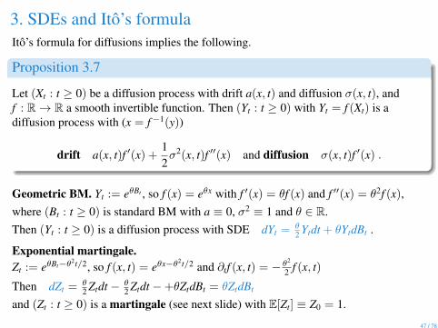
3. SDEs and Ito’s formulaIto’s formula for diffusions implies the following.
Proposition 3.7
Let (Xt : t ≥ 0) be a diffusion process with drift a(x, t) and diffusion σ(x, t), andf : R→ R a smooth invertible function. Then (Yt : t ≥ 0) with Yt = f (Xt) is adiffusion process with (x = f−1(y))
Geometric BM. Yt := eθBt , so f (x) = eθx with f ′(x) = θf (x) and f ′′(x) = θ2f (x),where (Bt : t ≥ 0) is standard BM with a ≡ 0, σ2 ≡ 1 and θ ∈ R.Then (Yt : t ≥ 0) is a diffusion process with SDE dYt = θ
2 Ytdt + θYtdBt .
Exponential martingale.Zt := eθBt−θ2t/2, so f (x, t) = eθx−θ2t/2 and ∂tf (x, t) = − θ
2
2 f (x, t)
Then dZt = θ2 Ztdt − θ
2 Ztdt −+θZtdBt = θZtdBt
and (Zt : t ≥ 0) is a martingale (see next slide) with E[Zt] ≡ Z0 = 1.
47 / 78
3. Fluctuations and martingalesDefinition 3.7
A real-valued stochastic process (Mt : t ≥ 0) is a martingale w.r.t. the process(Xt : t ≥ 0) if for all t ≥ 0 we have E[|Mt|] <∞ and
E[Mt∣∣Xu : 0 ≤ u ≤ s
]= Ms a.s. for all s ≤ t .
If in addition E[M2t ] <∞, there exists a unique increasing process ([M]t : t ≥ 0)
called the quadratic variation, with [M]0 = 0 and such that M2t − [M]t is martingale.
Theorem 3.8 (Ito’s formula)
Let (Xt : t ≥ 0) be a Markov process on state space S with generator L. Then for anysmooth enough f : S× [0,∞)→ R
f (Xt, t)− f (X0, 0) =
∫ t
0(Lf )(Xs, s)ds +
∫ t
0∂sf (Xs, s)ds + Mf
t ,
where (Mft : t ≥ 0) is a martingale w.r.t. (Xt : t ≥ 0) with Mf
0 = 0 and
quadratic variation [Mf ]t =
∫ t
0
((Lf 2)(Xs, s)− 2(fLf )(Xs, s)
)ds .
48 / 78
3. Fluctuations and martingalesFor a Poisson process (Nt : t ≥ 0) with rate λ > 0 Ito’s formula implies that
Mt := Nt − λt is a martingale with quadr. variation [M]t = λt .
Watanabe’s characterication of PP: Let (Nt : t ≥ 0) be a counting process,i.e. a jump process on S = N with jump size +1 only. If Mt = Nt − λt is amartingale, then (Nt : t ≥ 0) ∼ PP(λ).For a diffusion process, choosing f (Xt, t) = Xt in Ito’s formula leads to
Xt − X0 =
∫ t
0a(Xs, s)ds + Mt with [M]t =
∫ t
0σ2(Xs, s)ds .
In particular for BM with a(x, t) ≡ 0 and σ2(x, t) ≡ σ2 we have
(Bt : t ≥ 0) is a martingale with quadratic variation [B]t = t .
Levy’s characterication of BM: Any continuous martingale (Mt : t ≥ 0) on Rwith M0 = 0 and quadratic variation [M]t = t is standard Brownian motion.
Furthermore, any continuous martingale (Mt : t ≥ 0) on R with M0 = 0 is acontinuous (random) time-change of a standard BM, i.e.
(Mt : t ≥ 0) ∼(B[M]t : t ≥ 0
)for SBM (Bt : t ≥ 0) .
49 / 78
3. Fluctuations and martingalesFor a diffusion process (Xt : t ≥ 0) we have
Xt − X0 =
∫ t
0a(Xs, s)ds + Mt with [M]t =
∫ t
0σ2(Xs, s)ds .
with Mt a continuous martingale ⇒ (Mt : t ≥ 0) ∼ (B[M]t : t ≥ 0)
Related time-changed BMs can be written as stochastic Ito integrals
Mt =
∫ t
0σ(Xs, s)dBs := B[M]t .
Therefore σ ≡ 0 implies deterministic dynamics with Mt ≡ 0,(also because Lf 2 = 2f f ′a = 2fLf for all f , so [Mf ]t ≡ 0 in Ito’s formula)and the corresponding SDE is an ODE dXt/dt = a(Xt, t) .
Vanishing drift a ≡ 0 implies Xt − X0 = Mt or dXt = σ(Xt, t)dBt
and the process (Xt : t ≥ 0) is a martingale.
Recall the exponential martingale eθBt−θ2t/2 as a non-trivial example.
50 / 78
3. Martingales and conservation lawsConsider a CTMP (Xt : t ≥ 0) on state space S with generator L, and an observablef : S→ R such that Lf : S→ R is well defined (e.g. f ∈ C2(S,R) for diffusions).
Proposition 3.9
If Lf (x) = 0 for all x ∈ S, then f (Xt) is a martingale, and is conserved inexpectation, i.e. (for any initial condition X0)
E[f (Xt)
]= E
[f (X0)
]for all t ≥ 0 .
If in addition Lf 2(x) = 0 for all x ∈ S, then f (Xt) is conserved (or a conservedquantity), i.e. (for any initial condition X0)
f (Xt) = f (X0) almost surely for all t ≥ 0 .
Proof. The first claim follows directly from Ito’s formula (Theorem 3.8).For the second claim, we have f (Xt) = f (X0) + Mf
t and Mft has quadratic variation
[Mf ]t =
∫ t
0
((Lf 2)(Xs, s)− 2(fLf )(Xs, s)
)ds = 0 ,
for all t ≥ 0, which implies Mft ≡ 0 almost surely. 2
51 / 78
4. Stochastic particle systemslattice/population: Λ = 1, . . . ,L , finite set of pointsstate space S is given by the set of all configurations
η =(η(i) : i ∈ Λ
)∈ S = 0, 1L (often also written 0, 1Λ) .
η(i) ∈ 0, 1 signifies the presence of a particle/infection at site/individual i.Only local transitions are allowed with rates
η → ηi with rate c(η, ηi) (reaction)η → ηij with rate c(η, ηij) (transport)
where ηi(k) =
η(k) , k 6= i
1− η(k) , k = i and ηij(k) =
η(k) , k 6= i, jη(j) , k = iη(i) , k = j
Definition 4.1
A stochastic particle system is a CTMC with state space S = 0, 1Λ and generator
Lf (η) =∑i∈Λ
c(η, ηi)[f (ηi)− f (η)
]or Lf (η) =
∑i,j∈Λ
c(η, ηij)[f (ηij)− f (η)
].
52 / 78
4. Contact processThe contact process is a simple stochastic model for the SI epidemic with infectionrates q(i, j) ≥ 0 and uniform recovery rate 1.
Definition 4.2
The contact process (CP) (ηt : t ≥ 0) is an IPS with rates
c(η, ηi) = 1 · δη(i),1︸ ︷︷ ︸recovery
+ δη(i),0
∑j6=i
q(j, i)δη(j),1︸ ︷︷ ︸infection
for all i ∈ Λ .
Usually, q(i, j) = q(j, i) ∈ 0, λ, i.e. connected individuals infect each other withfixed rate λ > 0.
The CP has one absorbing state η(i) = 0 for all i ∈ Λ, which can be reachedfrom every initial configuration. Therefore the process is ergodic and theinfection eventually gets extinct with probability 1.Let T := inft > 0 : ηt ≡ 0 be the extinction time. Then there exists a criticalvalue (epidemic threshold) λc > 0 such that (for irreducible q(i, j))
E[T|η0 ≡ 1] ∝ log L for λ < λc and E[T|η0 ≡ 1] ∝ eC L for λ > λc .
53 / 78
4. Voter modelThe voter model describes opinion dynamics with influence rates q(i, j) ≥ 0 at whichindividual i persuades j to switch to her/his opinion.
Definition 4.3
The linear voter model (VM) (ηt : t ≥ 0) is an IPS with rates
c(η, ηi) =∑j 6=i
q(j, i)(δη(i),1δη(j),0 + δη(i),0δη(j),1
)︸ ︷︷ ︸j influences i if opinions differ
for all i ∈ Λ .
In non-linear versions the rates can be replaced by general (symmetric) functions.
The VM is symmetric under relabelling opinions 0↔ 1.If q(i, j) is irreducible there are two absorbing states, η ≡ 0, 1, both of which canbe reached from every initial condition. Therefore the VM is not ergodic, andstationary measures are
αδ0 + (1− α)δ1 with α ∈ [0, 1] depending on the initial condition .
Coexistence of both opinions can occur on infinite lattices (e.g. Zd for d ≥ 3).54 / 78
4. Exclusion processThe exclusion process describes transport of a conserved quantity (e.g. mass orenergy) with transport rates q(i, j) ≥ 0 site i to j.
Definition 4.4
The exclusion process (EP) (ηt : t ≥ 0) is an IPS with rates
c(η, ηij) = q(i, j)δη(i),1δη(j),0 for all i, j ∈ Λ .
The EP is called simple (SEP) if jumps occur only between nearest neighbours on Λ.The SEP is symmetric (SSEP) if q(i, j) = q(j, i), otherwise asymmetric (ASEP).
The SEP is mostly studied in a 1D geometry with periodic or open boundaries.For periodic boundary conditions the total number of particles N =
∑i η(i) is
conserved. The process is ergodic on the sub-state space
SN =η ∈ 0, 1L :
∑i
η(i) = N
for each value N = 0, . . .L, and has a unique stationary distribution.For open boundaries particles can be created and destroyed at the boundary, thesystem is ergodic on S and has a unique stationary distribution.
55 / 78
4. Mean-field scaling limitsConsider the contact process (ηt : t ≥ 0) on a complete graph, using η(i) ∈ 0, 1we can write the generator as
Lf (η) =∑i∈Λ
(η(i) + λ
(1− η(i)
)∑j∈Λ
η(j))[
f (ηi)− f (η)].
For mean-field observables such as N(η) :=∑
i∈Λ η(i) one can compute forf : N0 → R (see problem sheet 3)
L(f N)(η) = λ(L− N
)N[f (N + 1)− f (N)
]+ N
[f (N − 1)− f (N)
],
which shows that t 7→ Nt := N(ηt) is a Markov process with above generator for all L.
Mean-field scaling limit. L→∞ with λL→ λ
then Nt/L→ Xt, which is a diffusion process on [0, 1] with generator
Lf (x) =(λx(1− x)− x
)f ′(x) +
12L
(λx(1− x) + x
)f ′′(x)
In the limit the diffusion coefficient vanishes and the process is deterministic (blue)with leading order diffusive correction (red) and corresponding SDE
dXt =(λXt(1− Xt)− Xt
)dt +
√1L
(λXt(1− Xt) + Xt
)dBt
56 / 78
5. Graphs - definition
Definition 5.1
A graph (or network) G = (V,E) consists of a finite set V = 1, . . . ,N of vertices(or nodes, points), and a set E ⊆ V × V of edges (or links, lines).The graph is called undirected if (i, j) ∈ E implies (j, i) ∈ E, otherwise directed.The structure of the graph is encoded in the adjacency (or connectivity) matrix
A = (aij : i, j ∈ V) where aij =
1 , (i, j) ∈ E0 , (i, j) 6∈ E .
We denote the number of edges by K = |E| for directed, or K = |E|/2 for undirectedgraphs.
Graphs we consider do not have self edges, i.e. (i, i) 6∈ E for all i ∈ V , ormultiple edges, since edges (i, j) are unique elements of E.Weighted graphs with edge weights wij ∈ R can be used to representcontinuous- or discrete-time Markov chains.In general graphs can also be infinite, but we will focus on finite graphs. Many ofthe following graph characteristics only make sense in the finite case.
57 / 78
5. Graphs - paths and connectivityDefinition 5.2
A path γij of length l = |γij| from vertex i to j is sequence of vertices
γij = (v1 = i, v2, . . . , vl+1 = j) with (vk, vk+1) ∈ E for all k = 1, . . . , l ,
and vk 6= vk′ for all k 6= k′ ∈ 1, . . . , l (i.e. each vertex is visited only once).If such a path exists, we say that vertex i is connected to j (write i→ j).Shortest paths between vertices i, j are called geodesics (not necessarily unique) andtheir length dij is called the distance from i to j. If i 6→ j we set dij =∞.A graph is connected if dij <∞ for all i, j ∈ V .The diameter and the characteristic path length of the graph G are given by
diam(G) := maxdij : i, j ∈ V ∈ N0 ∪ ∞ ,
L = L(G) :=1
N(N − 1)
∑i,j∈V
dij ∈ [0,∞] .
For undirected graphs we have dij = dji which is finite if i↔ j, and they can bedecomposed into connected components, where we write
Ci = j ∈ V : j↔ i for the component containing vertex i .58 / 78
5. Graphs - degreesDefinition 5.3
The in- and out-degree of a node i ∈ V is defined as
kini =
∑j∈V aji and kout
i =∑
j∈V aij .
kin1 , . . . k
inN is called the in-degree sequence and the in-degree distribution is(
pin(k) : k ∈ 0, . . . ,K)
with pin(k) = 1N
∑i∈V δk,kin
i
giving the fraction of vertices with in-degree k. The same holds for out-degrees, andin undirected networks we simply write ki = kin
i = kouti and p(k).
Note that∑i∈V
ki =∑
i,j∈Vaij = |E| (also for directed), average and variance are
〈k〉 = 1N
∑i∈V ki = |E|/N =
∑k kp(k) , σ2 = 〈k2〉 − 〈k〉2 .
In a regular graph (usually undirected) all vertices have equal degree ki ≡ k.Graphs where the degree distribution shows a power law decay, i.e. p(k) ∝ k−α
for large k, are often called scale-free.Real-world networks are often scale-free with exponent around α ≈ 3.
59 / 78
5. Graphs - first examples
Example 2 (Some graphs)The complete graph KN with N vertices is an undirected graph where all N(N − 1)/2vertices E = ((i, j) : i 6= j ∈ V) are present.Regular lattices Zd with edges between nearest neighbours are examples of regulargraphs with degree k = 2d.
Definition 5.4
A tree is an undirected graph where any two vertices are connected by exactly onepath. Vertices with degree 1 are called leaves.In a rooted tree one vertex i ∈ V is the designated root, and the graph can bedirected, where all vertices point towards or away from the root.
A cycle is a closed path γii of length |γii| > 2. G is a tree if and only ifit is connected and has no cycles;it is connected but is not connected if a single edge is removed;it has no cycles but a cycle is formed if any edge is added.
60 / 78
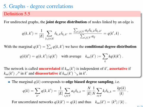
5. Graphs - degree correlationsDefinition 5.5
For undirected graphs, the joint degree distribution of nodes linked by an edge is
q(k, k′) =1|E|
∑(i,j)∈E
δki,kδkj,k′ =
∑i,j∈V aijδki,kδkj,k′∑
i,j∈V aij= q(k′, k) .
With the marginal q(k′) =∑
k q(k, k′) we have the conditional degree distribution
q(k|k′) = q(k, k′)/q(k′) with average knn(k′) :=∑
k
kq(k|k′) .
The network is called uncorrelated if knn(k′) is independent of k′, assortative ifknn(k′) in k′ and disassortative if knn(k′) in k′.
The marginal q(k) corresponds to edge biased degree sampling, i.e.
q(k) =∑
k′q(k, k′) =
1|E|∑i,j∈V
aijδki,k =N|E|
1N
∑i∈V
kiδki,k =kp(k)
〈k〉.
For uncorrelated networks q(k|k′) = q(k) and thus knn(k′) = 〈k2〉/〈k〉 .61 / 78
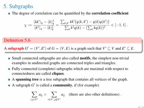
5. SubgraphsThe degree of correlation can be quantified by the correlation coefficient
χ :=〈kk′〉q − 〈k〉2q〈k2〉q − 〈k〉2q
=
∑k,k′ kk′
(q(k, k′)− q(k)q(k′)
)∑k k2q(k)− (
∑k kq(k))2 ∈ [−1, 1] .
Definition 5.6
A subgraph G′ = (V ′,E′) of G = (V,E) is a graph such that V ′ ⊆ V and E′ ⊆ E.
Small connected subgraphs are also called motifs, the simplest non-trivialexamples in undirected graphs are connected triples and triangles.Fully connected (complete) subgraphs which are maximal with respect toconnectedness are called cliques.A spanning tree is a tree subgraph that contains all vertices of the graph.A subgraph G′ is called a community, if (for example)∑
i,j∈V′aij >
∑i∈V′,j 6∈V′
aij (there are also other definitions) .
62 / 78
5. ClusteringClustering aims to quantify the probability that two neighbours of a given vertex arethemselves neighbours. Two different definitions are used in the literature.
Definition 5.7
The global clustering coefficient for an undirected graph is defined as
C =3× # of (connected) triangles
# of (connected) triples=
3∑
i<j<l aijajlali∑i<j<l(aijail + ajiajl + alialj)
∈ [0, 1] .
Alternatively, one can define a local clustering coefficient
Ci =# of triangles containing vertex i# of triples centered on vertex i
=
∑j<l aijajlali∑
j<l aijail∈ [0, 1] ,
and use the average 〈Ci〉 = 1N
∑i Ci to quantify clustering.
For a tree we have C = 〈Ci〉 = 0 and for the complete graph C = 〈Ci〉 = 1 .Higher-order clustering coefficients can be defined similarly, using differentsubgraphs as basis.
63 / 78
5. Graph spectraDefinition 5.8
The spectral density of a graph G = (V,E) is
ρ(λ) := 1N
∑i∈V δ(λ− λi) where λ1, . . . , λN ∈ C
are the eigenvalues of the adjacency matrix A.
Perron-Frobenius: A has a real eigenvalue λ1 > 0 with maximal modulus andreal, non-negative eigenvector(s). If the graph is connected, it has multiplicity 1and |λj| < λ1 for all other eigenvalues with j 6= 1.For undirected graphs, (An)ij is equal to the number of walks (paths whichallow repeated vertices) from i to j of length n. We also have
Tr(An) =∑N
i=1 λni and
(Tr(A)
)n= 0 ,
which can be used to derive statements like:∑i<j
λiλj = −|E| ,∑
i<j<l
λiλjλl = 2 ·# of triangles in G .
64 / 78
5. Graph LaplacianDefinition 5.9
The Graph Laplacian for a graph (V,E) with adjacency matrix A is defined as
Q := A− D where D =(δij
∑l 6=i
ail : i, j ∈ V).
Q has eigenvalues in C with real part Re(λ) < 0 except for λ1 = 0, whichfollows directly from the Gershgorin theorem and vanishing row sums.The multiplicity of λ1 equals the number of connected components inundirected graphs. Properly chosen orthogonal eigenvectors to λ1 have non-zeroentries on the individual connected components.The smaller the second largest real part of an eigenvalue, the harder it is to cut Ginto separated components by removing edges.Q defines a generator matrix of a continuous-time random walk on V withtransition rates aij. Using weighted graphs, any finite state CTMC can berepresented in this way.The Laplacian determines the first order linearized dynamics of many complexprocesses on graphs and is therefore of particular importance.
65 / 78
5. The Wigner semi-circle lawTheorem 5.1 (Wigner semi-circle law)
Let A = (aij : i, j = 1, . . . ,N) be a real, symmetric matrix with iid entries aij for i ≤ jwith finite moments, and E[aij] = 0, var[aij] = σ2 (called a Wigner matrix). Then thespectral density ρN of the matrix A/
√N converges in distribution to
ρN(λ)→ ρsc(λ) :=
(2πσ2)−1
√4σ2 − λ2 , if |λ| < 2σ
0 , otherwise.
The bulk of eigenvalues of unscaled Wigner matrices typically lies in the interval[−2√
Nσ, 2√
Nσ].Adjacency matrices A of GN,p random graphs are symmetric with iid Be(p)entries with E[aij] = p and var[aij] = p(1− p), so are not Wigner matrices.A has a maximal Perron-Frobenius eigenvalue of order pN, but all othereigenvalues have modulus of order
√N.
For fixed p > 0 or scaled p = pN pc = 1/N the Wigner semi-cirlce law holdsfor N →∞ with support width 4
√NσN .
For p = pN pc = 1/N the asymptotic spectral density deviates from ρsc.There is a related circular law for non-symmetric Wigner matrices.
66 / 78
5. More general graphs and networks
For multigraphs, multiple edges between nodes and loops (aii > 0) are allowed.Hypergraphs (V,E) are generalizations in which an edge can connect anynumber of vertices. Formally, the set of hyperedges E ⊆ P(V) is a set ofnon-empty subsets of V .In bipartite graphs the edge set can be partitioned into two sets V1,V2 ⊆ V eachnon-empty, with no connections within themselves, i.e. aij = aji = 0 for alli, j ∈ V1 and also for all i, j ∈ V2.Simple undirected examples include regular lattices Zd for d ≥ 1 which arepartitioned into sites with even and odd parity. Feed-forward neural networks areexamples of directed graphs with bipartite or multi-partite structure.Multilayer networks M = (G,C) consist of a family of m (weighted orunweighted) graphs Gα = (Vα,Eα) (called layers of M), and the set ofinterconnections between nodes of different layers
C =
cα,β ⊆ Vα × Vβ : α, β ∈ 1, . . . ,m, α 6= β.
Real examples include transportation networks or social networks with differenttypes of connections.
67 / 78
6. E-R Random graphs
Definition 6.1
An (Erdos-Renyi, short E-R) random graph G ∼ GN,K has uniform distribution onthe set of all undirected graphs with N vertices and K = |E|/2 edges, i.e.
PN,k[G = (V,E)] = 1/(N(N − 1)/2
K
).
An (E-R) random graph G ∼ GN,p has N vertices and each (undirected) edge ispresent independently with probability p ∈ [0, 1], i.e.
PN,p[G = (V,E)] = p|E|/2(1− p)N(N−1)/2−|E|/2 .
The ensemble GN,p is easier to work with and is mostly used in practice, and forN,K large, GN,K is largely equivalent to GN,p with p = 2K/(N(N − 1)).Since edges are present independently, graphs G ∈ GN,p should typically beuncorrelated. Indeed, one can show that χ(G), E[χ]→ 0 as N →∞.
68 / 78
6. E-R Random graphs - propertiesThe number of undirected edges for G ∼ GN,p is random, K ∼ Bi
(N(N−1)2 , p
).
For all i by homogeneity, ki ∼ Bi(N − 1, p) and E[〈k〉] = E[ki] = (N−1)p.The expected number of triangles in a GN,p graph is
(N3
)p3 ,
and the number of triples is(N
3
)3p2 .
Since fluctuations are of lower order, this implies for all GN ∼ GN,p
C(GN) =3(N
3
)p3(1 + o(1))(N
3
)3p2(1 + o(1))
→ p as N →∞ .
The expected degree distribution for GN ∼ GN,p is Bi(N − 1, p). In the limitN →∞ with p = pN = z/(N − 1) keeping z = E[〈k〉] fixed we have
E[p(k)] = P[ki = k] =
(N − 1
k
)pk
N(1− pN)N−1−k → zk
k!e−z .
Therefore, E-R GN,p graphs are sometimes called Poisson random graphs.In this scaling limit E-R graphs are locally tree-like, i.e. connected components
Cni := j ∈ V : j↔ i, dij ≤ n , n fixed
are tree subgraphs as N →∞ with probability 1.Vertex degrees are ki ∼ Poi(z) and iid kj ∼ Poi(z) + 1.
69 / 78
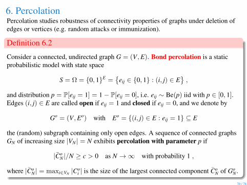
6. PercolationPercolation studies robustness of connectivity properties of graphs under deletion ofedges or vertices (e.g. random attacks or immunization).
Definition 6.2
Consider a connected, undirected graph G = (V,E). Bond percolation is a staticprobabilistic model with state space
S = Ω = 0, 1E =
eij ∈ 0, 1 : (i, j) ∈ E,
and distribution p = P[eij = 1] = 1− P[eij = 0], i.e. eij ∼ Be(p) iid with p ∈ [0, 1].Edges (i, j) ∈ E are called open if eij = 1 and closed if eij = 0, and we denote by
Go = (V,Eo) with Eo = (i, j) ∈ E : eij = 1 ⊆ E
the (random) subgraph containing only open edges. A sequence of connected graphsGN of increasing size |VN | = N exhibits percolation with parameter p if
|CoN |/N ≥ c > 0 as N →∞ with probability 1 ,
where |CoN | = maxi∈VN |Co
i | is the size of the largest connected component CoN of Go
N .
70 / 78
6. Percolation and E-R graphsAlternatively, percolation can be defined on an infinite graph G (e.g. Zd) with
percolation probability θ(p) = P[|C0| =∞]
= 0 , for p < pc
> 0 , for p > pc,
changing behaviour at a critical value pc ∈ [0, 1].In site percolation vertices and their adjacent edges are deleted.E-R random graphs GN,p have the same distribution as open subgraphs(Go,Eo) ⊆ KN under percolation on the complete graph KN with parameter p.
Theorem 6.1 (Giant component for E-R graphs)
Consider GN,p ∼ GN,p with p = z/N and maximal connected component CN,p. Then
|CN,p| =
O(log N) , for z < 1O(N2/3) , for z = 1
O(N) , for z > 1and θ(z) =
0 , for z ≤ 1> 0 , for z > 1→ 1 , for z→∞
where θ(z) := limN→∞ |CN,p|/N is a continuous, monotone increasing function of z.For z > 1, CN,p is the only giant component, and the second largest is O(log N).
Local trees with 1 + Poi(z) degrees die out with probability 1 if and only if z ≤ 1.71 / 78
6. Preferential attachmentThe prevalence of power-law degree distributions in real complex networks can beattributed to growth mechanisms subject to preferential attachment.
Definition 6.3
Starting with a complete graph (V0,E0) of |V0| = m0 nodes, at each time stept = 1, . . . ,N − m0 a new node j = t + m0 is added. It forms m ≤ m0 undirected edgeswith existing nodes i ∈ Vt−1 with a probability proportional to their degreeπj↔i = ki/
∑l∈Vt
kl (preferential attachment).The resulting, undirected graph with N nodes and K = m0(m0 − 1)/2 + m(N −m0) iscalled a Barabasi-Albert random graph, denoted by GBA
N,K .
As N →∞, the average degree is 〈k〉 = 2m and the degree distribution pN(k)converges to a distribution p(k) with power law tail, i.e. p(k) = Ck−α for largek where α = 3, which is close to exponents observed for real-world networks.This is independent of the parameters m0 and m.Characteristic path length and clustering coefficient typically behave likeL = O(log N) and C = O(N−0.75) for GBA
N,K graphs, and they are uncorrelated.They are not homogeneous, the expected degree of nodes increases with age.
72 / 78
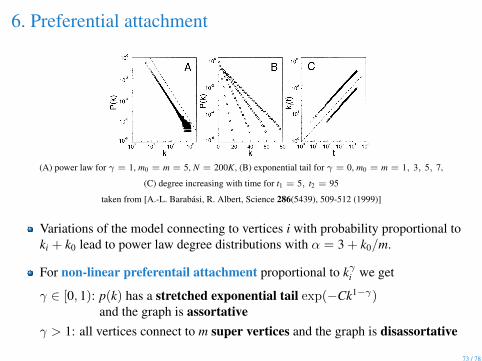
6. Preferential attachment
(A) power law for γ = 1, m0 = m = 5, N = 200K, (B) exponential tail for γ = 0, m0 = m = 1, 3, 5, 7,
(C) degree increasing with time for t1 = 5, t2 = 95
taken from [A.-L. Barabasi, R. Albert, Science 286(5439), 509-512 (1999)]
Variations of the model connecting to vertices i with probability proportional toki + k0 lead to power law degree distributions with α = 3 + k0/m.
For non-linear preferentail attachment proportional to kγi we get
γ ∈ [0, 1): p(k) has a stretched exponential tail exp(−Ck1−γ)and the graph is assortative
γ > 1: all vertices connect to m super vertices and the graph is disassortative
73 / 78
6. Small-world networksDefinition 6.4
A sequence of connected graphs GN with increasing size |VN | = N exhibits thesmall-world property, if the characteristic path length L(GN) = O(log N).
Examples include trees with degrees ki ≥ 3 and also the giant or largest component inE-R random graphs. In most graph models small-worldness is paired with lowclustering coefficients, e.g. 0 for trees and p for GN,p graphs. However, many realexamples of small world networks exhibit also large clustering coefficients, such asnetworks of social contacts.
Definition 6.5
Consider a 2m-regular ring graph with adjacency matrix aij =
1 , |i− j| ≤ m0 , otherwise
of size N with a total number of K = mN undirected edges.For all i, each edge (i, j) with a clockwise neighbour with j > i is rewired withprobability p ∈ [0, 1], i.e. replaced by an edge (i, l) where l is chosen uniformlyamong vertices not adjacent to i. The resulting graph is a Watts-Strogatz randomgraph, denoted by GWS
N,K .
74 / 78
6. Watts-Strogatz model
W-S random graphs interpolate between a regular lattice for p = 0 and a GN,K
E-R random graph conditioned on the event that all vertices have degree ki ≥ m.Expected clustering coefficient E[C(p)] and characteristic path length E[L(p)]are monotone decreasing functions of p and show the following behaviour.
N = 1000 and m = 5, taken from [D.J. Watts, S.H. Strogatz, Nature 393, 440-442 (1998)]
75 / 78
6. Configuration model
Definition 6.6
The configuration model GconfN,D is defined as the uniform distribution among all
undirected graphs with N vertices with a given degree sequence D = (k1, . . . , kN),such that
∑i∈V ki = 2K.
Not all sequences D that sum to an even number are graphical.Sampling is usually done by attaching ki half edges to each vertex i and matchingthem randomly. This can lead to self loops and rejections.General randomized graphs with given degree distribution p(k) can be sampledin the same way. If kmax = maxi ki is bounded, one can show that these graphsexhibit a giant (connected) component of size O(N) if
Q :=∑
k≥0 k(k − 2)p(k) > 0 ,
and if Q < 0 the largest component is of size O(k2max log N).
For directed versions with Din and Dout we need∑
i∈V kini =
∑i∈V kout
i .
76 / 78
6. Planar graphs and spatial point processesDefinition 6.7
A planar graph is an undirected graph that can be embedded in the plane, i.e. it canbe drawn in such a way that no edges cross each other. The edges of a particularembedding partition the plane into faces. A connected planar graph G has a dualgraph G∗, which has one vertex in each face of G, and a unique edge crossing eachedge of G. G∗ may be a multigraph with self-loops.A maximal planar graph is called a triangulation.
Every planar graph is 4-partite or 4-colourable.In a triangulation each face is bounded by three edges. By induction, everytriangulation with N>2 nodes has K=3N−6 undirected edges and 2N−4 faces.
Definition 6.8
A random countable set Π ⊆ Rd is called a spatial point process.Π ⊆ Rd is called a homogeneous Poisson point process PPP(λ) with rate λ > 0 if
for all A ⊆ Rd we have N(A) := |Π ∩ A| ∼ Poi(λ|A|) ,for all disjoint A1, . . . ,An ⊆ Rd, N(A1), . . . ,N(An) are independent.
77 / 78
6. Planar graphs and spatial point processesTo sample from a PPP(λ) e.g. in a box A = [0,L]d, pick N(A) ∼ Poi(λLd), thenplace N(A) particles independently in A each with uniform distribution, i.e. pickthe d coordinates uniformly in [0,L].A Poisson process PP(λ) is equivalent to a PPP(λ) on [0,∞).
Definition 6.9
Let Π = x1, x2, . . . be a countable subset of Rd, endowed with a distance functiond(x, y). A Voronoi tesselation (or diagram) is given by the family of Voronoi cellsA1,A2, . . . ⊆ Rd where
Ai =
x ∈ Rd : d(x, xi) ≤ d(x, xj) for all j 6= i
is the set of points closest to xi.
Properties in 2 dimensions.The shape of Voronoi cells depends on the distance function, for Euclideandistance d(x, y) =
√(x1 − y1)2 + (x2 − y2)2 they are convex polygons, and
boundaries between adjacent cells are straight lines.The dual graph of a Voronoi diagram of a set Π is called Delaunaytriangulation, which is not unique if 4 or more cells intersect in a point.