The Rockefeller University Press $30.00J. Cell Biol. Vol. 216 No. 1 65–71https://doi.org/10.1083/jcb.201610026
IntroductionMicroscopy assays enable the identification of cell biologi-cal phenotypes through the quantification of cell morphology. These image-based methods are often used in genetically or environmentally sensitized conditions to probe the relationship between cell structure and function in response to a perturbation of interest (Liberali et al., 2015). For example, many groups have used light microscopy to investigate the phenotypic conse-quences of single-gene knockouts on cell morphology (Turner et al., 2012). By integrating fluorescently labeled proteins or staining specific organelles, it is possible to investigate more complex subcellular phenotypes (Boutros et al., 2004; Negishi et al., 2009). Image-based assays of cellular and subcellular phenotypes have been performed in a variety of organisms and cell lines probing numerous cell biological processes, rang-ing from the effects of chemical treatments on protein subcel-lular localization in yeast (Chong et al., 2015) to the genetic contributors of more complex phenotypes such as the mitotic exit program in human cell lines (Schmitz et al., 2010; Matti-azzi Usaj et al., 2016).
Technological advancements have led to the develop-ment of automated fluorescent confocal microscopes that in-crease throughput, enabling thousands of images to be acquired in a single day. This increase in data production has resulted in a new demand for efficient, automated computational im-age-analysis strategies to overcome the resultant bottleneck
associated with manual data scoring. Perhaps more importantly, computational analyses also enable identification and quanti-fication of subtle phenotypes that would otherwise be impos-sible to score manually.
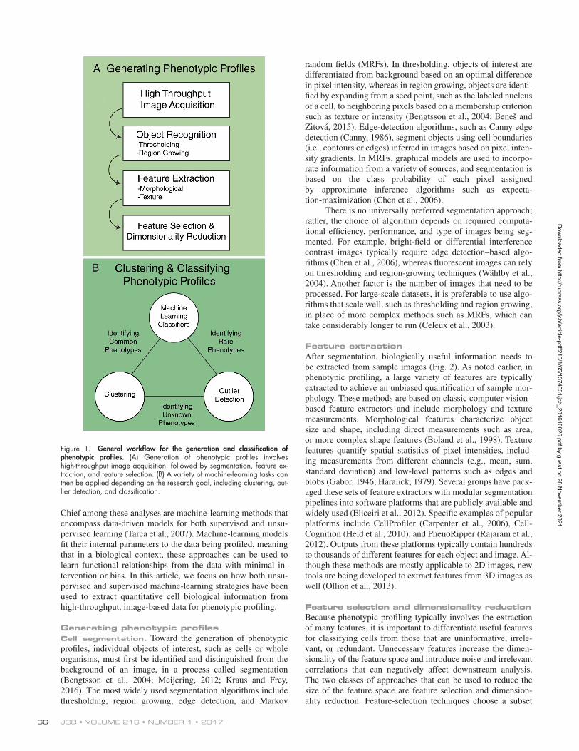
Although there is no single solution for computational analysis of biological images, most image analysis pipelines follow a common workflow in which individual cells are iden-tified as unique objects, from which phenotypic measurements, or features, are extracted from these single cells. These quanti-tative features typically include measures of cell shape and size, pixel intensity, and texture. Depending on the research goal, the features can then be clustered or classified in a variety of dif-ferent ways to enable an unbiased assessment of phenotypes of interest (Fig. 1). For classification or clustering, single-cell data from an individual experiment or treatment are typically aggre-gated in a manner that reflects distributions within populations.
Several different groups have used this general imaging platform in a targeted approach to quantify a single process or cellular function, which is often referred to as phenotypic screening. During the analysis of screening data, specific features relevant to the phenotype of interest are considered (Caicedo et al., 2016). For example, in a screen designed to identify cell size mutants, size-based image features will be identified and used to discriminate populations of cells that are unusually small or large relative to a wild-type size distribu-tion (Kitami et al., 2012). Many of the studies published using high-throughput microscopy have used this targeted approach, considering one or two single-cell features in their analysis (Singh et al., 2014). Alternatively, phenotypic profiling involves a less targeted approach in which many features of the sam-ple are quantified, allowing for the identification of as many properties of the sample as possible and enabling the features that describe these properties to differentiate samples from one another in an unbiased manner (Caicedo et al., 2016). For example, in a high-throughput chemical screening project in which cell samples are exposed to an array of small molecules, changes in cell morphology can be quantified and used to infer a mechanism of drug action in downstream experiments (Perlman et al., 2004; Ljosa et al., 2013).
Given this unbiased approach to phenotypic profiling, multiple analysis strategies allow researchers to translate mor-phological features into meaningful biological information.
With recent advances in high-throughput, automated mi-croscopy, there has been an increased demand for effec-tive computational strategies to analyze large-scale, image-based data. To this end, computer vision ap-proaches have been applied to cell segmentation and fea-ture extraction, whereas machine-learning approaches have been developed to aid in phenotypic classification and clustering of data acquired from biological images. Here, we provide an overview of the commonly used com-puter vision and machine-learning methods for generat-ing and categorizing phenotypic profiles, highlighting the general biological utility of each approach.
Machine learning and computer vision approaches for phenotypic profiling
Ben T. Grys,1,2 Dara S. Lo,1,2 Nil Sahin,1,2 Oren Z. Kraus,2,3 Quaid Morris,1,2,3 Charles Boone,1,2 and Brenda J. Andrews1,2
1Department of Molecular Genetics and 2Terrence Donnelly Centre for Cellular and Biomolecular Research, University of Toronto, Toronto, Ontario M5S 3E1, Canada3Department of Electrical and Computer Engineering, University of Toronto, Toronto, Ontario M5S 2E4, Canada
Correspondence to Charles Boone: [email protected]; or Brenda J. Andrews: [email protected] used: MRF, Markov random field; RF, random forest; SVM, support vector machine.
TH
EJ
OU
RN
AL
OF
CE
LL
BIO
LO
GY
Dow
nloaded from http://rupress.org/jcb/article-pdf/216/1/65/1374031/jcb_201610026.pdf by guest on 28 N
Chief among these analyses are machine-learning methods that encompass data-driven models for both supervised and unsu-pervised learning (Tarca et al., 2007). Machine-learning models fit their internal parameters to the data being profiled, meaning that in a biological context, these approaches can be used to learn functional relationships from the data with minimal in-tervention or bias. In this article, we focus on how both unsu-pervised and supervised machine-learning strategies have been used to extract quantitative cell biological information from high-throughput, image-based data for phenotypic profiling.
Generating phenotypic profilesCell segmentation. Toward the generation of phenotypic profiles, individual objects of interest, such as cells or whole organisms, must first be identified and distinguished from the background of an image, in a process called segmentation (Bengtsson et al., 2004; Meijering, 2012; Kraus and Frey, 2016). The most widely used segmentation algorithms include thresholding, region growing, edge detection, and Markov
random fields (MRFs). In thresholding, objects of interest are differentiated from background based on an optimal difference in pixel intensity, whereas in region growing, objects are identi-fied by expanding from a seed point, such as the labeled nucleus of a cell, to neighboring pixels based on a membership criterion such as texture or intensity (Bengtsson et al., 2004; Beneš and Zitová, 2015). Edge-detection algorithms, such as Canny edge detection (Canny, 1986), segment objects using cell boundaries (i.e., contours or edges) inferred in images based on pixel inten-sity gradients. In MRFs, graphical models are used to incorpo-rate information from a variety of sources, and segmentation is based on the class probability of each pixel assigned by approximate inference algorithms such as expecta-tion-maximization (Chen et al., 2006).
There is no universally preferred segmentation approach; rather, the choice of algorithm depends on required computa-tional efficiency, performance, and type of images being seg-mented. For example, bright-field or differential interference contrast images typically require edge detection–based algo-rithms (Chen et al., 2006), whereas fluorescent images can rely on thresholding and region-growing techniques (Wählby et al., 2004). Another factor is the number of images that need to be processed. For large-scale datasets, it is preferable to use algo-rithms that scale well, such as thresholding and region growing, in place of more complex methods such as MRFs, which can take considerably longer to run (Celeux et al., 2003).
Feature extractionAfter segmentation, biologically useful information needs to be extracted from sample images (Fig. 2). As noted earlier, in phenotypic profiling, a large variety of features are typically extracted to achieve an unbiased quantification of sample mor-phology. These methods are based on classic computer vision–based feature extractors and include morphology and texture measurements. Morphological features characterize object size and shape, including direct measurements such as area, or more complex shape features (Boland et al., 1998). Texture features quantify spatial statistics of pixel intensities, includ-ing measurements from different channels (e.g., mean, sum, standard deviation) and low-level patterns such as edges and blobs (Gabor, 1946; Haralick, 1979). Several groups have pack-aged these sets of feature extractors with modular segmentation pipelines into software platforms that are publicly available and widely used (Eliceiri et al., 2012). Specific examples of popular platforms include CellProfiler (Carpenter et al., 2006), Cell-Cognition (Held et al., 2010), and PhenoRipper (Rajaram et al., 2012). Outputs from these platforms typically contain hundreds to thousands of different features for each object and image. Al-though these methods are mostly applicable to 2D images, new tools are being developed to extract features from 3D images as well (Ollion et al., 2013).
Feature selection and dimensionality reductionBecause phenotypic profiling typically involves the extraction of many features, it is important to differentiate useful features for classifying cells from those that are uninformative, irrele-vant, or redundant. Unnecessary features increase the dimen-sionality of the feature space and introduce noise and irrelevant correlations that can negatively affect downstream analysis. The two classes of approaches that can be used to reduce the size of the feature space are feature selection and dimension-ality reduction. Feature-selection techniques choose a subset
Figure 1. General workflow for the generation and classification of phenotypic profiles. (A) Generation of phenotypic profiles involves high-throughput image acquisition, followed by segmentation, feature ex-traction, and feature selection. (B) A variety of machine-learning tasks can then be applied depending on the research goal, including clustering, out-lier detection, and classification.
Dow
nloaded from http://rupress.org/jcb/article-pdf/216/1/65/1374031/jcb_201610026.pdf by guest on 28 N
ovember 2021
machine learning for phenotypic profiling • Grys et al. 67
of features from the original feature space that are determined to be most relevant to the machine-learning task (Saeys et al., 2007). For example, Loo et al. (2007) selected a subset of in-formative features by iteratively removing other subsets that did not affect downstream performance of their classifier. In con-trast, dimensionality-reduction techniques transform the orig-inal feature space into lower dimensions using linear methods (such as principal components analysis [PCA]) or nonlinear techniques (such as t-distributed stochastic neighbor embed-ding; Van Der Maaten and Hinton, 2008) that preserve the vari-ance in the dataset. The selected or transformed set of features can then be treated as a single vector representing the pheno-typic profile of a given sample.
Dimensionality-reduction algorithms can be fitted di-rectly to most datasets and automatically provide reduced feature representations. In contrast, feature-selection methods require more effort and domain expertise to implement. How-ever, a significant benefit of feature selection is that the original features are maintained, thereby preserving the interpretability of the features used in downstream models.
Clustering and classifying phenotypic profilesAfter selecting the features that best represent the phenotypic information in a dataset, a variety of computational strategies can be used to cluster or classify the resultant profiles into bio-logically interpretable groups. The choice of approach is largely dependent on the distribution of distinct phenotypes repre-sented in the dataset as well as any prior knowledge of what those phenotypes might be.
In machine-learning terminology, clustering is a form of unsupervised learning in which models are trained using an un-labeled dataset and patterns are discovered by grouping similar data points. In contrast, classification is a form of supervised learning in which models are trained on labeled datasets to gen-erate predictions on unseen data points (Libbrecht and Noble, 2015). Choosing whether to use unsupervised or supervised learning ultimately depends on how well defined classes of
phenotypes are a priori, as well as how many training examples can be identified for each phenotypic category. A third approach is outlier detection, in which normal or wild-type phenotypes are known and the goal is to find examples of rare phenotypes that differ significantly from the reference samples. Here we re-view clustering, outlier detection, and classification approaches.
Clustering. Clustering is typically the simplest ap-proach for grouping phenotypic profiles into biologically inter-pretable classes and is appropriate when the desired or expected output of classification is not known (Fig. 3 A). For example, Young et al. (2008) profiled a library of ∼6,500 compounds for cell cycle defects in HeLa cells. In that study, hierarchical clus-tering of the profiles generated from imaging of the top ∼200 most responsive compounds identified seven phenotypic cate-gories. The cell cycle defects represented in those clusters cor-responded with compound structure similarity, suggesting that the clusters were driven by related molecules that share a com-mon biological target. Clustering was an ideal approach for classifying and interpreting these data, because the dataset in-cluded a variety of complex phenotypes, and no knowledge of the phenotypes was required before classification. Furthermore, had the researchers assumed a specific phenotypic output, some significant classes may have been overlooked or misclassified, exemplifying the importance of the unsupervised approach. For this reason, hierarchical clustering has been implemented by many groups in several different organisms (Bakal et al., 2007; Seewald et al., 2010; Gustafsdottir et al., 2013; Handfield et al., 2013) and is often the first approach used if there is any uncer-tainty regarding the expected phenotypic output.
Outlier detection. Although clustering is an ideal un-supervised approach for classification of common phenotypes, it may fail to identify rare profiles within a dataset. For exam-ple, if a particular phenotype is present at a low frequency, pro-files representing that phenotype will likely get grouped into a similar, yet biologically distinct, cluster; this may cause rare profiles to be misclassified and their underlying biology to be misinterpreted or overlooked by the researcher.
Figure 2. Micrographs of individual budding yeast cells identified during segmentation, with illustrative examples of four types of features that could be identified during feature extraction. In these micrographs, red pixels mark the cellular cytosol, whereas green pixels represent GFP-fusion proteins that localize to unique subcellular structures in each cell. Area features are concerned with the number of pixels in the segmented region, GFP intensity features consider overall green pixel brightness, shape features examine the contours of the cell objects, and texture examines the spatial arrangement of pixel intensities. These features, and many others, are quantified for each cellular object and then used in downstream clustering or classification.
Dow
nloaded from http://rupress.org/jcb/article-pdf/216/1/65/1374031/jcb_201610026.pdf by guest on 28 N
ovember 2021
JCB • Volume 216 • NumBer 1 • 201768
Outlier detection seeks to identify profiles that are highly dissimilar from the remaining data (Knorr and Ng, 1998; Hodge and Austin, 2004; Fig. 3 B). Many different algorithms exist for performing outlier detection based on statistics (Barnett and Lewis, 1994), distance (Knorr and Ng, 1998; Ramaswamy et al., 2000), density (Breunig et al., 2000), clustering (Jain et al., 1999; He et al., 2003), and deviation (Arning et al., 1996). One of the most commonly used methods is density-based outlier de-tection, which identifies outliers based on an object’s neighbor-hood density (Breunig et al., 2000). The power of density-based methods is that they provide improved performance relative to methods that use statistical or computational geometry princi-ples, but they suffer from an inability to scale well (Orair et al., 2010). A second commonly used approach is distance-based outlier detection, which is based on the k-nearest neighbor al-gorithm (Knorr and Ng, 1998) and uses a well-defined distance metric (e.g., Euclidean, Mahalanobis) to determine outliers (Ramaswamy et al., 2000). Put simply, the greater the distance of the profile from its neighbors, the more likely it is to be an outlier. The power of distance-based outlier detection lies in its simplicity and scalability to large datasets with high dimension-ality (Orair et al., 2010). However, outlier detection identifies images that are very different from other images, and these outliers must be manually inspected to assign them biological significance. This process may allow for the detection of rare phenotypes that are difficult to detect with other methods.
Although outlier detection algorithms have been widely used in fraud detection and equipment monitoring, as well as for removal of biological noise, they have been less developed for high-dimensional data such as images (Ju et al., 2015; Li et al., 2015). One important biological application of outlier detection is in biomedical image analysis. For example, a statistical-based outlier detection method was used to provide reliable and fully automated quantitative diagnosis of white-matter hypersensitiv-ities in the brains of elderly subjects (Caligiuri et al., 2015).
Classification. Although clustering and outlier detec-tion are powerful unsupervised methods for phenotypic profile classification, they both require substantial evaluation and vali-dation of the identified categories to enable cogent biological interpretation. Alternatively, supervised methods necessitate that phenotypic categories are established before classification, making evaluation and validation of classes much easier. Clas-sification is one of the most commonly used approaches for phenotypic analysis of image-based data. Broadly, classifiers
are preassigned a distinct set of categorical class outputs (sub-cellular localization classes, mutant compartment morphology classes, etc.), and the classifier is then trained to recognize fea-ture profiles that are representative of each class, such that novel profiles can be classified into one or more discrete output classes based on feature similarity to the training data (Libbrecht and Noble, 2015). Next we review the two major types of classifiers, linear and nonlinear models.
Linear classifiers. Linear classifiers combine input features in a linear combination and then assign classification based on the output value. As such, linear classifiers define a decision boundary, called a hyperplane, that separates the classes in the dataset (illustrated for a 2D example in Fig. 3 C). Several types of linear classifiers have been used to analyze im-age-based data. For example, naive Bayes is a linear classifica-tion model that uses Bayes theorem to analyze feature probabilities and assumes feature independence. This approach is particularly useful when the dataset is large and contains many different features. Jolly et al. (2016) recently applied a naive Bayes classifier to images generated from a genome-wide RNAi screen of lysosome motility in the Drosophila melano-gaster S2 model cell system. Images were classified from more than 17,000 gene knockdowns, and samples with an abnormal degree of lysosomal motility were identified with 94% accu-racy. A similar model that assumes equal covariance among the classes is Fisher’s linear discriminant (Wang et al., 2008). This approach assigns weights to each feature in the dataset, high-lighting features that have high variance in the data and may be more useful for classification. This model was recently applied to the study of neuronal differentiation in PC12 cells (Weber et al., 2013) and has been used to classify a diverse range of image-based datasets (Wang et al., 2008; Horn et al., 2011; Pardo-Martin et al., 2013). Fisher’s method performs best for low-dimensional, small datasets, whereas the combination of PCA and naive Bayes can provide a performance similar to Fisher’s method when applied to large datasets.
A second major group of linear classifiers directly model decision boundaries. In other words, these models directly predict class membership given features, without modeling the joint probabilities of classes and features (Ng and Jordan, 2002). A common example is a linear support vector machine (SVM), which defines a hyperplane that separates two classes by maximizing the distance between the hyperplane and the data points from opposite classes closest to each other (called
Figure 3. Schematic representation of unsupervised and supervised methods to classify phenotypic profiles. (A–D) Each shape represents one object in the dataset. All features associated with each object are reduced to 2D feature space. D
ownloaded from
http://rupress.org/jcb/article-pdf/216/1/65/1374031/jcb_201610026.pdf by guest on 28 Novem
ber 2021
machine learning for phenotypic profiling • Grys et al. 69
support vectors; Noble, 2006). This hyperplane is generated based on images of manually annotated samples, and the SVM classifier assigns membership to new data points based on their positions relative to the hyperplane (Weston et al., 2000).
Chong et al. (2015) recently generated an ensemble of ∼60 binary linear SVM classifiers to assign GFP-fusion proteins in images of budding yeast cells to 16 distinct subcellular com-partments. Classification accuracy was compartment specific, but on average, the SVM classifier ensemble performed with >70% precision and recall. SVM classifiers were useful for an-alyzing this set of protein subcellular localization data, largely because of the high quality of the training set. In this case, the training set was composed of high-quality ground-truth exam-ples of GFP-fusion proteins localized to distinct compartments and reported in the abundance of literature on manually scored protein localizations in budding yeast.
Nonlinear classifiers. Nonlinear classification algo-rithms are required when the decision boundary is nonlinear and potentially discontinuous (Fig. 3 D). These algorithms are more complex than linear classifiers and generally require more training data to fit. For example, the SVM classifiers described earlier can be used to produce nonlinear decision boundaries if nonlinear kernel functions are used. These functions transform the feature space before fitting the SVM model for classifica-tion, enabling nonlinear decision boundaries in the original fea-ture space (Weston et al., 2000). Nonlinear SVM classifiers have been used to distinguish aberrant HeLa cell morphology after RNAi-mediated gene knockdown (Fuchs et al., 2010). In that study, cells were classified into one of 10 distinct morpho-logical classes, including groups for elongated, enlarged, or condensed morphologies as well as cell cycle arrest phenotypes. Numerous other groups have also taken advantage of SVM classifiers to classify morphological phenotypes in human cells, including mutant morphology (Schmitz et al., 2010), cell cycle arrest phenotypes (Neumann et al., 2010), and subcellular local-ization classes (Conrad et al., 2004).
Another example of a nonlinear classification algorithm is a random forest (RF) classifier. The underlying principle of an RF classifier is to use a series of decision/classification trees that map the features of a sample to a class output. These are referred to as classification trees because of their branch-like structure in which features are conjugated in a path such that a particular combination will trickle down to a resultant class output. RF classifiers combine an ensemble of uncorrelated decision trees with random feature combinations to reduce the variance in the data and help resolve issues with overfitting the data to the training set (Hastie et al., 2005). Roosing et al. (2015) performed an siRNA knockdown study of ∼18,000 genes in a human cell line to look for genes that might be implicated in cilia formation. After extracting and selecting 18 nonoverlap-ping cellular features, an RF classifier was trained on positive (aberrant cilia) and negative (wild-type cilia) instances.
Considerations. Validation and testing are both im-portant steps that must be performed on separate datasets to en-sure that a classifier can generalize to new datasets. Classifiers update their internal parameters during the training phase in a manner that reduces the error rates between predicted values and the given labels on the training set. With many nonlinear classifiers (and some linear classifiers), these updates may con-tinue to the point where the model’s performance begins to de-teriorate on unseen validation data but continues to improve on the training set. This behavior is referred to as overfitting to the
training dataset. Overfitting becomes more severe as the model complexity (i.e., the number of trainable parameters in the model) increases relative to the size of the dataset. An approxi-mate guideline is that the number of data points in the training set should be a small multiple of the number of parameters in the model (∼5–10). An additional class of techniques that pre-vent complex models from overfitting to the training data are called model regularization. Regularization typically modifies the model training procedure in a manner that prevents the mod-el’s parameters from fitting to noise or specificities in the train-ing data. To evaluate whether models are overfitting, two separate datasets are typically held out and are used to ensure that models generalize to new datasets. The validation set is used to optimize the model, whereas the test set is a held-out dataset used only with the final implementation to compare dif-ferent classification approaches. For small datasets, an alterna-tive to held-out validation sets is k-fold cross validation, in which the model is repeatedly trained k times on k separate sub-sets of the available data and evaluated on the remaining data during each repetition. In the extreme case, this is called leave-one-out cross validation, in which the model is repeatedly trained by leaving out one data point and is then validated on the left-out data point. For both forms of cross validation, the mean of the validations across the repetitions is used as the valida-tion metric (Bishop, 2006).
The approaches we have described so far aim to profile individual cells, but researchers often need to summarize these findings on a per-sample or population basis. Various methods are used to aggregate single-cell profiles, including techniques that maintain information regarding subpopulation heteroge-neity. The most straightforward methods for aggregating sin-gle-cell profiles across treatment conditions include calculating statistics, such as the mean or median across the population, for each feature (Ljosa et al., 2013). When comparing conditions, statistical tests that include variance estimates, such as t tests and Z-factors, may be used (Singh et al., 2014). In addition, the Kolmogorov–Smirnov statistic is a popular metric, as it does not assume normal distribution of features (Perlman et al., 2004) and compares population distributions directly. Finally, pipelines that categorize individual cells based on clustering, classification, or small subsets of descriptive features can be used to study how the cell subpopulation proportions change under different conditions (Snijder et al., 2009).
PerspectiveTypically, research groups implement the classification ap-proach that works best for their particular dataset or that they are the most familiar with implementing. However, this strat-egy can lead to duplicated efforts, as new image sets often re-quire labeling new training sets for classification, even when classifying identical phenotypes seen in previous assays. This is largely because many of the classic machine-learning strat-egies described here fail to discover the intricate structure of large datasets, making it difficult to apply them to multiple as-says. This difficulty is partly a result of the feature extraction and dimensionality reduction steps, which typically vary for different assays. Recently, deep learning technologies have been developed that learn feature representations and classifi-cation boundaries directly from raw pixel data. In deep learn-ing, multilayer, nonlinear classifiers called neural networks use back-propagation during training to learn how the network should update its internal parameters to minimize classification
Dow
nloaded from http://rupress.org/jcb/article-pdf/216/1/65/1374031/jcb_201610026.pdf by guest on 28 N
ovember 2021
JCB • Volume 216 • NumBer 1 • 201770
error in each layer, ultimately discovering intricate hierarchical feature representations that can be broadly applied to multiple image sets (LeCun et al., 2015).
Based on this approach, deep learning networks have re-cently surpassed human-level accuracy at classifying modern object recognition benchmarks (Krizhevsky et al., 2012). Deep learning has been applied to numerous types of biological data for modeling gene expression (Chen et al., 2016a,b) and pre-dicting protein structure (Zhou and Troyanskaya, 2015), DNA methylation (Wang et al., 2016), and protein–nucleic acid in-teractions (Alipanahi et al., 2015). Deep learning has also been used to classify protein localization in yeast and mechanisms of action in a publicly available drug screen (Kraus et al., 2016; Pärnamaa and Parts, 2016 Preprint). Based on the success of deep learning, its application to biological image data should overcome the pitfalls associated with conventional analysis pipelines, with the potential to automate the entire process of de-veloping analysis pipelines for classifying cellular phenotypes.
Acknowledgments
The authors declare no competing financial interests.
Imaging work in the Andrews and Boone labs is supported by founda-tion grants from the Canadian Institutes of Health Research.
Submitted: 10 October 2016Revised: 18 November 2016Accepted: 21 November 2016
ReferencesAlipanahi, B., A. Delong, M.T. Weirauch, and B.J. Frey. 2015. Predicting the
sequence specificities of DNA- and RNA-binding proteins by deep learning. Nat. Biotechnol. 33:831–838. http ://dx .doi .org /10 .1038 /nbt .3300
Arning, A., R. Agrawal, and P. Raghavan. 1996. A linear method for deviation in large databases. In KDD ’96 Proceedings of the Second International Conference on Knowledge Discovery and Data Mining.E. Simoudis, J. Han, and U. Fayyad, editors. AAAI Press, Menlo Park, CA. 164–169.
Bakal, C., J. Aach, G. Church, and N. Perrimon. 2007. Quantitative morphological signatures define local signaling networks regulating cell morphology. Science. 316:1753–1756. http ://dx .doi .org /10 .1126 /science .1140324
Barnett, V., and T. Lewis. 1994. Outliers in statistical data. John Wiley and Sons, New York, NY.
Beneš, M., and B. Zitová. 2015. Performance evaluation of image segmentation algorithms on microscopic image data. J. Microsc. 257:65–85. http ://dx .doi .org /10 .1111 /jmi .12186
Bengtsson, E., C. Wählby, and J. Lindblad. 2004. Robust cell image segmentation methods. Pattern Recognit. Image Anal. 14:157–167. http ://dx .doi .org /10 .1017 /CBO9781107415324 .004
Bishop, C.M. 2006. Pattern Recognition and Machine Learning. Springer, New York, NY. 738 pp.
Boland, M.V., M.K. Markey, and R.F. Murphy. 1998. Automated recognition of patterns characteristic of subcellular structures in fluorescence microscopy images. Cytometry. 33:366–375. http ://dx .doi .org /10 .1002 /(SICI)1097 -0320(19981101)33 :3<366::AID-CYTO12>3.0.CO;2-R
Boutros, M., A.A. Kiger, S. Armknecht, K. Kerr, M. Hild, B. Koch, S.A. Haas, R. Paro, N. Perrimon, and Heidelberg Fly Array Consortium. 2004. Genome-wide RNAi analysis of growth and viability in Drosophila cells. Science. 303:832–835. http ://dx .doi .org /10 .1126 /science .1091266
Breunig, M.M., H.-P. Kriegel, R.T. Ng, and J. Sander. 2000. LOF: Identifying density-based local outliers. In SIG MOD ’00 Proceedings of the 2000 ACM SIG MOD International Conference on Management of Data.M. Dunham, J.F. Naughton, W. Chen, and N. Koudas, editors. ACM, New York, NY. 93–104. http ://dx .doi .org /10 .1145 /335191 .335388
Caicedo, J.C., S. Singh, and A.E. Carpenter. 2016. Applications in image-based profiling of perturbations. Curr. Opin. Biotechnol. 39:134–142. http ://dx .doi .org /10 .1016 /j .copbio .2016 .04 .003
Caligiuri, M.E., P. Perrotta, A. Augimeri, F. Rocca, A. Quattrone, and A. Cherubini. 2015. Automatic detection of white matter hyperintensities in healthy aging and pathology using magnetic resonance imaging: A review. Neuroinformatics. 13:261–276. http ://dx .doi .org /10 .1007 /s12021 -015 -9260 -y
Canny, J. 1986. A computational approach to edge detection. IEEE Trans. Pattern Anal. Mach. Intell. 8:679–698. http ://dx .doi .org /10 .1109 /TPA MI .1986 .4767851
Carpenter, A.E., T.R. Jones, M.R. Lamprecht, C. Clarke, I.H. Kang, O. Friman, D.A. Guertin, J.H. Chang, R.A. Lindquist, J. Moffat, et al. 2006. CellProfiler: Image analysis software for identifying and quantifying cell phenotypes. Genome Biol. 7:R100. http ://dx .doi .org /10 .1186 /gb -2006 -7 -10 -r100
Celeux, G., F. Forbes, and N. Peyrard. 2003. EM procedures using mean field-like approximations for Markov model-based image segmentation. Pattern Recognit. 36:131–144. http ://dx .doi .org /10 .1016 /S0031 -3203(02)00027 -4
Chen, L., C. Cai, V. Chen, and X. Lu. 2016a. Learning a hierarchical representation of the yeast transcriptomic machinery using an autoencoder model. BMC Bioinformatics. 17:9. http ://dx .doi .org /10 .1186 /s12859 -015 -0852 -1
Chen, S.C., T. Zhao, C.J. Gordon, and R.F. Murphy. 2006. A novel graphical model approach to segmenting cell images.IEEE Symposium on Computational Intelligence and Bioinformatics and Computational Biology. Toronto (ON), Canada; 482-9 doi :http ://dx .doi .org /10 .1109 /CIB CB .2006 .330975
Chen, Y., Y. Li, R. Narayan, A. Subramanian, and X. Xie. 2016b. Gene expression inference with deep learning. Bioinformatics. 32:1832–1839. http ://dx .doi .org /10 .1093 /bioinformatics /btw074
Chong, Y.T., J.L.Y. Koh, H. Friesen, S.K. Duffy, M.J. Cox, A. Moses, J. Moffat, C. Boone, and B.J. Andrews. 2015. Yeast proteome dynamics from single cell imaging and automated analysis. Cell. 161:1413–1424. http ://dx .doi .org /10 .1016 /j .cell .2015 .04 .051
Conrad, C., H. Erfle, P. Warnat, N. Daigle, T. Lörch, J. Ellenberg, R. Pepperkok, and R. Eils. 2004. Automatic identification of subcellular phenotypes on human cell arrays. Genome Res. 14:1130–1136. http ://dx .doi .org /10 .1101 /gr .2383804
Eliceiri, K.W., M.R. Berthold, I.G. Goldberg, L. Ibáñez, B.S. Manjunath, M.E. Martone, R.F. Murphy, H. Peng, A.L. Plant, B. Roysam, et al. 2012. Biological imaging software tools. Nat. Methods. 9:697–710. http ://dx .doi .org /10 .1038 /nmeth .2084
Fuchs, F., G. Pau, D. Kranz, O. Sklyar, C. Budjan, S. Steinbrink, T. Horn, A. Pedal, W. Huber, and M. Boutros. 2010. Clustering phenotype populations by genome-wide RNAi and multiparametric imaging. Mol. Syst. Biol. 6:370. http ://dx .doi .org /10 .1038 /msb .2010 .25
Gabor, D. 1946. Theory of communication. Part 1: The analysis of information. Journal of the Institution of Electrical Engineers. 93:429–457. http ://dx .doi .org /10 .1049 /ji -3 -2 .1946 .0074
Gustafsdottir, S.M., V. Ljosa, K.L. Sokolnicki, J. Anthony Wilson, D. Walpita, M.M. Kemp, K. Petri Seiler, H.A. Carrel, T.R. Golub, S.L. Schreiber, et al. 2013. Multiplex cytological profiling assay to measure diverse cellular states. PLoS One. 8:e80999. http ://dx .doi .org /10 .1371 /journal .pone .0080999
Handfield, L.-F., Y.T. Chong, J. Simmons, B.J. Andrews, and A.M. Moses. 2013. Unsupervised clustering of subcellular protein expression patterns in high-throughput microscopy images reveals protein complexes and functional relationships between proteins. PLOS Comput. Biol. 9:e1003085. http ://dx .doi .org /10 .1371 /journal .pcbi .1003085
Haralick, R.M. 1979. Statistical and structural approaches to texture. Proc. IEEE. 67:786–804. http ://dx .doi .org /10 .1109 /PROC .1979 .11328
Hastie, T., R. Tibshirani, J. Friedman, and J. Franklin. 2005. The elements of statistical learning: data mining, inference and prediction. New York, NY: Springer, p 1-745.
He, Z., X. Xu, and S. Deng. 2003. Discovering cluster-based local outliers. Pattern Recognit. Lett. 24:1641–1650. http ://dx .doi .org /10 .1016 /S0167 -8655(03)00003 -5
Held, M., M.H. Schmitz, B. Fischer, T. Walter, B. Neumann, M.H. Olma, M. Peter, J. Ellenberg, and D.W. Gerlich. 2010. CellCognition: Time-resolved phenotype annotation in high-throughput live cell imaging. Nat. Methods. 7:747–754. http ://dx .doi .org /10 .1038 /nmeth .1486
Hodge, V.J., and J.I.M. Austin. 2004. A survey of outlier detection methodologies. J. Artif. Intell. Res. 22:85–126. http ://dx .doi .org /10 .1023 /B :AIRE .0000045502 .10941 .a9
Horn, T., T. Sandmann, B. Fischer, E. Axelsson, W. Huber, and M. Boutros. 2011. Mapping of signaling networks through synthetic genetic interaction analysis by RNAi. Nat. Methods. 8:341–346. http ://dx .doi .org /10 .1038 /nmeth .1581
Dow
nloaded from http://rupress.org/jcb/article-pdf/216/1/65/1374031/jcb_201610026.pdf by guest on 28 N
machine learning for phenotypic profiling • Grys et al. 71
Jain, K., M.N. Murty, and P.J. Flynn. 1999. Data clustering: A review. ACM Comput. Surv. 31:264–323. http ://dx .doi .org /10 .1145 /331499 .331504
Jolly, A.L., C.H. Luan, B.E. Dusel, S.F. Dunne, M. Winding, V.J. Dixit, C. Robins, J.L. Saluk, D.J. Logan, A.E. Carpenter, et al. 2016. A Genome-wide RNAi Screen for Microtubule Bundle Formation and Lysosome Motility Regulation in Drosophila S2 Cells. Cell Reports. 14:611–620. http ://dx .doi .org /10 .1016 /j .celrep .2015 .12 .051
Ju, F., Y. Sun, J. Gao, Y. Hu, and B. Yin. 2015. Image outlier detection and feature extraction via L1-norm-based 2D probabilistic PCA. IEEE Trans. Image Process. 24:4834–4846. http ://dx .doi .org /10 .1109 /TIP .2015 .2469136
Kitami, T., D.J. Logan, J. Negri, T. Hasaka, N.J. Tolliday, A.E. Carpenter, B.M. Spiegelman, and V.K. Mootha. 2012. A chemical screen probing the relationship between mitochondrial content and cell size. PLoS One. 7:e33755. http ://dx .doi .org /10 .1371 /journal .pone .0033755
Knorr, E.M., and R.T. Ng. 1998. Algorithms for mining distance-based outli-ers in large datasets. In VLDB ’98 Proceedings of the 24rd International Conference on Very Large Data Bases.A. Gupta, O. Shmueli, and J. Widom, editors. Morgan Kaufman Publishers, San Francisco, CA. 392–403.
Kraus, O.Z., and B.J. Frey. 2016. Computer vision for high content screening. Crit. Rev. Biochem. Mol. Biol. 51:102–109. http ://dx .doi .org /10 .3109 /10409238 .2015 .1135868
Kraus, O.Z., J.L. Ba, and B.J. Frey. 2016. Classifying and segmenting microscopy images with deep multiple instance learning. Bioinformatics. 32:i52–i59. http ://dx .doi .org /10 .1093 /bioinformatics /btw252
Krizhevsky, A., I. Sutskever, and G.E. Hinton. 2012. ImageNet classification with deep convolutional neural networks. Adv. Neural Inf. Process. Syst. 1–9. http ://dx .doi .org /10 .1016 /j .protcy .2014 .09 .007
LeCun, Y., Y. Bengio, and G. Hinton. 2015. Deep learning. Nature. 521:436–444. http ://dx .doi .org /10 .1038 /nature14539
Li, W., W. Mo, X. Zhang, J.J. Squiers, Y. Lu, E.W. Sellke, W. Fan, J.M. DiMaio, and J.E. Thatcher. 2015. Outlier detection and removal improves accuracy of machine learning approach to multispectral burn diagnostic imaging. J. Biomed. Opt. 20:121305. http ://dx .doi .org /10 .1117 /1 .JBO .20 .12 .121305
Libbrecht, M.W., and W.S. Noble. 2015. Machine learning applications in genetics and genomics. Nat. Rev. Genet. 16:321–332. http ://dx .doi .org /10 .1038 /nrg3920
Liberali, P., B. Snijder, and L. Pelkmans. 2015. Single-cell and multivariate approaches in genetic perturbation screens. Nat. Rev. Genet. 16:18–32. http ://dx .doi .org /10 .1038 /nrg3768
Ljosa, V., P.D. Caie, R. Ter Horst, K.L. Sokolnicki, E.L. Jenkins, S. Daya, M.E. Roberts, T.R. Jones, S. Singh, A. Genovesio, et al. 2013. Comparison of methods for image-based profiling of cellular morphological responses to small-molecule treatment. J. Biomol. Screen. 18:1321–1329. http ://dx .doi .org /10 .1177 /1087057113503553
Loo, L.-H., L.F. Wu, and S.J. Altschuler. 2007. Image-based multivariate profiling of drug responses from single cells. Nat. Methods. 4:445–453. http ://dx .doi .org /10 .1038 /nmeth1032
Mattiazzi Usaj, M., E.B. Styles, A.J. Verster, H. Friesen, C. Boone, and B.J. Andrews. 2016. High-content screening for quantitative cell biology. Trends Cell Biol. 26:598–611. http ://dx .doi .org /10 .1016 /j .tcb .2016 .03 .008
Meijering, E. 2012. Cell segmentation: 50 years down the road. IEEE Signal. Proc. Mag. 29:140–145. http ://dx .doi .org /10 .1109 /MSP .2012 .2204190
Negishi, T., S. Nogami, and Y. Ohya. 2009. Multidimensional quantification of subcellular morphology of Saccharomyces cerevisiae using CalMorph, the high-throughput image-processing program. J. Biotechnol. 141:109–117. http ://dx .doi .org /10 .1016 /j .jbiotec .2009 .03 .014
Neumann, B., T. Walter, J.-K. Hériché, J. Bulkescher, H. Erfle, C. Conrad, P. Rogers, I. Poser, M. Held, U. Liebel, et al. 2010. Phenotypic profiling of the human genome by time-lapse microscopy reveals cell division genes. Nature. 464:721–727. http ://dx .doi .org /10 .1038 /nature08869
Ng, A., and A. Jordan. 2002. On discriminative vs generative classifiers: A com-parison of logistic regression and naive Bayes. Adv. Neural Inf. Process. Syst. 14:841–848.
Noble, W.S. 2006. What is a support vector machine? Nat. Biotechnol. 24:1565–1567. http ://dx .doi .org /10 .1038 /nbt1206 -1565
Ollion, J., J. Cochennec, F. Loll, C. Escudé, and T. Boudier. 2013. TAN GO: A generic tool for high-throughput 3D image analysis for studying nuclear organization. Bioinformatics. 29:1840–1841. http ://dx .doi .org /10 .1093 /bioinformatics /btt276
Orair, G.H., C.H.C. Teixeira, W.J. Meira, Y. Wang, and S. Parthasarathy. 2010. Distance-based outlier detection: Consolidation and renewed bearing. Proc. VLDB Endowment. 3:1469–1480. http ://dx .doi .org /10 .14778 /1920841 .1921021
Pardo-Martin, C., A. Allalou, J. Medina, P.M. Eimon, C. Wählby, and M. Fatih Yanik. 2013. High-throughput hyperdimensional vertebrate phenotyping. Nat. Commun. 4:1467. http ://dx .doi .org /10 .1038 /ncomms2475
Pärnamaa, T., and L. Parts. 2016. Accurate classification of protein subcellular localization from high throughput microscopy images using deep learning. bioRxiv. doi :http ://dx .doi .org /10 .1101 /050757 (Preprint posted April 28, 2016).
Perlman, Z.E., M.D. Slack, Y. Feng, T.J. Mitchison, L.F. Wu, and S.J. Altschuler. 2004. Multidimensional drug profiling by automated microscopy. Science. 306:1194–1198. http ://dx .doi .org /10 .1126 /science .1100709
Rajaram, S., B. Pavie, L.F. Wu, and S.J. Altschuler. 2012. PhenoRipper: Software for rapidly profiling microscopy images. Nat. Methods. 9:635–637. http ://dx .doi .org /10 .1038 /nmeth .2097
Ramaswamy, S., R. Rastogi, and K. Shim. 2000. Efficient algorithms for mining outliers from large data sets. SIG MOD Rec. 427–438. http ://dx .doi .org /10 .1145 /342009 .335437
Roosing, S., M. Hofree, S. Kim, E. Scott, B. Copeland, M. Romani, J.L. Silhavy, R.O. Rosti, J. Schroth, T. Mazza, et al. 2015. Functional genome-wide siRNA screen identifies KIAA0586 as mutated in Joubert syndrome. eLife. 4:e06602. http ://dx .doi .org /10 .7554 /eLife .06602
Saeys, Y., I. Inza, and P. Larrañaga. 2007. A review of feature selection techniques in bioinformatics. Bioinformatics. 23:2507–2517. http ://dx .doi .org /10 .1093 /bioinformatics /btm344
Schmitz, M.H.A., M. Held, V. Janssens, J.R.A. Hutchins, O. Hudecz, E. Ivanova, J. Goris, L. Trinkle-Mulcahy, A.I. Lamond, I. Poser, et al. 2010. Live-cell imaging RNAi screen identifies PP2A-B55alpha and importin-beta1 as key mitotic exit regulators in human cells. Nat. Cell Biol. 12:886–893. http ://dx .doi .org /10 .1038 /ncb2092
Seewald, A.K., J. Cypser, A. Mendenhall, and T. Johnson. 2010. Quantifying phenotypic variation in isogenic Caenorhabditis elegans expressing Phsp-16.2:gfp by clustering 2D expression patterns. PLoS One. 5:e11426. http ://dx .doi .org /10 .1371 /journal .pone .0011426
Singh, S., A.E. Carpenter, and A. Genovesio. 2014. Increasing the content of high-content screening: An overview. J. Biomol. Screen. 19:640–650. http ://dx .doi .org /10 .1177 /1087057114528537
Snijder, B., R. Sacher, P. Rämö, E.-M. Damm, P. Liberali, and L. Pelkmans. 2009. Population context determines cell-to-cell variability in endocytosis and virus infection. Nature. 461:520–523. http ://dx .doi .org /10 .1038 /nature08282
Tarca, A.L., V.J. Carey, X.W. Chen, R. Romero, and S. Drăghici. 2007. Machine learning and its applications to biology. PLOS Comput. Biol. 3:e116. http ://dx .doi .org /10 .1371 /journal .pcbi .0030116
Turner, J.J., J.C. Ewald, and J.M. Skotheim. 2012. Cell size control in yeast. Curr. Biol. 22:R350–R359. http ://dx .doi .org /10 .1016 /j .cub .2012 .02 .041
Van Der Maaten, L., and G. Hinton. 2008. Visualizing high-dimensional data using t-SNE. J. Mach. Learn. Res. 9:2579–2605. http ://dx .doi .org /10 .1007 /s10479 -011 -0841 -3
Wählby, C., I.M. Sintorn, F. Erlandsson, G. Borgefors, and E. Bengtsson. 2004. Combining intensity, edge and shape information for 2D and 3D segmentation of cell nuclei in tissue sections. J. Microsc. 215:67–76. http ://dx .doi .org /10 .1111 /j .0022 -2720 .2004 .01338 .x
Wang, J., X. Zhou, P.L. Bradley, S.-F. Chang, N. Perrimon, and S.T.C. Wong. 2008. Cellular phenotype recognition for high-content RNA interference genome-wide screening. J. Biomol. Screen. 13:29–39. http ://dx .doi .org /10 .1177 /1087057107311223
Wang, Y., T. Liu, D. Xu, H. Shi, C. Zhang, Y.-Y. Mo, and Z. Wang. 2016. Predicting DNA methylation state of CpG dinucleotide using genome topological features and deep networks. Sci. Rep. 6:19598. http ://dx .doi .org /10 .1038 /srep19598
Weber, S., M.L. Fernández-Cachón, J.M. Nascimento, S. Knauer, B. Offermann, R.F. Murphy, M. Boerries, and H. Busch. 2013. Label-free detection of neuronal differentiation in cell populations using high-throughput live-cell imaging of PC12 cells. PLoS One. 8:e56690. http ://dx .doi .org /10 .1371 /journal .pone .0056690
Weston, J., S. Mukherjee, O. Chapelle, M. Pontil, T. Poggio, and V. Vapnik. 2000. Feature selection for SVMs. NIPS 2000: Neural Information Processing Systems 13. 668–674.
Young, D.W., A. Bender, J. Hoyt, E. McWhinnie, G.-W. Chirn, C.Y. Tao, J.A. Tallarico, M. Labow, J.L. Jenkins, T.J. Mitchison, and Y. Feng. 2008. Integrating high-content screening and ligand-target prediction to identify mechanism of action. Nat. Chem. Biol. 4:59–68. http ://dx .doi .org /10 .1038 /nchembio .2007 .53
Zhou, J., and O.G. Troyanskaya. 2015. Predicting effects of noncoding variants with deep learning-based sequence model. Nat. Methods. 12:931–934. http ://dx .doi .org /10 .1038 /nmeth .3547
Dow
nloaded from http://rupress.org/jcb/article-pdf/216/1/65/1374031/jcb_201610026.pdf by guest on 28 N