Machine learning and hurdle models for improving regionalpredictions of stream water acid neutralizing capacity
Nicholas A. Povak,1 Paul F. Hessburg,1 Keith M. Reynolds,2 Timothy J. Sullivan,3
Todd C. McDonnell,3 and R. Brion Salter1
Received 2 April 2012; revised 9 May 2013; accepted 12 May 2013.
[1] In many industrialized regions of the world, atmospherically deposited sulfur derivedfrom industrial, nonpoint air pollution sources reduces stream water quality and results inacidic conditions that threaten aquatic resources. Accurate maps of predicted stream wateracidity are an essential aid to managers who must identify acid-sensitive streams,potentially affected biota, and create resource protection strategies. In this study, wedeveloped correlative models to predict the acid neutralizing capacity (ANC) of streamsacross the southern Appalachian Mountain region, USA. Models were developed usingstream water chemistry data from 933 sampled locations and continuous maps of pertinentenvironmental and climatic predictors. Environmental predictors were averaged across theupslope contributing area for each sampled stream location and submitted to both statisticaland machine-learning regression models. Predictor variables represented key aspects of thecontributing geology, soils, climate, topography, and acidic deposition. To reduce modelerror rates, we employed hurdle modeling to screen out well-buffered sites and predictcontinuous ANC for the remainder of the stream network. Models predicted acid-sensitivestreams in forested watersheds with small contributing areas, siliceous lithologies, cool andmoist environments, low clay content soils, and moderate or higher dry sulfur deposition.Our results confirmed findings from other studies and further identified several influentialclimatic variables and variable interactions. Model predictions indicated that one quarter ofthe total stream network was sensitive to additional sulfur inputs (i.e., ANC< 100 meq L�1),while <10% displayed much lower ANC (<50 meq L�1). These methods may be readilyadapted in other regions to assess stream water quality and potential biotic sensitivity toacidic inputs.
Citation: Povak, N. A., P. F. Hessburg, K. M. Reynolds, T. J. Sullivan, T. C. McDonnell, and R. B. Salter (2013), Machine learningand hurdle models for improving regional predictions of stream water acid neutralizing capacity, Water Resour. Res., 49, doi :10.1002/wrcr.20308.
1. Introduction
[2] Since the industrial revolution, industrially derivedatmospherically deposited sulfur (S) has acidified streamsacross the eastern United States [United States Environ-mental Protection Agency, 2009], Europe [Christophersenet al., 1990; Hru�ska et al., 2002; Schöpp et al., 2003],China [Galloway et al., 1987], southeast Asia, and otherindustrialized regions [Galloway, 2001; Menz and Seip,
2004]. Within these areas, increased acidification hasdepleted base cations from soils through sulfate (SO4
2�)leaching and exchange of associated acidity with base cationsin the soil solution [Hendershot et al., 1991], mobilized inor-ganic aluminum (Ali) to streams [Sullivan, 2000], and reducedrichness of fish and aquatic invertebrates [Guerold et al.,2000; Rago and Wiener, 1986; T. J. Sullivan et al., 2007;United States Environmental Protection Agency, 2009].
[3] Recent reductions in industrial emissions, particu-larly in the United States and Europe, have reduced atmos-pheric S, but lagged effects of prior deposition are stillapparent, particularly in geologically sensitive headwaterstreams [Driscoll et al., 2003; Guerold et al., 2000; UnitedStates Environmental Protection Agency, 2009]. Resultsfrom recent eastern U.S. lake evaluations suggest that re-covery from chronic exposure to atmospheric S may takedecades [Driscoll et al., 2003].
[4] Acid neutralizing capacity (ANC) is one measure ofstream water acid-base status, which is reasonably well cor-related with biological health and species richness in acid-sensitive systems [Lien et al., 1992; T. J. Sullivan et al.,2007; United States Environmental Protection Agency,
Additional supporting information may be found in the online version ofthis article.
1Wenatchee Forestry Sciences Laboratory, U.S. Forest Service, PacificNorthwest Research Station, Wenatchee, Washington, USA.
2Corvallis Forestry Sciences Laboratory, U.S. Forest Service, PacificNorthwest Research Station, Corvallis, Oregon, USA.
3E&S Environmental Chemistry Inc., Corvallis, Oregon, USA.
Corresponding author: N. A. Povak, Wenatchee Forestry Sciences Lab-oratory, U.S. Forest Service, Pacific Northwest Research Station, 1133 N.Western Ave, Wenatchee, WA 98801, USA. ([email protected])
WATER RESOURCES RESEARCH, VOL. 49, 1–16, doi:10.1002/wrcr.20308, 2013
2009]. ANC is the sum of the concentrations of all majorbase cations, minus concentrations of anionic sulfate(SO4
2�), nitrate (NO3�), and chloride (Cl�), reported in
meq L�1. As rates of acidic deposition increase in water-sheds, especially those with shallow acid-sensitive soils,surface water ANC generally decreases, but in proportionto the natural resupply of base cations. Consequently, reba-lancing long-term acid-base chemistry in acid-impactedwatersheds partially depends on reducing atmospheric S tolevels below the natural resupply of base cations [Sullivan,2000]. Base cation resupply comes from soil mineral basecation weathering (BCw) or exogenous inputs [Cosby et al.,1985; Henriksen and Posch, 2001; McDonnell et al.,2010]. The inherent capacity for a given watershed tobuffer against acidic inputs over the long term is thereforerelated to the set of environmental conditions that influencethe amount and transport of base cations within the water-shed [McDonnell et al., 2012; Sullivan et al., 2007].
[5] When monitoring stream water acid-base status,ANC is often chosen over other metrics, such as pH, due toits relative insensitivity to changes in concentrations ofCO2, aluminum reactions, and presence of organic acids[Neal et al., 1999]. ANC is widely used in studies of re-gional critical loads (CLs) [Clark et al., 2012; Duan et al.,2000; Henriksen et al., 1995; United States EnvironmentalProtection Agency, 2009] because it is the predominantchemical criterion used in the determination of CLs of acid-ity. Various ANC thresholds are associated with biologicaleffects [United States Environmental Protection Agency,2009]. Negative effects on macroinvertebrate and fish spe-cies richness have been associated with ANC concentra-tions between �50 and 100 meq L�1 [Cosby et al., 2006;Sullivan et al., 2007], and more substantial effects areobserved at lower levels [Cosby et al., 2006; Sullivanet al., 2007; United States Environmental ProtectionAgency, 2009].
[6] Stream water ANC status is used in the calculationof regional estimates of steady-state CLs to identify acid-sensitive stream reaches (T. C. McDonnell et al., Criticalloads of sulfur deposition for aquatic resource protection inthe southern Appalachian Mountains, submitted to WaterResources Research, 2013, hereinafter referred to asMcDonnell et al., submitted manuscript, 2013). The CL is aquantitative estimate of the level of sustained S depositionabove which harmful ecosystem effects are likely [Nilssonand Grennfelt, 1988]. Taken together, accurately estimatedANC and identifying CL exceedances within individualstream reaches can inform decisions about where best tomitigate S deposition in aquatic habitats. ANC modelingreported here was used in conjunction with BCw and CLestimation for the study region (McDonnell et al., submit-ted manuscript, 2013). All three estimates are used in a de-cision support modeling framework to guide resourcemanagement and policy decisions regarding S emissions[Reynolds et al., 2012].
[7] The southern Appalachian Mountain region has along history of atmospheric S deposition and containsthreatened aquatic resources. The region exhibits complexland use patterns superimposed on steep climatic and topo-graphic gradients. As such, the diverse environmental set-tings associated with this study area make it well suited toANC estimation.
[8] Developing regression models that explain the con-tributions of biogeochemical and climatic variables to acidneutralization can be difficult, particularly when modelingthese relations at large spatial scales. Difficulties arise frominherent geographic variability in interactions among bio-logical, geochemical, and climatic variables that can influ-ence the susceptibility of a stream to S deposition [Levin,1992; Turner, 1989]. These interactions can be nonlinearand temporally nonstationary and therefore are poorlyaddressed by traditional modeling frameworks [Elith et al.,2008].
[9] Machine-learning techniques have recently beenintroduced to mainstream ecological research in an effort toaddress these factors. The main advantages of machinelearning over statistical regression techniques are thatresulting models (a) are robust against multicollinearity andoutliers; (b) include methods to reduce model overfitting;(c) better identify important predictor variables, nonlinearrelationships, and complex interactions among predictors;(d) are unaffected by data transformations; and (e) canincorporate categorical, ordinal, or continuous numeric pre-dictors [Elith et al., 2008; Franklin and Miller, 2009;Olden et al., 2008]. A disadvantage of machine-learningtechniques is that most are nonparametric and do not pro-duce model coefficients associated with traditional statisti-cal models. Techniques include ensemble decision trees,neural networks, support vector machines, and Bayesianbelief networks [Hastie et al., 2005].
[10] Here we employ machine learning to predict thebiogeochemical, climatic, vegetative, and acidic depositionthat are associated with low-ANC streams in the southernAppalachian Mountain region. To accomplish this, we
[11] (1) gathered available stream water ANC data setswithin the region;
[12] (2) used available remotely sensed, surveyed, orprocess-modeled climate, land cover, atmospheric deposi-tion, geologic, edaphic, and topographic data;
[13] (3) compared traditional and machine-learningapproaches to select the best performing model; and
[14] (4) used hurdle modeling and data resampling toaddress data imbalances.
[15] Our objectives were to develop and evaluate modelsthat best explained observed ANC, identify key explana-tory variables, predict ANC for a continuous stream net-work, and identify acid-sensitive streams and focal areasfor future sampling, monitoring, and potential remediation.
[16] This research advances the work of Sullivan et al.[2007], who used logistic regression (logR) over a portionof the same region. Here we compare machine-learning andtraditional model performance, address known imbalancesin the ANC data distribution by incorporating hurdle model-ing, evaluate a much broader set of potential predictors, av-erage predictor variables to the upslope-contributing area ofeach stream water pour point across the study region, andprovide continuous estimates of ANC across a largerregion.
2. Methods
2.1. Study Area and Background
[17] The study area is the southern Appalachian Moun-tain region (14.3 � 106 ha), which extends from northern
POVAK ET AL.: MACHINE LEARNING TO PREDICT STREAM ACIDITY
2
Georgia to southern Pennsylvania, and from eastern Ken-tucky to central Virginia (Figure 1). The region is primarilycomposed of the Blue Ridge, Ridge and Valley, and Cen-tral Appalachian ecoregions [Omernik, 1987]. The BlueRidge ecoregion is dominated by metamorphic and igneousparent materials, whereas the Ridge and Valley and CentralAppalachian ecoregions are primarily sedimentary, withnortheast to southwest trending sandstone ridges and lime-stone valleys (Figure 1). Elevations range from about 300to 2000 m. The dominant land cover of the area consists ofoak, hickory, pine, spruce, and hemlock forests, inter-spersed with crop and pasture lands, and urban areas.
2.2. ANC Data
[18] Water chemistry data were used to calculate streamwater ANC. Data were obtained from national and regional
databases, including the National Stream Survey, Environ-mental Monitoring and Assessment Program, VirginiaTrout Stream Sensitivity Study (VTSSS), and others [seealso Sullivan et al., 2007; Sullivan et al., 2004]. A total of933 sampled sites were included in this study.
[19] Water chemistry data were collected mainly duringthe spring season between 1986 and 2009. Approximately43% of data were collected during the 2000 VTSSS survey,34% were collected between 1986 and 1996, and 23% werefrom 2003 to 2009. All water chemistry samples weregeoreferenced to a synthetic stream network created usinga hydrologically conditioned 30 m digital elevation model(DEM) [United States Environmental Protection Agencyand United States Geological Survey, 2005] within a geo-graphical information system.
[20] ANC was calculated as the sum of the charge bal-ance of Ca2þ, Mg2þ, Kþ, Naþ, Cl�, NO3
�, NH4þ, and
Figure 1. Distribution of water chemistry samples within Omernik [1987] ecoregions for the southernAppalachian Mountain region.
POVAK ET AL.: MACHINE LEARNING TO PREDICT STREAM ACIDITY
3
SO42�. Calculated ANC values across the study area
ranged from �109 to 3889 meq L�1 (mean¼ 188 6 414(standard deviation, SD) meq L�1, median¼ 72), and thedata were right skewed (Figure 2). We address this later insections 2.6 and 2.7.
2.3. Predictor Variables
[21] An initial set of environmental predictors were cho-sen to represent broad- to fine-scale climatic, lithologic,geomorphic, topographic, edaphic, vegetation, land owner-ship, and S deposition conditions that were potentially in-fluential to ANC (see Table S1 for complete details). Alldata layers were resampled to 30 m raster grids (Table S1),and data values were averaged across the upslope contrib-uting area of each 30 m grid cell, using the methodsdescribed by McDonnell et al. [2012]. The equation forupslope-averaging is as follows:
P ¼Pi þ
XN
jPj
N þ 1ð1Þ
where P is the upslope averaged value for the candidate
cell (Pi),XN
jPj is the summation of all cell values
upslope of Pi, and N is the total number of upslope cells.Upslope-averaging enabled us to attribute the average ofeach predictor variable across the landscape draining intoeach individual cell. Environmental data were obtainedfrom several sources, as described later.
[22] Eighteen climate variables representing 1961–1990climate normals were taken from the 1 km resolutionAmeriflux data set developed by Hargrove and Hoffman[2004] for the conterminous United States. Climate varia-bles represented various aspects of the temperature, precip-itation, and insolation regimes, each conditioned by localgrowing and nongrowing seasons. Five soil, one topogra-phy, two vegetation, and ten productivity variables werealso provided by this data set (Table S1).
[23] The National Land Cover Dataset [Homer et al.,2007] was used to quantify the percent areal coverage of
major land cover types, including the cover of coniferous,hardwood, and of all forest types combined. Two additionalclasses were derived that combined mixed coniferous andhardwood forest by weighted averaging. A landownershipvariable was also included to represent the percentage ofcatchment area in federal versus nonfederal ownership[National Atlas of the United States, 2006]. Due to differentmanagement histories on federal versus privately ownedlands in the eastern United States (more intensive loggingon nonfederal lands), this layer was intended to provideproxy information on degree of past logging disturbance, aknown influence on ANC [Sullivan et al., 1999].
[24] Using a 30 m DEM, we derived three topographicvariables: a steady-state topographic wetness index (TWI)[Wood et al., 1990], surface area ratio (SAR), and flowaccumulation (FAC). TWI was computed as the log of thecatchment size divided by the catchment slope (radians), torepresent the propensity of each grid cell to accumulatewater [Moore et al., 1993]. SAR measured terrain rough-ness as the ratio of sloped to flat surface area of a grid cell[Jenness, 2004]. FAC represented the total area contribut-ing overland flow to a grid cell [Jenson and Domingue,1988]. These variables represented watershed characteris-tics and were not upslope averaged.
[25] Additional soils data were obtained from the SoilSurvey Geographic [NRCS Soil Survey Staff, 2010a] andthe U.S. General Soil Map [NRCS Soil Survey Staff, 2010b]databases. Soil variables included percent clay, soil pH,and soil depth. A broad-scale lithology classification pro-vided by Sullivan et al. [2007] was used to capture the per-cent composition of parent materials across the study area.Classes included siliceous, argillic, felsic, mafic, and car-bonate substrates. Mapped surface lithologies were compo-sites from State geologic maps [United States GeologicalSurvey, 2005a, 2005b].
[26] Total wet and dry S deposition were calculatedbased on 3 year averages of the NADP (National Atmos-pheric Deposition Program) [Grimm and Lynch, 2004]interpolated wet (375 m resolution) and CMAQ (Commu-nity Multiscale Air Quality) [Byun and Schere, 2006] mod-eled dry deposition (12 km resolution), centered on the2002 weather year.
[27] The initial set of predictors included 57 variables ;only those with Pearson’s correlation scores <0.7 wereretained leading to a modeling set of 33 variables. Amongcorrelated variables, those with the highest Pearson’s corre-lation with ANC were retained. Other correlation cutoffvalues were considered and evaluated, but none improvedthe final models.
2.4. Model Development
[28] To identify best modeling approaches, we comparedtraditional regression and machine-learning techniquesusing a common set of performance metrics (describedlater). Statistical models included linear models (LMs) andlogR, random forest (RF), and boosted classification andregression trees (BCT and BRT).
[29] Exploratory ecological analyses like this one areopportunistic, involving combined data sets, which can yieldimbalanced sampling designs and skewed data distributions[Barandela et al., 2003; Chawla et al., 2002]. While moststatistical models, including advanced machine-learning
Figure 2. A plot of the kernel density function estimatedfor the 933 sampled ANC values across the southern Appa-lachian Mountain region. Gray vertical lines indicate mini-mum, first quantile, median, second quantile, and maximumANC values.
POVAK ET AL.: MACHINE LEARNING TO PREDICT STREAM ACIDITY
4
algorithms [Elith and Leathwick, 2009; Elith et al., 2008],assume balanced data designs, some produce robust predic-tions with moderate imbalances but few perform well withlarge imbalances. We explored a variety of techniques toameliorate the influence of imbalanced data in our study andincrease the overall accuracy of model predictions.
[30] We began by predicting ANC as a continuousresponse using LM, RF, and BRT models. Next, we usedtwo-stage hurdle modeling, in combination with the regres-sion techniques, to screen out sites with a high probabilityof being well buffered, and then predicted a continuousANC value for the remainder. Finally, we tested two dataresampling techniques that imposed a balanced data distri-bution within the hurdle modeling framework.
2.5. Machine-Learning Algorithms
[31] We compared the performance of BCT, BRT (gbmpackage in R v2.12.2) [Ridgeway, 2006], and RF (random-Forest package in R v2.12.2) [Liaw and Wiener, 2002]models against LM and logR models (stats package in R)[R Development Core Team, 2011] to determine the bestapproach, considering the available data and the predictiongoals. Models were evaluated using a 75%/25% training/testing set, over 50 iterations to ensure accuracy of pre-dicted model error rates. Model error metrics are discussedlater in section 2.6.
[32] Machine-learning algorithms are relatively new toecological research [Hastie et al., 2005; Olden et al.,2008]. Many are data driven, meaning that models do notproduce a parameterized statistical model but identify pat-terns in the data with few assumptions regarding the under-lying probability distribution of the training data [Breiman,2001b]. Accordingly, the main advantage of machine-learning algorithms is their potential to model complex andnonlinear relationships without having to satisfy theassumptions associated with parametric models (e.g., nor-mally distributed residuals and linear relationships amongdependent and independent variables). This is accom-plished in a variety of ways depending on the type of learn-ing used [Franklin and Miller, 2009; Gahegan, 2003;Olden et al., 2008].
[33] Boosted and RF methods represent ensemble ver-sions of traditional classification and regression tree(CART) analysis that output a majority vote or mean valuefrom a series of trees [De’ath and Fabricius, 2000; Elithet al., 2008; Prasad et al., 2006]. In lieu of a parameterizedstatistical model, CART splits the data into successivelysmaller and more homogenous groups until some stoppingcriterion is met. This is done by iteratively sorting each pre-dictor variable and then splitting the data into two mutuallyexclusive groups at each iteration. This is repeated for ev-ery value of the predictor and for all predictors individu-ally. The predictor and splitting value are chosen for eachsplit that minimizes the within-group heterogeneity of theresponse variable [Breiman, 1984; De’ath and Fabricius,2000].
[34] RF and boosted methods build tens to thousands ofCART trees; predictions made from the models are basedon a majority vote (classification) or averaged value(regression). Boosting works by using the entire set of pre-dictors and data to build each individual tree, and the algo-rithm is sequential, using information about model
residuals of past trees to guide development of subsequenttrees [De’ath, 2007; Elith et al., 2008]. RF models use abagging algorithm, in which individual trees are built usingrandom samples of the predictors and of the data, each in apredefined proportion. Model performance is assessedusing an independent test set, n-fold cross validation (BCT,BRT), or out-of-bag estimates (RF). Out-of-bag samplesrefer to the training data left while building individualregression trees. Mean out-of-bag error rates are estimatedby models for each out-of-bag sample by entering theminto the tree they were omitted from, calculating error esti-mates for each tree, and averaging error estimates across alltrees.
[35] Variable importance measures are also calculatedby these algorithms. For BRT/BCT, variable importance isbased on the number of times the variable was chosen as apredictor in the individual trees and weighted by the devi-ance the variable explained across all trees [Elith et al.,2008]. For RF, variable importance is calculated as the dif-ference between the error rate of an individual tree and theerror rate of the tree calculated using randomly assignedvalues for the specific predictor, averaged across all trees inthe RF model [Breiman, 2001a].
2.6. Hurdle Modeling
[36] Initially, we found that single regression modelsexhibited high error rates, particularly for streams withANC values >150 meq L�1. A two-stage hurdle modelwas used to minimize RMSE of predicted ANC values(Figure 3). In a first stage, a binomial model (e.g., logR,BCT, and RF) predicted the probability that ANC valuesfor any 30 m grid cell were below a specified threshold(e.g., ANC< 200 meq L�1). If a cell exhibited a high proba-bility (e.g., probability> 0.5) of a low ANC value, that cellwas entered into a second regression model (e.g., LM,BRT, or RF), where continuous ANC values were pre-dicted. If a cell exhibited a low probability (e.g., <0.5) of alow ANC value, it was considered well buffered, assignedan arbitrarily high ANC value, and not considered furtherby the continuous model. Tested ANC threshold valueswere 150, 200, 250, and 300 meq L�1; tested probabilitycutoff values were (0.4, 0.5, 0.6, and 0.7).
[37] Threshold and continuous models were trained sepa-rately to identify the optimal statistical model, predictors,and parameters. Models were constructed using 3, 5, 7, 10,15, 20, 25, and 33 of the most influential predictors. Per-formance was evaluated for each of these models to optimizemodel parsimony and prediction accuracy. Performancemetrics were calculated for threshold and continuous modelsusing a random 25% draw on the data set. Threshold modelswere compared using misclassification rate, � statistic[Maclure and Willet, 1987], G mean, and area under the re-ceiver operating curve (AUC) [He and Garcia, 2009]. Con-tinuous models were compared using model RMSE (lowernumbers indicate higher prediction accuracy) and coefficientof determination (R2).
[38] Within the hurdle model, data resampling techni-ques were used to help reduce the influence of imbalanceddata on model performance. These included both (1) ran-domly oversampling the ‘‘high-ANC’’ stream sample sites(those with values greater than the specified threshold, seethis section above) until the sample number equaled that of
POVAK ET AL.: MACHINE LEARNING TO PREDICT STREAM ACIDITY
5
the low-ANC sites, and (2) randomly undersampling thelow-ANC sites until the sample sizes were equal.
2.7. Validating the Complete Hurdle Model
[39] Once both the threshold and continuous modelswere trained and the optimal models identified, the com-plete hurdle model (thresholdþ continuous models) wastrained and evaluated using a randomly drawn training setconsisting of 75% of the sampled water chemistry sites.During model training, three parameters were adjusted tooptimize hurdle model parameterization: the thresholdANC value (150, 200, 250, or 300 meq L�1), the probabilitycutoff value (0.4, 0.5, 0.6, or 0.7), and the data resamplingtechnique (no resample, oversample high ANC, undersam-ple low ANC), resulting in 48 unique model parameteriza-tions. All combinations of these parameterizations were run50 times each, using unique random draws on the data tocreate the training and testing sets, and model statisticswere averaged to identify optimal hurdle model parameter-ization. All model parameterizations were compared byplotting mean (6SD) RMSEs for the continuous modelsagainst mean (6SD) false-positive rates for the thresholdmodels. The false-positive rate, as opposed to overallmodel error rate, was used to minimize instances in whicha truly low-ANC site was erroneously predicted as highANC. The ‘‘best’’ model parameterization exhibited thelowest values for the two error rates.
2.8. Spatial Autocorrelation
[40] Spatial autocorrelation in the final ANC model wasassessed with a Moran’s I correlogram on model residualsusing the spdep package within R [Bivand et al., 2011].
This statistic varies between �1 (perfect negative correla-tion) and 1 (perfect positive correlation); values approach-ing zero indicate complete spatial randomness. Thecorrelogram also displays the results of null hypothesis test-ing at varying geographic distances.
3. Results
3.1. LM Regression and Machine Learning
[41] We initially predicted continuous surfaces of ANCusing RF, BRT, and LM. RMSE of predictions (based onindependent test sets withheld from model training over 50iterations) were 7%–14% lower for machine-learning algo-rithms (RF: 258.1 6 36.2, BRT: 277.2 6 38.7) comparedwith LM regression (298.3 6 37.4), but error rates were rel-atively high for all models in relation to the scale of theANC values. Error rates for all models were highest forsites with ANC >150 meq L�1 (Figure 4).
3.2. Hurdle Modeling Training
3.2.1. Threshold and Continuous Model Selection[42] Compared to the initial continuous models, hurdle
models reduced overall RMSE rates and identified key pre-dictors contributing to low ANC. Within the hurdle model-ing framework, RF models displayed the lowest error ratesof all tested (Figure 5). Across all models, performancedeclined when fewer than 10 predictors were entered intothe model (Figure 5).
[43] RF threshold models exhibited AUC scores >0.9, �scores >0.7, and error rates <8% when models includedbetween 7 and 20 predictors (Figure 5). Over this range ofpredictors, LM exhibited �10% error rates, AUC scores
Figure 3. Conceptual diagram of the hurdle modeling framework for predicting ANC values in thesouthern Appalachian Mountain region.
POVAK ET AL.: MACHINE LEARNING TO PREDICT STREAM ACIDITY
6
<0.9, and � scores �0.5. Similar results were found for thecontinuous models where R2 for RF models were �0.5compared to 0.40–0.48 for LM, and RMSE rates were con-sistently high for RF.
[44] The best final hurdle model included RF thresholdand continuous models. Both models included 10 predic-tors and were derived from 1000 individual regression trees(ntree parameter) with a bagging fraction of 30% (mtryparameter).3.2.2. Variable Importance3.2.2.1. Threshold Model
[45] From the threshold model, low ANC occurred insmall forested catchment areas with noncarbonate lithology,cool and moist climates, with relatively low soil pH andclay levels (Table 1 and Figure 6). With few exceptions,predictors influenced ANC in a nonlinear manner, and non-linearities occurred at the ends of the response curves. Forexample, the probability of a low value of ANC increasednonlinearly with average percent forested cover, but the ma-jority of samples (Figure 6, sixth panel, hash marks on the xaxis) had between 90% and 100% forested cover.
Figure 4. Predicted versus observed ANC values resultingfrom (a) the RF-only model (i.e., single RF regression model)and (b) the final hurdle model. Unlike Figure 6, where modelswere developed using a testing/training set, models here weretrained and predicted using all 933 sample sites. Note the dif-ference in x- and y-axis scaling between Figures 4a and 4b.
Figure 5. Validation results for (top two rows) threshold and (lower row) continuous models of thehurdle modeling framework. Comparisons are shown for the ordinary least squares (LM; continuousmodel only), BRT, and RF models. Abbreviations : AUC, area under the receiver operator curve;RMSE, root-mean-square error. Each unique combination of models was run 15 times to obtain esti-mates of variability due to the collection of training data unique to each run. Error bars represent the6SD of the error estimates. Variables included in each model were chosen using the top predictor varia-bles based on the average variable importance measures from the BRT/BCT and RF models. Error rate,AUC, �, G mean, and R2 statistics are unitless, and RMSE has units of meq L�1.
POVAK ET AL.: MACHINE LEARNING TO PREDICT STREAM ACIDITY
7
[46] Significant interactions among variables were iden-tified by the RF model for percent calcareous, percent pub-lic land, the maximum number of very wet days (i.e., vaporpressure deficit <1000 Pa, VWDAYMAX), and maximumnumber of continuous very dry days (i.e., VPD >750 Pa;VDCONTDAY; Figure S1). Areas with <10% calcareouslithology in fairly moist environments had the highest prob-abilities of being low ANC; probabilities decreased mostwith slight increase in calcareous lithology and in the driestenvironments. Other important interactions included theamount of catchment area in public lands, and the highestprobabilities of low ANC occurred on public land and inmoist environments. However, the interaction betweenpublic lands and carbonaceous lithology suggested thatprobabilities were highest outside of public lands and onnoncalcareous lithology. Slight increases in public landsreduced the probability of low ANC, but probabilitiesincreased slightly with increased amounts of public land;increases in calcareous lithology reduced the probability oflow ANC only for catchments with negligible amounts ofpublic land.3.2.2.2. Continuous Model
[47] From the continuous model, low ANC occurred inareas with siliceous lithologies, a relatively moist, cool,and short growing season, in conditions with low soil pHand clay levels, and in small, forested catchment areas (Ta-ble 1 and Figure 7). Like the threshold model, most varia-bles had nonlinear response functions, and nonlinearitiesgenerally occurred at the extremes of the response curves.
[48] Important interactions were identified for the amountof siliceous lithology, precipitation, temperature, forestcover, and topography variables (Figure S2). TWI had ahighly nonlinear influence on ANC levels (Figure 7), butwhen interacting with the level of siliceous lithology thiswas less apparent and ANC appeared most influenced by li-thology. Interactions among climate variables clearlyshowed that low ANC was associated with low temperatures
and high precipitation. Catchments with warm climatesappeared to reduce the influence of siliceous lithology onANC; catchments with 80% of their area in siliceous lithol-ogy and >10 days with temperatures >32.2�C had a pre-dicted ANC of �140 meq L�1 compared to only �50meq L�1 in the coldest environments. The amount of for-ested area had a similar influence, and catchments with<90% forest cover and <80% siliceous lithology appearedwell buffered.
[49] To better understand differences in important driv-ers of ANC at high compared to low elevations, we strati-fied low (<500 m, first quartile) from high-elevation (>850m, third quartile) sites and developed continuous RF mod-els for observations with ANC �300 meq L�1 separately foreach elevation setting. Drivers of low ANC for the low-elevation model were similar to those of the full model(Figure S3), but in the high-elevation model, low ANC wasfound in areas with high coniferous and low deciduouscover (Figure S4). Wet S deposition was also a leading pre-dictor in the high-elevation model, but not in the low-elevation model or hurdle model, and ANC was lowest forintermediate levels of deposition.3.2.3. Hurdle Model Performance
[50] Based on model performance results presented inFigure 8, the final model parameterization included RFthreshold and continuous models, imbalanced data (noresampling), and a 0.7 probability cutoff, with a 300meq L�1 ANC threshold (model 46, Figure 8, Table S2).This model displayed a 5.6% omission error rate, 9.5%overall error rate of classification, and an RMSE of 107.5meq L�1 based on 50 model iterations. Overall, hurdle mod-eling reduced model RMSE by 140%–177%. Model RMSEwas lowest for stream segments with ANC <150 meq L�1
(Figure 4); but this model consistently underpredictedANC for values >150 meq L�1. Underprediction was likelyassociated with few sampled water chemistry data sites instreams with ANC >150 meq L�1. When only sites with
Table 1. Predictor Variables Included in the (Left) Threshold Model and (Right) Continuous Model Within the Hurdle ModelingFrameworka
Threshold Model Variables Short NameRelative
Importance Continuous Model Variables Short NameRelative
Importance
Percent carbonate lithology LITH_CAR 20.23 Percent siliceous lithology LITH_SIL 18.64Soil pH SOIL_PH 12.20 Mean penultimate maximum days
without precipitation while �10�CNPDAYMAX 11.98
Mean penultimate maximum daysVPD <1000 Pa while �10�C
VWDAYMAX 12.08 Mean number of GS days above32.2�C
AB90GROW 11.51
Mean 95% of maximum GStemperature difference
DIFF95GR 10.68 Mean penultimate maximum daysvapor pressure deficit <1000 Pawhile �10�C
VWDAYMAX 9.24
Percent land in public ownership PUBLIC 10.60 Dry sulfur deposition S_DRY 9.13Percent forest cover FOREST 8.86 Percent forest cover FOREST 8.79Percent argillic lithology LITH_ARG 7.14 Percent soil clay SOIL_CLAY 8.42Mean precipitation sum during the
local non-GSPRECIPNG 6.83 Soil pH SOIL_PH 7.99
Mean penultimate maximumconsecutive days VPD >750 Pawhile �10�C
VDCONTDAY 6.17 Topographic wetness index TWI 7.38
Mean non-GS gross primaryproductivity
GPPNG 5.20 Flow accumulation FAC 6.92
aGS, growing season. Relative importance for a single predictor variable is based on the mean increase in mean-square error (regression) or model ac-curacy (classification) for each decision tree when the values of the predictor variable are randomized during model calibration. The values have beenstandardized to sum to 100%. See Table S1 for description of the predictor variables.
POVAK ET AL.: MACHINE LEARNING TO PREDICT STREAM ACIDITY
8
ANC <150 meq L�1 were included in the model, RMSEwas 36.6 meq L�1.
[51] The majority of the RMSE for well-buffered siteswas related to threshold model misclassifications of high-ANC sites as low; a behavior consistent across all modelstested. When misclassifications were removed from theerror analysis, the resultant RMSE was 49.4 meq L�1 forthe full model. Results of the spatial autocorrelation analy-sis indicated that spatial autocorrelation among modelresiduals was negligible (Table 2).3.2.4. ANC Model Predictions
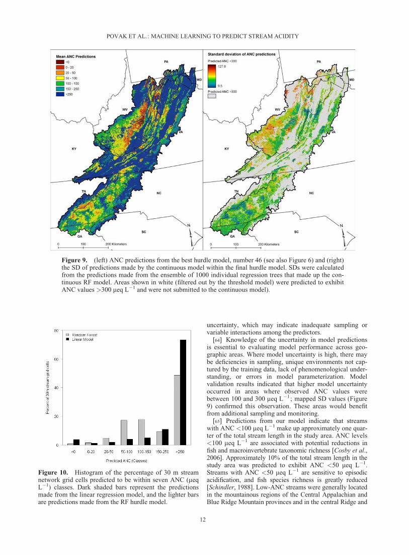
[52] Stream water chemistry often associated with bio-logical harm (e.g., ANC< 100 meq L�1) occurred through-out the study area (Figure 9). Approximately 8% of thestream network displayed ANC values <50 meq L�1, and24.5% with values <100 meq L�1 (Figure 10). Lithologicpatterns clearly influenced ANC predictions, with high-ANC areas occurring mainly in limestone valley bottoms,and low ANC occurring on siliceous bedrock.
[53] We compared predictions from RF hurdle models tothose from a linear regression model (LM). Differences in
the patterns of predictions made by the LM and RF hurdlemodel were apparent. The LM predicted >84% of thestream network (as measured by length) had ANC values>150 meq L�1, compared to only 58% for the RF hurdlemodel (Figure 10). The RF model predicted 35% of streamshad ANC between values 50 and 150 meq L�1 compared toonly 8.9% predicted by LM (Figure 10). For the mostacidic class (i.e., ANC< 0 meq L�1), the LM predicted aslightly higher percentage of streams (3.9% LM versus0.9% RF hurdle).
[54] LM tended to predict higher ANC levels particularlyin the central Appalachian region (Figures S5 and S6).However, in the southern Blue Ridge and in pockets ofeastern and central West Virginia, where the RF hurdlemodel predicted low ANC rates (e.g., ANC< 50 meq L�1),the LM generally predicted very low ANC rates (FiguresS5 and S6). Low ANC predictions from the LM were fairlyisolated geographically and generally corresponded to areasof highest sampling intensity, potentially indicating that theLM had poor predictive ability outside the limits of thetraining data.
Figure 6. Response curves showing relations between the predicted ANC and individual predictor var-iables included in the threshold model within the hurdle modeling framework. Black tick marks on the xaxis indicate decile classes for the predictors. The y axis indicates the relative effect of the predictor onANC on a logit scale. In general, higher y-axis values indicate a higher probability of predicting a lowANC value. See Table S1 for a description of predictors.
POVAK ET AL.: MACHINE LEARNING TO PREDICT STREAM ACIDITY
9
[55] Spatial patterning of RF model uncertainty was alsoapparent across the study area. Model uncertainty wasexpressed as the SD of continuous predictions made amongthe ensemble of individual trees comprising the RF model.As might be expected, model uncertainty was highest in thewestern portion of the study domain where few samplesoccurred (Figure 9) and lowest in the areas with the mostsamples.
4. Discussion
4.1. Modeling Low ANC
[56] Biogeochemical and climatic influences on ANCalmost certainly involve many interactions among environ-mental and climatic processes that together influence theultimate susceptibility of a stream to the acidifying effects ofS deposition. Some of these factors are as yet unknown, andothers are known, but complex, nonlinear, nonstationaryover space and time, and difficult to measure [Driscoll et al.,1987; United States Environmental Protection Agency,2009]. Known processes include (1) nutrient uptake by
plants, transport of litter fall, and delivery to neighboringstreams; (2) mobilization of Al3þ ; (3) erosion and sedimen-tation of cations and anions from upslope catchments; (4)deposition of S from exogenous sources; and (5) physicaland chemical weathering of parent materials proximal anddistal to the stream channel [Christophersen and Neal,1990; Driscoll et al., 1987; Johnson and Host, 2010; Reusset al., 1987; Sullivan, 2000]. Modeling the susceptibility ofaquatic systems to acidic deposition at a regional scalerequires an understanding of these processes, access toadequately resolved data layers that accurately portray thecomplexity of environmental conditions, and reliable statisti-cal modeling.
[57] Our aim was to predict how integrated biological,geological, chemical, and climatic processes within catch-ments can be used to predict stream water chemistry, whichhas linear flow properties that may concentrate or dilutelocal buffering capacity within stream networks, and whichresult in a unique correlation structure among observedresponses and the environments driving the response.Results from this study indicated that predictions of ANC
Figure 7. Response curves showing relations between the predicted ANC and individual predictor var-iables included in the continuous model within the hurdle modeling framework. Black tick marks on xaxis indicate decile classes for the predictors. The y axis indicates the relative effect of the predictors onANC. In general, lower y-axis values indicate lower ANC values. Note that the majority of climate varia-bles have been multiplied by a constant, which had no effect on predictions or model performance. SeeTable S1 for a description of the predictor variables.
POVAK ET AL.: MACHINE LEARNING TO PREDICT STREAM ACIDITY
10
within a region can be made using a combination ofremotely sensed, spatially explicit environmental data, arepresentative sample of water chemistry across the region,and a modeling framework appropriate for the analysis.
[58] We addressed several aspects of the environmentaland stream water chemistry during the modeling processincluding the spatial scale of the environmental predictors,the timespan over which water chemistry was sampled, andthe spatial distribution of water sample sites.
[59] Stream water chemistry is governed by biologicaland physical processes that are both endogenous and exog-enous to the contributing watersheds [Sullivan et al., 2007].Water chemistry may be sampled at points along streams,but the environmental and edaphic influences on that chem-istry must be related to the contributing space assignable tothose points [Johnson and Host, 2010; Steel et al., 2010].We accounted for this by using an upslope-averaging tech-nique [McDonnell et al., 2012] that generated values forpredictor variables that reflected conditions over the con-tributing area to each point along the stream network. Point
estimates of the biogeoclimatic setting at the location ofwater chemistry sample points would not adequately repre-sent catchment level influences on water chemistry.
[60] The water chemistry data used in this study wereobtained from a series of sampling efforts undertaken inter-mittently over a span of years (1986–2009). These datawere used because they were readily available, sampled afairly large spatial extent, were collected at fairly high den-sity, and used a consistent method for calculating streamwater acid-base status. All sample data used for modelingwere collected during spring flow. As such, the model rep-resents a description of the environment expected to influ-ence spring season ANC concentrations, which are oftenthe lowest that occur in these streams [Herlihy et al., 1993].Although S deposition declined substantially between 1986and 2009, stream water ANC has shown little recovery,mainly because of base cation depletion and continued Sadsorption on soils [Sullivan et al., 2011, 2008, 2004]. As aresult, we expect that data collected over a period of two dec-ades generally reflect ambient stream acid-base chemistry.
[61] The lack of an a priori sampling design necessitatedan assessment of potential sampling bias. The effects ofdata resampling on model prediction were mixed. Modelsthat undersampled low-ANC sites (the majority sample)reduced RMSE but increased threshold model error rates.Models that oversampled high-ANC sites (the minoritysample) produced negligible differences in model perform-ance (Figure 8). Hence, rebalancing the sample wasunnecessary, and RF models performed reasonably well,even with unbalanced sampling. Our results suggest thatthe multivariate signature of low ANC was unique enoughto be readily detected against the background noise of otherANC levels. Moreover, the RF and boosted models consis-tently outperformed traditional regression approaches, andtwo-stage hurdle modeling adequately minimized effects ofsampling bias on predicted ANC.
[62] Comparison of mean RMSE values for RF modelswith and without hurdle modeling showed that the hurdlemodel provided a more than twofold decrease in modelRMSE (258.1, RF-only, and 107.5, hurdle model). TheRMSE for ANC predictions <150 meq L�1 was 36.6 meqL�1. This observation is key: we can accept higher errorrates in predictions of high ANC but require more accuratepredictions where ANC values are within the range ofknown ecological degradation. Model performance wassubstantially improved for the ANC conditions that aremost biologically relevant (�100 meq L�1).
[63] A major aim of ecological models is often to predictvarious phenomena or responses over large geographicareas. When models produce sufficiently accurate predic-tions, they provide valuable insight into pattern and processinteractions, and variability of those interactions. Ourmodel allowed us to (1) identify areas of potential concernfor ecological remediation and management ; (2) identifydiscrete areas where exogenous factors such as the broad-scale climatic setting or large areas of heavy acidic S depo-sition may trump local factors such as topography or soils(e.g., the western portion of the region where ANC predic-tions were low despite deeply dissected topography; pre-sumably due to precipitation and S deposition patterns) ; (3)identify areas where spatial clustering of environmentaldegradation is predicted; and (4) locate areas of high
Figure 8. Scatterplot of the performance of 48 RF contin-uous models varying by combination of data resamplingmethod (3), ANC threshold (4), and probability threshold(4). Validation statistics are based on predictions to a ran-domly drawn 25% subset of the data. A complete list ofmodel results is included in Table S2. Model number 46,which showed the lowest RMSE and percent misclassified,was used as the final model.
Table 2. Results From a Moran’s I Correlogram on Model Resid-uals From the Hurdle Modela
aValues represented in bold indicate significant autocorrelation.
POVAK ET AL.: MACHINE LEARNING TO PREDICT STREAM ACIDITY
11
uncertainty, which may indicate inadequate sampling orvariable interactions among the predictors.
[64] Knowledge of the uncertainty in model predictionsis essential to evaluating model performance across geo-graphic areas. Where model uncertainty is high, there maybe deficiencies in sampling, unique environments not cap-tured by the training data, lack of phenomenological under-standing, or errors in model parameterization. Modelvalidation results indicated that higher model uncertaintyoccurred in areas where observed ANC values werebetween 100 and 300 meq L�1; mapped SD values (Figure9) confirmed this observation. These areas would benefitfrom additional sampling and monitoring.
[65] Predictions from our model indicate that streamswith ANC <100 meq L�1 make up approximately one quar-ter of the total stream length in the study area. ANC levels<100 meq L�1 are associated with potential reductions infish and macroinvertebrate taxonomic richness [Cosby et al.,2006]. Approximately 10% of the total stream length in thestudy area was predicted to exhibit ANC <50 meq L�1.Streams with ANC <50 meq L�1 are sensitive to episodicacidification, and fish species richness is greatly reduced[Schindler, 1988]. Low-ANC streams were generally locatedin the mountainous regions of the Central Appalachian andBlue Ridge Mountain provinces and in the central Ridge and
Figure 9. (left) ANC predictions from the best hurdle model, number 46 (see also Figure 6) and (right)the SD of predictions made by the continuous model within the final hurdle model. SDs were calculatedfrom the predictions made from the ensemble of 1000 individual regression trees that made up the con-tinuous RF model. Areas shown in white (filtered out by the threshold model) were predicted to exhibitANC values >300 meq L�1 and were not submitted to the continuous model).
Figure 10. Histogram of the percentage of 30 m streamnetwork grid cells predicted to be within seven ANC (meqL�1) classes. Dark shaded bars represent the predictionsmade from the linear regression model, and the lighter barsare predictions made from the RF hurdle model.
POVAK ET AL.: MACHINE LEARNING TO PREDICT STREAM ACIDITY
12
Valley Province (Figure 9). These areas are characterized byrugged topography, relatively steep temperature and precipi-tation gradients, high percentage of forest cover, and a vari-ety of geologic parent materials.
[66] In lieu of using a statistical modeling approach, pre-vious estimates of regional stream water ANC in our studyarea have been made using stratified random samplingdesigned to evaluate the proportion of surveyed streamscontained within specified ANC classes [Herlihy et al.,1993]. Estimates from these surveys generally corroborateour findings when individual ecoregions are assessed,although direct comparison is not possible. The authorsconcluded that about 13%–25% of the sample streams dis-played ANC values <50 meq L�1; our area prediction waslower (<10%).
4.2. Endogenous and Exogenous Drivers of StreamWater Acidity
[67] Results from the ANC modeling suggested lowANC of streams in the southern Appalachian Mountainregion derived from lithologies, land-surface forms, tem-perature and precipitation regimes, exogenous S deposition,and endogenous patterns of physiognomies, soils, and top-ographies within catchments.
[68] Streams situated on siliceous lithologies had rela-tively low ANC, and this variable was the strongest predic-tor in the continuous model. Other studies have also foundstrong empirical relationships between lithology and streamwater ANC [Herlihy et al., 1993; Puckett and Bricker,1992; Sullivan et al., 2007]. Soils created from siliceousmaterials tend to be shallow, acidic [Krug and Frink,1983], and generally exhibit low productivity, conductivity,and BCw [Herlihy et al., 1993]. Despite the known impor-tance of lithology on governing stream water quality andother ecological processes, regionwide data layers describ-ing mineralogy [NRCS Soil Survey Staff, 2010a] are ofinconsistent quality and resolution [Sullivan et al., 2007].For instance, areas of West Virginia and Georgia delineatemineralogy at different resolutions, which likely contrib-utes to reduced model performance in these areas (Figure9). Because lithology and soil characteristics were impor-tant predictors in both the threshold and continuous models(Table 1), we suspect that improved quality, resolution, andconsistency in soil and geologic data would improve modelprediction and spatial accuracy.
[69] Low ANC was also associated with a high percent-age of forest cover (Figures 6 and 7). Sullivan et al. [2007]and Herlihy et al. [1998] found a similar relationshipbetween low ANC and high forest cover for streams withinour study area. Afforested areas in Europe have also beenfound to consistently incite high levels of acidity in soilsand stream water [Gee and Stoner, 1989; Jenkins et al.,1990; Miles, 1986; Whitehead et al., 1988]. Forests canhave a variable influence on water chemistry depending onthe prevailing climate, underlying geology, catchment size,successional stage of forest development, forest composi-tion, and legacy influences of past disturbances, amongothers [Harriman and Morrison, 1982; Sullivan, 2000].Forests generally scavenge wet and dry deposition ofatmospheric pollutants (including, but not limited to S)and translate these pollutants to watershed soils and theassociated stream reach. Furthermore, forests can take up
base cations and reduce the capacity of soils to bufferagainst acidic inputs. However, forested areas in the Appa-lachian region are generally located at higher elevationsand on ridges where catchments are small and reside on si-liceous bedrocks [Herlihy et al., 1993]. Therefore, the geo-graphic locations of forested areas may be coincident withareas predisposed to having low ANC due to the edaphicand lithologic setting.
[70] When high-elevation sites were modeled alone, per-cent coniferous forest cover was the leading variable in themodel, followed by deciduous forest cover. Moreover,these cover types displayed opposite influences on ANC(i.e., high coniferous cover was associated with low ANC,and high deciduous cover was related to high ANC; FigureS4). This observation is generally consistent with otherworks [Cronan et al., 1978; Nihlgård, 1970]. Indeed, high-elevation catchments dominated by deciduous forest(�60% cover; threshold value, Figure S4) had mean ANCof 83.8 meq L�1, compared to �19.8 meq L�1 for catch-ments with a lesser deciduous component. In our data sethigh-elevation deciduous forests were generally located inlarger catchments, with a lower percentage of siliceous par-ent material, less dry S deposition, and warmer and drierclimates than coniferous forests. Whether coniferous foresttypes contributed to low ANC at higher elevations throughacidic foliage deposition, pollutant sequestration, and sub-sequent acidic throughfall and stemflow [Dunford et al.,2012; Miles, 1986], or if the environmental setting of co-niferous forests influenced low ANC remains unclear. It isplausible that the influences of catchment size, mineral sub-strate, weathering rates, and dominant vegetation are highlyinteractive and change across the study region. The contin-uous model in our study identified important interactionsamong forest cover and lithology, and ANC was higher incatchments dominated by siliceous lithology when forestcover was low, compared to well-forested catchments withsimilar lithologies (Figure S2).
[71] Although elevation is generally considered a surro-gate for climate at broad scales, elevation was not explicitlyincluded as a predictor variable because remotely sensedclimate data are now regionally available at a scale and ac-curacy sufficient for our application. Predictive modeling ismost robust when predictor variables expected to bedirectly linked to the modeled response are used in place ofthose that may have indirect effects [Austin, 2002]. Forexample, elevation is often included as a predictor in spe-cies distribution modeling [Austin, 2002], but rarely do spe-cies respond to elevation alone. Rather, more directpredictors such as temperature and precipitation, which of-ten are correlated with elevation, are more directly relatedto a species’ distributional limits [Austin, 2002; Elith andLeathwick, 2009].
[72] Elevation is often used as a predictor in the ANC lit-erature, where increases in elevation are often associatedwith (1) increased S deposition [Lawrence et al., 1999], (2)higher precipitation [Sullivan et al., 1999], (3) cooler tem-peratures, (4) higher percent siliceous parent material, (5)thinner and coarser soils with lower cation exchangecapacity, (6) smaller catchments with steep slopes, and (7)higher percent forest cover [Herlihy et al., 1998, 1993;Lynch and Dise, 1985; Sullivan et al., 2007], all of whichlead to decreased surface water ANC [Herlihy et al., 1993;
POVAK ET AL.: MACHINE LEARNING TO PREDICT STREAM ACIDITY
13
Sullivan et al., 2007; Sullivan et al., 2011]. However, it isnot clear how these factors rank in importance in drivingANC at regional scales.
[73] Our modeling results indicated that elevation waseither uncorrelated or loosely correlated with stream waterANC (r¼�0.21), total S deposition (r¼ 0.11), percent sili-ceous lithology (r¼�0.04), soil depth (r¼ 0.06), soil clay(r¼�0.26), catchment size (r¼�0.09), and forest cover(r¼�0.01). However, elevation was correlated with some,but not all, climate variables. These variables included num-ber of days >32�C (AB90GROW, r¼�0.70), nongrowingseason precipitation levels (r¼ 0.63), number of days with-out precipitation (NPDAYMAX, r¼�0.63), number ofhumid days (VWDAYMAX, r¼ 0.70), nongrowing seasonsolar insolation (SOLARTOTNG, r¼ 0.61), and nongrow-ing season gross primary productivity (GPPNG, r¼ 0.60).Three of these climate variables (NPDAYMAX, VWDAY-MAX, and AB90GROW) were among the top five variablesin the continuous model in our study and indicated that low-ANC streams coincided with areas that experience fewprecipitation-free days, few dry days, and few days >32�C.These variables had higher variable importance scores thanother edaphic, topographic, vegetation, and sulfur depositionvariables in the model, suggesting that climate may drive re-gional stream water acidity.
[74] The importance of identifying climatic correlates ofstream water ANC with our models has implications formonitoring and continued modeling of future stream wateracid-base chemistry [Ben�cokov�a et al., 2011; Evans, 2005;Wright et al., 2006]. Climate projections for the southernAppalachian Mountain region indicate both warmer anddrier (south) and warmer and wetter (north) futures (year2100 projections) [Hayhoe et al., 2008; Karl et al., 2009;Solomon, 2007]. ANC modeling results reported here indi-cate that areas with relatively low precipitation and warmtemperatures have relatively high stream water ANC. Awarmer climate would increase BCw and therefore streamANC. Drier conditions would decrease wet S depositionand leaching losses of base cations from soils. Interactionsfrom the continuous model (Figure S2) suggest that highertemperatures and lower precipitation can moderate theinfluence of siliceous lithology on reducing stream waterANC levels. Monitoring ANC over time will be necessaryto better understand these interactions.
[75] Ecosystem responses to longer-term climatic changeare largely unknown due to the potential complexity ofinteractions among the changes. Accompanying changes intemperature, precipitation, and insolation regimes, changesin overall productivity, vegetative communities, plantcover, carbon and nutrient uptake by plants, and influencesof disturbances may all affect the acid-base chemistry ofstreams within the study domain. Thus, it will be importantto continue to monitor and model ANC. Moreover, newcombinations or changes in the importance of predictorswill likely necessitate water chemistry sampling that moreevenly samples the variability of conditions represented bythe predictors.
[76] Since enactment of the Clean Air Act Amendmentsof 1990, levels of S deposition in the eastern United Stateshave decreased by more than 40% [Baumgardner et al.,2002]. Ongoing monitoring suggests that reduced depositionimproved stream and lake acid-base chemistry at some loca-
tions [United States Environmental Protection Agency,2009]. In the current assessment, the amount of S depositedwas an important predictor of ANC, but S deposition wasonly included in one model (the continuous model) and wasnot included in any other of the models in the analysis.Instead, other variables related to the surrounding geology,soils, climate, and vegetation were generally more influentialthan the amount of S deposition in the catchment.
[77] Furthermore, the continuous model did not indicatea monotonic decrease in ANC with increasing levels of Sdeposition; rather, nonlinearities in this relation were appa-rent. Modeled ANC was lowest for intermediate levels ofdry S deposition, pointing to interactions among S andother predictors. For example, intermediate levels of dry Sdeposition typically occurred in montane environments,where wet deposition was highest, catchment areas weresmall, and climate was cool and moist with frequent cloudcover. These interactions were nonstationary across thestudy domain and could not be accounted for using a singleglobal model.
[78] Nonlinearities may also derive from the rathercoarse resolution of CMAQ modeled dry and wet S deposi-tion or from CMAQ prediction errors. Considerable uncer-tainty exists in these layers, but it is difficult to quantify theextent of these uncertainties as no ‘‘true estimates’’ of dep-osition exist to test model errors [United States Environ-mental Protection Agency, 2009].
[79] Another possible explanation for the predicted non-linear relationship between S deposition and ANC may berelated to the temporal discontinuity between a portion ofthe observed ANC data and the modeled CMAQ data.Because the water chemistry data were taken over a 24year period and the CMAQ data used to represent dry Sdeposition were taken from 2002, the modeled dry S depo-sition may not accurately represent conditions at the timeof the water chemistry sampling. However, CMAQ data for2002 likely represent the relative extent to which eachcatchment has been exposed to elevated S deposition. Fur-thermore, base cation depletion of soils has limited theANC recovery of the most acid-sensitive streams [Sullivanet al., 2004, 2011]. Nevertheless, results here indicate thatreductions in S inputs alone may not lead directly toincreases in stream water ANC because interactions withother driving variables, such as temperature and precipita-tion, confound simple monotonic interpretation of relationsbetween acidic S inputs and stream water ANC.
5. Conclusion
[80] Models developed here predict stream water ANCacross the southern Appalachian Mountains. Results suggestthat aquatic biota may be at risk from the deleterious effectsof low ANC (ANC< 100 meq L�1) [Sullivan, 2000] overapproximately one fourth of the stream network. Acid-sensitive areas have siliceous lithology, cool and moist cli-mates, and forests with low soil clay and pH levels, and rela-tively small contributing areas. Our findings suggest thatpredicting future ANC will require incorporation of datafrom ongoing stream water chemistry monitoring into amodeling framework capable of quantifying the inherentlynonlinear interactions among relevant biogeochemical andclimatic variables. Continued water chemistry monitoring
POVAK ET AL.: MACHINE LEARNING TO PREDICT STREAM ACIDITY
14
should include previously sampled locations and beexpanded to include undersampled geographic areas andenvironments (e.g., areas with high model uncertainty).Although correlation does not imply causation, the identifi-cation of several climate variables as key drivers of ANCsuggests that future climate change may influence futurestream acid-base chemistry in unique and complex ways.The analysis approach taken here can be readily applied inother regions where adequate coverage of high-resolution,spatially explicit environmental data is available, and wherestream water quality surveys have been conducted at a rea-sonable sampling intensity.
ReferencesAustin, M. (2002), Spatial prediction of species distribution: An interface
between ecological theory and statistical modelling, Ecol. Model.,157(2–3), 101–118.
Barandela, R., E. Rangel, J. S�anchez, and F. Ferri (2003), Restricted decon-tamination for the imbalanced training sample problem, in Progress inPattern Recognition Research, edited by A. Sanfeliu and J. Ruiz-Shulcl-oper, pp. 424–431, Springer, Berlin.
Baumgardner, R. E., T. F. Lavery, C. M. Rogers, and S. S. Isil (2002), Esti-mates of the atmospheric deposition of sulfur and nitrogen species:Clean air status and trends network, 1990–2000, Environ. Sci. Technol.,36(12), 2614–2629.
Ben�cokov�a, A., J. Hru�ska, and P. Kr�am (2011), Modeling anticipated cli-mate change impact on biogeochemical cycles of an acidified headwatercatchment, Appl. Geochem., 26, suppl., S6–S8.
Bivand, R., L. Anselin, O. Berke, A. Bernat, M. Carvalho, Y. Chun, C.Dormann, S. Dray, R. Halbersma, and N. Lewin-Koh (2011), spdep:Spatial dependence: Weighting schemes, statistics and models, RPackage Version 0.5–31. [Available at http://cran.r-project.org/web/packages/spdep/index.html.].
Breiman, L. (1984), Classification and Regression Trees, Chapman & Hall/CRC, New York, N. Y.
Breiman, L. (2001a), Random forests, Mach. Learn., 45(1), 5–32.Breiman, L. (2001b), Statistical modeling: The two cultures (with com-
ments and a rejoinder by the author), Stat. Sci., 16(3), 199–231.Byun, D., and K. L. Schere (2006), Review of the governing equations,
computational algorithms, and other components of the models: 3. Com-munity Multiscale Air Quality (CMAQ) modeling system, Appl. Mech.Rev., 59(2), 51–77.
Chawla, N. V., K. W. Bowyer, L. O. Hall, and W. P. Kegelmeyer (2002),SMOTE: Synthetic minority over-sampling technique, J. Artif. Intell.Res., 16(1), 321–357.
Christophersen, N., and C. Neal (1990), Linking hydrological, geochemical,and soil chemical processes on the catchment scale: An interplay betweenmodeling and field work, Water Resour. Res., 26(12), 3077–3086.
Christophersen, N., C. Neal, and J. Mulder (1990), Reversal of stream acidi-fication at the Birkenes catchment, southern Norway: Predictions basedon potential ANC changes, J. Hydrol., 116(1–4), 77–84.
Clark, J. M., A. Heinemeyer, P. Martin, and S. H. Bottrell (2012), Processescontrolling DOC in pore water during simulated drought cycles in six dif-ferent UK peats, Biogeochemistry, 109(1–3), 253–270.
Cosby, B., G. Hornberger, J. Galloway, and R. Wright (1985), Modeling theeffects of acid deposition: Assessment of a lumped parameter model ofsoil water and streamwater chemistry, Water Resour. Res., 21(1), 51–63.
Cosby, B., J. Webb, J. Galloway, and F. Deviney (2006), Acidic depositionimpacts on natural resources in Shenandoah National Park, Tech. Rep.NPS/NER/NRTR-2006/066, Philadelphia, Pa.
Cronan, C. S., W. A. Reiners, R. C. Reynolds, and G. E. Lang (1978), For-est floor leaching: Contributions from mineral, organic, and carbonicacids in New Hampshire subalpine forests, Science, 200(4339), 309–311.
De’ath, G. (2007), Boosted trees for ecological modeling and prediction,Ecology, 88(1), 243–251.
De’ath, G., and K. E. Fabricius (2000), Classification and regression trees:A powerful yet simple technique for ecological data analysis, Ecology,81(11), 3178–3192.
Driscoll, C. T., B. J. Wyskowski, C. C. Cosentini, and M. E. Smith (1987),Processes regulating temporal and longitudinal variations in the chemis-
try of a low-order woodland stream in the Adirondack Region of NewYork, Biogeochemistry, 3(1/3), 225–241.
Driscoll, C. T., K. M. Driscoll, K. M. Roy, and M. J. Mitchell (2003),Chemical response of lakes in the Adirondack region of New York todeclines in acidic deposition, Environ. Sci. Technol., 37(10), 2036–2042.
Duan, L., J. Hao, S. Xie, and K. Du (2000), Critical loads of acidity for sur-face waters in China, Sci. Total Environ., 246(1), 1–10.
Dunford, R. W., D. N. M. Donoghue, and T. P. Burt (2012), Forest landcover continues to exacerbate freshwater acidification despite decline insulphate emissions, Environ. Pollut., 167, 58–69.
Elith, J., and J. R. Leathwick (2009), Species distribution models: Ecologi-cal explanation and prediction across space and time, Ann. Rev. Ecol.Evol. Syst., 40, 677–697.
Elith, J., J. Leathwick, and T. Hastie (2008), A working guide to boostedregression trees, J. Anim. Ecol., 77(4), 802–813.
Evans, C. D. (2005), Modelling the effects of climate change on an acidicupland stream, Biogeochemistry, 74(1), 21–46.
Franklin, J., and J. A. Miller (2009), Mapping Species Distributions: Spa-tial Inference and Prediction, Cambridge Univ. Press, New York, NY.
Gahegan, M. (2003), Is inductive machine learning just another wild goose(or might it lay the golden egg)?, Int. J. Geogr. Inf. Sci., 17(1), 69–92.
Galloway, J. (2001), Acidification of the world: Natural and anthropogenic,Water Air Soil Pollut., 130(1), 17–24.
Galloway, J. N., Z. Dianwu, X. Jiling, and G. E. Likens (1987), Acid rain:China, United States, and a remote area, Science, 236(4808), 1559–1562.
Gee, A., and J. Stoner (1989), A review of the causes and effects of acidifi-cation of surface waters in Wales and potential mitigation techniques,Arch. Environ. Contam. Toxicol., 18(1), 121–130.
Grimm, J. W., and J. A. Lynch (2004), Enhanced wet deposition estimatesusing modeled precipitation inputs, Environ. Monit. Assess., 90(1), 243–268.
Guerold, F., J.-P. Boudot, G. Jacquemin, D. Vein, D. Merlet, and J. Rouiller(2000), Macroinvertebrate community loss as a result of headwaterstream acidification in the Vosges Mountains (N-E France), Biodivers.Conserv., 9(6), 767–783.
Hargrove, W., and F. Hoffman (2004), A flux atlas for representativenessand statistical extrapolation of the Ameriflux network, Oak Ridge Natl.Lab. Tech. Memo. ORNL-TM-2004/112, pp. 1–152.
Harriman, R., and B. Morrison (1982), Ecology of streams draining forestedand non-forested catchments in an area of central Scotland subject toacid precipitation, Hydrobiologia, 88(3), 251–263.
Hastie, T., R. Tibshirani, J. Friedman, and J. Franklin (2005), The elementsof statistical learning: Data mining, inference and prediction, Math.Intell., 27(2), 83–85.
Hayhoe, K., C. Wake, B. Anderson, X. Z. Liang, E. Maurer, J. Zhu, J. Brad-bury, A. DeGaetano, A. M. Stoner, and D. Wuebbles (2008), Regionalclimate change projections for the Northeast USA, Mitig. Adapt. Strat.Global Change, 13(5), 425–436.
He, H., and E. A. Garcia (2009), Learning from imbalanced data, IEEETrans. Knowl. Data Eng., 21(9), 1263–1284.
Hendershot, W. H., P. Warfvinge, F. Courchesne, and H. U. Sverdrup(1991), The mobile anion concept—Time for a reappraisal?, J. Environ.Qual., 20(3), 505–509.
Henriksen, A., and M. Posch (2001), Steady-state models for calculatingcritical loads of acidity for surface waters, Water Air Soil Pollut.: Focus,1(1), 375–398.
Henriksen, A., M. Posch, H. Hultberg, and L. Lien (1995), Critical loads ofacidity for surface waters: Can the ANC limit be considered variable?,Water Air Soil Pollut., 85(4), 2419–2424.
Herlihy, A. T., P. R. Kaufmann, M. R. Church, P. J. Wigington Jr., J. R.Webb, and M. J. Sale (1993), The effects of acidic deposition on streamsin the Appalachian Mountain and Piedmont Region of the Mid-AtlanticUnited States, Water Resour. Res., 29(8), 2687–2703.
Herlihy, A. T., J. L. Stoddard, and C. B. Johnson (1998), The relationshipbetween stream chemistry and watershed land cover data in the mid-Atlantic region, US, Water Air Soil Pollut., 105(1), 377–386.
Homer, C., J. Dewitz, J. Fry, M. Coan, N. Hossain, C. Larson, N. Herold, A.McKerrow, J. N. VanDriel, and J. Wickham (2007), Completion of the2001 National Land Cover Database for the conterminous United States,Photogramm. Eng. Remote Sens., 73(4), 337–341.
Hru�ska, J., F. Moldan, and P. Kr�am (2002), Recovery from acidification incentral Europe—Observed and predicted changes of soil and stream-water chemistry in the Lysina catchment, Czech Republic, Environ. Pol-lut., 120(2), 261–274.
POVAK ET AL.: MACHINE LEARNING TO PREDICT STREAM ACIDITY
Jenkins, A., B. J. Cosby, R. C. Ferrier, T. A. B. Walker, and J. D. Miller(1990), Modelling stream acidification in afforested catchments: Anassessment of the relative effects of acid deposition and afforestation,J. Hydrol., 120(1–4), 163–181.
Jenness, J. S. (2004), Calculating landscape surface area from digital eleva-tion models, Wildlife Soc. B., 32(3), 829–839.
Jenson, S., and J. Domingue (1988), Extracting topographic structure fromdigital elevation data for geographic information system analysis, Photo-gramm. Eng. Remote Sens., 54(11), 1593–1600.
Johnson, L. B., and G. E. Host (2010), Recent developments in landscapeapproaches for the study of aquatic ecosystems, J. North Am. Benthol.Soc., 29(1), 41–66.
Karl, T. R., J. M. Melillo, and T. C. Peterson (2009), Global Climate ChangeImpacts in the United States, Cambridge Univ. Press, New York, NY.
Krug, E. C., and C. R. Frink (1983), Acid rain on acid Soil : A new perspec-tive, Science, 221(4610), 520–525.
Lawrence, G. B., M. B. David, G. M. Lovett, P. S. Murdoch, D. A. Burns,J. L. Stoddard, B. P. Baldigo, J. H. Porter, and A. W. Thompson (1999),Soil calcium status and the response of stream chemistry to changingacidic deposition rates, Ecol. Appl., 9(3), 1059–1072.
Levin, S. (1992), The problem of pattern and scale in ecology: The RobertH. MacArthur award lecture, Ecology, 73(6), 1943–1967.
Liaw, A., and M. Wiener (2002), Classification and regression by random-Forest, R News, 2(3), 18–22.
Lien, L., G. Raddum, and A. Fjellheim (1992), Critical loads of acidity tofreshwater fish and invertebrates, Naturens Talegrenser 23.
Lynch, D. D., and N. B. Dise (1985), Sensitivity of stream basins in Shenan-doah National Park to acid deposition, Rep. 85–4115, U.S Dep. of theInter., U.S. Geol. Surv., Richmond, Va.
Maclure, M., and W. C. Willet (1987), Misinterpretation and misuse of theKappa statistic, Am. J. Epidemiol., 126(2), 161–169.
McDonnell, T., B. Cosby, T. Sullivan, S. McNulty, and E. Cohen (2010), Com-parison among model estimates of critical loads of acidic deposition usingdifferent sources and scales of input data, Environ. Pollut., 158, 2934–2939.
McDonnell, T. C., B. J. Cosby, and T. J. Sullivan (2012), Regionalizationof soil base cation weathering for evaluating stream water acidificationin the Appalachian Mountains, USA, Environ. Pollut., 162, 338–344.
Menz, F. C., and H. M. Seip (2004), Acid rain in Europe and the UnitedStates: An update, Environ. Sci. Policy, 7(4), 253–265.
Miles, J. (1986), What are the effects of trees on soils?, in Trees and Wild-life in the Scottish Uplands, edited by D. Jenkins, pp. 55–62, NERC/ITE,Swindon, UK.
Moore, I. D., P. E. Gessler, G. A. Nielsen, and G. A. Peterson (1993), Soil attrib-ute prediction using terrain analysis, Soil Sci. Soc. Am. J., 57(2), 443–452.
National Atlas of the United States (2006), Federal Lands of the UnitedStates: National Atlas of the United States, Reston, Va.
Neal, C., B. Reynolds, and A. J. Robson (1999), Acid neutralisationcapacity measurements within natural waters: Towards a standardisedapproach, Sci. Total Environ., 243–244, 233–241.
Nihlgård, B. (1970), Precipitation, its chemical composition and effect onsoil water in a beech and a spruce forest in south Sweden, Oikos, 21,208–217.
Nilsson, J., and P. Grennfelt (1988), Critical Loads for Sulfur and Nitrogen,31 pp., Nordic Counc. of Minist., Copenhagen, Denmark.
NRCS Soil Survey Staff (2010a), Soil Survey Geographic (SSURGO) data-base for southern Appalachian Region. Available online at http://soilda-tamart.nrcs.usda.gov. Accessed [October/10/2010].
NRCS Soil Survey Staff (2010b), U.S. General Soil Map State Soil Geo-graphic (STATSGO) database for the southern Appalachian Region.Available online at http://soildatamart.nrcs.usda.gov. Accessed [Octo-ber/10/2010].
Olden, J. D., J. J. Lawler, and N. Poff (2008), Machine learning methodswithout tears: A primer for ecologists, Q. Rev. Biol., 83(2), 171–194.
Omernik, J. M. (1987), Ecoregions of the conterminous United States, Ann.Assoc. Am. Geogr., 77(1), 118–125.
Prasad, A. M., L. R. Iverson, and A. Liaw (2006), Newer classification andregression tree techniques: Bagging and random forests for ecologicalprediction, Ecosystems, 9(2), 181–199.
Puckett, L. J., and O. P. Bricker (1992), Factors controlling the major ionchemistry of streams in the blue ridge and valley and ridge physiographicprovinces of Virginia and Maryland, Hydrol. Processes, 6(1), 79–97.
R Development Core Team (2011), R: A Language and Environment forStatistical Computing, Vienna, Austria.
Rago, P. J., and J. G. Wiener (1986), Does pH affect fish species richnesswhen lake area is considered?, Trans. Am. Fish. Soc., 115(3), 438–447.
Reuss, J. O., B. J. Cosby, and R. F. Wright (1987), Chemical processes gov-erning soil and water acidification, Nature, 329(6134), 27–32.
Reynolds, K. M., P. F. Hessburg, T. J. Sullivan, N. A. Povak, T. C. McDon-nell, B. J. Cosby, and W. Jackson (2012), Spatial decision support forassessing impacts of atmospheric sulfur deposition on aquatic ecosys-tems in the southern Appalachian Region, paper presented at 45th annualHawaii International Conference on System Sciences, IEEE, Wailea,Maui, Hawaii, 4–7 January.
Ridgeway, G. (2006), Generalized boosted regression models, Documenta-tion on the R Package ‘gbm’, Version 1�5, 7.
Schindler, D. W. (1988), Effects of acid rain on freshwater ecosystems,Science, 239(4836), 149–157.
Schöpp, W., M. Posch, S. Mylona, and M. Johansson (2003), Long-termdevelopment of acid deposition (1880–2030) in sensitive freshwaterregions in Europe, Hydrol. Earth Syst. Sci., 7(4), 436–446.
Solomon, S. (2007), Climate Change 2007: The Physical Science Basis: Contri-bution of Working Group I to the Fourth Assessment Report of the Intergov-ernmental Panel on Climate Change, Cambridge Univ. Press, New York, NY.
Steel, E. A., R. M. Hughes, A. H. Fullerton, S. Schmutz, J. A. Young,M. Fukushima, S. Muhar, M. Poppe, B. E. Feist, and C. Trautwein(2010), Are we meeting the challenges of landscape-scale riverineresearch? A review, Living Rev. Landscape Res., 4(1), 1–60.
Sullivan, T., J. Webb, K. Snyder, A. Herlihy, and B. Cosby (2007), Spatialdistribution of acid-sensitive and acid-impacted streams in relation towatershed features in the southern Appalachian Mountains, Water AirSoil Pollut., 182(1), 57–71.
Sullivan, T. J. (2000), Aquatic Effects of Acidic Deposition, CRC Press,Boca Raton, Fla.
Sullivan, T. J., D. F. Charles, J. A. Bernert, B. McMartin, K. B. Vach�e, andJ. Zehr (1999), Relationship between landscape characteristics, history,and lakewater acidification in the Adirondack Mountains, New York,Water Air Soil Pollut., 112(3), 407–427.
Sullivan, T. J., B. J. Cosby, A. T. Herlihy, J. R. Webb, A. J. Bulger, K. U.Snyder, P. F. Brewer, E. H. Gilbert, and D. L. Moore (2004), Regionalmodel projections of future effects of sulfur and nitrogen deposition onstreams in the southern Appalachian Mountains, Water Resour. Res., 40,W02101, doi:10.1029/2003WR001998.
Sullivan, T. J., B. J. Cosby, A. T. Herlihy, C. T. Driscoll, I. J. Fernandez,T. C. McDonnell, C. W. Boylen, S. A. Nierzwicki-Bauer, and K. U.Snyder (2007), Assessment of the Extent to Which Intensively StudiedLakes Are Representative of the Adirondack Mountain Region, N. Y.State Energy Res. and Dev. Auth.
Sullivan, T. J., B. J. Cosby, J. R. Webb, R. L. Dennis, A. J. Bulger, and F.A. Deviney (2008), Streamwater acid-base chemistry and critical loadsof atmospheric sulfur deposition in Shenandoah National Park, Virginia,Environ. Monit. Assess., 137(1), 85–99.
Sullivan, T. J., B. J. Cosby, W. A. Jackson, K. U. Snyder, and A. T. Herlihy(2011), Acidification and prognosis for future recovery of acid-sensitivestreams in the southern Blue Ridge Province, Water Air Soil Pollut.,219(1), 11–26.
Turner, M. (1989), Landscape ecology: The effect of pattern on process,Annu. Rev. Ecol. Syst., 20, 171–197.
United States Environmental Protection Agency (2009), Risk and ExposureAssessment for Review of the Secondary National Ambient Air Quality Stand-ards for Oxides of Nitrogen and Oxides of Sulfur: Final, U.S. EPA, Cent. forEnviron. Assess., Off. of Res. and Dev., Research Triangle Park, N. C.
United States Environmental Protection Agency and United States Geologi-cal Survey (2005), National Hydrography Dataset Plus—NHDPlus Ver-sion 1.0. Available from http://www.horizon-systems.com/NHDPlus/NHDPlusV1_home.php. Accessed on September 9, 2010.
United States Geological Survey (2005a), Preliminary integrated geologicmap databases for the United States: Kentucky, Ohio, Tennessee, andWest Virginia, Open-File Rep. 2005/1324.
United States Geological Survey (2005b), Preliminary integrated geologicmap databases for the United States: Delaware, Maryland, New York,Pennsylvania, and Virginia, Open-File Rep. 2005/1325.
Whitehead, P. G., B. Reynolds, M. Hornung, C. Neal, J. Cosby, and P. Pari-cos (1988), Modelling long term stream acidification trends in uplandWales at Plynlimon, Hydrol. Processes, 2(4), 357–368.
Wood, E. F., M. Sivapalan, and K. Beven (1990), Similarity and scale incatchment storm response, Rev. Geophys., 28(1), 1–18.
Wright, R. F., et al. (2006), Modelling the effect of climate change onrecovery of acidified freshwaters: Relative sensitivity of individualprocesses in the MAGIC model, Sci. Total Environ., 365(1–3), 154–166.
POVAK ET AL.: MACHINE LEARNING TO PREDICT STREAM ACIDITY