Machine Learning and Portfolio Optimization this paper, we consider regularizing the data-driven...

Machine Learningand

Portfolio Optimization

Gah-Yi Ban*Management Science & Operations, London Business School, Regent’s Park, London, NW1 4SA, United Kingdom.

[email protected]

Noureddine El KarouiDepartment of Statistics, University of California, Berkeley, CA 94720. [email protected]

Andrew E.B. LimDepartment of Decision Sciences & Department of Finance, National University of Singapore Business School, Singapore,

119245. [email protected]

The portfolio optimization model has limited impact in practice due to estimation issues when applied with

real data. To address this, we adapt two machine learning methods, regularization and cross-validation, for

portfolio optimization. First, we introduce performance-based regularization (PBR), where the idea is to

constrain the sample variances of the estimated portfolio risk and return, which steers the solution towards

one associated with less estimation error in the performance. We consider PBR for both mean-variance and

mean-CVaR problems. For the mean-variance problem, PBR introduces a quartic polynomial constraint,

for which we make two convex approximations: one based on rank-1 approximation and another based on

a convex quadratic approximation. The rank-1 approximation PBR adds a bias to the optimal allocation,

and the convex quadratic approximation PBR shrinks the sample covariance matrix. For the mean-CVaR

problem, the PBR model is a combinatorial optimization problem, but we prove its convex relaxation, a

QCQP, is essentially tight. We show that the PBR models can be cast as robust optimization problems with

novel uncertainty sets and establish asymptotic optimality of both Sample Average Approximation (SAA)

and PBR solutions and the corresponding e�cient frontiers. To calibrate the right hand sides of the PBR

constraints, we develop new, performance-based k-fold cross-validation algorithms. Using these algorithms,

we carry out an extensive empirical investigation of PBR against SAA, as well as L1 and L2 regularizations

and the equally-weighted portfolio. We find that PBR dominates all other benchmarks for two out of three

of Fama-French data sets.

Key words : machine learning, portfolio optimization, regularization, risk measures, robust optimization

History : First submitted: June 24, 2013. This version: August 31, 2016.

1. Introduction

Regularization is a technique that is commonly used to control the stability of a wide range of

problems. Its origins trace back to the 1960s, when it was introduced to deal with ill-posed linear

* formerly: Gah-Yi Vahn

1

Published online in Management Science Articles in Advance, 21 Nov 2016.http://dx.doi.org/10.1287/mnsc.2016.2644

Ban, El Karoui & Lim: Machine Learning & Portfolio Optimization2

operator problems. A linear operator problem is one of finding x 2X that satisfies Ax= b, where

A is a linear operator from a normed space X to a normed space Y , and b2 Y is a predetermined

constant. The linear operator problem is ill-posed if small deviations in b, perhaps due to noise,

result in large deviations in the corresponding solution. Specifically, if b changes to b�

, ||b�

� b||<�, then finding x that minimizes the functional R(x) = ||Ax � b

�

||2 does not guarantee a good

approximation to the desired solution even if � tends to zero. Tikhonov (1963), Ivanov (1962)

and Phillips (1962) discovered that if instead of minimizing R(x), the most obvious choice, one

minimizes the regularized functional

R⇤(x) = ||Ax� b�

||22 + �(�)P (x),

where P (x) is some functional and �(�) is an appropriately chosen constant, then one obtains

a sequence of solutions that does converge to the desired one as � tends to zero. Regularization

theory thus shows that whereas the self-evident method of minimizing R(x) does not work, the

non-self-evident method of minimizing R⇤(x) does.

Regularization has particularly been made known in recent years through its adoption in clas-

sification, regression and density estimation problems. The reader may be most familiar with its

recent popularity in the high-dimensional regression literature [see, for example, Candes and Tao

(2007) and Belloni and Chernozhukov (2013)]:

min�2Rp

||y�X�||2 +�P (�), (1)

where P (�) = ||�||1, y= [y1, . . . , yn]2Rn is the data on the observable, X= [X1, . . . ,Xn

]2Rn⇥p is

the vector of covariates, � 2Rp is the regression coe�cient that best fits the linear model y=X�,

and �> 0 is a parameter that controls the sparsity of the solution. The regression model (1) with

P (�) = ||�||1 is known as the Lasso model, used in high-dimensional applications where sparsity

of the solution � is desirable for interpretability and recovery purposes when p is large. Another

common model is the Tikhonov regularization function P (�) = ||�||2, which deals with issues that

arise when the data matrix X is ill-conditioned or singular.

In this paper, we consider regularizing the data-driven portfolio optimization problem, not for

sparsity or numerical stability as in Lasso or ridge regression, but for the purpose of improving the

out-of-sample performance of the solution. The portfolio optimization model we consider is:

w0 = argminw2Rp

Risk(w>X)

s.t. w>1p

= 1(w>µ=R),

(PO)

where w 2Rp is the investor’s holding on p di↵erent assets, X 2Rp denotes the relative return on

the p assets, µ = EX is the mean return vector and Risk : R! R is some measure of risk. The


investor’s wealth is normalized to 1, so w>1p

= 1, where 1p

denotes p⇥1 vector of ones, and w>µ=R

is the target return constraint, which we may or may not consider1, hence denoted in parentheses.

Note that shortselling, i.e., having w < 0, is allowed in this model. Setting Risk(w>X) = w>⌃w

we recover the classical model of Markowitz (1952) and setting Risk(w>X) = CV aR(�w>X;�),

where � 2 (0.5,1) and

CV aR(�w>X;�) :=min↵

↵+1

1��E(�w>X �↵)+, (2)

we recover the Conditional Value-at-Risk2 (CVaR) formulation of Rockafellar and Uryasev (2000).

In practice, one does not know the true distribution of X, but has access to past data: X =

[X1, . . . ,Xn

]. Assuming that these are iid, the standard data-driven approach to solving (PO) is to

solve:w

n

= argminw2Rp

[Riskn

(w>X)

s.t. w>1p

= 1(w>µ

n

=R),

(SAA)

where [Riskn

(w>X) is the sample average estimate of the Risk function and µn

= n�1P

n

i=1Xi

is the sample average return vector. This approach is befittingly known as the Sample Average

Approximation (SAA) method in the stochastic programming literature [see Shapiro et al. (2009)

for a general overview].

As is the case with ill-posed linear operator problems (which includes regression problems), the

solution to the SAA approach can be highly unstable. For the portfolio optimization problem,

the fact that the SAA allocation is highly unreliable is well-documented [see Frankfurter et al.

(1971), Frost and Savarino (1986, 1988b), Michaud (1989), Best and Grauer (1991), Chopra and

Ziemba (1993), Broadie (1993) for the Markowitz problem and Lim et al. (2011) for the mean-

CVaR problem], and has limited the wide-spread adoption of the model in practice, despite the

conferral of a Nobel Prize to Markowitz in 1990 for his seminal work.

In this paper, we propose performance-based regularization (PBR) to improve upon the per-

formance of the SAA approach to the data-driven portfolio allocation problem (SAA). The idea

is to constrain the sample variances of estimated quantities in a problem; for portfolio optimiza-

tion they are the estimated portfolio risk [Riskn

(w>X) and the estimated portfolio mean w>µn

.

The goal of PBR is to steer the solution towards one that is associated with less estimation error

in the performance. The overall e↵ect is to reduce the chance that a solution is chosen by mis-

leadingly high in-sample performance. Performance-based regularization is thus philosophically

1There is empirical evidence that ignoring the mean return constraint yields better solutions [see Jorion (1985)].

2also known as expected shortfall [Acerbi and Tasche (2002)]


di↵erent from Tikhonov regularization (whose purpose is stability of the solution) and Lasso reg-

ularization (whose purpose is sparsity) but is natural to the portfolio optimization problem where

the ultimate goal is the out-of-sample performance of the decision made.

We make four major contributions in this paper. Firstly, we propose and analyze new portfolio

optimization models by introducing performance-based regularization to the mean-variance and

mean-CVaR problems. This is an important conceptual development that extends the current

literature on portfolio optimization. For the mean-variance problem, the PBR model involves a

quartic polynomial constraint. Determining whether such a model is convex or not is an NP-hard

problem, so we consider two convex approximations, one based on a rank-1 approximation and one

based on the best convex quadratic approximation. We then investigate the two approximation

models and analytically characterize the e↵ect of PBR on the solution. In the rank-1 approximation

model, PBR adds a bias to the optimal allocation directly, whereas in the quadratic approximation

case, PBR is equivalent to shrinking the sample covariance matrix. For the mean-CVaR problem,

the PBR model is a combinatorial optimization problem, but we prove its convex relaxation, a

quadratically constrained quadratic program (QCQP), is tight, hence can be e�ciently solved.

Secondly, we show that the PBR portfolio models can be cast as robust optimization problems,

introducing uncertainty sets that are new to the literature. The PBR constraint on the mean return

uncertainty is equivalent to the a constraint where the portfolio return is required to be robust

to all possible values of the mean vector falling within an ellipsoid, centred about the true mean.

This is a well-known result in robust optimization [see Ben-Tal et al. (2009)]. However, the robust

counterparts of the PBR constraint on the risk have structures that have not been considered before.

The robust counterparts are somewhat related to constraining estimation error in the portfolio

risk, however the robust models do not enjoy the same intuitive interpretation of the original PBR

formulations. We thus not only link PBR with novel robust models, but also justify the original

PBR formulation in its own right, as it is motivated by the intuitive idea of cutting o↵ solutions

associated with high in-sample estimation errors, whereas the equivalent robust constraint does

not necessarily enjoy intuitive interpretation.

Thirdly, we prove that the SAA and PBR solutions are asymptotically optimal under the very

mild assumption that the true solutions be well-separated (i.e., identifiable). This is an important

and necessary result because data-driven decisions that are not asymptotically optimal as the

number of stationary observations increases is nonsensical. We also show that the corresponding

performance of the SAA and PBR solutions converge to the true optimal solutions. To the best

of our knowledge, this is the first paper that analytically proves the asymptotic optimality of the

solutions to estimated portfolio optimization problems for general underlying return distributions

[see Jobson and Korkie (1980) for asymptotic analysis when the returns are multivariate normal.].


Finally, we make an extensive empirical study of the PBR method against SAA as well as other

benchmarks, including L1 and L2 regularizations and the equally-weighted portfolio of DeMiguel

et al. (2009b). We use the five, ten and forty-nine industry data sets from French (2015). To

calibrate the constraint right-hand side (rhs) of PBR and standard regularization models, we also

develop a new, performance-based extension of the k-fold cross-validation algorithm. The two

key di↵erences between our algorithm and standard k-fold cross-validation are that the search

boundaries for the PBR constraint rhs need to be set carefully in order to avoid infeasibility and

having no e↵ect, and that we validate by computing the Sharpe ratio (the main performance metric

for investment in practice) as opposed to the mean squared error. In sum, we find that for the five

and ten industry data sets, the PBR method improves upon SAA, in terms of the out-of-sample

Sharpe ratio (annualized) with statistical significance at 5% and 10% respectively for both the

mean-variance and mean-CVaR problems. Also for these data sets, PBR dominates standard L1

and L2 regularizations, as well as the equally weighted portfolio of DeMiguel et al. (2009b). The

results for the forty-nine industry portfolio data set are inconclusive, with none of the strategies

considered being statistically significantly di↵erent from the SAA result. We attribute this to the

high-dimensionality e↵ect [see Ledoit and Wolf (2004) and El Karoui (2010)], and leave studies of

mitigating for the dimensionality to future work [Ban and Chen (2016)].

1.1. Survey of literature

As mentioned in the beginning, Tikhonov (1963), Ivanov (1962) and Phillips (1962) first introduced

the notion of regularization for ill-posed linear operator problems. For details on the historical

development and use of regularization in statistical problems, Vapnik (2000) is a classic text; for a

more recent illustrations of the technique we refer the reader to Hastie et al. (2009).

The more conventional regularization models have been investigated for the Markowitz problem

by Chopra (1993), Frost and Savarino (1988a), Jagannathan and Ma (2003), DeMiguel et al.

(2009a), and for the mean-CVaR problem by Gotoh and Takeda (2010). Specifically, Chopra (1993),

Frost and Savarino (1988a) and Jagannathan and Ma (2003) consider imposing a no shortsale

constraint on the portfolio weights (i.e., require portfolio weights to be non-negative). DeMiguel

et al. (2009a) generalizes this further by considering L1, L2 and A-norm regularizations, and shows

that the no shortsale constraint is a special case of L1 regularized portfolio. Our PBR model for the

Markowitz problem extends this literature by considering performance-motivated regularization

constraints. The actual PBR model is non-convex so we consider two convex approximations, the

first being an extra a�ne constraint on the portfolio weights, and the second being a constraint on

a particular A-norm of the vector of portfolio weights. The first corresponds to adding a bias to the

SAA solution and the second corresponds to shrinking the sample covariance matrix in a specific


way. Analogously, Gotoh and Takeda (2010) considers L1 and L2 norms for the data-driven mean-

CVaR problem; our work also extends this literature. In Sec. 5, we show that PBR out-performs

the standard regularization techniques in terms of the out-of-sample Sharpe ratio.

The PBR models add a new perspective on recent developments in robust portfolio optimization

that construct uncertainty sets from data [Delage and Ye (2010), Goldfarb and Iyengar (2003)].

While the PBR constraint on the portfolio mean is equivalent to the mean uncertainty constraint

considered in Delage and Ye (2010), the PBR constraint on the portfolio variance for the mean-

variance problem leads to a new uncertainty set which is di↵erent from Delage and Ye (2010). The

main di↵erence is that Delage and Ye (2010) considers an uncertainty set for the sample covariance

matrix separately from the decision, whereas PBR considers protecting against estimation errors

in the portfolio variance, thereby considering both the decision and the covariance matrix together.

The di↵erence is detailed in Appendix B. Goldfarb and Iyengar (2003) also takes the approach

of directly modelling the uncertainty set of the covariance matrix, although it is di↵erent from

Delage and Ye (2010) and also from our work because it starts from a factor model of asset returns

and assumes that the returns are multivariate noramally distributed, whereas both Delage and Ye

(2010) and our work are based on a nonparametric, distribution-free setting.

Finally, Gotoh et al. (2015) shows that a large class of distributionally robust empirical optimiza-

tion problems with uncertainty sets defined in terms of �-divergence are asymptotically equivalent

to PBR problems. We note however that the class of models studied in Gotoh et al. (2015) does

not include CVaR.

Notations. Throughout the paper, we denote convergence in probability byP!.

2. Motivation: Fragility of SAA in Portfolio Optimization

In this paper, we consider two risk functions: the variance of the portfolio, and the Conditional

Value-at-Risk. In the former case, the problem is the classical Markowitz model of portfolio opti-

mization, which isw

MV

= argminw2Rp

w>⌃w

s.t. w>1p

= 1(w>µ=R),

(MV-true)

where µ and ⌃ are respectively the mean and the covariance matrix of X, the relative stock return,

and where the target return constraint (w>µ=R) may or may not be imposed.

Given data X= [X1,X2, . . . ,Xn

], the SAA approach to the problem is

wn,MV

= argminw2Rp

w>⌃n

w

s.t. w>1p

= 1(w>µ

n

=R),

(MV-SAA)

where µn

and ⌃n

are respectively the sample mean and the sample covariance matrix of X.


In the latter case, we have a mean-Conditional Value-at-Risk (CVaR) portfolio optimization

model. Specifically, the investor wants to pick a portfolio that minimizes the CVaR of the portfolio

loss at level 100(1��)%, for some � 2 (0.5,1), while reaching an expected return R:

wCV

= argminw2Rp

CV aR(�w>X;�)

s.t. w>1p

= 1(w>µ=R),

(CV-true)

where

CV aR(�w>X;�) :=min↵

↵+1

1��E(�w>X �↵)+,

as in Rockafellar and Uryasev (2000).

The SAA approach to the problem is to solve

wn,CV

= argminw2Rp

\CV aRn

(�w>X;�)

s.t. w>1p

= 1(w>µ

n

=R),

(CV-SAA)

where

\CV aRn

(�w>X;�) :=min↵2R

↵+1

n(1��)

nX

i=1

(�w>Xi

�↵)+,

is the sample average estimator for CV aR(�w>X;�).

Asymptotically, as the number of observations n goes to infinity, we can show that the SAA

solutions wn,MV

and wn,CV

converge in probability to wMV

and wCV

respectively [see Sec. 4 for

details]. In practice, however, the investor has a limited number of relevant (i.e., stationary) obser-

vations [Jegadeesh and Titman (1993), Lo and MacKinlay (1990), DeMiguel et al. (2014)]. Solving

(MV-SAA) and (CV-SAA) with finite amount of stationary data can yield highly unreliable solu-

tions [Lim et al. (2011)]. Let us illustrate this point by a simulation experiment for (CV-SAA).

There are p= 10 stocks, with daily returns following a Gaussian distribution3: X ⇠N (µsim

,⌃sim

),

and the investor has n= 250 iid observations of X. The experimental procedure is as follows:

• Simulate 250 historical observations from N (µsim

,⌃sim

).

• Solve (CV-SAA) with � = 0.95 and some return level R to find an instance of wn,CV

.

• Plot the realized return w>n,CV

µsim

versus realized risk CV aR(�w>n,CV

X;�); this corresponds

to one grey point in Fig. (1).

• Repeat for di↵erent values of R to obtain a sample e�cient frontier.

• Repeat many times to get a distribution of the sample e�cient frontier.

The result of the experiment is summarized in Fig. (1). The smooth curve corresponds to the

population e�cient frontier. Each of the grey dots corresponds to a solution instance of (CV-SAA).

There are two noteworthy observations: the solutions wn,CV

are sub-optimal, and they are highly

variable. For instance, for a daily return of 0.1%, the CVaR ranges from 1.3% to 4%.

3the parameters are the sample mean and covariance matrix of data from 500 daily returns of 10 di↵erent US stocks

from Jan 2009– Jan 2011


1 1.5 2 2.5 3 3.5 4 4.5 5 5.5 60

0.05

0.1

0.15

0.2

0.25

0.3

0.35

0.4

0.45

0.5

CVaR (%/day)

Re

l. R

etu

rn (

%/d

ay)

Population

Empirical

Figure 1 Distribution of realized daily return (%/day) vs. daily risk (%/day) of SAA solutions wn,CV

for the target return range 0.107� 0.430 %/day. Green line represents the population frontier, i.e., the

e�cient frontier corresponding to solving (CV-true).

3. Performance-based regularization

We now introduce performance-based regularization (PBR) to improve upon (SAA). The PBR

model is:w

n,PBR

= argminw2Rp

[Riskn

(w>X)

s.t. w>1p

= 1(w>µ

n

=R)

SV ar([Riskn

(w>X))U1

(SV ar(w>µn

)U2),

(PBR)

where SV ar(·) is the sample variance operator and U1 and U2 are parameters that control the

degree of regularization.

The motivation behind the model (PBR) is intuitive and straight-forward: for a fixed portfolio

w, the point estimate [Riskn

(w>X) of the objective has a confidence interval around it, which is

approximately equal to the sample standard deviation of the estimator [Riskn

(w>X). As w varies,

the error associated with the point estimate varies, as the confidence interval is a function of w.

The PBR constraint SV ar([Riskn

(w>X))U1 dictates that any solution w that is associated with

a large estimation error of the objective function be removed from consideration, which is sensible

since such a decision would be highly unreliable. A similar interpretation can be made for the

second PBR constraint SV ar(w>µn

)U2. A schematic of the PBR model is shown in Fig. 2.

Another intuition for PBR is obtained via Chebyshev’s inequality. Chebyshev’s inequality tells

us that, for all �> 0, for some random variable Y ,

P(|Y �EY |� �) V ar(Y )

�2.

Thus letting Y equal [Riskn

(w>X) or w>µn

, we see that constraining their sample variances has the

e↵ect of constraining the probability that the estimated portfolio risk and return deviate from the


Figure 2 A schematic of PBR on the objective only. The objective function estimated with data is

associated with an error (indicated by the grey shading), which depends on the position in the solution

space. The PBR constraint cuts out solutions which are associated with large estimation errors of the

objective.

true portfolio risk and return by more than a certain amount. In other words, the PBR constraints

squeeze the SAA problem (SAA) closer to the true problem (PO) with some probability.

3.1. PBR for Mean-Variance Portfolio Optimization

The PBR model for the mean-variance problem is:

wn,MV

= argminw2Rp

w>⌃n

w

s.t. w>1p

= 1(w>µ

n

=R)SV ar(w>⌃

n

w)U.

(mv-PBR)

Note that we do not regularize the mean constraint as the sample variance of w>µn

is precisely

w>⌃n

w, which is already captured by the objective.

The following proposition characterizes the sample variance of the sample variance of the port-

folio, SV ar(w>⌃n

w):

Proposition 1. The sample variance of the sample variance of the portfolio, SV ar(w>⌃n

w) is

given by:

SV ar(w>⌃n

w) =⌃p

i=1⌃p

j=1⌃p

k=1⌃p

l=1wi

wj

wk

wl

Qijkl

, (3)

where

Qijkl

=1

n(µ4,ijkl� �2

ij

�2kl

)+1

n(n� 1)(�2

ik

�2jl

+ �2il

�2jk

),


where µ4,ijkl is the sample average estimator for µ4,ijkl, the fourth central moment of the elements

of X given by

µ4,ijkl =E[(Xi

�µi

)(Xj

�µj

)(Xk

�µk

)(Xl

�µl

)]

and �2ij

is the sample average estimator for �2ij

, the covariance of the elements of X given by

�2ij

=E[(Xi

�µi

)(Xj

�µj

)].

Proof. See Appendix A.1.

The PBR constraint of (mv-PBR) is thus a quartic polynomial in the decision vector w. Deter-

mining whether a general quartic function is convex is an NP-hard problem [Ahmadi et al. (2013)],

hence it is not clear at the outset whether SV ar(w>⌃n

w) is a convex function in w, and thus

(mv-PBR) a convex problem. We thus consider two convex approximations of (mv-PBR).

3.1.1. Rank-1 approximation of (mv-PBR) Here we make a rank-1 approximation of the

quartic polynomial constraint:

(w>↵)4 ⇡X

ijkl

wi

wj

wk

wl

Qijkl

,

by matching up the diagonals, i.e., ↵ is given by

↵i

=4

qQ

iiii

= 4

s1

nµ4,iiii�

n� 3

n(n� 1)(�2

ii

)2. (4)

We thus obtain the following convex approximation of (mv-PBR):

wn,PBR1 = argmin

w2Rpw>⌃

n

w

s.t. w>1p

= 1(w>µ

n

=R)w>↵ 4

pU,

(mv-PBR-1)

where ↵ is given in (4).

We can state the e↵ect of PBR constraint as in (mv-PBR-1) on the SAA solution explicitly as

follows.

Proposition 2. The solution to (mv-PBR-1) with the mean constraint w>µn

=R is given by

wn,PBR1 = w

n,MV

� 1

2�⇤⌃�1

n

(�11p +�2µn

+ ↵), (5)

where wn,MV

is the SAA solution, �⇤ is the optimal Lagrange multiplier for the PBR constraint

w>↵ 4pU and

�1 =↵>⌃�1

n

µn

.µ>n

⌃�1n

1p

� ↵>⌃�1n

1p

.µ>n

⌃�1n

µn

1>p

⌃�1n

1p

.µ>n

⌃�1n

µn

� (µ>n

⌃�1n

1p

)2,

�2 =↵>⌃�1

n

µn

.1>p

⌃�1n

1p

� ↵>⌃�1n

1p

.1>p

⌃�1n

µn

1>p

⌃�1n

1p

.µ>n

⌃�1n

µn

� (µ>n

⌃�1n

1p

)2.


The solution to (mv-PBR-1) without the mean constraint is given by

wn,PBR1 = w

n,MV

� 1

2�⇤⌃�1

n

(�1p

+ ↵), (6)

where wn,MV

is the SAA solution, �⇤ is the optimal Lagrange multiplier for the PBR constraint

w>↵ 4pU and

� =�1>p

⌃�1n

↵

1>p

⌃�1n

1p

.

Remark. The e↵ect of rank-1 approximation PBR on the Markowitz problem is thus to tilt the

optimal portfolio, by an amount scaled by �⇤, towards a direction that depends on the (approxi-

mated) fourth moment of the asset returns.

Proof. See Appendix A.2

3.1.2. Best convex quadratic approximation of (mv-PBR) We also consider a convex

quadratic approximation of the quartic polynomial constraint:

(w>Aw)2 ⇡X

ijkl

wi

wj

wk

wl

Qijkl

,

where A is a positive semidefinite (PSD) matrix. Expanding the left-hand side (lhs), we get

X

ijkl

wi

wj

wk

wl

Aij

Akl

.

Let us require the elements of A to be as close as possible to the pair-wise terms in Q, i.e.,

A2ij

⇡ Qijij

. Then the best PSD matrix A that approximates Q in this way is given by solving the

following semidefinite program (PSD):

A⇤ = argminA⌫0

||A�Q2||F (Q approx)

where || · ||F

denotes the Frobenius norm, and where Q2 is a matrix such that its ij-th element

equals Qijij

. We thus obtain the following convex quadratic approximation of (mv-PBR):

wn,PBR2 = argmin

w2Rpw>⌃

n

w

s.t. w>1p

= 1(w>µ

n

=R),w>A⇤w

pU.

(mv-PBR-2)

We can state the e↵ect of PBR constraint as in (mv-PBR-2) on the SAA solution explicitly as

follows.


Proposition 3. The solution to (mv-PBR-2) with the mean constraint w>µn

=R is given by

wn,PBR2 =�

1

2⌃

n

(�⇤)�1(⌫⇤1 (�

⇤)1p

+ ⌫⇤2 (�

⇤)µn

), (7)

where ⌃n

(�⇤) = ⌃n

+�⇤A⇤, �⇤ is the optimal Lagrange multiplier for the PBR constraint w>A⇤wpU and

⌫⇤1 (�) = 2

Rµ>n

⌃�11p

� µ>n

⌃�1µn

1>p

⌃�11p

.µ>n

⌃�1µn

� (µ>n

⌃�11p

)2,

⌫⇤2 (�) = 2

�R1>p

⌃�11p

+ µ>n

⌃�11p

1>p

⌃�11p

.µ>n

⌃�1µn

� (µ>n

⌃�11p

)2.

The solution to (mv-PBR-2) without the mean constraint is given by

wn,PBR2 =

⌃n

(�⇤)�11p

1>p

⌃n

(�⇤)�11p

, (8)

where ⌃n

(�⇤) = ⌃n

+ �⇤A⇤ and �⇤ is the optimal Lagrange multiplier for the PBR constraint

w>A⇤wpU , as before.


For both mean-constrained and unconstrained cases, notice that the solution depends on � only

through the matrix ⌃n

(�⇤) = ⌃n

+ �⇤A⇤. We thus retrieve the unregularized SAA solution wn,MV

when � is set to zero. Thus the PSD approximation to (mv-PBR) is equivalent to using a di↵erent

estimator for the covariance matrix than the sample covariance matrix ⌃n

. Clearly, ⌃n

(�⇤) adds

a bias to the sample covariance matrix estimator. It is well-known that adding some bias to a

standard estimator can be beneficial, and such estimators are known as shrinkage estimators. Ha↵

(1980) and Ledoit and Wolf (2004) have explored this idea for the sample covariance matrix by

shrinking the sample covariance matrix towards the identity matrix, and have shown superior

properties of the shrunken estimator. In contrast, our PBR model shrinks the sample covariance

matrix towards a direction that is approximately equal to the variance of the sample covariance

matrix. Conversely, DeMiguel et al. (2009a) showed that using the shrinkage estimator for the

covariance matrix as in Ledoit and Wolf (2004) is equivalent to L2 regularization; and in Sec. 5 we

compare the two methods.

3.2. PBR for Mean-CVaR Portfolio Optimization

The PBR model for the mean-CVaR problem is:

minw2Rp

\CV aRn

(�w>X;�)

s.t. w>1p

= 1(w>µ

n

=R)

SV ar( \CV aRn

(�w>X;�))U1

(SV ar(w>µn

)U2).

(cv-PBR)


The variance of w>µn

is given by

V ar(w>µn

) =1

n2

nX

i=1

V ar(w>Xi

) =1

nw>⌃w,

hence SV aR(w>µn

) = n�1w>⌃n

w. The variance of \CV aRn

(�w>X;�) is given by the following

proposition.

Proposition 4. Suppose X = [X1, . . . ,Xn

]iid⇠ F , where F is absolutely continuous with twice

continuously di↵erentiable pdf. Then

V ar[ \CV aRn

(�w>X;�)] =1

n(1��)2V ar[(�w>X �↵

�

(w))+] +O(n�2),

where

↵�

(w) = inf{↵ : P (�w>X � ↵) 1��},

the Value-at-Risk (VaR) of the portfolio w at level �.


Thus, the sample variance of \CV aRn

(�w>X;�) is, to first order,

SV ar[ \CV aRn

(�w>X;�)] =1

n(1��)2z>⌦

n

z,

where ⌦n

= 1n�1

[In

�n�11n

1>n

], In

being the n⇥n identity matrix, and zi

=max(0,�w>Xi

�↵) for

i= 1, . . . , n.

Incorporating the above formulas for the sample variances, (cv-PBR) can be written as:

min↵,w,z

↵+1

n(1��)

nX

i=1

zi

s.t. w>1p

= 1(w>µ

n

=R)1

n(1��)2z>⌦

n

z U1

zi

=max(0,�w>Xi

�↵), i= 1, . . . , n1

nw>⌃

n

w U2

(cv-PBR0)

(cv-PBR0) is non-convex due to the cuto↵ variables zi

=max(0,�w>Xi

�↵), i= 1, . . . , n. Without

the regularization constraint [n(1� �)2]�1z>⌦n

z U1, one can solve the problem by relaxing the

non-convex constraint zi

=max(0,�w>Xi

�↵) to zi

� 0 and zi

��w>Xi

�↵. However, z>⌦n

z is

not a monotone function of z hence it is not clear at the outset whether one can employ such a

relaxation trick for the regularized problem.

(cv-PBR0) is a combinatorial optimization problem because one can solve it by considering all

possible combinations of bn(1��)c out of n observations that contribute to the worst (1��) of the


portfolio loss (which determines the non-zero elements of z), then finding the portfolio weights that

solve the problem based on these observations alone. Clearly, this is an impractical strategy; for

example, there are 34220 possible combinations to consider for a modest number of observations

n= 60 (5 years of monthly data) and � = 0.95.

However, it turns out that relaxing zi

=max(0,�w>Xi

� ↵), i= 1, . . . , n does result in a tight

convex relaxation. The resulting problem is a quadratically-constrained quadratic program (QCQP)

which can be solved e�ciently. Before formally stating this result, let us first introduce the convex

relaxation of (cv-PBR0):

min↵,w,z

↵+1

n(1��)

nX

i=1

zi

s.t. w>1p

= 1 (⌫1)(w>µ

n

=R) (⌫2)1

n(1��)2z>⌦

n

z U1 (�1)

zi

� 0 i= 1, . . . , n (⌘1)zi

��w>Xi

�↵, i= 1, . . . , n (⌘2)1

nw>⌃

n

w U2 (�2)

(cv-relax)

and its dual (where the dual variables correspond to the primal constraints as indicated above):

max⌫1,⌫2,�1,�2,⌘1,⌘2

g(⌫1,⌫2,⌘1,⌘2,�1,�2)

s.t. ⌘>2 1n = 1�1 � 0,�2 � 0⌘1 � 0,⌘2 � 0

(cv-relax-d)

where

g(⌫1,⌫2,�1,�2,⌘1,⌘2) = �n

2�1(⌫11p + ⌫2µn

�X⌘2)>⌃�1

n

(⌫11p + ⌫2µn

�X⌘2)

�n(1��)2

2�2(⌘1 + ⌘2)

>⌦†n

(⌘1 + ⌘2)+ ⌫1 +R⌫2�U1�1�U2�2,

and ⌦†n

is the Moore-Penrose pseudo inverse of the singular matrix ⌦n

.

We now state the result that (cv-PBR0) is a tractable optimization problem because its convex

relaxation is essentially tight.

Theorem 1. Let (↵⇤,w⇤, z⇤,�⇤1,�

⇤2,⌘

⇤1 ,⌘

⇤2) be the primal-dual optimal point of (cv-PBR0) and (cv-

relax-d). If ⌘⇤2 6= 1

n

/n, then (↵⇤,w⇤, z⇤) is an optimal point of (cv-PBR0). Otherwise, if ⌘⇤2 = 1

n

/n,

we can find the optimal solution to (cv-PBR0) by solving (cv-relax-d) with an additional constraint

⌘>2 1n � �, where � is any constant 0< �< 1.



Remark. Theorem 1 shows that one can solve (cv-PBR0) via at most two steps. The first step is to

solve (cv-PBR0); if the dual variables corresponding to the constraints zi

��w>Xi

�↵, i= 1, . . . , n

are all equal to 1/n, then we solve (cv-relax-d) with an additional constraint ⌘>2 1n � �, where � is

any constant 0 < �⌧ 1, otherwise the relaxed solution is feasible for the original problem hence

optimal. For the record, all problem instances solved in the numerical section Sec. 5 were solved in

a single step.

3.3. Robust Counterparts of PBR models

In this section, we show that the three PBR portfolio optimization models can be transformed into

robust optimization (RO) problems.

Proposition 5. The convex approximations to the Markowitz PBR problem (mv-PBR) has the

following robust counterpart representation:

wn,PBR1 = argmin

wRpw>⌃

n

w

s.t. w>1p

= 1(w>µ

n

=R)maxu2U

w>u 4pU,

(mv-PBR-RO)

where U is the ellipsoid

U = {u2Rp | u>P †u 1, (I �PP †)u= 0},

with P = ↵↵> for (mv-PBR-1) and P =A⇤ for (mv-PBR-2), and P † denoting the Moore-Penrose

pseudoinverse of the matrix P (which equals the inverse if P is invertible, which is the case for

P =A⇤).


Proposition 6. The the mean-CVaR PBR problem (cv-PBR) has the following robust coun-

terpart representation:

min↵,w,z

↵+1

n(1��)

nX

i=1

zi

s.t. w>1p

= 1(w>µ

n

=R)maxu2U1

z>u pU1

zi

=max(0,�w>Xi

�↵), i= 1, . . . , n(maxµ2U2

w>(µ�µ) pU2)

(cv-PBR-RO)

where U1 is the ellipsoid

U1 = {µ2Rp | (µ�µ)>⌃�1n

(µ�µ) 1},


and U2 is the ellipsoid

U2 = {u2Rn | u>⌦†n

u 1, 1>p

u= 0},

where ⌦†n

is the Moore-Penrose pseudoinverse of the matrix ⌦n

.

Proof. One can follow similar steps to the proof of Proposition 5.

While the PBR constraint on the portfolio mean is equivalent to the mean uncertainty constraint

considered in Delage and Ye (2010), the PBR constraint on the portfolio variance for the mean-

variance problem leads to a new uncertainty set which is di↵erent from Delage and Ye (2010). The

main di↵erence is that Delage and Ye (2010) considers an uncertainty set for the sample covariance

matrix separately from the decision, whereas PBR considers protecting against estimation errors

in the portfolio variance, thereby considering both the decision and the covariance matrix together.

The di↵erence is detailed in Appendix B.

4. Asymptotic Optimality of SAA and PBR solutions

In this section, we show that the SAA solution wn

and the PBR solutions are asymptotically

optimal under the mild condition that the true solution be well-separated (i.e., identifiable). In

other words, we show that the SAA solution converges in probability to the true optimal w0 as the

number of observations n tends to infinity. We then show that the performances of the estimated

solutions also converge to that of the true optimal, i.e., the return-risk frontiers corresponding to

wn

and wn,PBR

converge to the e�cient frontier of w0.

For ease of exposition and analysis, we will work with the following transformation of the original

problem:

min✓=(↵,v)2R⇥Rp�1

M(✓) = min✓=(↵,v)2R⇥Rp�1

E[m✓

(X)] (PO0)

where we have re-parameterized w to w = w1 + Lv, where L = [0(p�1)⇥1, I(p�1)⇥(p�1)]>, v =

[w2, . . . ,wp

]> and w1 = [1� v>1(p�1),01⇥(p�1)]>, and

m✓

(x) = ((w1 +Lv)>x� (w1 +Lv)>µ)2��0(w1 +Lv)>x, (9)

for the mean-variance problem (MV-true), and

m✓

(x) = ↵+1

1��z✓

(x)��0(w1 +Lv)>x, (10)

for the mean-CVaR problem (CV-true), where z✓

(x) = max(0,�(w1 + Lv)>x � ↵). In other

words, we have transformed (PO) to a global optimization problem, where �0 > 0 deter-

mines the investor’s utility on the return. Without loss of generality, we restrict the problem

(PO0) to optimizing over a compact subset ⇥ of R⇥Rp�1.

We now prove asymptotic optimality of the SAA solution to the mean-variance and mean-CVaR

problems.


Theorem 2 (Asymptotic Optimality of SAA solution of mean-variance problem).

Consider (PO0) with m✓

(·) as in (9). Denote the solution by ✓MV

. Suppose, for all ✏> 0,

sup✓2⇥

{M(✓) : d(✓,✓MV

)� ✏}<M(✓MV

). (*)

Then, as n tends to infinity,

✓n,MV

P! ✓MV

,

where ✓n,MV

is the solution to the SAA problem

min✓2⇥

Mn

(✓) =min✓2⇥

1

n

nX

i=1

((w1 +Lv)>Xi

� (w1 +Lv)>µn

)2��0(w1 +Lv)>Xi

.

Theorem 3 (Asymptotic Optimality of SAA solution of mean-CVaR problem).

Consider (PO0) with m✓

(·) as in (10). Denote the solution by ✓CV

. Suppose, for all ✏> 0,

sup✓2⇥

{M(✓) : d(✓,✓CV

)� ✏}<M(✓CV

) (**)

Then, as n tends to infinity,

✓n,CV

P! ✓CV

,

where ✓n,CV

is the solution to the SAA problem

min✓2⇥

Mn

(✓) =min✓2⇥

↵+1

n

nX

i=1

1

1��z✓

(Xi

)��0(w1 +Lv)>Xi

.

Sketch of the proofs of Theorems 2 and 3. Theorems 2 and 3 are statements about the

asymptotic consistency of estimated quantities ✓n,MV

and ✓n,CV

to their true respective quantities

✓MV

and ✓CV

. While proving (statistical) convergence of sample average-type estimators for inde-

pendent samples is straight-forward, proving convergence of solutions of estimated optimization

problems is more involved.

In mathematical statistics, the question of whether solutions of estimated optimization prob-

lems converge arises in the context of maximum likelihood estimation, whose study goes back as

far as seminal works of Fisher (1922) and Fisher (1925). Huber initiated a systematic study of

M-estimators (where “M” stands for maximization; i.e., estimators that arise as solutions to max-

imization problems) with Huber (1967), which subsequently led to asymptotic results that apply

to more general settings (e.g., non-di↵erentiable objective functions) that rely on the theory of

empirical processes. Van der Vaart (2000) gives a clean, unified treatment of the main results in

the theory of M-estimation, and we align our proof to the setup laid out in this book.

In particular, Van der Vaart (2000) gives general conditions under which the solution of a static

optimization problem estimated from data converges to the true value as the sample size grows.


In words, the conditions correspond to the near-optimality of the estimator (for the estimated

problem), that the true parameter value be well-defined, and that the estimated objective function

converge uniformly to the true objective function over the domain. The first condition is satisfied

because we assume ✓n,MV

and ✓n,CV

are optimal for the estimated problem. The second condition

is an identifiability condition, which we assume holds for our problems via (*) and (**). This is

a mild criterion that is necessary for statistical inference; e.g., it su�ces that ✓MV

(resp. ✓CV

) be

unique, ⇥ compact and M(·) continuous.

The third and final condition is the uniform convergence of the estimated objective function

Mn

(·) to its true valueM(·). This is not a straight-forward result, especially if the objective function

is not di↵erentiable, which is the case for the mean-CVaR problem. Showing uniform convergence

for such functions requires intricate arguments that involve bracketing numbers (see Chapter 19 of

Van der Vaart (2000)). The proofs of Theorems 2 and 3 can be found in Appendix C.

4.1. Asymptotic optimality of PBR solutions

Let us now consider the PBR portfolio optimization problem. With similar global transformation

as above, the PBR problem becomes

✓n,PBR

= argmin✓=(↵,v)2R⇥Rp�1

Mn

(✓;�1,�2) (PBR0)

where

Mn

(✓;�1,�2) =w>⌃n

w��0w>µ

n

+�1w>↵, (11)

where ↵ is as in (4), for the mean-variance problem (mv-PBR-1),

Mn

(✓;�1,�2) =w>⌃n

w��0w>µ

n

+�1w>A⇤w, (12)

where A⇤ is as in (Q approx), for the mean-variance problem (mv-PBR-2), and

Mn

(✓;�1,�2) =1

n

nX

i=1

m✓

(Xi

)+�1

nw>⌃

n

w+�2

n(n� 1)(1��)2

nX

i=1

z✓

(Xi

)� 1

n

nX

j=1

z✓

(Xj

)

!2

, (13)

for the mean-CVaR problem (cv-PBR). Note �1,�2 � 0 are parameters that control the degree of

regularization; they play the same role as U1 and U2 in the original problem formulation.

We now prove asymptotic optimality of the PBR solutions.

Theorem 4. Assume (*) and (**). Then, as n tends to infinity,

✓n,PBR

(�1,�2)P! ✓0,

where ✓n,PBR

(�1,�2) are minimizers of Mn

(✓,�1,�2) equal to (11), (12) and (13), and ✓0 is the

corresponding true solution.


The following result is an immediate consequence of Theorem 4, by the Continuous Mapping

Theorem.

Corollary 1 (Convergence of performance of PBR solutions). Assume the same set-

ting as Theorem 4. Then the performance of the PBR solution also converges to the true perfor-

mance of the true optimal solution, i.e.,

|w>n,PBR

µ�w>0 µ|

P! 0

and

|Risk(w>n,PBR

X;�)�Risk(w>0 X;�)| P! 0,

as n tends to infinity, where wn,PBR

is the portfolio allocation corresponding to ✓n,PBR

.

5. Results on Empirical Data

In this section, we compare the PBR method against a number of key benchmarks on three data

sets: the five, ten and forty-nine industry portfolios from Ken French’s Website, which report

monthly excess returns over the 90-day nominal US T-bill. We take the most recent 20 years of

data, covering the period from January 1994 to December 2013. Our computations are done on a

rolling horizon basis, with the first 10 years of observations used as training data (Ntrain

= 120)

and the last 10 years of observations used as test data (Ntest

= 120). All computations were carried

out on MATLAB2013a with the solver MOSEK and CVX, a package for specifying and solving

convex programs Grant and Boyd (2014, 2008) on a Dell Precision T7600 workstation with two

Intel Xeon E5-2643 processors, each of which has 4 cores, and 32.0 GB of RAM.

5.1. Portfolio strategies considered for the mean-variance problem

We compute the out-of-sample performances of the following eight portfolio allocation strategies:

1. SAA: solving the sample average approximation problem (MV-SAA).

2. PBR (rank-1): solving the rank-1 approximation problem (mv-PBR-1). The rhs of the

PBR constraint, 4pU , is calibrated using the out-of-sample performance-based k-cross validation

algorithm (OOS-PBCV) which we explain in detail in Sec. 5.4.

3. PBR (PSD): solving the convex quadratic approximation problem (mv-PBR-2). The rhs of

the PBR constraint, 2pU , calibrated using OOS-PBCV.

4. NS: solving the problem (MV-SAA) with the no short-selling constraint w� 0, as in Jagan-

nathan and Ma (2003).

5. L1 regularization: solving the SAA problem (MV-SAA) with the extra constraint ||w||1 U ,

where U is also calibrated using OOS-PBCV.


6. L2 regularization: solving the SAA problem (MV-SAA) with the extra constraint ||w||2 U ,

where U is also calibrated using OOS-PBCV.

7. Min. Variance: Solving the above (SAA, PBR (rank-1), PBR (PSD), NS, L1, L2) for the

global minimum variance problem, which is (MV-true) without the mean return constraint. We do

this because the di�culty in estimating the mean return is a well-known problem [Merton (1980)]

and some recent works in the Markowitz literature have shown that removing the mean constraint

altogether can yield better results [Jagannathan and Ma (2003)].

8. Equally-weighted portfolio: DeMiguel et al. (2009b) has shown that the naive strategy of

equally dividing up the total wealth (i.e., investing in a portfolio w with wi

= 1/p for i= 1, . . . , p)

performs very well relative to a number of benchmarks for the data-driven mean-variance problem.

We include this as a benchmark.

5.2. Portfolio strategies considered for the mean-CVaR problem

We compute the out-of-sample performances of the following eight portfolio allocation strategies:

1. SAA: solving the sample average approximation problem (CV-SAA).

2. PBR only on the objective: solving the problem (cv-PBR) with no regularization of the

mean constraint, i.e., U2 =1. The rhs of the objective regularization constraint, U1, is calibrated

using the out-of-sample performance-based k-cross validation algorithm (OOS-PBCV) which we

explain in detail in Sec. 5.4.

3. PBR only on the constraint: solving the problem (cv-PBR) with no regularization of the

objective function, i.e., U1 =1. The rhs of the mean regularization constraint, U2, is calibrated

using OOS-PBCV.

4. PBR on both the objective and the constraint: solving the problem (cv-PBR). Both

regularization parameters U1 and U2 are calibrated using OOS-PBCV.

5. L1 regularization: solving the sample average approximation problem (cv-PBR) with the

extra constraint ||w||1 U , where U is also calibrated using OOS-PBCV.

6. L2 regularization: solving the sample average approximation problem (cv-PBR) with the

extra constraint ||w||2 U , where U is also calibrated using OOS-PBCV.

7. Equally-weighted portfolio: DeMiguel et al. (2009b) has shown that the naive strategy of

equally dividing up the total wealth (i.e., investing in a portfolio w with wi

= 1/p for i= 1, . . . , p)

performs very well relative to a number of benchmarks for the data-driven mean-variance problem.

We include this as a benchmark.

8. Global minimum CVaR portfolio: solving the sample average approximation problem

(CV-SAA) without the target mean return constraint w>µn

=R. We do this because the di�culty

in estimating the mean return is a well-known problem [Merton (1980)] and some recent works in


the Markowitz literature has shown that removing the mean constraint altogether can yield better

results [Jagannathan and Ma (2003)]. Thus as an analogy to the global minimum variance problem

we consider the global minimum CVaR problem.

5.3. Evaluation Methodology

We evaluate the various portfolio allocation models on a rolling-horizon basis. In other words, we

evaluate the portfolio weights on the first Ntrain

asset return observations (the “training data”)

then compute its return on the (Ntrain

+1)-th observation. We then roll the window by one period,

evaluate the portfolio weights on the 2nd to Ntrain

+ 1-th return observations, then compute its

return on the Ntrain

+ 2-th observation, and so on, until we have rolled forward Ntest

number

of times. Let us generically call the optimal portfolio weights solved over Ntest

number of times

w1, . . . , wNtest 2Rp and the asset returns X1, . . . ,XNtest 2Rp. Also define

µtest

:=1

Ntest

NtestX

t

w>t

Xt

�2test

:=1

Ntest

� 1

NtestX

t

(w>t

Xt

� µtest

)2,

i.e., the out-of-sample mean and variance of the portfolio returns.

We report the following performance metrics:

• Sharpe Ratio: we compute annualized Sharpe ratio as

Sharpe ratio =µtest

�test

(14)

• Turnover: the portfolio turn over, averaged over the testing period, is given by

Turnover=1

Ntest

NtestX

t=1

pX

j=1

|wt+1,j � w

t,j

|+. (15)

For further details on these performance measures we refer the reader to DeMiguel et al. (2009b).

5.4. Calibration algorithm for U : performance-based k-fold cross-validation

One important question in solving (PBR) is how to choose the right hand side of the regularization

constraints, U1 and U2. If they are set too small, the problem is infeasible, and if set too large,

regularization has no e↵ect and we retrieve the SAA solution. Ideally, we want to choose U1 and

U2 so that it constrains the SAA problem just enough to maximize the out-of-sample performance.

Obviously, one cannot use the actual test data set to calibrate U1 and U2, and we need to calibrate

them on the training data set via a cross-validation (CV) method.

A common CV technique used in statistics is the k-fold CV. It works by splitting the training

data set into k equally-sized bins, training the statistical model on every possible combination of


Figure 3 A schematic explaining the out-of-sample performance-based k-cross validation

(OOS-PBCV) algorithm used to calibrate the constraint rhs, U , for the case k= 3. The training data

set is split into k bins, and the optimal U for the entire training data set is found by averaging the

best U found for each subset of the training data.

k � 1 bins and then validating on the remaining bin. Any parameter that needs to be tuned is

tuned via the prediction accuracy on the validation data set.

Here we develop a performance-based k-fold CV method to find U1 and U2 that maximize the out-

of-sample Sharpe ratio on the validation data set. The two key di↵erences between our algorithm

and the standard k-fold CV is that (i) the search boundaries for U1 and U2 need to be set carefully

in order to avoid infeasibility and having no e↵ect, and (ii) we validate by computing the Sharpe

ratio (the main performance metric for investment in practice) as opposed to some measure of

error.

For simplicity, we explain the algorithm for the case of having just one regularization constraint

on the objective. We thus omit the subscript and refer to the rhs by U instead of U1. Generalization

to the two-dimensional case is straight-forward. Figure 3 displays a schematic explaining the main

parts of the algorithm, for the case k= 3. Let D= [X1, . . . ,XNtrain]2Rp⇥Ntrain be the training data

set of stock returns. This is split into k equally sized bins, D1,D2, . . . ,Dk

. Let P�i

(U�i

) denote the

PBR problem solved on the data set D\Di

with rhs U =U�i

. We find the optimal U , denoted by

U⇤, on the whole data set D by the following steps:

1. Set a search boundary for U�i

, [U�i

, U�i

].

2. Solve P�i

(U�i

) on D\Di

starting at U�i

= U�i

, computing the Sharpe ratio of the solution

on Di

, then repeating the process with progressively smaller U�i

via a descent algorithm. Find

U⇤�i

2 [U�i

, U�i

] by a stopping criterion.

3. Average over the k results to get U⇤ =1

k

kX

i=1

U⇤�i

.


We elaborate on these three parts of the CV algorithm below.

1. Set a search boundary for U�i

, [U�i

, U�i

]. As previously mentioned, setting the correct

search boundary for U�i

is very important. We require the boundary for the i-th subproblem to be

contained within the allowable range for the problem on the entire data set, i.e., [U�i

, U�i

]⇢ [U, U ].

This is because if we solve the PBR problem on the whole training data set with U > U then PBR

will not have any e↵ect, and likewise if we solve the PBR problem with U <U , then the problem

will be infeasible.

The upper bound on U is given by U = [Riskn

(�w>n

X), recalling that wn

is the SAA solution.

In other words, the upper bound is set to be the value of the PBR penalty if the penalty were not

imposed. To find U , the minimum possible PBR parameter, we solve

U = minw

w>↵

s.t. w>1p

= 1w>µ

n

= R

(U-min-mv1)

for (mv-PBR-1),

U = minw

w>A⇤w

s.t. w>1p

= 1w>µ

n

= R

(U-min-mv2)

for (mv-PBR-2), and

U = minw,z

z>⌦n

z

s.t. w>µn

= Rw>1

p

= 1zi

� �w>Xi

�↵, i= 1, . . . , n.zi

� 0, i= 1, . . . , n.

(U-min-cv)

for (cv-PBR).

To find the upper bound on the subproblem, U�i

, we compute (SAA) on dataset D\Di

for w�i

,

then set

U�i

=min[U , [Riskn

(�w>�i

X)].

To find U�i

, we first solve

Utmp

= minw

w>↵

s.t. w>1p

= 1w>µ�i

= R

for (mv-PBR-1), where µ�i

the sample mean computed on D\Di

,

Utmp

= minw

w>A⇤w

s.t. w>1p

= 1w>µ�i

= R


for (mv-PBR-2), and

Utmp

= minw,z

z>⌦�i

z

s.t. w>µ�i

= Rw>1

p

= 1zi

� �w>Xi

�↵, i2C\Ci

.zi

� 0, i2C\Ci

,

for (cv-PBR), where ⌦�i

is the sample variance operator computed on D\Di

, and C and Ci

are

sets of labels of the elements in D and Di

respectively. We then set

U�i

=max[Utmp

,U ].

The pseudocode for this part of the CV algorithm is shown in Algorithm 1.

2. Finding U⇤�i

2 [U�i

, U�i

]. To find the optimal parameter for the i-th subproblem that maxi-

mizes the out-of-sample Sharpe ratio, we employ a backtracking line search algorithm [see Chapter

9.2. of Boyd and Vandenberghe (2004)], which is a simple yet e↵ective descent algorithm. We

start at the maximum U�i

determined in the previous step and descend by step size t�U :=

t(U�i

�U�i

)/Div, where Div a preset granularity parameter, t is a parameter that equals 1 initially

then is backtracked at rate �, a parameter chosen between 0 and 1, until the stopping criterion

Sharpe(U � t�U)<Sharpe(U)+↵t�UdSharpe(U)

dU

is met.

Computing dSharpe(U)/dU , the marginal change in the out-of-sample Sharpe ratio with change

in U is slightly tricky, as we do not know how the out-of-sample Sharpe ratio depends on U

analytically. Nevertheless, we can compute it numerically by employing the chain rule:

dSharpe(U)

dU=r

w

⇤Sharpe(w⇤(U))>dw⇤(U)

dU

�,

where w⇤(U) is the optimal PBR solution when the rhs is set to U . The first quantity,

rw

⇤Sharpe(w⇤(U)), can be computed explicitly, as we know the formula for the Sharpe ratio as a

function of w. Suppressing the dependency of w on U , we have:

rw

Sharpe(w) =(w>⌃w)µ� (w>µ)⌃w

(w>⌃w)3/2.

The second quantity dw⇤(U)/dU is the marginal change in the optimal solution w⇤ as the rhs U

changes. We approximate this by solving (PBR) with (1� bit)U , where 0< bit⌧ 1 is a predeter-

mined parameter, then computing

dw⇤(U)

dU⇡ w⇤(U)� w⇤((1� bit)U)

bit⇥U,


Out-of-Sample Performance-Based k-Cross Validation (OOS-PBCV)

Initialize

Choose no. of bins k

Solve PBR(U) on Dtrain

to get wtrain

; set U = (wtrain

)>⌃wtrain

Solve U-min-mv1(U) [U-min-mv2(U) or U-min-cv(U)] on Dtrain

to get wUmin

; set

U = (wUmin

)>⌃wUmin

Divide up Dtrain

randomly into k equal bins, Db

train

, b= 1, . . . , k

Let D�b

train

denote the training data minus the b-th bin

for b 1 to k do

Solve PBR(U) on D�b

train

to get w�b

; set U�b

= (w�b

)>⌃w�b

if U�b

<U then U⇤�b

=U and terminateelse Solve U-min-mv1(U) [U-min-mv2(U) or U-min-cv(U)] on D�b

train

to get w�b

Umin

;

set U�b

= (w�b

Umin

)>⌃w�b

Umin

;end

if U�b

>U then U⇤�b

=U and terminateelse Compare and update boundaries:

U�b

=min(U�b

,U)

U�b

=max(U�b

,U)

Run (OOS-PBSD) with boundaries [U�b

,U�b

] to find U⇤�b

;end

end

Return U⇤ = 1k

Pk

i=1U⇤�i

.

Algorithm 1: A pseudo code for the out-of-sample performance-based k-cross validationalgorithm (OOS-PBCV).

where w⇤((1�bit)U) is the new optimal allocation when the PBR constraint rhs is set to (1�bit)U .

The pseudocode for this part of the CV algorithm is shown in Algorithm 2.

In our computations, we used the parameters ↵= 0.4,� = 0.9,Div= 5, bit= 0.05 and considered

k = 2 and k = 3 bins. It took on average approximately 2 seconds to solve one problem instance

for all problem sizes and bin numbers considered in this paper.

5.5. Discussion of Results: mean-variance problem

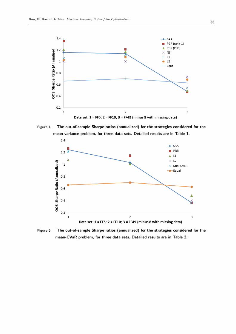
Out-of-sample Sharpe ratio Table 1 reports the out-of-sample Sharpe ratios of the eight

strategies listed in Sec. 5.1. For p = 5, the rank-1 approximation PBR performs the best, with

a Sharpe ratio of 1.3551, followed by best convex quadratic approximation PBR (1.2052), then

SAA (1.1573). For this data set, standard regularizations (L1, L2 and no short-selling) and the

equally-weighted portfolio all perform below these strategies. Similarly, for p = 10, the rank-1

approximation PBR performs the best, with a Sharpe ratio of 1.2112, followed by best convex


Out-of-Sample Performance-Based Steepest Descent (OOS-PBSD)

Initialize

Choose backtracking parameters ↵2 (0,0.5),� 2 (0,1)

Choose stepsize Div

Choose perturbation size bit2 (0,0.5)

for b 1 to k doSet U =U�b

, �U := t(U�b

�U�b

)/Div, t= 1

Compute

dSharpe(U)

dU=r

w

Sharpe(w�b

(U))>dw�b

(U)

dU

�,

where

rw

Sharpe(w�b

(U)) =((w�b

)>⌃�b

w�b

)µ�b

� (w0�b

µ)⌃�b

w�b

((w�b

)>⌃�b

w�b

)3/2

dw�b

(U)

dU=

w�b

(U)� w�b

((1� bit)U)

bit⇥U

while

Sharpe(U � t�U)<Sharpe(U)+↵t�UdSharpe(U)

dU

dot= �t

endend

Return U⇤�b

=U � t�U.

Algorithm 2: A pseudo code for the out-of-sample performance-based steepest descentalgorithm (OOS-PBSD), which is a subroutine of (OOS-PBCV).

quadratic approximation PBR (1.1696), then SAA (1.1357); the other strategies again relatively

under perform.

The p = 41 data set yields results that are quite di↵erent from those of p = 5 and p = 10,

evidencing that dimensionality (i.e., the number of assets) is a significant factor in its own right

(this has been observed in other studies, e.g., Jagannathan and Ma (2003) and El Karoui (2010),

Karoui (2013).). While we could rank the strategies by their average out-of-sample performances,

they are statistically indistinguishable at the 5% level from the SAA method (all p-values are quite

large, the smallest being 0.3178). Hence we cannot make any meaningful conclusions for this data

set, and we leave the study of regularizing for dimensionality to future work.


From the perspective of an investor looking at the results of Table 2, the take-away is clear:

focus on a small number of assets (the Fama-French 5 Industry portfolio) and optimize using the

PBR method on both the objective and mean constraints to achieve the highest Sharpe ratio.

Portfolio turnover Table 3 reports the out-of-sample Sharpe ratios of the eight strategies

listed in Sec. 5.1. For obvious reasons, the equally-weighted portfolio achieves the smallest portfolio

turnover. For all three data sets, we find that the two PBR approximations generally have greater

portfolio turnovers than SAA, whereas the standard regularization methods (L1, L2 and no short-

selling) have lower turnovers than SAA. This is reflective of the fact that standard regularization

is by design a solution stabilizer, whereas PBR is not.

5.6. Discussion of Results: mean-CVaR problem

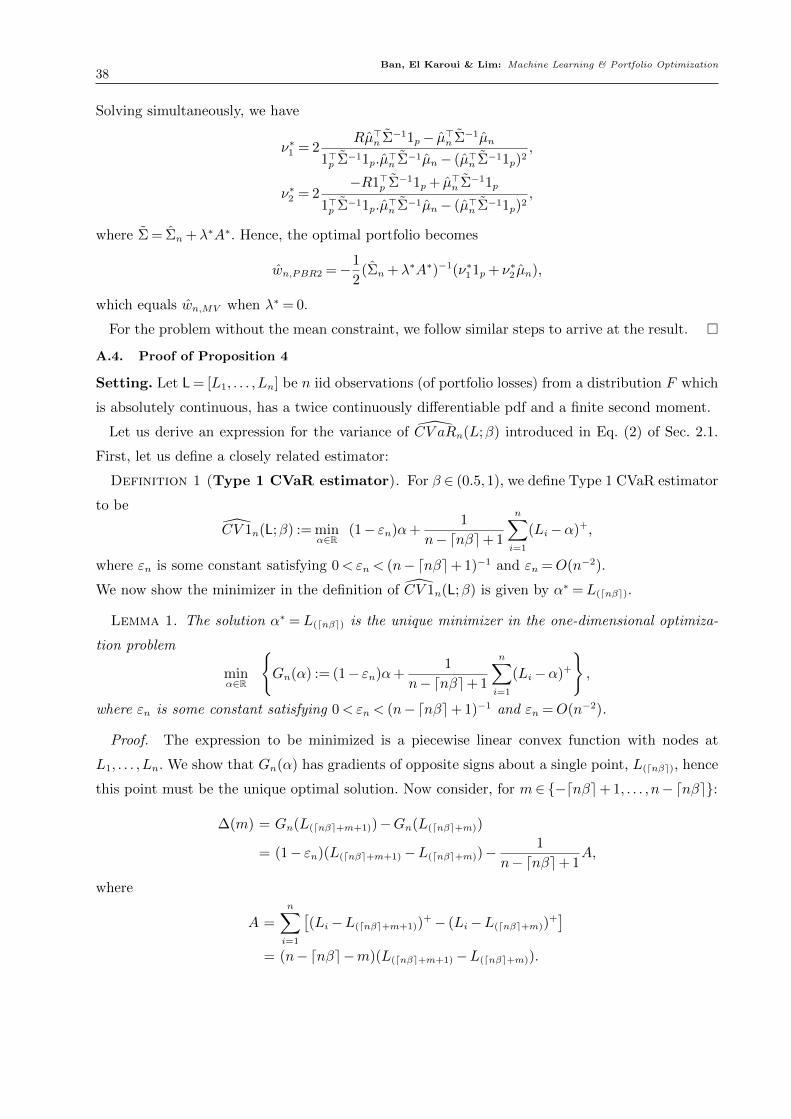
Out-of-sample Sharpe ratio Table 2 reports the out-of-sample Sharpe ratios of the eight

strategies listed in Sec. 5.2. For p= 5 and p= 10 data sets, we find that PBR on both the objective

and the constraint dominate the SAA solution. For example, the best Sharpe ratio for p= 5 for

the SAA method is achieved by setting a return target of R = 0.08, yielding a Sharpe ratio of

1.2487, whereas the best PBR result for the same data set and target return has a Sharpe ratio

of 1.2715, the di↵erence of which is statistically significant at the 5% level (the exact p-value is

0.0453). Likewise, for p= 10, the best SAA Sharpe ratio of 1.0346 is dominated by the best PBR

Sharpe ratio of 1.1506. This di↵erence is statistically significant at the 10% level (the exact p-value

is 0.0607). Also for p= 5 and p= 10 data sets, the PBR method consistently dominates both L1

and L2 regularizations across all problem target returns and choice of the number of bins used for

cross validation. In addition, both the equally-weighted portfolio and the global minimum CVaR

portfolios underperform SAA, hence also PBR on these data sets.

The p= 41 data set yields results that are quite di↵erent from those of p= 5 and p= 10, signaling

that dimensionality is an important parameter in its own right. First of all, the highest Sharpe ratio

of all strategies across all target return levels and choice of bins is achieved by the equally-weighted

portfolio, with 0.6297. Secondly, all regularizations — PBR, L1 and L2 — yield results that are

statistically indistinguishable from the SAA method (all p-values are quite large, the smallest being

0.6249). Hence we cannot make any meaningful conclusions for this data set, and we leave the

study of regularizing for dimensionality to future work.

Lastly, let us comment on the e↵ects of PBR on the objective and the mean estimations sep-

arately. The question that comes to mind is whether one constraint dominates the other; i.e.,

whether PBR on the objective only consistently dominates PBR on the mean, or vice versa. The

answer is a yes, but the exact relationship depends on the data set: for p= 5 and p= 10, the Sharpe

ratios of PBR on CVaR is better than that of PBR on the mean for each target return (and taking


the best of the two bin results), whereas for p = 41, the opposite is true. This pattern seems to

indicate that for a smaller number of assets, CVaR estimation is more of an issue whereas mean

estimation is more problematic for a larger number of assets.

Portfolio turnover Table 3 reports the out-of-sample Sharpe ratios of the eight strategies

listed in Sec. 5.2. For obvious reasons, the equally-weighted portfolio achieves the smallest portfolio

turnover. For the p = 5 data set, the PBR method is consistently lower than SAA, L1 and L2

regularization methods for each target return level and across the two bins sizes considered. The

opposite is true for p= 10 or p= 41 however, with PBR having consistently higher turnovers than

SAA, L1 and L2 regularization methods for each target return level and across the two bins sizes

considered. Global minimum variance portfolios have turnovers greater than the equally-weighted

portfolio but generally less than the SAA method.

6. Conclusion

We introduced performance-based regularization and performance-based cross-validation for the

portfolio optimization problem and investigated them in detail. The PBR models constrain sample

variances of estimated quantities in the problem, namely the portfolio risk and return. The PBR

models are shown to have equivalent robust counterparts, with new, non-trivial robust constraints

for the portfolio risk. We have shown that PBR with performance-based cross-validation is highly

e↵ective at improving the finite-sample performance of the data-driven portfolio decision compared

to SAA as well as other benchmarks known benchmarks in the literature. We conclude that PBR is

a promising modeling paradigm for handling uncertainty, and worthy of further study to generalize

to other decision problems.


Table 1 Sharpe Ratios for empirical data for the mean-variance problem.

FF 5 Industry FF 10 Industry FF 49 Industryp=5 p=10 p=41

(-8 assets with missing data)Mean-Variance R=0.04

SAA 1.1459 1.1332 0.47442 bins 3 bins 2 bins 3 bins 2 bins 3 bins

PBR (rank-1) 1.2603 1.3254 1.1868 1.2098 0.4344 0.4712(0.0411) (0.0286) (0.0643) (0.0509) (0.5848) (0.5386)

PBR (PSD) 1.1836 1.1831 1.1543 1.1678 0.4776 0.4825(0.0743) (0.071) (0.0891) (0.0816) (0.5593) (0.5391)

NS 1.0023 0.9968 0.7345(0.1404) (0.1437) (0.2977)

L1 1.0136 1.0386 1.1185 1.1175 0.5419 0.5211(0.1568) (0.1396) (0.1008) (0.1017) (0.5044) (0.5216)

L2 0.9711 1.0268 1.0579 1.0699 0.6672 0.6009(0.1781) (0.1452) (0.1482) (0.1280) (0.3950) (0.4455)

Mean-Variance R=0.06SAA 1.1535 1.1357 0.4468

2 bins 3 bins 2 bins 3 bins 2 bins 3 binsPBR (rank-1) 1.2945 1.3362 1.1870 1.2112 0.4011 0.4515

(0.0297) (0.0244) (0.0629) (0.0503) (0.6136) (0.5530)PBR (PSD) 1.1912 1.2052 1.1532 1.1696 0.4585 0.4587

(0.0689) (0.0638) (0.0898) (0.0809) (0.5757) (0.5598)NS 0.9853 0.9699 0.7124

(0.1422) (0.1537) (0.3247)L1 0.9963 1.0198 1.0902 1.1010 0.4991 0.4941

(0.1535) (0.1394) (0.1124) (0.1101) (0.5490) (0.5448)L2 0.9713 1.0265 1.0642 1.0755 0.6313 0.5701

(0.1735) (0.1425) (0.1425) (0.1238) (0.4250) (0.4696)Markowitz R=0.08


PBR (rank-1) 1.3286 1.3551 1.1743 1.2018 0.3927 0.4253(0.0223) (0.0208) (0.0668) (0.0510) (0.6142) (0.5778)

PBR (PSD) 1.1813 1.1952 1.1467 1.1575 0.4477 0.4366(0.0648) (0.0614) (0.0893) (0.0844) (0.5852) (0.5804)

NS 0.9664 0.9405 0.6600(0.1514) (0.1577) (0.3790)

L1 0.9225 0.9965 1.0318 1.0779 0.4770 0.4930(0.1857) (0.1403) (0.1332) (0.1181) (0.5649) (0.5379)

L2 0.9703 1.0284 1.0671 1.0776 0.6098 0.5522(0.1649) (0.1398) (0.1398) (0.1209) (0.4369) (0.4785)

Min. VarianceSAA 1.1454 1.1331 0.4816

2 bins 3 bins 2 bins 3 bins 2 bins 3 binsPBR (rank-1) 1.2580 1.3269 1.1922 1.2086 0.4409 0.4683

(0.0420) (0.0288) (0.0603) (0.0505) (0.5795) (0.5472)PBR (PSD) 1.1883 1.1882 1.154 1.1657 0.4942 0.4903

(0.0710) (0.0693) (0.0892) (0.0823) (0.5400) (0.5322)NS 1.0022 1.0012 0.7347

(0.1405) (0.1447) (0.3178)L1 1.0321 1.0546 1.1199 1.1111 0.5424 0.5260

(0.1455) (0.1286) (0.1000) (0.1026) (0.5017) (0.5151)L2 0.9945 1.0140 1.0543 1.0760 0.6886 0.6204

(0.1632) (0.1472) (0.1488) (0.1236) (0.3761) (0.4276)Equal 0.6617 0.7019 0.6297

This table reports the annualized out-of-sample Sharpe ratios of solutions to the mean-variance problem solved with

the methods described in Sec. 5.1 for three di↵erent data sets for target returns R= 0.04,0.06,0.08. For each data set,

the highest Sharpe ratio attained by each strategy is highlighted in boldface. To set the degree of regularization, weuse the performance-based k-fold cross validation algorithm detailed in Sec. 5.4, with k= 2 and 3 bins. In parentheses

we report the p-values of tests of di↵erences from the SAA method. We also report the Sharpe ratio of the equally-

weighted portfolio.


Table 2 Sharpe Ratios for empirical data for the mean-CVaR problem.


(-8 assets with missing data)Mean-CVaR R=0.04


PBR (CVaR only) 1.2113 1.1733 1.0506 1.1381 0.1304 0.1304(0.0554) (0.0674) (0.0638) (0.0312) (0.7908) (0.7908)

PBR (mean only) 1.2089 1.1802 1.0994 1.0519 0.2732 0.3682(0.0746) (0.0790) (0.1051) (0.1338) (0.7518) (0.6454)

PBR (both) 1.2439 1.2073 1.1112 1.1422 0.3607 0.2247(0.0513) (0.0601) (0.0691) (0.0648) (0.7054) (0.7667)

L1 1.0112 1.0754 0.9254 0.9741 0.4048 0.4642(0.1497) (0.1366) (0.2293) (0.1880) (0.6874) (0.6242)

L2 0.9650 1.0636 1.0031 0.9835 0.3982 0.3586(0.1780) (0.1287) (0.1512) (0.1598) (0.7087) ( 0.6878)

Mean-CVaR R=0.06SAA 1.2179 1.0321 0.3657

2 bins 3 bins 2 bins 3 bins 2 bins 3 binsPBR (CVaR only) 1.2223 1.2063 1.0518 1.1451 0.1265 0.1300

(0.0503) (0.0527) (0.0633) (0.0294) (0.7920) (0.7909)PBR (mean only) 1.2205 1.1902 1.0988 1.0466 0.2704 0.3771

(0.0699) (0.0746) (0.1053) (0.1358) (0.7531) (0.6359)PBR (both) 1.2450 1.2043 1.1122 1.1506 0.3503 0.2267

(0.0504) (0.0581) (0.0686) (0.0607) (0.7102) (0.7656)L1 0.9404 1.0464 0.9276 0.9746 0.3888 0.4635

(0.1812) (0.1395) (0.2282) (0.1887) (0.7001) (0.6249)L2 0.9271 1.0627 1.0146 0.9794 0.3842 0.3571

(0.1977) (0.1286) (0.1432) (0.1621) (0.7175) (0.6886)Mean-CVaR R=0.08


PBR (CVaR only) 1.2493 1.2098 1.0551 1.1433 0.1304 0.1304(0.0434) (0.0462) (0.0579) (0.0323) (0.7908) (0.7908)

PBR (mean only) 1.2480 1.2088 1.0987 1.0470 0.2675 0.3738(0.0591) (0.0693) (0.1053) (0.1384) (0.7541) (0.6391)

PBR (both) 1.2715 1.2198 1.1122 1.1449 0.2656 0.2285(0.0453) (0.0544) (0.0664) (0.0639) (0.7618) (0.7647)

L1 0.8921 0.9836 0.9416 1.0087 0.3855 0.4872(0.1964) (0.1572) (0.2122) (0.1645) (0.7008) (0.6128)

L2 0.9367 1.0801 1.0278 0.9947 0.3784 0.3588(0.1989) (0.1179) (0.1323) (0.1530) (0.7177) (0.6870)

Global min. CVaR 1.2137 1.0321 0.3657Equal 0.6617 0.7019 0.6297

This table reports the annualized out-of-sample Sharpe ratios of the solutions to the mean-CVaR problem solved

with SAA, PBR with regularization of the objective (“CVaR only”), the constraint (“mean only”) and both theobjective and the constraint (“both”), L1 and L2 regularization constraints for three di↵erent data sets and for target

returns R = 0.04,0.06,0.08. For each data set, the highest Sharpe ratio attained by each strategy is highlighted in

boldface. To set the degree of regularization, we use the performance-based k-fold cross validation algorithm detailedin Sec. 5.4, with k= 2 and 3 bins. In parentheses we report the p-values of tests of di↵erences from the SAA method.

We also report the Sharpe ratio of the equally-weighted portfolio and the solution to the global minimum CVaRproblem (no mean constraint).


Table 3 Turnovers for empirical data for the mean-variance problem.


(-8 assets with missing data)Mean-Variance R=0.04


PBR (rank-1) 0.1213 0.1292 0.1746 0.1851 0.5442 0.6611PBR (PSD) 0.1002 0.0988 0.1415 0.1523 0.5201 0.4999

NS 0.0391 0.0544 0.0833L1 0.0986 0.0848 0.1158 0.1208 0.5167 0.4453L2 0.1171 0.0901 0.1255 0.1071 0.4704 0.4079


2 bins 3 bins 2 bins 3 bins 2 bins 3 binsPBR (rank-1) 0.1397 0.1357 0.1741 0.1841 0.5646 0.6427PBR (PSD) 0.1132 0.1086 0.1442 0.1513 0.5301 0.5042

NS 0.0417 0.0711 0.0859L1 0.1206 0.0963 0.1256 0.1205 0.4992 0.4439L2 0.1267 0.0992 0.1379 0.1121 0.4809 0.4110



NS 0.0511 0.0965 0.1122L1 0.1476 0.1246 0.1480 0.1392 0.5064 0.4567L2 0.1582 0.1241 0.1470 0.1229 0.5118 0.4200

Min. VarianceSAA 0.1034 0.1325 0.5146


NS 0.0391 0.0524 0.0835L1 0.0995 0.0886 0.1138 0.1219 0.4956 0.4435L2 0.1213 0.0910 0.1255 0.1061 0.4575 0.4070

Equal 0.0427 0.0382 0.0483

This table reports the portfolio turnovers (defined in Eq. 15) of the solutions to the mean-variance problem solved

with the methods described in Sec. 5.1 for three di↵erent data sets and for target returns R= 0.04,0.06,0.08. We alsoreport the turnovers of the equally-weighted portfolio.


Table 4 Turnovers for empirical data for the mean-CVaR problem.

Sharpe Ratios FF 5 Industry FF 10 Industry FF 49 Industryp=5 p=10 p=41

(-8 assets with missing data)Mean-CVaR R=0.04


PBR (CVaR only) 0.1834 0.1985 0.4049 0.5586 1.7773 1.7773PBR (mean only) 0.1230 0.1274 0.3104 0.2731 1.3173 1.5023

PBR (both) 0.1387 0.1388 0.3700 0.3682 1.7492 1.4158L1 0.1992 0.1581 0.3415 0.2722 1.5158 1.3731L2 0.1565 0.1469 0.2288 0.2270 1.2192 1.1217

Mean-CVaR R=0.06SAA 0.2909 0.3534 1.6833

2 bins 3 bins 2 bins 3 bins 2 bins 3 binsPBR (CVaR only) 0.1918 0.2074 0.4071 0.5616 1.7922 1.7778PBR (mean only) 0.1364 0.1414 0.3100 0.2729 1.3188 1.5147

PBR (both) 0.1519 0.1526 0.3724 0.3672 1.7610 1.4170L1 0.2263 0.1754 0.3498 0.2723 1.5232 1.3730L2 0.1842 0.1532 0.2407 0.2401 1.2374 1.1220

Mean-CVaR R=0.08SAA 0.2980 0.3615 1.6833

2 bins 3 bins 2 bins 3 bins 2 bins 3 binsPBR (CVaR only) 0.2148 0.2242 0.4486 0.6472 1.7775 1.7775PBR (mean only) 0.1517 0.1575 0.3066 0.2827 1.3228 1.5038

PBR (both) 0.1693 0.1681 0.4099 0.4034 1.6887 1.4190L1 0.3100 0.2395 0.3628 0.3042 1.5370 1.3731L2 0.2451 0.1835 0.2588 0.2633 1.1774 1.1227

Global min. CVaR 0.2857 0.3534 1.6833Equal 0.0427 0.0382 0.0483

This table reports the portfolio turnovers (defined in Eq. 15) of the solutions to the mean-CVaR problem solved

with SAA, PBR with regularization of the objective (“CVaR only”), the constraint (“mean only”) and both the

objective and the constraint (“both”), L1 and L2 regularization constraints for three di↵erent data sets and for targetreturns R = 0.04,0.06,0.08. We also report the turnovers of the equally-weighted portfolio and the solution to the

global minimum CVaR problem (no mean constraint).


Figure 4 The out-of-sample Sharpe ratios (annualized) for the strategies considered for the

mean-variance problem, for three data sets. Detailed results are in Table 1.

Figure 5 The out-of-sample Sharpe ratios (annualized) for the strategies considered for the

mean-CVaR problem, for three data sets. Detailed results are in Table 2.


Online Appendix:Machine Learning & Portfolio Optimization

Gah-Yi Ban, Noureddine El Karoui, Andrew E.B. Lim

Appendix A: Proofs of results in Sec. 3

A.1. Proof of Proposition 1

Let X1, . . . ,Xn be n iid observations of the vector X. We wish to compute the covariance of the

sample covariance matrix S, whose elements are:

S2ij

=

"1

n

nX

k=1

(Xk

i

� Xi

)(Xk

j

� Xj

)

#, (16)

where Xi

= 1n

Pn

k=1Xk

i

is the sample mean of the i-th element of X.

Transformation into a U-statistic For convenience, we transform (16) into a U-statistic:

S2ij

=1�n

2

�X

(k,l)

1

2(Xk

i

�X l

i

)(Xk

j

�X l

j

)

Then the variance of the ij-th element of the sample covariance matrix is given by

Cov(S2ij

,S2kl

) =E

2

4 1�n

2

�X

(p,q)

1

2(Xp

i

�Xq

i

)(Xp

j

�Xq

j

)��2ij

3

5

2

4 1�n

2

�X

(r,s)

1

2(Xr

k

�Xs

k

)(Xr

l

�Xs

l

)��2kl

3

5

=1�n

2

�2E

8<

:X

(p,q)

X

(r,s)

[1

2(Xp

i

�Xq

i

)(Xp

j

�Xq

j

)��2ij

][1

2(Xr

k

�Xs

k

)(Xr

l

�Xs

l

)��2kl

]

9=

; .

There are three cases:

1. |(k, l)\ (k0, l0)|= 0 then by independence the product is zero.

2. |(k, l)\ (k0, l0)|= 1, in other words, we have n(n� 1)(n� 2) terms of the form

[1

2(Xp

i

�Xq

i

)(Xp

j

�Xq

j

)��2ij

][1

2(Xp

k

�Xs

k

)(Xp

l

�Xs

l

)��2kl

]

Now

[1

2(Xp

i

�Xq

i

)(Xp

j

�Xq

j

)��2ij

][1

2(Xp

k

�Xs

k

)(Xp

l

�Xs

l

)��2kl

]

=1

4[Xp

i

Xp

j

�Xp

i

Xq

j

�Xq

i

Xp

j

][Xp

k

Xp

l

�Xp

k

Xs

l

�Xs

k

Xp

l

]

+1

4Xq

i

Xq

j

[Xp

k

Xp

l

�Xp

k

Xs

l

�Xs

k

Xp

l

] +1

4Xs

k

Xs

l

[Xp

i

Xp

j

�Xp

i

Xq

j

�Xq

i

Xp

j

]

+1

4Xq

i

Xq

j

Xs

k

Xs

l

� 1

2�2kl

[Xp

i

Xp

j

�Xp

i

Xq

j

�Xq

i

Xp

j

+Xq

i

Xq

j

]� 1

2�2ij

[Xp

k

Xp

l

�Xp

k

Xs

l

�Xs

k

Xp

l

+Xs

k

Xs

l

] +�2ij

�2kl

,


so taking expectations and simplifying, we get

E[12(Xp

i

�Xq

i

)(Xp

j

�Xq

j

)��2ij

][1

2(Xp

k

�Xs

k

)(Xp

l

�Xs

l

)��2kl

]

=1

4(µ4,ijkl��2

ij

�2kl

).

3. |(k, l)\ (k0, l0)|= 2, in other words, we have�n

2

�terms of the form

[1

2(Xp

i

�Xq

i

)(Xp

j

�Xq

j

)��2ij

][1

2(Xp

k

�Xq

k

)(Xp

l

�Xq

l

)��2kl

]

Now

[1

2(Xp

i

�Xq

i

)(Xp

j

�Xq

j

)��2ij

][1

2(Xp

k

�Xq

k

)(Xp

l

�Xq

l

)��2kl

]

=1

4[Xp

i

Xp

j

Xp

k

Xp

l

+Xq

i

Xq

j

Xq

k

Xq

l

]

� 1

4[Xp

i

Xp

j

Xp

k

Xq

l

+Xp

i

Xp

j

Xq

k

Xp

l

+Xp

i

Xq

j

Xp

k

Xp

l

+Xq

i

Xp

j

Xp

k

Xp

l

]

� 1

4[Xp

i

Xq

j

Xq

k

Xq

l

+Xq

i

Xp

j

Xq

k

Xq

l

+Xq

i

Xq

j

Xp

k

Xq

l

+Xq

i

Xq

j

Xq

k

Xp

l

]

+1

4[Xp

i

Xp

j

Xq

k

Xq

l

+Xp

i

Xq

j

Xp

k

Xq

l

+Xp

i

Xq

j

Xq

k

Xp

l

+Xq

i

Xp

j

Xp

k

Xq

l

+Xq

i

Xp

j

Xq

k

Xp

l

+Xq

i

Xq

j

Xp

k

Xp

l

]

� 1

2�2kl

[Xp

i

Xp

j

�Xp

i

Xq

j

�Xq

i

Xp

j

+Xq

i

Xq

j

]� 1

2�2ij

[Xp

k

Xp

l

�Xp

k

Xq

l

�Xq

k

Xp

l

+Xq

k

Xq

l

] +�2ij

�2kl

,

so taking expectations and simplifying, we get

E[12(Xp

i

�Xq

i

)(Xp

j

�Xq

j

)��2ij

][1

2(Xp

k

�Xq

k

)(Xp

l

�Xq

l

)��2kl

]

=1

2(µ4,ijkl��2

ij

�2kl

+�2ik

�2jl

+�2il

�2jk

).

Putting it all together,

Cov(S2ij

,S2kl

) =1

n(µ4,ijkl��2

ij

�2kl

)+1

n(n� 1)(�2

ik

�2jl

+�2il

�2jk

). (17)


Let us start with (mv-PBR-1) with the mean constraint. The Lagrangian is:

L(w;⌫1,⌫2,�) =w>⌃n

w+ ⌫1(w>1

p

� 1)+ ⌫2(w>µ

n

�R)+�(w>↵� 4pU)

=w>⌃n

w+w>(⌫11p + ⌫2µn

+�↵)� ⌫1� ⌫2R��4pU

The first order condition (FOC) gives:

w⇤ =�1

2⌃�1

n

(⌫11p + ⌫2µn

+�↵) (18)


The Lagrangian dual function is:

g(⌫1,⌫2,�) = infw

L(w;⌫1,⌫2,�)

=�1

4(⌫11p + ⌫2µn

+�↵)>⌃�1n

(⌫11p + ⌫2µn

+�↵)� ⌫1� ⌫2R��4pU

At optimality, g is maximized over (⌫1,⌫2,�)2Rp⇥Rp⇥R+. We will maximize g over (⌫1,⌫2) first.

The first order conditions give:

dg(⌫1,⌫2,�)

d⌫1=�1

2(⌫2µn

+�↵)>⌃�1n

1p

� 1

2⌫11

>p

⌃�1n

1p

� 1 = 0

dg(⌫1,⌫2,�)

d⌫2=�1

2(⌫11p +�↵)>⌃�1

n

µn

� 1

2⌫2µ

>n

⌃�1n

µn

�R= 0.

Solving simultaneously, we have

⌫⇤1 = 2

µ>n

⌃�1n

µn

�Rµ>n

⌃�1n

1p

1>p

⌃�1n

1p

.µ>n

⌃�1n

µn

� (µ>n

⌃�1n

1p

)2+�

↵>⌃�1n

µn

.µ>n

⌃�1n

1p

� ↵>⌃�1n

1p

.µ>n

⌃�1n

µn

1>p

⌃�1n

1p

.µ>n

⌃�1n

µn

� (µ>n

⌃�1n

1p

)2= ⌫0

1 +��1

⌫⇤2 = 2

1>p

⌃�1n

µn

�R1>p

⌃�1n

1p

1>p

⌃�1n

1p

.µ>n

⌃�1n

µn

� (µ>n

⌃�1n

1p

)2+�

↵>⌃�1n

µn

.1>p

⌃�1n

1p

� ↵>⌃�1n

1p

.1>p

⌃�1n

µn

1>p

⌃�1n

1p

.µ>n

⌃�1n

µn

� (µ>n

⌃�1n

1p

)2= ⌫0

2 +��2,

where ⌫01 ,⌫

02 are optimal dual variables for the original mean-variance problem. Hence, the optimal

portfolio becomes

wn,PBR1 =�

1

2⌃�1

n

((⌫01 +��1)1p +(⌫0

2 +��2)µn

+�↵)

=�1

2⌃�1

n

(⌫011p + ⌫0

2 µn

)� 1

2�⌃�1

n

(�11p +�2µn

+ ↵)

= wn,MV

� 1

2�⌃�1

n

(�11p +�2µn

+ ↵),

where wn,MV

is the optimal portfolio of the SAA mean-variance problem without PBR.

For the problem without the mean constraint, we follow similar steps. The Lagrangian is:

L(w;⌫,�) =w>⌃n

w+ ⌫(w>1p

� 1)+�(w>↵� 4pU)

=w>⌃n

w+w>(⌫1p

+�↵)� ⌫��4pU

The FOC gives:

w⇤ =�1

2⌃�1

n

(⌫1p

+�↵) (19)


g(⌫,�) = infw

L(w;⌫,�)

=�1

4(⌫1

p

+�↵)>⌃�1n

(⌫1p

+�↵)� ⌫��4pU,


and

dg(⌫,�)

d⌫=�1

2�↵>⌃�1

n

1p

� 1

2⌫1>

p

⌃�1n

1p

� 1 = 0

Solving for ⌫, we get

⌫⇤ =� 2

1>p

⌃�1n

1p

��1>p

⌃�1n

↵

1>p

⌃�1n

1p

= ⌫0 +��

where ⌫0 is the optimal dual variables for the SAA mean-variance problem without the mean

constraint. Hence, the optimal portfolio becomes

wn,PBR1 =�

1

2⌃�1

n

((⌫0 +��)1p

+�↵)

=�1

2⌫0⌃�1

n

1p

� 1

2�⌃�1

n

(�1p

+ ↵)

= wn,MV

� 1

2�⌃�1

n

(�1p

+ ↵)

where wn,MV

is the optimal portfolio of the SAA mean-variance problem without PBR. ⇤


Let us start with (mv-PBR-2) with the mean constraint. The Lagrangian is:

L(w;⌫1,⌫2,�) =w>⌃n

w+ ⌫1(w>1

p

� 1)+ ⌫2(w>µ

n

�R)+�(w>A⇤w�pU)

=w>(⌃n

+�A⇤)w+w>(⌫11p + ⌫2µn

)� ⌫1� ⌫2R��pU

The FOC gives:

w⇤ =�1

2(⌃

n

+�A⇤)�1(⌫11p + ⌫2µn

) (20)


g(⌫1,⌫2,�) = infw

L(w;⌫1,⌫2,�)

=�1

4(⌫11p + ⌫2µn

)>(⌃n

+�A⇤)�1(⌫11p + ⌫2µn

)� ⌫1� ⌫2R��pU

At optimality, g is maximized over (⌫1,⌫2,�)2Rp⇥Rp⇥R+. We will maximize g over (⌫1,⌫2) first.

The first order conditions give:

dg(⌫1,⌫2,�)

d⌫1=�1

2⌫2µ

>n

(⌃n

+�A⇤)�11p

� 1

2⌫11

>p

(⌃n

+�A⇤)�11p

� 1 = 0

dg(⌫1,⌫2,�)

d⌫2=�1

2⌫11

>p

(⌃n

+�A⇤)�1µn

� 1

2⌫2µ

>n

(⌃n

+�A⇤)�1µn

�R= 0.


Solving simultaneously, we have

⌫⇤1 = 2

Rµ>n

⌃�11p

� µ>n

⌃�1µn

1>p

⌃�11p

.µ>n

⌃�1µn

� (µ>n

⌃�11p

)2,

⌫⇤2 = 2

�R1>p

⌃�11p

+ µ>n

⌃�11p

1>p

⌃�11p

.µ>n

⌃�1µn

� (µ>n

⌃�11p

)2,

where ⌃= ⌃n

+�⇤A⇤. Hence, the optimal portfolio becomes

wn,PBR2 =�

1

2(⌃

n

+�⇤A⇤)�1(⌫⇤11p + ⌫⇤

2 µn

),

which equals wn,MV

when �⇤ = 0.

For the problem without the mean constraint, we follow similar steps to arrive at the result. ⇤A.4. Proof of Proposition 4

Setting. Let L= [L1, . . . ,Ln

] be n iid observations (of portfolio losses) from a distribution F which

is absolutely continuous, has a twice continuously di↵erentiable pdf and a finite second moment.

Let us derive an expression for the variance of \CV aRn

(L;�) introduced in Eq. (2) of Sec. 2.1.

First, let us define a closely related estimator:

Definition 1 (Type 1 CVaR estimator). For � 2 (0.5,1), we define Type 1 CVaR estimator

to be

[CV 1n

(L;�) :=min↵2R

(1� "n

)↵+1

n�dn�e+1

nX

i=1

(Li

�↵)+,

where "n

is some constant satisfying 0< "n

< (n�dn�e+1)�1 and "n

=O(n�2).

We now show the minimizer in the definition of [CV 1n

(L;�) is given by ↵⇤ =L(dn�e).

Lemma 1. The solution ↵⇤ = L(dn�e) is the unique minimizer in the one-dimensional optimiza-

tion problem

min↵2R

(G

n

(↵) := (1� "n

)↵+1

n�dn�e+1

nX

i=1

(Li

�↵)+),

where "n

is some constant satisfying 0< "n

< (n�dn�e+1)�1 and "n

=O(n�2).

Proof. The expression to be minimized is a piecewise linear convex function with nodes at

L1, . . . ,Ln

. We show that Gn

(↵) has gradients of opposite signs about a single point, L(dn�e), hence

this point must be the unique optimal solution. Now consider, for m2 {�dn�e+1, . . . , n�dn�e}:

�(m) = Gn

(L(dn�e+m+1))�Gn

(L(dn�e+m))

= (1� "n

)(L(dn�e+m+1)�L(dn�e+m))�1

n�dn�e+1A,

where

A =nX

i=1

⇥(L

i

�L(dn�e+m+1))+� (L

i

�L(dn�e+m))+⇤

= (n�dn�e�m)(L(dn�e+m+1)�L(dn�e+m)).


Thus

�(m) =�L(dn�e+m+1)�L(dn�e+m)

�✓(1� "

n

)� n�dn�e�m

n�dn�e+1

◆.

Now �(0) > 0 since (L(dn�e+1) � L(dn�e)) > 0 and (1 � "n

) > (n � dn�e)(n � dn�e + 1)�1 by the

restriction on "n

, and �(�1)< 0 since (L(dn�e)�L(dn�e�1))> 0 and (1�"n

)< 1 again by the choice

of "n

. Thus Gn

(↵) has a unique minimum at ↵⇤ =L(dn�e). ⇤Now consider the following CVaR estimator, expressed without the minimization:

Definition 2 (Type 2 CVaR estimator). For � 2 (0.5,1), we define Type 2 CVaR estimator

to be

[CV 2n

(L;�) :=1

n�dn�e+1

nX

i=1

Li

1(Li

� ↵n

(�)),

where ↵n

(�) :=L(dn�e), the dn�e-th order statistic of the sample L1, . . . ,Ln

.

The Type 2 CVaR estimator is an intuitive representation of CVaR because it is precisely the

sample average of the top (1� �) portion of the losses. Another advantage of the Type 2 CVaR

estimator is that one can write down an explicit expression for its variance. For the rest of this

subsection, our goal is to show that the Type 2 CVaR estimator is approximately equal to the

Type 1 CVaR estimator, which is in turn approximately equal to the actual CVaR estimator we

use in mean-CVaR portfolio optimization. The proof of Proposition 4 then follows.

Lemma 2. Type 1 and Type 2 CVaR estimators are related by

[CV 2n

(L;�) = [CV 1n

(L;�)+ "n

L(dn�e).

Proof. Rewriting Type 2 CVaR estimator:

[CV 2n

(L;�) =1

n�dn�e+1

nX

i=1

Li

1(Li

�L(dn�e))

= L(dn�e) +1

n�dn�e+1

nX

i=1

(Li

�L(dn�e))1(Li

�L(dn�e))

= [CV 1n

(L;�)+ "n

L(dn�e),

where the final equality is due to Lemma 1. ⇤We now prove Proposition 4.

Let ↵1n

and ↵n

be the minimizers in the definition of [CV 1n

(L;�) and \CV aRn

(L;�) respectively.

We can show, by elementary arguments,

| \CV aRn

(L;�)�[CV 1n

(L;�)| "n

(↵1n

_↵n

).


Hence we have

\CV aRn

(L;�) = [CV 1n

(L;�)+Op

("n

)

=1

n�dn�e+1

nX

i=1

Li

1(Li

�L(dn�e))+Op

("n

) by Lemma 2,

which implies

V ar[ \CV aRn

(L;�)] =1

n(1��)2V ar[L

i

1(Li

�L(dn�e))] +O(n�2),

where the O(n�2) error comes from having approximated n�dn�e+1 by n(1��) in the denomi-

nator and since "n

=O(n�2). ⇤A.5. Proof of Theorem 1

Before proving Theorem 1, we first show the following proposition.

Proposition 7. Consider the optimization problem

minz2Rn

z>1n

s.t. zi

� 0 8 izi

� ci

8 iz>⌦

n

z f

(21)

where c2Rn is some constant vector, f > 0 is a constant scalar and ⌦n

= (n�1)�1(In

�n�11n

1>n

),

the sample covariance operator. Suppose (21) is feasible with an optimal solution (z⇤). Let S1(z) :=

{1 i n : zi

= 0}, S2(z) := {1 i n : zi

= ci

} and V (z) := Sc

1(z) \ Sc

2(z) = {1 i n : zi

>

max(0, ci

)}. Then, at the optimal solution z⇤, we cannot have both S1(z⇤) and V (z⇤) nonempty

simultaneously.

Proof. Problem (21) is a convex optimization problem because ⌦n

is a positive semidefinite

matrix. The problem is also strictly feasible, since z0 = 2maxi

{ci

}1n

is a strictly feasible point:

clearly, z0,i >max{0, ci

} 8 i and z>0 ⌦n

z0 = 0< f as 1n

is orthogonal to ⌦n

. Thus Slater’s condition

for strong duality holds, and we can derive properties of the optimal solution by examining the

KKT conditions.

The Lagrangian is

L(z,⌘1,⌘2,�) = �z>⌦n

z+(1n

� ⌘1� ⌘2)>z+ ⌘>

2 c��f

The KKT conditions are

• Primal feasibility

• Dual feasibility: ⌘⇤1 ,⌘

⇤2 � 0 component-wise and �⇤ � 0

• Complementary slackness:

z⇤i

⌘⇤1,i = 0 8 i, (z⇤

i

� ci

)⌘⇤2,i = 0 8 i and �⇤[(z⇤)>⌦

n

z⇤� f ] = 0


• First Order Condition:

rz

⇤L = 2�⌦n

z⇤ +(1n

� ⌘⇤1 � ⌘⇤

2) = 0 (22a)

By substituting for ⌦n

, (22a) can be written as

2�

n� 1

✓z⇤� 1

n(1>

n

z⇤)1n

◆= �1

n

+ ⌘⇤1 + ⌘⇤

2 . (23)

Suppose S1(z⇤) 6= ; at the optimal primal-dual point (z⇤,⌘⇤1 ,⌘

⇤2 ,�

⇤). Then 9 i0 2 S1(z⇤) such that

z⇤i0= 0. The i0-th component of (23) gives

� 2�⇤

n(n� 1)(1>

n

z⇤) = �1+ ⌘⇤1,i0

+ ⌘⇤2,i0

. (24)

Now suppose V (z⇤) 6= ; at the optimal primal-dual point (z⇤,⌘⇤1 ,⌘

⇤2 ,�

⇤). Then 9 j0 2 V (z⇤) such

that z⇤j0>max(0, c

i

), which implies ⌘⇤1,j0

= 0 and ⌘⇤2,j0

= 0 by complementary slackness. The j0-th

component of (23) gives

2�⇤

n� 1

✓z⇤j0� 1

n(1>

n

z⇤)

◆= �1, (25)

which implies �⇤ > 0 since �⇤ cannot equal zero.

Now suppose S1(z⇤) and V (z⇤) are both nonempty. Combining (24) and (25), we arrive at the

necessary condition2�⇤

n� 1z⇤j0=�⌘⇤

1,i0� ⌘⇤

2,i0.

which is clearly a contradiction since lhs > 0 whereas rhs 0. Hence S1(z⇤) and V (z⇤) cannot both

be nonempty, and the result follows. ⇤We now prove Theorem 1.

Clearly, (cv-relax) is a relaxation of (cv-PBR0): the components of the variable z in (cv-relax)

are relaxations of max(0,�w>Xi

� ↵). Thus the two problem formulations are equivalent if at

optimum, zi

=max(0,�w>Xi

�↵) 8 i= 1, . . . , n for (cv-relax).

Let (↵⇤,w⇤, z⇤,⌫⇤1 ,⌫

⇤2 ,⌘

⇤1 ,⌘

⇤2 ,�

⇤1,�

⇤2) be the primal-dual optimal point for (cv-relax) and (cv-relax-

d). Our aim is to show that V (z⇤), the set of indices for which z⇤i

>max(0,�w>Xi

�↵), is empty.

Suppose the contrary. Then by Proposition 7, S1(z⇤), the set of indices for which z⇤i

= 0, is empty.

This means z⇤i

> 0 8 i and ⌘⇤1,i = 0 8 i by complementary slackness.

Now consider the sub-problem for a fixed ⌘2 in the dual problem (cv-relax-d):

max⌘1:⌘1�0

� (⌘1 + ⌘2)⌦†n

(⌘1 + ⌘2). (26)

As 1n

is orthogonal to ⌦†n

, and ⌦†n

is positive semidefinite, the optimal solution is of the form

⌘1 = a1n

� ⌘2, where a is any constant such that a � maxi

(⌘2,i), with a corresponding optimal

objective 0. Hence, bearing in mind the constraints ⌘2 � 0 and ⌘>2 1n = 1 in (cv-relax-d), ⌘1 = 0 is

one of the optimal solutions i↵ ⌘⇤2 = 1

n

/n. Thus if ⌘⇤2 6= 1

n

/n, we get a contradiction. Otherwise, we

can force the dual problem to find a solution with ⌘1 6= 0 by introducing an additional constraint

⌘>1 1n � � for some constant 0< �< 1 in the dual problem (cv-relax-d). ⇤



The lhs of the RO constraint in (mv-PBR-RO) is equivalent to the convex optimization problem

minu2Rp:(I�PP

†)u=0�w>u

s.t. u>P�†u 1(RO constraint)

The Lagrangian is

L(u,�) =�w>u+�u>P †u��,

with

ru

L(u,�) =�w+2�P †u,

which equals zero for P †u⇤ = 12�w, i.e., when

u⇤ = u⇤(!) =1

2�Pw+(I �PP †)!,

for arbitrary ! 2Rp. However, the condition (I �PP †)u= 0 implies

1

2�(I �PP †)Pw+(I �PP †)2!=

1

2�(P �PP †P )w+(I �PP †)2!= (I �PP †)2!= 0,

since PP †P = P . If P is invertible, the above is trivially satisfied because (I � PP †) is the zero

matrix, and if P is not invertible then ! is restricted to be orthogonal to (I�PP †). In either case,

(I �PP †)!= 0, and u⇤ = 12�Pw.

Thus the dual function is

g(�) =L(u⇤(!),�) =� 1

4�w>Pw��,

with

dg(�)

d�=

1

4�2w>Pw� 1,

which equals zero for �⇤ = 12

pw>Pw. Substituting this value into the dual function, we get

�pw>Pw. Thus the RO constraint is equal to

pw>Pw 4

pU,

and substituting P = ↵↵> for (mv-PBR-1) and P =A⇤ for (mv-PBR-2) we obtain the PBR con-

straints. ⇤


Appendix B: PBR is di↵erent from known robust optimization models

In this section, we show that the PBR constraints on the portfolio risk are not equivalent to known

robust optimization constraints such as those found in Delage and Ye (2010).

Case I: mean-variance problem. Consider the set

A(U,�) := {w : max||⌃�⌃n||�

w>⌃wU, w>1p

= 1}

and the set

B(U 0) := {w : Svar(w>⌃n

w)U 0, w>1p

= 1}.

We will show that no constants (U,�) and U 0 can make the two sets equivalent. For ease of

exposition, let us consider the single asset (p= 1) case. Clearly, the wealth sum constraint implies

w= 1 in this case.

The robust constraint of set A(U,�) is then given by

max|�2��

2n|�

�2 U

() max�

2n��

2�

2n+�

�2 U

() �2n

U � �

Thus

A(U,�) =

({1} if �2

n

U � �

; otherwise

Now the PBR constraint in set B(U 0) is given by, using the result from Proposition 1,

Svar(w2�2n

) =w4

1

n(µ4,n� �4

n

)+2

n(n� 1)�4n

�U 0,

where µ4,n is the sample estimate for the fourth central moment of the asset return distribution.

When w= 1, the above equals1

nˆµ4,n +

3�n

n(n� 1)�4n

U 0,

thus

B(U 0) =

({1} if 1

n

µ4,n +3�n

n(n�1)�4n

U 0

; otherwise.

It is thus clear that no choice of (U,�) and U 0 would make the two sets equivalent, unless there is

a particular relationship between the sample variance and the fourth central moment of the asset

return distribution. It is also clear that the main di↵erence between the two sets is that the PBR


set B(U 0) involves fourth moments of the asset return distribution, because it penalizes uncertainty

in the risk estimation, whereas the standard robust constraint only involves the second moment

of the asset return distribution because the robust protection is against the range of the second

moment directly, rather than the whole risk function.

Case II: mean-CVaR problem. Consider the set

A(U,�) :=

(w : max

||q�qn||�

↵+1

1��

nX

i=1

qi

(�wi

�↵)+ U, w>1p

= 1

),

where qi,n

= 1/n, the empirical measure, and the norm on the measure q is the total variational

distance, and the set

B(U 0) :=

⇢w :

1

n(1��)2z>⌦

n

z U 0, w>1p

= 1, zi

= (�wi

�↵)+, i= 1, . . . , n

�

=

(w :

1

n(n� 1)(1��)2

nX

i=1

(zi

� zn

)U 0, w>1p

= 1, zi

= (�wi

�↵)+, i= 1, . . . , n

)

where zn

is the sample mean of z1, . . . , zn.

As before, we will show that no constants (U,�) and U 0 can make the two sets equivalent. By

the equivalence of the total variational distance to the 1-norm for a discrete distribution,

||q� qn

||= 1

2

nX

i=1

��qi

� 1

n

��,

and since the term multiplying qi

’s are all non-negative, the optimal q, gives all weight to the

largest (�wi

�↵)+ term, i.e.,

max||q�qn||�

↵+1

1��

nX

i=1

qi

(�w>Xi

�↵)+ = ↵+1

1��

✓1

n+2�

◆max

i

(�wi

�↵)+,

and so

A(U,�) =

⇢w : ↵+

1

1��

✓1

n+2�

◆max

i

(�wi

�↵)+ U, w>1p

= 1

�.

Clearly, no choice of (U,�) and U 0 can make A(U,�) equivalent to B(U 0).

Appendix C: Proofs of results in Sec. 4

We prove Theorem 3 first then Theorem 2.

Proof of Theorem 3. The theory of M-estimation concerns the following scenario. Consider the

parametric function m✓

:X 7! R, where ✓ is a parameter chosen from ⇥, and X is a subset of the

Euclidean space. We are interested in finding the parameter ✓⇤ that maximizes (for minimization,

we can use �m✓

instead) the expected value of this function M(✓) = Em✓

(X), where X is drawn

from the probability space (⌦,F , P ). In the absence of the true distributional knowledge, but

in the presence of iid observations X1, . . . ,Xn

, one can estimate ✓⇤ by minimizing instead the


empirical function Mn

(✓) = n�1P

n

i=1m✓

(Xi

). Of central importance is whether the solution (or, a

near-optimal solution) to the empirical problem is consistent, i.e., whether it converges to the true

optimal as the number of observations tend to infinity. The following theorem provides su�cient

conditions for asymptotic optimality. ⇤

Theorem 5 (Theorem 5.7 in Van der Vaart (2000)). Let M,Mn

,⇥,✓⇤ be as defined in the

paragraph above, and let ✓n

be a near-optimal maximizer of Mn

, i.e.,

Mn

(✓n

)�Mn

(✓⇤)� oP

(1).

If

1. sup✓2⇥ |M

n

(✓)�M(✓)| P! 0, and

2. For all "> 0, sup✓2⇥{M(✓) : d(✓,✓⇤)� "}<M(✓⇤),

then ✓n

P! ✓⇤ as n!1.

Note 2 is true if M is continuous and ✓⇤ is unique. Also, the theorem does not require that the

estimated solution ✓n

be unique in any way; it holds for any sequence of estimated solutions.

We thus need to show the uniform convergence of Mn

(·) to M(·). By Theorem 19.4 of Van der

Vaart (2000), it su�ces to show the function class F = {m✓

: ✓ 2⇥} has a finite bracketing number

N[ ](✏,F ,L1(P )) for every ✏> 0. Without loss of generality, let us assume ⇥= [�K,K]p, where K

is a large positive scalar4.

One class of functions with a finite bracketing number is the Lipschitz class of functions, which

we define below.

Definition 3 (Lipschitz class). Consider a class of measurable functions F = {f✓

: ✓ 2 ⇥},

f✓

: X ! R, under some probability measure P . We say F is a Lipschitz class about ✓0 2 ⇥ if

✓ 7! f✓

(x) is di↵erentiable at ✓0 for P-almost every x with derivative f✓0(x) and such that, for every

✓1 and ✓2 in a neighborhood of ✓0, there exists a measurable function f with E[f2(X1)]<1 such

that

|f✓1(x)� f

✓2(x)| f(x)||✓1� ✓2||2.

Example 19.7 of Van der Vaart (2000) shows that if F = {f✓

: ✓ 2 ⇥} is a class of measurable

functions with bounded ⇥⇢Rd and F is Lipschitz about ✓0 2⇥ then for every 0< "< diam(⇥),

there exists C such that

N[ ]("qE(|f(X)|2),F ,L2(P ))C

✓diam(⇥)

"

◆d

, (27)

4This is equivalent to assuming that all our problems are feasible; the exact value of K need not be known for the

proofs to go through


i.e., has a finite bracketing number for all "> 0.

Going back to our problem, ✓ 7!m✓

(x) = ↵+(1��)�1(�↵�w>1 x� v>L

>x)+ is clearly di↵eren-

tiable at ✓CV

for all x2Rp. Furthermore,

r✓

m✓

(x) =

�1�L>x

�I(x),

where I(x) := I(�↵�w>1 x� v>L

>x� 0), hence

m(x) :=max(1, ||L>x||1) (28)

is an upper bound on ||r✓

m✓

(x)||1 and is independent of ✓. Thus |m✓1(x)�m

✓2(x)| m(x)||✓1�✓2||2 for all ✓1,✓2 2 [�K,K]p, and together with Assumption 2, F is a Lipschitz class, and we have

our conclusion. ⇤Proof of Theorem 2. Here, we show the uniform convergence of M

n

(·) to M(·) directly.

|Mn

(✓)�M(✓)|=��w>⌃

n

w��0w>µ

n

� (w>⌃w��0w>µ)

��

��w>(⌃

n

�⌃)w��+�0

��w>(µn

�µ)��

K2||⌃n

�⌃||op

+K�0

pX

i=1

|µn,i

�µi

| ,

where || · ||op

is the operator norm of a matrix. It is thus clear that the above converges to zero

(uniformly) as n tends to infinity, by the operator norm consistency of the sample covariance matrix

and the consistency of the sample mean. ⇤Proof of Theorem 4. Case I: M

n

(✓,�1,�2) equal to (11).

Following on from the proof of Theorem 2, uniform convergence of Mn

(✓,�1,�2) to M(✓).

|Mn

(✓)�M(✓)|=��w>⌃

n

w��0w>µ

n

+�1w>↵� (w>⌃w��0w

>µ)��

��w>(⌃

n

�⌃)w��+�0

��w>(µn

�µ)��+�1|w>↵|

K2||⌃n

�⌃||op

+K�0

pX

i=1

|µn,i

�µi

|+K||↵||1�1O

✓1

n1/4

◆,

where || · ||op

is the operator norm of a matrix. The first two terms converge to zero as n tends to

infinity by the same reasoning as in the proof of Theorem 2, and the last term clearly tends to

zero.

Case II: Mn

(✓,�1,�2) equal to (12).

Similar to Case I, it su�ces to show the uniform convergence of Mn

(✓,�1,�2) to M(✓).

|Mn

(✓)�M(✓)|=��w>⌃

n

w��0w>µ

n

+�1w>A⇤w� (w>⌃w��0w

>µ)��

��w>(⌃

n

�⌃)w��+�0

��w>(µn

�µ)��+�1|w>A⇤w|

K2||⌃n

�⌃||op

+K�0

pX

i=1

|µn,i

�µi

|+K2||A⇤||22�1O

✓1

n1/2

◆,


where || · ||op

is the operator norm of a matrix. The first two terms converge to zero as n tends to

infinity by the same reasoning as in the proof of Theorem 2, and the last term clearly tends to

zero.

Case III: Mn

(✓,�1,�2) equal to (13).

Here, it su�ces to show the uniform convergence of the extra PBR terms to zero, as we know

from Theorem 3 that the SAA part of the objective Mn

(✓,�1,�2) converges uniformly to M(✓).

The PBR part is:

��1

nw>⌃

n

w+�2

(n� 1)(1��)2

nX

i=1

z✓

(Xi

)� 1

n

nX

j=1

z✓

(Xj

)

!2��

�1

n

��w>⌃n

w��+

�2

n(n� 1)(1��)2

��

nX

i=1

z✓

(Xi

)� 1

n

nX

j=1

z✓

(Xj

)

!2��

=O

✓1

n

◆,

which clearly tends to zero as n tends to infinity. ⇤

References

Acerbi, Carlo, Dirk Tasche. 2002. Expected shortfall: a natural coherent alternative to value at risk. Economic

notes 31(2) 379–388.

Ahmadi, Amir A., Alex Olshevsky, Pablo A. Parrilo, John N. Tsitsiklis. 2013. Np-hardness of deciding

convexity of quartic polynomials and related problems. Mathematical Programming 137(1-2) 453–476.

Ban, Gah-Yi, Chritopher J. Chen. 2016. Portfolio optimization in high dimensions: Aggregate then optimize.

Working Paper.

Belloni, Alexandre, Victor Chernozhukov. 2013. Least squares after model selection in high-dimensional

sparse models. Bernoulli 19(2) 521–547. URL http://dx.doi.org/10.3150/11-BEJ410.

Ben-Tal, Aharon, Laurent El Ghaoui, Arkadi Nemirovski. 2009. Robust optimization. Princeton University

Press.

Best, Michael J., Robert R. Grauer. 1991. On the sensitivity of mean-variance-e�cient portfolios to changes

in asset means: some analytical and computational results. Review of Financial Studies 4(2) 315–342.

Boyd, S.P., L. Vandenberghe. 2004. Convex optimization. Cambridge University Press.

Broadie, Mark. 1993. Computing e�cient frontiers using estimated parameters. Annals of Operations

Research 45(1) 21–58.

Candes, Emmanuel, Terence Tao. 2007. The dantzig selector: statistical estimation when p is much larger

than n. The Annals of Statistics 35(6) 2313–2351.


Chopra, Vijay K., William T. Ziemba. 1993. The e↵ect of errors in means, variances, and covariances on

optimal portfolio choice. The Journal of Portfolio Management 19(2) 6–11.

Chopra, V.K. 1993. Improving Optimization. The Journal of Investing 2(3) 51–59.

Delage, Erick, Yinyu Ye. 2010. Distributionally robust optimization under moment uncertainty with appli-

cation to data-driven problems. Operations research 58(3) 595–612.

DeMiguel, V., L. Garlappi, F.J. Nogales, R. Uppal. 2009a. A Generalized Approach to Portfolio Optimization:

Improving Performance by Constraining Portfolio Norms. Management Science 55(5) 798.

DeMiguel, Victor, Lorenzo Garlappi, Raman Uppal. 2009b. Optimal versus naive diversification: How inef-

ficient is the 1/n portfolio strategy? Review of Financial Studies 22(5) 1915–1953.

DeMiguel, Victor, Francisco J Nogales, Raman Uppal. 2014. Stock return serial dependence and out-of-

sample portfolio performance. Review of Financial Studies 27(4) 1031–1073.

El Karoui, Noureddine. 2010. High-dimensionality e↵ects in the markowitz problem and other quadratic

programs with linear constraints: Risk underestimation. The Annals of Statistics 38(6) 3487–3566.

Fisher, Ronald Aylmer. 1922. On the mathematical foundations of theoretical statistics. Philosophical

Transactions of the Royal Society of London. Series A, Containing Papers of a Mathematical or Physical

Character 309–368.

Fisher, Ronald Aylmer. 1925. Theory of statistical estimation. Mathematical Proceedings of the Cambridge

Philosophical Society , vol. 22. Cambridge University Press, 700–725.

Frankfurter, George M., Herbert E. Phillips, John P. Seagle. 1971. Portfolio selection: The e↵ects of uncertain

means, variances and covariances. Journal of Financial and Quantitative Analysis 6(5) 1251–1262.

French, K.R. 2015. Data library. Online Data Library URL http://mba.tuck.dartmouth.edu/pages/

faculty/ken.french/data_library.html.

Frost, P.A., J.E. Savarino. 1988a. For better performance: Constrain portfolio weights. The Journal of

Portfolio Management 15(1) 29–34.

Frost, Peter A., James E. Savarino. 1986. An empirical bayes approach to e�cient portfolio selection. Journal

of Financial and Quantitative Analysis 21(03) 293–305.

Frost, Peter A., James E. Savarino. 1988b. For better performance: Constrain portfolio weights. The Journal

of Portfolio Management 15(1) 29–34.

Goldfarb, D., G. Iyengar. 2003. Robust Portfolio Selection Problems. Mathematics of Operations Research

28(1) 1–38.

Gotoh, J., M.J. Kim, A.E.B. Lim. 2015. Robust empirical optimization is almost the same as mean-variance

optimization. Working Paper.

Gotoh, Jun-ya, Akiko Takeda. 2010. On the role of norm constraints in portfolio selection. Computational

Management Science 8 323–353. URL http://dx.doi.org/10.1007/s10287-011-0130-2.


Grant, Michael, Stephen Boyd. 2008. Graph implementations for nonsmooth convex programs. V. Blondel,

S. Boyd, H. Kimura, eds., Recent Advances in Learning and Control . Lecture Notes in Control and

Information Sciences, Springer-Verlag Limited, 95–110. http://stanford.edu/

~

boyd/graph_dcp.

html.

Grant, Michael, Stephen Boyd. 2014. CVX: Matlab software for disciplined convex programming, version

2.1. http://cvxr.com/cvx.

Ha↵, LR. 1980. Empirical bayes estimation of the multivariate normal covariance matrix. The Annals of

Statistics 8(3) 586–597.

Hastie, T., R. Tibshirani, J. Friedman. 2009. The Elements of Statistical Learning: Data Mining, Inference,

and Prediction.. 2nd ed. Springer-Verlag.

Huber, Peter J. 1967. The behavior of maximum likelihood estimates under nonstandard conditions. Pro-

ceedings of the fifth Berkeley symposium on mathematical statistics and probability , vol. 1. 221–233.

Ivanov, Valentin K. 1962. On linear problems which are not well-posed. Soviet Math. Dokl , vol. 3. 981–983.

Jagannathan, Ravi, Tongshu Ma. 2003. Risk reduction in large portfolios: Why imposing the wrong con-

straints helps. The Journal of Finance 58(4) 1651–1684.

Jegadeesh, Narasimhan, Sheridan Titman. 1993. Returns to buying winners and selling losers: Implications

for stock market e�ciency. The Journal of finance 48(1) 65–91.

Jobson, J.D., B. Korkie. 1980. Estimation for Markowitz E�cient Portfolios. Journal of the American

Statistical Association 75(371) 544–554.

Jorion, Philippe. 1985. International portfolio diversification with estimation risk. Journal of Business

259–278.

Karoui, Noureddine El. 2013. On the realized risk of high-dimensional markowitz portfolios. SIAM Journal

on Financial Mathematics 4(1) 737–783.

Ledoit, Olivier, Michael Wolf. 2004. A well-conditioned estimator for large-dimensional covariance matrices.

Journal of multivariate analysis 88(2) 365–411.

Lim, A.E.B., J.G. Shanthikumar, G.-Y. Vahn. 2011. Conditional Value-at-Risk in portfolio optimization:

coherent but fragile. Operations Research Letters 39(3) 163 – 171.

Lo, AndrewW, Archie Craig MacKinlay. 1990. When are contrarian profits due to stock market overreaction?

Review of Financial studies 3(2) 175–205.

Markowitz, Harry. 1952. Portfolio selection*. The Journal of Finance 7(1) 77–91.

Merton, Robert C. 1980. On estimating the expected return on the market: An exploratory investigation.

Journal of Financial Economics 8(4) 323–361.

Michaud, R.O. 1989. The Markowitz optimization enigma: Is optimized optimal? Financial Analysts Journal

45(1) 3142.


Phillips, David L. 1962. A technique for the numerical solution of certain integral equations of the first kind.

Journal of the ACM 9(1) 84–97.

Rockafellar, R.T., S. Uryasev. 2000. Optimization of conditional value-at-risk. Journal of Risk 2 21–41.

Shapiro, Alexander, Darinka Dentcheva, Andrzej Ruszczynski. 2009. Lectures on stochastic programming:

modeling and theory , vol. 9. Society for Industrial and Applied Mathematics.

Tikhonov, Andrey. 1963. Solution of incorrectly formulated problems and the regularization method. Soviet

Math. Dokl., vol. 5. 1035.

Van der Vaart, A.W. 2000. Asymptotic statistics. Cambridge University Press.

Vapnik, Vladimir. 2000. The nature of statistical learning theory . Springer.

Date post:	14-Jun-2018
Category:	Documents
Upload:	nguyentram
View:	214 times
Download:	0 times

Machine Learning and Portfolio Optimization this paper, we consider regularizing the data-driven...

Documents