22
Machine Learning (CSE 446): Neural Networks Noah Smith c 2017 University of Washington [email protected] November 6, 2017 1 / 22
Machine Learning (CSE 446):Neural Networks
Noah Smithc© 2017
University of [email protected]
November 6, 2017
1 / 22

Admin
No Wednesday office hours for Noah; no lecture Friday.
2 / 22
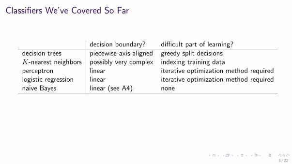
Classifiers We’ve Covered So Far
decision boundary? difficult part of learning?
decision trees piecewise-axis-aligned greedy split decisionsK-nearest neighbors possibly very complex indexing training dataperceptron linear iterative optimization method requiredlogistic regression linear iterative optimization method requirednaıve Bayes linear (see A4) none
3 / 22
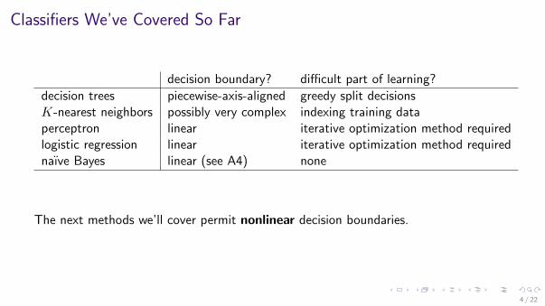
Classifiers We’ve Covered So Far
decision boundary? difficult part of learning?
decision trees piecewise-axis-aligned greedy split decisionsK-nearest neighbors possibly very complex indexing training dataperceptron linear iterative optimization method requiredlogistic regression linear iterative optimization method requirednaıve Bayes linear (see A4) none
The next methods we’ll cover permit nonlinear decision boundaries.
4 / 22
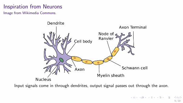
Inspiration from NeuronsImage from Wikimedia Commons.
Input signals come in through dendrites, output signal passes out through the axon.
5 / 22
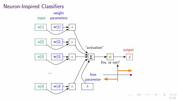
Neuron-Inspired Classifiers
x[1]
…
w[1] ×
x[2] w[2] ×
x[3] w[3] ×
x[d] w[d] ×
∑
b
!
fire, or not?ŷ
bias parameter
weight parameters
“activation” output
input
6 / 22

Neuron-Inspired Classifiers
x[1]
…
w[1] ×
x[2] w[2] ×
x[3] w[3] ×
x[d] w[d] ×
∑
b
! ŷoutput
input
f
7 / 22
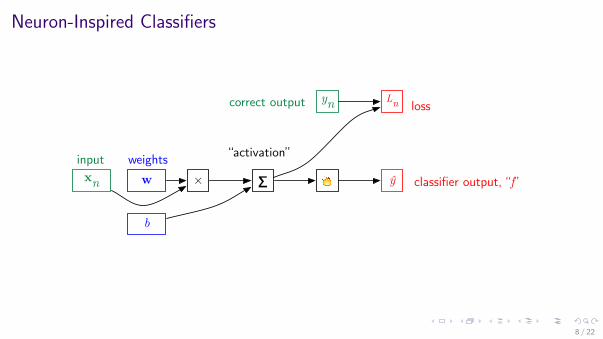
Neuron-Inspired Classifiers
xn w × ∑
b
Lnyn
! ŷweights “activation”
classifier output, “f”input
correct output loss
8 / 22
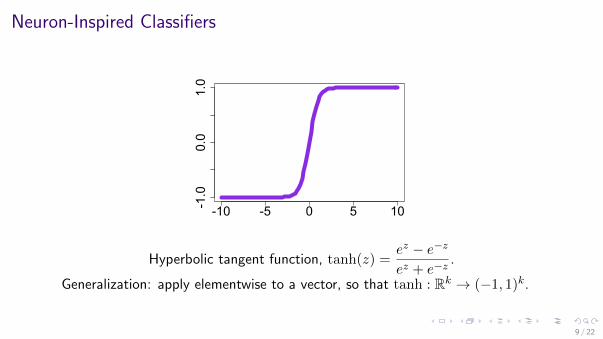
Neuron-Inspired Classifiers
-10 -5 0 5 10-1.0
0.0
1.0
Hyperbolic tangent function, tanh(z) =ez − e−z
ez + e−z.
Generalization: apply elementwise to a vector, so that tanh : Rk → (−1, 1)k.
9 / 22
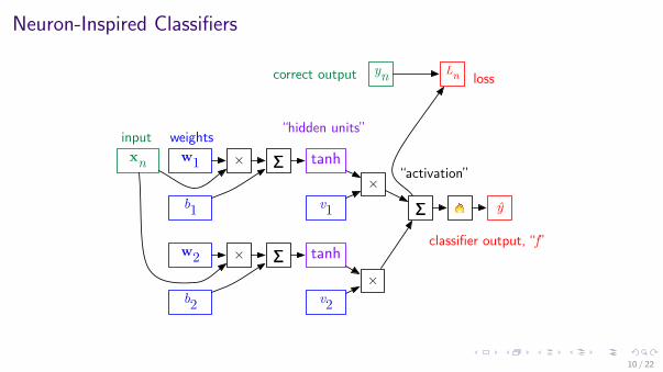
Neuron-Inspired Classifiers
xn w1 × ∑
b1
Lnyn
tanh
ŷ
weights
classifier output, “f”
input
correct output loss
w2 × ∑
b2
tanh
v1×
v2
∑
×
!
“activation”
“hidden units”
10 / 22
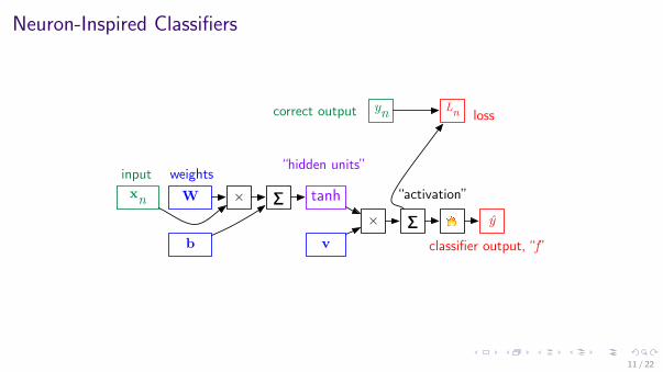
Neuron-Inspired Classifiers
xn W × ∑
b
Lnyn
tanhŷ
weights
classifier output, “f”
input
correct output loss
v× ∑ !
“activation”
“hidden units”
11 / 22
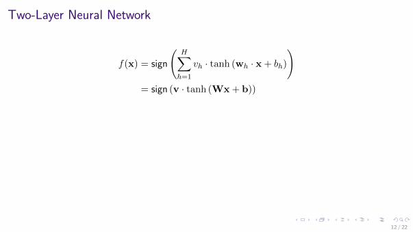
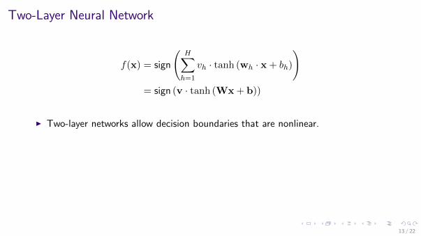
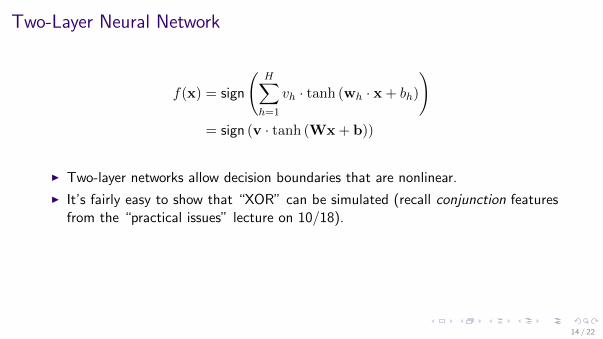
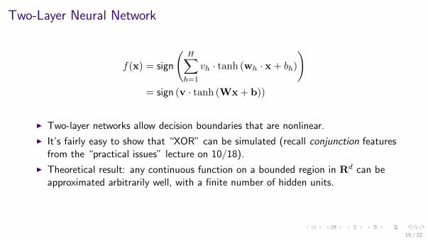
Two-Layer Neural Network
f(x) = sign
(H∑
h=1
vh · tanh (wh · x+ bh)
)= sign (v · tanh (Wx+ b))
I Two-layer networks allow decision boundaries that are nonlinear.
I It’s fairly easy to show that “XOR” can be simulated (recall conjunction featuresfrom the “practical issues” lecture on 10/18).
I Theoretical result: any continuous function on a bounded region in Rd can beapproximated arbitrarily well, with a finite number of hidden units.
I The number of hidden units affects how complicated your decision boundary canbe and how easily you will overfit.
12 / 22
Two-Layer Neural Network
f(x) = sign
(H∑
h=1
vh · tanh (wh · x+ bh)
)= sign (v · tanh (Wx+ b))
I Two-layer networks allow decision boundaries that are nonlinear.
I It’s fairly easy to show that “XOR” can be simulated (recall conjunction featuresfrom the “practical issues” lecture on 10/18).
I Theoretical result: any continuous function on a bounded region in Rd can beapproximated arbitrarily well, with a finite number of hidden units.
I The number of hidden units affects how complicated your decision boundary canbe and how easily you will overfit.
13 / 22
Two-Layer Neural Network
f(x) = sign
(H∑
h=1
vh · tanh (wh · x+ bh)
)= sign (v · tanh (Wx+ b))
I Two-layer networks allow decision boundaries that are nonlinear.
I It’s fairly easy to show that “XOR” can be simulated (recall conjunction featuresfrom the “practical issues” lecture on 10/18).
I Theoretical result: any continuous function on a bounded region in Rd can beapproximated arbitrarily well, with a finite number of hidden units.
I The number of hidden units affects how complicated your decision boundary canbe and how easily you will overfit.
14 / 22
Two-Layer Neural Network
f(x) = sign
(H∑
h=1
vh · tanh (wh · x+ bh)
)= sign (v · tanh (Wx+ b))
I Two-layer networks allow decision boundaries that are nonlinear.
I It’s fairly easy to show that “XOR” can be simulated (recall conjunction featuresfrom the “practical issues” lecture on 10/18).
I Theoretical result: any continuous function on a bounded region in Rd can beapproximated arbitrarily well, with a finite number of hidden units.
I The number of hidden units affects how complicated your decision boundary canbe and how easily you will overfit.
15 / 22

Two-Layer Neural Network
f(x) = sign
(H∑
h=1
vh · tanh (wh · x+ bh)
)= sign (v · tanh (Wx+ b))
I Two-layer networks allow decision boundaries that are nonlinear.
I It’s fairly easy to show that “XOR” can be simulated (recall conjunction featuresfrom the “practical issues” lecture on 10/18).
I Theoretical result: any continuous function on a bounded region in Rd can beapproximated arbitrarily well, with a finite number of hidden units.
I The number of hidden units affects how complicated your decision boundary canbe and how easily you will overfit.
16 / 22
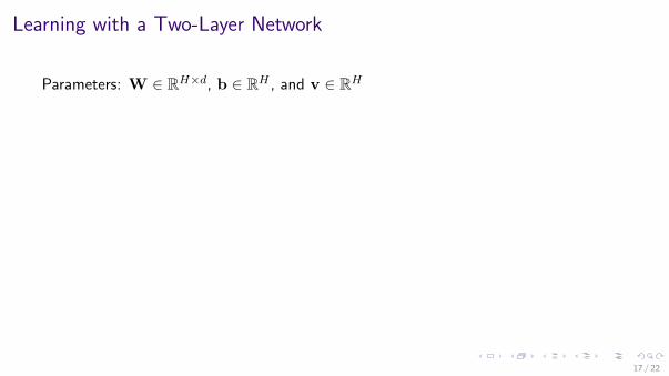
Learning with a Two-Layer Network
Parameters: W ∈ RH×d, b ∈ RH , and v ∈ RH
I If we choose a differentiable loss, then the the whole function will be differentiablewith respect to all parameters.
I Because of the squashing function, which is not convex, the overall learningproblem is not convex.
I What does (stochastic) (sub)gradient descent do with non-convex functions?
I To calculate gradients, we need to use the chain rule from calculus.
I Special name for (S)GD with chain rule invocations: backpropagation.
17 / 22
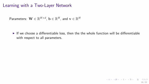
Learning with a Two-Layer Network
Parameters: W ∈ RH×d, b ∈ RH , and v ∈ RH
I If we choose a differentiable loss, then the the whole function will be differentiablewith respect to all parameters.
I Because of the squashing function, which is not convex, the overall learningproblem is not convex.
I What does (stochastic) (sub)gradient descent do with non-convex functions?
I To calculate gradients, we need to use the chain rule from calculus.
I Special name for (S)GD with chain rule invocations: backpropagation.
18 / 22
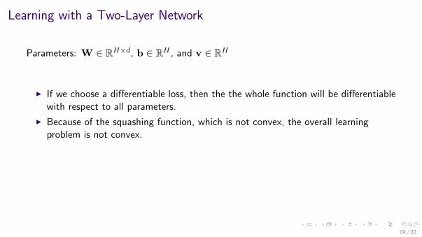
Learning with a Two-Layer Network
Parameters: W ∈ RH×d, b ∈ RH , and v ∈ RH
I If we choose a differentiable loss, then the the whole function will be differentiablewith respect to all parameters.
I Because of the squashing function, which is not convex, the overall learningproblem is not convex.
I What does (stochastic) (sub)gradient descent do with non-convex functions?
I To calculate gradients, we need to use the chain rule from calculus.
I Special name for (S)GD with chain rule invocations: backpropagation.
19 / 22
Learning with a Two-Layer Network
Parameters: W ∈ RH×d, b ∈ RH , and v ∈ RH
I If we choose a differentiable loss, then the the whole function will be differentiablewith respect to all parameters.
I Because of the squashing function, which is not convex, the overall learningproblem is not convex.
I What does (stochastic) (sub)gradient descent do with non-convex functions?
I To calculate gradients, we need to use the chain rule from calculus.
I Special name for (S)GD with chain rule invocations: backpropagation.
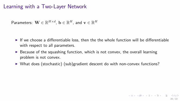
20 / 22
Learning with a Two-Layer Network
Parameters: W ∈ RH×d, b ∈ RH , and v ∈ RH
I If we choose a differentiable loss, then the the whole function will be differentiablewith respect to all parameters.
I Because of the squashing function, which is not convex, the overall learningproblem is not convex.
I What does (stochastic) (sub)gradient descent do with non-convex functions? Itfinds a local minimum.
I To calculate gradients, we need to use the chain rule from calculus.
I Special name for (S)GD with chain rule invocations: backpropagation.
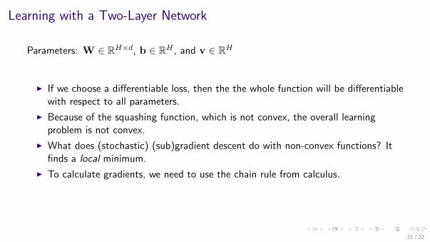
21 / 22
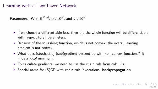
Learning with a Two-Layer Network
Parameters: W ∈ RH×d, b ∈ RH , and v ∈ RH
I If we choose a differentiable loss, then the the whole function will be differentiablewith respect to all parameters.
I Because of the squashing function, which is not convex, the overall learningproblem is not convex.
I What does (stochastic) (sub)gradient descent do with non-convex functions? Itfinds a local minimum.
I To calculate gradients, we need to use the chain rule from calculus.
I Special name for (S)GD with chain rule invocations: backpropagation.
22 / 22


