IN DEGREE PROJECT ELECTRICAL ENGINEERING, SECOND CYCLE, 30 CREDITS , STOCKHOLM SWEDEN 2016 Machine Learning for PAPR Distortion Reduction in OFDM Systems MANISH SONAL KTH ROYAL INSTITUTE OF TECHNOLOGY SCHOOL OF ELECTRICAL ENGINEERING
Transcript
IN DEGREE PROJECT ELECTRICAL ENGINEERING,SECOND CYCLE, 30 CREDITS
, STOCKHOLM SWEDEN 2016
Machine Learning for PAPR Distortion Reduction in OFDM Systems
MANISH SONAL
KTH ROYAL INSTITUTE OF TECHNOLOGYSCHOOL OF ELECTRICAL ENGINEERING
iii
Abstract
The purpose of the project is to investigate the possibility of using modernmachine learning to model nonlinear analog devices like the Power Ampli-fier (PA), and study the feasibility of using such models in wireless systemsdesign. Orthogonal frequency division multiplexing (OFDM) is one of themost prominent modulation technique used in several standards like 802.11a,802.11n, 802.11ac and more. Telecommunication systems like LTE, LTE/Aand WiMAX are also based on OFDM. Nevertheless, OFDM system showshigh peak to average power (PAPR) in time domain because it comprisesof many subcarriers added via inverse fast Fourier transform(IFFT). HighPAPR results in an increased symbol error rate, while degrading the effi-ciency of the PA. Digital predistortion (DPD) still suffers from high symbolerror rate (SER) and reduced PA efficiency, when there is an increase in peakback off(PBO). A receiver based nonlinearity distortion reduction approachcan be justified by the fact that base stations have high computation power.A iterative-decision-feedback mitigation technique can be implemented as areceiver side compensation assuming memoryless PA nonlinearities. For suc-cessful distortion reduction the iterative-decision based technique required theknowledge of the transmitter PA. The author proposes to identify the nonlin-ear PA model using machine learning techniques like nonlinear regression anddeep learning. The results show promising improvement in SER reductionwith small PA model learning time.
Index Terms- OFDM, machine learning, PAPR, neural networks
iv
Sammanfattning
Syftet med detta projekt är att undersöka möjligheterna att använda modernmaskininlärning för att beskriva ickelinjära analoga enheter såsom effektförstär-kare och att studera hur användbart det är att använda sådana modeller föratt designa trådlösa kommunikationssystem. OFDM (ortogonal frekvensmulti-plex) är en av de vanligast förekommande modulationsteknikerna, som användsi standarder såsom 802.11a, 802.11n, 802.11ac and andra. Telekommunikations-system som LTE, LTE/A och WiMAX baseras också på OFDM. Dock resulterarOFDM i hög toppeffekt i förhållande till medeleffekten (hög PAPR) i tidsdomä-nen, eftersom signalen består av många delkanaler som summeras mha inversdiskret fouriertransform (IFFT). En hög PAPR resulterar i ökad symbolfelshaltoch försämrar effektiviteten hos effektförstärkaren. Digital predistortion (DPD)kan förbättra situationen men ger fortfarande hög symbolfelshalt och försämradförstärkareffektivitet, när man drar ned sändeffekten för undvika kvarvarandeickelineariteter. Att minska förvrängningen från ickelineariteterna vid mottaga-ren kan motiveras i system där basstationerna har hög beräkningsförmåga. Enmetod för att reducera förvrängningarna kan implementeras på mottagarsidan,baserad på iterativ beslutsåterkoppling, under antagandet om att sändarens ef-fektförstärkare har en minneslös ickelinearitet. För att störningsreduceringenska fungera väl, krävs god kunskap om sändarens effektförstärkare. Författarenföreslår att identifiera en ickelinjär modell för förstärkaren mha maskininlär-ningstekniker, såsom ickelinjär regression och djup inlärning. Resultaten visarlovande förbättringar av symbolfelshalten med en låg inlärningstid för förstär-karmodellen.
v
Acknowledgment
I would like to express my deepest gratitude to Prof. Dr. Mats Bengtsson, for hisexcellent guidance and caring. There were times when I was lost in the work andone small suggestion from him helped me get the right research direction. I feelprivileged to have worked with him and I am grateful for his support.
I would like to extend my gratitude to my friends at the KTH Electrical schoolMaster thesis room, It was fun discussing the project problem with them over thefika breaks. I dedicate this thesis to my parents, my brother Amit, my sisters Sweta,Manisha and Neha, and my girlfriend Priya for moral support they provided meduring my studies. I would also like to thank my friend Mantosh for reviewing thecontent and helping me improve the literature readability.
4.1 Idea PA Solid State PA model used at Transmitter . . . . . . . . . . . . 324.2 PA fit using Smoothing spline . . . . . . . . . . . . . . . . . . . . . . . . 344.3 PA fit Polynomial fit . . . . . . . . . . . . . . . . . . . . . . . . . . . . . 364.4 Neural Network training and performance, 25800X6 data set . . . . . . 394.5 Neural Network PA estimated model, 25800X6 data set . . . . . . . . . 394.6 Neural Network training and performance, 77400X6 data set . . . . . . 404.7 Neural Network PA estimated model, 77400X6 data set . . . . . . . . . 404.8 Neural Network training and performance, 172000X6 data set . . . . . . 414.9 Neural Network PA estimated model, 172000X6 data set . . . . . . . . . 424.10 Symbol Error Rate vs SNR for IFB, distortion due to PA nonlinearity,
PA Saturation 7.0dB . . . . . . . . . . . . . . . . . . . . . . . . . . . . . 434.11 QAM scatter plot without IFB, nonlinear distortion due to PA . . . . . 444.12 QAM scatter plot with IFB, nonlinear distortion due to PA . . . . . . . 454.13 Symbol Error Rate vs SNR for IFB, distortion due to clipping plus PA
4.15 QAM scatter plot with IFB, nonlinear distortion due to clipping plus PA 474.16 Symbol Error Rate vs SNR for IFB, distortion due to PA nonlinearity,
OFDM can be thought as a nexus of modulation and multiplexing in which we sharethe bandwidth among individual modulated data sources. Normally the modula-tion techniques are single carrier but OFDM employs several carriers, within theallocated bandwidth. Each of the carriers then employs one or several of the avail-able digital methods like BPSK, QPSK, QAM etc. Filter based implementationof multicarrier modulation existed in literature in 1960’ [1]. Implementation ofOFDM with Fourier transform gave a breakthrough in multicarrier modulation(MCM) techniques [2], and increased its implementation feasibility with less com-plex electronics. Today OFDM is used in many wireless standards like 802.11a,802.11n, 802.11ac along with latest telecommunication systems like LTE, LTE/Aand WiMAX.
1.1 What is OFDM?
OFDM is a multicarrier modulation scheme in which the total bandwidth is dividedinto smaller orthogonal subcarriers. Each subcarrier is then modulated with adifferent digital data stream. When information symbols are modulated with manycarriers, then the sidebands normally spread out inside neighbouring subcarriers.The receiver in this case will be able to demodulate only when there is a considerableseparation between the carriers. Have a look at Fig. 1.1, for receiving informationover multiple carriers. There has to be a separation between the different carrierfrequencies else intercarrier interference(ICI) will occur. OFDM is different fromtraditional modulation in this sense, even though all the sidebands overlap, still,the information can be received. The reason for this is the fact that in OFDM thesubcarriers are orthogonal to each other. This is achieved by dividing the availablebandwidth into multiple carriers, with equal spacing, where the spacing is equal tothe reciprocal of the symbol period.
To get a clear understanding of OFDM, it is good to revisit an OFDM receiver.The received signal is integrated over the symbol period to demodulate the data
1
2 CHAPTER 1. INTRODUCTION
Figure 1.1: Simplified model of multiple signal filtering required in traditional re-ceiver
from that carrier. In simpler words, the integration works on fact that, if we aredemodulating for the lth subcarrier, then all subcarriers except the lth subcarrierare orthogonal to the lth subcarrier. Thus there is no interference contribution.
Normalized frequency
-3 -2 -1 0 1 2 3
Am
plit
ud
e
-0.5
0
0.5
1
1.5Carrier 1
sampling, carrier 1
Carrier 2
Sampling, carrier 2
Carrier 3
Sampling, Carrier 3
Normalized frequency
-3 -2 -1 0 1 2 3
Am
plit
ud
e
-0.5
0
0.5
1
1.5
Sum of all subcarriers
sampling point
Only carrier 1 is non zero at this frequency
Figure 1.2: Frequency domain visualization of OFDM
1.1. WHAT IS OFDM? 3
Have a look a Fig. 1.2, there are 3 subcarriers modulated with some data, inthe first figure you can easily see that all the subcarriers are independent of eachother. The sampling point where carrier-1 is nonzero, all the other subcarriers arezero, same is valid for carrier-2 and carrier-3. The second subfigure is the sum ofall subcarriers, if we sample exactly at the original sampling point, the informationis preserved. Now one can have a very genuine question, how many subcarriers
-8 -6 -4 -2 0 2 4 6 8
Normalized frequency
-0.5
0
0.5
1
1.5
Am
plit
ude
OFDM subcarriers in frequency domain
-8 -6 -4 -2 0 2 4 6 8
Normalized frequency
-0.5
0
0.5
1
1.5
Am
plit
ude
Sum of all subcarriers in frequency domain
Sum(all subcarriers)
Sampling pointIncorrect sampled
value due to
frequncy drift
Figure 1.3: Frequency domain visualization of OFDM, with frequency drift
can we split the available bandwidth into. Example if we have 10MHz as availablebandwidth and we split it into 1000 subcariers of 10KHz each, with each subcarriercarrying 10 bits of information then we can transmit 10Kbits of information everysecond, but if we split 10MHz into 100 subcarriers with each carrying 10 bits ofinformation, data rate would be 1Kbits per second, which is very small. Thus wewould definitely like to divide the available bandwidth into as many numbers ofsubcarriers as possible. There is a limit to it, we can not place the subcarriers veryclose to each other as there can be high ICI and ISI. As a kind optimal solution,
4 CHAPTER 1. INTRODUCTION
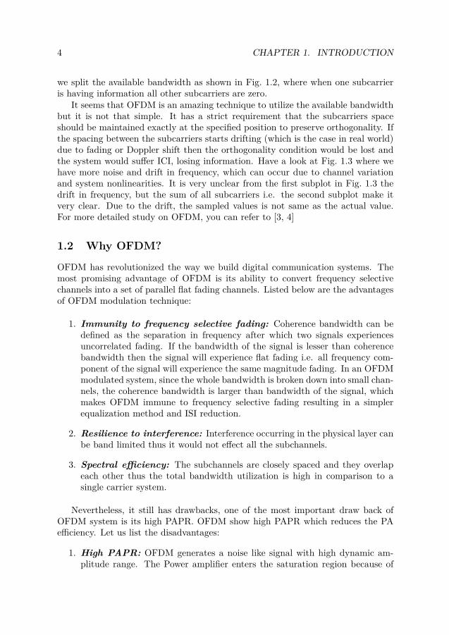
we split the available bandwidth as shown in Fig. 1.2, where when one subcarrieris having information all other subcarriers are zero.
It seems that OFDM is an amazing technique to utilize the available bandwidthbut it is not that simple. It has a strict requirement that the subcarriers spaceshould be maintained exactly at the specified position to preserve orthogonality. Ifthe spacing between the subcarriers starts drifting (which is the case in real world)due to fading or Doppler shift then the orthogonality condition would be lost andthe system would suffer ICI, losing information. Have a look at Fig. 1.3 where wehave more noise and drift in frequency, which can occur due to channel variationand system nonlinearities. It is very unclear from the first subplot in Fig. 1.3 thedrift in frequency, but the sum of all subcarriers i.e. the second subplot make itvery clear. Due to the drift, the sampled values is not same as the actual value.For more detailed study on OFDM, you can refer to [3, 4]
1.2 Why OFDM?
OFDM has revolutionized the way we build digital communication systems. Themost promising advantage of OFDM is its ability to convert frequency selectivechannels into a set of parallel flat fading channels. Listed below are the advantagesof OFDM modulation technique:
1. Immunity to frequency selective fading: Coherence bandwidth can bedefined as the separation in frequency after which two signals experiencesuncorrelated fading. If the bandwidth of the signal is lesser than coherencebandwidth then the signal will experience flat fading i.e. all frequency com-ponent of the signal will experience the same magnitude fading. In an OFDMmodulated system, since the whole bandwidth is broken down into small chan-nels, the coherence bandwidth is larger than bandwidth of the signal, whichmakes OFDM immune to frequency selective fading resulting in a simplerequalization method and ISI reduction.
2. Resilience to interference: Interference occurring in the physical layer canbe band limited thus it would not effect all the subchannels.
3. Spectral efficiency: The subchannels are closely spaced and they overlapeach other thus the total bandwidth utilization is high in comparison to asingle carrier system.
Nevertheless, it still has drawbacks, one of the most important draw back ofOFDM system is its high PAPR. OFDM show high PAPR which reduces the PAefficiency. Let us list the disadvantages:
1. High PAPR: OFDM generates a noise like signal with high dynamic am-plitude range. The Power amplifier enters the saturation region because of
1.3. PROBLEM FORMULATION - PURPOSE AND GOALS 5
the high peak powers in an OFDM system. This reduces the system perfor-mance considerably, as the PA operates in nonlinear region there is significantinformation loss.
2. Highly sensitive to frequency offset: OFDM based communication sys-tems are very much sensitive to carrier offset and frequency drift. We had acloser look at this in the last section 1.1
1.3 Problem formulation - Purpose and Goals
Figure 1.4: Practical Power Amplifier
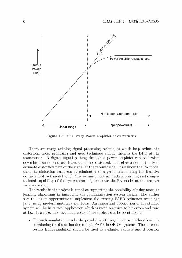
Power amplifiers in transceivers consists of three stage amplification, the PreDriver and Driver stage provide the actual amplification in power with gains greaterthan one while, the final stage is designed to match impedance with antenna andtransfer the amplified signal, refer Fig. 1.4. Ideally the final stage PA characteristicsshould be linear with unit gain, which is practically not possible. This makesDesign of final stage amplifier costly in terms of complexity moreover it is the mostpower hungry part of PA. A non ideal behavior of final stage leads to considerablesignal distortion and loss in battery life. The Linear operation of final stage poweramplifiers used in communication systems is limited to a specific dynamic range.The transistors get saturated after a certain input voltage and thus the amplificationbeyond the saturation region give rise to information loss. When the peak power isvery high in an OFDM system it gets amplified from the nonlinear region of the PAresulting in information loss. Consider Fig. 1.5, the input-output characteristics ofthe final stage PA becomes nonlinear after a certain point, because the transistorshave a saturation limit. Thus any input power beyond this linear region will givea constant amplification, which will distort the signal resulting in information loss.Hence, high PAPR in OFDM system results in power amplifier saturation, leadingto intercarrier interference and increase in SER. The research question consideredin this paper deals with reducing the final stage PA distortion effect in OFDMsystem due to its high PAPR using Machine learning algorithms. We will do adetailed analysis of PAPR in chapter 3.
6 CHAPTER 1. INTRODUCTION
Figure 1.5: Final stage Power amplifier characteristics
There are many existing signal processing techniques which help reduce thedistortion, most promising and used technique among them is the DPD at thetransmitter. A digital signal passing through a power amplifier can be brokendown into components as distorted and not distorted. This gives an opportunity toestimate distortion part of the signal at the receiver side. If we know the PA modelthen the distortion term can be eliminated to a great extent using the iterativedecision feedback model [5, 6]. The advancement in machine learning and compu-tational capability of the system can help estimate the PA model at the receiververy accurately.
The results in the project is aimed at supporting the possibility of using machinelearning algorithms in improving the communication system design. The authorsees this as an opportunity to implement the existing PAPR reduction technique[5, 6] using modern mathematical tools. An Important application of the studiedsystem will be in critical application which is more sensitive to bit errors and runsat low data rate. The two main goals of the project can be identified as
• Through simulation, study the possibility of using modern machine learningin reducing the distortion due to high PAPR in OFDM systems. The outcomeresults from simulation should be used to evaluate, validate and if possible
1.4. PROJECT METHODOLOGY 7
improve the existing theory. The outcome should also provide related ideasas a part of future research work.
• As a part of Masters program, the project accounts for 30 E.C.T.S with aminimum workload of 20 weeks.
1.4 Project methodology
The methodology followed in this project is simple and systematic for a scientificproject. As a preliminary step one has to think about background study, thiswas achieved by reading relevant journal papers on OFDM and PAPR nonlinearitymitigation techniques. Details about modern machine learning algorithm and itsimplementation were acquired from online course available at Coursera and Udacity.However, several tutorial papers and books were used to acquired the fundamentalknowledge of OFDM and digital communication in general. Some of the papers [5, 6]have made a remarkable contribution to PAPR nonlinearity mitigation techniquesand forms the basis of this project.
The execution of the project was a major part of understanding and knowledgeacquisition. Simulations in MATLAB was used as the way to evaluate the per-formance of decision feedback nonlinearity mitigation, when PA model is learnedusing different machine learning technique. Machine learning model learning timedepends on the capability of the machine. In this project, all the machine learn-ing model simulation were done in MATLAB on a windows system with Intel i-7CPU. The results and model design were discussed with the supervisor from timeto time, this made it sure that the project is moving in right direction and resultare accurate.
Meanwhile, over the entire project execution, the acquired knowledge and simu-lation results were documented. In order to make the results more understandablefor the readers, relevant theory and system model was well written and system-atically presented in the report (this report). At the end of the project, a smallpresentation was conducted to present the theoretical understanding and experi-mental results.
1.5 Outline
The rest of this document is organized as follows:
• In chapter 2, the required background is presented. It provides the technicaltheory in relation to the project objective moreover this chapter describes thedistortion removal algorithm in detail.
• In chapter 3, we present the system model and key parameters that are in-vestigated in this project.
• In chapter 4, we present the simulation results of the investigated schemes.
8 CHAPTER 1. INTRODUCTION
• In chapter 5, we introduce suggested future works related to the project andwe conclude the work in this chapter.
Chapter 2
Theory
There has been constant research going on to resolve the distortion problem inOFDM system due to high PAPR. In this chapter, we will go through the types ofPA nonlinearities later we discuss some of the widely used nonlinearity distortionreduction techniques in the industry. One of the studied model forms the basis ofour distortion compensation algorithm.
2.1 Types of nonlinearity
Before discussing the nonlinearity mitigation technique it is important to under-stand the types of nonlinearity generated by the PA. In this section, we will gothrough the memory and memoryless nonlinearity although for the implementationpurpose the paper considers the memoryless PA scenario.
2.1.1 Power amplifier memoryless nonlinearityMany nonlinear devices like the limiter and power amplifier can be precisely mod-eled as linear devices. If fpa(.) is the nonlinear response from the PA, the outputin discrete term can be written as
xfpa [n] = fpa(x[n]) (2.1)
From Bussgang’s theorem, we know that in a memoryless system the crosscorrelation between the input and output has the same shape as the autocorrelationbetween the inputs [7] [8, chapter 6]. In other words
< x(t+ τ)xfpa(t) > = α. < x(t+ τ)x(t) > (2.2)
from Eq. 2.2 we can derive that
xfpa(t) = α.x(t) + y(t) (2.3)
9
10 CHAPTER 2. THEORY
where y(t) will be uncorrelated with x(t) i.e. the PA model can be represented asa cascade of linear and nonliner function.
< x(t+ τ)y(t) > = 0 (2.4)
Following derivations in [7] , we can write that complex envelope of the outputsignal from a memoryless high power amplifier as [6]
fpa(x) = A(ρ).e(φ+P [ρ]) (2.5)
considering input as polar function represented as
x = ρ.ejφ (2.6)
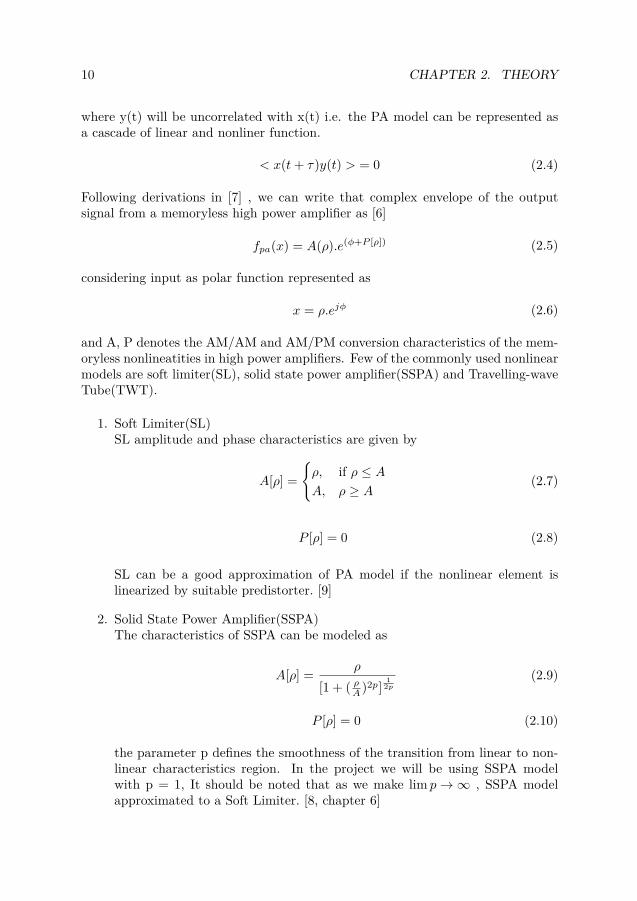
and A, P denotes the AM/AM and AM/PM conversion characteristics of the mem-oryless nonlineatities in high power amplifiers. Few of the commonly used nonlinearmodels are soft limiter(SL), solid state power amplifier(SSPA) and Travelling-waveTube(TWT).
1. Soft Limiter(SL)SL amplitude and phase characteristics are given by
A[ρ] ={ρ, if ρ ≤ AA, ρ ≥ A
(2.7)
P [ρ] = 0 (2.8)
SL can be a good approximation of PA model if the nonlinear element islinearized by suitable predistorter. [9]
2. Solid State Power Amplifier(SSPA)The characteristics of SSPA can be modeled as
A[ρ] = ρ
[1 + ( ρA )2p]1
2p(2.9)
P [ρ] = 0 (2.10)
the parameter p defines the smoothness of the transition from linear to non-linear characteristics region. In the project we will be using SSPA modelwith p = 1, It should be noted that as we make lim p→∞ , SSPA modelapproximated to a Soft Limiter. [8, chapter 6]
2.2. DIGITAL PREDISTORTION TECHNIQUE(DPD) 11
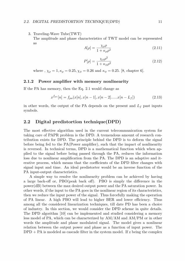
3. Traveling-Wave Tube(TWT)The amplitude and phase characteristics of TWT model can be representedas
A[ρ] = χρρ
1 + κρρ2 (2.11)
P [ρ] = χφρ2
1 + κφρ2 (2.12)
where , χρ = 1, κρ = 0.25, χφ = 0.26 and κφ = 0.25. [8, chapter 6].
2.1.2 Power amplifier with memory nonlinearityIf the PA has memory, then the Eq. 2.1 would change as
in other words, the output of the PA depends on the present and Lf past inputssymbols.
2.2 Digital predistortion technique(DPD)
The most effective algorithm used in the current telecommunication system fortaking care of PAPR problem is the DPD. A tremendous amount of research con-tribution exists for DPD. The principle behind the DPD is to deform the signalbefore being fed to the PA(Power amplifier), such that the impact of nonlinearityis reversed. In technical terms, DPD is a mathematical function which when ap-plied to the signal before being passed through the PA, reduces the informationloss due to nonlinear amplification from the PA. The DPD is an adaptive and it-erative process, which means that the coefficients of the DPD filter changes withsignal input and time. An ideal predistorter would be an inverse function of thePA input-output characteristics.
A simple way to resolve the nonlinearity problem can be achieved by havinga large back-off or, PBO(peak back off). PBO is simply the difference in thepower(dB) between the max desired output power and the PA saturation power. Inother words, if the input to the PA goes in the nonlinear region of its characteristics,then we reduce the input power of the signal. Thus forcefully making the operationof PA linear. A high PBO will lead to higher BER and lower efficiency. Thusamong all the considered linearization techniques, till date PD has been a choiceof industry. In this section, we would consider the DPD scheme in quite details.The DPD algorithm [10] can be implemented and studied considering a memoryless model of PA, which can be characterized by AM/AM and AM/PM or in otherwords the amplitude and phase modulated signal. The model gives a nonlinearrelation between the output power and phase as a function of input power. TheDPD + PA is modeled as cascade filter in the system model. If z being the complex
12 CHAPTER 2. THEORY
envelope at the PA input, following Eq. 2.5 the output at the PA can be modeledas
A(Z) = AM(|z|2)ej(arg(z)+PM(|z|2)) (2.14)
where AM(|z|2) and PM(|z|2) are the AM/AM and AM/PM component charac-teristics. The DPD is designed to follow up a rule such that the difference betweenthe output of the PA and the original signal is minimum. In [11], the authors haveconsidered a more practical scenario i.e. a frequency-selective fading channel andevaluated the performance of PD techniques in an OFDM modulated system. Theauthors have considered a traveling wave tube (TWT) model of a PA [12]. Theamplitude and phase characteristics of a TWT model is approximated as
M(ρ) = 2ρ1 + ρ2 (2.15)
Φ(ρ) = Φ02ρ2
1 + ρ2 (2.16)
where Φ0 = π6 and ρ denote the input signal amplitude. Further, the author
considered the timevariant multipath channel is modeled as the impulse responseof the following form.
h(t) =Np−1∑i=0
diejθiδ(t− τi) (2.17)
where Np is the number of multipath channels, di , θi and τi gives amplitude ,phase rotation and propagation delays associated with the ith path. In [11] , theauthor has compared the performance of MMSE scheme with the Amplitude andphase pre-distortion. The results are quite positive for Amplitude and phase PDtechnique. In a general case, the output is y(t) of the DPD is modeled as theproduct of input x(t) (eg., A QAM modulated symbol after IFFT operation) anda nonlinear memoryless device consisting of two parallel branches, upper branch isthe amplitude branch which helps cancel nonlinear AM/AM response of HPA whilethe lower is the phase branch which helps cancel the AM/PM nonlinearity.
2.3 Neural network based PAPR mitigation
In [13] the author has proposed a Neural Network based approach to reduce the non-linearity. The Author directly estimates the signal constellation based on ACE(Activeconstellation extension) trained Neural Network. The author names his approachas TFNN ( Time Frequency Neural network) since ACE takes into account thetime and frequency domain distortion simultaneous. In ACE the signal peaks arereduced by clipping exceeding magnitudes in the time domain moreover in the fre-quency domain the movement of constellation point is restricted to only acceptablevalues. The model is trained separately on the complex and real part of the sym-bols as two neural networks set asModelTNNReal andModelTNNImaginary. the transmitter
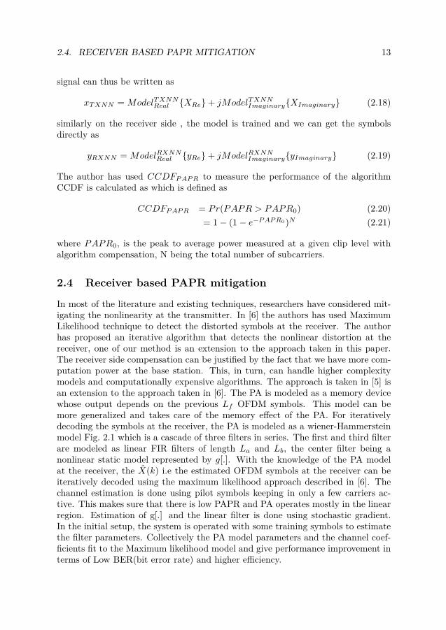
where PAPR0, is the peak to average power measured at a given clip level withalgorithm compensation, N being the total number of subcarriers.
2.4 Receiver based PAPR mitigation
In most of the literature and existing techniques, researchers have considered mit-igating the nonlinearity at the transmitter. In [6] the authors has used MaximumLikelihood technique to detect the distorted symbols at the receiver. The authorhas proposed an iterative algorithm that detects the nonlinear distortion at thereceiver, one of our method is an extension to the approach taken in this paper.The receiver side compensation can be justified by the fact that we have more com-putation power at the base station. This, in turn, can handle higher complexitymodels and computationally expensive algorithms. The approach is taken in [5] isan extension to the approach taken in [6]. The PA is modeled as a memory devicewhose output depends on the previous Lf OFDM symbols. This model can bemore generalized and takes care of the memory effect of the PA. For iterativelydecoding the symbols at the receiver, the PA is modeled as a wiener-Hammersteinmodel Fig. 2.1 which is a cascade of three filters in series. The first and third filterare modeled as linear FIR filters of length La and Lb, the center filter being anonlinear static model represented by g[.]. With the knowledge of the PA modelat the receiver, the X(k) i.e the estimated OFDM symbols at the receiver can beiteratively decoded using the maximum likelihood approach described in [6]. Thechannel estimation is done using pilot symbols keeping in only a few carriers ac-tive. This makes sure that there is low PAPR and PA operates mostly in the linearregion. Estimation of g[.] and the linear filter is done using stochastic gradient.In the initial setup, the system is operated with some training symbols to estimatethe filter parameters. Collectively the PA model parameters and the channel coef-ficients fit to the Maximum likelihood model and give performance improvement interms of Low BER(bit error rate) and higher efficiency.
14 CHAPTER 2. THEORY
Figure 2.1: Power amplifier model as a cascade of linear and nonlinear filters
In this project, we have used the distortion removal approach take in [6], wename this method as Iterative feedback(IFB). We will use IFB for mitigating PAPRnonliterary. The next section describes and presents a detailed analysis of thealgorithm.
2.4.1 Iterative feedback(IFB)In this approach, we would try to remove the distortion with an iterative feedbacksystem. We assume that the nonlinearity due to PA happens at the transmitterand trying to mitigate at the receiver. If the nonlinearity is present in discretetime domain then this analysis gives accurate result however if the nonlinearity ispresent in continuous time domain then this analysis gives approximate results, butit can be accurate with oversampling taking care of the spectral regrowth.
The output of the memoryless nonlinearity can be modeled as [6, 7] [8, chapter 6]
xfpanL
= fpa(x nL
)
= α.x nL
+ dn(X) (2.22)
where xn is the input to PA, fpa id the power amplifier learned model and Lbeing the oversampling. As explained in [7] the output can be expressed as a linearcombination of actual amplified input to PA and a distortion term. The constantterm α is selected such that the MSE E[|fpa(x n
L) − α.x n
L|2] is minimized. The
term dn(X)
thus contains the distortion energy and is uncorrelated with x xL. It
is proved that for SL and SSPA nonlinearity , α → 1 for clip level > 7.3dB. [14].If the channel intersymbol interference is shorter than cyclic prefix, the distortionis limited to a single multicarrier symbol. Now we can see that distortion is adeterministic function of x n
L, so d(X)
n . thus the QAM vector of pth symbol XpL that
will contain the nonlineatiy distortion can be computer FFT from Eq. 2.22 overthe whole interval including oversampling discrete intervals. Mathematically
FFT (xfpa,pnL
) = Xfpa,pL = Xm
L +D(fpa,Xp)L (2.23)
2.4. RECEIVER BASED PAPR MITIGATION 15
Figure 2.2: Iterative feedback model
if k being the time index, we can expand Eq. 2.23
FFT (xfpa,pnL
) =
Xmk +D
(fpa,Xp)L,k , k = 0, ...., N2 − 1
D(fpa,Xp)L,k , k = N
2 , ...., NL−N2 − 1
Xmk−N(L−1) +D
(fpa,Xp)L,k , k = NL− N
2 − 1, ...., NL− 1.(2.24)
D(fpa,Xp)L,k , k = N
2 , ...., NL −N2 − 1 is the out of band distortion and we will use
clipping windowing to minimize this. For all further explanation and receiver de-sign, we will drop the symbol index p and oversampling L to maintain simplicityin equation representations. Moreover, we assume that out of band distortion isremoved at the receiver before the distortion mitigation algorithm is applied. If Hk
is the FFT of channel impulse response h[n], then we can get the received symbolsas
Yfpak = Hk(Xk +D
(fpa,X)k ) +Noisek (2.25)
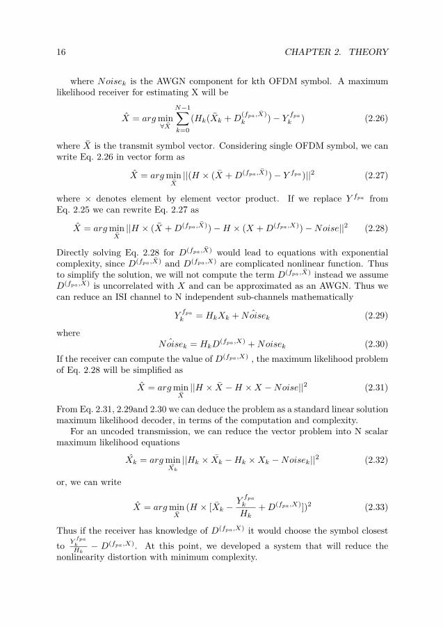
16 CHAPTER 2. THEORY
where Noisek is the AWGN component for kth OFDM symbol. A maximumlikelihood receiver for estimating X will be
X = argmin∀X
N−1∑k=0
(Hk(Xk +D(fpa,X)k )− Y fpak ) (2.26)
where X is the transmit symbol vector. Considering single OFDM symbol, we canwrite Eq. 2.26 in vector form as
X = argminX||(H × (X +D(fpa,X))− Y fpa)||2 (2.27)
where × denotes element by element vector product. If we replace Y fpa fromEq. 2.25 we can rewrite Eq. 2.27 as
X = argminX||H × (X +D(fpa,X))−H × (X +D(fpa,X))−Noise||2 (2.28)
Directly solving Eq. 2.28 for D(fpa,X) would lead to equations with exponentialcomplexity, since D(fpa,X) and D(fpa,X) are complicated nonlinear function. Thusto simplify the solution, we will not compute the term D(fpa,X) instead we assumeD(fpa,X) is uncorrelated with X and can be approximated as an AWGN. Thus wecan reduce an ISI channel to N independent sub-channels mathematically
Yfpak = HkXk + ˆNoisek (2.29)
whereˆNoisek = HkD
(fpa,X) +Noisek (2.30)If the receiver can compute the value of D(fpa,X) , the maximum likelihood problemof Eq. 2.28 will be simplified as
X = argminX||H × X −H ×X −Noise||2 (2.31)
From Eq. 2.31, 2.29and 2.30 we can deduce the problem as a standard linear solutionmaximum likelihood decoder, in terms of the computation and complexity.
For an uncoded transmission, we can reduce the vector problem into N scalarmaximum likelihood equations
Xk = argminXk
||Hk × Xk −Hk ×Xk −Noisek||2 (2.32)
or, we can write
X = argminX
(H × [Xk −Yfpak
Hk+D(fpa,X)])2 (2.33)
Thus if the receiver has knowledge of D(fpa,X) it would choose the symbol closestto Y
fpak
Hk− D(fpa,X). At this point, we developed a system that will reduce the
nonlinearity distortion with minimum complexity.
2.4. RECEIVER BASED PAPR MITIGATION 17
2.4.2 Implementation of IFB
How to realize the system in practice, there can be multiple ways to estimateD(fpa,X)
1. Send some extra information along with the data
2. Use feedback to iteratively estimate D(fpa,X)
Algorithm 1 : IFBRequire: [1, ..., Xrx
m ]: Received OFDm symbol blocksEnsure: H: Channel impulse response know at the receiverEnsure: fpa: Nonlinear model of the PA , estimated at the receiver using Machine
Learning1: procedure Distortion reduction algorithm( [1, ..., xn], H , fpa)2:3: for i do number of OFDM symbols4:5: Xn ← removed cyclic prefix from Xrx
m
6:7: for j do number of iterative feedback8:9: Xq = ((1/sqrt(N) ∗ FFT ([1, ....., Xn])) ./H −D(fpa,Xn−1)) . Xq the
option 1, will decrease the total data rate of the system , like the tone injec-tion(TI) [15]. As presented in section 2.4.1 Option 2, is a more intelligent wayto solve the problem. If the receiver knows the nonlinear PA function fpa(.) , itcan iteratively approximate the distortion term from the received vector Y fpa andestimate the QAM vector. Assuming that the channel information and the PAnonlinear model(estimated using Machine learning algorithm) is perfectly knownat the receiver, the algorithm can be implemented in few basic steps as show inAlgorithm 1
Chapter 3
System Model
3.1 PAPR
Let us understand how the peak power increases in an OFDM modulated systemsand how it affects our communication systems, reducing BER and degrading perfor-mance. This will help us better understand the problem considered in this project.In the following discussion we use lower case x from time domain values, and uppercase X for frequency domain values moreover x∗ denotes the complex conjugate ofx. Vectors are denoted as boldface or sequence x[n], e.g x[n] = [x0, ....xN−1]. Theindex n stands for time and k for frequency.
3.1.1 Analysis
Figure 3.1: IFFT of Information symbols
In order to understand the PAPR problem we need to look into a more detailedanalysis of an OFDMmodulated system. Consider the QAM symbols [X(0), .....X(N−1)] modulated over subcarriers 0..n. Each of the QAM having maximum amplitude
19
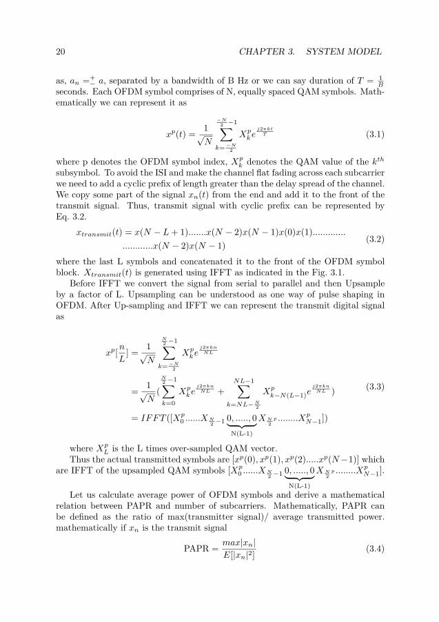
20 CHAPTER 3. SYSTEM MODEL
as, an =+− a, separated by a bandwidth of B Hz or we can say duration of T = 1
Bseconds. Each OFDM symbol comprises of N, equally spaced QAM symbols. Math-ematically we can represent it as
xp(t) = 1√N
−N2 −1∑
k= −N2
Xpke
j2πktT (3.1)
where p denotes the OFDM symbol index, Xpk denotes the QAM value of the kth
subsymbol. To avoid the ISI and make the channel flat fading across each subcarrierwe need to add a cyclic prefix of length greater than the delay spread of the channel.We copy some part of the signal xn(t) from the end and add it to the front of thetransmit signal. Thus, transmit signal with cyclic prefix can be represented byEq. 3.2.
where the last L symbols and concatenated it to the front of the OFDM symbolblock. Xtransmit(t) is generated using IFFT as indicated in the Fig. 3.1.
Before IFFT we convert the signal from serial to parallel and then Upsampleby a factor of L. Upsampling can be understood as one way of pulse shaping inOFDM. After Up-sampling and IFFT we can represent the transmit digital signalas
xp[nL
] = 1√N
N2 −1∑
k= −N2
Xpke
j2πknNL
= 1√N
(N2 −1∑k=0
Xpke
j2πknNL +
NL−1∑k=NL−N2
Xpk−N(L−1)e
j2πknNL )
= IFFT ([Xp0 ......XN
2 −1 0, ....., 0︸ ︷︷ ︸N(L-1)
XN2p ........Xp
N−1])
(3.3)
where XpL is the L times over-sampled QAM vector.
Thus the actual transmitted symbols are [xp(0), xp(1), xp(2).....xp(N−1)] whichare IFFT of the upsampled QAM symbols [Xp
0 ......XN2 −1 0, ....., 0︸ ︷︷ ︸
N(L-1)
XN2p ........Xp
N−1].
Let us calculate average power of OFDM symbols and derive a mathematicalrelation between PAPR and number of subcarriers. Mathematically, PAPR canbe defined as the ratio of max(transmitter signal)/ average transmitted power.mathematically if xn is the transmit signal
PAPR = max|xn|E[|xn|2] (3.4)
3.1. PAPR 21
where E[|xn|2] is the average signal power.
Average signal power = E[x(n).x∗(n)]
= 1N2 .E[
N2 −1∑i= −N
2
an. expj2πkiN
N2 −1∑i= −N
2
a∗n. exp−j2πkiN ]
= 1N2E[an.a∗n
N2 −1∑i= −N
2
N2 −1∑i= −N
2
expj2πkiN exp
−j2πkiN ]
since, E[| exp 2πkiN |2] is a phase factor = 1, also an.a∗n = a2
= 1N2
N2 −1∑i= −N
2
a2
= 1N2 . a2. N = a2
N(3.5)
Thus the average power of transmission is a2
N , Let us analyze what is the peakpower in when the QAM symbols have amplitude of +
−a. Consider all the QAMinformation symbols i.e [X(0), X(1)....X(N − 1)] has amplitude +a ,
x(0) = 1N
N2 −1∑i= −N
2
X(i)
= 1N
. N . a = a
(3.6)
Thus we see that the peak power is a2. The ratio of peak to average power(PAPR)= a2
a2N
= N . N is the number of subcarriers which can be 32, 64, 128, 256 or evenhigher than 512. To conclude we can see that PAPR in an OFDM system can besignificantly high i.e in the order of a number of subcarriers. Data symbols acrossthe subcarriers can add up to produce high peak values signals.
3.1.2 High PAPR reduction approachAs discussed in chapter 1, the most prominent problem in an OFDM system isthe information loss due to high peak to average power ration (PAPR) signals,this happens because the multiple carrier system produces a Gaussian -like timedomain wave forms thus with large N the transmit OFDM signal can be modeledas Gaussian process with zero mean.
22 CHAPTER 3. SYSTEM MODEL
A digital signal passing through a power amplifier can be broken down intocomponents as distorted and not distorted. This gives an opportunity to estimatedistortion part of the signal at the receiver side. If we know the PA model then thedistortion term can be eliminated to a great extent. The advancement in machinelearning and computational capability of the system can help estimate the PAmodel at the receiver very accurately. This further enables us to design the signalprocessing algorithm that can estimate the distortion term and improve systemperformance.
3.2 System model
In this project, the objective is to reduce the effect of nonlinearity at the receiverside thus it is important how we design the receiver and transmitter model. In thissection, we will go through the transmitter and receiver block in detail.
3.2.1 OFDM transmit block
In this project, we have tried to reduce the nonlinearity in two scenarios
1. Nonlinearity distortion due to clipper plus the Power Amplifier.
2. Nonlinearity distortion due to Power Amplifier.
Clipping is among one of the most primitive approaches used to solve the nonlinear-ity problem. Thus the project findings can be used in a clipping system to furtheroptimize the decoded symbols and reduce the SER. We will go through each of thesystem blocks one by one.
3.2.1.1 OFDM transmit block without clipping
Figure 3.2: OFDM Transmit block diagram, without clipping
The system model in Fig. 3.2 was mathematically explained in section 3.1.1where we derived the relation between PAPR and number of subcariers. The QAMsymbols are upsampled before being passed through IFFT and addition of a cyclicprefix, followed by PA amplification.
3.2. SYSTEM MODEL 23
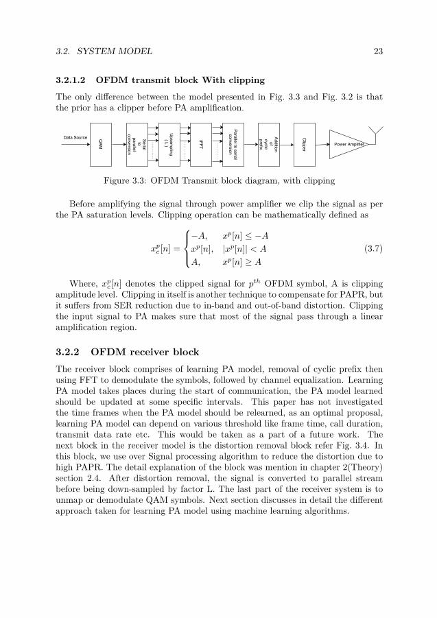
3.2.1.2 OFDM transmit block With clipping
The only difference between the model presented in Fig. 3.3 and Fig. 3.2 is thatthe prior has a clipper before PA amplification.
Figure 3.3: OFDM Transmit block diagram, with clipping
Before amplifying the signal through power amplifier we clip the signal as perthe PA saturation levels. Clipping operation can be mathematically defined as
xpc [n] =
−A, xp[n] ≤ −Axp[n], |xp[n]| < A
A, xp[n] ≥ A(3.7)
Where, xpc [n] denotes the clipped signal for pth OFDM symbol, A is clippingamplitude level. Clipping in itself is another technique to compensate for PAPR, butit suffers from SER reduction due to in-band and out-of-band distortion. Clippingthe input signal to PA makes sure that most of the signal pass through a linearamplification region.
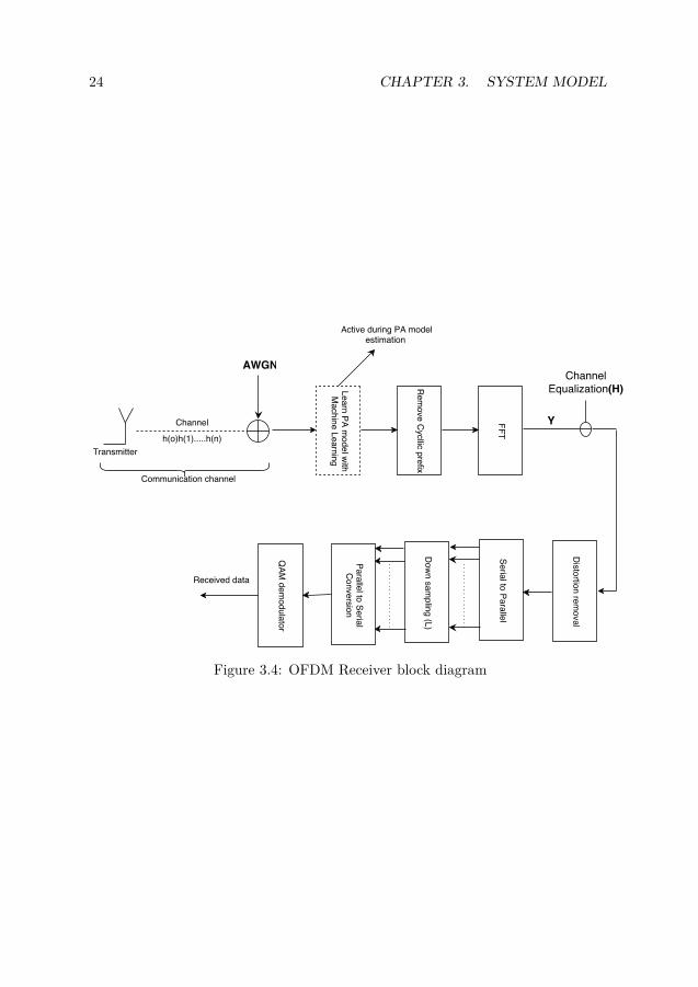
3.2.2 OFDM receiver blockThe receiver block comprises of learning PA model, removal of cyclic prefix thenusing FFT to demodulate the symbols, followed by channel equalization. LearningPA model takes places during the start of communication, the PA model learnedshould be updated at some specific intervals. This paper has not investigatedthe time frames when the PA model should be relearned, as an optimal proposal,learning PA model can depend on various threshold like frame time, call duration,transmit data rate etc. This would be taken as a part of a future work. Thenext block in the receiver model is the distortion removal block refer Fig. 3.4. Inthis block, we use over Signal processing algorithm to reduce the distortion due tohigh PAPR. The detail explanation of the block was mention in chapter 2(Theory)section 2.4. After distortion removal, the signal is converted to parallel streambefore being down-sampled by factor L. The last part of the receiver system is tounmap or demodulate QAM symbols. Next section discusses in detail the differentapproach taken for learning PA model using machine learning algorithms.
24 CHAPTER 3. SYSTEM MODEL
Figure 3.4: OFDM Receiver block diagram
3.2. SYSTEM MODEL 25
3.2.3 Learning the PA model with machine learningThe most novel approach in this thesis is to mitigate the distortion at the receiver,for this, we need to learn the PA model at the receiver. To learn a model we needto train the Machine learning algorithm with a proper set of data. At the start ofthe communication the transmitter sends a set of QAM symbols with amplitudesvarying over the wide range of the PA characteristics, thus at the receiver dataacquisition and PA Model learning block (Fig. 3.4) we learn the PA model. Withproper data , we can use different machine learning algorithms to train the modelbefore being used in the distortion reduction process. Let us go through all thedifferent options available for this system block.
Nonlinear regression is a machine learning technique in which we can use to modela nonlinear relationship in the input-output data. The methods depend on para-metric modeling, which models the dependent variables as a function of nonlinearparameters along with the one or more independent variables. The models can beunivariate or multivariate. The model parameters can comprise of any mathemati-cal form like exponential, trigonometric, power or even another nonlinear function.Eq. 3.8 is an example of a multivariate model , where x and β are the independentvariable and output (Y ) is dependent on them. We use iterative algorithms toestimate the model parameters.
Mathematically we can represent a nonlinear regression as
Y = f(x, β) + ε (3.8)
where x is a vector of p predictors, β is a vector of k parameters, f(.) is someknown regression function, and ε is an error term whose distribution may or maynot be normal. [16] . We can relate β as the weights that would be learned by themachine learning model, x being the input vector and ε the bias term. Now ourtask would be to estimate the β using different machine learning algorithms,
• Least square:If Q is the least square cost function of Eq. 3.8, we can write
Q =n∑i=1
(yi − (fi(x, β))2 (3.9)
Now we need to estimateβ = argmin
βQ (3.10)
We can use different available machine learning algorithms like
In our simulation, we have used smoothing spline and polynomial fit to learnthe model. Let us have a look at these two specific techniques.
3.2.3.2 Smoothing spline
The smoothing spline is a method of fitting a smooth curve to a set of noisy dataset. If we have (xi, yi) as set of observations of various i, the smoothing spline isaimed at finding f(x) of the function f(x) such that
p∑i
wi(yi − f(x))2 + (1− p)∫
(d2f(x)dx2 )2dx (3.11)
is minimum. In our model, function f(x) represents the Solid state PA model givenby Eq. 2.9. The value of p is specified between 0 and 1. When p ≈ 0 but not exactly0, then Eq. 3.11 gives a straight line least square fit to the data. On the other handp=1 will give a spline interpolant. It might not be wrong to consider smoothingspline as parametric regression since we need to specify a value to the parameter p.However, smoothing splines are piecewise polynomial fit and can also be consideredas non parametric. For extensive details on spline function and its curve fittingcapability, on can refer to [17, chapter 13]. The value of p determine how close thefit lies to data, a higher value is closer to data and a lower value is smoother buta bit away from data. The choice of the smoothing spline for learning a PA modellies in the fact that we want a very close fit to the PA. The output from the PAis linear in most of the range thus a value close to 0 would give a smoother leastsquare fit at the same time incorporate the nonlinear fit at higher values(valuesbeyond saturation). In the results section i.e. chapter 5, we have used a small pvalue and varied the number of data points to learn the PA model, the output is asmoother and close to real fit.
3.2.3.3 Polynomial fit
Polynomial regression models are used to fit nonlinear relationship between theinput and output variables eg. function of the form y = f(x). Even thoughpolynomial regression fits a nonlinear function to the data, it is linear in the sensethat the regression function is linear in the unknown parameters estimated fromthe data. we can model a polynomial fit as
The Eq. 3.12 is linear in terms of the unknown values (p0, p1, p2, ...). Thus forthe least square analysis we can use multiple regression to estimate the values of
3.2. SYSTEM MODEL 27
(p0, p1, p2, ...). In a multiple regression model we can calculate the residual sum ofsquare(RSS) as
RSS(P ) =N∑i=1
(Yi − FT (xi)P )2 (3.13)
where Y is the output vector, FT (xi)P is the estimated Yi and P is the weightvector to be evaluated. We can minimize the RSS to calculate the values of theparameters p using any of the machine learning algorithms like gradient descent,Gauss-Newton etc. Polynomial fit forms the simple case of parametric model esti-mation. Polynomial fit is not a very good choice as it becomes unstable at higherdegree but in our simulation scenario it works well, this can be justified from thefact that we that the data collected during training has enough points to reduceextrapolation and give a fast convergence. The ideal PA model to which we aretrying to fit our polynomial has no infliction it increases in the values of interest,thus polynomial fit gives a stable and smooth estimated model for PA.
The main difference between parametric and non parametric regression is the priorknowledge of function being estimated. In a non parametric regression we stillmodel the function but the parameters are very broad, most of the parameters beingunknown or does not have any physical meaning in relation to the problem underconsideration, in contrast, the parametric model has a small number of parametersand has viable meaning with respect to the problem being considered.
Neural networks(NN) comes under the nonparametric models in which thelearned weights of the hidden neurons have no physical meaning for the prob-lem under consideration. The main aim of training a neural network is not mereapproximating the weights (as in parametric models) but to estimate the wholefunction. The distortion algorithm (refer section 2.4.1) requires the knowledge ofthe PA model at the transmitter. In this project we will be using feedforward neuralnetwork for estimating the PA characteristic model at the receiver.
Let us try to understand the working of a neural network and advantage of usingit as a universal appropriator, a NN can realize an arbitrary mapping of one vectorspace onto another vector space [18]. Learning of the weights of NN is consideredas the training process, there are main two types of training process: supervisedand unsupervised training. Supervised training, means that the NN has knowledgeof the desired output and adjusts the weights accordingly eg. feedforward neuralnetwork. On the other hand, in an unsupervised learning, the NN does not haveknowledge about the desired output rather it recognizes a pattern and optimizedto a certain functional relationship. In our PA model estimation requirement, wedo know the desired output values thus a multilayer feedforward networks is a rightchoice.
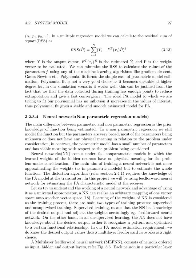
A Multilayer feedforward neural network (MLFNN), consists of neurons orderedas input, hidden and output layers, refer Fig. 3.5. Each neuron in a particular layer
28 CHAPTER 3. SYSTEM MODEL
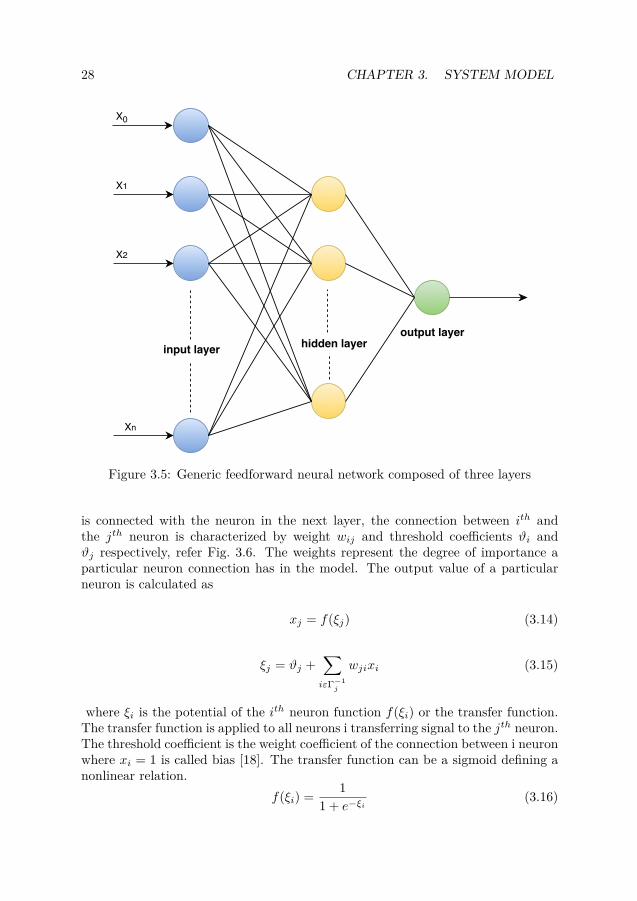
Figure 3.5: Generic feedforward neural network composed of three layers
is connected with the neuron in the next layer, the connection between ith andthe jth neuron is characterized by weight wij and threshold coefficients ϑi andϑj respectively, refer Fig. 3.6. The weights represent the degree of importance aparticular neuron connection has in the model. The output value of a particularneuron is calculated as
xj = f(ξj) (3.14)
ξj = ϑj +∑iεΓ−1
j
wjixi (3.15)
where ξi is the potential of the ith neuron function f(ξi) or the transfer function.The transfer function is applied to all neurons i transferring signal to the jth neuron.The threshold coefficient is the weight coefficient of the connection between i neuronwhere xi = 1 is called bias [18]. The transfer function can be a sigmoid defining anonlinear relation.
f(ξi) = 11 + e−ξi
(3.16)
3.2. SYSTEM MODEL 29
Figure 3.6: Connection between neurons
In the feedforward network supervised training process, the threshold coefficientsϑj and weight coefficient wji are varied to minimize the sum of squares differencebetween actual output and desired output. We can write the minimizing costfunction as
Q =∑j
(xj − xj)2 (3.17)
where xj and xj are the vectors of desired output and actual output run over all j.There can be different training algorithms to calculate the weights and thresholdvalues. One of the most used algorithms is the back-propagation, for a detailedexplanation you can refer [18].
.
Chapter 4
Results
In this section we will discuss the IFB simulation results. The two scenarios underconsiderations are the nonlinearity distortion due to clipping plus PA and the otherone being the distortion only due to PA. Before describing the implementationmethod, let us go through the simulation assumptions and tools used in the project.
4.1 Simulation assumption
We assume that the channel state information is perfectly known at the receiver.The mobile is stationary w.r.t the base station i.e. no Doppler effect in the systemmoreover there is perfect frequency and time synchronization. The simulation sys-tem is designed as a single path but it can be extended and simulated for multipathscenarios. For fast prototyping we have ignored the channel(H) (refer Fig. 2.2) dur-ing training phase of the PA model, moreover we train the PA at high SNR(25dB inthis case) so to have a less noisy training data. MATLAB version R2015a on a Win-dows 7 machine with Intel(R) core(TM) i7-4790s [email protected] is being used for allsimulation, the basic digital communication components are used from MATLABinbuilt functions available in communication tool box. The Curve Fitting tool-box and Neural Network toolbox was used for fast implementation of the differentmachine learning algorithms. It is very much possible to implement and simulatethe system model in this project using Python(Numpy, SciPy libraries) and opensource machine learning libraries like TensorFlow and Microsoft cognitive toolkit(CNTK), which are available on Github.
4.2 Estimation of PA model with machine learning
The first most important block in the receiver is the estimation of PA model, wewill use machine learning algorithms to estimate the PA, the big question thatarises is which algorithm? We have to estimate the model in least estimation timeand the same the symbol error rate(SER) should show improvement with respect
31
32 CHAPTER 4. RESULTS
to non algorithmic case. There are numerous machine learning algorithms that canbe used to estimate the PA model with the available data. All the different modelsare suited in different scenarios and requirement conditions, some of the importantproperties to be considered while selecting a learning method are
1. Training time.
2. Amount of data available.
3. Acceptable Training error.
4. Acceptable Validation error.
0 0.5 1 1.5 2 2.5 3 3.5 4 4.5 5
Input Amplitude
0
0.5
1
1.5
2
2.5
3
3.5
4
4.5
5
Ou
tpu
t A
mp
litu
de
AM/AM response of power amplifier
Linear Response
Amplifier Response
Mean of OFDM Amplitude
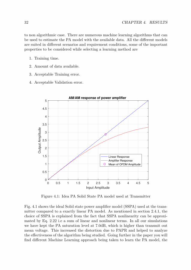
Figure 4.1: Idea PA Solid State PA model used at Transmitter
Fig. 4.1 shows the ideal Solid state power amplifier model (SSPA) used at the trans-mitter compared to a exactly linear PA model. As mentioned in section 2.4.1, thechoice of SSPA is explained from the fact that SSPA nonlinearity can be approxi-mated by Eq. 2.22 i.e a sum of linear and nonlinear terms. In all our simulationswe have kept the PA saturation level at 7.0dB, which is higher than transmit outmean voltage. This increased the distortion due to PAPR and helped to analyzethe effectiveness of the algorithm being studied. Going further in the paper you willfind different Machine Learning approach being taken to learn the PA model, the
4.2. ESTIMATION OF PA MODEL WITH MACHINE LEARNING 33
performance have been tabulated to make easy comparison. We mentioned aboutthese algorithms while describing them in section 3.2.3. The final goal is to findthe best algorithm suited for the particular scenario of any communication systembeing designed. Learning time and accuracy of the learned model to the ideal oneat transmitter are very important for IFB algorithm to give positive results.
4.2.1 Nonlinear regression and piece wise polynomial fitIn this section we have used the nonlinear regression models to estimate the PAat the receiver. Table. 4.1 shows the different setups we experimented to generatethe PA model using smoothing spline. The training data was accumulated at SNR25dB
Table 4.1: Smoothing Spline
Learning AlgorithmTraining Algo-rithm
Data required Trainingtime
Goodness of Fit
SmoothingSpline,p=0.0098
2000x612No. of OFDM Symbols: 2000
No of subcarriers: 512cyclic prefix:100
≤ 40min. SSE: 537.1R-square: 0.9997
Adjusted R-square: 0.9997RMSE: 0.02095
SmoothingSpline,p=0.0098
300x612No. of OFDM Symbols: 300
No of subcarriers: 512cyclic prefix:100
≤1.94min.
SSE: 55.84R-square: 0.9997
Adjusted R-square: 0.9997RMSE: 0.02100
SmoothingSpline,p=0.0098
200x612No. of OFDM Symbols: 200
No of subcarriers: 512cyclic prefix:100
≤1.00min.
SSE: 54.84R-square: 0.9997
Adjusted R-square: 0.9997RMSE: 0.02117
In Table. 4.1, the column goodness of fit, shows all the, this can be a researchto study. qualitative parameters we used for comparing a set of model fits. Let usunderstand how these parameters are evaluated
1. Sum of squares due to error (SSE): This statistic measures the total deviationof the response values from the fit to the response values. Mathematically itis defined as
SSE =n∑i=1
wi(yi − yi)2 (4.1)
where, yi is the actual output and yi is the predicted output by the model.SSE is also called the summed square of residuals, a value closer to 0 indicatesthat the model has a smaller random error component, and that the fit willbe more useful for prediction.
34 CHAPTER 4. RESULTS
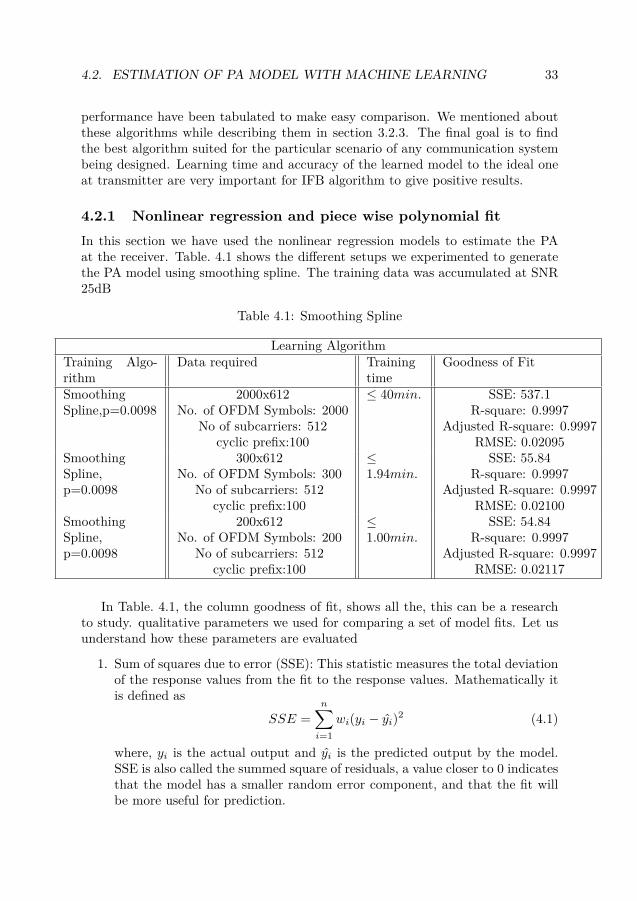
Figure 4.2: PA fit using Smoothing spline
2. R-Square: This statistic measures how successful the fit is in explaining thevariation of the data. Put another way, R-square is the square of the correla-tion between the response values and the predicted response values. It is alsocalled the square of the multiple correlation coefficient and the coefficient ofmultiple determination. R-squared can be defined as the percentage of the re-sponse variable variation that is explained by a linear model. In other words,
R− square = Explained variationTotal variation
=∑ni=1 wi(yi − yi)2∑ni=1 wi(yi − yi)2
(4.2)
where, yi is the actual output, yi is the predicted output by the model andyi is the average of output. R-square can take on any value between 0 and1, with a value closer to 1 indicating that a greater proportion of variance isaccounted for by the model. For example, an R-square value of 0.997 meansthat the fit explains 99.70% of the total variation in the data about the average
3. Degrees of Freedom Adjusted R-Square: This statistic uses the R-squarestatistic defined above, and adjusts it based on the residual degrees of free-dom. The residual degrees of freedom is defined as the number of response
4.2. ESTIMATION OF PA MODEL WITH MACHINE LEARNING 35
values n minus the number of fitted coefficients m estimated from the re-sponse values. ν = n − m, ν indicates the number of independent piecesof information involving the n data points that are required to calculate thesum of squares. Note that if parameters are bounded and one or more ofthe estimates are at their bounds, then those estimates are regarded as fixed.The degrees of freedom is increased by the number of such parameters. Theadjusted R-square statistic can take on any value less than or equal to 1, witha value closer to 1 indicating a better fit. Negative values can occur when themodel contains terms that do not help to predict the response.
4. Root Mean Squared Error: This statistic is also known as the fit standarderror and the standard error of the regression. It is an estimate of the standarddeviation of the random component in the data, and is defined as
RMSE = s = 2√MSE (4.3)
where MSE is the mean square error or the residual mean square
MSE = SSE
ν(4.4)
Just as with SSE, an MSE value closer to 0 indicates a fit that is more usefulfor prediction.
Fig. 4.2 shows the fit generated from Smoothing spline with f(x) = piece wisepolynomial computed from p, where x is normalized by mean 2.875 and std 1.498and Smoothing parameter p = 0.0098. The fit for different iteration are tabulatedin Table. 4.1. When we run the algorithm with 10× less data the plot is exactlysame with very minute change in RMSE error. On a windows system with Inter i7CPU, and using MATLAB (refer section 4.1) curve fitting tool the learning timereduces to less than a minute for 200 OFDM symbols. This time can go signifi-cantly lower with more powerful machine, which justifies a possibility to use thealgorithms in base station radios. Over all smoothing spline proves to be a goodoption for our IFB algorithm when we have less training time, later in the chapteryou will find SER evaluations for different learning algorithms.
36 CHAPTER 4. RESULTS
Table 4.2: Polynomial fit
Learning AlgorithmTraining Algo-rithm
Data required Trainingtime
Goodness of Fit
Linear modelPoly5
2000x612No. of OFDM Symbols: 2000
No of subcarriers: 512cyclic prefix:100
0.5min. SSE: 565.5R-square: 0.9997
Adjusted R-square: 0.9997RMSE: 0.02149
Linear modelPoly5
200x612No. of OFDM Symbols: 200
No of subcarriers: 512cyclic prefix:100
≤0.2min.
SSE: 56.34R-square: 0.9997
Adjusted R-square: 0.9997RMSE: 0.02156
Figure 4.3: PA fit Polynomial fit
Fitting the data on polynomial is a also is good option, with very less data thePA model is approximated pretty much accurately. The polynomial fit can be usedwhen we have very less training time. The Fig. 4.3 shows the fit on a polynomialof degree 5, the parameters being
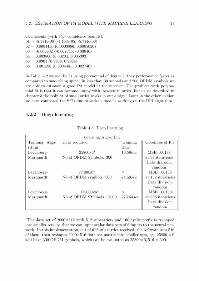
In Table. 4.2 we see the fit using polynomial of degree 5, they performance faster ascompared to smoothing spine. In less than 30 seconds and 200 OFDM symbols weare able to estimate a good PA model at the receiver. The problem with polyno-mial fit is that it can become lumpy with increase in order, but as we described inchapter 3 the poly fit of small order works in our design. Later in the other sectionwe have compared the SER due to various models working on the IFB algorithm.
∗The data set of 2000×612 with 512 subcarriers and 100 cyclic prefix is reshapedinto smaller sets, so that we can input scalar data sets of 6 inputs to the neural net-work. In this implementation, out of 612 sub carries received, the software uses 516of them, then reshapes 2000×516 data set matrix into smaller sets, eg. 25800 × 6will have 300 OFDM symbols, which can be evaluated as 25800×6/516 = 300.
38 CHAPTER 4. RESULTS
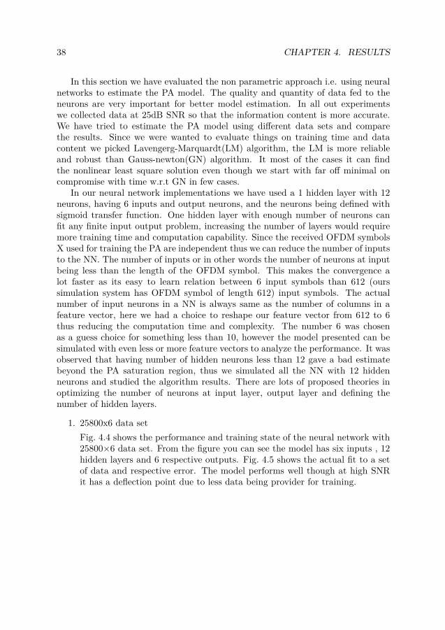
In this section we have evaluated the non parametric approach i.e. using neuralnetworks to estimate the PA model. The quality and quantity of data fed to theneurons are very important for better model estimation. In all out experimentswe collected data at 25dB SNR so that the information content is more accurate.We have tried to estimate the PA model using different data sets and comparethe results. Since we were wanted to evaluate things on training time and datacontent we picked Lavengerg-Marquardt(LM) algorithm, the LM is more reliableand robust than Gauss-newton(GN) algorithm. It most of the cases it can findthe nonlinear least square solution even though we start with far off minimal oncompromise with time w.r.t GN in few cases.
In our neural network implementations we have used a 1 hidden layer with 12neurons, having 6 inputs and output neurons, and the neurons being defined withsigmoid transfer function. One hidden layer with enough number of neurons canfit any finite input output problem, increasing the number of layers would requiremore training time and computation capability. Since the received OFDM symbolsX used for training the PA are independent thus we can reduce the number of inputsto the NN. The number of inputs or in other words the number of neurons at inputbeing less than the length of the OFDM symbol. This makes the convergence alot faster as its easy to learn relation between 6 input symbols than 612 (ourssimulation system has OFDM symbol of length 612) input symbols. The actualnumber of input neurons in a NN is always same as the number of columns in afeature vector, here we had a choice to reshape our feature vector from 612 to 6thus reducing the computation time and complexity. The number 6 was chosenas a guess choice for something less than 10, however the model presented can besimulated with even less or more feature vectors to analyze the performance. It wasobserved that having number of hidden neurons less than 12 gave a bad estimatebeyond the PA saturation region, thus we simulated all the NN with 12 hiddenneurons and studied the algorithm results. There are lots of proposed theories inoptimizing the number of neurons at input layer, output layer and defining thenumber of hidden layers.
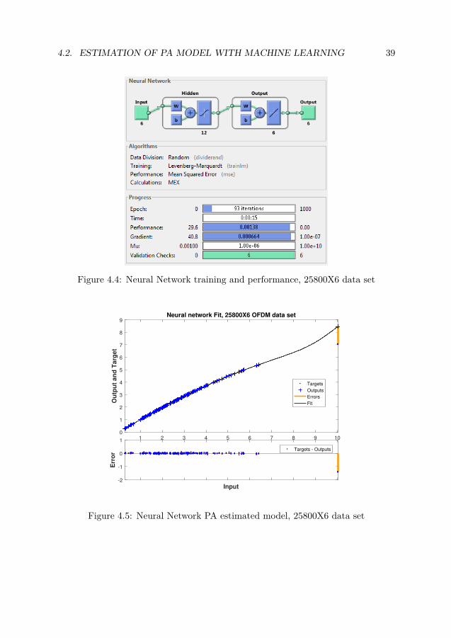
1. 25800x6 data setFig. 4.4 shows the performance and training state of the neural network with25800×6 data set. From the figure you can see the model has six inputs , 12hidden layers and 6 respective outputs. Fig. 4.5 shows the actual fit to a setof data and respective error. The model performs well though at high SNRit has a deflection point due to less data being provider for training.
4.2. ESTIMATION OF PA MODEL WITH MACHINE LEARNING 39
Figure 4.4: Neural Network training and performance, 25800X6 data set
1 2 3 4 5 6 7 8 9 100
1
2
3
4
5
6
7
8
9
Ou
tpu
t an
d T
arg
et
Neural network Fit, 25800X6 OFDM data set
Targets
Outputs
Errors
Fit
Input-2
-1
0
1
Err
or
Targets - Outputs
Figure 4.5: Neural Network PA estimated model, 25800X6 data set
40 CHAPTER 4. RESULTS
2. 77400x6 data set
Figure 4.6: Neural Network training and performance, 77400X6 data set
1 2 3 4 5 6 7 8 9 100
1
2
3
4
5
6
7
8
Ou
tpu
t an
d T
arg
et
Neural Network Fit, 77400X6 OFDM data set
Targets
Outputs
Errors
Fit
Input-0.2
0
0.2
Err
or
Targets - Outputs
Figure 4.7: Neural Network PA estimated model, 77400X6 data set
Fig. 4.6 shows the training and performance state of model with 77400×6 data
4.2. ESTIMATION OF PA MODEL WITH MACHINE LEARNING 41
set. It takes a little more time and iterations to train the model but whenyou compare Fig. 4.7 with Fig. 4.5, you can clearly see that the prior givesa good fit even at higher SNR. This is mainly due to the fact that providingmore data to the neurons help them recognize the model pattern throughoutthe SNR variation.
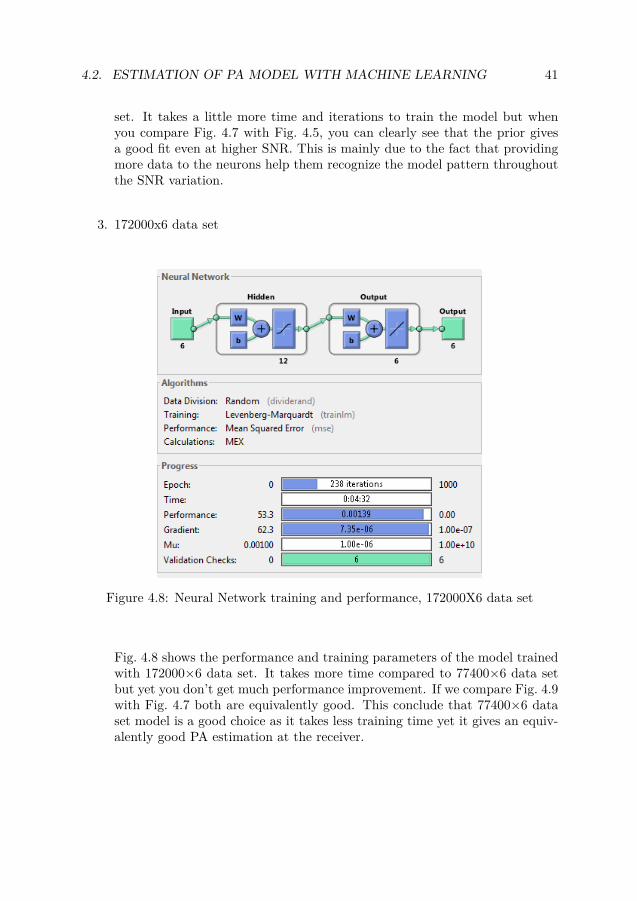
3. 172000x6 data set
Figure 4.8: Neural Network training and performance, 172000X6 data set
Fig. 4.8 shows the performance and training parameters of the model trainedwith 172000×6 data set. It takes more time compared to 77400×6 data setbut yet you don’t get much performance improvement. If we compare Fig. 4.9with Fig. 4.7 both are equivalently good. This conclude that 77400×6 dataset model is a good choice as it takes less training time yet it gives an equiv-alently good PA estimation at the receiver.
42 CHAPTER 4. RESULTS
1 2 3 4 5 6 7 80
1
2
3
4
5
6
7O
utp
ut
an
d T
arg
et
Neural network Fit, 172000x6 OFDM data set
Targets
Outputs
Errors
Fit
Input-0.1
0
0.1
Err
or
Targets - Outputs
Figure 4.9: Neural Network PA estimated model, 172000X6 data set
4.2.3 Distortion due to PA nonlinearity
In this section we will consider such a scenario and analyze the performance of theIFB algorithm, when there is distortion only due to power amplifier.
4.2.3.1 Symbol Error Rate
Table 4.4: Simulation parameter, distortion due to PA nonlinearity
System Simulation ParametersNumber of transmitted OFDMSymbols
200∗
Modulation Type 64-QAMNumber of Subcarriers 512Number of Cyclic prefix 100PA Saturation level(dB) 7.0Signal Clipping(dB) No clipping
4.2. ESTIMATION OF PA MODEL WITH MACHINE LEARNING 43
∗Note that these are the number of OFDM symbols used to transmit informationdata during simulation, the number of symbols used for training the PA modeldiffers, smoothing spline was trained with 300 OFDM symbols, Poly5 model wastrained with 200 OFDM symbols and neural network model was trained with 900symbols. Let us see how the symbol error rate reduces when we apply IFB to
0 5 10 15 20 25
SNR [dB]
10-2
10-1
100
Sym
bo
l E
rro
r R
ate
OFDM Symbol Error Rate vs SNR
Original, No IFB
IFB, PA trained with poly of degree 5
IFB, PA trained with Smoothing Spline
IFB, Exact PA model
IFB, PA trained with Neural network
Figure 4.10: Symbol Error Rate vs SNR for IFB, distortion due to PA nonlinearity,PA Saturation 7.0dB
the OFDM system without any clipping. In this case we have used the simulationparameters as mentioned in Table. 4.4.
Fig. 4.10 shows the simulation results when there is no clipping of the inputsignal. The nonlinearity distortion is only caused by the Power amplifier gettinginto saturation region. From the plot its very clear that the IFB algorithm stilloutperforms, SER decreases considerably as compared to the non algorithmic case.The red line(IFB, PA trained with Neural network) in Fig. 4.10 shows the SERvariation when we train the receiver PA model using Neural network. The neuralnetwork clearly gives good results at all SNR above 10dB. The next one very closeto the neural network is the PA model fitted with polynomial of degree 5. Theyellow line(IFB, Exact PA model) shows the SER variation when we use the samePA as in the transmitter, good performance of Neural network model can seen asit perform very close to exact PA model. If training time is very important then
44 CHAPTER 4. RESULTS
polynomial fit is definitely a good choice. If we need a robust and better SER at allSNR level then training the PA with deep learning method should be considered.
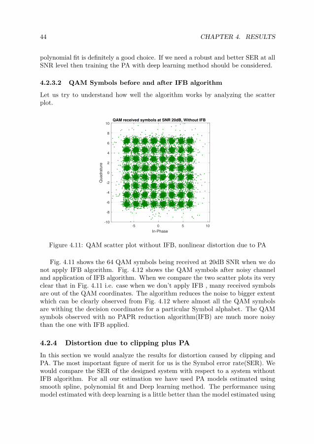
4.2.3.2 QAM Symbols before and after IFB algorithm
Let us try to understand how well the algorithm works by analyzing the scatterplot.
-5 0 5 10
In-Phase
-10
-8
-6
-4
-2
0
2
4
6
8
10
Quadra
ture
QAM received symbols at SNR 20dB, Without IFB
Figure 4.11: QAM scatter plot without IFB, nonlinear distortion due to PA
Fig. 4.11 shows the 64 QAM symbols being received at 20dB SNR when we donot apply IFB algorithm. Fig. 4.12 shows the QAM symbols after noisy channeland application of IFB algorithm. When we compare the two scatter plots its veryclear that in Fig. 4.11 i.e. case when we don’t apply IFB , many received symbolsare out of the QAM coordinates. The algorithm reduces the noise to bigger extentwhich can be clearly observed from Fig. 4.12 where almost all the QAM symbolsare withing the decision coordinates for a particular Symbol alphabet. The QAMsymbols observed with no PAPR reduction algorithm(IFB) are much more noisythan the one with IFB applied.
4.2.4 Distortion due to clipping plus PAIn this section we would analyze the results for distortion caused by clipping andPA. The most important figure of merit for us is the Symbol error rate(SER). Wewould compare the SER of the designed system with respect to a system withoutIFB algorithm. For all our estimation we have used PA models estimated usingsmooth spline, polynomial fit and Deep learning method. The performance usingmodel estimated with deep learning is a little better than the model estimated using
4.2. ESTIMATION OF PA MODEL WITH MACHINE LEARNING 45
-8 -6 -4 -2 0 2 4 6 8
In-Phase
-8
-6
-4
-2
0
2
4
6
8
Quadra
ture
QAM received symbols at SNR 20dB, With IFB
Figure 4.12: QAM scatter plot with IFB, nonlinear distortion due to PA
smooth spine or polynomial fit. It depends on the requirement on training time tochoose the require PA estimation method.
4.2.4.1 Symbol Error Rate
As mentioned earlier the figure of merit for this paper is the reduction in Symbolerror rate at the receiver. For this simulation, error generated by nonlinearity fromPA and clipping we have used the parameters as in Table. 4.5
Table 4.5: Simulation parameter, distortion due to clipping plus PA nonlinearity
System Simulation ParametersNumber of transmitted OFDMSymbols
200∗
Modulation Type 64-QAMNumber of Subcarriers 512Number of Cyclic prefix 100PA Saturation level(dB) 7.0Signal Clipping(dB) ±7.0
∗Note that these are the number of OFDM symbols used to transmit informa-tion data during simulation, the number of symbols used for training the PA modeldiffers, smoothing spline was trained with 300 OFDM symbols, Poly5 model wastrained with 200 OFDM symbols and neural network model was trained with 900
46 CHAPTER 4. RESULTS
symbols.
The IFB algorithm works pretty well with the designed communication system.Fig. 4.13 shows the simulation result.
0 5 10 15 20 25
SNR [dB]
10-2
10-1
100
Sym
bo
l E
rro
r R
ate
OFDM Symbol Error Rate vs SNR
Original, No IFB
IFB, PA trained with Neural network
IFB, PA trained with Poly of degree 5
IFB, PA trained with Smoothing Spline
IFB, Exact PA model
Figure 4.13: Symbol Error Rate vs SNR for IFB, distortion due to clipping plusPA nonlinearity, PA Saturation 7.0dB, clip level 7.0dB
The blue line(Original, No IFB) shows the Symbol error rate(SER) without theIFB algorithm while the yellow line(IFB, Exact PA model) shows SER with IFBand exact transmitter PA model used at receiver. The green line(IFB, PA trainedwith smoothing spline) is the IFB algorithm performance when we train the PAwith smoothing spline. Similarly the black(IFB, PA trained with Poly of degree5) is when we train the PA using polynomial fit of degree 5. It is very interestingto notice that the Smoothing and polynomial fit model performs same at lowerSNR while the red(PA trained with deep learning) outperforms everything else atSNR above 10dB. Deep learning can be a choice when we have SNR variation on abigger intervals else the polynomial fit does the work. One more thing that shouldbe considered while deciding algorithm choice is the training time. A more accuratesmoothing spline needs higher training time.
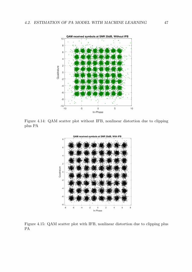
4.2. ESTIMATION OF PA MODEL WITH MACHINE LEARNING 47
-10 -5 0 5 10
In-Phase
-10
-8
-6
-4
-2
0
2
4
6
8
10
Quadra
ture
QAM received symbols at SNR 20dB, Without IFB
Figure 4.14: QAM scatter plot without IFB, nonlinear distortion due to clippingplus PA
-8 -6 -4 -2 0 2 4 6 8
In-Phase
-8
-6
-4
-2
0
2
4
6
8
Qu
ad
ratu
re
QAM received symbols at SNR 20dB, With IFB
Figure 4.15: QAM scatter plot with IFB, nonlinear distortion due to clipping plusPA
48 CHAPTER 4. RESULTS
4.2.4.2 QAM symbols before and after IFB algorithm
As we compared the QAM in section 4.2.3.2 for clipping plus PA case , in thissection we would analyze the QAM symbol scatter plot when we have distortiondue to PA plus clipping. Fig. 4.14 shows the QAM symbols at 20dB SNR whenthere is no IFB applied to the communication system. When you compare thiswith Fig. 4.15. You can notice that many symbols in Fig. 4.14 is scattered outof the 64 quadrants while in the case when we have the IFB included, almost allthe QAM symbols are close to the quadrants and thus demodulated with less erroralias decrease in symbol error rate.
4.2.5 Symbol Error rate for different PA saturation level
SNR [dB]
0 5 10 15 20 25
Sym
bo
l E
rro
r R
ate
10-3
10-2
10-1
100OFDM Symbol Error Rate vs SNR
PA sat 5dB, IFB, PA trained with Neural network
PA sat 10dB, IFB, PA trained with Neural network
PA sat 7dB, IFB, PA trained with Neural network
PA sat 7dB, No IFB
PA sat 5dB, No IFB
PA sat 10dB, No IFB
Figure 4.16: Symbol Error Rate vs SNR for IFB, distortion due to PA nonlinearity,PA Saturation 10.0dB, 7.0dB and 5.0dB
In this section we have analyzed the variation of symbol error rate for differentPA saturation level when distortion is due to PA nonlinearity, which is similar tothe SER variation with PA plus clipping nonlinearity at different PA saturationlevel. As we increase the PA saturation level SER goes on decreasing, which can be
4.2. ESTIMATION OF PA MODEL WITH MACHINE LEARNING 49
justified from the fact that increasing saturation level leads to an increase in linearoperation range of PA. Fig. 4.16 shows the variation of SER with PA saturationlevel of 10dB, 7dB and 5dB. It can be seen from the Fig. 4.16 that PA 10dB symbolerror rate is lowest as compared to symbol error rate at 7dB and 5dB.
Chapter 5
Conclusions and future works
In this report, we have analyzed an algorithm to reduce the bit errors in an OFDMmodulated system. The two scenarios considered were the nonlinearity distortiondue to clipping plus PA system and the other one when we have system withoutany clipper. In this project we have tried to reduce the nonlinearity at the receiverusing algorithm proposed in [5, 6]. For the same we need to estimate the PA at thereceiver. We used different machine learning algorithms to learn the PA model usingsome training data. We analyzed different machine learning algorithms in section4.2, which showed that different PA learning method is suited for different scenariosdepending on the data available and amount of training time. Later we saw thatdeep learning method gives us really good estimate of the data at little more cost interms of time and CPU memory requirement for estimating the PA model. On theother hand the cost of implementing IFB can been seen as two additional IFFT’sas compared to a model without any distortion compensation(IFB) block, whichmakes it clear that we need additional computation resource to use the projectoutcomes in real world.
The processing capacity of the mobile base stations are very powerful today,applying the deep learning algorithm in this case would give considerable SER re-duction with lesser PA training time. The results prove that if there are constraintswith computation power then other algorithm like smoothing spline and polyno-mial fit is definitely good options for estimating the PA model at the receiver, andthen applying IFB algorithm. Most of the mobile handsets are not that powerfulto implement DPD, in such a scenario the results from this project can be used forPAPR reduction. If we have the IFB algorithm running at both ends of the commu-nication system (i.e the base station and user equipment), there can be much morereliant data transmission. The result in this work proves the usability of machinelearning and signal processing in reducing the distortion due to high PAPR in anOFDM modulated system. As a part of future work we can investigate the per-formance of the proposed algorithm with other machine learning algorithms anddifferent design choices. We can try to reduce the number of neurons and have
51
52 CHAPTER 5. CONCLUSIONS AND FUTURE WORKS
more hidden layers with lesser input-output neurons or even model the PA withlower order polynomial. Another task as a part of future work is to estimate thetime frame in which we need to relearn the PA model inorder to maintain lowerSER. One more interesting work is to compare the performance of the IFB with asystem where we can transmit some additional information to tract the nonlinear-ity like the tone injection(TI) [15]. Such a method would reduce the data rate butwe will gain in term of quality(i.e better SER). Internet of things applications likethe sensor networks has much lower data rate requirements, in such a scenario acompromise in data rate for transmission reliability is well justified.
Bibliography
[1] R. W. Chang, “Synthesis of band-limited orthogonal signals for multichanneldata transmission,” Bell Syst. Tech. J., vol. 45, pp. 1775 – 1796, December1966.
[2] S. Weinstein and P. Ebert, “Data transmission by frequency-division multi-plexing using the discrete fourier transform,” , IEEE Transactions on Com-munications, vol. 19, pp. 628 – 634, October 1971.
[3] H. R. (ed.), OFDM: Concepts for Future Communication Systems. Springer,ISBN: 3642174957, April 2011.
[4] A. R. Bahai and B. R. Saltzberg, Multi-Carrier Digital Communications: The-ory and Applications of OFDM. Plenum Publishing Corp., October 1999.
[5] F. H. Gregorio, S. Werner, J. Cousseau, J. Figueroa, and R. Wichman,“Receiver-side nonlinearities mitigation using an extended iterative decision-based technique,” Signal Processing, vol. 91, pp. 2042–2056, 2011.
[6] J. tellado, L. M. C. Hoo, and J. M. Cioffi, “Maximum-likelihood detectionof nonlinearly distorted multicarrier symbols by iterative decoding,” IEEETransactions on communications, vol. 51, no. 2, 2003.
[7] H. E. Rowe, “Memoryless nonlinearities with gaussian inputs: elementary re-sults,” The bell system technical , journal, vol. 61, no. 7, September 1982.
[8] T. Schenk, RF-Imperfections in High-rate Wireless System, Impact and DigitalCompensation. Springer, ISBN: 978-1-4020-6903-1.
[9] A. N. D. Andrea, V. Lottici, and R. Reggiannini, “Rf power amplifier lin-earization through amplitude and phase predistortion,” IEEE transactions oncommunications,, vol. 44, no. 11, November 1996.
[10] R. Marsalek, P.Jaedin, and G. Baudoin, “From post-distortion to predistortionfor power amplifier linearization,” IEE communication letters, vol. 7, no. 7,2003.
53
54 BIBLIOGRAPHY
[11] A. N.D’Andrea, V. Lottici, and R. Regiannini, “Nonlinear predistortion ofofdm signals over frequency-selective fading channels,” IEE transaction oncommunication, vol. 49, no. 7, 2001.
[12] A. A. M. Saleh, “Frequency-independent and frequency-dependent nonlinearmodels of twt amplifiers,” IEE transaction on communication, vol. 29, no. 11,1981.
[13] I. Sohn, “A low complexity papr reduction scheme for ofdm systems via neuralnetworks,” IEEE Communication Letters, vol. 18, no. 2, 2014.
[14] M. Friese, “On the degradation of ofdm-signals due to peak-clipping in opti-mally predistorted power amplifiers,” IEEE Global Telecommunications Con-ference, 1998. GLOBECOM 1998. The Bridge to Global Integration., vol. 2,pp. 939 – 944, November 1998.
[15] J. Tellado, Peak Power Reduction for Multicarrier Transmission. PhD thesis,Stanford University, 2000.
[16] M. H. Kutner, C. J. Nachtsheim, and J. Neter, “Applied linear regressionmodels, fourth edition,” McGraw-Hill Companies, p. chapter 15.5, 2003.
[17] P. eggermont and V. LaRiccia, Maximum penalized likelihood estimation, Vol-ume II-Regression. Springer series in statistic, ISBN: 978-0-387-40267-3, 2004.
[18] D. Svozil, V. kvasnicka, and jiri pospichal, “Introduction to multi-layer feed-forward neural networks,” Chemometrics and Intelligent Laboratory Systems,Elsevier Science B.V., vol. 39, pp. 43–62, November 1997.