Machine Learning for the Detection of Oil Spills in ...1007452223027.pdf · Machine Learning for...

Machine Learning, 30, 195–215 (1998)c© 1998 Kluwer Academic Publishers, Boston. Manufactured in The Netherlands.

Machine Learning for the Detection of Oil Spills inSatellite Radar Images

MIROSLAV KUBAT* [email protected]

ROBERT C. HOLTE [email protected]

STAN MATWIN [email protected]

School of Information Technology and Engineering, University of Ottawa, 150 Louis Pasteur, OttawaOntario, K1N 6N5 Canada

Editors: Ron Kohavi and Foster Provost

Abstract. During a project examining the use of machine learning techniques for oil spill detection, we encounteredseveral essential questions that we believe deserve the attention of the research community. We use our particularcase study to illustrate such issues as problem formulation, selection of evaluation measures, and data preparation.We relate these issues to properties of the oil spill application, such as its imbalanced class distribution, thatare shown to be common to many applications. Our solutions to these issues are implemented in the CanadianEnvironmental Hazards Detection System (CEHDS), which is about to undergo field testing.

Keywords: Inductive learning, classification, radar images, methodology

1. Introduction

In this paper we describe an application of machine learning to an important environmentalproblem: detection of oil spills from radar images of the sea surface. We cover the applica-tion cycle from the problem formulation phase to the delivery of a system for field testing.The company that sponsored this work, Macdonald Dettwiler Associates, has just begunthe final phases of the cycle—field testing, marketing, and deployment. This paper focuseson the research issues that arose during the development of the Canadian EnvironmentalHazards Detection System (CEHDS). These issues cover the entire gamut of activities re-lated to machine learning, from initial problem formulation, through methodology design,to the usual technical activities. For most of the issues, including the technical ones, wefound few pertinent studies in the research literature. The related work we did find wasusually by others working on a particular application. The primary purpose of this paperis to present to the machine learning research community a set of open research issues thatare of general importance in machine learning applications. We also present the approachtaken to these issues in our application.

* Current affiliation/address: Center for Advanced Computer Studies, The University of Southwestern Louisiana,Lafayette, LA 70504-4330, and Computer Science Department, Southern University at Baton Rouge, Baton Rouge,LA 70813-0400, U.S.A., [email protected]

196 M. KUBAT, R. HOLTE, AND S. MATWIN

Figure 1. An example of a radar image of the sea surface

1.1. The Application Domain

Only about 10% of oil spills originate from natural sources such as leakage from sea beds.Much more prevalent is pollution caused intentionally by ships that want to dispose cheaplyof oil residues in their tanks. Radar images from satellites such asRADARSAT andERS-

1 provide an opportunity for monitoring coastal waters day and night, regardless of weatherconditions. Oil slicks are less reflective of radar than the average ocean surface, so theyappear dark in an image. An oil slick’s shape and size vary in time depending on weatherand sea conditions. A spill usually starts out as one or two slicks that later break up intoseveral smaller slicks. Several natural phenomena (e.g., rain, algae) can closely resembleoil slicks in radar images. They are calledlookalikes.

Figure 1 shows a fragment of aSAR (Synthetic Aperture Radar) image of the NorthSea with an oil slick in it. The full image consists of 8,000x8,000 pixels, with each pixelrepresenting a square of 30x30m; the fragment shown here is approximately70 × 50kilometers. The oil slick is the prominent elongated dark region in the upper right of thepicture. The dark regions in the middle of the picture and the lower left are lookalikes, mostprobably wind slicks (winds with speeds exceeding 10m/sec decrease the reflectance of theradar, hence the affected area looks darker in a radar image).

1.2. Previous Work on Oil Spill Detection

Since the early days of satellite technology andSAR there have been attempts to detect oilspills from radar images. The state of the art is represented by the preoperational servicefor identifying oil spills inERS-1 images that has been offered since 1994 by the Tromsø

DETECTION OF OIL SPILLS 197

Satellite Station (TSS) in Norway. This service is entirely manual; humans are trained todistinguish oil spills from nonspills in satellite images.TSS recognizes the desirability ofhaving an automatic system to reduce and prioritize the workload of the human inspectors,and has supported research to develop systems for this purpose. This research has recentlyproduced two systems (Solberg & Solberg, 1996; Solberg & Volden, 1997), but neither hasyet been incorporated intoTSS’s service. Our system was developed in parallel with, andindependently of, these two systems.

The system described by Solberg and Solberg (1996) uses learning to produce a classifier inthe form of a decision tree. As this system is similar to ours in many ways, it will be reviewedin detail in the discussion of our results.TSS’s most recent automatic classification system(Solberg & Volden, 1997) is more knowledge intensive. The classifier is a statistical systemin which the prior probability of a region being an oil spill is computed using a domaintheory that relates features of the region to the prior. The prior is then combined with aGaussian classifier that has been learned from training data. The system performs verywell, correctly classifying 94% of the oil spills and 99% of the nonspills. The system reliesheavily on the knowledge of the wind conditions in the image, and it was necessary fortheTSS team to develop techniques for inferring this from the image. This crucial pieceof information is not available to our system, as we do not at present have methods forinferring wind conditions.

Elsewhere a group of environmental scientists and remote sensing experts have developeda preliminary model of properties of an oil spill image. The model, expressed as a decisiontree (Hovland, Johannessen & Digranes, 1994), uses attributes such as the shape and sizeof the dark regions in the image, the wind speed at the time when the image was taken, theincidence angle of the radar beam, proximity to land, etc. The model has been evaluated onartificial data from a controlled experimental slick, as well as on data from aSAR imageof a real slick. The conclusion was that the model performed well on the artificial data,but was inconsistent with the current physical theory of slick reflectance, and did not agreewith theSAR images.

A similar problem of classification of ice imagery into age groups has received attentionin the image processing and remote sensing literature. Heerman and Khazenie (1992) useda neural network trained by backpropagation to classify Arctic ice into “new” and “old.”Haverkamp, Tsatsoulis and Gogineni (1994) developed a rule based expert system in whichthe rules were acquired from experienced human experts. The performance of this systemexceeded by some 10% the accuracy of previous systems which relied on the brightnessof pixels for classification without any use of symbolic features describing higher levelattributes of the classified objects.

2. Task Description

An oil spill detection system based on satellite images could be an effective early warningsystem, and possibly a deterrent of illegal dumping, and could have significant environ-mental impact. Oil spill detection currently requires a highly trained human operator toassess each region in each image. A system that reduced and prioritized the operator’sworkload would be of great benefit, and the purpose of our project was to produce such asystem.CEHDS is not intended for one specific end user. It is to be marketed worldwide


to a wide variety of end users (e.g., government agencies, companies) with different objec-tives, applications, and localities of interest. It was therefore essential that the system bereadily customizable to each user’s particular needs and circumstances. This requirementmotivates the use of machine learning. The system will be customized by training on ex-amples of spills and nonspills provided by the user, and by allowing the user to control thetradeoff between false positives and false negatives. Unlike many other machine learningapplications (e.g., the fielded applications described by Langley and Simon (1995)), wheremachine learning is used to develop a classifier which is then deployed, in our applicationit is the machine learning algorithm itself that will be deployed.

The input toCEHDS is a raw pixel image from a radar satellite. Image processingtechniques are used to normalize the image in certain ways (e.g., to correct for the radarbeam’s incidence angle), to identify suspicious dark regions, and to extract features (e.g.,size, average brightness) of each region that can help distinguish oil spills from lookalikes.This part of the system was developed by Macdonald Dettwiler Associates, a companyspecializing in remote sensing and image processing. The output of the image processingis a fixed-length feature vector for each suspicious region. During normal operation, thesefeature vectors are fed into a classifier to decide which images, and which regions within animage, to present for human inspection. The operator then makes the final decision aboutwhat response is appropriate.

The classifier is created by the learning algorithm distributed as part ofCEHDS. It isthe development of this learning system that is the focus of this paper. The learner’s inputis the set of feature vectors describing the dark regions produced by the image processingsubsystem. During training the regions are classified by a human expert as oil slicks andlookalikes. These classifications are imperfect. On some occasions, the expert was not quitesure whether or not the region was an oil slick, and the class labels can thus be erroneous.The learner’s output is a classifier capable of deciding whether or not a specific dark regionis an oil spill.

The system’s interface was determined primarily by the requirements set by MacdonaldDettwiler Associates. Early in the design process it was decided that a unit of outputwill be a satellite image, with the regions classified as spills highlighted with a coloredborderline. The total number of images presented for inspection must not be too large. Onthe other hand, the fewer images presented, the greater the risk that an actual oil slick willbe missed. Users should therefore have control over the system, so they can easily vary thenumber of images presented to them. The classifier should be provided with a parameterwhose one extreme value ensures that the user sees all images (no matter whether theycontain oil slicks or not), and whose other extreme value totally blocks the inspection.The intermediate values represent the degree of “confidence” the system must have in theclassification of a particular region before the entire image containing the region will bepresented for inspection. When an image is presented, the system highlights all the regionsin it whose likelihood of being a spill exceeds the parameter value. Learning is not requiredto be rapid or incremental; training data that becomes available in the future may be usedto create a new training set so that the system can induce a new classifier.


3. Key Problem Characteristics

In developing the machine learning component of the system, the main design decisionswere critically affected by certain key features of the oil spill detection problem. Many(though not all) of these features concern characteristics of the oil slick data. Brodley andSmyth (1995) refer to these aspects of a system’s design as “application factors.”

The first critical feature is thescarcityof data. Although satellites are continually pro-ducing images, most of these images contain no oil spills, and we did not have access toan automatic system for identifying those that do (theTSS data and systems reported bySolberg and collaborators were produced in parallel with our project and, in addition, areproprietary). A human expert therefore has to view each image, detect suspicious regions,and classify these regions as positive and negative examples. In addition to the genuineinfrequency of oil spills and the limited time of the expert, the data available is restricted byfinancial considerations: images cost hundreds, sometimes thousands of dollars each. Wecurrently have 9 carefully selected images containing a total of 41 oil slicks. While manyapplications work with large amounts of available data (Catlett, 1991), our domain applica-tion is certainly not unique in its data scarcity. For example, in the drug activity applicationreported by Dietterich, Lathrop and Lozano-Perez (1997) the two datasets contain 47 and39 positive examples respectively.

The second critical feature of the oil spill domain can be called animbalanced training set:there are very many more negative examples (lookalikes) than positive examples (oil slicks).Against the 41 positive examples we have 896 negative examples; the majority class thuscomprises almost 96% of the data. Highly imbalanced training sets occur in applicationswhere the classifier is to detect a rare but important event, such as fraudulent telephone calls(Fawcett & Provost, 1997), unreliable telecommunications customers (Ezawa, Singh &Norton, 1996), failures or delays in a manufacturing process (Riddle, Segal & Etzioni, 1994),rare diagnoses such as the thyroid diseases in the UCI repository (Murphy & Aha, 1994),or carcinogenicity of chemical compounds (Lee, Buchanan & Aronis, 1998). Extremelyimbalanced classes also arise in information retrieval and filtering tasks. In the domainstudies by Lewis and Catlett (1994), only 0.2% (1 in 500) examples are positive. In thehigh-energy physics learning problem reported by Clearwater and Stern (1991), only 1example in a million is positive.

The third critical feature is that examples are naturally grouped inbatches.The examplesdrawn from the same image constitute a single batch. Whenever data is collected in batches,there is a possibility that the batches systematically differ from one another, or that there isa much greater similarity of examples within a batch than between batches. In our domain,for example, the exact parameter settings of the radar imaging system or low-level imageprocessing are necessarily the same for examples within a batch but could be different fordifferent batches. Clearly, in our case, the classifier will be learned from one set of images,and it will be applied on images that were not part of this set. This fact should be taken intoaccount in the evaluation of the system.

This problem has been mentioned by several other authors, including Burl et al. (1998),Cherkauer and Shavlik (1994), Ezawa et al. (1996), Fawcett and Provost (1997), Kubat,Pfurtscheller and Flotzinger (1994), and Pfurtscheller, Flotzinger and Kalcher (1992). Forinstance, in theSKICAT system (Fayyad, Weir & Djorgovski, 1993), the “batches” were


plates, from which image regions were selected. When the system trained on images fromone plate was applied to images from another plate, the classification accuracy droppedwell below that of manual classification. The solution used inSKICAT was to normalizesome of the original features.

The final critical feature relates to theperformance task.The classifier will be used asa filter—it will decide which images to present to a human. This requirement is quitepervasive in real-world applications. Fraud detection, credit scoring, targeted marketing,evaluation ofEEG signals—all of these domains require that a human expert be able todecide how many “suspicious” cases to pursue. The system must provide the user with aconvenient means of varying “specificity” (higher specificity means fewer false alarms atthe cost of increased risk of missing a genuine oil spill).

4. Problem Formulation Issues

Machine learning research usually assumes the existence of carefully prepared data that isthen subjected only to minor, if any, further processing; an attribute or two might be deleted,missing values filled in, some classes merged or dropped. In applications, the situation isnot that straightforward (Langley & Simon, 1995). In our case we did not have a precisestatement of the problem, much less a data file prepared in a standard format.

This section briefly discusses issues related to problem formulation. Based on the initialvague description of the given problem, a successful designer of a learning system mustmake crucial decisions about the choice of the learning paradigm, about the representationand selection of the training examples, and about the categories into which the examplesare going to be classified.

These choices must be made in all applications and they undoubtedly have a profoundeffect on the success, or appropriateness, of learning. Yet the exact nature of this effect isunknown and a systematic study of these aspects is needed.

1. The first decision concernedgranularity. In our application three different approachesare possible. One of them works with the whole image, and its output simply stateswhether the given image contains an oil slick. The second approach works with thedark regions detected in the images, and provides the user with coordinates of thoseregions that are considered as oil spills. Finally, the third approach classifies individualpixels (“this pixel is part of an oil slick”), for instance as has been done by Ossen,Zamzow, Oswald and Fleck (1994). The approach operating with pixels represents thefinest granularity, whereas the approach operating with images represents the coarsestgranularity.

Finer granularity provides more examples—compare the millions of pixels, with the937 regions and 9 images. Moreover, in our application a higher misclassification ratecan be tolerated at the pixel level. 80% accuracy on the pixels in oil slicks is likely toidentify more than 80% of the oil slicks. On the other hand, pixels can be describedonly with an impoverished set of features, and the result need not necessarily seemcoherent to the user (e.g., if pixels are classified individually there is no guarantee thatthe “oil slick” pixels will form coherent regions in an image). We decided the systemwould classify regions.


Table 1.Confusion matrix

guessed:negative positive

true: negative a bpositive c d

The need to choose the degree of granularity arises naturally in many applications. Forinstance in semiconductor manufacturing (Turney, 1995), circuits are manufacturedin batches of wafers, and the system can be required to classify an entire batch, oreach wafer, or to operate at even lower levels. Likewise, the text-to-speech mappingdiscussed by Dietterich, Hild and Bakiri (1995) can be addressed at four distinct levelsof granularity.

Our decision to classify regions had important consequences for the general designof the system. Together with the granularity of the interface, which according toMacdonald Dettwiler’s requirement was at the image level, it has constrained the optionsconcerning the output of our system. We could not have ranked regions according totheir probability of being an oil spill, because our unit of output was an image. Wecould not have classified images, because our system was to support decisions aboutregions, rather than images.

2. Another question was how many and which categories to define. Should all lookalikesbe treated as a single category? Does it make sense to establish separate categories fordifferent kinds of lookalikes? Discussions with the expert who classified the trainingexamples have revealed that she might be able to place many lookalikes into subcat-egories like rain cells, wind, ship wakes, schools of herrings, red tide (plankton) andsome others. Information about which categories are more prone to be misclassifiedcould provide us with a clue for a better choice of training examples. Unfortunately,we overlooked this possibility during the initial data collection and so have been forcedto have just one nonspill class. Solberg and Solberg (1996) divide their oil spills intosubclasses based on shape. We decided not to do this because our dataset contained toofew oil spills. We therefore have a two class learning problem.

5. Performance Measure

Once the initial decisions have been made, the designers must consider how to assessthe merits of different variants of the learning system. To define performance criteria,researchers use aconfusion matrix,such as the one in Table 1. Here,a is the numberof true negatives (correctly classified negative examples),d is the number of true positives(correctly classified positive examples),c is the number of false negatives (positive examplesincorrectly classified as negative), andb is the number of false positives (negative examplesincorrectly classified as positive).

The standard performance measure in machine learning isaccuracy, calculated asacc =a+d

a+b+c+d . In other words, accuracy is the percentage of examples correctly classified. This


0 10 20 30 40 50 60 70 80 90 1000

10

20

30

40

50

60

70

80

90

100ROC curve

FALSE POSITIVES [%]

TR

UE

PO

SIT

IVE

S [%

]

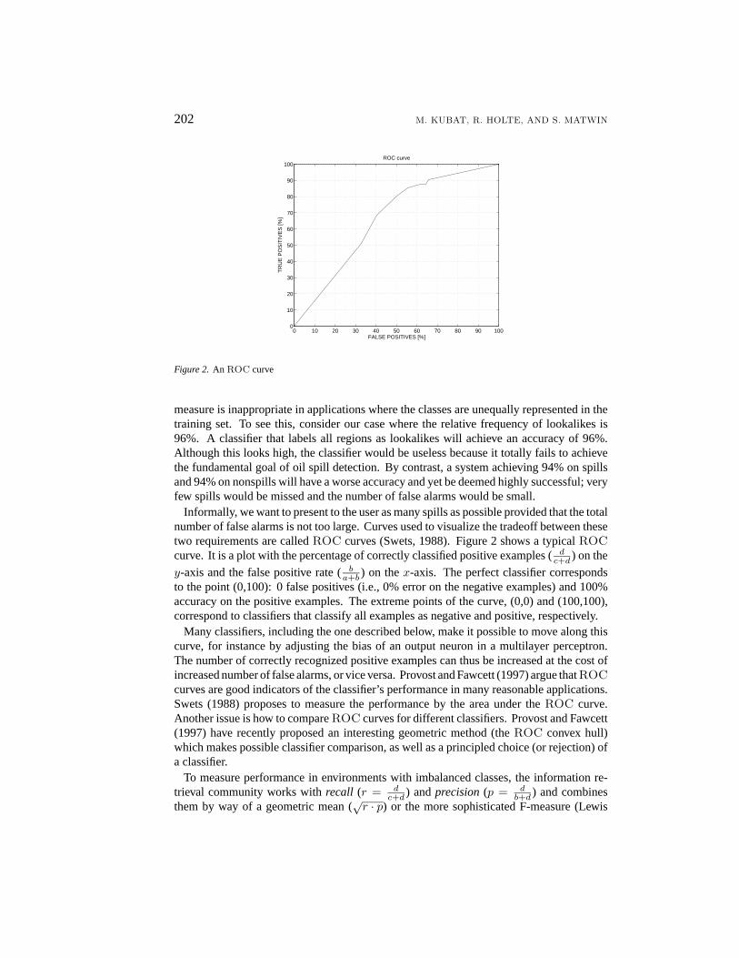
Figure 2. An ROC curve

measure is inappropriate in applications where the classes are unequally represented in thetraining set. To see this, consider our case where the relative frequency of lookalikes is96%. A classifier that labels all regions as lookalikes will achieve an accuracy of 96%.Although this looks high, the classifier would be useless because it totally fails to achievethe fundamental goal of oil spill detection. By contrast, a system achieving 94% on spillsand 94% on nonspills will have a worse accuracy and yet be deemed highly successful; veryfew spills would be missed and the number of false alarms would be small.

Informally, we want to present to the user as many spills as possible provided that the totalnumber of false alarms is not too large. Curves used to visualize the tradeoff between thesetwo requirements are calledROC curves (Swets, 1988). Figure 2 shows a typicalROC

curve. It is a plot with the percentage of correctly classified positive examples (dc+d ) on the

y-axis and the false positive rate (ba+b ) on thex-axis. The perfect classifier correspondsto the point (0,100): 0 false positives (i.e., 0% error on the negative examples) and 100%accuracy on the positive examples. The extreme points of the curve, (0,0) and (100,100),correspond to classifiers that classify all examples as negative and positive, respectively.

Many classifiers, including the one described below, make it possible to move along thiscurve, for instance by adjusting the bias of an output neuron in a multilayer perceptron.The number of correctly recognized positive examples can thus be increased at the cost ofincreased number of false alarms, or vice versa. Provost and Fawcett (1997) argue thatROC

curves are good indicators of the classifier’s performance in many reasonable applications.Swets (1988) proposes to measure the performance by the area under theROC curve.Another issue is how to compareROC curves for different classifiers. Provost and Fawcett(1997) have recently proposed an interesting geometric method (theROC convex hull)which makes possible classifier comparison, as well as a principled choice (or rejection) ofa classifier.

To measure performance in environments with imbalanced classes, the information re-trieval community works withrecall (r = d

c+d ) andprecision(p = db+d ) and combines

them by way of a geometric mean (√r · p) or the more sophisticated F-measure (Lewis


& Gale, 1994). Other measures have been suggested (van Rijsbergen, 1979, Chapter 7),including an information theoretic formula suggested by Kononenko and Bratko (1991).

The standard decision theoretic approach to defining the “optimal” tradeoff between falseand true positives is to assign relative costs to errors of omission and errors of commission,and to make the classification that minimizes expected cost (Pazzani et al., 1994). Onedeterrent to using this approach is that the costs are often hard to determine and may involvemultiple considerations whose units are incommensurable (e.g., monetary cost, pollutionlevels, international reputation). Decision analysis techniques have been developed to copewith this difficulty (von Winterfeldt & Edwards, 1986; Keeney & Raiffa, 1993). Butthese techniques, which involve the eliciting of subjective judgements from the end userby a trained decision analyst, are awkward to use with a system such as ours which isnot targeted at a particular end user. Moreover, MacDonald Dettwiler Associates requiredthe system to be readily customizable to each user; this precludes the labour intensiveknowledge elicitation techniques of decision analysis or knowledge based systems.

We decided that in the version of the system that will be delivered to end users therewill not be a preprogrammed way of condensing theROC curve to a single performancemeasure. Instead, the user will be able to move along the curve and choose the point thatbest meets his/her current needs. In this way, the user perceives the performance in termsof two parameters (the frequency of true positives and of false positives). This is typicalof fielded systems. As pointed out by Saitta, Giordana and Neri (1995), systems that serveas tools for users confronting a specific decision (e.g., whether to send an aircraft to verifya spill and document the incident) should not be constrained to use a scalar performancemeasure. The user needs to be able to tune the system’s behavior so as to trade off variousconflicting needs.

Although, in general, the challenge is to build a system that can produce classifiers acrossa maximally broad range of itsROC curve, in the course of development we did not haveaccess to the users that would tune the system to their particular circumstances. However,we needed a performance measure to provide immediate feedback (in terms of a singlevalue) on our design decisions. This measure would have to address the clear inadequacyof accuracy, which is unuseable in our problem. To this end, we have mainly used thegeometric mean (g −mean), g =

√acc+× acc−, whereacc+ = d

c+d is the accuracy onthe positive examples, andacc− = a

a+b , is the accuracy on the negative examples. Thismeasure has the distinctive property of being independent of the distribution of examplesbetween classes, and is thus robust in circumstances where this distribution might changewith time or be different in the training and testing sets. Another important and distinctiveproperty is thatg − mean is nonlinear. A change ofp percentage points inacc+ (oracc−) has a different effect ong − mean depending on the magnitude ofacc+: thesmaller the value ofacc+, the greater the change ofg − mean. This property meansthat the “cost” of misclassifying each positive example increases the more often positiveexamples are misclassified. A learning system based ong − mean is thereby forced toproduce hypotheses that correctly classify a non-negligible fraction of the positive trainingexamples. On the other hand,g − mean is less than ideal for filtering tasks, because itignores precision.


6. Methodological Issues

After the problem formulation and the choice of the performance measure, the designer ofa learning system must turn his or her attention to the specific idiosyncracies of the dataavailable for learning. In the oil spill detection problem we faced the following issues.

1. Examples come in small batches, each with different characteristics.

2. The data is sparse and the training set is imbalanced.

3. There is no guarantee that the examples available for the system development arerepresentative of the examples that will arise after deployment.

4. Feature engineering is required.

5. System development is done in a dynamically changing environment.

Let us look at these issues in turn. The first issue is how to learn and experiment withbatchedexamples. Table 2 gives some details about our data. The nine images (batches)contain a total of 41 positive examples and 896 negative examples, and the characteristics ofthe individual images can vary considerably. The images all come from the same satelliteand the same general geographical location (strait of Juan de Fuca between VancouverIsland and the northern tip of Washington state), but the times when they were obtained aredifferent. One can thus expect that the images contain oil spills of different origin and ofdifferent types.

One possible approach is to view the individual batches in the training set as coming froma different “context” and use a context sensitive learning algorithm as suggested by Turney(1993), Widmer and Kubat (1996), and Kubat and Widmer (1996). However, our initialexperiments with simple contextual normalization techniques were not entirely successful(partly because of the scarcity of the data), so we decided not to pursue context sensitivelearning. Moreover, we do not always know what the contextual parameters are. Evenwhen we know that in reality there is a contextual variable that influences the classifier (e.g.the wind speed), often we have no way to compute the value of this variable.

An alternative approach is to combine all the examples into one large dataset in the hopethat the learning algorithm will be able to detect systematic differences between batchesand react by creating a disjunctive definition with a disjunct, say, for each batch. However,if the individual batches have a relatively small number of positive examples such a systemwill be prone to the problem of small disjuncts (Holte, Acker & Porter, 1989). Moreover,the batches that have many examples (e.g., images 2 and 9) will dominate those that havefew (e.g., image 1).

Batched examples also raise an issue about experimental methodology. Suppose that allexamples are mixed in one data file from which a random subset is selected for training,leaving the rest for testing. This means that examples from the same batch can appear bothin the training and testing sets. As a result, the observed performance will be optimisticcompared to the deployed system’s actual performance on completely unseen batches. Thisphenomenon will be experimentally demonstrated below. There really is no valid alternativebut to separate the batches used for training from those for testing, as has been done by Burlet al. (1998), Cherkauer and Shavlik (1994), Ezawa et al. (1996), and Fawcett and Provost(1997). The particular testing method we use is “leave-one-batch-out” (LOBO), which is


Table 2.The numbers of positive and negative examples in the images

image 1 2 3 4 5 6 7 8 9 all

positives 8 4 2 6 2 4 3 5 7 41negatives 3 180 101 129 60 70 76 80 197 896total 11 184 103 135 62 74 79 85 204 937

the same as the traditional leave-one-out methodology except that one whole batch is leftout on each iteration rather than just one example.

Overfitting is a term normally applied to a learning algorithm that constructs a hypothesisthat “fits” the training data “too well.” Dietterich et al. (1997) use “overfitting” in a differentsense. They apply the term when an algorithm developer tunes a learning algorithm, orits parameter settings, to optimize its performance on all the available data. This type ofoverfitting, which we callovertuning, is a danger whenever all available data is used foralgorithm development/tuning. Like ordinary overfitting, overtuning can be detected, if notavoided, by using only part of the data for algorithm development and using the remainderof the data for final system testing, as was done by Lubinsky (1994). If data is not held outfor final system testing, the observed performance of the system cannot be confidently usedas an estimate of the expected performance of the deployed system. Unfortunately, we hadtoo little oil spill data to hold any out for final system testing in the development phase ofthe project. The system will be tested on fresh data in the field trials that are scheduled forwinter 1998.

Dietterich et al. (1997) circumvented their lack of data by modeling some key character-istics of the data and generating a large artificial dataset, an idea proposed by Aha (1992).The point is to use the synthetic data for system development, and to return to the real dataonly for final system testing. We were hampered in using this method by the fact that ourdata comes in small batches which were fairly dissimilar. We would have had to model boththe within-batch characteristics and the across-batch characteristics, and we simply did nothave enough data or batches to do this with any certainty. To try to ensure that our learningalgorithm is not specific to our particular dataset, we have tested it on other datasets havingsimilar characteristics (Kubat, Holte & Matwin, 1997).

Another issue is theimbalanceof the dataset’s class distribution. This issue has twofacets. The first, discussed above, is that when working with imbalanced datasets it isdesirable to use a performance measure other than accuracy. The second facet, shown byKubat et al. (1997) and by Kubat and Matwin (1997), is that learning systems designed tooptimize accuracy, such asC4.5 (Quinlan, 1993) and the 1-nearest-neighbor rule (1-NN),can behave poorly if the training set is highly imbalanced. The induced classifiers tendto be highly accurate on negative examples but usually misclassify many of the positives.This will be demonstrated in the experimental part of this paper.

Two approaches promise to solve this problem. The first attempts tobalancethe classes.One way to do this is to discard those examples that are considered harmful. As earlyas the late sixties, Hart (1968) presented a mechanism that removes redundant examplesand, somewhat later, Tomek (1976) introduced a simple method to detect borderline andnoisy examples. In machine learning the best known sampling technique is windowing


(Catlett, 1991). For more recent alternatives, see, for instance, Aha, Kibler and Albert(1991), Zhang (1992), Skalak (1994), Floyd and Warmuth (1995), and Lewis and Catlett(1994). Variations of data reduction techniques, namely those that remove only negativeexamples, are analyzed by Kubat and Matwin (1997). Conversely, the training set can bebalanced by duplicating the training examples of the minority class or by creating newexamples by corrupting existing ones with artificial noise (DeRouin et al., 1991). Solbergand Solberg (1996) do both; positives are duplicated and negatives are randomly sampled.Honda, Motizuki, Ho, and Okumura (1997) reduce the imbalance by doing classification intwo stages. In the first stage, the negatives most similar to the positives are included in thepositive class. The second stage distinguishes these negatives from the true positives. Thiscan be seen as a special case of multitask learning (Caruana, 1993), the more general ideabeing to define supplementary classification tasks in which the classes are more equallybalanced. Pazzani et al. (1994) assign different weights to examples of different classes,Fawcett and Provost (1997) prune the possibly overfit rule set learned from an imbalancedset, and Ezawa et al. (1996) force the learner to consider relationships between certainattributes above others.

The second approach is to develop an algorithm that isintrinsically insensitiveto the classdistribution in the training set. Extreme examples of this are algorithms that learn frompositive examples only. A less extreme approach is to learn from positive and negativeexamples but to learn only rules that predict the positive class, as is done byBRUTE

(Riddle et al., 1994). By measuring performance only of the positive predicting rules,BRUTE is not influenced by the invariably high accuracy on the negative examples thatare not covered by the positive predicting rules. OurSHRINK algorithm (Kubat et al.,1997) follows the same general principle—find the rule that best summarizes the positiveexamples—but uses a definition of “best” (g−mean) that takes into account performanceof the negative predicting rules as well as the positive predicting ones. In section 7, wedescribeSHRINK and demonstrate empirically that its performance does not change asimbalance grows.

The third methodological issue is thevalidity of the data selection.We deliberately ac-quired only images containing oil slicks so as to maximize the number of positive examplesin our dataset. However, this means that the distribution of examples in our dataset is dif-ferent from the distribution that will arise naturally when the system is fielded. Fortunately,in our domain, all the lookalikes are natural phenomena whose presence in an image isindependent of the presence of an oil slick. It is only because of this fact that we can haveconfidence that our performance on the acquired images will extend to “normal” images,which mostly will not contain slicks.

Another methodological issue isfeature engineering.We did not do any large scaleconstructive induction, as, for example, was done by Cherkauer and Shavlik (1994). Insteadwe relied on our domain experts to define useful features. The importance of good featureswas impressed upon them from the outset, and a significant fraction of their energy hasbeen invested in this direction. Some features are generic while others are motivated bytheoretical considerations and therefore implicitly represent domain knowledge. In thefinal feature set, a region is described by 49 features representing characteristics such asthe position of the region’s centroid point, the region’s shape, its area, its intensity, the


sharpness and jaggedness of its edges, its proximity to other regions, and information aboutthe background (the sea) in the image containing the region.

Our approach to feature construction has not been entirely successful. Many of thefeatures for which the experts had high expectations have not proven particularly helpfulfor classification. An open research issue is whether the domain knowledge used to definethese features could have been used to better advantage if it had been captured explicitlyand used to guide learning as suggested by Clark and Matwin (1993) or perhaps to guideconstructive induction as investigated by Ioerger, Rendell and Subramanian (1995).

The discriminating power of our features is significantly influenced by the parametersettings of the low-level image processing. Unfortunately, the settings that extract thegreatest number of oil spills do not optimize the features’ discriminating power, and wedecided it was most important to maximize the number of oil spills. If we had had moreimages, we would have been able to improve our learning algorithm’s performance bysetting the image processing parameters to optimize the features. On the positive side,machine learning provided valuable feedback to the experts about the direct impact of anew feature on the performance measure and about the role played by the feature in theinduced classifier. It was important that the feature’s contribution to a decision be consistentwith the experts’ expectations (Lee et al., 1998).

The final methodological issue relates to our working in a highly dynamic environment.The set of images and the set of features for each image changed throughout the project,as did the exact details of the low-level image processing. Each of these changes produceda new dataset. The learning algorithms, too, were under constant development, and theexperimental method changed several times before settling onLOBO. The constant fluxdemanded careful bookkeeping about the exact versions of the datasets, algorithms, andmethodology used in each experiment. This was done manually. A tool for this bookkeep-ing, for example an extension of the data preparation tool reported by Rieger (1995), wouldbe a valuable contribution to applications of this kind.

7. Experimental Results

In this section we present experimental studies of two of the central research issues thatarose in our application: (1) imbalanced training sets, and (2) batched examples.

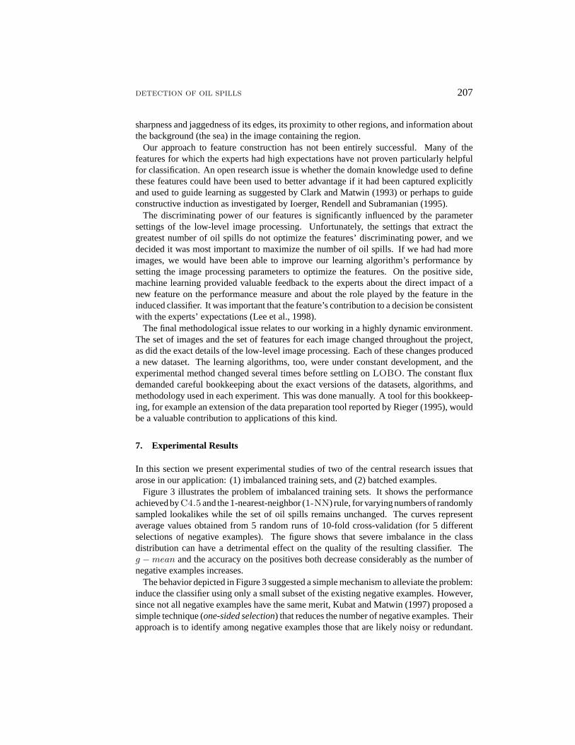
Figure 3 illustrates the problem of imbalanced training sets. It shows the performanceachieved byC4.5and the 1-nearest-neighbor (1-NN) rule, for varying numbers of randomlysampled lookalikes while the set of oil spills remains unchanged. The curves representaverage values obtained from 5 random runs of 10-fold cross-validation (for 5 differentselections of negative examples). The figure shows that severe imbalance in the classdistribution can have a detrimental effect on the quality of the resulting classifier. Theg −mean and the accuracy on the positives both decrease considerably as the number ofnegative examples increases.

The behavior depicted in Figure 3 suggested a simple mechanism to alleviate the problem:induce the classifier using only a small subset of the existing negative examples. However,since not all negative examples have the same merit, Kubat and Matwin (1997) proposed asimple technique (one-sided selection) that reduces the number of negative examples. Theirapproach is to identify among negative examples those that are likely noisy or redundant.


0 100 200 300 400 500 600 700 800 9000

10

20

30

40

50

60

70

80

90

100

number of negative examples

accu

racy

C4.5

0 100 200 300 400 500 600 700 800 9000

10

20

30

40

50

60

70

80

90

1001−NN

accu

racy


Figure 3.Performance ofC4.5 (left) and the 1-nearest-neighbor rule (right) achieved on the testing set for differentnumbers of randomly sampled negative examples. Solid:g −mean; dashed: accuracy on negative examples;dotted: accuracy on positive examples.

Table 3.Accuracies achieved withC4.5

and1-NN after one-sided selection

classifier g −mean acc+ acc-

C4.5 81.1 76.0 86.61-NN 67.2 54.0 83.4

A heuristic measure, introduced by Tomek (1976), is used to identify noisy examples,while the potentially redundant ones are determined using an approach adapted from Hart(1968). One-sided selection removes from the training set redundant and noisy negativeexamples. The results achieved using one-sided selection are summarized in Table 3. Theseresults were obtained using 5 random runs of 10-fold cross-validation starting with all theexamples; in each run, the training set was reduced using the one-sided selection beforetheC4.5 or 1-NN rule was applied.C4.5 clearly benefited from this data reduction, bothon the positive and on the negative examples (the improvement is statistically significantaccording to a t-test). However, in the case of the1-NN rule, one-sided selection producedno significant improvement.

One-sided selection is a method for altering an imbalanced training dataset so thataccuracy-based systems will perform reasonably well. An alternative approach is to de-velop an algorithm that is insensitive to imbalance. With this aim in mind, we developedtheSHRINK algorithm.

Three principles underlieSHRINK’s design. First, if positive examples are rare, do notsubdivide them when learning—dividing a small number of positive examples into two orthree groups would make reliable generalization over each group impossible. The secondprinciple is to induce a classifier of very low complexity. InSHRINK, the classifier isrepresented by anetwork of tests. The tests have the formxi ∈ [min ai,max ai] whereiindexes the attributes. Denote byhi the output of thei-th test, and lethi = 1 if the test


0 100 200 300 400 500 600 700 800 9000

10

20

30

40

50

60

70

80

90

100


accu

racy

SHRINK

Figure 4. SHRINK’s performance. Solid:g − mean; dashed: accuracy on negatives; dotted: accuracy onpositives.

suggests a positive label, andhi = −1 otherwise. The example is classified as positive if∑i hi · wi > θ, wherewi is the weight of thei-th test (see below). The thresholdθ gives

the user the opportunity to relax or tighten the weight of evidence that is necessary for aregion to be classified as an oil spill.

The third principle is to focus exclusively on regions of the instance space where positiveexamples occur. In the induction of the tests,SHRINK begins by establishing the “best”interval along each attribute, starting with the smallest interval containing all positive ex-amples, and on every iteration shrinking the interval by eliminating either the left or rightendpoint, whichever results in the betterg−mean score. For each attribute, this producesa set of nested intervals from which the one with the maximumg −mean is selected asthe test. Tests withg −mean g < 0.5 are then discarded. The weight,wi, of thei-th testis defined to bewi = log(gi/(1 − gi)), wheregi is theg − mean of the i-th test. Thisexpression assigns higher weights to tests with small errors. The fact that the system usesonly tests withgi > 0.5 ensures that all weights are positive.

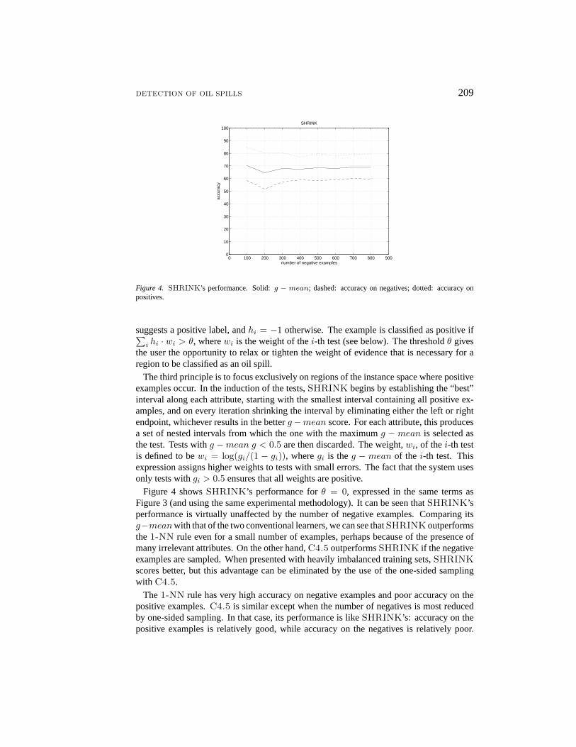
Figure 4 showsSHRINK’s performance forθ = 0, expressed in the same terms asFigure 3 (and using the same experimental methodology). It can be seen thatSHRINK’sperformance is virtually unaffected by the number of negative examples. Comparing itsg−meanwith that of the two conventional learners, we can see thatSHRINK outperformsthe1-NN rule even for a small number of examples, perhaps because of the presence ofmany irrelevant attributes. On the other hand,C4.5 outperformsSHRINK if the negativeexamples are sampled. When presented with heavily imbalanced training sets,SHRINK

scores better, but this advantage can be eliminated by the use of the one-sided samplingwith C4.5.

The1-NN rule has very high accuracy on negative examples and poor accuracy on thepositive examples.C4.5 is similar except when the number of negatives is most reducedby one-sided sampling. In that case, its performance is likeSHRINK’s: accuracy on thepositive examples is relatively good, while accuracy on the negatives is relatively poor.


0 10 20 30 40 50 60 70 80 90 1000

10

20

30

40

50

60

70

80

90

100ROC curve

FALSE POSITIVES [%]

TR

UE

PO

SIT

IVE

S [%

]

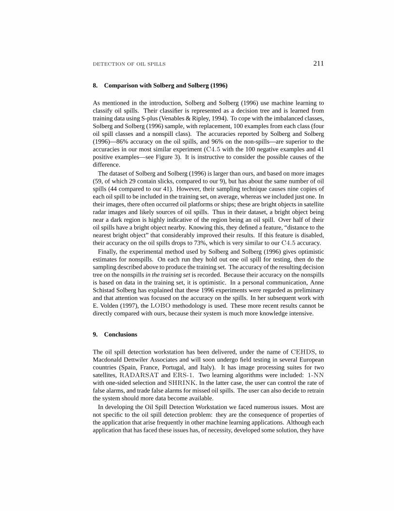
Figure 5. An exampleROC curve (testing set) obtained fromSHRINK on the oil spill data

Table 4.Leave-one-batch-out (LOBO)compared to conventionalcross-validation (CV)

g −mean acc+ acc-

CV 70.9 82.5 60.9LOBO 62.5 78.1 50.1

As mentioned earlier, it is important in our application to be able to explore the tradeoffbetween true and false positives dynamically. InSHRINK, the user can move along theROC curve by adjusting the thresholdθ. TheROC curve produced in this way is shownin Figure 5. The operator can thus reduce the frequency of false positives at the cost ofan increased number of false negatives. Note, however, that although the curve shown iscontinuous, there are actually only a discrete number of points on the curve that can beproduced by varyingθ.

One of the methodological issues mentioned in the previous sections is the requirementthat the classifier be trained on one set of batches (images) and tested on another set ofbatches. Table 4 illustrates this point using some results obtained from experimenting withSHRINK (θ = 0). The first row (CV) contains the results obtained using the 10-foldcross-validation (average from 5 random runs) applied to the dataset containing all theexamples from all images (so that examples from the same image can occur in both thetraining and the testing sets). These results are clearly superior to those in the second row,which are obtained using the leave-one-batch-out (LOBO) methodology. The experimentshows that the images differ systematically, and therefore they cannot be safely combinedinto one large dataset.


8. Comparison with Solberg and Solberg (1996)

As mentioned in the introduction, Solberg and Solberg (1996) use machine learning toclassify oil spills. Their classifier is represented as a decision tree and is learned fromtraining data using S-plus (Venables & Ripley, 1994). To cope with the imbalanced classes,Solberg and Solberg (1996) sample, with replacement, 100 examples from each class (fouroil spill classes and a nonspill class). The accuracies reported by Solberg and Solberg(1996)—86% accuracy on the oil spills, and 96% on the non-spills—are superior to theaccuracies in our most similar experiment (C4.5 with the 100 negative examples and 41positive examples—see Figure 3). It is instructive to consider the possible causes of thedifference.

The dataset of Solberg and Solberg (1996) is larger than ours, and based on more images(59, of which 29 contain slicks, compared to our 9), but has about the same number of oilspills (44 compared to our 41). However, their sampling technique causes nine copies ofeach oil spill to be included in the training set, on average, whereas we included just one. Intheir images, there often occurred oil platforms or ships; these are bright objects in satelliteradar images and likely sources of oil spills. Thus in their dataset, a bright object beingnear a dark region is highly indicative of the region being an oil spill. Over half of theiroil spills have a bright object nearby. Knowing this, they defined a feature, “distance to thenearest bright object” that considerably improved their results. If this feature is disabled,their accuracy on the oil spills drops to 73%, which is very similar to ourC4.5 accuracy.

Finally, the experimental method used by Solberg and Solberg (1996) gives optimisticestimates for nonspills. On each run they hold out one oil spill for testing, then do thesampling described above to produce the training set. The accuracy of the resulting decisiontree on the nonspillsin the training setis recorded. Because their accuracy on the nonspillsis based on data in the training set, it is optimistic. In a personal communication, AnneSchistad Solberg has explained that these 1996 experiments were regarded as preliminaryand that attention was focused on the accuracy on the spills. In her subsequent work withE. Volden (1997), theLOBO methodology is used. These more recent results cannot bedirectly compared with ours, because their system is much more knowledge intensive.

9. Conclusions

The oil spill detection workstation has been delivered, under the name ofCEHDS, toMacdonald Dettwiler Associates and will soon undergo field testing in several Europeancountries (Spain, France, Portugal, and Italy). It has image processing suites for twosatellites,RADARSAT andERS-1. Two learning algorithms were included:1-NN

with one-sided selection andSHRINK. In the latter case, the user can control the rate offalse alarms, and trade false alarms for missed oil spills. The user can also decide to retrainthe system should more data become available.

In developing the Oil Spill Detection Workstation we faced numerous issues. Most arenot specific to the oil spill detection problem: they are the consequence of properties ofthe application that arise frequently in other machine learning applications. Although eachapplication that has faced these issues has, of necessity, developed some solution, they have


not yet been the subject of thorough scientific investigation. They are open research issuesof great importance to the applications community.

Perhaps the most important issue is that of imbalanced classes. It arises very often inapplications and considerably reduces the performance of standard techniques. Numerousmethods for coping with imbalanced classes have been proposed, but they are scatteredthroughout the literature. At the very least, a large scale comparative study is needed toassess the relative merits of these methods and how they work in combination. Manyindividual methods, theSHRINK algorithm for example, can undoubtedly be improvedby further research. It seems important to study small imbalanced training sets separatelyfrom large ones. In the latter, positive examples are numerous even though they are greatlyoutnumbered by negative examples. Some of the published methods for learning from im-balanced classes, require numerous examples of the minority class. The Bayesian approachdescribed by Ezawa et al. (1996), for example, works with several thousand examples inthe minority class, while we were limited to fewer than fifty.

Learning from batched examples is another issue which requires further research. Withthe resources (manpower, data) available in this project, we were not able to devise a learningalgorithm that could successfully take advantage of the grouping of the training examplesinto batches. However, we believe further research could yield such an algorithm. Learningfrom batched examples is related to the issues of learning in the presence of context, as thebatches often represent the unknown context in which the training examples were collected.Learning in context has only recently been recognized as an important problem re-occurringin applications of machine learning (Kubat & Widmer, 1996).

Various tradeoffs arose in our project which certainly warrant scientific study. In for-mulating a problem, one must choose the granularity of the examples (images, regions,or pixels in our application) and the number of classes. Different choices usually lead todifferent results. For instance, having several classes instead of just two reduces the numberof training examples per class but also provides additional information to the induction pro-cess. How can one determine the optimal choice? Another tradeoff that arose was betweenthe discriminating power of the features and the number of examples.

In machine learning applications, there is no standard measure of performance. Classi-fication accuracy may be useful in some applications, but it is certainly not ideal for all.The research challenge is to develop learning systems that can be easily adapted to differentperformance measures. For example, cost sensitive learning algorithms work with a param-eterizedfamily of performance measures. Before running the learning algorithm, the userselects a specific measure within this family by supplying values for the parameters (i.e., thecosts). A second example is the “wrapper approach” to feature selection (Kohavi & John,to appear), parameter setting (Kohavi & John, 1995), or inductive bias selection (Provost& Buchanan, 1995). It can be adapted easily to work with any performance measure. Ourapproach was to have the learning system generate hypotheses across the full range of theROC curve and permit the user to interactively select among them.

Feature engineering is a topic greatly in need of research. Practitioners always emphasizethe importance of having good features, but there are few guidelines on how to acquirethem. Constructive induction techniques can be applied when there is sufficient data thatovertuning will not occur. An alternative to purely automatic techniques are elicitationtechniques such as structured induction (Shapiro, 1987). More generally, one can elicit


domain knowledge, as Solberg and Volden (1997) have done, and use a learning algorithmguided by a weak domain theory as done by Clark and Matwin (1993).

Our experience in this project highlights the fruitful interactions that are possible betweenmachine learning applications and research. The application greatly benefited from—indeed would not have succeeded without—many ideas developed in the research commu-nity. Conversely, the application opened new, fertile research directions. Future researchin these directions will directly benefit the next generation of applications.

Acknowledgments

The research was sponsored by PRECARN, Inc. The research of the second and third authorsis sponsored by the Natural Sciences and Engineering Research Council of Canada and byCommunications and Information Technology Ontario. Thanks are due to Mike Robson,the principal contributor to the image processing subsystem, for his active cooperation withus and for providing invaluable comments on the development of the machine learningsubsystem. We also thank Peter Turney (National Research Council of Canada, Ottawa) forhis advice on all aspects of this work, and Anne Schistad Solberg (Norwegian ComputingCenter, Oslo) for the information she provided about her work. The authors appreciatecomments of the anonymous referees and the insightful feedback from Ron Kohavi andFoster Provost.

References

Aha, D., Kibler, D., & Albert, M. (1991). Instance-Based Learning Algorithms.Machine Learning, 6(1), 37–66.Aha, D. (1992). Generalizing from Case Studies: A Case Study.Proceedings of the Ninth International Conference

on Machine Learning(pp. 1–10), Morgan Kaufmann.Brodley, C., & Smyth, P. (1995). The Process of Applying Machine Learning Algorithms.Working Notes

for Applying Machine Learning in Practice: A Workshop at the Twelfth International Conference on MachineLearning, Technical Report AIC-95-023 (pp. 7–13), NRL, Navy Center for Applied Research in AI, Washington,DC.

Burl, M.C., Asker, L., Smyth, P., Fayyad, U.M., Perona, P., Crumpler, L., & Aubele, J. (this issue). Learning toRecognize Volcanoes on Venus.Machine Learning, 30, 165–194.

Caruana, R. (1993). Multitask Learning: A Knowledge-based Source of Inductive Bias.Proceedings of the TenthInternational Conference on Machine Learning(pp. 41–48), Morgan Kaufmann.

Catlett, J. (1991). Megainduction: A Test Flight.Proceedings of the Eighth International Workshop on MachineLearning(pp. 596–599), Morgan Kaufmann.

Cherkauer, K.J., & Shavlik, J.W. (1994). Selecting Salient Features for Machine Learning from Large CandidatePools through Parallel Decision-Tree Construction. In Kitano, H. & Hendler, J. (Eds.),Massively ParallelArtificial Intelligence(pp. 102-136), AAAI Press/MIT Press.

Clark, P. & Matwin, S. (1993). Using Qualitative Models to Guide Inductive Learning.Proceedings of the TenthInternational Conference on Machine Learning(pp. 49–56), Morgan Kaufmann.

Clearwater, S., & Stern, E. (1991). A Rule-Learning Program in High Energy Physics Event Classification.Comp.Physics Comm., 67, 159–182.

DeRouin, E., Brown, J., Beck, H., Fausett, L., & Schneider, M. (1991). Neural Network Training on UnequallyRepresented Classes. In Dagli, C.H., Kumara, S.R.T., & Shin, Y.C. (Eds.),Intelligent Engineering SystemsThrough Artificial Neural Networks, pp. 135–145, ASME Press.

Dietterich, T.G., Hild, H., & Bakiri, G. (1995). A Comparison of ID3 and Backpropagation for English Text-to-Speech Mapping.Machine Learning, 18, 51–80.

Dietterich, T.G., Lathrop, R.H., & Lozano-Perez, T. (1997). Solving the Multiple-Instance Problem with Axis-Parallel Rectangles.Artificial Intelligence, 89(1–2), 31–71.


Ezawa, K.J., Singh, M., & Norton, S.W. (1996). Learning Goal Oriented Bayesian Networks for Telecommu-nications Management.Proceedings of the Thirteenth International Conference on Machine Learning(pp.139–147), Morgan Kaufmann.

Fawcett, T., & Provost, F. (1997). Adaptive Fraud Detection.Data Mining and Knowledge Discovery, 1(3),291–316.

Fayyad, U.M., Weir, N., & Djorgovski, S. (1993).SKICAT: A Machine Learning System for AutomatedCataloging of Large Scale Sky Surveys.Proceedings of the Tenth International Conference on Machine Learning(pp. 112–119), Morgan Kaufmann.

Floyd, S., & Warmuth, M. (1995). Sample Compression, Learnability, and the Vapnik-Chervonenkis Dimension.Machine Learning, 21, 269–304.

Hart, P.E. (1968). The Condensed Nearest Neighbor Rule.IEEE Transactions on Information Theory, IT-14,515–516.

Haverkamp, D., Tsatsoulis, C., & Gogineni, S. (1994). The Combination of Algorithmic and Heuristic Methodsfor the Classification of Sea Ice Imagery.Remote Sensing Reviews, 9, 135–159.

Heerman, P. D., & Khazenie, N. (1992). Classification of Multispectral Remote Sensing Data using a back-propagation Neural Network.IEEE Trans. of Geoscience and Remote Sensing, 30, 81–88.

Holte, R. C., Acker, L., & Porter, B. W. (1989). Concept Learning and the Problem of Small Disjuncts.Proceedingsof the International Joint Conference on Artificial Intelligence(pp. 813–818), Morgan Kaufmann.

Honda, T., Motizuki, H., Ho, T.B., & Okumura, M. (1997). Generating Decision Trees from an Unbalanced DataSet. In van Someren, M., & Widmer, G. (Eds.),Poster papers presented at the 9th European Conference onMachine Learning(pp. 68-77).

Hovland, H. A., Johannessen, J. A., & Digranes, G. (1994). Slick Detection in SAT Images.Proceedings ofIGARSS’94(pp. 2038–2040).

Ioerger, T.R., Rendell, L.A., & Subramaniam, S. (1995). Searching for Representations to Improve ProteinSequence Fold-Class Prediction.Machine Learning, 21, 151–176.

Keeney, R.L., & Raiffa, H. (1993).Decisions with Multiple Objectives: Preferences and Value Tradeoffs, Cam-bridge University Press.

Kohavi, R., & John, G.H. (to appear). Wrappers for Feature Subset Selection.Artificial Intelligence(special issueon relevance).

Kohavi, R., & John, G.H. (1995). Automatic Parameter Selection by Minimizing Estimated Error.Proceedingsof the Twelfth International Conference on Machine Learning(pp. 304-312), Morgan Kaufmann.

Kononenko, I., & Bratko, I. (1991). Information-Based Evaluation Criterion for Classifier’s Performance.MachineLearning, 6, 67–80.

Kubat, M., Holte, R., & Matwin, S. (1997). Learning when Negative Examples Abound.Machine Learning:ECML-97, Lecture Notes in Artificial Intelligence 1224(pp. 146–153), Springer.

Kubat, M., & Matwin, S. (1997). Addressing the Curse of Imbalanced Training Sets: One-Sided Sampling.Pro-ceedings of the Fourteenth International Conference on Machine Learning(pp. 179–186), Morgan Kaufmann.

Kubat, M., Pfurtscheller, G., & Flotzinger D. (1994). AI-Based Approach to Automatic Sleep Classification.Biological Cybernetics, 79, 443–448.

Kubat, M., & Widmer, G. (Eds.) (1996).Proceedings of the ICML’96 Pre-Conference Workshop on Learning inContext-Sensitive Domains.

Langley, P., & Simon, H.A. (1995). Applications of Machine Learning and Rule Induction.Communications ofthe ACM, 38(11), 55–64.

Lee, Y., Buchanan, B.G., & Aronis, J.M. (this issue). Learning Rules to Predict Rodent Carcinogenicity.MachineLearning, 30, 217–240.

Lewis, D., & Catlett, J. (1994). Heterogeneous Uncertainty Sampling for Supervised Learning.Proceedings ofthe Eleventh International Conference on Machine Learning(pp. 148–156), Morgan Kaufmann.

Lewis, D., & Gale, W. (1994). A Sequential Algorithm for Training Text Classifiers.Proceedings of the Sev-enteenth Annual International ACM SIGIR Conference on Research and Development in Information Retrieval(pp. 3–12), Springer-Verlag.

Lubinsky, David (1994).Bivariate Splits and Consistent Split Criteria in Dichotomous Classification Trees. Ph.D.thesis, Computer Science, Rutgers University.

Murphy, P., & Aha, D. (1994). UCI Repository of Machine Learning Databases (machine-readable data repository).University of California, Irvine.

Ossen, A., Zamzow, T., Oswald, H., & Fleck, E. (1994). Segmentation of Medical Images Using Neural-NetworkClassifiers.Proceedings of the International Conference on Neural Networks and Expert Systems in Medicineand Healthcare (NNESMED’94)(pp. 427–432).


Pazzani, M., Merz, C., Murphy, P., Ali, K., Hume, T., & Brunk, C. (1994). Reducing Misclassification Costs.Proceedings of the Eleventh International Conference on Machine Learning(pp. 217–225), Morgan Kaufmann.

Pfurtscheller, G., Flotzinger, D., & Kalcher, J. (1992). Brain-Computer Interface - A New Communication Devicefor Handicapped Persons. In Zagler, W. (Ed.),Computer for Handicapped Persons: Proceedings of the ThirdInternational Conference(pp. 409–415).

Provost, F.J., & Buchanan, B.G. (1995). Inductive Policy: The Pragmatics of Bias Selection.Machine Learning,20(1/2), 35–62.

Provost, F.J., & Fawcett, T. (1997). Analysis and Visualization of Classifier Performance: Comparison underImprecise Class and Cost Distributions.Proceedings of the Third International Conference on KnowledgeDiscovery and Data Mining(pp. 43–48).

Quinlan, J.R. (1993).C4.5: Programs for Machine Learning.Morgan Kaufmann.Riddle, P., Segal, R., & Etzioni, O. (1994). Representation Design and Brute-Force Induction in a Boeing

Manufacturing Domain.Applied Artificial Intelligence, 8, 125–147.Rieger, A. (1995). Data Preparation for Inductive Learning in Robotics.Proceedings of the IJCAI-95 workshop

on Data Engineering for Inductive Learning(pp. 70–78).Saitta, L., Giordana, A., & Neri, F. (1995). What Is the “Real World”?.Working Notes for Applying Machine

Learning in Practice: A Workshop at the Twelfth International Conference on Machine Learning, TechnicalReport AIC-95-023 (pp. 34–40), NRL, Navy Center for Applied Research in AI, Washington, DC.

Shapiro, A.D. (1987).Structured Induction in Expert Systems. Addison-Wesley.Skalak, D. (1994). Prototype and Feature Selection by Sampling and Random Mutation Hill Climbing Algorithms.

Proceedings of the Eleventh International Conference on Machine Learning(pp. 293–301), Morgan Kaufmann.Solberg, A.H.S., & Solberg, R. (1996). A Large-Scale Evaluation of Features for Automatic Detection of Oil

Spills inERS SAR Images.IEEE Symp. Geosc. Rem. Sens (IGARSS)(pp. 1484–1486).Solberg, A.H.S., & Volden, E. (1997). Incorporation of Prior Knowledge in Automatic Classification of Oil Spills

in ERS SAR Images.IEEE Symp. Geosc. Rem. Sens (IGARSS)(pp. 157–159).Swets, J.A. (1988). Measuring the Accuracy of Diagnostic Systems.Science, 240, 1285–1293.Tomek, I. (1976). Two Modifications of CNN.IEEE Transactions on Systems, Man and Cybernetics, SMC-6,

769–772.Turney, P. (1995). Data Engineering for the Analysis of Semiconductor Manufacturing Data.Proceedings of the

IJCAI-95 workshop on Data Engineering for Inductive Learning(pp. 50–59).Turney, P. (1993). Exploiting Context when Learning to Classify.Proceedings of the European Conference on

Machine Learning(pp. 402–407), Springer-Verlag.van Rijsbergen, C.J. (1979).Information Retrieval (second edition), Butterworths.Venables, W.N., & Ripley, B.D. (1994).Modern Applied Statistics with S-Plus. Springer-Verlag.von Winterfeldt, D., & Edwards, W. (1986).Decision Analysis and Behavioral Research. Cambridge University

Press.Widmer, G., & Kubat, M. (1996). Learning in the Presence of Concept Drift and Hidden Contexts.Machine

Learning, 23, 69–101.Zhang, J. (1992). Selecting Typical Instances in Instance-Based Learning.Proceedings of the Ninth International

Machine Learning Workshop(pp. 470–479), Morgan Kaufmann.

Received March 4, 1997Accepted September 18, 1997Final Manuscript November 15, 1997

Date post:	19-Aug-2018
Category:	Documents
Upload:	truongnga
View:	217 times
Download:	0 times

Machine Learning for the Detection of Oil Spills in ...1007452223027.pdf · Machine Learning for...

Documents