HAL Id: tel-00150756 https://tel.archives-ouvertes.fr/tel-00150756 Submitted on 31 May 2007 HAL is a multi-disciplinary open access archive for the deposit and dissemination of sci- entific research documents, whether they are pub- lished or not. The documents may come from teaching and research institutions in France or abroad, or from public or private research centers. L’archive ouverte pluridisciplinaire HAL, est destinée au dépôt et à la diffusion de documents scientifiques de niveau recherche, publiés ou non, émanant des établissements d’enseignement et de recherche français ou étrangers, des laboratoires publics ou privés. Machine Observation of the Direction of Human Visual Focus of Attention Nicolas Gourier To cite this version: Nicolas Gourier. Machine Observation of the Direction of Human Visual Focus of Attention. Human- Computer Interaction [cs.HC]. Institut National Polytechnique de Grenoble - INPG, 2006. English. <tel-00150756>
Transcript
HAL Id: tel-00150756https://tel.archives-ouvertes.fr/tel-00150756
Submitted on 31 May 2007
HAL is a multi-disciplinary open accessarchive for the deposit and dissemination of sci-entific research documents, whether they are pub-lished or not. The documents may come fromteaching and research institutions in France orabroad, or from public or private research centers.
L’archive ouverte pluridisciplinaire HAL, estdestinée au dépôt et à la diffusion de documentsscientifiques de niveau recherche, publiés ou non,émanant des établissements d’enseignement et derecherche français ou étrangers, des laboratoirespublics ou privés.
Machine Observation of the Direction of Human VisualFocus of Attention
Nicolas Gourier
To cite this version:Nicolas Gourier. Machine Observation of the Direction of Human Visual Focus of Attention. Human-Computer Interaction [cs.HC]. Institut National Polytechnique de Grenoble - INPG, 2006. English.<tel-00150756>
DOCTEUR DE L’INSTITUT NATIONAL POLYTECHNIQUE DE GRENOBLE
Spécialité : Imagerie, Vision et RobotiqueEcole Doctorale : Mathématiques, Sciences et Technologie de l’Information
présentée et soutenue publiquementpar
Nicolas GOURIER
le 19 octobre 2006
MACHINE OBSERVATION OF THE DIRECTIONOF HUMAN VISUAL FOCUS OF ATTENTION
Directeur de thèse : M. James L. CROWLEY
JURY
Mme Catherine GARBAY , PrésidenteM. Roberto CIPOLLA, RapporteurMme Monique THONNAT, RapporteuseM. James L. CROWLEY, DirecteurMlle Daniela HALL , CodirectriceM. Josep R. CASAS, Examinateur
Thèse préparée dans le laboratoire GRAVIR – IMAG au sein du projet PRIMAINRIA Rhône-Alpes, 655 av. de l’Europe, 38334 Saint-Ismier, France.
2
3
Abstract
People often look at objects and people with which they are likely to interact. The firststep for computer systems to adapt to the user and to improve interaction and with people is tolocate where they are, and especially the location of their faces on the image. The next step isto track their focus of attention. For this reason, we are interested in techniques for estimatingand tracking gaze of people, and in particular the head pose.
This thesis proposes a fully automatic approach for head pose estimation independant of theperson identity using low resolution images acquired in unconstrained imaging conditions. Thedeveloped method is demonstrated and evaluated using a densly sampled face image database.We propose a new coarse-to-fine approach that uses both global and local appearance to estimatehead orientation. This method is fast, easy to implement, robust to partial occlusion, uses noheuristiques and can be adapted to other deformable objects. Face region images are normalizedin size and slant by a robust face tracker. The resulting normalized imagettes are projected ontoa linear auto-associative memory learned using the Widrow-Hoff rule. Linear auto-associativememories require very few parameters and offer the advantage that no cells in hidden layershave to be defined and class prototypes can be saved and recovered for all kinds of applications.A coarse estimation of the head orientation on known and unknown subjects is obtained bysearching the best prototype which matches the current image.
We search for salient facial features relevant for each headpose. Feature points are locallydescribed by Gaussian receptive fields normalized at intrinsic scale. These descriptors haveinteresting properties and are less expensive than Gabor wavelets. Salient facial regions foundby Gaussian receptive fields motivate the construction of a model graph for each pose. Eachnode of the graph can be displaced localy according to its saliency in the image. Linear auto-associative memories deliver a coarse estimation of the pose. We search among the coarse poseneighbors the model graph which obtains the best match. The pose associated with its salientgrid graph is selected as the head pose of the person on the image. This method does not useany heuristics, manual annotation or prior knowledge on theface and can be adapted to estimatethe pose of configuration of other deformable objects.
Keywords: Head pose estimation, focus of attention, real-time face tracking, linear auto-associative memory, Gaussian derivative receptive fields,feature saliency, grid graphs.
4
5
Résumé
Les personnes dirigent souvent leur attention vers les objets avec lesquels ils interagissent.Une première étape que doivent franchir les systèmes informatiques pour s’adapter aux utilisa-teurs et améliorer leurs interactions avec eux est de localiser leur emplacement, et en particulierla position de leur tête dans l’image. L’étape suivante est de suivre leur foyer d’attention. C’estpourquoi nous nous intéressons aux techniques permettant d’estimer et de suivre le regard desutilisateurs, et en particulier l’orientation de leur tête.
Cette thèse présente une approche complètement automatique et indépendante de l’identitéde la personne pour estimer la pose d’un visage à partir d’images basse résolution sous condi-tions non contraintes. La méthode developpée ici est évaluée et validée avec une base de don-nées d’images échantillonnée. Nous proposons une nouvelleapproche à 2 niveaux qui utilise lesapparences globales et locales pour estimer l’orientationde la tête. Cette méthode est simple,facile à implémenter et robuste à l’occlusion partielle. Les images de visage sont normaliséesen taille dans des images de faible résolution à l’aide d’un algorithme de suivi de visage. Cesimagettes sont ensuite projetées dans des mémoires autoassociatives et entraînées par la rè-gle d’apprentissage de Widrow-Hoff. Les mémoires autoassociatives ne nécessitent que peu deparamètres et évitent l’usage de couches cachées, ce qui permet la sauvegarde et le charge-ment de prototypes de poses du visage humain. Nous obtenons une première estimation del’orientation de la tête sur des sujets connus et inconnus.
Nous cherchons ensuite dans l’image les traits faciaux saillants du visage pertinents pourchaque pose. Ces traits sont décrits par des champs réceptifs gaussiens normalisés à l’échelleintrinsèque. Ces descripteurs ont des propriétés intéressantes et sont moins coûteux que lesondelettes de Gabor. Les traits saillants du visage détectés par les champs réceptifs gaussiensmotivent la construction d’un modèle de graphe pour chaque pose. Chaque nœud du graphe peutêtre déplacé localement en fonction de la saillance du pointfacial qu’il représente. Nous recher-chons parmi les poses voisines de celle trouvée par les mémoires autoassociatives le graphe quicorrespond le mieux à l’image de test. La pose correspondante est sélectionnée comme la posedu visage de la personne sur l’image. Cette méthode n’utilise pas d’heuristique, d’annotationmanuelle ou de connaissances préalables sur le visage et peut être adaptée pour estimer la posed’autres objets déformables.
Mots clés : estimation de l’orientation de la tête, foyer d’attention,suivi du visage en tempsréel, mémoires linéaires autoassociatives, champs réceptifs de dérivées gaussiennes, régionssaillantes, graphes.
6
Acknowledgements
I would like to thank all people who contributed in all manners to the achievement of mythesis work.
First of all, my thanks go to my supervisor Prof. James L. Crowley for his well adviseddiscussions and his motivation. I also would like to thank Dr. Daniela Hall for her ideas and herpatience. I am grateful to Roberto Cipolla, Monique Thonnat, Catherine Garbay and Josep R.Casas for their interest in my work and for being members of myjury.
I would like to thank Jérôme Maisonnasse for his criticism and for being a fun officemate,Olivier Riff who introduced me to the PRIMA group, Alban Caparossi for his collaboration,Augustin Lux for his help and open discussions, and Matthieuand Marina for sharing the office.Thanks to all PRIMA members, Patrick, Dominique, Alba, Stan, Matthieu, Julien, Rémi, Hai,Suphot, Olivier, Sonia, Oliver and Caroline for the cool atmosphere in the group. It was apleasure to work at the INRIA Rhône-Alpes in Grenoble.
My special thanks go to Véronique and Guillaume for their special collaboration, Jean-Baptiste for his jokes and to all my friends of the ML for theirsupport.
I would also like to thank all people who posed for the database and all people who partici-pated to the experiment.
Finally, I would like to thank my parents and my grandmother for their unconditional sup-port and love.
7
8
Contents
I Résumé français 13
1 Introduction 151.1 Estimation de la pose de la tête par apparences globale etlocale . . . . . . . . 161.2 Contributions principales de cette thèse . . . . . . . . . . . .. . . . . . . . . 17
2 Contenu de la thèse 212.1 Approches pour estimer l’orientation de la tête . . . . . . .. . . . . . . . . . . 212.2 Capacités humaines à estimer l’orientation de la tête . .. . . . . . . . . . . . . 24
Observation de la direction du foyer visueld’attention par ordinateur
-Résumé français
13
Chapitre 1
Introduction
La plupart des ordinateurs modernes sont autistes. Peu de nouvelles technologies existentpour recenser les interactions sociales entre des personnes et entre une personne et une machine.En conséquence, les systèmes artificiels distraient souvent les utilisateurs avec des actions in-appropriées et n’ont pas ou peu de capacités à utiliser les interactions humaines pour corrigerleur comportement.
Un aspect important des interactions sociales est la capacité à observer l’attention humaine.Généralement, les personnes localisent le foyer d’attention des personnes en observant leursvisages et leurs regards. En majeure partie, l’intérêt et l’attention d’une personne peuvent êtreestimés à partir de l’orientation de sa tête.
Dans cette thèse, nous nous intéressons au problème de l’estimation de l’orientation, oupose, de la tête sur des images non contraintes. La pose de la tête est déterminée par troisangles : l’inclinaison par rapport au corps (slant), l’inclinaison horizontale (pan) et l’inclinaisonverticale (tilt). L’angle slant varie autour de l’axe longitudinal. L’angle tilt varie autour de l’axelatéral, quand une personne regarde de bas en haut. Cet angleest le plus difficile à estimer.L’angle pan varie autour de l’axe vertical, quand une personne tourne sa tête de gauche à droite.Notre objectif est d’estimer ces trois angles, ce qui servira de première base à l’estimation del’attention.
Beaucoup de techniques d’estimation de regard et de pose de la tête présentes dans lalittérature utilisent des équipements spécifiques, comme l’illumination infrarouge, l’électro-oculographie, les casques portables ou des lentilles de contact spécifiques [59, 167, 33]. Dessystèmes utilisant des caméras actives ou la vision stéréo sont disponibles dans le commerce[162, 96, 120]. Bien que de telles techniques soient très précises, elles sont généralement chèreset trop intrusives pour beaucoup d’applications. Les systèmes basés sur la vision par ordinateurprésentent un choix plus accessible et moins intrusif.
Notre but est de proposer une méthode non intrusive et qui ne nécessite pas d’équipementspécifique pour estimer l’orientation de la tête. En particulier, nous nous intéressons aux tech-nologies robustes au changement d’identité sous des conditions d’images non contraintes. Leshumains peuvent estimer grossièrement la pose d’un objet à partir d’une image. En outre, l’es-
15
16 CHAPITRE 1. INTRODUCTION
timation de l’orientation de la tête à partir d’une image estla base pour une estimation plusprécise à partir de plusieurs images.
Les approches pour estimer l’orientation de la tête à partird’une simple image peuventêtre regroupées en 4 familles : les approches géométriques 2D, les approches géométriques3D, les approches par transformation faciale et les approches par classifieurs. Les approchesgéométriques 2D utilisent certains traits du visage pour trouver des correspondances et estimerainsi l’orientation. Ces méthodes sont précises mais nécessitent une bonne résolution de l’imagedu visage et voient leurs performances se dégrader sur des mouvements de tête amples. Lesapproches géométriques 3D appliquent un modèle 3D de la têtesur l’image pour retrouverla pose. Ces techniques sont encore plus précises, mais requièrent plus de temps de calcul,une bonne résolution ainsi qu’une forte connaissance préalable du visage. Les approches partransformation faciale utilisent certaines propriétés faciales pour obtenir une estimation de lapose de la tête. De telles méthodes sont simples à mettre en œuvre, mais sont parfois instableset non robustes à l’identité. Les approches par classifieursrésolvent le problème en cherchantla meilleure correspondance avec l’image courante et un modèle préalablement appris. Cesméthodes sont très rapides, mais ne peuvent délivrer qu’uneestimation grossière et l’utilisateurn’a pas de retour d’information si le système échoue. Nous développons une approche hybrideglobale et locale à 2 niveaux pour estimer l’orientation de la tête dont les performances sontcomparables aux performances humaines.
1.1 Estimation de la pose de la tête par apparences globale etlocale
Dans cette thèse, nous proposons une approche complètementautomatique d’estimationde pose de la tête indépendante de l’identité sur des images prises dans des conditions noncontraintes. Cette approche combine les avantages des approches globales qui utilisent l’appa-rence entière de l’image du visage pour la classification et les approches locales qui utilisentles informations contenues dans les voisinages de pixels etleurs relations dans l’image, sansutiliser d’heuristique ni de connaissance préalable sur levisage. Nous présentons un systèmed’estimation de l’orientation de la tête à 2 niveaux basé surles mémoires autoassociatives li-néaires et les graphes de champs réceptifs gaussiens. Notreméthode marche sur des images nonalignées comme dans les conditions réelles et sa performance est comparable aux performanceshumaines.
Pour mesurer efficacement la performance d’un algorithme d’estimation de pose de la tête,il est nécessaire de le tester sur une base de données représentative. Dans la littérature, lesméthodes différentes sont souvent testées sur des bases de données différentes, ce qui rend lescomparaisons difficiles. Une base de données représentative doit contenir un nombre suffisantd’orientations pour observer le comportement de l’algorithme sur chaque pose. Cette mêmebase de données doit être symétrique et suffisamment échantillonnée. Si une méthode marche
1.2. CONTRIBUTIONS PRINCIPALES DE CETTE THÈSE 17
bien sur la plupart des angles, elle peut être adaptée au suivi de pose de la tête en temps réel eten conditions réelles, dans lesquelles l’orientation de latête n’est pas discrète mais continue.
Dans nos expériences, nous utilisons la Pointing 2004 Head Pose Image Database [39], unebase de données échantillonnée de 15 en 15 degrés couvrant une demi-sphère d’orientations,soit des angles pan et tilt variant de -90 à +90 degrés. Cette base contient 15 sujets. Pour chaquesujet, il y a 2 séries de 93 images de pose. L’apprentissage etle test peuvent être faits soit surles sujets connus en effectuant une validation croisée sur les séries, soit sur les sujets inconnusen effectuant un algorithme Jack-Knife sur les sujets.
Les capacités humaines pour estimer l’orientation de la tête sont largement inconnues. Nousne savons pas si les humains ont une aptitude naturelle à estimer la pose de la tête à partir d’unesimple image ou s’ils doivent être entraînés à cette tâche à partir d’images d’exemple. De plus,nous ne connaissons pas l’exactitude avec laquelle une personne peut estimer les angles pan ettilt. Dans ses études, Kersten [65] montre que les poses faceet profil sont utilisées comme desposes clés par le cerveau humain. Comme référence, nous avons évalué les performances d’ungroupe de personnes à l’estimation de l’orientation de la tête sur une partie de la Pointing’04Head Pose Image Database. Ces expériences montrent que notre algorithme obtient des résultatssimilaires à ceux obtenus par le groupe de personnes.
Dans notre méthode, une première estimation de la pose est obtenue en cherchant la meil-leure mémoire autoassociative linéaire correspondant à l’image du visage. Nous combinonscette estimation avec une autre méthode basée sur les régions saillantes du visage pertinentespoour chaque pose. Les régions saillantes sont décrites localement par des champs réceptifsgaussiens normalisés à leurs échelles intrinsèques, données par le premier maximum local dulaplacien normalisé. Ces descripteurs ont des propriétés intéressantes et sont moins coûteux àcalculer que les ondelettes de Gabor. Les régions saillantes détectées de cette façon permettentla construction d’un modèle de graphe pour chaque pose. Chaque nœud du graphe peut êtredéplacé localement en fonction de sa saillance et est annotépar une densité de probabilité devecteurs de champs réceptifs gaussiens normalisés et clusterisés hiérarchiquement, pour repré-senter les différents aspects que peuvent avoir un même trait du visage selon différentes iden-tités. Les mémoires autoassociatives linéaires donnent une première estimation de la pose. Cerésultat est raffiné en cherchant parmi les poses voisines lemeilleur modèle de graphe corres-pondant. La pose associée au modèle de graphe est sélectionnée comme la pose du visage de lapersonne.
1.2 Contributions principales de cette thèse
Nos expériences montrent que les humains réussissent à bienreconnaître les poses faceet profil, mais moins les poses intermédiaires. Le groupe de personnes a effectué une erreurmoyenne de11.85o en pan et11.04o en tilt. L’erreur minimale se trouve pour la pose 0 degré,ce qui correspond à la vue de face. L’angle pan semble plus naturel à estimer. Ces résultatssuggèrent que le système visuel humain utilise face et profilcomme des poses clés, comme
18 CHAPITRE 1. INTRODUCTION
stipulé dans [65].Dans notre méthode, la région de l’image correspondant au visage est normalisée dans
une image de petite résolution en utilisant un système de suivi de visage. Les mémoires auto-associatives linéaires sont utilisées pour apprendre des prototypes d’orientations de la tête. Cesmémoires sont simples à construire, ne requièrent que peu deparamètres et sont adaptées pourl’estimation de la pose du visage sur des sujets connus et inconnus. Les prototypes peuvent êtreappris en utilisant un ou deux axes. Avec une erreur moyenne de moins de10o en pan et en tiltpour des sujets connus, notre méthode est plus performante que les réseaux de neurones [152],l’Analyse par Composantes Principales et les modèles de tenseurs [145]. Nous obtenons uneerreur moyenne de10o en pan et16o en tilt sur des sujets inconnus. Apprendre les angles panet tilt ensemble n’améliore pas significativement les résulats. Nous apprenons donc ces anglesséparément, ce qui réduit le nombre de prototypes à utiliser. Ces résultats sont obtenus sur desimages non alignées. Les prototypes de poses du visage peuvent être sauvegardés et chargésultérieurement pour d’autres applications. Notre algorithme de première estimation de la posefonctionne à 15 images par seconde, ce qui est suffisant pour des applications vidéo telles queles interactions homme-machine, la vidéosurveillance et les environnements intelligents.
Cette première estimation est raffinée en décrivant les images du visage par des champsréceptifs gaussiens normalisés à leurs échelles intrinsèques. Les dérivées gaussiennes décriventl’apparence de voisinages de pixels et présentent un moyen efficace pour détecter les traits duvisage indépendamment de leur taille et de leur illumination. De plus, elles ont des propriétésd’invariance intéressantes. Les images de visage sont ainsi décrites par des vecteurs de faibledimension. Les régions saillantes du visage sont découvertes en analysant les régions qui par-tagent une apparence similaire sur un rayon limité. Nous trouvons que les principaux traitssaillants du visage sont : les yeux, le nez, la bouche et le contour du visage. Ces résultats res-semblent aux traits faciaux regardés par les humains selon les études de Yarbus [165].
Les graphes de champs réceptifs gaussiens améliorent l’estimation de la pose obtenue enpremière estimation. La structure de graphe décrit à la foisl’apparence des voisinages de pixelset leurs relations géométriques dans l’image. Les résultats sont meilleurs en effectuant un clus-tering hiérarchique en chaque nœud du graphe. Les graphes recouvrant la totalité de l’imagedu visage sont plus performants que ceux ne recouvrant qu’une partie du visage. Plus grandeest la portion d’image recouverte, plus importantes sont les relations géométriques. De plus,paramétrer le déplacement local maximal d’un nœud en fonction de sa saillance résulte en unemeilleure estimation que fixer un même déplacement local pour chaque nœud. Un nœud placésur un trait saillant du visage représente un point pertinent pour la pose considérée et ne doit pastrop se déplacer de son emplacement initial. Au contraire, un nœud placé dans une région peusaillante ne représente pas de point pertinent pour la pose et peut bouger. En utilisant cette mé-thode, nous obtenons un système d’estimation de la pose de latête avec une exactitude de10o
en pan et12o en tilt sur des sujets inconnus. Cet algorithme ne requiert pas d’heuristique, d’an-notation manuelle ou de connaissance préalable sur le visage et peut être adapté pour estimerl’orientation ou la configuration d’autres objets déformables.
L’estimation de pose du visage est testée sur des séquences vidéo de la IST CHIL Pointing
1.2. CONTRIBUTIONS PRINCIPALES DE CETTE THÈSE 19
Database. Le contexte temporel offre un gain en temps de calcul considérable. La pose duvisage sur l’image suivante se trouve dans le voisinage de lapose courante. Nous avons obtenuune erreur moyenne de22.5o en pan. Les sujets sont différents de ceux de la base de donnéesPointing’04. L’estimation de l’orientation de la tête peutégalement servir d’entrée pour dessystèmes attentionnels [85].
20 CHAPITRE 1. INTRODUCTION
Chapitre 2
Contenu de la thèse
L’attention visuelle contribue plus que l’attention auditive dans l’attention humaine [129].De plus, plusieurs études rapportent que le regard fournit des informations importantes sur lefoyer d’attention [130, 75]. La direction du regard est déterminée par l’orientation de la tête etla position de la pupille sur l’œil. Durant un regard rapide,il n’y a presque pas de rotation de latête. Les yeux peuvent mouvoir leur orbite à une vitesse allant jusqu’à 500 degrés par seconde.Cependant, pour un regard soutenu, les muscles des yeux ont besoin d’effort pour se maintenirdésaxés. La rotation de la tête soulage alors cet effort. C’est pourquoi la plupart des étudesmontrent que l’orientation contribue généralement plus que la position de la pupille sur l’œilà l’attention visuelle. Dans ses études, Stiefelhagen [138, 130] a trouvé que les gens tournentla tête plus souvent que les yeux dans 69 % des cas et la direction de la tête est la même quecelle des yeux dans 89 % en situation de meeting. En outre, détecter les pupilles sur une imagerequiert une haute résolution de l’image du visage, et les yeux peuvent cligner, ce qui les rendplus difficiles à détecter. C’est pourquoi nous nous intéressons à l’estimation de l’orientation dela tête.
2.1 Approches pour estimer l’orientation de la tête
Le but de cette étude est de déterminer l’orientation, ou pose, de la tête sur des imagesnon contraintes. La pose de la tête est déterminée par trois angles : l’inclinaison par rapportau corps (slant), l’inclinaison horizontale (pan) et l’inclinaison verticale (tilt). Ces trois anglessont illustrés sur la figure 2.1. L’angle slant varie autour de l’axe longitudinal. L’angle tilt varieautour de l’axe latéral, quand une personne regarde de bas enhaut. Cet angle est le plus difficileà estimer. L’angle pan varie autour de l’axe vertical, quandune personne tourne sa tête de gaucheà droite. Ces trois angles recouvrent complètement les mouvements de la tête.
Beaucoup de techniques d’estimation de regard et de pose de la tête présentes dans lalittérature utilisent des équipements spécifiques, comme l’illumination infrarouge, l’électro-oculographie, les casques portables ou des lentilles de contact spécifiques [59, 167, 33]. Des
21
22 CHAPITRE 2. CONTENU DE LA THÈSE
FIG. 2.1 – Les trois angles de rotation de la tête [25].
systèmes utilisant des caméras actives ou la vision stéréo sont disponibles dans le commerce[162, 96, 120]. Bien que de telles techniques soient très précises, elles sont généralement chèreset trop intrusives pour beaucoup d’applications. Les systèmes basés sur la Vision par Prdinateurprésentent un choix plus accessible et moins intrusif. Les humains peuvent fournir une estima-tion de la pose à partir d’une simple image. De plus, une bonneestimation de la pose du visagepeut améliorer l’estimation de la pose à partir de plusieursimages.
L’estimation de l’orientation de la tête possède beaucoup d’applications dans des domainesvariés, mais est un problème difficile et se heurte à certainsobstacles. Contrairement à la plupartdes problèmes en Vision par Ordinateur, il n’y a pas de cadre de travail unifié pour cette tâche.Presque tous les auteurs traitant du sujet utilisent leur propre cadre de travail et leurs propresmétriques. Le premier aspect important pour un système d’estimation de la pose du visage estla résolution minimale à laquelle il peut fonctionner. Certains algorithmes ne peuvent marcherqu’à haute résolution (500x500 pixels), tandis que d’autres peuvent fonctionner avec des imagesde très petite résolution (32x32 pixels). Ceci nous mène à unautre aspect du problème, les me-sures de performance. Il n’y a pas de métriques communes pourla tâche d’estimation de la pose.De plus, la façon dont la précision ou l’erreur moyenne sont calculées n’est pas toujours expli-cite dans la littérature. De même, la séparation entre les images utilisées pour l’apprentissage etle test n’est pas toujours claire. L’estimation de l’orientation de la tête diffère de l’estimation del’orientation d’un objet en ce que la tête est déformable et change avec l’identité de la personne.Les variations de couleur de peau, des cheveux, des joues et des autres caractéristiques facialesrendent l’estimation de la pose du visage difficilement robuste aux changements d’identité. Ceproblème est simplifié quand le système est conçu pour un utilisateur particulier. Cette remarquenous mène au dernier aspect important du problème : le choix de la base de données. Une basede données fiable pour l’estimation de la pose devrait couvrir un certain nombre d’angles et êtrebien échantillonnée pour permettre de voir le comportementd’un algorithme sur les différentesposes. Si un système fonctionne correctement pour la plupart des angles, il peut être adapté poursuivre le mouvement de la tête sur des séquences vidéo. Enfin,quand une base de données estemployée, nous devons savoir quelles parties sont utilisées pour l’apprentissage et pour le test.
Les approches pour estimer l’orientation de la tête à partird’une simple image peuventêtre regroupées en 4 familles : les approches géométriques 2D, les approches géométriques3D, les approches par transformation faciale et les approches par classifieurs. Les approches
2.1. APPROCHES POUR ESTIMER L’ORIENTATION DE LA TÊTE 23
géométriques 2D utilisent certains points du visage pour trouver des correspondances et estimerainsi l’orientation. Les points du visage de référence sontsouvent les yeux [133, 163, 134, 8,16, 36, 37]. Si ces derniers peuvent fournir une estimation de l’angle horizontal pan, ils nesont pas suffisants pour estimer l’angle vertical tilt. C’est pourquoi les auteurs utilisent souventd’autres points comme la bouche [169, 58, 126, 26, 47, 155], les sourcils [103], le nez [48, 17]ou même les trous du nez [142, 143, 4]. Un modèle plus complet utilisant 6 points faciaux aété proposé par Gee & Cipolla [31, 32]. Utiliser plus de points permet d’obtenir une estimationde la pose plus fiable, mais la position de ces points sur le visage peut changer d’une personneà une autre et certains peuvent ne pas être détectés sous des angles de tête trop grands. Cesméthodes sont précises mais nécessitent une bonne résolution de l’image du visage, dépendentde l’algorithme de détection de caractéristiques facialeset voient leurs performances se dégradersur des mouvements de tête amples.
Les approches géométriques 3D appliquent un modèle 3D de la tête sur l’image pour re-trouver la pose. La première technique de correspondance a été proposée par Huttenlocher [55],et améliorée ensuite par Azarbayejani et al. [2] pour suivrele mouvement des objets. Sa per-formance a augmenté avec l’utilisation de l’algorithme EM avec moindres carrés [15], le fluxoptique [88] ou l’utilisation de texture [111]. Cependant,le modèle 3D de visage est souventrigide, alors que le visage humain est déformable et varié. Une méthode permettant d’apprendreun modèle de visage en ligne a été proposée par Vachetti [147]. Les approches géométriques3D sont très précises, mais requièrent beaucoup de temps de calcul, une bonne résolution del’image ainsi qu’une forte connaissance préalable du visage pour fonctionner correctement.
Les approches par transformation faciale utilisent certaines propriétés faciales pour obtenirune estimation de la pose de la tête. Ces approches sont génériques et nécessitent peu de calculs.Certains auteurs utilisent la position des cheveux par rapport au visage [14, 154, 121], la dissi-militude entre les deux yeux [18, 22] ou encore l’assymétrieentre les parties gauche et droitedu visage [50, 95, 25] pour estimer l’orientation de la tête.Bien que simples à mettre en œuvre,de telles méthodes sont parfois instables et non robustes aux changements d’identité.
Les approches par classifieurs résolvent le problème en cherchant la meilleure correspon-dance avec l’image courante et un modèle préalablement appris. Une méthode populaire declassification est l’Analyse par Composantes Principales (ACP) proposée par Turk & Pent-land [146]. Elle a été utilisée pour l’estimation de la pose de tête par McKenna & Gong[106, 34, 92, 91, 35, 122]. Néanmoins, les images d’entraînement utilisées sont souvent alignéesmanuellement et l’ACP a tendance à être sensible à l’alignement et aux changements d’identité.D’autres méthodes utilisent des espaces propres d’ondelettes de Gabor [157, 98, 97], des KernelACP [77], des modèles de tenseurs, des LEA [145], des KDA [13], des SVM [52, 102, 156], desLGBP [84] ou des réseaux de neurones [116, 136, 132, 130, 135,152, 131]. Ces méthodes nenécessitent pas de connaissances préalables sur le visage,mais ont parfois un nombre importantde paramètres à régler, et le nombre de dimensions à utiliserou de cellules dans les couches ca-chées est déterminé manuellement. Ces méthodes sont rapides, mais ne peuvent délivrer qu’uneestimation grossière et l’utilisateur n’a pas de retour d’information si le système échoue.
Nous voyons que les approches pour estimer l’orientation dela tête peuvent généralement
TAB. 2.1 –Comparaison entre approches locales et globales.
se diviser en deux catégories : les approches locales qui utilisent l’information contenue dansles voisinages de pixels et les approches globales qui utilisent l’image entière du visage. Lesavantages et les inconvénients de ces deux types d’approchesont resumés dans le tableau 2.1.Augmenter la résolution de l’image du visage à traiter peut permettre une combinaison de mé-thodes globales et locales. À notre connaissance, peu de travaux mêlant les deux types d’ap-proche ont été effectués. Wu & Trivedi [160] ont récemment proposé un système permettantd’obtenir une estimation de la pose avec des KDA, puis de la raffiner en utilisant des graphesélastiques. Cependant, l’utilisation de ces graphes nécessitent d’annoter les points faciaux surtoutes les images. De plus, nous ne savons pas si le choix de chaque point est pertinent pourl’estimation de la pose. Nous proposons une méthode d’estimation de l’orientation de la tête uti-lisant une approche hybride globale et locale ne nécessitant pas de connaissances préalables surle visage ni d’annotation manuelle. Nous décrivons cette approche dans les sections suivantes,mais d’abord nous devons établir quelles sont les capacitéshumaines pour estimer la pose duvisage.
2.2 Capacités humaines à estimer l’orientation de la tête
Le but de cette section est de déterminer l’exactitude qui peut être attendue d’un systèmed’orientation de la tête fiable pour des applications dans des environnements intelligents. Leshumains estiment généralement le focus visuel d’attentionsur des images à partir de l’orienta-tion de la tête. Cependant, leurs capacités demeurent en majeure partie inconnues. Nous avonsdemandé à un groupe de personnes d’estimer la pose du visage sur des images. Nous avonsensuite mesuré leurs performances avec différentes métriques. Un résultat important de cetteexpérience est que les humains sont plus aptes à estimer l’orientation horizontale que l’orienta-tion verticale.
2.2. CAPACITÉS HUMAINES À ESTIMER L’ORIENTATION DE LA TÊTE 25
2.2.1 Travaux apparentés
La base psychophysique des aptitudes humaines à estimer l’orientation de la tête demeure enmajeure partie inconnue. Nous ne savons pas si les humains ont une capacité naturelle à estimerles angles de la tête ou s’ils acquièrent cette capacité avecl’expérience. À notre connaissance,il y a peu de données disponibles permettant de mesurer les compétences humaines pour cettetâche. Selon Kersten [65], les poses face et profil sont utilisées comme poses clés par le cerveauhumain et sont les mieux reconnues. L’image 2.2 présente un exemple de compétition phéno-ménale de poses ; les poses face et profil sont activées inconsciemment par notre cerveau, maispas les autres. Nous ne connaissons pas la performance humaine sur les poses intermédiaires etverticales.
FIG. 2.2 – Projection cylindrique aplatie d’un visage humain [65]. Toutes les poses horizontalessont présentes sur cette image, mais notre cerveau a tendance à ne distinguer que les poses faceet profil.
2.2.2 Protocole expérimental
Notre objectif est d’évaluer les performances des humains sur l’estimation de l’orienta-tion de la tête aux angles pan et tilt, pour les comparer ensuite avec celles obtenues par notresystème. Pour rendre possible cette comparaison, les deux performances doivent être évaluéessur la même base de données. Nous avons choisi d’utiliser desimages de la base de don-nées Pointing 2004 Head Pose Image Database [39]. Cette basede données est échantillon-née tous les 15 degrés en pan, tous les 15/30 degrés en tilt et couvre une demi-sphère deposes allant de -90 à +90 degrés sur les 2 axes. L’angle pan peut donc prendre les valeurs(0,±15,±30,±45,±60,±75,±90), où les valeurs négatives correspondent aux poses droiteset les valeurs positives correspondent aux poses gauches. L’angle tilt peut prendre les valeurs(−90,−60,−30,−15, 0, +15, +30, +60, +90), où les valeurs négatives correspondent aux po-ses basses et les valeurs positives correspondent aux poseshautes. De plus amples détails surcette base de données se trouvent dans l’annexe A.
26 CHAPITRE 2. CONTENU DE LA THÈSE
Un autre but de notre expérience est de découvrir si un axe estplus pertinent qu’un autrepour les humains. Pour ce faire, nous devons être en mesure dedire si l’estimation de l’anglepan ou de l’angle tilt est naturelle ou non. Si un angle se révèle être plus naturel à estimer, celasignifie que l’axe sur lequel il évolue est plus pertinent pour les humains dans leur vie de tousles jours.
Nous avons mesuré la performance d’un groupe de 72 sujets surl’estimation de l’orientationde la tête. Dans notre expérience, les sujets étaient répartis en 36 hommes et 36 femmes, âgésde 15 à 80 ans. On demande au sujet d’examiner une image de visage et d’entourer la réponsecorrespondant à son estimation de la pose. L’expérience estdivisée en 2 parties effectuées dansun ordre aléatoire : une pour l’estimation de l’angle pan, une pour l’estimation de l’angle tilt. 65images pour l’angle pan et 45 images pour l’angle tilt issuesde la Pointing’04 Head Pose ImageDatabase sont présentées au sujet pendant une durée de 7 secondes dans un ordre aléatoire,différent pour chaque sujet. Présenter les images selon un ordre aléatoire différent à chaque foisnous permet de mesurer les performances des sujets sur l’estimation de la pose du visage defaçon non biaisée sur des images indépendantes, et non sur une séquence d’images prédéfinie.La durée de présentation de 7 secondes est suffisamment longue pour permettre au sujet dechercher sa réponse et suffisamment courte pour obtenir une réponse immédiate de sa part. Il ya 5 images pour chaque angle. Durant l’expérience d’estimation de l’angle pan, des symboles"+" et "-" sont indiqués à côté de l’image, comme le montrent les images de la figure 2.3, pourque le sujet ne confonde pas les poses gauches et droites.
FIG. 2.3 – Exemples d’images de test présentées au sujet pendantl’expérience.
Un autre objectif important de cette expérience est d’obtenir les meilleures performances hu-maines sur l’estimation de la pose de la tête, pour les comparer ensuite avec les résultats obtenuspar notre système. Cependant, nous ne savons pas si cette tâche est naturelle pour les humains.C’est pourquoi les sujets furent divisés aléatoirement en 2sous-groupes : les sujets "Calibrés"et les sujets "Non Calibrés". Les sujets calibrés ont pu inspecter des images d’exemple étique-tées en orientation aussi longtemps qu’ils le souhaitaientavant de commencer l’expérience. Desexemples d’images d’entraînement sont presentés sur la figure 2.4. Les sujets non calibrés n’ontvu aucune image d’entraînement avant de commencer. Avoir créé ces deux sous-groupes aléa-toirement permet de voir si un entraînement préalable augmente les performances des sujets sur
2.2. CAPACITÉS HUMAINES À ESTIMER L’ORIENTATION DE LA TÊTE 27
l’estimation de l’orientation de la tête.
FIG. 2.4 – Exemples d’images d’entraînement montrées aux sujets "Calibrés" pour l’angle pan.
À la fin de notre expérience, nous présentons au sujet une image issue des travaux de Kersten[65]. Cette image est montrée sur la figure 2.2 et représente la projection cylindrique aplatie d’unvisage humain sur l’axe pan. Tous les angles pan sont visibles sur cette image. Nous demandonsau sujet d’entourer les angles qu’il voit sur l’image. Le butde cette question est de confirmerl’utilisation des poses face et profil comme poses clés par lecerveau humain
2.2.3 Résultats et discussion
Pour mesurer les performances humaines, nous devons définirdes métriques. La métriqueprincipale est l’erreur moyenne en pan et en tilt. Cette mesure est définie par la moyenne desdifférences absolues entre la pose théoriquep(k) et la posep∗(k) estimée par le sujet (2.1) pourl’image k. N est le nombre total d’images sur chaque axe. Nous calculons également l’erreurmaximale sur chaque axe pour chaque sujet (2.2). Une autre mesure intéressante est le taux declassification correcte, défini par le nombre de bonnes réponses sur le nombre total de réponses(2.3). Comme l’échantillon d’images de la base de données utilisée contient le même nombred’images pour chaque pose, nous pouvons calculer une autre métrique : l’erreur moyenne parpose (2.4). Cette métrique permet de voir les poses qui sont bien reconnues par les sujets.
ErreurMoyenne =1
N·
N∑
k=1
‖p(k) − p∗(k)‖ (2.1)
ErreurMax = maxk‖p(k) − p∗(k)‖ (2.2)
ClassificationCorrecte =Card{ImagesClassifiees}
Card{Images} (2.3)
ErreurMoyenne(P ) =1
Card{Images ∈ P} ·∑
k∈P
‖p(k) − p∗(k)‖ (2.4)
Nous avons calculé ces métriques pour tous les sujets et tousles sous-groupes. Les résultatssur les axes pan et tilt sont presentés dans les tableaux 2.2 et 2.3. L’erreur moyenne est de
28 CHAPITRE 2. CONTENU DE LA THÈSE
11.9 degrés en pan et 11 degrés en tilt. L’erreur maximale varie entre 30 et 60 degrés, ce quiest supérieur au pas d’échantillonnage de 15 degrés. Ceci prouve que la base de données estsuffisamment échantillonnée pour les sujets.
Pour mettre en relief des différences significatives de performances entre les groupes, nousavons effectué un test d’hypothèse en utilisant un test de Student-Fisher avec un seuil de con-fiance de 95 %. Les détails de cette opération se trouvent en Annexe B. Les sujets calibrés nesont pas significativement meilleurs que les sujets non calibrés pour l’estimation de l’angle pan.Par contre, la différence est significative pour l’angle tilt. Les sujets calibrés sont significati-vement meilleurs que les sujets non calibrés pour l’estimation de cet angle. Ce résultat montreque l’estimation de l’angle pan semble être naturelle, contrairement à celle de l’angle tilt. Cecipeut être dû au fait que les gens tournent plus souvent la têtede gauche à droite que de hauten bas pendant les interactions sociales [135, 64, 128]. Leshumains font plus attention auxchangements d’orientation de tête sur l’axe horizontal.
L’erreur moyenne par pose en pan et en tilt est montrée sur la figure 2.5. Les sujets recon-naissent bien les poses face et profil, mais moins bien les poses intermédiaires. La pose la mieuxreconnue est la pose frontale. Ce fait est confirmé par la présentation de l’image cylindrique devisage de Kersten à la fin de l’expérience. 81% des sujets n’ont pas vu de poses autres que faceet profil sur cette image. Ces résultats montrent que les poses face et profil sont utilisées par lesystème visuel humain comme des poses clés, comme suggéré dans [65].
FIG. 2.5 – Erreur moyenne par pose en pan et en tilt de différents groupes.
2.3 Suivi robuste de visage
Cette section décrit le système de suivi de visage temps réelutilisé dans la thèse. Cet al-gorithme, présenté en détail dans [37], est utilisé pour la détection des visages dans la base dedonnées Pointing 2004, bien que toute autre détection robuste, comme Ada-Boost [151], puisseêtre utilisée pour cette étape. Nous recherchons d’abord les régions de l’image correspondant auvisage à l’aide d’un histogramme de chrominance de peau. Le calcul de la chrominance(r, g)d’un pixel (x, y) est effectué en normalisant les composantes rouge et verte du vecteur de cou-leur (R, G, B) par son intensité lumineuseR + G + B. La densité de probabilité conditionnelledes vecteurs de chrominance(r, g) d’appartenir à une region de peau peut être estimée en utili-
30 CHAPITRE 2. CONTENU DE LA THÈSE
sant un histogramme. La règle de Bayes nous donne une relation directe entre un pixel(x, y) etsa probabilitép((x, y) ∈ Peau|r, g) d’être placé dans une région de peau. En effectuant le quo-tient des histogrammes de l’image entière et de peau, nous obtenons une meilleure répartitionde cette probabilité en fonction des autres objets présentssur l’image. Nous obtenons ainsi unecarte de probabilité sur toute l’image :
Pour suivre le visage dans une image, celui-ci doit se retrouver isolé. Sa position, sa tailleet son orientation sont estimées et suivies à l’aide d’un filtre de Kalman d’ordre 0 [61]. Leprocessus de tracking prédit une région d’intérêt (RDI) dans laquelle doit se trouver le visage etqui sera multipliée par une fenêtre gaussienne. Cette opération permet de focaliser la rechercheuniquement sur le visage suivi et d’accélérer le temps de calcul. Dans la RDI seront calculésles premier et second moments de la carte de probabilité ainsi obtenue. Ces moments délimitentune ellipse sur l’image correpondant à la région du visage. Cette région est appelée visageestimé. Un exemple de suivi de visage est illustré sur la figure 2.6. La différence entre le visageestimé à l’image courante et le visage estimé à l’image précédente permet de calculer le visageprédit à l’image suivante et la nouvelle RDI. Cette étape estappelée prédiction-vérification.À l’initialisation, le visage prédit peut être égal soit à une sélection manuelle de l’utilisateur,soit à l’image entière. Pour détecter le visage sur les images ne contenant qu’un seul visage, lesystème est lancé sans intervention de l’utilisateur sur l’image entière jusqu’à ce que le visageestimé se soit stabilisé, ce qui est généralement le cas après 10 itérations. Le système de suivide visage fonctionne en temps-réel sur des images de 384x288pixels sur Pentium 800 MHz.
FIG. 2.6 – De gauche à droite : RDI d’un visage dans l’image, Calcul de la carte de probabilitéavec fenêtre gaussienne dans la RDI, Ellipse délimitant le visage dans l’image.
À partir des premier et second moments du visage estimé, nouspouvons normaliser l’imagedu visage en taille et en inclinaison dans une imagette de plus petite résolution en niveauxde gris. La normalisation offre plusieurs avantages. Tout d’abord, elle permet aux opérations
2.4. ESTIMATION DE LA POSE DE LA TÊTE PAR APPARENCE GLOBALE 31
suivantes d’être indépendantes de la taille et de l’inclinaison de l’image d’origine. Les temps decalcul ne dépendent alors plus que de la taille de l’imagette. De plus, cette opération permet dene conserver que les changements d’intensité lumineuse. Undernier avantage important est derendre tous les visages droits, et ainsi de pouvoir localiser les mêmes points faciaux à peu prèsdans les mêmes régions pour chaque pose. Dans nos expériences, les imagettes ont une taille de23x30 pixels. Un exemple de normalisation d’une image de visage est montré sur la figure 2.7.Toutes les opérations ultérieures ont lieu dans cette imagette. La normalisation de la région duvisage est une étape utile à notre système d’estimation de pose de la tête.
FIG. 2.7 – Détection et normalisation de la région de l’image correspondant au visage.
2.4 Estimation de la pose de la tête par apparence globale
Dans cette section, nous utilisons les imagettes normalisées du visage obtenues par le sys-tème de suivi robuste pour apprendre des prototypes d’orientations de la tête. Les imagettesreprésentant la même pose sont injectées dans une mémoire autoassociative, entraînée par larègle d’apprentissage de Widrow-Hoff. La classification des poses se fait en comparant l’imagedu visage d’origine et les images reconstruites par les prototypes. La pose dont l’image recons-truite est la plus similaire à l’image source est sélectionnée comme pose courante.
2.4.1 Mémoires autoassociatives linéaires
Les mémoires autoassociatives linéaires sont un cas particulier de réseaux de neurones àune couche où les entrées sont associées à elles-mêmes en sortie. Elles ont été utilisées pour lapremière fois par Kohonen pour sauvegarder et charger des images [70]. Ces objets associentdes images à leur classe respective, même si les images sont dégradées ou une partie en estcachée. Une imagex′ en niveaux de gris est décrite par son vecteur normaliséx = x′
‖x′‖. Un
ensemble deM images composées deN pixels d’une même classe est sauvegardé dans lamatriceX = (x1, x2, ..., xM) de tailleN x M . La mémoire autoassociative de la classek estreprésentée par la matrice de connexionWk, de tailleN x N . Le nombre de cellules dans lamatrice est égal au nombre de pixels de l’image au carré. Son calcul a donc une complexité deO(N2). La réponse d’une cellule est égale à la somme de ses entrées multipliées par les poids dela matrice. L’image reconstruiteyk est donc obtenue en calculant le produit de l’image sourcex
par la matrice de connexionWk :
32 CHAPITRE 2. CONTENU DE LA THÈSE
yk = Wk · x (2.5)
La similarité de l’image source et d’une classe d’imagesk est estimée comme le cosinus deleurs vecteursx etyk :
cos(x, y) = yT .x =y′T .x′
‖y′T‖‖x′‖ (2.6)
Comme les vecteursx et y sont normalisés en énergie, leur cosinus est compris entre 0et 1, oùun score de 1 représente une correspondance parfaite.
La matrice de connexionWk est initialisée avec la règle d’apprentissage de Hebb :
Wk = Xk · XTk =
M∑
i=1
xik · xTik (2.7)
Les images reconstruites avec cette règle sont égales à la première eigenface de la classed’images. Pour augmenter la performance de classification,nous entraînons les mémoires au-toassociatives linéaires avec la règle de Widrow-Hoff.
2.4.2 Règle d’apprentissage de Widrow-Hoff
La règle d’apprentissage de Widrow-Hoff est une règle de correction locale améliorant laperformance des associateurs [148]. À chaque présentationd’une image, chaque cellule de lamatrice de connexion modifie ses poids en corrigeant la différence entre la réponse obtenue etla réponse désirée. Les imagesX d’une même classe sont présentées itérativement avec un pasd’adaptation jusqu’à ce qu’elles soient correctement classifiées. La matrice de connexionWdevient ainsi sphéricalement normalisée [1]. La règle de correction de Widrow-Hoff est décritepar l’équation :
W t+1 = W t + η(x − W t · x)xT (2.8)
où η est le pas d’adaptation ett l’itération courante. Pour rendre les mémoires adaptatives etpour les faire tenir compte des variations intraclasses, nous utilisons un nombre d’itérationsι.
La figure 2.8 montre des exemples d’images reconstruites avec les règles de Hebb et Widrow-Hoff. La mémoire entraînée par la règle de Hebb délivre la même réponse pour les images re-construites. En conséquence, le cosinus entre l’image source et l’image reconstruite n’est pasassez discriminant pour la classification. La mémoire entraînée avec la règle de Widrow-Hoff
2.4. ESTIMATION DE LA POSE DE LA TÊTE PAR APPARENCE GLOBALE 33
FIG. 2.8 – Reconstruction d’images avec des mémoires autoassociatives linéaires entraînéespar les règles de Hebb et de Widrow-Hoff. La classe d’images àreconnaître est une classe devisages de femmes caucasiennes. (a) est une image de la base d’apprentissage. (b) est une imagede la classe mais non apprise. (c) n’appartient pas à la classe. (d) est une image randomisée etn’appartient pas non plus à la classe [148].
reconstruit les images en les dégradant peu si elles appartiennent à la classe apprise, mais enles dégradant beaucoup si elles n’appartiennent pas à la classe. Le cosinus entre l’image sourceet l’image obtenue est ainsi plus discriminant. Avec un bon choix du pas d’adaptationη et dunombre d’itérationsι, une image peut être bien reconstruite, même en cas d’occlusion partielle.
La règle d’apprentissage de Widrow-Hoff a montré de bons résultats dans des problèmesclassiques de vision tels que la reconnaissance du visage, du sexe et de l’ethnicité. Le nombrede composants principaux ou de dimensions à utiliser n’ont pas besoin d’être définis, pas plusque le choix d’une structure ou du nombre de cellules dans unecouche cachée. Seuls deuxparamètres doivent être réglés. Nous construisons des prototypes d’orientations de la tête enentraînant des mémoires autoassociatives linéaires par larègle d’apprentissage de Widrow-Hoff.
2.4.3 Application à l’estimation de la pose de la tête
Nous considérons chaque pose du visage comme une classe d’images. Une mémoire autoas-sociativeWk est entraînée pour chaque posek. Nous utilisons la base de données Pointing 2004,où se trouvent un même nombre d’images par pose. Nous calculons les cosinus entre l’imagesource et les images reconstruites par les mémoires. La posedont le cosinus est le plus élevé estsélectionnée comme pose courante.
Les poses peuvent être apprises de deux façons : séparément ou en groupe. Dans l’entraî-nement des poses séparées, nous apprenons une mémoire pour chaque angle sur un axe en
34 CHAPITRE 2. CONTENU DE LA THÈSE
faisant varier l’angle sur l’autre axe. Chaque mémoire capture l’information d’un seul anglesur un seul axe. Tous les angles pan sont appris en faisant varier les angles tilt, et inversement.Nous obtenons ainsi 13 prototypes pour l’angle pan et 9 prototypes pour l’angle tilt. Le pasd’adaptationη utlisé est de 0.008 en pan et 0.006 en tilt.
Dans l’entraînement des poses groupées, les angles pan et tilt sont appris ensemble. Chaquemémoire est apprise par un ensemble d’images de visage de la même pose et contient l’infor-mation d’un couple d’angles pan et tilt. Nous obtenons ainsi93 prototypes. Le pas d’adaptationη utilisé est de 0.007.
La base de données Pointing 2004 permet de mesurer la performance de notre système surdes sujets connus et inconnus. Cette base de données contient 2 sets de 15 personnes. Pourtester sur des sujets connus, nous effectuons une validation croisée sur les sets : le premierset est pris comme base d’apprentissage, tandis que le second est pris comme base de test, etinversement. Ainsi, toutes les personnes sont apprises dans la base d’apprentissage. Pour testersur des sujets inconnus, nous utilisons la méthode dite du Jack-Knife : pour chaque personne,toutes les images sont utilisées comme base d’apprentissage sauf celles de ladite personne, quiseront utilisées pour le test. La personne à tester change à chaque itération. Ainsi, aucune imagede la base d’apprentissage ne contient des images de la personne à tester.
Nous utilisons les mêmes métriques que dans la section 2.2 : l’erreur moyenne, le taux declassification correcte et l’erreur moyenne par pose. Nous définissons une autre métrique, letaux de classification correcte en pan à 15 degrés près. Une image est classifiée correctement à15 degrés près si la différence‖p(k) − p∗(k)‖ n’excède pas 15 degrés :
Au-delà de 70 itérations, l’erreur moyenne en pan et en tilt stagne. Nous utilisons donc unnombre d’itérationsι = 70 dans nos expériences.
2.4.4 Résultats et discussion
Nous comparons les performances de notre méthode avec celles obtenues par d’autres mé-thodes de l’état de l’art. Pour le test sur les sujets connus,nous comparons nos résultats avecceux des modèles de tenseurs, des ACP, des LEA [145] et des réseaux de neurones [152]. Pourle test sur les sujets inconnus, nous comparons nos résultats avec ceux de l’algorigthme du plusproche voisin. Cet algorithme recherche l’image la plus proche dans la base d’apprentissage.Les différentes performances sont montrées dans les tableaux 2.4 et 2.5.
Les prototypes d’orientations de la tête sous forme de mémoires autoassociatives linéairesobtiennent de bonnes performances sur les sujets connus et inconnus. La comparaison avecl’algorithme de recherche du plus proche voisin montre l’utilité de regrouper les images repré-sentant la même pose, résultant en un gain en performances eten temps de calcul. Ces résultats
2.4. ESTIMATION DE LA POSE DE LA TÊTE PAR APPARENCE GLOBALE 35
Métrique Tenseur ACP LEA RN Sép. MAAL Grp. MAALErreur Moyenne Pan 12.9o 14.1o 15.9o 12.3o 7.6o 8.4o
TAB. 2.4 –Évaluation de performance sur les sujets connus. RN fait référence aux Réseaux deneurones et MAAL aux Mémoires AutoAssociatives Linéaires [40, 145, 152].
Métrique Sép. PPV Grp. PPV Sép. MAAL Grp. MAALErreur Moyenne Pan 14.1o 13.9o 10.1o 10.1o
TAB. 2.5 –Évaluation de performance sur les sujets inconnus. PPV faitréférence à l’algorithmedu Plus Proche Voisin et MAAL aux Mémoires AutoAssociativesLinéaires
montrent aussi que l’entraînement de poses groupées n’améliore pas significativement les per-formances. De plus, le système fonctionne plus rapidement à15 images par seconde avec les 22prototypes appris séparément qu’à 1 image par seconde avec les 93 prototypes appris en groupe.Par la suite, nous n’utiliserons plus que les prototypes dont les angles pan et tilt ont été apprisséparément.
L’erreur moyenne par pose est montrée sur la figure 2.9 et comparée aux performances hu-maines de la section 1.2.2. Les performances de notre système sont plus stables sur l’angle panque les performances humaines. Les erreurs minimales se trouvent aussi aux poses face et pro-fil. Notre méthode est significativement plus performante que les humains pour l’estimation del’angle pan, et similaire pour l’estimation de l’angle tiltsur des sujets connus. Cependant, les hu-mains demeurent meilleurs pour l’estimation de l’angle tilt sur des sujets inconnus. Augmenterla taille de l’imagette normalisée n’améliore pas significativement les résulats. Les prototypesde poses délivrent de bons résultats sur les poses hautes, moins sur les poses basses. Ceci estdû au fait que les cheveux deviennent plus visibles sur les images de poses basses, l’apparenceglobale peut alors beaucoup changer d’une personne à une autre. Les résultats de l’estimationsur des sujets inconnus peuvent être améliorés en augmentant la taille de l’imagette du visage.Cependant, les mémoires autoassociatives linéaires ont une complexité quadratique en fonctionde la taille de l’imagette. Nous utilisons une autre méthodebasée sur les apparences locales de
FIG. 2.9 – Erreur moyenne sur les axes pan et tilt.
l’image du visage pour augmenter les performances de l’estimation.
2.5 Détection des régions saillantes du visage
Dans cette section, nous décrivons les imagettes de visage àl’aide de champs réceptifsgaussiens. Ces champs réceptifs permettent de décrire l’apparence locale d’un voisinage depixels à une échelle donnée. Normalisés à leurs échelles intrinsèques, les vecteurs de réponse
2.5. DÉTECTION DES RÉGIONS SAILLANTES DU VISAGE 37
aux champs réceptifs gaussiens apparaissent comme des détecteurs fiables de traits du visagerobustes à l’illumination, la pose et l’identité. Ces traits du visage peuvent être plus ou moinssaillants pour la pose considérée.
2.5.1 Champs réceptifs gaussiens
Le terme "champ réceptif" désigne un récepteur capable de décrire les motifs locaux dechangements d’intensité dans les images. De tels descripteurs sont utilisés en Vision par Ordi-nateur sous des noms différents : mesure locale dune ordre [69], vecteurs de caractéristiquesiconiques [113], points d’intérêt naturels [118] et SIFT [82]. Dans la suite, les champs réceptifsgaussiens désigneront des fonctions linéaires locales basées sur les dérivées gaussiennes d’ordrecroissant.
La réponseLk,σ d’une imageI en niveaux de gris à un champ réceptif gaussienGk,σ
d’échelleσ et de directionk est égale à la convolutionLk,σ = I ⊗Gk,σ. L’ensemble des valeursLk,σ forme le vecteur de caractéristiquesLσ :
Lσ = (L1,σ, L2,σ, ..., Ln,σ)
L’ordre et la direction, représentés park, fait référence au type de derivée du champ réceptifet a la formexiyj. La figure 2.10 montre une description d’un voisinage de l’image par unchamp réceptif gaussien. Pour chaque pixel(x, y), la dérivée gaussienne d’échelleσ s’exprimepar la formule :
Gxiyj ,σ(x, y) =∂i
∂xi
∂j
∂yjGσ(x, y) (2.10)
En 2 dimensions, le noyau gaussien est défini par :
Gσ(x, y) =1
2πσ2e−
x2+y2
2σ2
L’espace de vecteurs obtenu par les champs réceptifs est appelé espace d’apparence localeou espace de caractéristiques. Deux voisinages d’apparence locale similaire sont représentés pardeux vecteurs proches dans l’espace des caractéristiques.Pour mesurer la similarité en appa-rence locale de deux voisinages, nous calculons leur distance de Mahalanobis dans cet espace.Les noyaux gaussiens possèdent des propriétés d’invariance intéressantes pour la descriptiond’image comme la séparabilité, la similarité sur les échelles et la différentiabilité. Le calculd’un champ réceptif sur un voisinage de pixels est linéaire.
Les dérivées de premier ordre décrivent l’orientation locale des lignes dans l’image, tandisque la courbure locale des lignes est perçue par les dérivéesdu second ordre. Nous ne prenonspas en compte les dérivées d’ordre 0 pour rester robuste aux changements d’intensité lumineuse.Les dérivées d’ordre strictement supérieur à 2 n’apportentde l’information que si une structure
38 CHAPITRE 2. CONTENU DE LA THÈSE
FIG. 2.10 – Exemple de description d’un voisinage dans l’image par un champ réceptif gaussien.
importante est détectée dans les termes du second ordre [68]. Pour cette raison, nous ne prenonsen compte que les termes du premier et du second ordre. Nous obtenons alors un vecteur decaractéristiques à 5 dimensions :Lσ = (Lx,σ, Ly,σ, Lxx,σ, Lxy,σ, Lyy,σ).
Pour analyser les voisinages de pixels à une échelle appropriée, nous utilisons la méthodeproposée par Lindeberg [78]. Les échelles calculées sont appelées échelles intrinsèques1. Unprofil d’échelleσ(x, y) est construit à chaque pixel(x, y) en collectant les réponses à l’énergienormalisée du laplacien, définie ci-dessous par :
∇2Gσ = σ2(Gσ,xx + Gσ,yy) (2.11)
Les profils d’échelle admettent chacun au moins un maximum local. La valeur minimaleσopt(x, y) des maxima locaux d’un profilσopt(x, y) est choisie comme échelle intrinsèque dupixel (x, y). Quand deux images sont zoomées, le quotient des échelles intrinsèques du mêmepixel des deux images est égal au rapport de zoom. C’est pourquoi l’énergie normalisée dulaplacien est invariante aux changements d’échelle. Sur chaque image de visage, nous calculonsl’échelle intrinsèque des pixels et obtenons ainsi une description de ceux-ci par un ensemble devecteurs à 5 dimensionsLσopt = (Lx,σopt, Ly,σopt, Lxx,σopt, Lxy,σopt, Lyy,σopt).
2.5.2 Détection des régions saillantes d’un visage
Notre objectif est de concevoir des descripteurs locaux robustes aux changements d’illu-mination, de pose et d’identité pour détecter les régions saillantes du visage pour pouvoir en-
1ou échelles caractéristiques
2.5. DÉTECTION DES RÉGIONS SAILLANTES DU VISAGE 39
suite estimer sa pose. Pour détecter de tels points, de nombreuses méthodes ont été propo-sées comme les textons [89], les caractéristiques génériques [93, 118, 79], les caractéristiquespropres [149], les blobs [50] ou points de selle et les maximade l’intensité lumineuse [107].Cependant, ces descripteurs sont sensibles à l’illumination et peuvent fournir un nombre tropabondant de points. Les points d’intérêt naturels définis par Lindeberg [78] ne décrivent quedes structures circulaires et ne sont pas appropriés aux objets déformables, dont les structureschangent de forme d’une pose à l’autre.
En recherchant la notion de saillance dans la littérature, nous avons trouvé deux définitions.Une définition intuitive d’un objet saillant est un objet quiattire l’attention. Une définitionmathématique de la saillance a été donnée par Walker dans [153] : un objet saillant est un objetdont les caractéristiques sont isolées dans un espace densedans lequel elles évoluent. L’espaceà 5 dimensions formé par les vecteurs de réponses aux champs réceptifs gaussiens est dense.Cependant, les vecteurs obtenus sur les images de visage sont souvent groupés en un bloc, cequi rend difficile l’isolation d’un groupe de vecteurs particulier. De plus, un groupe de vecteursisolé dans l’espace de caractéristiques n’est pas forcément isolé sur l’image. Une région saillantedans l’image ne doit couvrir qu’une petite portion de celle-ci, sinon elle n’est plus saillante.
Nous proposons la définition suivante pour les régions saillantes d’une image : une région estsaillante si ses pixels voisins ont une apparence locale similaire dans un rayon limité. Quand lerayon est trop grand, la région est trop grande et donc non saillante. Quand le rayon est trop petit,la région est considérée comme outlier. Cette définition comporte deux paramètres : la tailledes régions saillantesδ et le seuil de similaritédS. Deux voisinages de pixels sont considérésd’apparence locale différente si leur distance de Mahalanobis dépasse ce seuil. Pour chaquepixel (x, y), nous calculons sa distance de Mahalanobis avec les pixels(x + ιxδx, y + ιyδy)délimitant la région. Les variables(ιx, ιy) peuvent prendre les valeurs{−1, 0, 1} et représententles 8 directions cardinales. Si les 8 distances dépassent leseuil de similaritédS, alors le pixel estconsidéré comme faisant partie d’une région saillante. Si seulement une ou deux distances sontinférieures au seuil, alors le pixel fait sans doute partie d’une crête ou d’une ligne d’intérêt. Si laplupart des distances sont inférieures au seuil, alors le pixel fait partie d’une région non saillanteou d’un outlier. Des exemples de profil d’apparence locale derégions faciales sont montrés surla figure 2.11. La condition de saillance d’un pixel est resumée ci-dessous :
Nous utilisons un seuil de similarité dedS = 1 et un rayon deδ = 10 pixels pour la détectiondes régions saillantes des images de visage. La performancede notre méthode est comparéeà celles obtenues par d’autres détecteurs sur la figure 2.12.Les champs réceptifs gaussiensdonnent de bons résultats et la détection des régions saillantes apparaît robuste à la pose et àl’identité. Les régions saillantes obtenues couvrent principalement les régions du visage corres-pondant aux yeux, au nez, à la bouche et au contour du visage. Ces résultats ressemblent à ceuxobtenus par Yarbus sur les régions du visage les plus examinées par les humains. La position
40 CHAPITRE 2. CONTENU DE LA THÈSE
FIG. 2.11 – Apparences locales de traits du visage : (1) Yeux, (2)Front, (3) Sourcil, (4) Nez, (5)Contour du visage, (6) Joue, (7) Cheveux. Les régions (1) et (4) apparaissent comme des blobset sont considérées comme saillantes, les régions (3) et (5)apparaissent comme des crêtes, lesautres régions ne présentent pas de structures similaires et ne sont donc pas considérées commesaillantes.
des régions saillantes par rapport au visage peut apporter des informations supplémentaires pourl’estimation de l’orientation de la tête. Dans la section suivante, nous construisons une structurebasée sur ces régions ainsi que sur leurs descripteurs.
2.6 Estimation raffinée de la pose de la tête par apparencelocale
Cette section explique l’utilisation de graphes saillantsà base de vecteurs de réponses auxchamps réceptifs gaussiens normalisés à leurs échelles intrinsèques. La structure de graphe ades propriétés intéressantes car elle décrit à la fois les informations de texture et leur rela-tions géometriques dans l’image. Les nœuds du graphe sont étiquetés par des vecteurs de faible
2.6. ESTIMATION RAFFINÉE DE LA POSE DE LA TÊTE PAR APPARENCE LOCALE41
FIG. 2.12 – Exemples de cartes de saillance du visage. De gauche àdroite : Image originale1/4 PAL, Points d’intérêt naturels de Lindeberg à une échelle de 5 pixels, Points de Harris [45],Régions saillantes du visage obtenues par champs réceptifsgaussiens.
dimension clusterisés hiérarchiquement et peuvent se déplacer selon la saillance des points fa-ciaux qu’ils représentent. La première estimation de la pose du visage obtenue dans la section2.4 est raffinée en recherchant le graphe le plus similaire à l’image de visage courante.
2.6.1 Structure de graphes saillants
La position relative des régions saillantes du visage par rapport à la tête peut fournir desinformations importantes sur son orientation. Cependant,l’estimation directe de la pose à partirde celles-ci est rendue difficile par :
– les changements d’emplacement des régions dus aux changements d’identité ;– les changements d’apparence des régions dus aux changements d’identité ;– les changements d’emplacement des régions dus à l’alignement imparfait des imagettes.
Pour faire face à ces problèmes, nous adaptons les graphes élastiques introduits par Von derMalsburg [158] pour en faire des graphes à base de champs réceptifs gaussiens.
Un grapheG se compose d’un ensemble deN nœudsnj etiquetés par leurs descripteursXj. Dans la littérature, les ondelettes de Gabor jouent le rôlede descripteurs. L’utilisation dechamps réceptifs gaussiens fournit une description similaire avec un coût inférieur en tempsde calcul. L’estimation de l’orientation de la tête a précédemment été implémentée avec des
42 CHAPITRE 2. CONTENU DE LA THÈSE
graphes élastiques [24, 90, 71, 160]. Néanmoins, ces méthodes requièrent une bonne résolutionde l’image du visage. De plus, les graphes de visage sont construits de façon empirique. Nousne savons si le choix de la position des nœuds et des arêtes estpertinent pour l’estimation de lapose. Entraîner une nouvelle personne ou une nouvelle pose nécessite d’etiqueter manuellementles nœuds et les arêtes du graphe. Comme nous ne voulons pas d’annotation manuelle dans notresystème, nous utilisons des graphes dont les nœuds sont répartis régulièrement sur l’imagettedu visage.
Nous étendons les graphes utilisés dans [42]. La structure de graphe décrit à la fois lesinformations de texture et leur relations géométriques dans l’image. Nous utilisons les vec-teursLσopt(x,y)(x, y) de réponses à 5 dimensions aux champs réceptifs gaussiens normalisés àleurs échelles intrinsèques obtenus dans la section précédente comme descripteurs des nœudsnj du graphe. Nous contruisons un modèle de graphe pour chaque pose du visagePosei enrassemblant toutes les réponses des nœuds. Chaque nœudnj est etiqueté par un ensemble deM
vecteurs{Xjk}, où M est le nombre d’images dans la base d’apprentissage. Cet ensemble devecteurs décrit les apparences possibles du point facial trouvé à l’emplacement du nœudnj . Latransformation d’un graphe en modèle de graphe est montrée sur la figure 2.13.
FIG. 2.13 – Transposition de graphes sur les images de visage de même pose en modèle degraphe.
Le même point facial peut avoir différents aspects selon lespersonnes. Pour une meilleurereprésentation des apparences possibles d’un même point, nous effectuons un clustering hiérar-chique [60] sur les nuages de points obtenus dans l’espace decaractéristiques à chaque nœud,qui contiennent alors chacunK clustersAi de centreµi et de matrice de covarianceCi. Dansnos expériences, nous utilisons un facteur maximal de distances calculées deκ = 2.5. L’opé-ration de clustering hiérarchique sur les vecteurs de réponses aux nœuds du modèle de graphepermet de mieux tenir compte des changements d’apparences dus aux changements d’identité.
2.6. ESTIMATION RAFFINÉE DE LA POSE DE LA TÊTE PAR APPARENCE LOCALE43
Pour prendre en compte les variations de positions des points faciaux dues au non-ali-gnement des imagettes et aux changements d’identité, les modèles de graphe peuvent être dé-formés localement en cherchant durant la phase de correspondance d’un nœud le point facial leplus similaire dans une petite fenêtre, comme proposé dans [109]. La taille de la fenêtre ne doitpas excéder la distanceldmax entre les nœuds, pour préserver leur ordre.
Les modèles de graphe de champs réceptifs gaussiens sont l’extension intuitive des régionssaillantes du visage obtenues dans la section précédente. Une région de l’image est considéréecomme saillante si ses pixels voisins partagent une apparence similaire dans un rayon limitéδ.Le déplacement local des nœuds correspond à ce rayonδ. Nous proposons de définir le dépla-cement local maximal d’un nœud en fonction de la saillance dupoint facial qu’il représente.Les régions saillantes sont détectées sur chaque image de visage. En additionnant les régionsobtenues puis en les divisant par le nombre d’images, nous obtenons une carte de saillance pourchaque pose, comme illustré sur la figure 2.14.
FIG. 2.14 – Exemple de régions saillantes détectées sur des images de même pose et leur com-binaison pour obtenir une carte de saillance. Les pixels sombres représentent des régions nonsaillantes tandis que les pixels clairs représentent des régions saillantes.
La carte de saillance donne une relation directe entre un pixel (x, y) et sa saillanceS(x, y)comprise entre 0 et 1. Plus un pixel est saillant, plus son emplacement est pertinent pour la poseconsidérée. La rigidité d’un nœud du graphe est proportionnelle à sa saillance. Un nœud placé àun point saillant est important et ne doit pas trop bouger de son emplacement initial. À l’opposé,un nœud placé à un point non saillant ne représente pas de traits du visage pertinent pour la poseet peut se mouvoir avec un déplacement local maximal égal à ladistance entre 2 nœudsldmax.Nous appelons les modèles de graphe ainsi construits les graphes saillants. En notant(xj , yj)l’emplacement du nœudnj , le déplacement local maximalld(nj) s’écrit :
ld(nj) = (1 − S(xj , yj)) · ldmax (2.13)
2.6.2 Application à l’estimation de la pose de la tête
Les mémoires autoassociatives linéaires décrites dans la section 2.4 permettent d’obtenir unepremière estimation de l’orientation de la tête. Nous raffinons cette estimation en recherchantparmi les poses voisines de celle obtenue en première estimation le graphe saillant le plus si-milaire à l’image de visage courante. Dans nos expériences,nous avons utilisé des graphes de
44 CHAPITRE 2. CONTENU DE LA THÈSE
12x15 nœuds. La complexité en temps de calcul est proprotionnelle au nombre de nœuds, quine peut dépasser le nombre de pixels de l’imagette. Elle est donc linéaire par rapport au nombrede pixels. Nous comparons la performance des graphes saillants à d’autres types de graphe :
– Graphes SaillantsGraphes décrits dans cette section.
– Graphes 1-ClusterGraphes où les apparences des nœuds ne sont pas clusteriséeshiérarchiquement maisreprésentées par un seul cluster.
– Graphes OrientésGraphes localisés sur la région de l’image du visage supposée contenir des traits saillants.Des exemples peuvent être vus sur la figure 2.15.
– Graphes FixesGraphes dont les nœuds sont fixes, ce qui revient à considérerchaque point de l’imagecomme saillant.
– Graphes NaïfsGraphes dont les nœuds peuvent se mouvoir avec le déplacement maximal, ce qui revientà considérer chaque point de l’image comme non saillant.
FIG. 2.15 – Exemples de graphes orientés. Les centres des graphes sont calculés en fonction dela pose du visage.
2.6.3 Résultats et discussion
La performance des différentes méthodes est montrée sur le tableau 2.6. L’utilisation degraphes saillants combinés avec les mémoires autoassociatives linéaires donnent les meilleursrésultats. L’estimation de l’angle tilt est la plus améliorée. La combinaison des deux approchesfonctionne mieux que l’utilisation d’une seule approche.
Les graphes saillants sont meilleurs que les graphes 1-Cluster. Ce résultat démontre l’uti-lité de représenter les changements d’aspect dus à l’identité par un clustering hiérarchique devecteurs de caractéristiques.
2.6. ESTIMATION RAFFINÉE DE LA POSE DE LA TÊTE PAR APPARENCE LOCALE45
Méthode Erreur Moyenne Pan Erreur Moyenne TiltGraphes Saillants 16.2o 16.2o
MAAL 10.1o 15.9o
MAAL + Graphes 1-Cluster 11.5o 13.5o
MAAL + Graphes Orientés 10.8o 13.5o
MAAL + Graphes Fixes 12.7o 14.9o
MAAL + Graphes Naïfs 12.2o 13.5o
MAAL + Graphes Saillants 10.1o 12.6o
TAB. 2.6 –Performance des différentes méthodes. MAAL fait référenceaux Mémoires AutoAs-sociatives Linéaires. La résolution des images est de 75x100 pixels.
Les graphes saillants sont meilleurs que les graphes orientés. Ce résultat montre que plus legraphe couvre d’informations géométriques sur l’imagettedu visage, plus il sera performant.
Les graphes saillants sont meilleurs que les graphes fixes. Ce résultat témoigne de l’utilitéd’autoriser les nœuds du graphe à se déplacer pour tenir compte des déplacements de pointsfaciaux dus aux changements d’identité et au non-alignement des imagettes.
Les graphes saillants sont meilleurs que les graphes naïfs.Ce résultat montre qu’en limitantle déplacement des nœuds en fonction de leur saillance, la correspondance et la discriminationdes poses s’en trouvent améliorées. Les régions saillantessont plus discriminantes pour l’esti-mation de l’orientation de la tête que les régions non saillantes.
Avec une erreur moyenne de 10.1 degrés en pan et 12.6 degrés entilt sur les sujets incon-nus, notre système offre une performance comparable à celleobtenue par les humains. L’erreurmoyenne par pose est illustrée sur la figure 2.16. Les erreursobtenues par notre algorithme sontplus homogènes que celles obtenues par les humains. Notre système est meilleur pour recon-naître les poses intermédiaires, mais les humains restent meilleurs pour reconnaître les posesface et profil. Cela confirme que le système visuel humain utlise les poses face et profil commeposes clés.
Les graphes saillants améliorent les résultats obtenus parles mémoires autoassociatives li-néaires. La complexité linéaire des graphes saillants leurpermet de prendre le relais sur lesmémoires autoassociatives linéaires, qui ont une complexité quadratique, quand la résolutionde l’image augmente. Notre système d’estimation de la pose du visage utilise les apparencesglobale et locale des images, est complètement automatique, n’utilise ni d’heuristique, ni deconnaissances préalables sur le visage, ne nécessite pas d’étiquetage manuel et peut être adaptéà l’estimation de l’orientation d’autres objets déformables.
FIG. 2.16 – Erreur moyenne par pose sur les axes pan et tilt.
Chapitre 3
Conclusions et perspectives
En se basant sur les approches globales et locales de Vision par Ordinateur, nous avonsapprofondi un système d’estimation d’orientation de la tête utilisant les mémoires linéaires au-toassociatives et les graphes saillants de champs réceptifs gaussiens. Apprendre des prototypesde poses à partir d’images de visage non contraintes est un moyen simple, rapide et efficacepour obtenir une première estimation de l’orientation. Avec cette approche, les angles pan ettilt peuvent être appris séparément. Cette estimation est améliorée en utilisant des graphes dontles nœuds contiennent des vecteurs de champs réceptifs gaussiens. Les nœuds peuvent être dé-placés localement de manière à maximiser la ressemblance tout en conservant leurs relationsspatiales. L’estimation de la pose est raffinée en recherchant le modèle de graphe le plus simi-laire parmi les poses voisines de celle trouvée en première estimation. La performance globaleest comparable à la performance humaine.
3.1 Résultats principaux
Dans nos expériences, le groupe de personnes a effectué une erreur moyenne de11.85o enpan et11.04o en tilt. Nous avons découvert un résultat intéressant sur l’angle pan. Les personnesont une bonne aptitude à reconnaître les poses face et profil,mais les performances se dégradentsur les poses intermédiaires. L’angle pan semble plus naturel à estimer. L’erreur minimale setrouve pour la pose0o, ce qui correspond à la vue de face. Ces résultats suggèrent que le systèmevisuel humain utilise face et pofil comme des poses clés, comme stipulé dans [65]. L’âge dessujets ne semble pas influencer le résultat.
Dans notre méthode, la région de l’image correspondant au visage est normalisée en posi-tion, taille et inclinaison dans une image de petite résolution en utilisant un système de suivide visage. Les mémoires autoassociatives linéaires sont utilisées pour apprendre des prototypesd’orientations de la tête. Ces mémoires sont simples à construire, ne requièrent que peu de para-mètres et sont adaptées pour l’estimation de la pose du visage sur des sujets connus et inconnus.Les prototypes peuvent être appris en utilisant un ou deux axes. Avec une erreur moyenne de
47
48 CHAPITRE 3. CONCLUSIONS ET PERSPECTIVES
moins de10o en pan et en tilt pour des sujets connus, notre méthode est plus performante queles réseaux de neurones [152], l’Analyse par Composantes Principales et les modèles de ten-seurs [145]. Nous obtenons une erreur moyenne de10o en pan et16o en tilt sur des sujetsinconnus. Apprendre les angles pan et tilt séparément réduit le nombre de prototypes à utilisertout en ne dégradant pas la performance. Ces résultats sont obtenus sur des images non ali-gnées. Les prototypes de poses du visage peuvent être sauvegardés et chargés ultérieurementpour d’autres applications. Notre algorithme de première estimation de la pose fonctionne à 15images par seconde, ce qui est suffisant pour des applications vidéo telles que les interactionshomme-machine, la vidéosurveillance et les environnements intelligents.
Cette première estimation est raffinée en décrivant les images du visage par des champsréceptifs gaussiens normalisés à leurs échelles intrinsèques. Les dérivées gaussiennes décriventl’apparence de voisinages de pixels et présentent un moyen efficace pour détecter les traits duvisage indépendamment de leur taille et de leur illumination. De plus, elles ont des propriétésd’invariance intéressantes. Les images de visage sont ainsi décrites par des vecteurs de faibledimension. Les régions saillantes du visage sont découvertes en analysant les régions qui par-tagent une apparence similaire sur un rayon limité. Nous trouvons que les principaux traitssaillants du visage sont : les yeux, le nez, la bouche et le contour du visage. Ces résultats res-semblent aux traits faciaux regardés par les humains selon les études de Yarbus [165].
Les graphes de champs réceptifs gaussiens améliorent l’estimation de la pose obtenue enpremière estimation. La structure de graphe décrit et l’apparence des voisinages de pixels, etleurs relations géométriques dans l’image. Les résultats sont meilleurs en effectuant un clus-tering hiérarchique en chaque nœud du graphe. Les graphes recouvrant la totalité de l’imagedu visage sont plus performants que ceux ne recouvrant qu’une partie du visage. Plus grandeest la portion d’image recouverte, plus importantes sont les relations géométriques. De plus,paramétrer le déplacement local maximal d’un nœud en fonction de sa saillance résulte en unemeilleure estimation que fixer un même déplacement local pour chaque nœud. Un nœud placésur un trait saillant du visage représente un point pertinent pour la pose considérée et ne doit pastrop se déplacer de son emplacement initial. Au contraire, un nœud placé dans une région peusaillante ne représente pas de point pertinent pour la pose et peut bouger. Les graphes saillantsaméliorent surtout la performance en tilt, peu en pan. Ceci montre que l’information de l’incli-naison horizontale de la tête est fournie en majeure partie par l’assymétrie du visage, contenuedans l’apparence globale. En utilisant cette méthode, nousobtenons un système d’estimation dela pose de la tête avec une exactitude de10o en pan et12o en tilt sur des sujets inconnus. Cetalgorithme ne requiert pas d’heuristique, d’annotation manuelle ou de connaissances préalablessur le visage et peut être adapté pour estimer l’orientationou la configuration d’autres objetsdéformables.
L’estimation de pose du visage est testée sur des séquences vidéo de la IST CHIL PointingDatabase. Le contexte temporel offre un gain en temps de calcul considérable. La pose du vi-sage sur l’image suivante se trouve dans le voisinage de la pose courante. Nous avons obtenuune erreur moyenne de22.5o en pan. L’orientation de la tête est souvent utilisée par leshumainspour estimer le focus visuel d’attention sur des images fixeset des séquences vidéo. En parti-
3.2. EXTENSIONS 49
culier, nos expériences ont montré que son inclinaision horizontale était plus pertinente que soninclinaison verticale pour les humains. Nous avons conçu unsystème permettant de délivrer uneperformance similaire à celle des humains sur les mêmes données. Les résultats que nous avonsobtenus montrent que notre approche est adaptée à l’estimation de l’orientation de la tête dansdes environnements intelligents, pour prédire les interactions entre personnes et objets. Notrealgorithme peut aussi servir d’entrée pour des systèmes attentionnels [85].
3.2 Extensions
Notre système d’estimation de la pose de la tête a démontré debonnes performances sur desimages fixes et des séquences vidéo. La première étape de la méthode est de normaliser la régionde l’image correspondant au visage en taille et en inclinaison pour travailler sur des imagettes devisage. En conséquence, le temps de calcul devient indépendant de la taille de l’image source.Néanmoins, le suivi de visage peut également introduire un problème. La hauteur du cou diffèred’une personne à une autre. Ceci produit des variations sur les imagettes de visage et peutbiaiser l’estimation de l’angle d’inclinaison verticale tilt. De plus, comme le système de suiviest basé sur la chrominance, il peut parfois suivre une région différente d’un visage mais dontla chrominance est similaire à celle de la peau humaine. Il peut également capturer les régionsadjacentes au visage de même chrominance, comme par exempleune personne mettant sesmains près du visage. L’algorithme Raster-Scan developpé par Peters [109] peut localiser larégion du visage en déplaçant le graphe sans déplacer ses nœuds localement. Cependant, pourdélimiter correctement la région, la taille du visage doit être connue. En mettant le systèmede suivi et le Raster-Scan dans une boucle, la normalisationet l’alignement pourraient êtreaméliorés.
En suivant la même idée, les graphes saillants pourraient voir si un point du visage est cachéou non. En supprimant la contribution du nœud correspondantà ce point, l’estimation pourraitêtre améliorée. Si jamais il y a trop de points cachés, on ne sebase que sur le résultat desmémoires autoassociatives linéaires, robustes à l’occlusion partielle.
De la même façon que nous détectons les régions saillantes duvisage comme des blobs d’ap-parence à l’échelle intrinsèque, nous devrions décrire également les crêtes du visage comme descrêtes d’apparence. Une nouvelle méthode de description decrêtes basée sur l’énergie du lapla-cien a été récemment démontrée [144]. Ces crêtes pourraientservir d’arêtes dans les graphes.Combiner nœuds et arêtes pourrait augmenter la performancede l’estimation.
Les mémoires autoassociatives linéaires sont perturbées par les changements d’illuminationglobaux, mais pas locaux. Au contraire, les champs réceptifs gaussiens sont perturbés par leschangements d’illumination locaux, mais pas globaux. En intégrant ces deux approches dansune boucle, chacune pourrait donner un indice de confiance enson estimation. En prenant encompte ces indices, nous pourrions choisir quelles méthodes utiliser.
Augmenter la résolution des imagettes de visage augmente laprécision et peut permettrel’estimation continue de la pose. Dans notre étude, seules des poses discrètes ont été entraînées
50 CHAPITRE 3. CONCLUSIONS ET PERSPECTIVES
et sélectionnées par choix du meilleur score. Les poses continues pourraient être obtenues parinterpolation des meilleurs scores. Ceux obtenus par les poses avoisinantes de la pose gagnanteconstituent un bon choix pour l’interpolation.
Une base de données vidéo pour l’estimation de l’orientation de la tête à partir de 4 camérasest apparue récemment [152]. La pose du visage du confériencier est annotée manuellementdans les 8 directions cardinales. Les estimations de la poseà partir de 4 points de vues différentspourraient être combinées pour obtenir une estimation plusfiable.
En conclusion, nous ne devons pas oublier que l’orientationde la tête ne représente qu’unepartie de l’attention humaine. La position de la pupille surl’œil contribue à la direction duregard, mais ne peut être détectée que sur des images de hauterésolution. Cependant, l’attentionhumaine est difficile à définir parce qu’elle comprend aussi bien le foyer d’attention visuel quele foyer d’attention auditive, l’intention, la nature et l’implication du sujet dans sa tâche. Lessystèmes pour estimer l’attention commencent à apparaître, et l’estimation de la pose de la têtepeut servir d’entrée à de tels systèmes [85]. Ces approches peuvent fournir des informationsimportantes pour l’Interaction Homme-Machine et l’observation d’activités humaines.
Part II
Machine Observation of the Directionof Human Visual Attention
-Complete English Version
51
Chapter 1
Introduction
Informatic technologies are autistic. Few technologies currently exist to endow artificial systemswith a reliable ability to sense social interactions, whether interactions occur between humansor between human and machine. As a consequence of the inability to evaluate user attention orinterest, artificial systems often distract people with inappropriate actions and have little or noability to use human interaction to correct their behaviour.
An important aspect of social interaction is the ability to observe human interest and atten-tion. Humans locate the focus of attention of people to a large extent by observing their facesand their gazes. To a large part, interest and attention of a person can be estimated from theorientation of the head.
In this thesis, we adress the problem of head pose, or orientation, estimation on uncon-strained single images. Head orientation is determined by three angles: roll, tilt and pan. Theroll angle represents the person’s head inclination with regard to the body and varies around thelongitudinal axis. The tilt angle stands for the vertical inclination of the face and varies aroundthe lateral axis, when a person looks up and down. This angle is the most difficult of the three toestimate. The pan angle corresponds to the horizontal inclination of the face and varies aroundthe vertical axis, when the person turns his head left and right. Our goal is to propose methodsto estimate these angles, as a first step towards estimating visual focus of attention.
Many of the techniques proposed in the literature for estimating gaze and head pose ori-entation employ special equipment, such as infrared illumination, electro-oculography, headmounted devices or specific contact lenses [59, 167, 33]. Commercial systems are availableusing active cameras and stereo vision [162, 96, 120]. Although such techniques deliver highprecision, they tend to be expensive and too intrusive for many applications. Computer vision-based systems present a less intrusive approach. We are particularly interested in estimating thehead orientation in order to estimate human visual attention in intelligent environments.
Our goal is to propose a non intrusive method for head pose estimation that does not requirespecific equipement. In particular, we are interested in automatic technologies that are robustto identity and operating under unconstrained imaging conditions. Humans can deliver a roughestimate of the pose of an object from a single image. Furthermore, head pose estimation from
53
54 CHAPTER 1. INTRODUCTION
single images is the first step for accurate head pose estimation from several images.Approaches to head pose estimation from single images can bedivided in 4 main fami-
lies : 2D geometrical approaches, 3D geometrical approaches, facial transformation based ap-proaches and template based approaches. 2D geometrical approaches use detected facial land-marks to find correspondences and compute pan and tilt angles. These methods are accurate butrequires high resolution of the face and cannot accomodate wide head movements. 3D geomet-rical approaches apply a 3D model of the head to recover its 3Drotation. Such techniques aremore accurate than 2D methods, but require more computational time as well as a strong priorknowledge of the geometrical structure of the face. Facial-transformation-based approaches usefacial properties to obtain an estimation of the head orientation. Such methods are easy to com-pute, but tend to be unstable and identity-dependant. Template-based approaches consider theproblem as a classification problem solved by matching the current image with the most sim-ilar template. Such methods are very fast, but can only deliver a coarse estimation of the poseand the user has no feedback about what happened if the systemfails. In this thesis, we de-velop a hybrid coarse-to-fine approach for head orientationestimation whose performance arecomparable to human performance.
1.1 Coarse-to-fine head pose estimation
In this thesis, we propose a fully automatic approach for head pose estimation on images takenunder unconstrained imaging conditions independant of theidentity of the person. This ap-proach combines the advantages of global approaches which use the appearance of the wholeimage for classification and local approaches which use information contained in neighbour-hood of pixels and their relations in the image without usingany heuristics or prior knowledgeabout the face. We present a coarse-to-fine head pose estimation system based on linear auto-associative memories and Gaussian receptive fields graphs robust to changes in identity. Ourmethod works on non-aligned face images as in real conditions and its performance is compa-rable to human performance.
To properly measure the performance of a head orientation algorithm, we need to evalu-ate the method on a representative database. Different methods are often tested with differentdatabases, which makes fair comparison difficult. Such a database should contain adequate dataand a full range of poses. This allows us to evaluate the behaviour of the method on each panand tilt angle. Such a database should also be symmetricallyand sufficiently sampled. If themethod works well with many angles, it can be adapted to real-time head pose tracking in realconditions, in which the head angle is not discrete, but continuous.
Our experiments use the Pointing 2004 Head Pose Image Database [39], a densly sampleddatabase covering a half-sphere of poses from -90 to +90 degrees in pan and tilt angles. Thehead pose database consists in 15 sets of images. Each set contains 2 series of 93 images of thesame person at different orientations. Training and testing can be done either on known users byapplying a cross-validation on both sets or unknown users byapplying a Jack-Knife algorithm
1.2. CONTRIBUTIONS OF THE DISSERTATION 55
on persons.Humans are known to estimate visual focus of attention through the head pose, but their abil-
ities for estimating human head orientation are largely unknown. It is unclear whether humanshave a natural ability to estimate the head pose of people in single images, or whether peoplemust be trained for such a task using sample annotated images. Furthermore, we do not knowthe accuracy with which a person can deliver estimates for pan and tilt angles of an observedhead. Kersten [65] reports that front and profile poses are used as key poses by the human brain.As a benchmark, or reference, we evaluated the ability of a group of people on head orientationestimation from a sample of the Pointing’04 Head Pose Image Database. These experimentsshow that our proposed method yields results similar to human abilities.
With our method, a coarse estimation of the head orientationis obtained by searching thebest prototypes which match the current image. We combine this with a method based on defin-ing salient facial regions relevant for each head pose. Salient regions are locally described byGaussian receptive fields normalized at intrinsic scale, given by the local maximum of the nor-malized Laplacian. These descriptors have interesting properties and are less expensive to com-pute than Gabor wavelets. Salient facial regions found by Gaussian receptive fields enable theconstruction of a model graph for each pose. Each node of the graph can be locally displacedaccording to its saliency within the image and is labelled bya probability density function ofnormalized Gaussian receptive field vectors hierarchically clustered to represent various aspectsof the same feature under identity changes. Linear auto-associative memories deliver a coarseestimation of the pose. This result is refined by searching among the coarse pose neighbors thesalient grid graph thus providing the best match. The pose associated with its model graph isselected as the head pose of the person in the image.
1.2 Contributions of the dissertation
Experiments show that humans perform well at recognizing frontal and profile views of faces,but not for intermediate views. In our experiments, the human average error per pose is11.85o
in pan and11.04o in tilt. Minimum human error in pan is found at 0 degrees, which correspondsto a straight or frontal view. Pan angle appears to be more natural to estimate. These resultssuggest that the human visual system uses front and profile views as key poses, as proposed in[65].
In our method, face region images are normalized to produce low resolution imagettes usinga robust face tracker. Linear auto-associative memories are used for learning prototypes of headpose images. Because such memories are relatively simple toconstruct and require few param-eters, they appear to be well suited for head orientation estimation for both known and unknownsubjects. Prototypes are trained either on one or two axis. With an average error of less than10o
in pan and tilt angles on known subjects, our method performsbetter than neural networks [152],PCA and tensor models [145]. We achieve an error of10o in pan and16o in tilt for unknownsubjects. Learning pan and tilt angles together does not increase much the performance, we thus
56 CHAPTER 1. INTRODUCTION
learn pan and tilt separately, which reduces the number of prototypes used. Results show thatour system can handle alignment problems. Head pose prototypes can be saved and restored forother applications. Our coarse head pose estimation algorithm runs at 15 frames per second, isreliable enough with video sequences for applications suchas man-machine interactions, videosurveillance and intelligent environments.
Head orientation estimation can be improved by describing face images using Gaussianreceptive fields normalized to intrinsic scale. Gaussian derivatives describe the appearance ofneighbourhoods of pixels and are an efficient means to compute scale and illumination robust lo-cal features. Furthermore, they have interesting invariance properties. Face images are describedusing low dimensional feature vectors. Salient facial regions of the face robust to identity andpose can be recovered by analyzing regions which share the same apperance on a limited radius.We found that the salient facial features detected by normalized Gaussian receptive fields wereeyes, nose, mouth and face contour. These results resemble those obtained by humans accordingin studies described by Yarbus [165].
Gaussian receptive field grid graphs refine the pose obtainedby the coarse estimate system.The graph structure describes both neighbourhoods of pixelappearance and their geometric re-lations in the image. Describing the appearance of each nodewith hierarchical clustering givesbetter results. We also found that graphs covering the wholeface image provide better perfor-mance than graphs applied only on parts of the image. The larger the region covered by thegraph, the more geometric relation information it captures. Furthermore, setting the local max-imum displacement for nodes according to their saliency provides better results than having afixed value. A node placed at a salient fixation represents something relevant for the pose anddoes not need to move too much from its original location. On the other hand, a node placedat a non-salient location represents an irrelevant featureand can be moved with a maximal dis-placement equal to the distance between 2 nodes, in order to keep geometric relation. Usingthis method, we obtain a coarse-to-fine head pose estimationwith 10o in pan and12o in tilt forunknown users. This algorithm does not use any heuristics, manual annotation or prior knowl-edge on the face and can be adapted to estimate the pose of configuration of other deformableobjects.
Head pose estimation on video sequences has been tested using the IST CHIL PointingDatabase. The temporal context provides a crucial gain of performance as well as a significantcomputational time reduction. The head pose at the next frame is expected to be found in neigh-bouring poses of the previous pose. We found an average errorof 22.5o in pan. Subjects aredifferent from the Pointing’04 database. Head pose estimation can also serve as an entry forattentional systems [85].
1.3 Overview of the dissertation
Chapter 2 gives an overview of existing vision methods for estimatinghead orientation. Stud-ies has shown that visual focus of attention has more influence than auditive focus of attention
1.3. OVERVIEW OF THE DISSERTATION 57
[129]. The direction of people’s gaze in images can be estimated from the head orientation andthe position of the pupils with regard to the eyes. During a rapid gaze, head rotation is limitedbecause rotating the eyes is faster and requires less energythan rotating the head. However,the human ocular muscles require more effort when the gaze isdirected off center. Thus thehead tends to turn to center the eyes in order to relieve effort of the eye muscles during longerfixations. Head orientation is a reliable indicator of sustained attention.
This chapter details principal aspects of the head pose estimation task. Many head pose es-timation algorithms work with multiplesensors, includinginfrared illumination, stereo imagesor active cameras. These approaches deliver an accurate estimate in their estimation, but requirespecific equipment or are excessively intrusive. Our goal isto propose a head pose estimationalgorithm without specific equipement that is as non-intrusive as possible. We target head poseestimation with single images. Estimating the head orientation of a person in general is a prob-lem with many facets. Unlike many computer vision problems,there is no unified frameworkfor this task. Almost every author proposes his own framework and metric.
Chapter 3 adresses the problem of human abilities to head pose estimation. People can give arough estimate of head orientation from single images. However, the psycho-physical basis forthis task remains unknown. We do not know whether humans havea natural ability to estimatethe head pose of people in single images, or whether people must be trained for such a taskusing sample annotated images. Furthermore, we do not know the precision at which a personcan deliver values for pan and tilt angles of the head either.Kersten [65] reports that front andprofile poses are particularly well recognized by humans. These poses are used as key poses bythe human brain. We measure human performance for this task using a densly sampled databaseof discrete head poses, the Pointing ’04 Database [39]. The goal of this chapter is to determinewhich kind of precision can be expected from an head orientation estimation system in Man-Machine Interaction applications.
We have evaluated the performance of a group of people on headorientation estimation.This experiment investigated which angle is the most relevant for people. We measure the per-formance of a group of 72 human subjects on head pose estimation. In our experiment, wetested 36 men and 36 women, ranging from age 15 to 80. The people are asked to examine theimage, and to circle an answer on a sheet of paper corresponding to their best estimate of theobserved pose. Images from the Pointing 2004 Head Pose ImageDatabase were presented inrandom order to the subject for 7 seconds, with a different order for each subject.
In our experiments, human displayed an average error of11.85o in pan and11.04o in tilt.Estimation of head pan angle appears to be natural for humans, whereas tilt angle estimationis not. In situations where people talk to each other, pan angle provides good cues on visualfocus of attention [128]. This fact is even more relevant when people are sitting, because theirsheads are roughly at the same height. We also found that humans perform well at recognizingfront and profile views, but not for intermediate views. The average error per pose in pan canbe roughly modelled by a Gaussian centered at 45 degrees. These results tend to show that the
58 CHAPTER 1. INTRODUCTION
human brain uses front and profile views as key poses, as suggested in [65].
Chapter 4 serves to introduce the robust face tracker and detector system used in our experi-ments. Rather than cropping and aligning manually face image regions, we detect them by usingthis system. This algorithm is an initial step to detection and normalization of a face region invideo sequences and single images. Our tracker uses pixel level detection of skin colored re-gions using a Bayesian estimation of the probability that a pixel corresponds to skin based onits chrominance. A prediction-verification step is done using a zeroth order Kalman filter [61].The process runs at video-rate.
Face detection and normalization is a crucial preprocessing step for head pose estimation.Once the face region is tracked, first and second moments are used to normalize facial imagesin size and slant orientation ans project them onto low resolution imagettes. A result of this nor-malization is that all images in the training data have the same size, which makes computationtime of further operations independant from the original image size. In addition, such normal-ization allows us to have facial regions to the same locationin the imagette for a given headpose.
Chapter 5 explains the coarse head pose estimation procedure. Normalized face imagettes ofthe same head pose are used to train an auto-associative memory that acts as a head pose proto-type. Linear auto-associative memories are a particular case of one-layer linear neural networkswhere input patterns are associated with each other. Auto-associative memories associate im-ages with their respective class, even when the image has been degraded or partially occluded.Such networks were first introduced by Kohonen [70] to save and recall images.
To enhance the accuracy of estimation, we use the Widrow-Hoff correction rule to train headpose prototypes. The Widrow-Hoff correction rule is a localsupervised learning rule aiming atincreasing the performance of associators [148]. Only few parameters are required. Head posesare trained either separately or together. Classification of head poses is obtained by comparingnormalized face imagettes with those reconstructed by the prototype. The head pose whoseprototype obtains the highest score is selected.
Training and testing can be done on known or unknown users. Weobtain results comparableto human performance in both pan and tilt angles. Learning poses and pan and tilt angles sep-arately provides a significant gain of computational time without loss of performance. Resultsobtained on unknown users show that our system generalizes well to previous unseen subjectsand is robust to identity.
Chapter 6 describes perception of face images with Gaussian receptive fields formed fromGaussian derivatives. A receptive field is a local linear function that reponds to intensity changesof a certain form and orientation at different scales in images. Features of intermediate complex-ity that are robust to scale, illumination and position changes are used by primates for vision andobject recognition. Our objective is to design such local descriptors. Gaussian derivatives are an
1.3. OVERVIEW OF THE DISSERTATION 59
efficient means of describing appearance of neighbourhoodswith scale and illumination robustlocal features. Furthermore, they have interesting invariance properties, such as separability,scalability and differentiability.
Lindeberg [78] proposes a method to select appropriate local scales to describe image fea-tures. For a given image region, these relevant scales are called intrinsic scales. Local maximasin the scale profile computed at every neighborhood of pixelsprovides one or more intrinsicscales. The scale profile of a feature point is obtained by collecting its responses to the nor-malized Laplacian energy at varying scales. Scale invariant receptive fields are obtained byprojection of image neighbourhoods on a vector of Gaussian derivatives normalized with theirintrinsic scales. Every pixel of the face image is thereforeanalyzed at an appropriate scale.
Face images and their salient regions are described using low dimensional feature vectors.We propose the following definition for salient regions: A region is salient on an image when itsneighbouring pixels share a similar appearance only over a limited radius. Gaussian normalizedreceptive fields appear to be a good detector for salient facial regions robust to illumination,pose and identity.
Chapter 7 explains the adaptation of elastic bunch graphs introducedby Von der Malsburg etal. [158] to Gaussian receptive field graphs. Elastic bunch graphs were initially developed forface recognition. This structure has interesting properties for image matching under changingconditions. A graph is described by a set of nodes labelled bytheir descriptors and their edges.In the literature, Gabor Wavelets which describe both geometrical and textural information onthe image are often used as descriptors. However, we have found that Gaussian derivativesprovide similar information at a much lower computational cost.
Head pose estimation has been demonstrated on varying number of poses using elasticbunch graphs [24, 160]. Nevertheless, such systems requirehigh resolution image of the face.Furthermore, such graphs are constructed empirically for each pose. Training a new personrequires to manually label graph nodes and edges on all face images. As we do not want touse manual annotation in our system, we apply grid graphs to recover head pose from facialfeatures.
The same facial point can have different appearances with regard to the person. The result isan assembly of clouds of points in the feature space on every node of the graph. To model suchdifferent aspects of the same feature, we apply a hierarchical clustering to the receptive fieldsvector responses for the same node. Each node of the graph canbe locally displaced accord-ing to its saliency in the image. One salient grid graph is constructed per pose. The head poseestimation system based on linear auto-associative memories delivers a coarse estimate for thepose. We refine this estimate by searching for the best salient grid graph from its neighboringposes. The pose whose probability gives the best score is selected as the head pose. We ob-tained a coarse-to-fine head pose estimation with10o in pan and12o in tilt for unknown users,achieving a precision comparable to human performance.
60 CHAPTER 1. INTRODUCTION
Chapter 8 presents extensions of our system. The first part of the chapter describes the use oflinear auto-associative memories on people detection in video surveillance sequences. This isthe first step to person and face tracking. Our method works atlow resolution and requires veryfew parameters. This approach inherits strong points of appearance based vision: simplicity andindependance to the detection technique. We compare the performance of our system to threeother statistical algorithms using the IST CAVIAR database.
Head pose estimation on video sequences is developed in the second part of this section.Head pose prototypes are created using linear auto-associative memories trained separately inpan and tilt. The use of video sequences introduces a new element to the task: the temporalcontext. Temporal context provides an important gain in performance as well as a significantreduction in computational time. The head pose at the next frame is expected to be found inneighbouring poses of the previous pose. With the use of headpose prototypes, we can restrictthe research of the current head pose to neighbour poses, which is less time consuming. We usethe IST CHIL database to test our system.
The third part of the chapter extends the use of head orientation estimation to focus ofattention detection and privacy violation. Head pose estimation can provide input to attentionalsystems. The attentional model developed by Maisonnasse [85] can be used to detect whensomeone pays attention to a device and transgresses privacy. The PRIMA Robust Tracker [12]is used to track people and objects. The system detects entities in the environment and projectstheir positions to environmental coordinates using an homography. Head pose estimation couldbe a good indicator of people’s attention and privacy violation.
Chapter 9 concludes this thesis by summarizing the main results and perspectives.
Chapter 2
Estimating visual focus of attention
Visual focus of attention contributes more to human attention than auditive focus of attention[129]. In addition, many studies suggest that human gaze provides useful cues about focus ofattention [130, 75]. For this reason, we are interested in techniques for estimating and track-ing head orientation. The first part of this chapter presentsthe gaze and head pose estimationproblems and its applications. The second part concerns important aspects of the problem: faceimage resolution, accuracy of estimation, robustness to identity and choice of a database forperformance evaluation. A literature review on head pose estimation is presented in the thirdpart. The final section motivates the coarse-to-fine approach developed in this thesis.
2.1 Estimating gaze of people in images
The direction of people’s gaze as captured in images can be estimated from the head orientationand the position of the pupils with regard to the eyes. Duringa quick glance, there is little or nohead rotation. Eye rotations may be as fast as 500 degrees persecond and require relatively littleenergy. Thus rapid glances tend to depend only on eye motion.This is the case, for example,when a person is scanning a web page or reading a book.
Despite this fact, it is not surprising that most studies show that the head orientation con-tributes generally more than eye movement to gaze direction. Stiefelhagen [138, 130] reportsthat in meeting situations, people turn their heads rather than their eyes in 69% of time and thehead orientation direction is equal to the gaze in 89% of time. This fact is easily understandableif we consider that while eye motion is very fast, the eye muscles requires energy to remain offcenter during a prolonged time, and head motion compensatesfor this effort. Thus humans tendto rotate their head to recenter the eyes during longer gazescharacteristic of sustained attention.
Kingstone [66] asked subjects to gaze at a target after seeing an image of someone look-ing elsewhere. Most subjects had an unvoluntarily reflex to change their gazes to the sceneposition where the person on the image was looking. Langton [74] showed people images ofsubjects having their head orientation identical or opposite to their gaze. He concluded that peo-
61
62 CHAPTER 2. ESTIMATING VISUAL FOCUS OF ATTENTION
ple take more time estimating the gaze of subjects when the head orientation is different fromthe eye gaze direction. Head pose perception strongly influences the human perception of gaze.Moreover, eye blinking can disrupt eye trackers and prevents pupil detection. In his studies,Stiefelhagen [138] reports that eye blinking happens 20% oftime in meeting situations. In anycase, detecting pupils on images requires a relatively highresolution image of the face and oftenrequires cameras directly in front of the eyes to have an accurate image of the pupil. Using headpose as an indicator of attention allows us to avoid such intrusive equipment.
2.1.1 Definition of the problem
The goal of this study is to estimate a person’s head pose, or head orientation, with low resolu-tion unconstrained single images. Head pose is determined by 3 angles: roll (also called slant),tilt (also called pitch) and pan (also called yaw). These 3 angles are illustrated in figure 2.1. Theroll angle represents the person’s head inclination with regard to the body and varies around thelongitudinal (or forward) axis. The tilt angle stands for the vertical inclination of the face, whena person looks up and down, and varies around the lateral (or sideways). This angle is the mostdifficult to estimate. The pan angle represents the horizontal inclination of the face, when theperson turns his head left and right, and varies around the vertical axis. These 3 angles coverthe complete 3D movement of the human head.
Figure 2.1: The 3 rotation angles of the human head [25].
2.1.2 Why monocular vision ?
A variety of tehniques may be used to estimate gaze and head pose orientation. Infrared il-lumination presents the advantage of accurately localizing the pupils of people in an image[59, 167]. However, such methods are intrusive as they require irradiation of the eye with in-frared illumination. Unvolontary eye movements during infrared illumination may expose theretina, resulting in small eye lesions and may pose a health hazard [124]. There are other com-mercially avalaible systems to track eye-gaze. Electro-oculography measures the potential ofthe electro-static field rotating around the eyeball to detect the position of the pupil [33]. How-ever, some studies [11] report problems with these techniques. Lighting adaptations of the eye
2.1. ESTIMATING GAZE OF PEOPLE IN IMAGES 63
change the value of the potential, which causes this method to fail in case of illumination vari-ations. One method is to use specially constructed contact lenses. Although such techniquesdeliver high precision, they are too intrusive for many applications. Computer Vision can avoidsuch intrusive approaches.
Figure 2.2: Example of commercial eye gaze tracking devices[129]
Many computer vision techniques are inspired from theoriesof human vision and work withstereo images [162, 96, 63] or images taken from active cameras [21, 87]. As we have seen, theseapproaches can provide an accurate estimate of gaze direction, but require specific equipment.Some complex systems, such as FaceLAB [120] report less thanone degree accuracy, but useseveral sensors, high quality cameras and are very expensive. Our goal is to propose a head poseestimation algorithm without specific equipement and as non-intrusive as possible.
Humans can deliver a rough estimate of the pose from a single image. Furthermore, headpose estimation from single images are the first step for intelligent multi-camera systems. Ac-curate pose estimation from a single image can improve pose estimation from multiple cameras.
2.1.3 Applications
The task of estimating and tracking focus of attention can serve as an important component forsystems for man-machine interaction, video conferencing,lecture recording, driver monitoring,video surveillance and meeting analysis. Human head pose isassociated with actions and inter-preted differently with regard to the context. It can also beuseful for other computer vision taskswhere the effect of the head pose needs to be compensated. Such tasks include person identifica-tion and facial expression analysis. Using local or global approaches for these problems cannotprevent similarity measures between 2 different views of the same person from decreasing asthe difference in head pose increases. Therefore the head pose needs to be estimated prior to therecognition or facial analysis process.
The head pose of a person can provide important cues for estimating visual focus of attentionin meetings, for example if the speaker is facing the audience or his slides. It can also servesas hand free cursor [142] control for man machine interfacesfor handicapped people. Headpose estimation is also used for driver monitoring [53, 8, 120]. When a driver becomes tired,his ability to maintain visual attention degrades. The system detects such signs and tells himto stop and have a rest. Another area of application is to study where people look to analyze
64 CHAPTER 2. ESTIMATING VISUAL FOCUS OF ATTENTION
Figure 2.3: Example of applications of head pose estimationsystems
their attention during human to machine or human to human interactions. The main advantageof computer vision based approaches is that, as the subject does not need to wear any specificdevice, his head and eyes movements are natural. These kindsof experiments are useful to knowwhich part of a web page or of a shop window is the most relevant. A study has been made onair-traffic controllers [9] to see which screens were the most observed. Head pose can be used torepresent a perspective cursor for handicapped people to control multi displays interfaces [99].
We are particularly interested in estimating the head orientation in order to estimate humanvisual attention in smart environments. The direction of the head pose can serve as a goodindicator to determine at which objects people are paying attention or which interactions canthey have with objects and other people. Head orientation estimation has many applications invarious domains, but is a very difficult problem.
2.2 Issues when estimating head pose from single images
Pose recognition for any class of objects must overcome manyobstacles. The task is even moredifficult in the case of deformable objects, and especially the human head. Estimating the headorientation of a person in general is a problem with many facets. Unlike many computer vi-sion problems, there is no unified framework for this task. Almost every author presents a newframework and new metrics. In this section, we review important aspects of the head pose es-timation problem. They appear both in estimation from case of single images and estimationfrom video sequences. These difficulties must be resolved for any system that seeks to estimateor track the 3D movements of the human face.
2.2.1 Image resolution
Any head pose estimation system requires a minimal face image resolution to work. This min-imal resolution varies greatly from one technique to another and is not always made explicit inthe literature. Some systems require high resolution images of the face region (500x500 pix-els), while others can accomodate low resolutions (32x32 pixels). However, no known systemhas been demonstrated to estimate head pose with images containing less than 10x10 pixels.Even the human eye is unable to tell where the subject is looking at such a low resolution. This
2.2. ISSUES WHEN ESTIMATING HEAD POSE FROM SINGLE IMAGES 65
suggest that the required face image resolution is related to another issue: what accuracy in thehead orientation estimation can be expected ?
2.2.2 Accuracy of estimation
The accuracy of estimation is generally the first result of any head pose tracking system. Everyserious work in the literature dealing with head orientation delivers a value for accuracy, gener-ally in degrees. With this value, the reader has an idea of thequality of the system. So we shouldthink it would be sufficient enough to compare the given accuracy in each paper to obtain thebest head pose estimation system. However, even when the accuracy is specified, the methodused to determine accuracy is not always explicitly stated.
There is no general or predefined metric for the head pose estimation task. Furthermore,the range of poses is sometimes not specified. Having a betteraccuracy over a smaller range ofangles is easier than for larger ranges of angles. For example, a system delivering an accuracyof 5 degrees and working for pan angles from -20 to +20 degreesis not really more capablethan a system delivering a accuracy of 10 degrees and workingfor pan angles from -90 to +90degrees. The acurracy of estimation leads us to the trainingand test data issue.
2.2.3 Robustness to identity
Head pose estimation differs from object pose recognition in a number of ways. As mentionnedearlier, the human face is a deformable object and can have many expressions. One of the mostchallenging properties of human faces is that their appearance can vary significantly from oneperson to another. Thus, intrinsic facial characteristicsmust be separated from head pose. Thevariety of appearance of skin colour, the chin and cheeks make robustness to identity for headpose estimation very difficult to obtain. Hair is the most variable part of the face and can occludeimportant facial features. For the same head pose, two persons may not have the same featuresvisible. In addition, not only local aspects, but also the global aspect of the human face mayvary over individuals. For example, the proportion of the neck with regard to the head and thedimensions of the face vary under face orientation and identity.
Many of these difficulties are greatly simplified when a system is intended for a particularuser. This remark is not specific to head pose estimation and is generally valid for any man-machine interface algorithms. The robustness to identity is also linked to another point: thechoice of a representative database.
2.2.4 Database Selection
Different methods are often tested with different databases. Furthermore, there exist very fewdatabases annotated with head orientation. A good head posedatabase should contain the sameamount of data for each pose. This allows us to see the behaviour of the method on each pan andtilt angle. This database should cover a wide range of poses.In many works in the literature, the
66 CHAPTER 2. ESTIMATING VISUAL FOCUS OF ATTENTION
capacity of the method to handle wide angles is sometimes notexplicitly stated. Finally, sucha database should be symmetrically and sufficiently sampled. If the method works well withmany angles, it can be adapted to real-time head pose tracking in real conditions, in which thehead angle is not discrete, but continuous.
Some commercial head mounted devices such as the FASTRAK system [56] developedby Polhemus Inc. provide measurements of the 3D rotation of the head with a precision ofless than 3 degrees. Example images of people wearing this device are shown on figure 2.4.However, the device is visible in all face images, which influences head pose estimation on realconditions, because users do not usually wear such devices.The data used for training or testingis a crucial information which is sometimes not mentionned in the literature. When the databaseis presented, we must know which parts were used for the training and for the testing.
Figure 2.4: Sample images of people wearing the FASTRAK device [129]
2.3 Existing methods
Approaches to head pose estimation from single images can bedivided into 4 main families : 2Dgeometrical approaches, 3D geometrical approaches, facial transformation based approachesand template based approaches. 2D geometrical approaches use detected facial landmarks tofind correspondences and compute pan and tilt angles. 3D geometrical approaches apply a 3Dmodel of the head to recover its 3D rotation. Facial transformation based approaches use facialproperties to obtain an estimation of the head orientation.Template based approaches considerthe problem as a classification problem by matching the current image with the most similartemplate. We explain our coarse-to-fine approach in the lastsection.
2.3.1 2D Geometrical approaches
2D Geometrical approaches represent the most intuitive wayto estimate the head orientation.The main idea of these techniques is to detect a set of salientfacial features and to use theirrespective location in the face region to compute pan and tilt angles. Some of these approachesuse only the relative position of the eyes with regard to the face to estimate the head orientation.Eyes are either detected by iterative thresholding [133, 163, 134, 8, 16] or receptive fields [36,
2.3. EXISTING METHODS 67
37]. The pan angleαh can be theoretically computed from the positions(xOK , yOK) of the twodetected eyes, as shown in figure 2.5. By considering the faceas represented by its centre ofgravity (µx, µy) and its top view as represented by a circle of radiusl, we definel0 ≤ l as theface width at the height of the eyesyOK. The value ofl0 can be calculated from the height ofthe eyes and the face ellipse. The distance ratioxOK−µx
l0standing for the location of the eyek
with regard to the face is included between -1 and 1. By considering the top view of the face,the pan angle is computed with a simple trigonometric transform (2.4) :
Figure 2.5: Direct pan angle computation from eyes positionwith regard to the face
xo1 − µx = l0 · sin(αh1) (2.1)
xo2 − µx = l0 · sin(αh2) (2.2)
The pan angle is defined as:
αh =αh1 + αh2
2(2.3)
and becomes:
αh =sin−1(xO1−µx
l0) + sin−1(xO1−µx
l0)
2(2.4)
However, both eyes need to be visible in the image to compute the pan angle. As the locationof the eyes varies a lot from one person to another, the distance between them is not constant.
68 CHAPTER 2. ESTIMATING VISUAL FOCUS OF ATTENTION
When only one eye is detected, the location of the other cannot be predicted, and the methodbecomes useless.
Both eyes are visible from frontal to near-profile poses, which corresponds to a pan anglebetween -45 and +45 degrees. This technique can not handle wide pan angles. Furthermore, asthe vertical position of the eyes also varies from one personto another, the tilt angle cannot becomputed just by using their location with regard to the face. Specifying a heightµy at whicheverybody looks straightforward, which corresponds toαv = 0, is a difficult task. Eye positionin the face varies substantially with identity and head pose, as shown by figure 2.6. A solutionwould be to calibrate people during system initialization,but this method is too intrusive. Headpose estimation from eye location also suffers from identity problem and is not valid over wideangles. Furthermore, the location of eyes is insufficient toestimate the tilt angle. Just as the panangle requires at least 2 independant pieces of horizontal information, the tilt angle requires atleast 2 independant pieces of vertical information to be calculated.
Figure 2.6: Eye position variation with regard to head pose for 3 different people
To compute the tilt angle, many authors suggest using other facial landmarks with additionto the eyes. Such facial landmarks are generally the mouth [169, 58, 126, 26, 47, 155], thenosebridge [62], the eyebrows [103], the nose [48, 17] or even nostrils [142, 143, 4]. A morecomplete feature based face model using six facial featureswas proposed by Gee & Cipolla in[31, 32]. Although using a larger number of features allows the computation of a more efficientestimate of pan and tilt angle, the location of these features shows considerable variations overthe identity of the person and the head orientation, as we cansee in figure 2.7. People must becalibrated at the initialization of the process. Furthermore, the problem of feature occlusion inwide angles is also present.
Because a precise calibration is hard to obtain, some approximations such as weak or affineperpective can be useful. The weak perspective hypothesis is a simple way to compute the 3Drotation of the head. It assumes that all feature points considered are coplanar. This assumptionhas been applied in addition to manual [164, 105] or automatic [30, 29, 80, 17] facial featuredetection to head pose estimation. The set of feature pointscan also be labelled more accurately
2.3. EXISTING METHODS 69
by a grid [24, 23, 90, 71] or detected by using mathematical properties, such as saddle pointsand blobs [107], Gabor jets [168] or maximas in likelihood maps [7]. Heinzmann & Zelinskyused the affine perspective to estimate gaze orientation [46]. However, as the weak perspectiveconsiders the face as a flat rigid object, such estimation is not always reliable, especially for widehead movements. In particular, the edge of the nose is not coplanar with other facial landmarkssuch as eyes and mouth. Furthermore, the weak perspective assumption is an approximationthat breaks down when the subject is not far enough from the camera. The affine perpectiveassumption also requires the subject to be sufficiently close to the camera. In any case, feature-based methods have difficulties to accomodate wide angles, and depend on the process forfinding the facial landmarks finding process and require a high resolution image of the face towork, ie. at least 300x300 pixels. Partial occlusion of features is also problematic. Furthermore,we do not know if the choice of features is relevant for head pose estimation.
Figure 2.7: Example of facial features variation in the facewith regard to head pose
Figure 2.8: Gee & Cipolla’s facial model and its applicationto head orientation estimation. Thefacial normal is computed from a set of facial features [30]
70 CHAPTER 2. ESTIMATING VISUAL FOCUS OF ATTENTION
2.3.2 3D Geometrical approaches
3D Geometrical approaches require a 3D model of the face to beavalaible a priori or com-puted online. Examples of head models can be seen on figure 2.9. Head pose is estimated byfinding correspondences between feature points on the imageand on the model. By computingexplicitly the reprojection of these points to a plan, we canobtain the 3 rotation angles repre-senting the head orientation. Such methods allow wider headmovements than 2D Geometricalapproaches. A 3D matching technique was first proposed on objects by Huttenlocher [55], andthen by Azarbayejani et al. [2] to estimate the 3D motion of anobject. The higher the numberof feature points, the higher the precision of the reconstruction. Saddle points and blobs werefirst used as facial feature points [3]. Such matching techniques can be improved by using al-gorithms such as EM with least-square fitting [15], optical flow [88] or texture matching withDownhill Simplex [111]. However, illumination variationsof the face can greatly influence theresults of the algorithms.
The illumination problem can be compensated by taking into account the albedo [9] or byusing a geodesic lambertian model with iterative error correction[57]. All these approaches areknown to work very well with all types of non-deformable objects, where prior models remainunchanged in the 3D space representation and all transformations are rigid. However, the faceis a highly deformable object. When a person turns his head left and right, the neck and thechin modify their appearance on the image. This deformationis even more apparent when theperson moves his head up and down. Prior models of the face cannot take such deformationsinto account. Head pose variations are non-rigid. Besides,a single generic head model can notbe adapted to all individuals, as the shape differences can be important. With such techniques,changes in identity lead to changes in pose estimation results.
Figure 2.9: Example of 3D wire head models
To improve pose estimation, especially for human faces, some authors use some specificfacial features such as eyes, nose and mouth [58, 17, 46, 83] or face edges and curvatures[123]. These approaches present the advantage of being moregeneric to identity, but have thedrawback of requiring a sufficiently high resolution image of the face to allow facial feature
2.3. EXISTING METHODS 71
detection. Moreover, the features have to be visible on the image for correspondence matching,otherwise the pose estimation is disrupted. Another important point is that the human face canexpress many emotions. Changes of facial expression in the face can affect the accuracy of thelocalization of feature points on the image and then influence the reprojection and the accuracyof the estimation.
Rather than using a rigid head model, an online head model canbe computed. Large vari-ations in pose and occlusions can be handled by matching a complex grid on the whole face[147]. An example of such a grid can be seen on figure 2.10. Headpose tracking is consid-ered as a problem of local boundary adjustement. However, this technique, as well as other 3Dmodel-based approaches, works only with very high resolution images and is computationallyvery expensive and still require a 3D model, which is not always available.
Figure 2.10: Vacchetti et al.’s grid based face tracker. Thesystem requires a very high resolutionface image to work [147]
2.3.3 Facial Transformation based approaches
Rather than constructing a model of the face and trying to recover the 3D rotation of the headby using correspondences of facial points, facial transformation based approaches aim at ex-hibiting an explicit function to compute the head orientation using some facial properties. Themain advantages of such approaches are that they are more general and use less detection pre-processing than geometrical approaches. Some authors use hair location [14, 154, 121] withregard to the face to estimate pan and tilt angles. Although these methods work well on a singleimage and require no calibration, the pose estimation can bedisrupted if the subject’s hair is notsymmetric. Other methods use the similarity between the appearance of the two eyes [18, 22] orbetween the iris and the eye [108] to estimate the pose. Such techniques work well if both eyesare visible on screen, but fail otherwise. To avoid the problem of eye detection, some authorspropose to measure the whole assymetry of the face [50, 95, 25] to compute the head orienta-tion, as in figure 2.11. However, hair is the most variable part of the face and can disrupt the
72 CHAPTER 2. ESTIMATING VISUAL FOCUS OF ATTENTION
estimation. Furthermore, only the assymetry between the left and the right parts of the face ismeasured. We have seen that at least 2 pieces of vertical information are required to measue thetilt angle. So such approaches can not deliver a precise estimation of the tilt angle.
Figure 2.11: Miyauchi et al.’s facial features tracker. Theassymmetry of the face is used tocompute the head pose [95]
To recover the whole 3D rotation of the head, Yao et al. [164] suggest analysing head move-ments by considering the transformation of the ellipse delimiting the head of the subject. Al-though their technique is very simple and efficient, it stillrequires calibrating during initial-ization and a good resolution of the image of the face. Krugeret al. [72] map a set of Gaborwavelets on the face to obtain the head orientation. Contrary to previous approches, the map-ping is done without facial feature extraction. Gabor wavelets describe both geometrical andtextural information on the image. However, their method only works over a limited range ofposes. Facial transformation based approaches are very simple to compute, do not require spe-cific model construction and are very fast. The main disadvantage is that, as they only considerone or two facial properties, they can be very unstable and results may vary from a person toanother. Facial expression and illumination changes may also be problematic for such methodsbecause facial properties may change while the head orientation remains the same.
2.3.4 Template based approaches
Template based methods are popular approaches which consider head pose estimation as animage classification problem. Unlike previous methods, such global techniques often use theentire image of the face to deduce the head orientation. Oncethe facial region is detected, itserves as an input and is injected to a nearest-neighbor search with face templates already con-structed. The head pose associated with the template which obtains the best match is selected.The denser the training set of templates is, the more accurate the estimate will be. Main advan-tages of template-based methods are that they can work at lowresolution and no model need tobe manually constructed, the face only has to be detected.
A popular global approach for image classification is the well-known Principal ComponentAnalysis (PCA). This technique, made popular by Turk & Pentland for face identification [146],
2.3. EXISTING METHODS 73
was extended to head pose estimation by McKenna & Gong [106, 34, 92, 91, 35, 122] and laterrefined in other works such as [127, 53, 20]. An example of posetemplates across the view-sphere is shown on figure 2.12. A common result of such studiesis that the first PrincipalComponent (PC) often captures the illumination direction and the information about left/rightof the pan angle and the second PC captures the information front/profile. However, trainingimagettes are generally cropped and aligned manually and PCA tend to be sensitive to alignmentand identity of the subject.
Other approaches use some local features such as the location of eyes in eigenfaces imagesto estimate the pan angle [51] or gabor wavelets eigenspaces[157, 98, 97]. Other subspacessuch as Kernel PCA [77], tensor models, LEA [145], KDA [13] and Local Gabor Binary Pat-terns [84] have also been used for head pose estimation, as well as multi-resolution templatematching. This technique was first used in [6] to recognize human head movements such as noand yes. Nevertheless, these methods only work on a limited range of poses and the number ofdimensions to use is still manually determined.
Figure 2.12: Face images of a person from discrete views across the view-sphere [106]
To take into account identity variations, Support Vector Machines (SVM) have been usedto estimate head orientation [52, 102, 156]. As with PCA, images must be aligned and SVMare computationaly expensive to train. Niyogi & Freeman [104] use a structured tree searchalgorithm to separate identity and pose, but their method works in a limited range of poses.Verma et al. [150] use probabilist detectors for frontal andprofile poses to obtain a coarseestimate of the head pose. Wu & Toyama [161] use Gabor Wavelets probability to obtain onthe head orientation. However, neuronal methods have been found to deliver better results thanprobabilist methods [10]. Neural networks have the advantage that they can take intra-classvariations into account. In their first application to head pose estimation, they were used to detectfrontal faces on images [140]. Multi-layer perceptrons with error back propagation were appliedlater for discrete [116] and continuous [136, 132, 130, 135,152, 131] head pose estimation.Rather than using the entire image of the face, other techniques use imagettes of facial featuresand put them as entries in a neural network [149, 112]. However, template based methods onlydeliver a coarse estimation of head orientation. The numberof cells in hidden layers is stillchosen arbitrarily and the functioning of neural nets cannot be seen by the developer, and thus
74 CHAPTER 2. ESTIMATING VISUAL FOCUS OF ATTENTION
Pose Local Approaches Global approachesLow Resolution - +High Accuracy + -Wide Angles - +
No Model Construction - +Global Illumination + -
Error Feedback + -Partial Occlusion - +
Feature Localization + -
Table 2.1:Comparison between local and global approaches
it is difficult to inspect exactly what such systems measure.
2.3.5 Coarse-to-Fine approach
We have seen that all the previous approaches can be roughly divided into 2 main groups :local and global approaches. The repartition of head pose estimation approaches can be seenin figure 2.13. Local approaches use information contained in the neighboorhood of pixels,whereas global approaches use the entire image of the face toestimate the head orientation.Local approaches present the advantages of delivering precise values for pan and tilt angles andare robust to illumination. Moreover, most of these methodsinclude the localization of principalfacial features as preprocessing. This allows us to understand why the pose estimation fails incertain cases. However, the main drawbacks of local approaches are that they often require ahigh resolution image for the facial features to be detected, have problems with wide variationsof head movements and are not robust to identity. Moreover, inaccurate detection and partialocclusion of facial features disrupt the pose estimation process.
Global approaches better accomodate intra-class variations. Because they work on the entireface region, no specific model needs to be constructed and only face detection preprocessing isrequired. This means that these methods do not need accuratelandmark detection and can berobust to partial occlusion. In addition, global approaches are able to work at lower resolutionsand to handle a wider range of head angles. Nevertheless, only a coarse estimate of the headorientation can be obtained and the user does not have any control of what happens if thesystem fails. In most cases, these techniques are sensitiveto illumination. Table 2.1 sums up theadvantages and disadvantages of local and global approaches.
The complementary nature of global and local approaches suggests their use in a two stageprocess. To our knowledge, very little work using both global and local approaches has beendone on head pose estimation. We have seen that increasing the face image resolution canincrease the estimation accuracy. Computing the pose from alow resolution image to a bigger
2.3. EXISTING METHODS 75
Figure 2.13: Repartition of head pose estimation approaches between local and global
resolution image is a coarse-to-fine process. Wu and Trivedi[160] have recently proposed a two-level head pose estimation system in which a first coarse estimation of the pose is done usingKernel Discriminant Analysis (KDA). The estimation is thenrefined using Gabor wavelets andElastic Bunch Graph matching [158] by constructing a graph for each head pose. This methodsprovides good results, but training and test data are randomly separated. In addition, Gaborwavelets are computationally expensive. Furthermore, graphs are manually constructed for eachperson and pose. We do not know if the choice of graphs’ nodes located at some facial pointsand of graphs’ egdes is relevant for head pose estimation. Training a new person requires tolabel manually graph nodes and edges on all his face images.
Figure 2.14: Examples of elastic bunch graph matching on a face [159]
We propose a new coarse-to-fine approach to estimate head orientation on unconstrained
76 CHAPTER 2. ESTIMATING VISUAL FOCUS OF ATTENTION
images without using any heuristics or prior knowledge on the face. This method is easy, fast,robust to partial occlusion and can be adapted to deformableobjects other than the human head.Coarse head pose prototypes are put into linear auto-associative memories [148], which are aparticular case of one-layer neural network. These prototypes are learned using the Widrow-Hoff rule [1], which is a local correction rule minimizing the error between the reconstructedimage and the desired response. Linear auto-associative memories require very few parametersand offer the advantage that no cells in hidden layers have tobe defined and class prototypescan be saved and recovered for all kinds of applications. Theuse of hidden layers in neuralnetworks prevents the system from recovering prototypes. We obtain a coarse estimation of thehead orientation by searching the best prototype which match the current image.
We also search for salient facial regions relevant for each head pose. Such salient regions arelocally described by Gaussian receptive fields normalized at intrinsic scale. These descriptorshave interesting properties and are less expensive than Gabor wavelets. Salient facial featuresfound by Gaussian receptive fields allow the construction ofa model graph for each pose.
In ou method, linear auto-associative memories deliver a coarse estimation of the pose. Wethen search among the coarse estimates for a neighboring graph that obtains the best match.The pose associated with this model graph is selected as the head pose of the person on theimage. We describe this approach in the following chapters,but first we need to establish humanabilities to estimate head pose.
Chapter 3
Human Abilities for Head Pose Estimation
The goal of this chapter is to determine the accuracy that canbe expected from a head orientationestimation system in intelligent environments. Humans areknown to estimate visual focus ofattention through the head pose, but their abilities remainlargely unknown. As a baseline, wehave measured human performance for this task using the samesampled database of discretehead poses with which our automatic methods have been tested. The first part of the chapterpresents studies related to this topic. We describe the goals of our experiment in the secondpart. The experimental protocol is detailed in the third section, followed by a discussion ofperformance evaluation. The result of our experiments showthat humans demonstrate a muchgreater ability to estimate side to side orientation than upand down orientation.
3.1 Related work
This section reviews previous work related to visual perception of images by humans. We areparticularly interested in understanding how people examine and interpret images representingpersons visually attending to a target.
3.1.1 Human Vision Process
Human gaze is characterized by periods of fixation followed by rapid shifts in direction. Thisphenomenon, known as saccadic eye movement and is a ballistic movement. Once initiated,the target location cannot be modified and movement occurs between 30 and 120 ms afterinitiation. Inter-saccadic fixations have a duration of 200to 600 ms and visual processing of theretina takes place during this period.
Saccades can be conscious or unconscious and are the only movement of the human bodywhose duration is constant [110]. Occulography allows us toobtain the scan paths realised bygaze on images. Yarbus [165] has study saccadic eye movementfixation and the eye scan patternfollowed by gaze. An important result from the study of Yarbus is that the path realised by gaze
77
78 CHAPTER 3. HUMAN ABILITIES FOR HEAD POSE ESTIMATION
Figure 3.1: The unexpected visitor. The diagrams show records of eye movements of the samesubject with different tasks. The subject has 3 minutes to: 1. freely examine the image, 2. es-timate the material circumstances of the family, 3. give theages of people, 4. guess what thefamily has been doing before the arrival of the unexpected visitor, 5. remember the clothes wornby people, 6. remember the location of people and objects in the scene, 7. estimate how longthe unexpected visitor has been away from his family [165].
differs with regard to the task asked from the subject. Figure 3.1 shows different records ofeye movements made by Yarbus. The human gaze tries to solve the task by analyzing relevantparts of the scene. We can see that the nature of the task greatly influences the nature of eyemovements. For example, saccadic gaze paths located only incertain locations of the imageare the result of specific local tasks, such as estimating theage or remembering the clothesof people. Global tasks such as free examination or remembering the whole scene generatea homogeneous gaze path in the image. An interesting result was found when subjects wereasked the question: how long has the unexpected visitor beenaway from his family ? In thiscase, fixations were directed to the faces of the persons in the image, as if directed by faceorientation of the persons depicted in the painting. Their head orientation is directed towardseach other. This observation leads us to wonder if humans have abilities to estimate the head
3.2. EXPERIMENTAL GOALS 79
pose of people in images.
3.1.2 Human Head Pose Estimation
The psycho-physical basis for human abilities for estimation of head orientation remains un-known. We do not know for example whether humans have a natural ability to estimate thehead pose of people in single images, or whether people acquire such an ability through expe-rience. Furthermore, we do not know the accuracy with which aperson can deliver values forpan and tilt angles of the head.
To our knowledge, there is no data avalaible to test human competences for head pose es-timation. Kersten [65] reports that front and profile poses are particularly well recognized byhumans. These poses are used as key poses by the human brain. This observation is true notonly for heads, but also for objects in general. Figure 3.2 isan example of phenomenal com-petition of head poses. Front and profile poses are often unconsciously activated by our brain,for example in social interactions. This is especially truefor front poses. In his study, Steinzor[128] reports that two people facing each other are more likely to interact. A more precise ex-periment to determine at which accuracy head orientation can be estimated was made by Galevand Monk [28]. They asked subjects to look at a sampled grid ofpoints. However, the range ofposes used in their experiment was very limited.
Figure 3.2: Flattened cylindrical projection of a human head [65]. All views are visible in thisimage, but our brain tends to cut it in patches of front and profile poses.
3.2 Experimental goals
We propose to evaluate the performance of a group of people onhead orientation estimation byusing a densly sampled database covering a half-sphere of poses. The goal of our experimenthas been to assess the performance of people for head pose estimation in pan and tilt angles, for
80 CHAPTER 3. HUMAN ABILITIES FOR HEAD POSE ESTIMATION
comparison with the results obtained by our computer vision-based approach. We want to knowwhich sufficient accuracy can be expected from a head orientation estimation system. To makethe comparison between human and machine performance possible, both experiments must beachieved on the same database. Images of the Pointing 2004 Head Pose Image database [39] areused to evaluate the abilities of humans for head orientation estimation. The Pointing 2004 HeadPose Image database is a densly sampled database covering a half-sphere of poses from -90 to+90 degrees in pan and tilt angles. Further details on the database can be found in Appendix A.
An additional goal of this experiment was to determine whichaxis is the most significantfor people. To do this, we must be able to tell whether pan and tilt angle estimation tasks arenatural for humans or not. If one angle turns out to be more natural to estimate than the other,it will signify that this angle is more relevant than the other for human people in their everydaylives.
3.3 Experimental protocol
We measured the performance for a group of 72 human subjects for head pose estimation. Inour experiment, we tested 36 men and 36 women, ranging from age 15 to 80. The test is doneusing a pen and sheets of paper. Subjects were are asked to examine the image, and to circlean answer indicating pose estimation. This answer is selected as the response of the subject topan or tilt angle estimation. A photo illustrative of the conditions of the experiment is shown onFigure 3.3.
The head orientation task consists in two parts: one for pan angle estimation, and the otherfor tilt angle estimation. Images from the Pointing 2004 Head Pose Image Database were pre-sented in random order to the subject for 7 seconds, with a different order for each subject. Ifthe images were shown in the same linear order, we would have measured the performance ofsubjects on the same sequence of images, and our experiment would have been biased. Present-ing the images in a random different order allows us to measure the performance of the subjecton the head pose estimation on a set of independent images.
The data set used in this experiment is a subset of the Pointing 2004 Head Pose ImageDatabase. A sample of this subset is shown on Figure 3.4. Eachangle varies from -90 to +90 de-grees, with a step of 15 degrees for pan and 15 and 30 degrees for tilt. The two parts of the exper-iment are done in random order to avoid bias in our experiment. Pan angle ranges over the val-ues (-90,-75,-60,-45,-30,-15,0,+15,+30,+45,+60,+75,+90), where negative values correspond toright poses and positive values correspond to left poses. During the pan angle estimation test,symbols "-" and "+" are present on each side of the image to prevent the subject from mistakingleft and right poses. Tilt angle can take the values (-90,-60,-30,-15,0,+15,+30,+60,+90). Nega-tive values correspond to bottom poses and positive values correspond to top poses. Both anglesvary during pan and tilt estimation task. The data set consists in 65 images for pan axis and 45images for tilt axis, which allows the participants to have 5images for each pose.
We want an immediate response from the subject to the presentation of images. The duration
3.3. EXPERIMENTAL PROTOCOL 81
Figure 3.3: Experimental conditions
of 7 seconds is convenient because it is both long enough to allow the subject to seek thecurrent image and to select his response and short enough to have the subject give an immediateresponse.
Another important goal of this experiment is to obtain the best human performance for headpose estimation, in order to compare it with the results obtained by our system. However, wedo not know whether people have or develop a natural ability for this task, or whether peoplemust be trained for head pose estimation using example annotated images. To avoid this bias,the subjects were divided into 2 groups of 36 persons. Peoplein the first group may inspectlabelled training images as long as they wish before beginning each part of the experiment.Examples of such images are shown on figure 3.5. People in the second group were not providedany opportunity to see training images before the experiment. The first and second groups arerespectively referred to as "Calibrated" and "Non-Calibrated" subjects. Thus, four groups areconstructed: 18 "Calibrated" women, 18 "Calibrated" men, 18 "Non-Calibrated" women and 18"Non-Calibrated" men. Randomly creating these two groups allows us to determine if trainingsignificantly increases human performance on head pose estimation on each axis. If this is notthe case for a certain axis, it will mean that people have a natural ability to evaluate head poseon this axis, and that this angle is relevant for them.
Some vision tasks are known to become more difficult with growing age. Another goal ofour experiment was to determine if this is the case for head pose estimation from single images.We investigated whether the age of the subject influences hisabilities for head pose estimation.People are asked to write their age down before the beginningof the task. To perform this typeof estimation, the subject must know elementary notions of spatial geometry. The youngestperson who took part to the experiment was 15 years old.
At the end of the experiment, we presented another image taken from the works of Kersten[65] representing a flattened image of a cylindrical projectof a human head in pan axis. Thisimage is shown on figure 3.6. All views of the head are available twice on this single image. Thesubject is asked to indicate which pan angles he sees from this image. The goal of this question
82 CHAPTER 3. HUMAN ABILITIES FOR HEAD POSE ESTIMATION
Figure 3.4: Examples of test images presented to the subjectduring the experiment
was to confirm the use of key poses by the human brain. As we wantto avoid responses frompeople familiar with the field, we asked the subject if he had already seen this kind of imageafter the experiment. As a conclusion, people indicated on their test paper if they think that theyhave learned to estimate the head pose on each axis during theexperiment.
3.4 Results and discussion
In this section, we describe human performance on head pose estimation. Specific evaluationmeasures were designed for this task. These results give an idea of the accuracy required forthis task in a Man-Machine Interaction context. We also compare performance of groups ofpopulations using statistical tests. In particular, we want to determine if examining trainingimages before the experiment provides better results and ifthere is an angle which is morenatural to estimate for humans.
3.4.1 Evaluation Measures
To determine human performance, we must define evaluation criterions. The main evaluationmetric is the mean absolute error for pan and tilt anglesk. This error defined by averagingabsolute differences between theoretical valuep(k) and the valuep∗(k) given by the subject(3.1) for the imagek. N is the total number of images for each axis. As the sampling isnotuniform for tilt angle, the difference is obtained by considering median values for each range
3.4. RESULTS AND DISCUSSION 83
Figure 3.5: Examples of training images shown to "Calibrated" subjects for pan angle
Figure 3.6: The flattened cylindrical projection of a human head [65] presented to the subject atthe end of our experiment
of poses. The computation of the absolute difference for tilt angle is summed-up in Table 3.1.We also compute the maximum absolute error on each axis for each subject (3.2). Anotherinteresting measure is the correct classification rate. This is defined as the ratio of the numberof correct answers to the total number of answers (3.3).
The subset taken from the Pointing 2004 Head Pose Image Database contains the sameamount of data for each pose. This allows the computation of another interesting evaluationmeasure, the mean absolute error per pose (3.4). This is defined by averaging absolute differ-ences between expected value and the value given by the subject for each poseP . This metricshows the repartition of errors among head poses and can highlight specific poses particularlywell recognized by humans.
MeanAbsoluteError =1
N·
N∑
k=1
‖p(k) − p∗(k)‖ (3.1)
MaxAbsoluteError = maxk‖p(k) − p∗(k)‖ (3.2)
84 CHAPTER 3. HUMAN ABILITIES FOR HEAD POSE ESTIMATION
Table 3.1:Absolute error computation for tilt angle. The top row is thevalue given by thesubject. The left column is the expected tilt angle
3.4.2 Human Performance
We computed the evaluation measures for all subjects and average it for each category of people.Results for pan and tilt angles are presented in Tables 3.2 and 3.3. Global human mean error is11.9 degrees for pan and 11 degrees for tilt. The average classification rate is 53.6% in tilt and41.6% in pan, which is below the 50% performance rate. Maximum error varies from 30 to 60degrees on both axis, which is superior to the gap of 15 degrees between two poses. This provesthat the database is sufficiently sampled for subjects.
We want to know if there are significant differences in performance for groups of peo-ple. We constructed hypothesis tests with a confidence threshold of 95% by applying a test ofStudent-Fisher. Details of this statistical operation areshown in Appendix B. Results of com-parison of human perfomances between populations on pan andtilt axis can be seen in Table3.4. Calibrated people do not perform significantly better in estimating pan angle. However,the difference is significant for estimating tilt angle. This result shows that head pose estima-tion appears to be natural in pan, but not for tilt. This may bedue to the fact that people twisttheir heads left and right more often than up and down during social interactions. In situationswhen people talk to each other, pan angle provides information about visual focus of attention[135, 64, 128]. Head pose changes in tilt become meaningless. This fact is even more relevantwhen people are sitting, because theirs heads are roughly atthe same height. Humans are more
3.4. RESULTS AND DISCUSSION 85
used to considering head pose changes in pan. Furthermore, the best human performance isobtained by "Calibrated" subjects.
Men obtain better results in pan angle, but similar results in tilt angle as women. We do notknow if "Calibrated" and "Non-Calibrated" subjects reallylearn to estimate the head pose duringthe experiment. As shown in Table A, only two out of three people feel they have improvedtheir estimation during the task. Furthermore, those people do not have better performance thanothers in pan and tilt angles.
Pan Evaluation MeasuresMean Absolute Error Avg. Max Error Correct ClassificationAll Subjects 11.85o 44.79o 41.58 %
The average error per pose in pan is shown on figure 3.7. We found an interesting result forthis axis. Humans perform well at recognizing front and profile views, but not for intermediateviews. The average error per pose in pan can be roughly modelled by a Gaussian centered at
86 CHAPTER 3. HUMAN ABILITIES FOR HEAD POSE ESTIMATION
Figure 3.7: Pan and Tilt Error per pose of different populations
45 degrees. Minimum error in pan is found at 0 degrees, which corresponds to the front pose.Furthermore, during our experiment, we observe that most people did not use intermediate panposes such as 30,45 and 60 degrees. This fact is confirmed by the presentation of Kersten’s headcylindrical image (Figure 3.6) at the end of our experiment.All subjects were asked to indicatewhich views they were able to see on this image. Results are presented in Table 3.5. As we cansee, everybody saw front poses, most people saw profile poses, but less than one out of fivesubjects saw intermediate poses. These results show that the human brain uses front and profileviews as key poses, as suggested in [65].
Figure 3.7 also shows the average error per pose on tilt axis.Humans perform better for topangles than for bottom angles. The minimum error can be foundat +90 degrees, whereas the
3.4. RESULTS AND DISCUSSION 87
Is there a significant difference... in Pan axis ? in Tilt axis ?Calibrated Subjects > Non-Calibrated Subjects NO YES
Men > Women YES NOSubjects who learn > Subjects who do not learn NO NO
Table 3.4:Performance comparison between groups of people
maximal error is found at -90 degrees. This may be due to the fact that, when a face is noddingdownward, hair dominates a large surface of the apparent face, providing more informationabout side to side angle, and less for tilt angle.
The last goal of this study is to determine if the age of the participant has an influence on hisperformance at head pose estimation. Figure 3.8 shows the repartition of pan and tilt averageerror for each subject with regard to their age. We want to know if the variables age and averageerror in pan and tilt axis are correlated. To perform this, wecompute the unbiased correlationcoefficient for each angle. Details of this operation can be found in Appendix B. We found acoefficient of 0.25 in pan and 0.11 in tilt. The age of the subject does not seem to influence theirresults on head pose estimation task.
Poses Detection RateFront 100 %Profile 73 %
Intermediate 19 %
Table 3.5:Detection rate of different poses on Kersten’s cylindricalhead image. We only takepeople who have not seen such image before the experiment into account.
Subjects who learn to estimate pan angle69 %Subjects who learn to estimate tilt angle63 %
Table 3.6:Percentage of people who think they learn to estimate pan andtilt angle during theexperiment
We measured the performance of 72 human subjects on head poseestimation from singleimages of a densly sampled database. The subjects were divided into 2 groups to see whetherthis task was natural for them or not. With adapted eveluation measures, we explicited theaccuracy of estimations on each pan and tilt angle. Our experiment tends to show that tilt angle
88 CHAPTER 3. HUMAN ABILITIES FOR HEAD POSE ESTIMATION
Figure 3.8: Repartition of the error in pan and tilt angle with regard to the age of subjects
estimation is not natural for humans whereas pan angle estimation is. Front and profile views areparticurly well recognized, but abilities degrade for intermediate views. The age of the subjectdoes not seem to influence human abilities for head pose estimation. We now have a baselinefor comparison with results obtained by computer vision-based approaches. Our system will betested on the same database.
Chapter 4
A Robust Face Tracker
This chapter describes the robust video rate face tracker and detector used in this thesis. Wedo not want to manually crop face regions in the images, as it requires human intervention.Moreover, cropping results may vary from one person to another. To avoid human interventionand to simulate head pose tracking in real conditions, face images of the database are detectedusing this system. This algorithm provides an initial detection and normalization of a face regionin video sequences and single images. Our tracker uses pixellevel detection of skin coloredregions using a Bayesian estimation of the probability thata pixel corresponds to skin based onits chrominance. A prediction-verification step is performed using a zeroth order Kalman filter.The face tracker is used to normalize facial images into small imagettes.
4.1 Pixel Level Detection
In our experiments we use a robust video rate face tracker to focus processing on face regions,although any reliable face detection process, such as Ada-Boost [151] could be used for thisstep. To detect a face, we first detect skin regions within theimage using a probabilistic detec-tion of skin chrominance. The human face is a highly deformable surface and can be illuminatedunder several conditions. If we assume a nearly lambertian reflection fuunction for skin, the in-tensity component is defined by the changes with surface orientation, whereas the body reflec-tion component models the characteristic color of the object. The exact chrominance of the skinof an individual is determined by the product of the spectrumof skin pigments and spectrumof illumination. While face regions may have strong variations in intensity, their chrominancewill remain constant. As a result, the chrominance of an object therefore provides an invariantsignature for its identity, whereas intensity represents information about the surface orientationand changes.
We compute the chrominance by normalizing the red and green components of the(R, G, B)color vector by the intensityR + G + B. Normalizing intensity removes the variations dueto angle between the local surface normal and the illumination source. We use an intensity
89
90 CHAPTER 4. A ROBUST FACE TRACKER
incident
light
surface
reflection
surface
normalreflection
body
material
surface
pigment
Figure 4.1: Dichromatic reflection model. Pigments near theobject surface modify the bodyreflection [67]
normalized chrominance space(r, g). The chrominance values are computed as follows, asproposed by Schiele [114]:
r =R
R + G + B
g =G
R + G + B
Figure 4.2: Examples of density histograms. The left histogram represents a skin probabilitydensity. The right histogram represents a total image density
The conditional probability densities for the(r, g) vector to belong to skin regions and forall the image can easily be estimated using histograms. Bayes’ rule shows that the ratio of thesehistograms provides a lookup table that maps the normalizedchrominance to the conditionalprobability of skinp((x, y) ∈ Skin|r, g) that a pixel(x, y) of chrominance(r, g) belongs to askin region. This lookup table gives us a direct relation between intensity normalized color andprobability:
This probability will be denotedPskin(x, y). The skin probability map is obtained by com-puting the skin probability for each pixel in a determined region. An example of probabilitymap is shown on figure 4.3. By defining the following terms:
• Ntotal : Number of pixels on the image
• Nskin : Number of pixels on the image part of a skin region
• Histogramtotal(r, g): Cell (r, g) of the histogram of the whole image
• Histogramskin(r, g): Cell (r, g) of the histogram of skin regions
We obtain:
p((x, y) ∈ Skin) =Nskin
Ntotal
p(r, g) =1
Ntotal
Histogramtotal(r, g)
p(r, g|(x, y) ∈ Skin) =1
Nskin
Histogramskin(r, g)
The skin probablityPskin(x, y) can be expressed as the ratio of the skin histogram and thetotal histogram:
Pskin(x, y) =Nskin
Ntotal
· Histogramskin(r, g)
Nskin
· Ntotal
Histogramtotal(r, g)
=Histogramskin(r, g)
Histogramtotal(r, g)
This ratio allows us to have a direct relation and a better repartition of the skin probabilitywith regard to the background. This relation is theoretically only valid for the image in whichthe histograms are calculated. However, this approximation still works for later images whenillumination conditions remain stable.
4.2 Tracking using Skin Chrominance
To be able to track the face region, it must be isolated in the image. Face position and surfaceextent are estimated using moments and tracked using a zeroth order Kalman Filter [61], alsocalled prediction-verification process. The tracking process predicts a region of interest (ROI)that permits processing to be focused on the face region. It also reduces computational cost andimproves resistance to distraction by background clutter.In each image, the skin probability
92 CHAPTER 4. A ROBUST FACE TRACKER
Figure 4.3: Skin probability map of a image
image is calculated within the predicted ROI by the table lookup as described above. Thisprobability map has a centre of gravity~µ = (xP , yP ) and a 2x2 covariance matrixC. Pixels(x, y) within the ROI are then multiplied by the GaussianG(x, y, ~µ, C) predicted by tracking.Both the tracking process and face normalization are based on moments. The first moment~µ, or centre of gravity, provides a robust estimate of face position, while the second momentprovides a measure of the width, height and slant of the face.This operation serves to determinethe estimated faceFaceEstimated, represented by its moments(xE , yE, sxE , syE, sxyE). Thepredicted faceFacePredicted is determined by(xP , yP , sxP , syP ). First and second moments ofthe estimated face are computed with the following formulas:
xE =1
S
∑
Pskin(x, y) · x · G(x, y, ~µ, C),
yE =1
S
∑
Pskin(x, y) · y · G(x, y, ~µ, C),
sxE =1
S
∑
Pskin(x, y)(x− xP )2G(x, y, ~µ, C),
syE =1
S
∑
Pskin(x, y)(y − yP )2G(x, y, ~µ, C),
sxyE =1
S
∑
Pskin(x, y)(y − yP )(x − xP )G(x, y, ~µ, C)
whereS =∑
Pskin(x, y) · G(x, y, ~µ, C).
We estimate the current position and the size of the face within this ROI. The differencebetween the estimated face at the current framet and the estimated face at the previous framet− δt represents the variation of the face and serves to predict the ROI in the next framet + δt.The centre of the ROI is equal to the centre of the predicted face. The dimensions of the ROIare noted(sxR, syR). For each frame, we have:
• FaceEstimated(t): Estimated face at the current frame
4.2. TRACKING USING SKIN CHROMINANCE 93
• FaceEstimated(t − δt): Estimated face at the previous frame
• FacePredicted(t + δt): Predicted face at the next frame
We define a minimal skin probabilityPmin to eliminate spurious regions. A pixel(x, y)whose skin probability is inferior to this value is set to 0. Another advantage of the minimalprobability is that it gives a maximal size for the ROI. By denoting P ′
skin(x, y) the skin proba-bility of the pixel (x, y) multiplied by the Gaussian based on the predicted face, we have:
P ′skin(x, y) = Pskin(x, y)G(x, y, ~µ, C)
All pixels whose skin probability are inferior toPmin are not considered. Such pixels satisfythe condition:
P ′skin(x, y) < Pmin
Pskin(x, y)G(x, y, ~µ, C) < Pmin
Pskin(x, y)e−(
(x−xP )2
sx2P
+(y−yP )2
sy2P
)< Pmin
e−(
(x−xP )2
sx2P
+(y−yP )2
sy2P
)< Pmin
(x − xP )2
sx2P
+(y − yP )2
sy2P
< −ln(Pmin)
As Pskin(x, y) ≤ 1. By projecting on the horizontal dimension, the condition becomes:
‖x − xP‖sxP
<√
−ln(Pmin)
We want to determine the coefficientcR which links the dimension of the predicted facesxP
to the dimension of the ROIsxR:
sxR = cR · sxP
By expressing the distance‖x − xP‖ as the dimensionsxR, we obtain:
cR =√
−ln(Pmin)
Idem foryR. We experimentally chosePmin = 3% in our experiments. We also define anacceleration coefficientcA to update the dimensions of the predicted face. This coefficient is setto 0.5. The complete prediction-verification step can be described by the formulas:
The zeroth order Kalman filter process is illustrated on figure 4.4. This step, inspired by ro-bust statistical techniques, improves robustness to background clutter [116]. An example of skinprobability map combined with Kalman filtering is presentedon figure 4.5. At initialization, thepredicted face is either equal to the manual selection on theuser onscreen or equal to the wholeimage. To detect the face on single images, we iterate the Kalman filter until stabilization of themoments is reached. A number of 10 iterations is usually sufficient. Examples of face trackingare presented on figure 4.6.
Figure 4.4: Prediction-Verification process. An arrow represent the action "serves to compute".
The discrimination between face and non-face regions is explicited in the next section. Afirst discrimination of face images is made by considering the ratio between the height and thewidth of the estimated face region. If this ratio is too high,the region is too thin and cannotcorrespond to a face. The tracker is then restarted on the whole image.
4.3. PERFORMANCE OF THE FACE TRACKER 95
Figure 4.5: From left to right: ROI of a face in the image, Computation of the probability mapmultiplied by the Gaussian Window, Ellipse delimiting the face region in the image.
Figure 4.6: Example of face tracking. First and second moments provides an ellipse whichdelimits the face on the image
4.3 Performance of the Face Tracker
To initialize our face tracker, we employ either the manual selection of the user on the frame,or a generic ratio histogram. The choice of the number of histogram cells used to form thelookup table for skin detection is an important parameter. Histograms with too few cells willnot properly discriminate skin from similar colored surfaces such as wood. On the other hand,using too many cells renders the process overly sensitive tominor variations in illuminationspectrum as well as skin blemishes. We have empirically observed that(r, g) histograms on theorder of ranges 32x32 cells provides a good compromise for face detection. A more thoroughanalysis is provided by Storing in [139].
The face tracker has been carefully optimized to run at real-time, and can process 384x288
96 CHAPTER 4. A ROBUST FACE TRACKER
Sequence Number of images Eye Detection rateA 500 99,9 %B 700 99,8 %C 580 94,2 %D 300 93,1 %
Table 4.1:Eye detection rate. The different video sequences contain the following events: A.Slow Head translation, B. Fast Head translation, C. Head zoom and inclination in the plane, D.Head pitch and yaw
Pose Front Half-profile ProfileX Center 0,31 % 1,13 % 3,23 %Y Center 0,64 % 1,05 % 1,58 %
Table 4.2:Standard deviations of position and dimensions of the detected face ellipse during 20seconds in different configurations of the face
pixel images at video-rate on a 800 MHz Pentium processor. Eye detection rate on representativevideo sequences can be seen in table 4.1. In this case, an error occurs when the computed ellipsedoes not contain an eye visible in the image.
An important property for a face tracker is jitter. Jitter measures the stability of the tracker. Itis computed as the square of the difference in position and size of the detected pixels of the facewhen the subject is not moving. We have calculated the variance of the moments of the positionand size of the detected face region on sequences of 20 seconds taken when the subject’s headhas a certain pose and is not moving. Results are shown in Table 4.2. We observe that mosterrors occur when the subject is in profile. In this case, the detection of the neck can modify thedetected region.
4.4 Face image normalization
The face tracker delivers the first and second moments of the face region. These values are usedto determine an ellipse delimiting the face on the image. From this ellipse, we create a grayscale intensity imagette of dimensions(tx, ty) of the face normalized in position, size and slantangle. The intensity, computed as the sum of the color componentsR + G + B, can providestable salient features based on facial structures and robustness to chrominance changes [119].An example is shown on figure 4.7. The normalized face imagette is created as follow: for each
4.4. FACE IMAGE NORMALIZATION 97
pixel (x′, y′) of the imagette, we search its corresponding pixel(x, y) on the original image andtake its intensity. The face ellipse is determined by its centre (xe, ye), its radius(w, h) and itsorientationθ, which represents the slant angle of the face on the image. The transformation ofthe imagette is a combination of a scaling functionS and a rotation matrixRθ, expressed by:
S =
(
txw
0
0 tyh
)
Rθ =
(
cos(θ) sin(θ)−sin(θ) cos(θ)
)
The centre of the face region corresponds to the centre( tx2,
ty2) of the normalized imagette.
Thus, the relation between a pixel(x, y) from the original image to its corresponding pixel(x′, y′) on the normalized imagette is given by:
(
x′ − tx2
y′ − ty2
)
= Rθ · S ·(
x − xe
y − ye
)
(4.1)
We deduce the inverse relation:
(
x − xe
y − ye
)
= S−1 · R−θ ·(
x′ − tx2
y′ − ty2
)
(
x − xe
y − ye
)
=
( wtx
0
0 hty
) (
cos(θ) −sin(θ)sin(θ) cos(θ)
) (
x′ − tx2
y′ − ty2
)
(4.2)
Which gives us:
x =w
tx(cos(θ)(x′ − tx
2) − sin(θ)(y′ − ty
2)) + xe
y =h
ty(sin(θ)(x′ − tx
2) + cos(θ)(y′ − ty
2)) + ye (4.3)
Figure 4.7: Face detection and normalization process
98 CHAPTER 4. A ROBUST FACE TRACKER
This normalization step offers several advantages. Calculating all pixels this way allows usto restrict processing to a set of positions and scales, thusreducing computation time. This trulyprovides a fixed number of operations for each face, regardless of its original size onscreen[37]. Furthermore, there is no sampling density problem, because every pixel of the imagettehas its match on the source image. Another advantage is that all faces become straight after thenormalization step. More precisely, for all faces in a givenhead pose, the same facials featuresare expected to be roughly located at the same location on theimagette, as illustrated in figure4.8. We will use a size of 23x30 pixels for the normalized imagette. All further operations takeplace within this imagette. This step will be useful for headpose estimation process.
Figure 4.8: The face region normalization make facial features roughly located at the sameposition
Chapter 5
Head Pose Estimation using linearauto-associative memories
This chapter explains our coarse head pose estimation process. The face tracker described in theprevious section isolates a face region within an image. We then project this region of the imageinto a small fixed-size imagette using a transformation thatnormalizes size and slant orientation.Normalized face imagettes of the same head pose are used to train an auto-associative memorywhich acts as a head pose prototype. To enhance the accuracy of the estimation, we use theWidrow-Hoff correction rule to train prototypes. Classification of head poses is obtained bycomparing normalized face imagettes with those reconstructed by the auto-associative memory.The head pose whose prototype obtains the highest score is selected.
The first part of this chapter describes the use of linear auto-associative memories. TheWidrow-Hoff correction rule is described in the second section. We develop their application tohead pose estimation on known and unknown subjects in the third part of the chapter. Perfor-mance and comparison with human abilities are discussed in the last section.
5.1 Linear auto-associative memories
Linear auto-associative memories are a particular case of one-layer linear neural networkswhere input patterns are associated with each other. They were first introduced by Kohonen[70] to save and recall images. Auto-associative memories associate images with their respec-tive class, even when the image has been degraded or partially occluded. With this approach,each cell corresponds to an input pattern. Linear auto-assocative memories allow the creationof prototypes of image classes.
We describe a grey-level input imagex′ by its normalized vectorx = x′
‖x′‖. A set of
M images composed ofN pixels of the same class are stored into aN x M matrix X =(x1, x2, ..., xM ). The linear auto-associative memory of a classk is represented by itsN x N
connection matrixWk. The number of cells in the memory is equal to the square number of
99
100CHAPTER 5. HEAD POSE ESTIMATION USING LINEAR AUTO-ASSOCIATIVE MEMORIES
pixels of imagesxk. The cost of computing its linear auto-associative memory is O(N2). Theoutput of a given cell is the sum of its inputs weighted by the connection cells. Thus, the re-constructed imageyk is obtained by computing the product between the source imagex and theconnection weighted matrixWk:
yk = Wk · x (5.1)
The similarity between the source image and a classk of images is estimated as the cosinebetween the vectorsx andyk:
cos(x, y) = yT .x =y′T .x′
‖y′T‖‖x′‖ (5.2)
As the vectorsx andy are normalized in energy, their cosine delivers a score between 0 and 1,where a similarity of 1 corresponds to a perfect match.
An auto-associative memory must be trained to recognize images of a target class. The stepsof the creation of an auto-associative memory are describedin figure 5.1. The first learningmethod forW was proposed by Hebb. This rule consists in increasing the value of a connectioncell if its input and its output cells are activated simultaneously. In the case of auto-associativememories, each imagexk of a classk is both its the input and its ouput. The connection matrixWk of a classk is then initialized by addition of autoassociations of eachface vectorxk withitself:
W t+1 = W t + η · x · xT (5.3)
whereη is an adaptation step. This give gives us:
Wk = Xk · XTk =
M∑
i=1
xik · xTik (5.4)
Reconstructed images with the Hebbian learning are equal tothe first eigenface of the imageclass. Furthermore, the terms of the correction matrixW can have an infinite growth with thenumber of iterations. To improve recognition abilities of the memory, we learnW with theWidrow-Hoff correction rule.
5.2 The Widrow-Hoff correction rule
The Widrow-Hoff correction rule is a local supervised learning rule aiming at increasing theperformance of associators [148]. At each presentation of an image, each cell of the connection
5.2. THE WIDROW-HOFF CORRECTION RULE 101
Figure 5.1: Creation of an auto-associative memory from a facial image: 1. Detection of theimage, 2. Decomposition into image pixels, 3. Each element serves as an input of the auto-associative memory, 4. Training of the auto-associative memory [148]
matrix modifies its weights from the others by correcting thedifference between the response ofthe system and the desired response. ImagesX of the same class are presented iteratively withan adaptation step so that the weights inW changes until all images are correctly classified. Asa result, the connection matrixW becomes spherically normalized [1]. At each iteration, theweight matrix is updated by injecting the difference into the memory. Adjustments are repeatedfor all images of the same class until images are perfectly reconstructed.
For linear auto-associative memories, the Widrow-Hoff learning rule is described by:
W t+1 = W t + η(x − W t · x)xT (5.5)
whereη is the adaptation step andt indicates the current iteration. At each presentation of aclass imagex, the connection matrixW is corrected with regard to the adaptation stepη, thedifference between the desired responsex and the current responseW t·x and the contribution ofthe input imagex. Rather than expecting the presentation of the whole training data, the matrixis corrected locally for each input data. We consider a classof M imagesX = (x1, x2, ..., xM).As a positive semi-definite matrix,W can be rewritten by the sum of its eigenvectors:
W 0 = X · XT =
M∑
i=1
xixTi =
R∑
r=1
λruruTr = UΛUT (5.6)
whereΛ stands for the diagonal matrix of eigenvalues,U is the orthogonal matrix of eigenvec-tors,R is the rank of the matrixW andI is the identity matrix. We haveUT ·U = I. Eigenvec-torsu are ordered according their corresponding eigenvalueλ. This transformation allows us torewrite the Widrow-Hoff learning rule as a combination of eigenvectors and eigenvalues. Theconnection matrixW t can be expressed as follows:
W t = UΦtUT (5.7)
102CHAPTER 5. HEAD POSE ESTIMATION USING LINEAR AUTO-ASSOCIATIVE MEMORIES
with
Φt = I − (I − ηΛ)t+1 (5.8)
We recursively obtain the following relation:
Φt+1 = I − (I − ηΛ)t+2
= I − (I − ηΛ)(I − ηΛ)t+1
= I − (I − ηΛ) + (I − ηΛ) + (I − ηΛ)(I − ηΛ)t+1
= ηΛ + (I − ηΛ)(I − (I − ηΛ)t+1)
Φt+1 = ηΛ + (I − ηΛ)Φt (5.9)
By applying the Widrow-Hoff correction rule, we verify the relation:
Wt+1 = W t + η(X − W tX)XT (5.10)
= UΦtUT + ηXXT − ηUΦtU
T UΛUT
= UΦtUT + ηUΛUT − ηUΦtΛUT
= U(ΦtUT + ηΛ − ηΛΦt)U
T
= U(ηΛ + (I − ηΛ)Φt)UT
Wt+1 = UΦt+1UT
This reformulation exhibits the fact that the correction rule only affects the eigenvalues of theconnection matrixW . This process is called eigenvalues equalization or sphericization of thematrix. With a well chosen adaptation weightη , the term(I − ηΛ)t+1 tends to 0 at infinite, andthe matrixW converges toUUT . The reconstructed imageyi is then represented by a weigtedsum of its eigenvectors:
yi =
R∑
r=1
uruTr xi (5.11)
Eigenvectors act as global features of the whole image. Thatis why linear auto-associativememories are considered as a global approach. The error matrix E is defined as the differencebetween the source imageX and its reconstructed imageWtX:
E = X − WtX (5.12)
5.2. THE WIDROW-HOFF CORRECTION RULE 103
We compute the error function as the quadratic squared sum ofthe elements ofE:
Err(W ) =1
2
∑
j,k
e2jk
Err(W ) =1
2
∑
j
∑
k
(xjk −∑
i
wijxik)2
Err(W ) =1
2
∑
j
∑
k
(xjk −∑
i
wijxik)2 (5.13)
The Widrow-Hoff correction rule minimizes the quadratic error due to classification in aleast squares sense. The optimal correction term∆wij of the connection matrix is given bycalculating the variation of the error function:
∆wij = −ηδErr
δwij
= η∑
k
(xjk −∑
i
wijxik)xik
∆wij = η∑
k
(xjk −∑
i
(WX)ik)xik (5.14)
which corresponds to the Widrow-Hoff correction rule.The error function increases with the number of images in thetraining data. Calculating the
error allows us to determine a judicious value for the adaptation stepη. A good value forη mustconverge as fast as possible to 0, whereas a bad value will become higher and higher at eachiteration. The error matrixE can be expressed as:
E = X − UΦtUT X (5.15)
= X − U(I − (I − ηΛ)t+1)UT X
= X − UUT X + U(I − ηΛ)t+1UT X
= X − X + U(I − ηΛ)t+1UT UΛU
= U(ηΛ + (I − ηΛ)t+1UT
E = U(I − ηΛ)t+1ΛUT (5.16)
The error matrix converges to 0 if and only if:
limt→+∞
(I − ηΛ)t+1 = 0 (5.17)
104CHAPTER 5. HEAD POSE ESTIMATION USING LINEAR AUTO-ASSOCIATIVE MEMORIES
Which is equivalent to:
∀r ≤ R limt→+∞
(1 − ηλr)t+1 = 0 (5.18)
We can see that the elements of the error matrix are influencedby the terms(1−ηλr)t+1. As
a consequence, and as the current iterationt is a natural number, the error function is influencedby the termset = ((1 − ηλr)
2)t+1. We wantet to converge as fast possible to 0. However, thisis not possible for real data to obtain for each eigenvalueet = 0. At each iteration, the termet ismultiplied by(1 − ηλr)
2, so this value must be as close to 0 as possible. The adaptation stepηmust be regulated so thatηλr is close to 1. A value of 0 forη leads to a stagnation of the error.If η is too small, the error decreases slowly. Ifη is too high, the term(1− ηλr) becomes greaterthan 1 and converges to infinite. Thus, there is an optimal value for the adaptation stepη. Toobtain the convergence of the error function, we must have for each eigenvalueλr:
∀r ≤ R 0 < η <2
λr
(5.19)
By considering the higher eigenvalueλmax , this condition can be reformulated as:
0 < η <2
λmax
(5.20)
Beyond this value, some of the terms(1− ηλr)t+1 increase and, as a consequence, the error
function raises quickly. The case in which the error is equalto 0 corresponds to an infinitenumber of iterations and leads to overlearning. Only imagestrained with the auto-associativememory would be perfectly reconstructed. The system would not learn the image class, but eachimage part of the class. However, the algorithm must be able to learn intra-class variations. Aswe want our system to be adaptive and to correctly classified unknown images belonging to theclass, it is better to have a fixed number of iterationsι.
Figure 5.2 shows examples of reconstructed images using Hebbian and Widrow-Hoff learn-ing rule. The memory trained with Hebbian rule gives the sameresponse for every image. As aconsequence, the cosine between original and reconstructed images is not discriminant enoughto classify images while the memory trained with the Widrow-Hoff correction rule providesmore discrimination. In-class images are minimally deformed by multiplying with the connec-tion matrix, while extra-class images are more strongly deformed. The reconstruction improveswith learning. With a good choice of the adaptation stepη and the number of iterationι, an im-age of the class can be well reconstructed from the memory, even in cases of partial occlusion.Another advantage of using the Widrow-Hoff learning rule isthat outliers are not taken intoaccount during the training phase. By training images of a class made up of a majority of a cer-tain type of images and a minority of outliers, the weights calculated by the correction rule can
5.2. THE WIDROW-HOFF CORRECTION RULE 105
be optimized to recognize the majoritary type of images, andnot outliers. The Widrow-Hofflearning rule has shown good results on classic face analysis problems in the case of imagesfrom a single camera, such as face recognition, sex classification and facial type classification.
Figure 5.2: Reconstruction of images with an auto-associative memory trained either by a stan-dard hebbian learning rule or a Widrow-Hoff correction rule. The memory has been trainedwith female caucasian facial images. The memory delivers the same reconstructed image forevery source image using the Hebbian learning rule. It cannot discriminate caucasian facial im-ages, nor even distinguish a face from a random pattern. We now consider images reconstructedwith the Widrow-Hoff learning rule. As belonging to the training data, image (a) is perfectlyreconstructed by the memory. A perfect match is obtained. Image (b) does not appear in thetraining data, but represents a caucasian face. It is a little degraded during reconstruction, but agood match is obtained. As a Japanese face image, image (c) does not belong to the class and isstrongly degraded, resulting in a poor match. Image (d) represents a random pattern, its matchwith the reconstructed image is close to 0 [148].
Linear auto-associative memories trained with the Widrow-Hoff correction rule increasesthe performance of PCA [1]. The number of principal components does not need to be defined,because all dimensions are used. Contrarly to neural networks, it is not necessary to specifythe choice of the structure or the number of cells in hidden layers is not required. Only twoparameters, the adaptation stepη and the number of iterationsι are required. Furthermore,reconstruction is robust to partial occlusions. Using non-linear memories or neural networkswith hidden layers prevents creation and storage of prototypes of image classes. Linear auto-associative memories allows us to create prototypesWk of image classes that can be saved,recovered and directly reused for other experiments. We apply this approach to the head poseestimation problem.
106CHAPTER 5. HEAD POSE ESTIMATION USING LINEAR AUTO-ASSOCIATIVE MEMORIES
5.3 Application to head pose estimation
We consider each head pose as a class of images. A linear auto-associative memoryWk istrained for each head pose classk. As for our experiments in Chapter 3, we use the Pointing’04Head Pose Image Database to measure the performance of auto-associative memories on headpose estimation. There are 13 poses for pan and 9 poses for tilt. To estimate head pose ona given face imagette, a simple winner-takes-all process isemployed [40]. For a test imageX, the posek whose memoryWk obtains the best match is selected. We compute the cosinebetween the source image and the reconstructed imagesWkX as indicated in equation 5.21.The computional complexity of the estimation is linear withregard the number of classesNp.Two experiments are performed using this approach: head poses are trained either separately ortogether.
Pose = argmaxk(cos(X, Wk · X)) (5.21)
Concerning the normalization of the face region, we can see that this is a crucial preprocess-ing step for the use of linear auto-associative memories to head pose estimation. For one thing,all images in the training data must have the same size to enable the creation of the head poseprototype. In addition, normalization allows us to have facial features found at the same loca-tion in all of the imagettes for a given head pose, which is appropriate for linear auto-associativememories where all pixels are compared locally.
5.3.1 Learning separate head poses
To train separate head poses, we learn each angle on an axis while varying the angle of the otheraxis. A pose is represented either by a pan angle, or a tilt angle. Each linear auto-associativememory corresponding to a pan angle is trained with varying tilt angle. Similarly, each mem-ory corresponding to a tilt angle is trained with a varying pan angle. The learning process isexplicited in figure 5.3. ForP pan angles andT tilt angles, this approach deliversNp = P + T
head poses protoypes. We obtain 13 classifiers for pan angle and 9 classifiers for tilt angle:
Figure 5.4 shows the variation of the error computed on frontpan and tilt poses with regardto the adaptation step. We use an adaptation stepη of 0.008 for pan axis and 0.006 for tilt axisfor our experiment.
5.3. APPLICATION TO HEAD POSE ESTIMATION 107
Figure 5.3: Training of linear auto-associative memories on separate head poses
0
10
20
30
40
50
0.004 0.006 0.008 0.01 0.012
Err
or
Adaptation Step
#iterations = 25
#iterations = 50
#iterations = 100
0
10
20
30
40
50
0.004 0.006
Err
or
Adaptation Step
#iterations = 25
#iterations = 50
#iterations = 100
Figure 5.4: Error computation for front separate pan and tilt poses with varying the adaptationstep and the number of iterations
5.3.2 Learning grouped head poses
In the grouped head pose experiment, pan and tilt angle are trained together. A pose is repre-sented by a couple of pan and tilt angles. Each linear auto-associative memory is trained fromfacial images with the same head pose. The learning process is explicited in figure 5.5. Thisapproach deliversNp ≃ P × T head poses protoypes. We obtain 93 classifiers:
Figure 5.5: Training of linear auto-associative memories on grouped head poses
Figure 5.6 shows the variation of the error computed on frontpose with regard to the adap-tation step. We use an adaptation stepη of 0.07 for this experiment.
5.3.3 Testing on known users
To measure the performance of our system on known users, training and testing using a 2-foldcross-validation on the two sets of the Poitning 2004 database. During the first pass, the first setis used as training data, and the second one as test data. During the second pass, the roles arereversed. This is an exhaustive test method. The number of training images for each poseM isequal to 15. The 2-fold cross-validation algorithm procedure is described below:
5.4. RESULTS AND DISCUSSION 109
0
2
4
6
8
10
0.04 0.06 0.08
Err
or
Adaptation Step
#iterations = 25
#iterations = 50
#iterations = 100
Figure 5.6: Error computation for front pose with variations of the adaptation step and thenumber of iterations
Train the 1st setTest the 2nd setTrain the 2nd setTest the 1st set
5.3.4 Testing on unknown users
To measure the performance of our system on unknown users, training and testing are performedusing the Jack-Knife method, also known as the leave-one-out algorithm. Testing is done onlyon unknown users, which allows us to see whether linar auto-associative memories really cap-ture the head pose information. This is also an exhaustive test method. The number of trainingimages for each poseM is equal to 28. The Jack-Knife algorithm procedure is described below:
For all subjects iTrain all subjects except i
Test subject i
5.4 Results and discussion
In this section, we compare results of the two experiments onthe images of the Pointing’04Head Pose image database. Training and testing can be done either on known users or unknownusers. To have an idea of the efficiency of our system in man-machine interaction applications,we compare performance of our system with human performanceobtained in Chapter 3.
110CHAPTER 5. HEAD POSE ESTIMATION USING LINEAR AUTO-ASSOCIATIVE MEMORIES
5.4.1 Evaluation Measures
We use the evaluation measures previously defined in section3.4.1: the mean absolute error, thecorrect classification rate and average error per pose. We define another measure, the correctpan classification rate with 15 degrees error. Its calculation is explicited by the equation 5.22.An image is correctly classified with 15 degrees if the absolute difference‖p(k) − p∗(k)‖ doesnot exceed 15 degrees. This measure is useful to determine the proportion of images whosehead poses can be refined in a later experiment.
The influence of the number of iterationsι with separate and grouped training is shownrespectively on figures 5.7 and 5.8. We can see that beyond 70 iterations, the mean averageerror on pan and tilt axis becomes stagnant. Thus we will use anumber of iterationsι = 70 inour experiments.
10
12
14
16
18
20
0 10 20 30 40 50 60 70 80 90 100 110
Mea
n A
bsol
ute
Err
or
# Iterations
Pan Mean Error
Tilt Mean Error
Figure 5.7: Mean average error in pan and tilt with regard to the number of iterationsι with theseparate training
5.4.2 Performance
We compare performance of our system with those obtained by some other methods of thestate of the art. For testing on known users, we compare our results to those obtained by tensormodels, PCA, Locally Embedded Analysis [145] and neural networks [152]. The evaluationmeasures are calculated with the same data. For testing on unknown users, we compare ourresults to neural networks developed by Stiefelhagen [137]as well as to closest picture search.
5.4. RESULTS AND DISCUSSION 111
10
12
14
16
18
20
0 10 20 30 40 50 60 70 80 90 100 110
Mea
n A
bsol
ute
Err
or
# Iterations
Pan Mean Error
Tilt Mean Error
Figure 5.8: Mean average error in pan and tilt with regard to the number of iterationsι with thegrouped training
Closest picture algorithm consists in finding the image in the training data which obtains thebest match with the image to test. The head pose of the selected image is chosen as the headpose of the test image. The match is done using direct cosine computation. This algorithm can beperformed either by estimating pan and tilt angles separately, or by estimating pan and tilt anglestogether. However, it cannot create head pose prototypes from training images. Furthermore, theclosest picture search algorithm has a comoputationnal complexity of O(MNp) whereM is thenumber of images for each pose in the training data. Closest picture search is computationallymore expensive than the linear auto-associative memories,whose complexity isO(Np), becauseMNp ≫ Np and all images of the training data have to be browsed for eachtest image.
Evaluation results are shown in tables 5.1 and 5.2 . With the separate training for pan and tilt,we can see that pan angle is well recognized with an average error of 7.6 degrees for known usersand 10.1 degrees for unknown users. As a comparison, neural networks obtain 12.4 degrees oferror for unknown users. Average error is 8.4 degrees for known users and 10.1 degrees forunknown users using the grouped learning. The average tilt error is 11.2 degrees for known usersand 15.9 degrees for unknown users using the separate training. Using the grouped learning, theerror is 8.9 degrees on known users and 16.3 degrees on unknown users.
Head pose prototypes learned with linear auto-associativeperform well for known and un-known users. The comparison to closest image algorithm search shows the utility of gatheringimages of the same class into a connection matrix.
Average error per pose is shown on figure 5.9. Concerning the pan angle, the average ab-solute error in pose is relatively stable with both methods.The minimal error can be found atfront and profile poses. Separate and grouped learning accommodate well with intermediate tiltangles. Linear auto-associative memories provide better results than searching for the closestimage in the training database.
112CHAPTER 5. HEAD POSE ESTIMATION USING LINEAR AUTO-ASSOCIATIVE MEMORIES
Evaluation measure Tensor PCA LEA NN Sep. LAAM Grp. LAAMPan Average Error 12.9o 14.1o 15.9o 12.3o 7.6o 8.4o
Tilt Average Error 17.9o 14.9o 17.4o 12.8o 11.2o 8.9o
Table 5.2:Performance evaluation on unknown users. CP refers to Closest Picture and LAAMrefers to Linear Auto-Associative Memories
We achieve a precise classification rate of 61.2% for pan angle and 54.2% for tilt angleon known users and 50.4% for pan angle and 44% for tilt angle onunknown users with theseparate pan and tilt pose training. Using the grouped pose training technique provides a 59.4%classification rate for pan angle and 62.4% for tilt angle forunknown users. Pan angle can becorrectly estimated with a precision of 15 degrees in more than 88% of cases with both methodson all subjects. Neural networks used by Stiefelhagen obtain a pan classification rate of 38.8 %with 0 degree precision and 69.1 % with 15 degrees precision.
These results demonstrate that linear auto-associative memories are suitable to head poseestimation with known and unknown subjects. We can see that using the grouped learningtechnique does not significantly improve results. Furthermore, the system runs faster at 15images/secs with prototypes trained separately than at 1 image/secs with prototypes trainedtogether. This is due to the fact thatP + T ≪ P × T . During the selection of the best match,there are only 22 separate prototypes tested versus 93 grouped prototypes. Learning poses andpan and tilt axis separately provide a significant gain of computational time without loss ofperformance.
Faces are not aligned in the Pointing’04 database. Normalizing face images provides smallvariations in alignment. Experiments demonstrate that oursystem can handle alignment prob-lems. Computing a score for each memory allows us to discriminate face and non-face images.
Figure 5.9: Average error per pose on known and unknown subjects on pan and tilt axis
Head detection and pose estimation are done in a single process. The results obtained with Jack-Knife show that our system generalizes well to previous unseen subjects and is robust to identity.As humans estimated angles separately in our experiment, weuse the separate prototypes forcomparison with human performance.
114CHAPTER 5. HEAD POSE ESTIMATION USING LINEAR AUTO-ASSOCIATIVE MEMORIES
5.4.3 Comparison with human performance
As we use the same evaluation measures, we can compare performance of our system on un-known users with humans. In our experiment, humans were asked to estimate pan and tilt anglesseparately, so we will compare their performance to linear auto-associative memories trainedseparately. Results are shown in table 5.3. As in chapter 3, we use the test of Student-Fisher todetermine if the difference of performance betwen two populations is significant.
Evaluation Measure C Subjects NC Subjects S LAAM KU S LAAM UUPan Average Error 11.8o 11.9o 7.6o 10.1o
Table 5.3:Performance comparison between humans and our system. C andNC refer respec-tively to Calibrated and Non-Calibrated subjects, S LAAM refers to Separate Linear Auto-Associative Memories, and KU and UU refer respectively to Known
With an average error of respectively 7.6 and 10.1 degrees and a correct classification ratehigher than 50% on known and unknown users, our method performs significantly better thanhumans at estimating pan angle, with an average error of 11.9degrees. The standard deviation ofthe average error per pose is low for the system and high for humans. Average error per pose isillustrated on figure 5.10. The system achieves roughly the same precision for front and profile,and higher precision for intermediate poses. As for humans,minimal error can be found at frontand profile poses. This means that our algorithm can handle a wide range of head movements.
With an average error of 11.2 degrees in tilt angle angle, oursystem achieves a comparableperformance to humans for known users. However, humans perform significantly better in tiltangle than our system for unknown users. Our method performswell for top poses. This is dueto the fact that hair becomes more visible on the image and theface appearance between peoplechanges more when looking down. On the other hand, such changes are less visible for upwardposes. Face region normalization also introduces a problem. The height of the neck differs fromone person to another. This provides high variations on faceimagettes and can disrupt tilt angleestimation.
This chapter proposes a new method to estimate head pose withunconstrained images. Faceimage are normalized in scale and slant and projected onto anstandard size imagette by a robustface detector. Face imagettes containing the same head poseare learned with the Widrow-Hoffcorrection rule to obtain a linear auto-associative memory. To estimate head pose, we comparesource and reconstructed images using their cosine. A simple winner-takes-all process is appliedto select the head pose whose memory gives the best match.
We achieved an accuracy comparable to human performance on known users. Our method
Figure 5.10: Average error per pose on pan and tilt axis
requires very few parameters and can provide good results onvery low resolution face imagesand can handle wide movements, which is particularly adaptated to wide-angle or panoramiccamera setups. Furthermore, the system is particularly appropriate for known users, but alsogeneralizes well to unknown users. Our method is robust to alignment and runs at 15 frames/secs.Another advantage of using linear auto-associative memories is the creation of head pose pro-totypes, which can be saved and restored for other applications. These operations are moredifficult with subspaces or neural networks with hidden layers. Our head pose estimation algo-
116CHAPTER 5. HEAD POSE ESTIMATION USING LINEAR AUTO-ASSOCIATIVE MEMORIES
Figure 5.11: Sample video of face and head pose tracking on a known user. Face regions arenormalized into 23x30 pixels imagettes. The inner circle represents the estimated head pose.
rithm is reliable and convenient enough for video sequencesfor applications in man-machineinteractions, video surveillance and intelligent environments.
Linear auto-associative memories performs very well for known users, as they were origi-nally designed for exact recognition of images from the training data. Even if a partial occlusionor a partial change occurs, memories can recover images fromlearned classes and estimate headpose. An example of head pose tracking in real conditions on asubject of the Database is shownon Figure 5.11. Increasing the size of the normalized imagette do not significantly increase theaccuracy of the estimation. Results for unknown users can beimproved by increasing the sizeof training images. However, the algorithm has a quadratic complexity with regard to the sizeof the imagette. We use another face description method based on local information in case ofhigher resolution images to increase the performance for unknown users.
5.4. RESULTS AND DISCUSSION 117
Below is a summary of our coarse pose estimation algorithm:
Training:
For each group of posesk:
Initialize a connection matrixWk
For each imageXk ∈ k:
TrainWk using the Widrow-Hoff correction rule:
W t+1k = W t
k + η(Xk − W tk · Xk)X
Tk
Testing:
Given a test imageY ,
For each group of posesk:
Compute the reconstructed imageYk = Wk · YCompute the cosinecos(Y, Yk) = Y T
k .Y
Select the classk which obtains the highest cosine:
kcoarse = argmaxk(cos(Y, Yk))
The estimated coarse pose of the imageY is kcoarse
118CHAPTER 5. HEAD POSE ESTIMATION USING LINEAR AUTO-ASSOCIATIVE MEMORIES
Chapter 6
Face Description using Gaussian ReceptiveFields
This chapter describes perception of face images with receptive fields or local linear functions.Gaussian kernels are used to compute the response vectors for these descriptors. When normal-ized to local intrinsic scale, Gaussian receptive fields appear to be a good detector for salientfacial features robust to illumination, pose and identity.The first part of this chapter explains theprinciples of receptive fields and their properties when computed with Gaussian derivatives. Inthe second part, the process of automatic scale selection isdetailed. The third part of the chapterconcerns salient facial feature detection.
6.1 Gaussian receptive fields
Features of intermediate complexity robust to scale, illumination and position changes are usedby primates for vision and object recognition [141]. Our objective is to design such local de-scriptors. Gabor wavelets can be used to detect scale-invariant feature points, as presented in[161] and [73]. However, they have parameters that are difficult to adjust and tend to be com-putionally expensive. Similar information can be obtainedfrom a vector of Gaussian deriva-tives, with the advantage that very fast techniques exist for computing scale normalized Gausianderivatives [19]. Gaussian derivatives describe the appearance of neighbourhoods of pixels andare an efficient means of computing scale and illumination robust local features. Furthermore,they have interesting invariance properties.
We describe face images with Gaussian receptive fields. The term ’receptive field" desig-nates a receptor that describes the local patterns of reponses to intensity changes in images.This term comes from sudies of mammalian vision and refers toa pattern of photo-sensitivereceptors in the primary visual cortex [54]. Such a structure acts as a weighted region on theretina. Receptive fields in computer vision are used by many researchers under different names.For example, they are used by Koenderink et al. as local measurement of thenth order image
119
120 CHAPTER 6. FACE DESCRIPTION USING GAUSSIAN RECEPTIVE FIELDS
structure [69], by Roa and Ballard as iconic feature vector [113], by Schmid to detect naturalinterest points [118], by Mikolajczyk and Schmid [94] to provide affine invariant invariant de-scriptions of local appearance and by David Lowe to form the Scale Invariant Feature Transform(SIFT) [82]. We prefer the term receptive field as used by Schiele [114], coming from biologicalvision. In the following, the expression receptive field refers to local linear fonctions based onGaussian derivatives of inceasing order.
6.1.1 Mathematical Definition
The responseLk,σ of a grey level imageI to a Gaussian receptive fieldGk,σ of scaleσ and ofdirectionk is equal to their convolutionLk,σ = I ⊗ Gk,σ, where⊗ denotes the inner productcomputed at a sequence of positions. The set of valuesLk,σ forms the feature vectorLσ:
Lσ = (L1,σ, L2,σ, ..., Ln,σ)
The order and the directionk refers to the type of the derivative of the receptive field andhas the formxiyj. Figure 6.1 shows a description of an image neighbourhood using Gaussianreceptive fields. For each pixel(x, y), the Gaussian derivative of scaleσ is expressed as:
Gxiyj ,σ(x, y) =∂i
∂xi
∂j
∂yjGσ(x, y) (6.1)
Figure 6.1: Example of neighbourhood description with Gaussian receptive fields
The Gaussian kernel of scaleσ is defined in 1D as:
6.1. GAUSSIAN RECEPTIVE FIELDS 121
Gσ(x) =1√2πσ
e−x2
2σ2
In 2D, the Gaussian kernel is expressed as follows:
Gσ(x, y) =1
2πσ2e−
x2+y2
2σ2
A Gaussian receptive field provides a numerical descriptor for local appearance at a par-ticular scale, and position. This descriptor can easily be tuned to local orientation using thesteerability property of Gaussian derivatives [27], as well as to affine transformations of localappearance [94]. The space constructed by receptive fields is called the local appearance spaceor the feature space. Gaussian receptive fields measures thesimilarity of neighbourhoods ofpixels. Two neighborhoods similar in appearance present similar local geometries and are closein the feature space. The similarity of two neighbourhoods of pixels can be measured by com-puting the distance of Gaussian receptive fields response inthe feature space. Furthermore, theGaussian kernel presents many interesting properties for image description.
6.1.2 Separability
The Gaussian kernel is the unique function that isboth separable and circularly symmetric inCartesian coordinates:
Gσ(x, y) =1
2πσ2e−
x2+y2
2σ2
=1√2πσ
e−x2
2σ2 · 1√2πσ
e−y2
2σ2
Gσ(x, y) = Gσ(x) · Gσ(y) (6.2)
=1
2πσ2e−
r2
2σ2
=1
2πσ2e−
(rcosθ)2+(rsinθ)2
2σ2
Gσ(x, y) = Gσ(r, θ) (6.3)
Where(r, θ) represent the polar coordinates of(x, y). The separability of the Gaussian kernelis an important property in computer vision as it makes it possible to reduce the complexity ofcomputing a multi-dimensional receptive field response. The calculation of the convolution ofan image neighbourhood ofn×n pixels with a two dimensonial function requiresO(n2) opera-tions. With the separability of the Gaussian functions, thecomputationial complexity decreasesto O(2n). This property can be extended ton dimensions.
122 CHAPTER 6. FACE DESCRIPTION USING GAUSSIAN RECEPTIVE FIELDS
6.1.3 Scalability
Gaussian kernels are self similar over scale and can be easily calculated. They satisfy the fol-lowing equation:
Gtσ(tx) =1√
2πtσe−
t2x2
2t2σ2
=1
t
1√2πσ
e−x2
2σ2
Gtσ(tx) =1
tGσ(x) (6.4)
From this property it is possible to compute an image response to a Gaussian function thatdoes not depend on the scale parameterσ. As stated by Slepian and Pollack [125], the Gaus-sian is the function which has optimal compactness in frequency and space. Furthermore, thegaussian function is the unique solution to the diffusion equation and is therefore suitable fordescription of physical images phenomena.
Figure 6.2: Example of receptive fields response to the first gaussian derivativeGy,σ at differentscalesσ. The left image is the original image. The middle image is thereponse to the derivativewith σ = 2 pixels. The right image is the reponse to the derivative with σ = 10 pixels. Positivevalues are represented in yellow, negative values are represented in green and zero is representedin black. Original image is 1/4 PAL
6.1.4 Differentiability
The Gaussian function is infinitely differentiable. Any derivative of an imageI ⊗Gσ blurred bya Gaussian is equal to the convolution of the original imageI with the derivative of the Gaussiankernel. Therefore, the image signal can be expressed as Taylor series of Gaussian derivatives:
∂n
∂xn[I(x) ⊗ Gσ(x)] =
∂nI
∂xn⊗ Gσ(x) = I(x) ⊗ Gn,σ(x) (6.5)
6.2. AUTOMATIC SCALE SELECTION 123
The first order derivatives describe the local line orientation in images, whereas line localcurvatures are perceived by second order derivatives. We donot take into account zeroth orderGaussian derivatives in order to remain robust to changes inillumination intensity. Derivativesof order strictly superior to 2 have been found to contributeinformation about appearance onlyif an important structure is detected in second order terms [68]. For this reason, we take intoaccount derivative terms up to the third order.
We obtain a five dimensional feature vector computed at each pixel by calculating the con-volution with the first derivative of a Gaussian inx andy direction (Gx, Gy) and the secondderivatives (Gxx, Gxy andGyy). Our Gaussian receptive field feature vector the image has there-fore 5 dimensions:Lσ = (Lx,σ, Ly,σ, Lxx,σ, Lxy,σ, Lyy,σ). The feature vectorLσ(x, y) describesthe local appearance of the neighbourhood of the pixel(x, y) of scaleσ.
As shown on Figure 6.2, large scales describe coarse variations of the image, whereas smallscales describe its fine variations. In the following section, we explain how to obtain a reliablevalue for the best scale parameterσ.
6.2 Automatic scale selection
The notion of scale is one of the most important aspects of computer vision. Observing objects atdifferent scales provides different interpretations. Thesame image region can be interpreted asan interest feature at a certain scale, and as a spurious region at a different scale. That is why thescale of observation must be specified in image understanding [69]. Many researchers usuallydescribe images at multi-scale [113] or at multi-resolution [82]. Image features are analysedthrough a set of scales, which provides changing number and appearance of interest features ateach scale.
In [78], Lindeberg proposes a method to select appropriate local scales to describe imagefeatures. For a given pixel of an image, these relevant scales are called intrinsic scales. A scaleprofile computed at each pixel provides intrinsic scales1. The scale profile of a feature point isobtained by collecting its responses to the normalized Laplacian energy over a range of scales.Local maximas of the scale profile gives maximum responses tothe Laplacian and are selectedas intrinsic scales. Figure 6.3 shows an example of a featurepoint and its scale profile. The in-trinsic scale is obtained at the zero crossing of the normalized Laplacian energy. The normalizedLaplacian operator∇2G is is invariant to rotation and is defined as:
∇2Gσ = σ2(Gσ,xx + Gσ,yy) (6.6)
The Laplacian is normalized in amplitude by the termσ2 in order to detect local maxima inthe scale profile. When two images are zoomed, the ratio of intrinsic scales of the same feature
1also called characteristic scales
124 CHAPTER 6. FACE DESCRIPTION USING GAUSSIAN RECEPTIVE FIELDS
s0
s1
s2
s3
scale σ
Lapl
acia
n en
ergy
s1
s2
s3
s0
zero crossing of Laplacian at si
Figure 6.3: Scale profile of an image feature. The intrinsic scale is selected at the local maximumresponse to the normalized Laplacian energy [41].
in the two images is equal to the zoom ratio. Therefore the Laplacian operator is scale invariant.We have:
Each pixel(x, y) allows at least one value forσ(x, y) for which the response to the Laplacianis maximum. However, some pixels can be part of a surimposed feature and can allow two orthree local maxima to the normalized Laplacian. We select the smallest of these maxima asa characteristic scaleσopt(x, y) for description of the appearance of a face at the pixel(x, y),because such features to describe appearance based on facial structure rather than illuminationartifacts. In other domains it can be appropriate to use all of the maxima.
The scale profile can only be computed at a finite range of scales. The denser the samplingof scales, the higher the probability to find a precise value for the intrinsic scale, but the morecomputationaly expensive it also is. The sampling scales increase geometrically according toσr+1 = (1 + ǫ)σr. We chooseǫ = 0.1, in order to make two consecutive scales grow by
6.3. FACE IMAGE DESCRIPTION 125
10%. The initial valueσ0 is equal to 0.5 pixels in order to cover a neighbourhood of 1 pixelin diameter. An alternative is cubic interpolation used as pyramids in [19]. Tested scales havetherefore the following form:
σr = σ0(1 + ǫ)r (6.10)
6.3 Face image description
Scale invariant receptive fields are obtained by projectingimage neighbourhoods of pixels onGaussian receptive fields vectors normalized with their intrinsic scales. Regions centred onevery pixel of the face image are therefore analyzed at an appropriate scale. We describe faceimages and their salient regions using low dimensionial feature vectors.
6.3.1 Projection into feature space
For each directionk, we compute the corresponding Gaussian receptive field vector at everyscaleσr(x, y). The normalization of face image into an imagette allows us to reduce the rangein which the intrinsic scale is searched [38]. The scale mapσopt of the face image is obtainedby computing the intrinsic scale for every pixel of the image. The scale map of a face imageis illustrated on image 6.4. For each directionk and pixel(x, y), we obtain a set of responses(Lk,σ0(x, y), Lk,σ1(x, y), ..., Lk,σn(x, y)).
Figure 6.4: Scale map of the face image. Small scales are represented by dark pixels and largescales are represented by light pixels.
By selecting the intrinsic scale in the scale map, we obtain for each pixel the feature vectorLk,σopt(x,y)(x, y) invariant to scale changes. The set of intrinsic feature vectors of the wholeimage in all directions is denotedLopt. An example of face image response to Gaussian receptivefields normalized at intrinsic scales is shown on Figure 6.5.
The Gaussian receptive field reponse vector can be projectedinto the feature space. Thefeature space formed by 5 dimensional response vectors to Gaussian receptive fields is dense[41]. Example of cloud points of facial images are shown on figure 6.6. Two neighbourhoodswith the same appearance are close in the feature space. To measure the similarity in appearance
126 CHAPTER 6. FACE DESCRIPTION USING GAUSSIAN RECEPTIVE FIELDS
Figure 6.5: From left top to right bottom: the original image, Lx,σopt, Ly,σopt, Lxx,σopt, Lxy,σopt,Lyy,σopt
between neighbourhoods of pixels, we compute the covariance normalized distance of theirfeature vectors, also known as the Mahalonabis distance. Given two vectorsX and Y in afeature space, the Mahalonobis distance betweenX andY is given by the following formula:
dM(X, Y ) =√
(X − Y )T C−1(X − Y ) (6.11)
whereC is the covariance matrix of the cloud points formed by the feature vectors of the image.The Mahalonobis distance takes correlations between variables of different dimensions into ac-count and is more stable than the euclidian distance to describe similarities in multidimensionalspaces. The covariance matrix represents axes of the response vectors distribution in the fea-ture space and reflects existing correlations. We will use this distance to determine interestingfeatures on facial images.
6.3.2 Salient facial feature regions
Our objective is to design local descriptors that are robustto changes in to scale, illuminationand position to detect salient features in facial images in order to estimate their poses. Deter-mining such local feature points can be performed by partitioning the face image into severalregions, using textons as in [89] or finding generic features[93, 118, 79]. Facial features detec-tion can also be performed using eigenfeatures [149], blobs[50] or saddle points and maximaof the luminance distribution [107]. However, such descriptors are sensitive to illumination andprovide too many points, which can lead to accumulation errors. Natural interest points definedby Lindeberg [78] are not robust to pose, and are not apppropriate for deformable objects suchas the human face, as they describe circular structures and the shape of a structure changes froma pose to another.
6.3. FACE IMAGE DESCRIPTION 127
Figure 6.6: Original image and projection of its feature vectors into the feature space.
By considering the notion of saliency in the literature, we have found two definitions. Anintuitive definition of salient features are features that draw attention. A mathematical definitionis given by Walker et al. in [153] as features isolated in a dense feature space. We saw in theprevious section that the feature space formed by Gaussian receptive fields response vectorswas dense. However, isolated features may be difficult to determine. Results may depend onclustering algorithms and their parameter used to segment response vectors in the feature space.Most feature points are not an assembly of cloud points, but are composed of one block, whichmakes them difficult to partition with clustering algorithms. Furthermore, features can be iso-lated in a feature space without being isolated in the image.Salient features must only coversmall regions on the image, otherwise they are not salient. Isolated points may just be outliers.
We propose the following definition for salient regions: A region is salient on an image whenits neighbouring pixels share a similar appearance only over a limited radius. When the radiusof the neighbourhood is too large, the region is too large andis not salient. When the radiusis too small, the region is considered as spurious. There aretwo parameters in this definition:the size of salient regionsδ and the similarity thresholddS. Two neighbourhoods of pixels areconsidered different in appearance when their Mahalanobisdistance exceeds this threshold.
By considering a pixel(x, y), we compute the 5-dimension normalized receptive field vectorresponseF (x, y) = Lσopt(x,y)(x, y) as well as for its neighours. The pixel(x, y) is chosenas the reference vector. We compute the Mahalanobis distance dM(F (x, y), F (x + ιxδx, y +ιyδy)) between the pixel and its neighbours in the eight cardinal directions, as presented onFigure 6.8. Variables(ιx, ιy) can have the values{−1, 0, 1}. If the eight distances are superiorto the similarity thresholddS, the pixel(x, y) is considered as part of a salient region. If mostdistances are inferior to the threshold, the pixel can either be part of a large region sharing thesame appearance, or be a spurious region. When only one or twodistances do not exceed the
128 CHAPTER 6. FACE DESCRIPTION USING GAUSSIAN RECEPTIVE FIELDS
threshold, the pixel can be part of a ridge or a interest line on the image. Appearance similaritiesof differented facial regions are shown on Figure 6.7. Possible Mahalanobis distances profilesin one direction are presented on Figure 6.9. The effets of varying the parameters are shown onfigure 6.11. The condition of saliency of a pixel is summed up below:
Figure 6.7: Appearance similarities of different facial neighbourhoods: (1) Eye, (2) Forehead,(3) Eyebrow, (4) Nose, (5) Face contour, (6) Cheek, (7) Hair.Regions (1) and (4) appear asblobs and are considered as salient, regions (3) and (5) appear as ridges on the image, otherregions do not exhibit such structures and are not considered as salient.
We use a similarity threshold ofdS = 1 and a size ofδ = 10 pixels for salient regiondetection on face images. The performance of our detector onface images is compared to otherdetectors on Figure 6.10. Normalized Gaussian recpetive fields give good results and featuredetection appear to be robust to pose and identity.
We found that the salient facial features detected by normalized Gaussian receptive fieldscorrespond to regions covering the eyes, nose, mouth and face contour. These results ressemble
6.3. FACE IMAGE DESCRIPTION 129
Figure 6.8: Distance profiles of sizeδ are calculated in the cardinal eight directions from thereference point.
Figure 6.9: Different Mahalanobis distance profiles: (a) Salient region, (b) Region too large inappearance to be salient, (c) Spurious region, (d) Salient region near the maximum size.
those obtained by the studies of psychophysician Yarbus. Asshown on Figure 6.12, humanstend to analyse these regions when recognizing people.
Salient facial feature detection and description is efficient using Gaussian receptive fieldsnormalized in scale. Furthermore, the position of the salient features with regard to the positionof the face could be a good cue for head pose estimation. We build a structure based on thesesalient features to refine the coarse estimation obtained inthe previous chapter.
130 CHAPTER 6. FACE DESCRIPTION USING GAUSSIAN RECEPTIVE FIELDS
Figure 6.10: Examples of saliency maps obtained. From left to right: Original 1/4 PAL image,Lindeberg natural interest points with a scale of 5 pixels, Harris points [45], Salient featuredetection using normalized Gaussian receptive fields.
Figure 6.11: Salient facial feature detection by varying the sizeδ of salient regions and thesimilarity thresholddS.
6.3. FACE IMAGE DESCRIPTION 131
Figure 6.12: The left image is a photography presented to a subject. The right image describesthe path followed by the eye gaze of the subject. Eyes, nose, mouth and face contour are themost examinated facial parts [165].
132 CHAPTER 6. FACE DESCRIPTION USING GAUSSIAN RECEPTIVE FIELDS
Chapter 7
Salient Gaussian Receptive Field Graphs
This chapter explains the use of salient Gaussian receptivefield grid graphs for head pose esti-mation. This structure has interesting properties for image matching under changing conditions,as its describes both geometrical and textural informationpresent in the image. The first part ofthis chapter describes node displacement algorithm according to its saliency and its represen-tation by hierarchical clustering of low dimensionality vectors. Head pose computation fromsalient grid graphs is developped in the second part. We refine the estimate obtained in Chapter5 by searching for the most similar salient grid graph from its neighbourhing poses. The lasttwo parts of the chapter are dedicated to final results, comparison with human performance anddiscussion.
7.1 Grid graph structure
The relative position of robust salient facial features found in the previous section with regard tothe head may provide useful information about its orientation. However, direct pose estimationfrom these feature is rendered difficult because of:
• Feature location variation due to changes in identity
• Feature appearance changes due to changes in identity
• Feature location variation due to imperfect alignment of imagettes
To handle these problems, we adapt the "elastic bunch graphs" method proposed by Von derMalsburg et al. [158] to form Gaussian receptive field graphs. This method provides interestingproperties for image matching under changing viewing conditions.
Elastic bunch graphs were initially developed for face recognition. A graphG is describedas a set ofN nodesnj labelled by their descriptorsXj. In the literature, Gabor Wavelets playthe role of such descriptors. They describe both geometrical and textural information in the
133
134 CHAPTER 7. SALIENT GAUSSIAN RECEPTIVE FIELD GRAPHS
image. Description with Gaussian derivatives provides information similar to Gabor wavelets ata much lower computational cost.
Head pose estimation has been performed on a varying number of poses using elastic bunchgraphs [24, 90, 71, 160]. Nevertheless, such systems require high resolution of the face image.Furthermore, graphs are constructed empirically for each pose. We do not know if the choice ofthe facial points and of theirs egdes is relevant for head orientation estimation. Training a newperson or a new pose requires manually labeling graph nodes and edges on all his face images.As we do not want to use manual annotation in our system, we usegraphs whose nodes andegdes are regularly distributed to recover head pose from facial features. Such graphs are calledgrid graphs.
The graph structure describes both local appearance and thegeometric relation of regionsin the image. We use the 5 dimmensionnal response vectors composed of first and second orderGaussian receptive fields normalized at intrinsic scales described in the previous chapter asnode descriptors. We extend the grid graph structures used in [42] by describing each nodenj by its relative location(x, y) in the face image and a 5 dimensional vectorLσopt(x,y)(x, y).The model graph structure takes appearance changes of features due to identity into account bygathering Gaussian receptive fields response vectors on each node. However, although elasticgraphs can handle small changes in head movement, they have difficulties with large changes inhead orientations [76]. We compute a model graph for each posePosei. Each nodenj is labelledby a set ofM vectors{Xjk}, whereM is the number of images with the head posePosei inthe training data. This set of vectors describes possible appearances of the facial feature foundat the location(x, y) of the nodenj . The transformation from grid graphs to model graph isshown on Figure 7.1. The model graph structure describes possible variations in location andappearance of facial features for a particular head pose. Weextend model graphs to salient gridgraphs by allowing local nodes displacements.
Figure 7.1: Transposition of grid graphs applied to face images of the same head pose to posemodel graph.
7.1. GRID GRAPH STRUCTURE 135
7.1.1 Node displacement
To handle varations of positions of facial features on the image due to identity changes andimperfect alignment, the model graph can be distorted locally during matching by searchingfor the most similar label of each node within a small window,as proposed in [109]. The sizeof the window must not exceed the distanceldmax between the nodes, to preserve the order ofnodes and to maintain their neighbourhing relations. An example of local displacement on agrid graph is presented in Figure 7.2. The distance between the nodes should be small enoughso as to cover relevant facial features and discriminate consecutive head poses.
Figure 7.2: Example of local displacement of a node.
Gaussian receptive fields grid graphs are the intuitive extension of salient facial regionsdeveloped in the previous section. A region of an image is salient when its neighbouring pixelsshare a similar appearance only over a limited radiusδ. The local displacement of each node ofthe graph corresponds to the radiusδ. The feature located at a certain pixel must be similar onlyto features located at neighbourhing pixels. We propose to define the maximal displacement ofa graph node with regard to its saliency. Salient facial regions can be detected on single images.By computing the sum of salient facial regions of images of the same head pose normalized bythe number of images, we obtain a saliency map for each pose, as explicited on Figure 7.3.
Figure 7.3: Example of salient facial regions detected on single images and their combination toa saliency map of a near frontal head pose. Dark pixel values represent non salient facial regionsand light pixel values represent salient facial regions
The pose saliency map gives a direct relation between a pixel(x, y) and its salencyS(x, y)comprised between 0 and 1. The more a pixel is salient, the more relevant its location is for theconsidered pose. By denotingldmax the distance between 2 nodes and(xj , yj) the location ofthe nodenj , we define the maximal local displacementld(nj) of the nodenj as follows:
136 CHAPTER 7. SALIENT GAUSSIAN RECEPTIVE FIELD GRAPHS
ld(nj) = (1 − S(xj , yj)) · ldmax (7.1)
The rigidity of a node becomes proportional to its saliency.A node placed at a salient fixa-tion represents something relevant for the considered poseand does not need to move too muchfrom its original location. On the other hand, a node placed at a non-salient location does notrepresent a relevant feature and can be moved with a maximal displacement equal to the distancebetween 2 nodes, in order to preserve geometric relation. Anexample of the local displacementof a node based on saliency is shown on Figure 7.4. We refer to such graphs as salient gridgraphs. In the next part of this chapter, we explain how to model different features located inthe same region.
Figure 7.4: Nodes’ local displacement according to their saliency. Nodes with little saliency canmove with a maximal displacement whereas nodes with high saliency have limited displace-ment.
7.1.2 Node representation by Hierarchical Clustering
The same facial point can have different aspects with regardto a person. For example, althoughthey can be expected to be roughly found at the same location on the face, eyebrows can havedifferent appearance. They generally tend to be wide for men, and discrete for women. Theresult is an assembly of clouds of points in the feature spacefor each nodenj of the graph. Tomodel such different aspects of the same feature, we apply a hierarchical clustering techniqueto the receptive fields vectors of the same node.
The hierarchical clustering algorithm [60] presents an interesting alternative to other clus-tering algorithms such as K-Means and EM. The main advantageis that the number of clusters,K, does not need to be arbitrarly choosen, and there are no centroids to initialize. Instead, aseries of cluster fusions takes place, which run fromn clusters, each containing a single point,to a single cluster containing all of the points. At each stepof the algorithm, the method joinsthe two closest clusters in the feature space together. The distance between two clustersA andB is calculated with the average group linkage method. This isdefined by computing the mean
7.1. GRID GRAPH STRUCTURE 137
distance between all points of the merged clusterA ∪ B, as shown on Figure 7.5. The averagegroup distance is computed as follow:
d(A, B) =1
Card(A) + Card(B)
∑
i6=j
dM(Xi, Xj), Xi ∈ A ∪ B (7.2)
Figure 7.5: Two clusters and their group distances.
The two clustersA andB are merged in such a way that the average pairwise Mahalanobisdistance within the newly formed cluster is minimum. The average group linkage method min-imizes the information loss associated with each grouping.During each iteration, the union ofevery possible cluster pair is considered and the two clusters whose fusion results in minimumincrease in information loss are merged. The information loss of a partitionP of an assemblyof points{Xi} is defined in terms of a sum of squared criterion distance:
Loss(P ) =
K∑
i=1
Card(Ai)∑
j=1
dM(µi, Xij)2, Xij ∈ Ai (7.3)
WhereK represents the number of clusters in the partitionP , Xij points of the clusterAi andµi the mean of the clusterAi. The lower the information loss is, the better the datais represented by the partition. Each clusterAi is represented by its mean vectorµi and itscovariance matrixCi.
The convergence criterion of the algorithm can depend on twoparameters: the minimum in-formation losserr and the computed distances factorκ. Hierarchical clustering can stop whenthe information loss goes below the valueerr. However, depending on the data, this minimalvalue can sometimes simply not be reached, and the result of the algorithm is a single clustergathering all points. The factorκ can be used to limit the number of iteration steps in the al-gorithm. The total number of computed distances betweenn points isn(n−1)
2. Instead of using
all distances, the method considers only theκn lower distances. The factorκ must therefore beinferior to n−1
2. The hierarchical clustering procedure is summarized below:
138 CHAPTER 7. SALIENT GAUSSIAN RECEPTIVE FIELD GRAPHS
Hierarchical Clustering
0. Compute κn distances between the n points and sort them1. Merge the two clusters whose distance is minimal2. Update cluster distances3. Repeat steps 1 and 2 until convergence criterion is reached
Figure 7.6: Example of hierarchical clustering in a featurespace and its dendogram represen-tation. The height of the dendogram stands for the number of iteration steps and the number ofcomputed distances. The higher a newly cluster is formed, the more relevant it is. By limitingthe number of computed distances toκn, we obtain a good representation of the data.
A hierarchy of clusters can be represented by a dendogram, asshown on Figure 7.6. Inour experiments, we use a minimum information loss oferr = 0.5 and a computed distancefactor ofκ = 2.5. The result of the clustering is a set ofK mean vectors and covariance matrix{µi, Ci} modelling the changing aspects of features found on the samefacial point on differentpersons. We now have a reliable representation of the appearance changes of faces at every nodeof the graph.
7.2 Coarse-to-Fine head pose estimation
A salient grid graph is represented by a set ofN nodes{nj} that allow a local displacementaround their origin. Each node is labelled by a set ofKj clusters{Ajk} represented by theirmean vectors and covariance matrix{µjk, Cjk} and can therefore be considered as a probability
7.2. COARSE-TO-FINE HEAD POSE ESTIMATION 139
density function. During the graph matching, we evaluate the probabilityp(Posei) that the poseof the tested face image isPosei. Given the law of total probabilities, we have:
p(Posei) =
N∑
j=1
p(Posei|nj)p(nj)
p(Posei) =1
N
N∑
j=1
p(Posei|nj) (7.4)
As the probabilityp(nj) for a node to occur is1N
. Using Bayes’ rule, we obtain for eachnode:
p(Posei|nj) =p(nj |Posei)p(Posei)
p(nj)
p(Posei|nj) =N
NP
p(nj|Posei) (7.5)
By defining the number of possible poses asNP . Again, the law of total probabilities appliedon theKj clusters{Ajk} of a nodenj gives:
p(nj |Posei) =
Kj∑
k=1
p(nj|Posei, Ajk)p(Ajk) (7.6)
This probability will provide the best location for the nodenj on the tested image. We de-note asXj(x, y) the optimal normalized Gaussian receptive field vector response computed atthis node. The priorp(Ajk) corresponds to the frequency of clusterAjk and is therefore equalto 1
Card(Ajk). The probability ofXj(x, y) to belong to clusterAjk is modeled by a 5 dimen-
sional Gaussian function of mean and covariance(µjk, Cjk). An example of probability densityfunction at a graph node is shown on Figure 7.7. We deduce:
p(nj|Posei) =
Kj∑
k=1
1
Card(Ajk)
1
(√
2πdet(Cjk))5e−
12(Xj(x,y)−µjk)T C−1
jk(Xj(x,y)−µjk) (7.7)
The location(x, y) which obtains the highest probablity is selected as the optimal locationfor the nodenj . The correponding response vector will be denotedXj . We obtain the completeprobability that the face image has a head posePosei:
140 CHAPTER 7. SALIENT GAUSSIAN RECEPTIVE FIELD GRAPHS
Figure 7.7: Example of salient grid graph and a probability density function at one node.
p(Posei) =1
NP
N∑
j=1
Kj∑
k=1
1
Card(Ajk)
1
(√
2πdet(Cjk))5e−
12(Xj−µjk)T C−1
jk(Xj−µjk) (7.8)
The posei whose probability gives the best score is selected as the head pose. The numberof nodesN is inferior to the sizeS of the image. The complexity of Gaussian receptive graphsis therefore linear.
7.3 Performance
The head pose estimation system based on linear auto-associative memories described in Chap-ter 5 delivers a coarse estimate for the pose. We use separated training of pose prototypes toenhance computation time. The obtained result can be refinedby searching the most similargraph from among neighbourhing poses, as illustrated on Figure 7.8. For this experiment, weused graphs composed of 12x15 nodes. Performance evaluation can be seen in Table 7.1. Wetested different types of graphs to evaluate our method:
• LAAMLinear Auto-Associative Memories learned separately as defined in Chapter 5.
• Salient Grid GraphsGrid Graphs defined in this chapter.
• 1-Clustered Grid GraphsGrid Graphs where nodes’ appearance is not clustered hierarchicaly, but represented onlyby 1 cluster.
7.3. PERFORMANCE 141
• Oriented Grid GraphsGrid Graphs located only on the region of the face supposed tocontain salient features.Examples of Oriented Grid Graphs can be seen on Figure 7.9.
• Fixed Grid GraphsGrid Graphs where nodes cannot move. This corresponds to thesituation where everypoint on the image is salient.
• Naive Grid GraphsGrid Graphs where nodes can move with maximal displacement.This corresponds to thesituation where no point on the image is salient.
Figure 7.8: Example of neighbour head poses. Other poses arenot considered.
Figure 7.9: Example of oriented grid graphs. Graph centers are calculated with regard to headpose
142 CHAPTER 7. SALIENT GAUSSIAN RECEPTIVE FIELD GRAPHS
Method Pan Error Tilt Error Pan Class. Tilt Class. Pan Class.15o
Table 7.1:Performance evaluation on unknown users with different types of graphs. LAAM andGG refers respectively to Linear Auto-Associative Memories and Grid Graphs. Resolution ofimages is 75x100 pixels.
The use of salient grid graphs combined with linear auto-associative memories provides thebest results and improves the coarse estimation of head pose. Tilt angle estimation is the mostimproved. Coarse-to-Fine head pose estimation results canbe seen in Table 7.2. Pan and tilterror per pose can be seen on Figure 7.10. This result shows that the combination of the twomethods works better than using only any one method individually. When combined, LAAMand Salient Grid Graphs work as a coarse-to-fine process in the sense that a coarse pose estimateis used to initialise a local search for more precise pose.
Evaluation Measure LAAM LAAM + SGGPan Average Error 10.08o 10.07o
Table 7.2:Coarse-to-Fine Head Pose Estimation performance. LAAM andSGG refer respec-tively to Linear Auto-Associative Memories and Salient Grid Graphs
Salient grid graphs perform better when using linear auto-associative memories as a priorclassification step. On the one hand, memories are appropriate for delivering a coarse estimationof the head pose by recognizing global appearance of the faceon an imagette. This coarseestimation then allows the salient grid graph matching to berestricted to neighbouring poses,which reduces computational time. Instead of browsing 93 salient grid graphs, no more than 9salient grid graphs are tested to produce a precise estimatein pose.
Figure 7.10: Average error per pose on pan and tilt axis
Salient grid graphs perform better than 1-clustered grid graphs. This demonstrates the utilityof modeling changing aspects of facial features located at the same place. Hierarchical cluster-ing is an efficient and simple method to obtain a reliable representation of appearance variationsof facial features due to identity.
Salient grid graphs perform better than oriented grid graphs. This result shows that the largerthe region covered by the graph, the better the discrimination between neighbour poses. Byplacing the grid graph on only a certain region, the local displacement of nodes can degrade poseclassification by replacing the nodes at a neighbor pose, which degrades the final classificationresult. Covering the whole face image region makes it possible to maintain geometric relationsbetween a certain face region and adjacent regions, which reduces misclassification between
144 CHAPTER 7. SALIENT GAUSSIAN RECEPTIVE FIELD GRAPHS
neighboring poses.Salient grid graphs perform better than fixed grid graphs. This demonstrates the importance
of local displacement of graph nodes. This displacement is useful to handle feature locationvariation in the face image due to identity changes and imperfect alignment.
Salient grid graphs perform better than naive grid graphs. This result shows that by limitingthe local displacement of graph nodes with regard to their saliency, the matching and discrimi-nation of head poses is enhanced. Furthermore, as the local displacement of nodes are limited,salient grid graph matching is faster than naive grid graph matching. Non-salient facial regionlocation variations are larger than salient facial regionslocations, which make salient regionmore relevant for head pose determination.
7.4 Comparison with human performance
We have compared the performance of our coarse-to-fine system, linear auto-associative mem-ories combined with salient grid graphs, with human performance on unknown faces, as de-scribed in section 6.4.3. From these tables we can see that our method achieves accuracy sim-ilar to human abilities. Results are shown in Table 7.3. Average error per pose is illustrated onFigure 7.11.
Table 7.3:Performance comparison between humans and our system. C-t-F HPS U refers toCoarse to Fine head pose estimation system on Unknown users.Calibrated and Non-Calibratedare defined in Chapter 3.
With an average error of 10.1 degrees and a correct classification rate of 50.4%, our methodperforms significantly better than humans at estimating panangle, with an average error of 11.9degrees. The standard deviation of the average error per pose is low for the system and highfor humans. The system achieves roughly the same precision for front and profile, and higherprecision for intermediate poses. As for humans, minimal error can be found at front and profileposes.
With an average error of 12.6 degrees in tilt, our method achieves a performance comparablewith humans’. The worst tilt angle estimations were obtained at extreme poses: +90 and -90degrees. The reason is that not every subject in the databasewas able to raise his head up anddown exactly at -90 and +90 degrees. This is due to the varietyof shapes of the face and the
Figure 7.11: Average error per pose on pan and tilt axis.
neck. Face region normalization also introduces a problem.The height of the neck differs fromone person to another. This provides large variations on face imagettes and can disrupt tilt angleestimation.
Average error per pose obtained by our system is more homogeneous than the one obtainedby humans. The coarse-to-fine approach performs better recognition on intermediate poses, buthumans perform better at recognizing front and profile poses. While our algorithm may be con-fused with two neighbour front or profile poses, humans seem to have an ability to discriminatebetween extreme, neutral and other poses. This confirms the fact that front and profile poses areused as key poses by our brain.
This chapter has proposed a new coarse-to-fine method to estimate head pose on uncon-
146 CHAPTER 7. SALIENT GAUSSIAN RECEPTIVE FIELD GRAPHS
strained images. Face images are normalized in scale and slant to provide an imagette by arobust face detector. Face imagettes containing the same head pose are learned through a lin-ear auto-associative memory and a salient grid graph. Each node of the graph can be locallydisplaced according to its saliency on the image and is labelled by a probability density func-tion of normalized Gaussian receptive field vectors clustered hierarchically. The coarse headpose estimation process uses the cosine angle of the source and reconstructed images. A sim-ple winner-takes-all process is applied to select the head pose whose memory gives the bestmatch. The refined estimation process consists in searchingthe best salient grid graph amongthe neighbour head poses found by the coarse estimation process.
Salient grid graphs improve the performance obtained by linear auto-associative memorieson unknown users. The best improvement occurs for the tilt axis. Pan angle estimation is littleimproved, which is due to the fact that the pan information iscontained in the horizontal asym-metry of the global appearance of the face image. As grid graphs have a linear complexity, andlinear auto-associative memories have a quadratic complexity, grid graphs can take over frommemories on higher resolution images. Example images are shown on Figure 7.12. Further-more, Gaussian receptive fields are robust to illumination,which can provide a solution in caseswhere memories fail. We achieve a fully automatic algorithmfor head pose estimation that usesboth global and local appearances of low resolution unconstrained single images whose perfor-mance is comparable to human performance on known and unknown users. This method doesnot use any heuristics, manual annotation or prior knowledge on the face and can therefore beadapted to estimate the pose of configuration of other deformable objects or to recognize facialemotions.
Figure 7.12: Example test imagettes of unknown subjects on the left and their pose representa-tion on the right. A target located at the center of the circleindicates the frontal pose.
Head orientation is often used by humans to estimate visual focus of attention from single
7.4. COMPARISON WITH HUMAN PERFORMANCE 147
images. The pan angle is more relevant for their estimation than the tilt angle. In particular,front and profile poses are particularly well recognized. Abilities degrade for intermediate an-gles. We develop a new computer vision based system who can deliver performance comparableto human performance on the same data. Furthermore, our algorithm can provide a better dis-crimination of intermediate angles. Then, the results obtained by our coarse-to-fine approachare sufficiently good and well adpated for head orientation estimation in smart environments, inorder to predict human interactions with objects and people.
148 CHAPTER 7. SALIENT GAUSSIAN RECEPTIVE FIELD GRAPHS
Below is a summary of our refined pose estimation algorithm:
Training:
For each group of posesk:
Initialize a Salient Grid Graph
For each imageXk ∈ k:
Compute its Gaussian Receptive Field response vectorsLσopt(Xk) = Xk ⊗ Gσopt
Compute its Saliency MapS(Xk)Collect its Gaussian Receptive Field response vectors at each graph nodenj
Compute the average Saliency Map ofk : Sk = 1Card(k)
∑
XkS(Xk)
For each graph nodenj :
Gather all responsesLσopt(Xk) in the feature spaceDo a hierarchical clustering on points formed by the responsesLσopt(Xk)
Testing:
Given a test imageY ,Estimate its coarse posekcoarse
For each group of posesk neighbours tokcoarse:
For each nodenj of the Salient Grid Graph ofk:
Displace locally the nodenj at the location(xj , yj) with a maximal displacementoppositely proportional to its saliency:ld(nj) = (1 − Sk(xj , yj)) · ldmax
Select the location with the highest probabilityp(nj |k) givenLσopt(Y )
Compute the score of the Salient Grid Graph ofk:∑
j p(nj|k)
Select the classk whose graph obtains the highest score:krefined = argmaxk(∑
j p(nj|k))
The refined pose of the imageY is krefined
Chapter 8
Extensions
This chapter presents some extensions of our system. The first part details the use of linear auto-associative memories for people detection in video surveillance systems. Head pose estimationon video sequences is developed in the second part. The thirdpart of the chapter extends theuse of head orientation estimation to attentional systems.
8.1 Person Modelisation and Classification
This section presents an application of linear auto-associative memories to person and non-person classification. We propose a simple method working atlow resolution that requires veryfew parameters. Furthermore, this approach inherits strong points of appearance based vision:simplicity and independence from the detection technique.We compare the performance of oursystem with three other statistical algorithms: a structural ridge-based method, using a set ofmain human components [144], normalized gradient histograms [118] and a modified versionof the SIFT descriptor [81]. To assess the performance of themethods, we use the IST CAVIAR1
database.
8.1.1 Related Work
A classic public video-surveillance system requires the ability to determine if an image regioncontains people. Object classification is more difficult because it must accomodate changes inimaging conditions. People detection is much harder due to the high variation of human ap-pearance as well as the small size of human region which prevents face or hand recognition.Numerous efficient appearance-based approaches exist for object recognition [117, 41]. How-ever, such techniques tend to be computationaly expensive.
Video-surveillance systems must run at video-rate and thusrequire a trade-off between pre-cision and computational time. To speed up the classification, simpler methods have been pro-
posed. In [44], the authors use only compactness measure computed on region of interest toclassify car, animal or person. This measure is simple but sensitive to scale and affine transfor-mations. Moreover, this method is highly dependant on segmentation, which remains a funda-mental problem. In [5] and [166], the contour is used to modeldeformable shapes of a person.However, the person must be represented by a closed contour.All these methods strongly de-pend on contour detection or segmentation techniques.
Whereas local approaches such as ridge extraction use interesting properties of neighboor-hoods of pixels, global approaches use the entire appearance of the region of interest. Principaladvantages of such approaches are that no landmarks, or model need be computed, only theobjects must be detected. Global approaches can also handlevery low resolution. A popularmethod for template matching is PCA, but this approach tendsto be sensitive to alignment andthe number of dimensions has to be specified. Neural nets havealso been used. However, thenumber of cells in hidden layers is chosen arbitrarily. Linear auto-associative memories appearto be well suited for person and non-person classification.
8.1.2 The IST CAVIAR Data
The CAVIAR video surveillance database consists in 24 videosequences composed of approx-imately 20000 images of people with hand labeled bounding boxes. Each bounding box is rep-resented by(x, y, w, h, θ), where(x, y) is the center,(w, h) are the width and and the heightandθ is the main orientation. Figure 8.1 shows a representation of a main orientation ridge de-tected in a CAVIAR video sequence. To train non-person regions, we created two sequences ofbackground from where are taken random imagettes. For tests, we use 14 sequences including12 other sequences in CAVIAR database and 2 background sequences. The sequences contain9452 people regions and 4990 non-people regions.
8.1.3 Person classification using linear auto-associativememories
We adapted linear auto-associative memories to person classification by using the Widrow-Hofflearning rule [101]. A Bayesian tracker detects the center of gravity and the main orientation foreach object in the scene. We use this information to create grey value imagettes normalized insize and orientation as in section 4.4. As shown on Figure 8.2, this normalization step providesrobustness to size, chrominance, alignment and orientation.
The problem is to determine the number of persons in a given imagette. We define this prob-lem as a classification problem where the classes are defined according to the number of people.Imagettes of the same class are used for training an auto-associative memory using the Widrow-Hoff correction rule. A connexion matrixWk is computed for the number of persons k in theimagette, as shown on figure 8.3. The connexion matrix is trained using the Widrow-Hoff cor-rection rule. We obtain two prototypes: one for the 0 person class and one for then ≥ 1 personsclass. To estimate the number of persons on a given face imagette, a simple winner-takes-allprocess is employed. We compute the cosine between the source imagex and reconstructed
8.1. PERSON MODELISATION AND CLASSIFICATION 151
Figure 8.1: Image of a tracking sequence. The bounding boxesrepresent the regions of interestof tracked persons. The line represents the most significantridge. The position and the orien-tation of the region interest is computed using the first and second moments of the differenceimage
Figure 8.2: The walker image normalization makes features located roughly at the same position
imagesx′k. The class whose linear auto-associative memory obtains the best match is selected
(8.1).
ImageClass = argmax(cos(x, x′k)) (8.1)
We performed 3 experiments to assess our approach on the CAVIAR database. In the firstone, we trained an auto-associative memory on the class for 1person. A threshold valueα isused to determine whether the imagette contains a person or not. In the second experiment,we add the 0 persons class for training. In the third experiment, we train 2 auto-associativememories on classes for 0 persons and forn ≥ 1 persons. We compute recall and precision foreach class by varying the size of the imagette.
The recall is defined as the ratio of the number of regions correctly classified and the totalnumber of regions:
152 CHAPTER 8. EXTENSIONS
Figure 8.3: Training and test process for classes 0 and 1 person
Recall =Card{ImagesCorrectlyClassified}
Card{Images}The precision is defined as the ratio of the number of regions correctly classified and the
sum of number of correct detections and the number of false positives:
Results of the first experiment in Figure 8.4 show that training only the class 1 person is notsufficient for reliable classification, even under variations of the threshold valueα. This is dueto the fact that imagettes which do not contain people present non-uniform variations in appear-ance. Training the 0 person class improves discrimination between the two classes, as shown inFigures 8.5 and 8.6: 99% correct classification for the 1 person class and 68% for the 0 personclass with respectively 95% and 93% precision. By considering then ≥ 1 persons class, weobtain comparable results: 99% correct classification for then ≥ 1 person class and 70% forthe 0 person class with respectively 96% and 90% precision.
The lowest score obtained by the 0 person class can be understood as follows. The 0 personsclass is created from randomly chosen imagettes from the background. Some of these imagettescontains some elements whose appearances are similar to persons. Examples of such elementsare shown on Figure 8.7: information kiosk, a reception desk, and a pillar. Imagettes containingthese elements can easily be misclassified as 1 person imagettes. Therefore the recall for the0 person class is lower than for the 1 person class. Results also show that varying the size of
8.1. PERSON MODELISATION AND CLASSIFICATION 153
0
0.2
0.4
0.6
0.8
1
Rec
ogni
tion
Rat
e
1 Person Threshold
0 Person1 Person
Figure 8.4: Correct classification in the first experience
the normalized imagette does not have much influence on the results. Thus we have elected tomaintain a size of 25x25 pixels. Normalization and classification are done at video-rate. Webelieve that this approach is also well-suited to identity recognition in video sequences as wellas to the split and merge problem.
8.1.5 Comparison with three statistical methods
Within the CAVIAR project, the PRIMA research group developed three other classificationalgorithms for the detection of imagettes containing people. These are the works of A. Negre andH. Tran [100]. The following subsections briefly present their methods along with applicationto person and non-person classification. We then compare theperformance of our system andsystems based on other approaches using the same data set.
Ridge extraction
A ridge appears on an image whenever there is a connected sequence of pixels having intensityvalues which are higher or lower in the sequence than those neighbouring the sequence. Withthis definition, a ridge can be considered as an approximate medial axis of an oblong objectsuch as a road in a satellite image or a blood vein in a medical image. Given a two-dimensionalsignalf(x, y), a ridge point is a point at which the signalf(x, y) presents a local extrema inone direction. In case of a maximum, it is a positive ridge point. In case of a minimum, it isa negative ridge point. These two types of points are referred to asridge pointsbecause theyhave the same nature. Geometry shows that at every point of a given surface, there are two maindirections corresponding to the largest and smallest curvature of the surface at this point. We
154 CHAPTER 8. EXTENSIONS
0
0.2
0.4
0.6
0.8
1
24 28 32 36 40 44 48 52
Rat
e
Width of the normalized imagette (Pixels)
1 Person Recognition Rate
0 Person Recognition Rate
1 Person Precision
0 Person Precision
Figure 8.5: Correct classification and precision in the second experience
take the direction corresponding to the largest curvature to determine ridge points.The definition of ridge is general for any signal. An image is defined by a 2-dimensional
function I(x, y). Detecting ridge points in this image consists in detectingridge points in thesurface defined byz = I(x, y). However, the use of the original image signal is limited todetecting only points representing structure of one pixel in size. In addition, the original signalis often noisy. To eliminate noise as well as to have featuresrepresenting structures of largerthan one pixel in size, we need to smooth the image by a Gaussian. Ridges are detected fromsurfaces defined from the smoothed imageL(x, y; σ) = G(x, y; σ)∗I(x, y) at multi-scale [144].To perform this, the two main directions of the surface at allpoints (x,y) are calculated with thefirst and second order derivatives of the smoothed image at a scale σ. The main directionscoincide with the two eigenvectors of the Hessian matrix∇∇L. The Hessian matrix is definedas:
∇∇L =
(
Lxx Lxy
Lxy Lyy
)
We then verify if the normalized Laplacian in the direction of the eigenvector correspondingto the largest curvature admits a local extrema. If so, the point is a ridge point. Once all ridgepoints are detected, we link neighbour ridge points of the same direction of eigenvector to buildridge lines. In the following, ridge lines will be used to represent human parts.
Ridge structures represent a person on an image in a more structural way, near human per-ception. Person detection is perfomed by learning different configurations of the human silhou-ette. Each region containing one or more person will be represented by a descriptor. At a wellchosen scale, ridges serve to describe a persons’ main axis corresponding to torso and legs.An example can be seen on figure 8.8. We see that ridges well represent oblongated structures
8.1. PERSON MODELISATION AND CLASSIFICATION 155
0
0.2
0.4
0.6
0.8
1
24 28 32 36 40 44 48 52
Rat
e
Width of the normalized imagette (Pixels)
N Persons Recognition Rate
0 Persons Recognition Rate
N Persons Precision
0 Persons Precision
Figure 8.6: Correct classification and precision in the third experience
Figure 8.7: Misclassified imagettes
and the topology of a person. As the camera is static in the CAVIAR video sequences, we cancompute the orientation of a person, which helps us to quickly determine torso and legs parts.
A person model is described by 3 main ridges corresponding tomedial axis of his torso andhis legs. There are sometimes no ridges to represent the torso or only one ridge for the leg part.This happens for example when the observed person wears a T-shirt or trousers of the samecolor as the background.
To test the performance of the method, we use the same sequences for training (12 se-quences) and testing (12 sequences). For each region, a model is built and then compared withthe 34 person models obtained by K-Means clustering in the database. Each match is carac-terised by model identification and the dissimilarity measure. A small value for this measureindicates that the region is similar in appearance to a person. Figure 8.9 shows the result ofperson recognition varying according to the probability ofnon-person occurenceα.
Classification of person and non-person are optimal for a value ofα of 0.9. The correspond-
156 CHAPTER 8. EXTENSIONS
Figure 8.8: Different configurations of a person represented by ridges (blue lines) and blobs(cyan circles) at scaleσ = 4
√2. A blob is a local extrema of the Laplacian in 4 directions
[101].
0
0.2
0.4
0.6
0.8
1
0 0.2 0.4 0.6 0.8 1
Rat
e
Threshold
1 Person recall1 Person precision
0 Person recall0 Person precision
Figure 8.9: Recognition rate and precision for classes 1 person and 0 persons. The alpha valueis chosen at the maximum of the average recognition rate.
ing recall is equal to 80%. The use of ridges allows us to detect both the presence of a personand the configuration of this person in an image region.
8.1. PERSON MODELISATION AND CLASSIFICATION 157
Ridge normalized gradient histograms
Ridge normalized gradient histograms represent a person bya principal ridge detected in scalespace and describe this ridge by histogram of Gradient magnitude and orientation. This ap-proach is similar to those based on Gaussian receptive fieldshistograms [115] and SIFT de-scriptors [82]. Person model construction is composed of 2 steps.
In the first step, ridge points are detected in scale space. Inorder to obtain video-rate perfor-mance, a pyramid algorithm is used to compute the Laplacian images [43] needed to computeridges. Ridges are extracted at each scale level as described in the previous section. Ridge linesare constructed by performing connected component analysis in the(x, y, σ) space. Two ridgepoints are assimilated to the same ridge line if there are both local minima or maxima and theirangle is inferior to a threshold. Each ridge line is caraterised by its centre of gravityµ weightedby the absolute value of the normalized Laplacian, its covariance matrixCij and its intrinsicscaleσm.
In the second step, we select the most significant ridge by calculating the mean energy ofLaplacian computed at each ridge point. Gradient magnitudeand orientation are calculatedat each point belonging to the most significant ridge. The magnitude is normalized by theanisotropic GaussianG(σ1, σ2), whereσ1 = 2
√λ1, λ1 is the highest eigenvalue of the covari-
ance matrixCij andσ2 = σm is the mean intrinsic scale of the ridge line. As a consequence, thisnormalization gathers information around the central point of the main ridge. Gradient orienta-tion is computed with regard to the main orientationθ of the bounding box. At the constructionof the histogram, a four-point-linear interpolation is used to distribute the value of the gradi-ent in adjacent cells. This method is needed to avoid boundary effects. To handle intra-classvariations and computational time, person models are clustered using the K-Means algorithm.Comparison between two histograms is performed using theχ2-divergence distance. Persondetection by ridge normalized gradient histograms is evaluated the same way as for ridge ex-traction. Figure 8.1.5 shows the recall and precision by varying the probability of non-personoccurenceα.
Classification of an imagette with person and non-person classes are optimal for a valueof α of 0.09. The recall is equal to 82%, which is slightly better than the recall obtained byridges in the previous section. This performance is due to the normalization of the gradientusing the second derivatives which are especially well adapted to images of persons walkingbecause of the strong ridge lines. Ridge normalized gradient histograms also have non-personmisclassification problems. Non-persons imagettes similar in appearance to people are classifiedas persons. This method also tends to be sensitive to local illumination changes and partialocclusion.
Performance comparison
Table 8.1 shows the performance of 4 human classification techniques: the three techniquespresented in the previous sections and one technique using SIFT descriptor computed at the
158 CHAPTER 8. EXTENSIONS
0
0.2
0.4
0.6
0.8
1
0 0.1 0.2 0.3 0.4 0.5 0.6 0.7 0.8 0.9 1
reco
gniti
on r
ate
alpha
1person rate1person precision
0person rate0person precision
average rate
Figure 8.10: Recognition rate and precision for classes 1 person and 0 person. The alpha valueis chosen at the maximum of the average recognition rate.
most significant interest points detected in the imagette. This method uses the same techniquefor learning and testing as the second method. We observe that linear auto-associative memoriesperforms the best when a 0 person class is trained.
The statistical descriptor computed over ridge regions gives better results than the structuraldescriptor. This is explained by the fact that the first method considers also one ridge as humanmodel. Consequently, all regions containing one ridges areclassified as people regions. Thismethod is not good at recognizing non-person regions. The SIFT based method performs worst.The main reason is that interest points are less stable than ridges for representing elongatedstructures that are typical of images of humans.
Person Non-PersonMethod Recall Precision Recall Precision
Linear auto-associative memories appear to be well suited for person detection. The rela-tively poor performance obtained for the 0 person class is due to the fact that this class cancontain some elements of the background whose appearances are similar to persons. Recogni-tion rate and precision are very high for the 1 person class. This method provides invariance toscale, alignment and orientation. As a global approach, linear auto-associative memories do notneed to compute a model for persons and runs at video-rate, but have to learn a 0 person class
8.2. HEAD POSE ESTIMATION ON VIDEO SEQUENCES 159
to be efficient. Ridge-based approaches can be disrupted by neighborhoods of pixels, whereaslinear auto-associative memories are robust to partial changes in the imagette.
We believe that linear auto-associative memories can be extended to other vision problems.Ridge configuration models can be useful for movement estimation, but require specific adap-tation to other objects. Ridge normalized gradient histograms are well-suited for discriminationof other objects, provided that these objects exhibit a principal ridge. Linear auto-associativememories only require the detection of a region of interest to work. Furthermore, they containvery few parameters to tune and may provide good results for recognition problems, especiallyfor people in video sequences.
8.2 Head Pose estimation on video sequences
In this section, we describe results by evaluating the performance of head pose prototypeson video sequences. Head pose prototypes are created using linear auto-associative memoriestrained separately in pan and tilt. The use of video sequences introduces a new data to the task:the temporal context.
The temporal context can provide a crucial gain of performance as well as a significantcomputational time reduction. At a given framet, we consider that a face has a head poseP (t).The head poseP (t + 1) at the next frame is expected to be found in neighbouring poses ofP (t). With the use of head pose prototypes, we can restrict research of the current head poseto neighbouring poses, as shown in figure 8.11. Especially, for pan angle, instead of computingthe match score for 13 prototypes, we compute only the match score of 5 prototypes, which isless time consuming.
8.2.1 The IST CHIL Data
The IST CHIL database consists of 10 video sequences of people pointing with their heads andtheir hands. Each sequence contains 1000 frames. All subjects differ from those of the Pointing2004 database. Head orientation is tracked continously using the head mounted FASTRAKdevice from Polhemus Inc [56]. Samples of the database are shown on Figure 8.12.
8.2.2 Results and discussion
We trained head pose prototypes separately on the whole Pointing 2004 Database using linearauto-associative memories. We obtained an average error of22.5 degrees in pan. Our systemworks at video-rate. Examples of pan angle estimation on theISL Database can be seen inFigure 8.13.
Head orientations are labelled continously in the ISL Database, which increases the meanerror as we have trained discrete head poses. Furthermore, the pan angle is sometimes superiorto 90 degrees in both directions. In addition, the face can beoccluded by arms in the sequences,
160 CHAPTER 8. EXTENSIONS
Figure 8.11: Example of expected head poses at next frame. Other poses are not considered.
Figure 8.12: Example images of the ISL Pointing Database
and the subject wears a head mounted device, which disrupts face tracking and head pose esti-mation. Examples of such problematic images are shown on Figure 8.14.
In case of wrong head pose estimation, the head pose tracker may be stuck and may continueto deliver wrong poses in next frames. The score obtained by matching the prototypes with thecurrent pimage can be considered as a confidence factor of theestimation. If the best score islower than a certain threshold, we consider that the head pose tracker is lost and we reinitializeit at the frontal pose.
8.3. ATTENTIONAL SYSTEMS 161
Figure 8.13: Pan angle estimation on example images
Figure 8.14: Example of problematic images of the ISL Pointing Database
8.3 Attentional Systems
Head pose is only a part of human attention. The concept of attention is generally difficult todefine because it comprises visual focus of attention, auditive focus of attention as well as cuesabout the intention, nature and the implication of the subject in his task. Such cues can be the useof the mouse, the frequency of keyboard strokes and other existing interaction devices. Humanattention is also hardly possible to measure precisely because there are no metrics adapted to it,nor does an unified framework exist.
Informatic systems describing the human attention have recently been proposed. These sys-tems are called attentional systems and aim at evaluating people’s attention to model socialinteractions, detecting privacy violation and evaluatingthe disponibilty of the user. The systemproposed by Horvitz [49] models people’s attention with ontologies and a set of fixed rules.More recently, Maisonnasse [85] has proposed an attentional system based on a gravitationalmodel that includes interesting concepts which recover attention properties. Any sensor canprovide observations for this model, without defining priorknowledge or specific rules. Head
162 CHAPTER 8. EXTENSIONS
pose estimation can serve as an input for this model.Focus of attention is computed to delimit context boundaries for each user and to detect
whether people share the same resources, on the basis of their position and the salience ofcontextual elements. The focus of a person is defined by the direction of attention which is thecombination of its external and internal factors. We can seean example of external and internalfactors on figure 8.15.
Figure 8.15: The attention vector object 1 ~Attention(1) is a combination of the external factor~a(1) and the internal factor~v(1)
The external factor of a person is determined by the attraction coming from other people,objects or artefacts which inhabit the environment. It is based on a gravitational model simulat-ing persons’ attraction towards other persons or objects. Salience can be defined on perceptive,social or situation features.
The internal factor, or intentionality of a person, is determined by the person’s current goalor current activity, regardless of environment. This factor can be assimilated to the conceptof intentionality. Cues of intentionality of a person are for example its current speed, gazedirection, and especially head pose. The internal factor isalso represented by a vector that canbe perceived as an important directed concentration to an object during a task. Only objectspresent in the direction of a person’s intentionality are considered relevant for the person. Webelieve head pose estimation could be a good contribution tointentionality representation.
The attentional system can be used to detect when someone pays attention to a device andtransgresses privacy. People and objects are tracked with the PRIMA Robust Tracker [12]. Thesystem detects every entity in the environment and convertstheir positions from image to envi-ronment using an homography. An example of real situations and their representations throughthe attentional model can be seen on figure 8.16. By evaluating people’s focus of attention, thesystem can act on window environment and adapt the services to the situation where the user is[86]. The face tracker described in Chapter 4 could be launched inside the detected body regionto delimit the face region. Head pose estimation can providean indicator of people’s attentionand privacy violation.
8.3. ATTENTIONAL SYSTEMS 163
Figure 8.16: Example of privacy violation on the upper rightimage. Person 3 is gazing at Person2’s screen [86]
164 CHAPTER 8. EXTENSIONS
Chapter 9
Conclusions
Inspired by global and local computer vision approaches, wehave investigated a two-stagecoarse-to-fine head orientation estimation based on linearauto-associative memories and salientGaussian receptive field graphs. Training head pose prototypes from unconstrained normalizedlow resolution face images provides a simple, fast and efficient means for recovering coarsehead orientation. With this approach, pan and tilt angle canbe learned separately. Results canbe improved by using grid graphs where each node is represented by Gaussian receptive fieldvectors. Nodes are displaced locally in a manner that maximizes similarity of appearance whileconserving the spatial order relation encoded in the graph.Head pose estimation is refined bysearching for the most visually similar model graph within the neighbouring coarse poses. Theoverall performance is comparable to human performance.
9.1 Principal Results
In our experiments with human abilities for head pose estimation, we observed an average errorof 11.85o in pan and11.04o in tilt. We discovered an interesting result for estimatingthe panaxis. Humans perform well at recognizing front and profile views, but abilities degrade forintermediate views. Pan angle appears to be more natural to estimate. Minimum error in pan isfound at 0 degrees, which corresponds to the frontal pose. These results tend to show that thehuman visual system uses front and profile views as key poses,as suggested in [65]. The age ofthe subject does not seem to influence human abilities for head pose estimation.
For automatic estimation of head pose, face region images are normalized in position, scaleand orientation and saved as low resolution imagettes. Linear auto-associative memories areused to learn prototypes of head pose images. Such memories are very simple to construct,require few parameters, and are thus well suited for head orientation estimation for both knownand unknown subjects. Prototypes are trained either separately or together. With an average errorof less than10o in pan and tilt angles on known faces, the method has better performance thanneural networks [152], PCA and tensor model [145]. We achieve an error of10o in pan and16o
165
166 CHAPTER 9. CONCLUSIONS
in tilt for unknown subjects. Our method performs well for upward poses. Learning to recognizeposes for pan and tilt axis separately provides a significantgain of computational time withoutloss of performance. Head pose prototypes can be saved and restored for other applications. Ourcoarse head pose estimation algorithm runs at 15 frames per second, is reliable enough to videosequences for situations such as man-machine interactions, video surveillance and intelligentenvironments.
Head orientation estimation can be improved by describing face images using Gaussian re-ceptive field responses normalized to intrinsic scale. Gaussian derivatives describe the appear-ance of neighbourhoods of pixels and are an efficient means tocompute scale and illuminationrobust local features. Furthermore, they have interestinginvariance properties. Face images aredescribed using low dimensional feature vectors. Detection of salient facial regions of the faceis robust to identity and pose can be recovered by analyzing regions that share the same apper-ance over a limited region. We have found that the salient facial features detected by normalizedGaussian receptive fields were eyes, nose, mouth and face contour. These results resemble thoseobtained by humans according to the studies of Yarbus [165].
Gaussian receptive field grid graphs refine the pose obtainedfrom the coarse estimate sys-tem. The graph structure describes both neighbourhoods of pixel appearance and their geometricrelation within the image. Describing each node at intrinsic scale and using hierarchical cluster-ing gives better results. We also found that graphs coveringthe whole face image provide betterperformance than graphs applied to only parts of the image. The larger the region covered bythe graph, the more geometric relation information it captures. Furthermore, setting nodes’ localmaximum displacement according to their saliency providesbetter results than having a fixedvalue. A node placed at a salient fixation represents something relevant for the considered poseand does not need to move significantly from its original location. On the other hand, a nodeplaced at a non-salient location does not represent any relevant feature and can be moved witha maximal displacement equal to the distance between 2 nodes, in order to preserve geometricrelation. We obtained a coarse-to-fine head pose estimationwith 10o in pan and12o in tilt forunknown users. Pan angle estimation appear to be contained in the horizontal asymmetry pro-vided by the global appearance of the face image, whereas tilt angle estimation requires localrefinement. Our method does not use any heuristics, manual annotation or prior knowledge onthe face, provides results comparable to human abilities and can be adapted to estimate the poseof configuration of other deformable objects or to recognizefacial emotions.
Head pose estimation on video sequences has been tested using the IST CHIL Pointingdatabase. The temporal context provides an important gain in performance as well as a signif-icant computational time reduction. The head pose at the next frame is expected to be foundin neighbouring poses of the previous pose. We found an average error of22.5o in pan. Ourmethod can be used on both single images and video sequences.
9.2. PERSPECTIVES 167
9.2 Perspectives
Our two-stage coarse-to-fine head pose estimation system has shown good performance withimages and video sequences. The first step of the method is to normalize face images in orderto work on imagettes normalized in size and slant angle. As a result, the computational time isindependant of the size of the source image, but dependent onthe size of the imagette. However,the face tracker can also introduce a problem for face normalization. The height of the neckdiffers from one person to another. This provides high variations on face imagettes and candisrupt tilt angle estimation. Besides, as the face trackeris based on chrominance detection, itcan sometimes track an image region whose chrominance is similar to skin chrominance, but isnot the head. It can also include non face skin color regions adjacent to the face, for examplewhen a person has his hands near his face. The raster-scan algorithm developed by Peters [109]can locate the face image region by displacing the whole gridgraph without displacing its nodelocally. Yet, in order to correctly delimit the face region,the size of the face in the image mustbe known. By enclosing the face tracker and the raster-scan algorithms in a closed loop, imagenormalization and alignment should be improved. A better alignement can also be obtained byusing a Hough transform on the face ellipse. This approach offers the advantage of delimitingthe face contour, which could avoid the detection of the neckand of other skin regions.
Following the same idea, salient grid graphs could be used todetermine whether a facialfeature is occluded or not. By removing the contribution of nodes representing the occludedfeature, head pose tracking could be enhanced. Another solution in this case is to keep only theresult found by linear auto-associative memories, as they are robust to partial occlusions.
Just as we detect salient facial regions as appearance blobsat intrinsic scales, we could alsodescribe facial ridges as appearance ridges. A new ridge description method based on Laplacianenergy has recently been demonstrated [144]. Ridges can serve as edges in salient grid graphs.Combining nodes and edges description may potentially improve face matching and head poserecovery.
We did not perform an exhaustive evaluation of our system on face illumination changes.Linear auto-associative memories are disrupted by global illumination changes but are robust topartial illumination changes. On the other hand, Gaussian receptive fields are robust to globalillumination changes but are disrupted by partial illumination changes. By intergrating thesetwo methods in a loop, each one can give feedback to the other about its confidence of thepose estimation. By taking into account this confidence, we should be able to choose the mostapppropriate method to use at a certain situation to estimate the head orientation.
Increasing resolution of the normalized face imagette enhances precision and can allowcontinuous head pose estimation. In our study, only discrete head orientations were trainedand tested using a winner-takes-all process. We could compute continuous head pose by inter-polating discrete poses. Scores obtained on neighbouring head poses provide a good cue forinterpolation.
Recently, a new video sequence benchmark on head pose estimation has appeared [152].These sequences are taken from seminar recordings of 4 cameras. The speaker’s head orienta-
168 CHAPTER 9. CONCLUSIONS
tion has been aonnotated manually with eight cardinal directions: north, north-east, east, south-east, south, south-west, west and north-west. Pose estimations from 4 different point of viewscould be combined to obtain a more precise estimate of the head orientation.
As a conclusion, we should not forget that head orientation is only part of human attention.The eye fixation direction with regard to the eye contributesto gaze direction, but this can onlybe detected on images of sufficient resolution. However, human attention is also difficult todefine because it comprises visual focus of attention, auditive focus of attention as well as cuesabout the intention, nature and the implication of the subject in his task. Systems for estimatingattention are beginning to appear, and head pose estimationcan serve as an entry for suchsystems [85]. These systems can provide important information for man machine interactionand context aware observation of human activity.
Appendix A
Pointing 2004 Head Pose Image Database
To our knowlegde, there are very few public databases providing images annotated with headorientation. We wanted to build a reliable database to assess both machine and human perfor-mance at head pose estimation. Such a database has to contain:
• a neutral background
• a wide range of head poses
• a dense sampling of head poses
• images of different people
The Pointing 2004 Database consists in a dense sampling of a half view sphere of headposes from different subjects. It can be downloaded for non-commercial use from the followingaddress:
We used a white board as the background in order not to disruptthe face tracker systemnor human subjects during the head pose estimation task. As face tracking is an independantproblem which is not the focus of our study, the choice of a white background is legitimate.On the one hand, this allows all faces to be treated equally, on the other hand, a well suitedsegmentation operation can separate the head region from the background. Training and testingare done using this neutral background, but our system can adapt to an ordinary backgroundusing a good face tracker.
To take images of the same subject in a half view sphere of poses, we could think of pho-tographing him using a geodesic dome. However, this approach would consider the human headas a rigid 3D object, which is not consistent with the head pose estimation problem. Indeed, the
169
170 APPENDIX A. POINTING 2004 HEAD POSE IMAGE DATABASE
image of a face taken from a certain view angle is different from the image of the same face ori-ented with the same angle. An example is shown on figure A.1. The human head is a deformableobject. We thus must take images which really capture different head poses from people. Thereexist head mounted devices, such as FASTRAK [56] from Polhemus Inc., which give the headorientation of a subject with a precision inferior to 3 degrees. The main drawback of such sys-tems is that such devices act like artefacts as they are highly visible on the image and thus candisrupt the pose estimation process.
Figure A.1: On the left image, the person looks straight witha head orientation of 45 degrees.On the right image, he looks straightforward and the image istaken under a view angle of 45degrees. Images are different, especially in the neck region
Images have been taken in the FAME Platform of the PRIMA Team in INRIA Rhone-Alpesusing a Sony CCD Camera. To obtain different poses, we put markers in the whole room. Eachmarker corresponds to a pose (h,v). Post-its are used as markers. The whole set of post-itscovers a half-sphere in front of the person, as indicated in figure A.4. Experimental setup isshown on figure A.3. To ensure the face is centered on the image, the person is asked to adjustthe chair to see the device in front of him. After this initialization phase, we ask the personto stare successively at the markers, without moving his eyes. This second phase only takes afew minutes. When a subject gazes at a post-it marked (h,v) without moving his eyes, his headorientation corresponds to the pose (h,v). All images of ourdatabase are obtained using thismethod.
The head pose database consists in 15 sets of images. Each setcontains of 2 series of 93images of the same person at different orientations. Imagesare in PPM format and have aresolution of 384x288 pixels. The pose varies from -90 degrees to +90 degrees in pan and tiltaxis. A sample of a serie is shown on figure A.2. There are 13 angles in pan axis and 9 anglesin tilt axis. In the case when the tilt angle is -90 or +90, the person is looking at the bottom orthe top, and then the pan angle is 0. Each serie therefore contains 7 x 13 + 2 x 1 = 93 images.Here is the sampling of pan and tilt angles used in the Pointing 2004 database:
Negative Values Positive ValuesPan Angle Left RightTilt Angle Bottom Top
Figure A.2: Example of a serie of the Head Pose Image Database.
Subjects are male or female of different ages, wear glasses or not and have varied skincolors. The Pointing 2004 Head Pose Image database providesa reliable framework to performhead pose estimation.
172 APPENDIX A. POINTING 2004 HEAD POSE IMAGE DATABASE
Figure A.3: Side and top view of image acquisition
Figure A.4: Images from the FAME Platform of the PRIMA Team inINRIA Rhone-Alpes withthe camera and the markers used for image acquisition
Appendix B
Statistical Operations
This section details the statistical operations applied inthis thesis. Primary notions such as ran-dom variables, expected value, variance and standard variations are mentionned in the first part.The concept of unbiased estimator is explicited in the second section. The third part explainsthe Test of Student-Fisher. This is a well-known test used tocompare performance of groups ofpopulation. The use of the correlation coefficient is illustrated in the last section to determine apossible connection between two random variables.
Random Variables
A random variableX is a function that associates an unique value with every outcome of an ex-periment. The value of a random variable varies from trial totrial as the experiment is repeated.There are two types of random variables: discrete and continuous. A discrete random variablehas an associated probability distribution, whereas a continuous random variable has a proba-bility density function. A realisation ofX is denotedxi. Let N be the number of realisations ofthe variableX. We have:
X = (x1, x2, ..., xN−1, xN)
The expected value of the random variableX, denotedE(X) or µx, is a linear operatorwhich indicates its average or central value. Stating the expected value gives a general impres-sion of the behaviour of some random variable without givingfull details of its probabilitydistribution. The expected value of a discrete random variableX is defined by:
E(X) = µx =1
N
N∑
i=1
xi
There are other useful descriptive measures which affect the shape of the distribution, suchas the variance. The variance of a random variableX, denotedV ar(X) or σ2
x, is a positive
173
174 APPENDIX B. STATISTICAL OPERATIONS
number which gives an idea of how widely spread the values of the random variable are likelyto be. The larger the variance is, the more scattered the observations around the average are.Stating the variance gives an impression of how closely concentrated around the expected valuethe distribution is. The square rootσx of the variance is called the standard deviation. Thevariance of a discrete random variableX is given by:
V ar(X) = σ2x = E((X − µx)
2) =1
N
N∑
i=1
(xi − µx)2
The covariance measures the extent to which two random variables with the same numberof realisations vary together. The covariance ofX and Y is denotedCov(X, Y ) or σxy. Itscalculation begins with pairs ofxi andyi, takes their differences from their mean values andmultiplies these differences together. For instance, if the product is positive, these pairs of datapoints the values ofxi andyi will vary together in the same direction from their means. Iftheproduct is negative, they will vary in opposite directions.If the covariance is zero, then the casesin which the product was positive were offset by those in which it was negative, and there is nolinear relationship between the two random variables. The larger the magnitude of the product,the stronger the connection of the relationship. The covariance is defined as the mean value ofthis product:
Cov(X, Y ) = σxy = E((X − µx)(Y − µy)) =1
N
N∑
i=1
(xi − µx)(yi − µy)
Unbiased Estimators
We are interested in an unknown parametera of the model. A statistica that is used to estimatethe parameter is called an estimator ofa. The error of the statistica is defined as the differencea− a between the estimator and the parameter. The expected valueof this error is known as thebias of the estimator:
Bias(a) = E(a − a)
= E(a) − E(a)
= E(a) − a
The estimator is said to be unbiased if the bias is equal to 0. Tis corresponds to the case inwhich the expected value of the estimator is the parameter being estimated:
E(a) = a
A natural estimator for the expected valueµx of the random variableX is the arithmeticaverage of its realisationsxi: µx = 1
N
∑N
i=1 xi. The estimator verifies the condition:
175
E(µx) =1
N
N∑
i=1
E(xi)
=1
NNE(X)
= E(X)
= µx
The varianceσ2x of X can be reformulated as:
σ2x =
1
N
N∑
i=1
(xi − µx)2
=1
N
N∑
i=1
x2i −
2
Nµx
N∑
i=1
xi + µ2x
=1
N
N∑
i=1
x2i −
2
N2(
N∑
i=1
xi)2 + (
1
N
N∑
i=1
xi)2
=1
N
N∑
i=1
x2i −
1
N2
N∑
i=1
x2i −
2
N2
∑
i<j
xi · xj
=N − 1
N2
N∑
i=1
x2i −
2
N2
∑
i<j
xi · xj
We compute the expected value of this quantity. By definition, the variance does not dependon the meanµx of the data. Thus the expected value of every quantityx2
i is equal to the varianceσ2
x. The termsxi · xj take the shape of covariances. However, the experiments areconsideredindependant, so these covariance terms become null. We obtain:
E(σ2x) =
N − 1
N2
N∑
i=1
E(x2i )
=N − 1
N2· N · σ2
x
=N − 1
Nσ2
x
This estimator is biased. The unbiased estimator for the varianceσ2x of the random variable
X is thus:
176 APPENDIX B. STATISTICAL OPERATIONS
σ2x =
N
N − 1σ2
x =1
N − 1
N∑
i=1
(xi − µx)2
The unbiased estimator for the covarianceσxy of the random variablesX andY is obtainedusing the same method:
σxy =N
N − 1σxy =
1
N − 1
N∑
i=1
(xi − µx)(yi − µy)
Test of Student-Fisher
To determine an interval in which a realisation of a random variable can be found, we usehypothesis tests. With a large numberN of realisations, a random variableX follows a normaldistribution centered onµx. We want to know which is the probabilityα that the expected valueof X is in the interval2ǫ. This problem can be reformulated as follows:
P (‖x− µ‖ < ǫ) = α
The interval2ǫ is called the trust interval. It is determined by the confidence thresholdα.The value 95% forα is generally used for most statistic problems. In the caseX follows anormal distribution, the corresponding value forǫ is 1.96σx. There are 95% of chances to findthe expected value ofX in the interval[µ − 1.96σx, µ + 1.96σx]. In our experiements, weconsider that we a have a sufficiently large number of realisations to apply normal distributions.
Let X andY be two random variables measurable with the same metric. We want to knowif the a group(x1, x2, ..., xN−1, xN ) of N realisations ofX is significantly better than a group(y1, y2, ..., yM−1, yM) of M realisations ofY . The random variable of Student associated to thedifferenceX − Y can be estimated by:
T =µx − µy
√
σ2x
N+
σ2y
M
The group(x1, x2, ..., xN−1, xN) performs better than the group(y1, y2, ..., yM−1, yM) ifT > 1.96. It signifies that for there are at least 95% of chances for a given realisation ofXof being better than a given realisation ofY . We use the Test of Student-Fisher to compare theperformance of groups of humans and our system.
Correlation Coefficient
The correlation coefficientρ(X, Y ) is frequently used in statistics to determine a possible linkbetween two random variablesX, Y . The covariancecov(X, Y ) measures the correlation that
177
may exist betweenX andY . However, to be able to compare a set of data with another, we needto normalize the covariance by the product of standard deviationsσx ·σy. The two random vari-ables must have the same number of realisations. The correlation coefficient is then comprisedbetween -1 and 1. A score of 0 means thatX and Y are completely uncorrelated, whereasa score of±1 means thatX andY are completely correlated. The correlation coefficient isdefined by:
ρ(X, Y ) =cov(X, Y )√
σx · σy
=
∑N
i=1(xi − µx)(yi − µy)√
∑Ni=1(xi − µx)2
∑Ni=1(yi − µy)2
For our experiments, we use the unbiased estimatorρ(X, Y ) of the correlation coefficient,obtained with the unbiased estimators of the variancesσx andσy and the covarianceσxy:
ρ(X, Y ) =σxy
√
σx · σy
178 APPENDIX B. STATISTICAL OPERATIONS
Bibliography
[1] H. Abdi and D. Valentin. Modèles neuronaux, connexionistes et numériques de la recon-naissance des visages.Psychologie Française, 39(4):357–392, 1994.
[2] A. Azarbayejani, B. Horowitz, and A. Pentland. Recursive estimation of structure andmotion using the relative orientation constraints.Computer Vision and Pattern Recogni-tion, 1993.
[3] A. Azarbayejani, T. Starner, B. Horowitz, and A. Pentland. Visually controlled graphics.IEEE Transactions on PAMI, 15(6):602–605, 1993.
[4] A.M. Bagci, R. Ansari, A. Khokhar, and E. Cetin. Eye tracking using markov models. InProceedings of 17th International Conference on Pattern Recognition, August 2004.
[5] A. Baumberg. Hierarchical shape fitting using an iterated linear filter. 1996.
[6] M. Bichsel and A. Pentland. Automatic interpretation ofhuman head movements. In13th International Joint Conference on Artificial Intelligence, Workshop on Looking AtPeople, Chambery France, 1993.
[7] E. Borovikov. Human head pose estimation by facial features location. Scholarly Pa-per MD, University of Maryland Institute for Computer Studies College Park, 1998.
[8] T. Brandt, R. Stemmer, and A. Rakotonirainy. Affordablevisual driver monitoring systemfor fatigue and monotony. InProceedings of Systems, Man and Cybernetics, October2004.
[9] X.L. Brolly, C. Stratelos, and J.B Mulligan. Model-based head pose estimation for air-traffic controllers.International Consortium for Integrational Programs, 2003.
[10] L.M. Brown and Y-L. Tian. Comparative study of coarse head pose estimation.IEEEWorkshop on Motion and Video Computing, December 2002.
[11] G.L. Calhoun and G.R. McMillan. Hands-free input devices for wearable computers. InHands-Free Input Devices for Wearable Computers, 1998.
179
180 BIBLIOGRAPHY
[12] A. Caporossi, D. Hall, P. Reignier, and J.L. Crowley. Robust visual tracking from dy-namic control of processing.Performance and Evaluation of Tracking and Surveillance,PETS’04, 2004.
[13] L. Chen, L. Zhang, Y. Hu, M. Li, and H. Zhang. Head pose estimation using fishermanifold learning. ICCV International Workshop on Analysis and Modeling of Facesand Gesture, October 2003.
[14] Q. Chen, H. Wu, T. Fukumoto, and M. Yachida. 3d head pose estimation without fea-ture tracking. InProceedings of Third International Conference on Automatic Face andGesture Recognition, pages 88–93. IEEE Computer Society Press, April 1998.
[15] K.N. Choi, M. Carcassoni, and E.R. Hancock. Recoveringfacial pose with the em algo-rithm. Pattern Recognition, 35(10):2073–2093, 2002.
[16] C. Collet.Capture et suivi du regard par un systeme de vision. PhD thesis, Ecole NormaleSuperieure de Cachan, 1999.
[17] A. Colmenarez, R. Lopez, and T.S. Huang. 3d model-basedhead tracking. InProceed-ings of the International Society for Optical Engineering 3024 Serie 1, pages 426–434,1997.
[18] C. Colombo and A. Del Bimbo. Head pose estimation for graphic remapping by visualtracking of eye appearance. InProceedings of AI*IA Workshop, 1998.
[19] J.L. Crowley and O. Riff. Fast computation of scale normalised receptive fields. InInternational Conference ScaleSpace, Island of Skye, pages 584–598, 2003.
[20] T. Darrell, B. Moghaddam, and A. Pentland. Active face tracking and pose estimationin an interactive room.IEEE Conference on Computer Vision and Pattern Recognition,1996.
[21] T. Darrell, K. Tollmar, F. Bentley, N. Checka, L-P. Morency, A. Rahimi, and A. Oh. Face-responsive interfaces : From direct manipulation to perceptive presence.InternationalConference of Ubiquitous Computing, 2002.
[22] T. D’Orazio, M. Leo, G. Cicirelli, and A. Distante. An algorithm for real time eye detec-tion in face images. InProceedings of 17th International Conference on Pattern Recog-nition, August 2004.
[23] F. Dornaika and F. Davoine. Online appearance-based face anf facial feature tracking. InProceedings of 17th International Conference on Pattern Recognition, August 2004.
BIBLIOGRAPHY 181
[24] E. Elagin, J. Steffens, and H.Neven. Automatic pose estimation system for human facesbased on bunch graph matching technology.Automatic Face and Gesture Recognition,pages 136–141, 1998.
[25] P. Fitzpatrick. Head pose estimation without manual initialization. Term Paper for MITCourse, Cambridge, MA, 6.892, 2001.
[26] F. Fleuret and D. Geman. Fast face detection with precise pose estimation.InternationalConference on Pattern Recognition, 1:235–238, 2002.
[27] W. T. Freeman and E. H. Adelson. The design and use of steerable filters. IEEETrans. Pattern Analysis and Machine Intelligence, 13(9):891–906, 1991.
[28] C. Galev and A.F. Monk. Where am i looking? the accuracy of video-mediated gazeawareness.Perception and Psychophysics, 62(3):586–595, 2000.
[29] A. Gee and R. Cipolla. Estimating gaze from a single viewof the face. InProceedingsof 12th International Conference on Pattern Recognition 1, pages 758–760, 1994.
[30] A. H. Gee and R. Cipolla. Non-intrusive gaze tracking for human-computer interaction.In Proceedings of Mechatronics and Machine Vision in Practise, pages 112–117, 1994.
[31] A.H. Gee and R. Cipolla. Determining the gaze of faces inimages. Technical ReportCUED/FINFENG/TR 174, Cambridge University Departement ofEngineering, March1994.
[32] A.H. Gee and R. Cipolla. Fast visual tracking by temporal consensus.Image and VisionComputing, 14(2):105–114, 1996.
[33] J. Gips, P. Olivieri, and J.J. Tecce. Direct control of the computer through electrodesplaced around the eyes. InHuman-Computer Interaction: Applications and Case Studies,pages 630–635. Elsevier, 1993.
[34] S. Gong, S. McKenna, and J.J. Collins. An investigationinto face pose distributions.Automatic Face and Gesture Recognition, pages 265–270, October 1996.
[35] S. Gong, E.J. Ong, and S. McKenna. Learning to associatefaces across views in vectorspace of similarities of prototypes.British Machine Vision Conference, pages 54–63,1998.
[36] N. Gourier. Extraction de caractéristiques du visage pour estimer la pose. Master’s thesis,Institut National Polytechnique de Grenoble, June 2003.
[37] N. Gourier, D. Hall, and J.L. Crowley. Estimating face orientation from robust detectionof salient facial features. InProceedings of Pointing 2004, ICPR International Workshopon Visual Observation of Deictic Gestures, pages 17–25, August 2004.
182 BIBLIOGRAPHY
[38] N. Gourier, D. Hall, and J.L. Crowley. Facial feature detection robust to pose, illumi-nation and identity. InProceedings of Systems, Man and Cybernetics, pages 617–622,October 2004.
[39] N. Gourier and J. Letessier. The pointing’04 data sets.In Proceedings of Pointing 2004,ICPR International Workshop on Visual Observation of Deictic Gestures, pages 1–4,August 2004.
[40] N. Gourier, J. Maisonnasse, D. Hall, and J. Crowley. Head pose estimation on low resolu-tion images. InCLEAR Workshop, in Conjunction with Face and Gesture, Southampton,UK. Springer Verlag, April 2006.
[41] D. Hall. Viewpoint Independant Object Recognition from Local Appearence. PhD thesis,Institut National Polytechnique de Grenoble, October 2001.
[42] D. Hall. A system for object class detection.Cognitive Vision Systems, 2004.
[43] D. Hall and J. Crowley. Computation of generic featuresfor object classification.ScaleSpace, 2003.
[44] I. Haritaoglu, D. Harwood, and L. S. David. Hydra: Multiple people detection and track-ing using silhouettes. InSecond IEEE Workshop on Visual Surveillance, Fort Collins,Colorado, June 1999.
[45] C. Harris and M. Stephens. A combined corner and edge detector. InFourth Alvey VisionConference, pages 147–151, 1988.
[46] J. Heinzmann and A. Zelinsky. 3-d facial pose and gaze point estimation using a ro-bust real-time tracking paradigm. InProceedings of Third International Conference onAutomatic Face and Gesture Recognition. IEEE Computer Society Press, April 1998.
[47] S.Y. Ho and H.L.Huang. An analytic solution for the posedetermination of human facesfrom a monocular image.Pattern Recognition Letters, 19:1045–1054, 1998.
[48] T. Horprasert, Y. Yacoob., and L.S. Davisn. Computing 3-d orientation from a monocularimage sequence. InProceedings of Second International Conference on Automatic Faceand Gesture Recognition, 1996.
[49] E. Horvitz, C. M. Kadie, T. Paek, and D. Hovel. Models of attention in computingand communications: From principles to applications.Communications of the ACM,46(3):52–59, March 2003.
[50] A.J. Howell and H. Buxton. Active vision techniques forvisually mediated interaction.Image and Vision Computing, 20(12):861–871, 2002.
BIBLIOGRAPHY 183
[51] F.J. Huang, Z. Zhou, H-J. Zang, and T. Chen. Pose invariant face recognition. InProceed-ings of Fourth International Conference on Automatic Face and Gesture Recognition,pages 245–250. IEEE Computer Society Press, March 2000.
[52] J. Huang, X. Shao, and H. Wechsler. Face pose discrimination using support vector ma-chines (svm). InProceedings of 14th International Conference on Pattern Recognition,pages 154–156, 1998.
[53] K.S. Huang and M.M. Trivedi. Driver head pose and view estimation with single omni-directionnal video stream.Third International Conference on Computer Vision Systems,pages 44–51, April 2003.
[54] D.H. Hubel.Eye, Brain, And Vision. Scientific American Library, New York, USA, 1988.
[55] D.P. Huttenlocher and S. Ullman. Recognizing solid objects by alignment with an image.International Journal of Computer Vision, 5(2):195–212, 1990.
[57] R. Ishiyama and S. Sakamoto. Fast and accurate facial pose estimation by aligning a 3dappearance model. InProceedings of 17th International Conference on Pattern Recog-nition, August 2004.
[58] T.S. Jebara and A. Pentland. Parametrized structure from motion to 3d adaptive feedbacktracking of faces. InProceedings of the IEEE Computer Society Conference on ComputerVision and Pattern Recognition, pages 144–150. IEEE Computer Society Press, 1997.
[59] Q. Ji and R. Hu. 3d face pose estimation and tracking froma monocular camera.ImageVision Computing, 20(7):499–511, 2002.
[61] R.E. Kalman. A new approach to linear filtering and prediction problems.Transactionsof the ASME-Journal of Basic Engineering, 82(D):35–45, 1960.
[62] J.Y. Kaminski, A. Shavit, D. Knaan, and M. Teicher. Headorientation and gaze detectionfrom a single image. InComputer Vision Theory and Applications, Setubal, Portugal,pages 85–92, February 2006.
[63] H. Kawanaka, H. Fujiyoshi, and Y. Iwahori. Human head tracking in three dimensionalvoxel space. InProceedings of ICPR, Hong-Kong, August 2006.
[64] A. Kendon. Some functions of gaze direction in social interaction. Acta Psychologica,26:22–63, 1967.
184 BIBLIOGRAPHY
[65] D. Kersten, N.F. Troje, and H.H. Bülthoff. Phenomenal competition for poses of thehuman head.Perception, 25:367–368, 1996.
[66] A. Kingstone, C.K. Friesen, and M.S. Gazzaniga. Reflexive joint attention depends onlateralized cortical connections.Psychological Science, 11(2):159–166, 2000.
[67] G.J. Klinker, S.A. Shafer, and T. Kanade. A physical approach to color image under-standing.IJVC, 1990.
[68] J.J. Koenderink and A.J. van Doorn. Representation of local geometry in the visualsystem.Biological Cybernetics, pages 367–375, 1987.
[69] J.J. Koenderink and A.J. van Doorn. Generic neighborhood operators.PAMI, 14(6):597–605, June 1992.
[70] T. Kohonen. Associative memory: A system theoretical approach. InCommunicationand Cybernetics. Springer, 1977.
[71] N. Kruger, M. Potzsch, and C. von der Malsburg. Determination of face position andpose with a learned representation based on labeled graphs.IVC, 15(8):665–673, 1997.
[72] V. Kruger, S. Bruns, and G. Sommer. Efficient head pose estimation with gabor waveletnetworks.British Machine Vision Conference, September 2000.
[73] V. Kruger and G. Sommer. Gabor wavelets networks for object representation and facerecognition.Deutsche Arbeitsgemeinschaft fiir Mustererkennung 22 DAGM-Symposium,Kiel, September 2000.
[74] S.R.H. Langton. The mutual influence of gaze and head orientation in the analysis ofsocial attention direction.Quarterly Journal of Experimental Psychology: Human Ex-perimental Psychology, 53A(3):825–845, 2000.
[75] S.R.H. Langton and V. Bruce. Reflexive visual orientingin response to the social atten-tion of others.Visual Cognition, 6(5):541–567, 1999.
[76] T.K. Leung, M.C. Burl, and P. Perona. Finding faces in cluttered scenes using randomlabeled graph matching.5th International Conference on Computer Vision, June 1995.
[77] S.Z. Li, Q.D. Fu, L. Gu, B. Scholkopf, Y.M. Cheng, and H.J. Zhang. Kernel machinebased learning for multi-view face detection and pose estimation. InProceedings of 8thInternational COnference on Computer Vision, July 2001.
[78] T. Lindeberg. Feature detection with automatic scale selection. IJVC, 30(2):79–116,1998.
BIBLIOGRAPHY 185
[79] D. Lisin, E. Risemann, and A. Hanson. Extracting salient image features for reliablematching using outlier detection techniques.Computer Vision Systems Third Interna-tional Conference, pages 481–491, April 2003.
[80] R. Lopez and T.S. Huang. 3d head pose computation from 2dimages: Templates versusfeatures.International Conference on Image Processing, 1995.
[81] David G. Lowe. Distinctive image features from scale-invariant keypoints.InternationalJournal of Computer Vision, 2004.
[82] D.G. Lowe. Object recognition from local scale-invariant features.International Con-ference on Computer Vision, September 1999.
[83] X. Lu and A.K. Jain. Deformation modeling for robust 3d face matching. InComputerVision and Pattern Recognition, New York, 2006.
[84] B. Ma, W. Zhang, S. Shan, X. Chen, and W. Gao. Robust head pose estimation usinglgbp. InProceedings of ICPR, Hong-Kong, August 2006.
[85] J. Maisonnasse, N. Gourier, O. Brdiczka, and P. Reignier. Attentional model for per-ceiving social context in intelligent environments. In3rd IFIP Conference on ArtificialIntelligence Applications and Innovations, Athens, June 2006.
[86] J. Maisonnasse, N. Gourier, O. Brdiczka, P. Reignier, and J.L. Crowley. Detecting privacyin attention aware systems. InFraming the Digital Territories Workshop, in conjunctionwith Intelligent Environments, Athens, July 2006.
[87] S. Malassitis and M.G. Strintzis. Real-time head tracking and 3d pose estimation fromrange data. InProceedings of ICIP, 2003.
[88] M. Malciu and F. Preteux. A robust model-based approachfor 3d head tracking in videosequences. InProceedings of the Fourth IEEE Int. Conference on AutomaticFace andGesture Recognition, pages 169–174. IEEE Computer Society Press, 2000.
[89] J. Malik, S. Belongie, and J. Shi T. Leung. Contour and texture analysis for imagesegmentation.Proceedings of IJCV, 43(1):7–27, 2001.
[90] T. Maurer and C. von der Malsburg. Tracking and learninggraphs and pose on imagesequences of face. InProceedings of Face and Gesture, pages 176–181, 1996.
[91] S. McKenna and S. Gong. Real-time face pose estimation.International Journal on RealTime Imaging, Special Issue on Real-time Visual Monitoringand Inspection, 4:333–347,1998.
186 BIBLIOGRAPHY
[92] S. McKenna, S. Gong, and J.J. Collins. Face tracking andpose representation.BritishMachine Vision Conference, 2:755–764, 1996.
[93] S.J. McKenna, S. Gong, R.P. Wurtz, J. Tanner, and D. Banin. Tracking facial featurepoints with gabor wavelets and shape models.Proceedings of the 1st International Con-ference on Audio- and Videobased Biometric Person Authentication, Lecture Notes inComputer Science, 1997.
[94] K. Mikolajczyk and C. Schmid. Scale and affine invariantinterest point detectors.Inter-national Journal of Computer Vision, 60(1):63–86, 2004.
[95] D. Miyauchi, A. Sakurai, A. Nakamura, and Y. Kuno. Human-robot eye contact throughobservations and actions. InProceedings of 17th International Conference on PatternRecognition, August 2004.
[96] L-P. Morency, P. Sundberg, and T. Darrell. Pose estimation using 3d view-basedeigenspaces. InProceedings of International Workshop on Analysis and Modeling ofFaces and Gestures. IEEE Computer Society Press, October 2003.
[97] M.C. Motwani. Robust 3d head pose classification using wavelets. Master’s thesis, 2003.
[98] M.C. Motwani and Q. Ji. 3d face pose discrimination using wavelets. InProceedings ofICIP, October 2001.
[99] M. A. Nacenta, S. Sallam, B. Champoux, S. Subramanian, and C. Gutwin. Perspec-tive cursor: Perspective-based interaction for multi-display environments. InCHI ’06:Proceedings of the SIGCHI conference on Human Factors in computing systems, pages289–298, New York, NY, USA, 2006. ACM Press.
[100] A. Negre, H. Tran, N.Gourier, D. Hall, A. Lux, and J.L. Crowley. Object recognitioninvariant to viewpoint. Caviar deliverable, Institut National Polytechnique de Grenoble,2005.
[101] A. Negre, H. Tran, N.Gourier, D. Hall, A. Lux, and J.L. Crowley. Comparative study ofpeople detection in surveillance scenes. InStructural and Syntactic Pattern RecognitionWorkshop, in Cunjunction with ICPR, Hong Kong. Springer Verlag, August 2006.
[102] J. Ng and S. Gong. Multi-view face detection and pose estimation using a composite sup-port vector machine across the view sphere. InProceedings of International Workshop onRecognition, Analysis, and Tracking of Faces and Gestures in Real-Time Systems, pages14–21, September 1999.
[103] A. Nikolaidis and I. Pitas. Facial feature extractionand pose determination.InternationalConference on Pattern Recognition, 33:1783–1791, 2000.
BIBLIOGRAPHY 187
[104] S. Niyogi and W.T. Freeman. Example-based head tracking. In Proceedings of SecondInternational Conference on Automatic Face and Gesture Recognition, 1996.
[105] S. Ohayon and E. Rivlin. Robust 3d head tracking using camera pose estimation. InProceedings of ICPR, Hong-Kong, August 2006.
[106] E-J. Ong, S.J. McKenna, and S. Gong. Tracking head posefor inferring intention.Euro-pean Workshop on Perception of Human Action, Freiburg, June 1998.
[107] T. Otsuka and J. Ohya. Real-time estimation of head motion using weak perspectiveepipolar geometry. InProceedings of WACV, October 1998.
[108] C.A. Perez, V.A. Lazcano, P.A. Estevez, and C.M. Held.Real-time iris detection on faceswith coronal axis rotation. InProceedings of Systems, Man and Cybernetics, October2004.
[109] G. Peters.A system for Object Class Detection. PhD thesis, Aachen, Germany, 2002.
[110] Claude Prablanc. Cours de neurophysiologie 2003/2004.
[111] F. Preteux and M.Malciu. Model-based head tracking and 3d pose estimation. InPro-ceedings of SPIE Conference on Mathematical Modeling and Estimation Techniques inComputer Vision, pages 94–110, July 1998.
[112] R. Rae and H. Ritter. Recognition of human head orientation based on artificial neuralnetworks.IEEE Conference on Computer Vision and Pattern Recognition, 9(2):257–265,1998.
[113] R.P.N. Rao and D.H. Ballard. An active vision architecture based on iconic representa-tions. Artificial Intelligence, 78(1-2):461–505, 1995.
[114] B. Schiele.Object Recognition using Multidimensional Receptive Field Histograms. PhDthesis, Institut National Polytechnique de Grenoble, Grenoble, July 1997.
[115] B. Schiele and J. Crowley. Object recognition withoutcorrespondence using multidimen-sionnal receptive fields histograms.International Journal of Computer Vision, 36(1):31–50, 2000.
[116] B. Schiele and A. Waibel. Gaze tracking based on face-color. In Proceedings of Inter-national Workshop on Automatic Face and Gesture Recognition, pages 344–349, June1995.
[117] C. Schmid.Appariement d’images par invariants locaux de niveaux de gris. PhD thesis,Institut National Polytechnique de Grenoble, 1996.
188 BIBLIOGRAPHY
[118] C. Schmid. Constructing models for content-based image retrieval. InProceedings ofConference on Computer Vision and Pattern Recognition. IEEE Computer Society Press,2001.
[119] K. Schwerdt and J. Crowley. Robust face tracking usingcolor. InProceedings of FourthInternational Conference on Automatic Face and Gesture Recognition, pages 90–95.IEEE Computer Society Press, March 2000.
[120] SeeingMachines.FaceLAB, 2000.
[121] J. Sherrah and S. Gong. Fusion of perceptual cues usingcovariance estimation.BritishMachine Vision Conference, 2:564–573, September 1999.
[122] J. Sherrah, S. Gong, and E-J. Ong. Understanding pose discrimination in similarity space.British Machine Vision Conference, 1999.
[123] I. Shimizu, Z. Zang, S. Akamatsu, and K. Deguchi. Head pose determination from oneimage using a generic model. InProceedings of Third International Conference on Au-tomatic Face and Gesture Recognition, pages 100–105. IEEE Computer Society Press,April 1998.
[124] D. Sinley. Laser and led eye hazard : Safety standard.Optics Photonics News, pages32–37, 1997.
[125] D. Slepian and H.O. Pollack. Prolate spheroidal waveforms fourier analysis and uncer-tainty. Bell Systems Technical Journal, 40(1):43–63, January 1961.
[126] P. Smith, M. Shah, and N. da Vitoria Lobo. Determining driver visual attention with onecamera.Transactions on Intelligent Transportation Systems, 4(4):205–218, 2003.
[127] S. Srinivasan and K. L. Boyer. Head pose estimation using view based eigenspaces.International Conference on Pattern Recognition, 4:302–305, August 2002.
[128] B. Steinzor. The spatial factor in face to face discussions. Journal of Abnormal andSocial Psychology, 45:552–555, 1950.
[129] R. Stiefelhagen.Tracking and Modeling Focus of Attention in Meetings. PhD thesis,Universitat Karlsruhe, 2002.
[130] R. Stiefelhagen. Tracking focus of attention in meetings. International Conference onMultimodal Interfaces, pages 273–280, October 2002.
[131] R. Stiefelhagen. Estimating head pose with neural networks - results on the pointing04icpr workshop evaluation data. InProceedings of Pointing 2004, ICPR InternationalWorkshop on Visual Observation of Deictic Gestures, August 2004.
BIBLIOGRAPHY 189
[132] R. Stiefelhagen, M. Finke, J. Yang, and A. Waibel. Fromgaze to focus of attention.Visual Information and Information Systems, pages 761–768, 1999.
[133] R. Stiefelhagen, J. Yang, and A. Waibel. A model-basedgaze tracking system.Interna-tional Journal of Artificial Intelligence Tools, 6:193–209, 1997.
[134] R. Stiefelhagen, J. Yang, and A. Waibel. Tracking eyesand monitoring eye gaze. InProceedings of the Workshop on Perceptual User Interfaces, October 1997.
[135] R. Stiefelhagen, J. Yang, and A. Waibel. Modeling people’s focus of attention.ACMMultimedia, October 1999.
[136] R. Stiefelhagen, J. Yang, and A. Waibel. Simultaneoustracking of head poses in apanoramic view.International Conference on Pattern Recognition, September 2000.
[137] R. Stiefelhagen, J. Yang, and A. Waibel. Tracking focus of attention for human-robotcommunication.IEEE-RAS International Conference on Humanoid Robots Humanoids,November 2001.
[138] R. Stiefelhagen and J. Zhu. Head orientation and gaze direction in meetings.Conferenceon Human Factors in Computing Systems, April 2002.
[139] M. Storing. Computer Vision and Human Skin Color. PhD thesis, Aalborg University,2004.
[140] K-K. Sung and T. Poggio. Example-based learning for view-based human face detection.IEEE Transactions on Pattern Analysis and Machine Intelligence, 20(1):39–51, 1998.
[141] K. Tanaka. Mechanisms of visual object recognition: Monkey and human studies.Cur-rent opinion in Neurobiology, 7:523–529, 1997.
[142] K. Toyama. Hands-free cursor control with real-time 3d face tracking. InProceedingsof Workshop on Perceptual User Interfaces (PUI’98). IEEE Computer Society Press,November 1998.
[143] K. Toyama. Prolegomena for robust face tracking. Technical Report MSR-TR-98-65, Presented at the Post-ECCV Workshop on Advances in Facial Image Analysis andRecognition Technology, May 1998.
[144] T.T.H. Tran. Étude des lignes naturelles pour la représentation d’objets en vision parordinateur. PhD thesis, Institut National Polytechnique de Grenoble,2006.
[145] J. Tu, Y. Fu, Y. Hu, and T. Huang. Evaluation of head poseestimation for studio data. InCLEAR Workshop, in Conjunction with Face and Gesture, Southampton, UK. SpringerVerlag, April 2006.
190 BIBLIOGRAPHY
[146] M. Turk and A. Pentland. Eigenfaces for recognition.Cognitive Neuroscience, 3(1):71–96, 1991.
[147] L. Vacchetti, V. Lepetit, and P. Fua. Stable real-time3d tracking using online and offlineinformation.Pattern Analysis and Machine Intelligence, 26(10):1385–1391, 2004.
[148] D. Valentin, H. Abdi, and A. O’Toole. Categorization and identification of human faceimages by neural networks: A review of linear auto-associator and principal componentapproaches.Journal of Biological Systems, 2:413–429, 1994.
[149] A.C. Varchmin, R. Rae, and H. Ritter. Image based recognition of gaze direction usingadaptative methods. InProceedings of International Gesture Workshop, pages 245–257.Springer Verlag, 1997.
[150] R.C. Verma, C. Schmid, and K. Mikolajczyk. Face detection and tracking in a video bypropogating detection probabilities.Pattern Analysis and Machine Intelligence, 25(10),October 2003.
[151] P. Viola and M. Jones. Rapid object detection using a boosted cascade of simple features.In Proceedings IEEE Conf. on Computer Vision and Pattern Recognition, 2001.
[152] M. Voit, K. Nickel, and R. Stiefelhagen. Neural network-based head pose estimationand multi-view fusion. InCLEAR Workshop, in Conjunction with Face and Gesture,Southampton, UK. Springer Verlag, April 2006.
[153] K.N. Walker, T.F. Cootes, and C.J Taylor. Automatically building appearance modelsfrom image sequences using salient features.IVC, 20(5-6):435–440, April 2002.
[154] C. Wang and M. Brandstein. Robust head pose estimationby machine learning. InProceedings of ICIP 3, pages 210–213, 2000.
[155] J.G. Wang and E. Sung. Pose determination of human faces by using vanishing points.Pattern Recognition, 34(12):2427–2445, December 2001.
[156] Y. Wang, Y. Liu, L. Tao, and G. Xu. Real-time multi-viewface detection and poseestimation in video stream. InProceedings of ICPR, Hong-Kong, August 2006.
[157] Y. Wei, L. Fradet, and T. Tan. Head pose estimation using gabor eigenspace modeling.IEEE ICIP, 1:281–284, 2002.
[158] L. Wiskott, J-M. Fellous, N. Kruger, and C. von der Malsburg. Face recognition by elasticbunch graph matching.IEEE Transactions on Pattern Analysis and Machine Intelligence,19:775–779, 1997.
BIBLIOGRAPHY 191
[159] J. Wu, J.M. Pedersen, D. Putthividhya, D. Norgaard, and M.M. Trivedi. A two-level poseestimation framework using majority voting of gabor wavelets and bunch graph analysis.In Proceedings of Pointing 2004, ICPR International Workshopon Visual Observation ofDeictic Gestures, August 2004.
[160] J. Wu and M. Trivedi. An integrated two-stage framework for robust head pose estima-tion. In Proceedings of Analysis and Modeling of Face and Gesture, pages 321–335,2005.
[161] Y. Wu and K. Toyama. Wide-range, person- and illumination-insensitive head orientationestimation. InProceedings of Fourth International Conference on Automatic Face andGesture Recognition, pages 183–188. IEEE Computer Society Press, March 2000.
[162] M. Xu and T. Akatsuka. Detecting head pose from stereo image sequence for active facerecognition. InProceedings of Third International Conference on Automatic Face andGesture Recognition, pages 82–87. IEEE Computer Society Press, April 1998.
[163] J. Yang, R. Stiefelhagen, U. Meier, and A. Waibel. Visual tracking for multimodal humancomputer interaction.Human Factors in Computing Systems: CHI, pages 140–147, April1998.
[164] P. Yao, G. Evans, and A. Calway. Using affine correspondance to estimate 3-d facialpose. InProceedings of 8th ICIP, pages 919–922, 2001.
[165] A.L. Yarbus. Eye movements during perception of complex objects.Eye Movements andvision, Plenum Press NYC, pages 171–196, 1967.
[166] L. Zhao. Dressed Human Modeling, Detection, and Part Localization. PhD thesis, TheRobotics Institute Carnegie Mellon University, 2001.
[167] Z. Zhu and Q. Ji. 3d face pose tracking from an uncalibrated monocolar camera. InProceedings of 17th International Conference on Pattern Recognition, August 2004.
[168] Z. Zhu and Q. Ji. Robust real-time face pose and facial expression recovery. InComputerVision and Pattern Recognition, New York, 2006.
[169] M. Zobel, A. Gebhard, D. Paulus, J. Denzler, and H. Niemann. Robust facial featurelocalization by coupled features. InProceedings of Fourth International Conferenceon Automatic Face and Gesture Recognition, pages 2–7. IEEE Computer Society Press,March 2000.


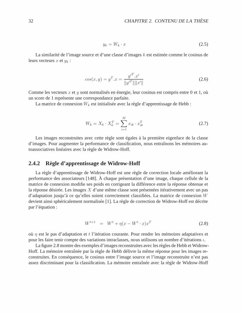
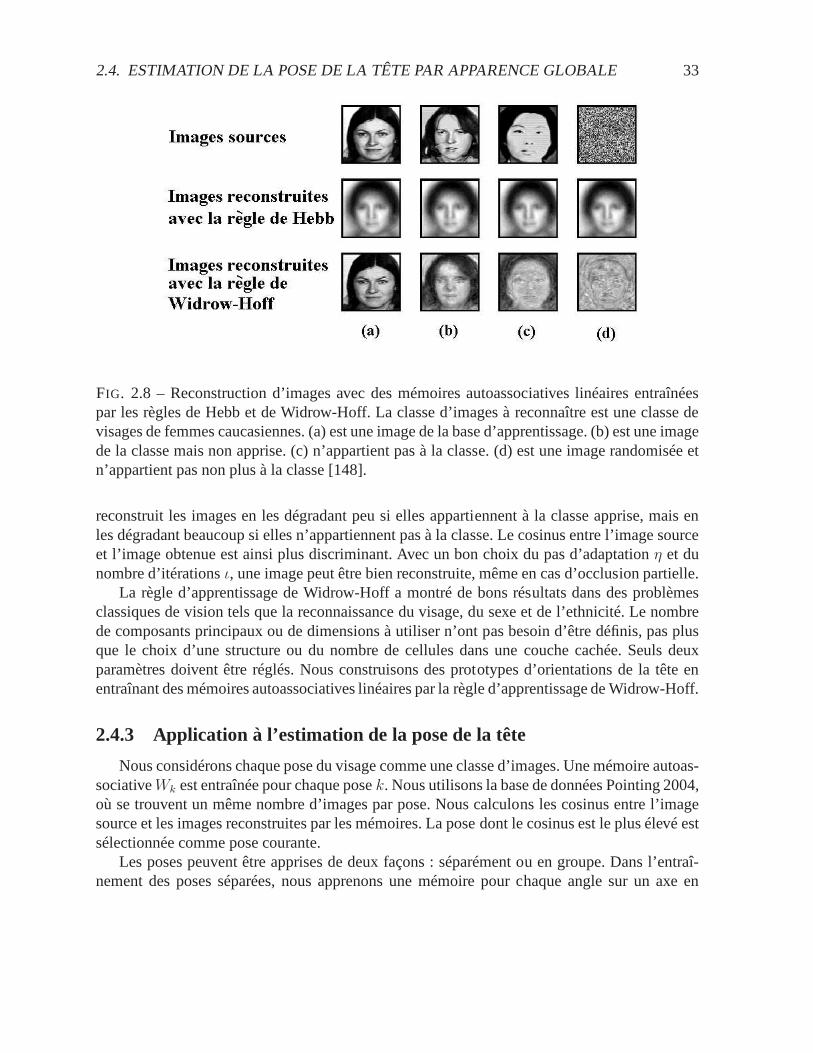


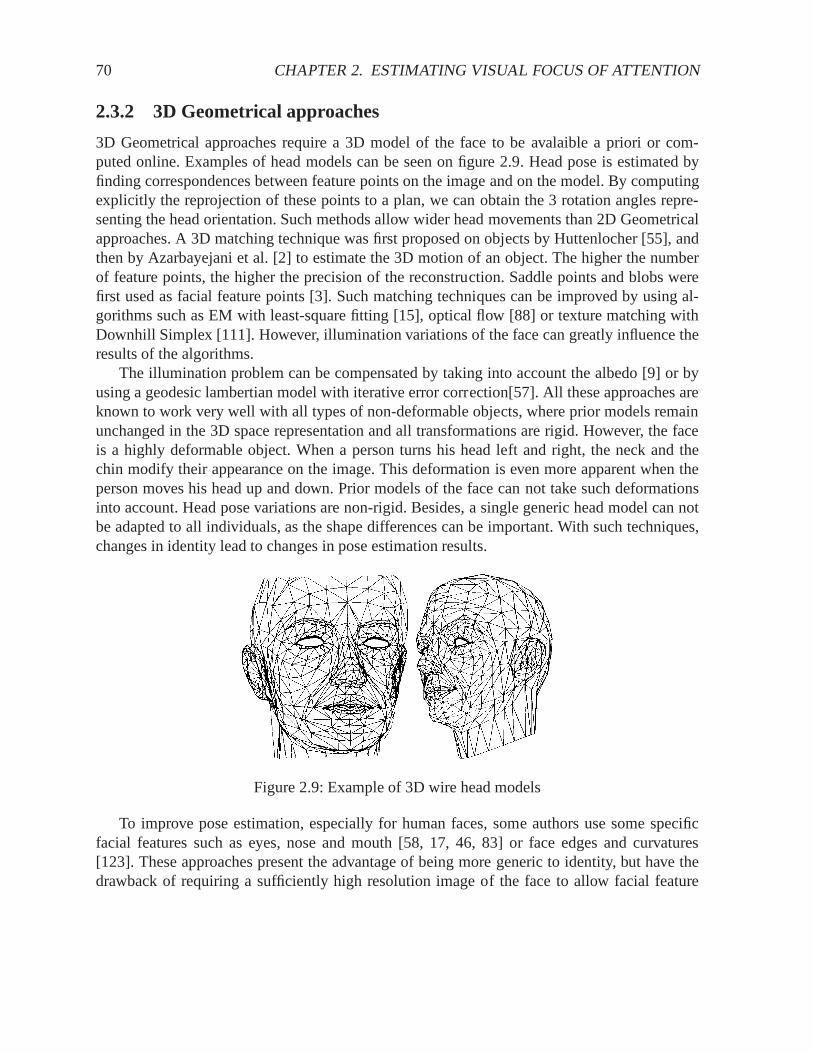


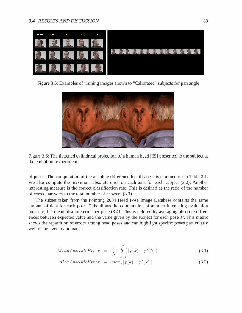


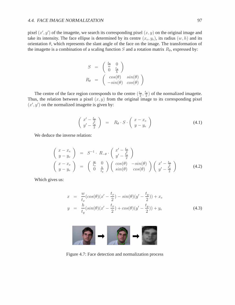
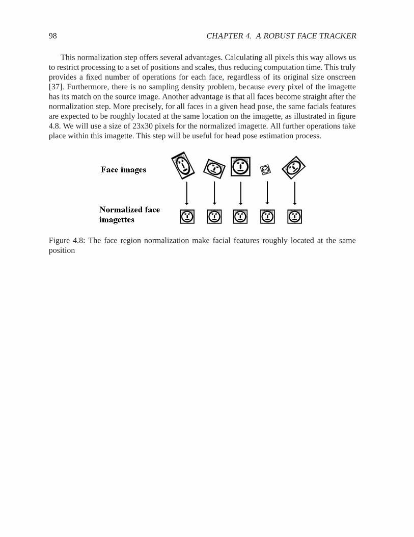


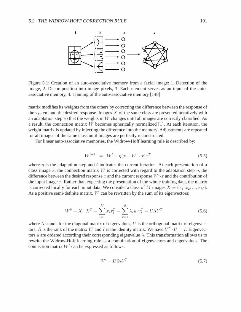


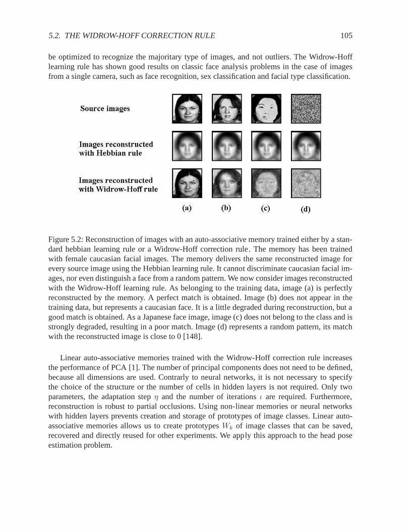


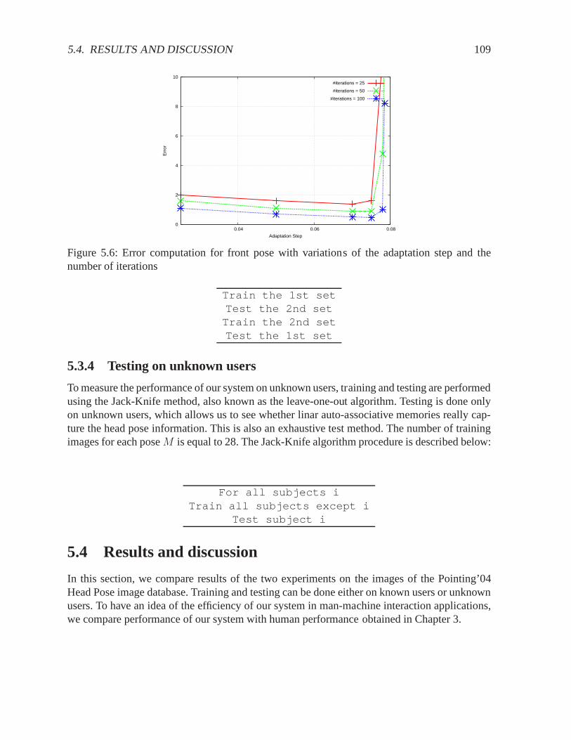


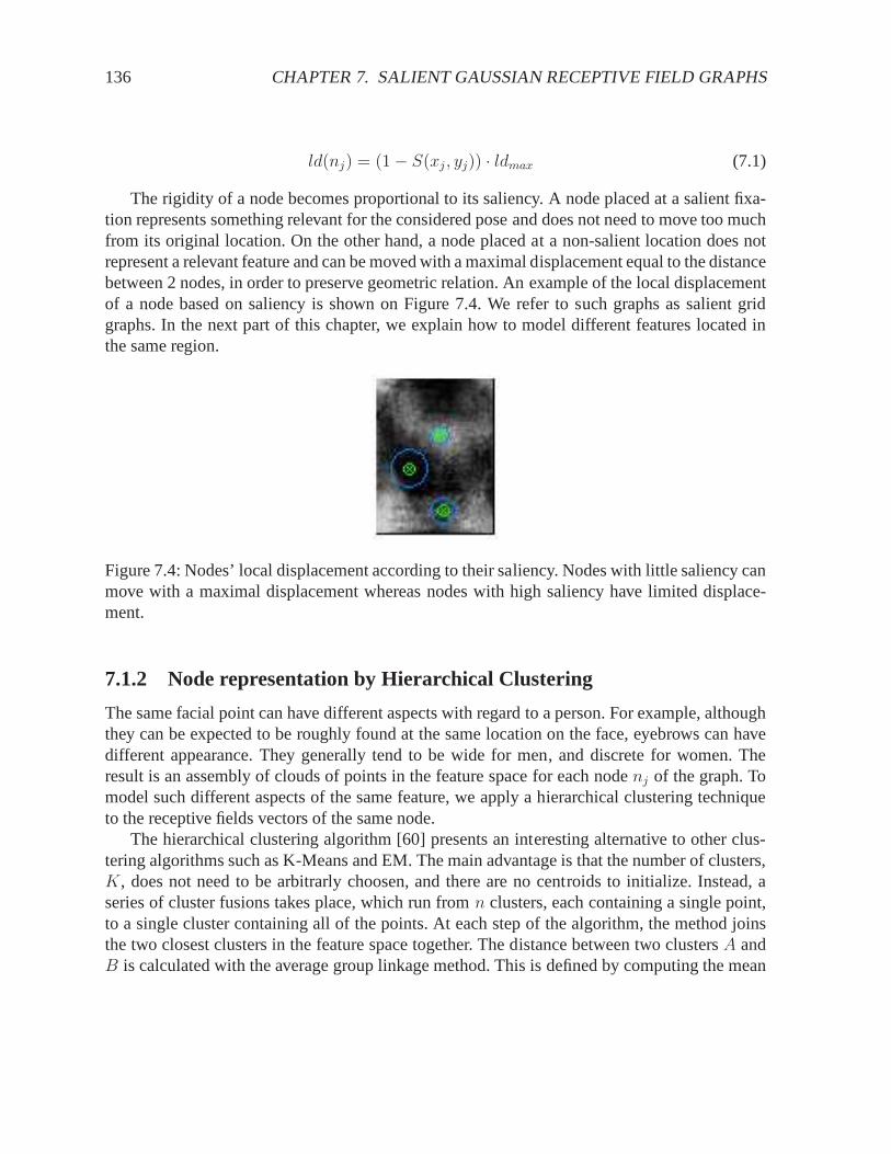


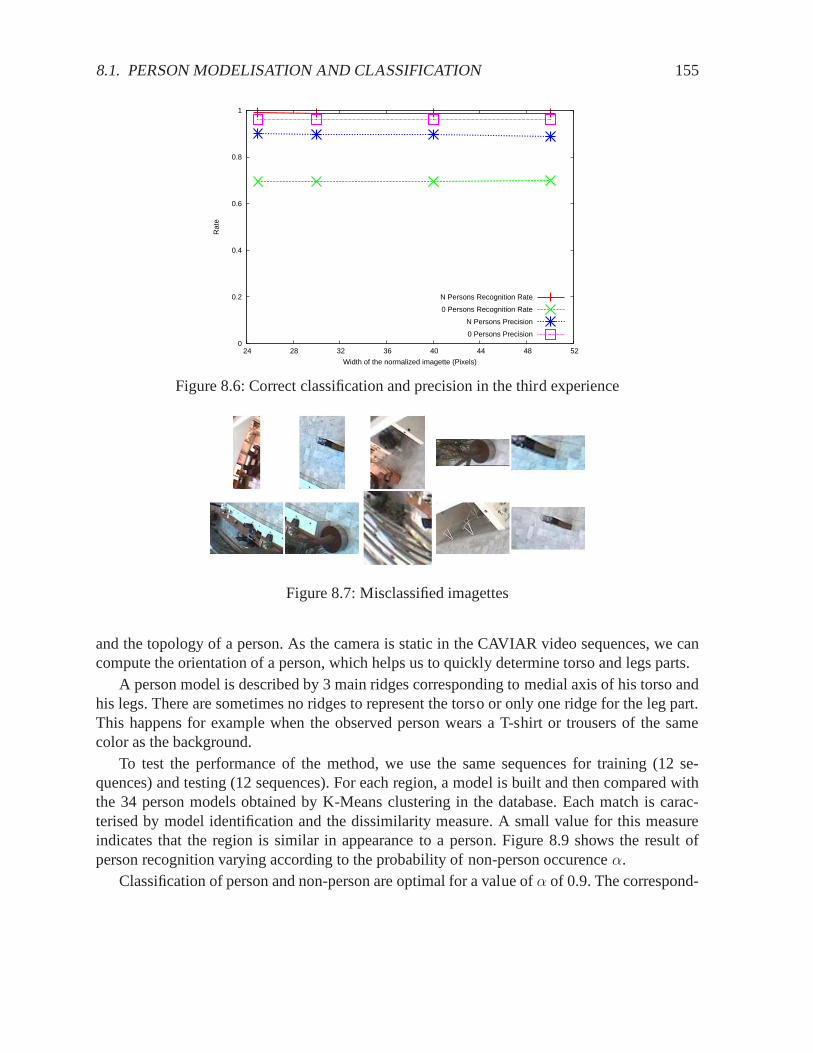


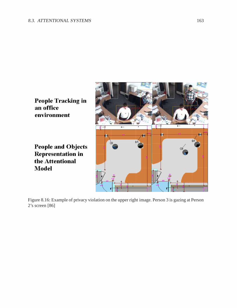


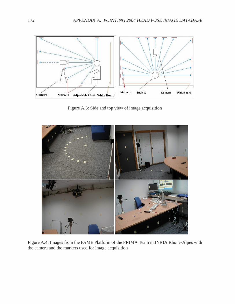


![Observation of surface superstructure induced by ...web.phys.ntu.edu.tw/nanomagnetism/eng/pdf/112-PRB95... · the structural model [viewing along the [111] direction, and with the](https://static.documents.pub/doc/80x56/5f5c2838b926626c3e3ca534/observation-of-surface-superstructure-induced-by-webphysntuedutwnanomagnetismengpdf112-prb95.jpg)

