129
MACRO ECONOMICS – 18KP1EC02 UNITS – 1, 2, 3, 4, 5 Dr. S. MANONMANI Assistant Professor Department of Economics KNGAC for Women (A) Thanjavur
MACRO ECONOMICS – 18KP1EC02 UNITS – 1, 2, 3, 4, 5
Dr. S. MANONMANI Assistant Professor
Department of Economics KNGAC for Women (A)
Thanjavur

UNIT – I NATIONAL INCOME AND ACCOUNTS
Introduction Economics is divided in to two areas 1. Micro Economics 2. Macro Economics Micro means small, Micro Economics is the analysis of the constituent
elements of an economy. Therefore Micro Economics is not aggregative but selective. It explains the working of the markets for individual commodities and the behaviour of individual buyer and seller.
Macro Economics is described as the economics of aggregates. Macro
Economics studies the ordinary businessof life in the aggregate, that is it studiesthe behaviour of economy as awhole. We study key variables like total output in the economy, the level of employment and unemployment, the aggregate price level, and national income.

National Income Definition: National income of a country can be
defined as the total market value of all final goods and services produced in the economy in a year.
Circular flow of Income In the monetary economy, there will be flows
of money corresponding to the flows of economic resources and flows of goods and services, each money flow is in the opposite direction to the real flow.
The Circular Flow of income in two sector Economy • Theory of circular flow of economic activities is a
fundamental assumption behind all macro economic theories.
• Lipsey defined the circular flow of income as “the flow of payments from domestic households to domestic firms and back again”.
• The circular flow can be explained with the help of example, in a simple economy which consists of four households, each households produces a different commodity. It is also assumed that there is only one rupee in the economy the flow of goods and money in this economy is illustrated in the following figure.

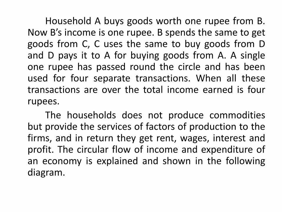
Household A buys goods worth one rupee from B. Now B’s income is one rupee. B spends the same to get goods from C, C uses the same to buy goods from D and D pays it to A for buying goods from A. A single one rupee has passed round the circle and has been used for four separate transactions. When all these transactions are over the total income earned is four rupees.
The households does not produce commodities but provide the services of factors of production to the firms, and in return they get rent, wages, interest and profit. The circular flow of income and expenditure of an economy is explained and shown in the following diagram.
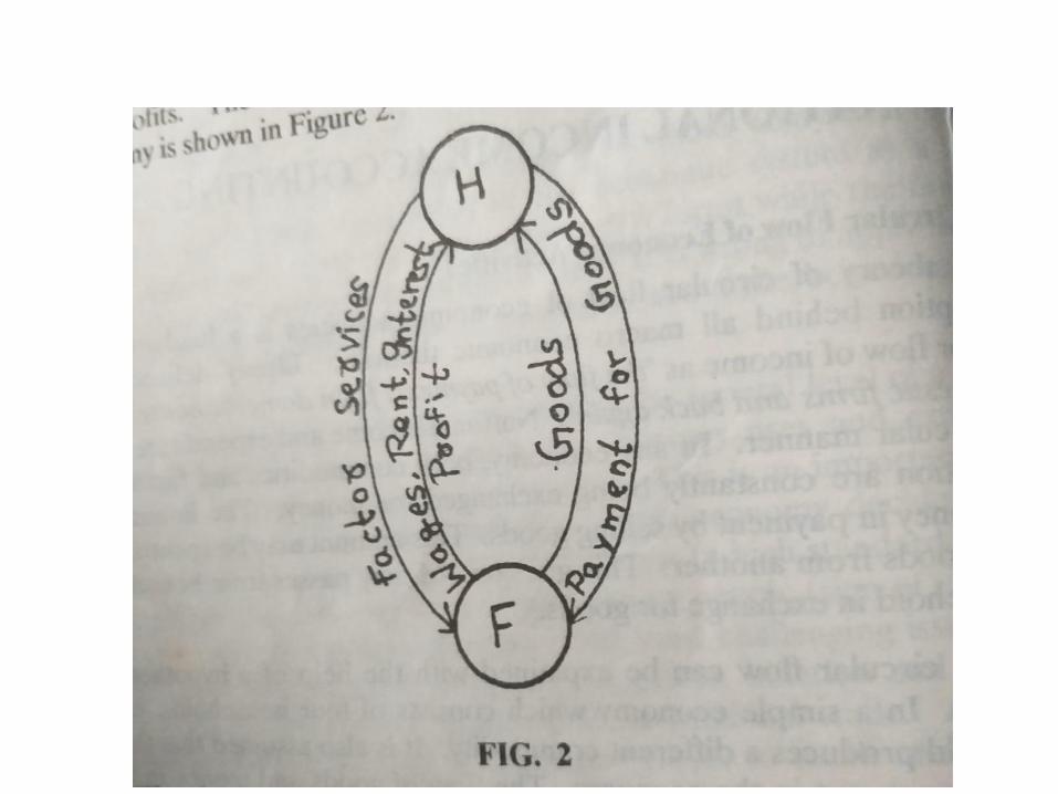

The business sector or firms get factor services from household sector and pays for their services. The household sector purchases goods from the business sector. Thus money paid to household becomes their income and money paid by household for purchase becomes income for firms. Therefore money flows from firm to household and back again.
This model of circular flow is so simple. The firms activities are in different stages. One firm;s output may become input for another firm, in such a case the circular flow is in the following way. It is assumed that the economy consists of three firms and several households.
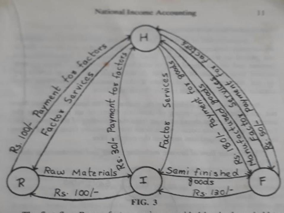

There are three firms R, I and F. The first firm R uses factor services from household by paying Rs. 100 and produce raw materials and sells these raw materials to Firm I. Firm I uses this raw materials and convert it into semi finished products, for this work it hires factor services from household by paying Rs. 30 and sells it to firm F for Rs. 130. Firm F employs factors from household by paying Rs. 50 and convert the semi finished product into finished products and sold to household for Rs. 180.
The total value of all sales by three firms are Rs. 410 (100+130+180). But the total value of the finished product is Rs. 180. (the value added by firms R,Iand F are Rs. 100+30+50).
The finished product is also known as social product. The social product of Rs. 180 is matched by the social income of Rs. 180. The equilibrium between social income and social product can be derived.

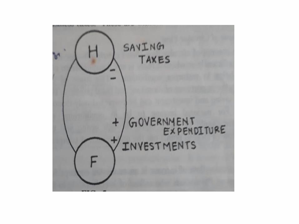
The circular flow with savings and investment A proper model of circular flow of income should take
into account withdrawals and injections. A withdrawal is any income that is not passes on into
the circular flow. Eg. If households earn income and do not spend it, similarly firms receive income from the sale of goods but do not spend it for factor services or do not distribute as profits. Withdrawals reduces the circular flow.
An injection is the addition to the income of the household that does not arise from the spending of domestic firms or an addition to the income of firms that does not arise from the spending of households. Eg. An injection occurs when firms borrow money from banks to pay hpusehold. Injection increases the circular flow.
The circular flow of income including saving and investment is explained from the following figure.


Savings by household or firms represent an important withdrawal. Household savings may be channelized by banks into the circular flow. Similarly firms may use their savings to build a new factory. Investment is an item of injection, it creates income for households.
The circular flow in a three sector economy
The three sector includes government activities. Which also affect the circular flow by withdrawing income as taxes and injecting income into spending. The following figure explains circular flow in a three sector economy.
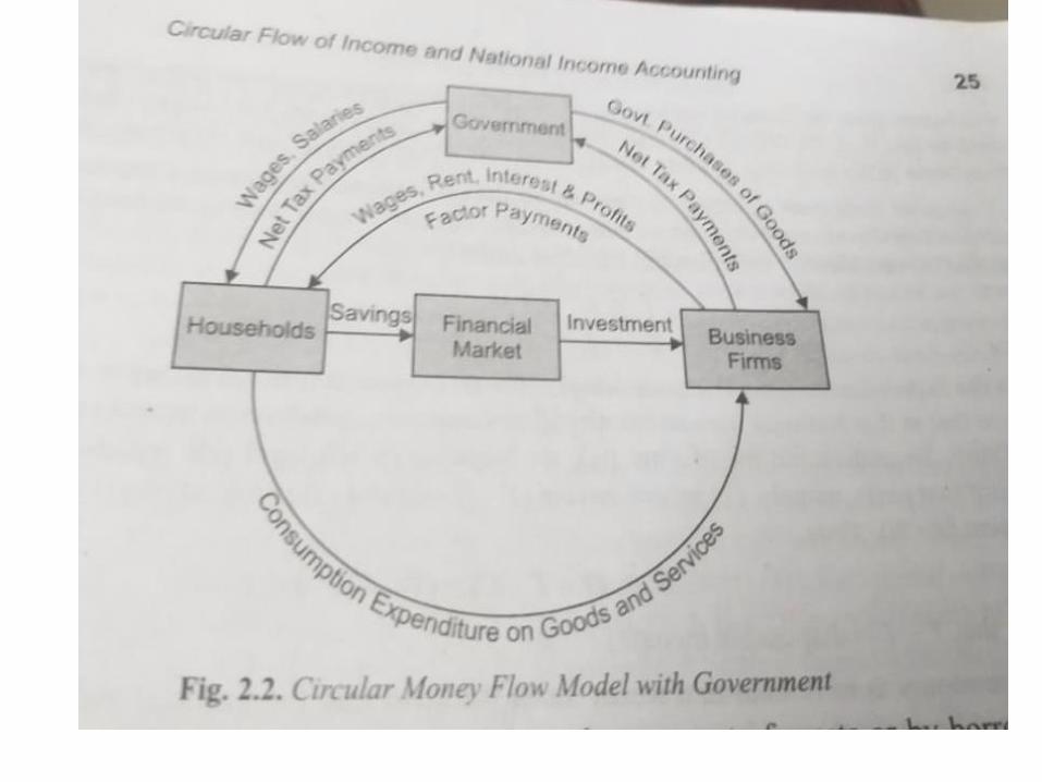
Taxes may be personal income tax, excise and sales tax or corporate business taxes. These are withdrawals from the circular flow.
Government may spend part of tax revenue to buy factor services from households or to buy goods and services from firms. Further govt. pay old age pensions, unemployment relief, sickness benefit etc. and also spends on education, health, housing, water facilities etc. All such govenment expenditures are injection into the circular flow.

The circular flow in a four sector economy
Four sector economy includes foreign trade which plays an important role in an open economy.
Import constitute a withdrawal from the circular flow because when households import, they are spending money for goods produced by foreign firm.
Exports are an injection into the economy. They create income for the domestic economy. The circular flow of four sector economy is shown in the following figure.
Savings, taxes and imports constitute withdrawals from the circular flow, investment, expenditure and exports are injection into the circular flow.


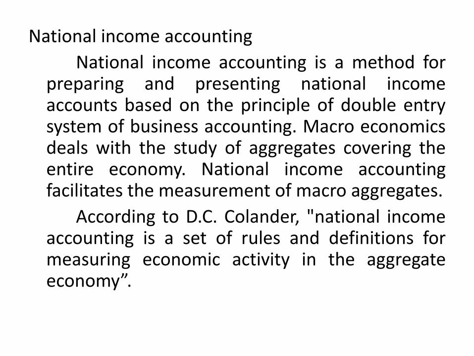
National income accounting
National income accounting is a method for preparing and presenting national income accounts based on the principle of double entry system of business accounting. Macro economics deals with the study of aggregates covering the entire economy. National income accounting facilitates the measurement of macro aggregates.
According to D.C. Colander, "national income accounting is a set of rules and definitions for measuring economic activity in the aggregate economy”.
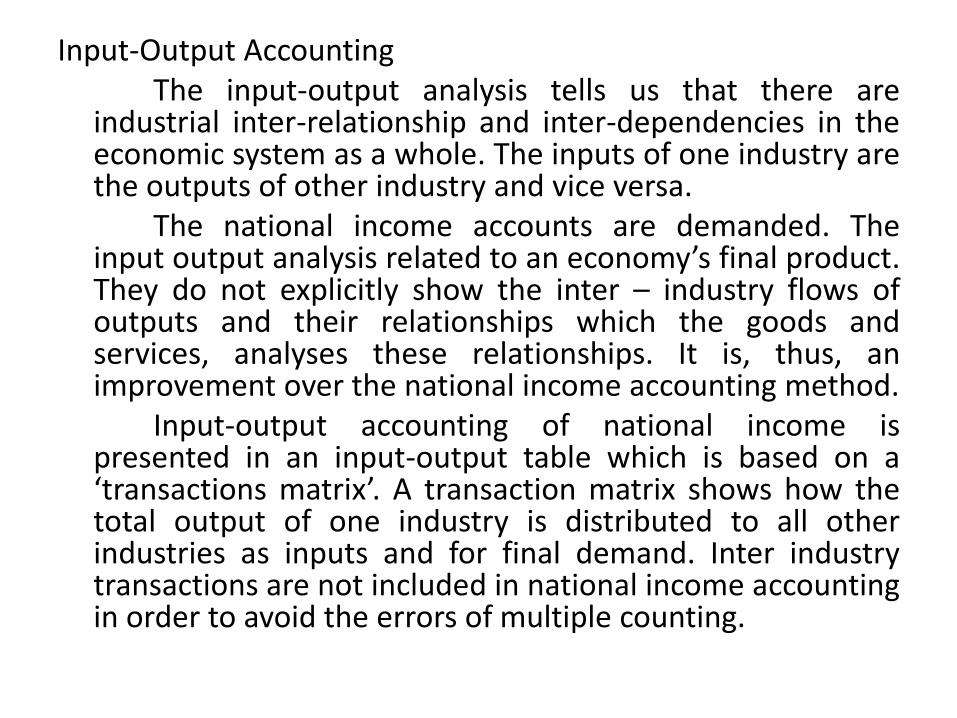
Input-Output Accounting The input-output analysis tells us that there are
industrial inter-relationship and inter-dependencies in the economic system as a whole. The inputs of one industry are the outputs of other industry and vice versa.
The national income accounts are demanded. The input output analysis related to an economy’s final product. They do not explicitly show the inter – industry flows of outputs and their relationships which the goods and services, analyses these relationships. It is, thus, an improvement over the national income accounting method.
Input-output accounting of national income is presented in an input-output table which is based on a ‘transactions matrix’. A transaction matrix shows how the total output of one industry is distributed to all other industries as inputs and for final demand. Inter industry transactions are not included in national income accounting in order to avoid the errors of multiple counting.

Only final demand or payments to factors enter into GNP at factor prices. The total resources available to economy are GNP plus imports, This is the Gross National Income(GNI). The GNI also the difference between total gross output and the total value of inputs.
Gross National Expenditure (GNE) is the sum of payments to satisfy final demand which includes exports, capital expenditure, and consumption expenditure.
Finally GNE = GNI.
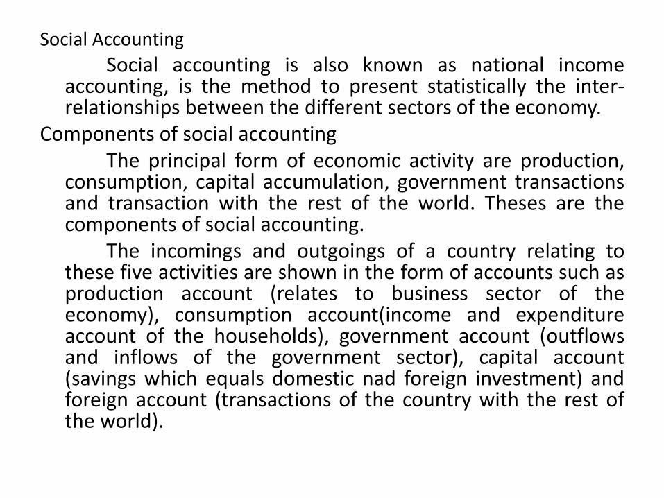
Social Accounting
Social accounting is also known as national income accounting, is the method to present statistically the inter-relationships between the different sectors of the economy.
Components of social accounting The principal form of economic activity are production,
consumption, capital accumulation, government transactions and transaction with the rest of the world. Theses are the components of social accounting.
The incomings and outgoings of a country relating to these five activities are shown in the form of accounts such as production account (relates to business sector of the economy), consumption account(income and expenditure account of the households), government account (outflows and inflows of the government sector), capital account (savings which equals domestic nad foreign investment) and foreign account (transactions of the country with the rest of the world).

Flow of funds Accounting The flow of funds accounts list the sources of all funds received and
the uses to which they are put within the economy. They show the financial transactions among different sectors of the economy and the link between savings and investment aggregates with lending and borrowing by them.
The account for each sector reveals all the sources of funds whether from income or borrowing and all the uses to which they are put for whether spending or lending. This way of looking at financial transactions in their entirely has come to be known as flow of funds approach.
In the flow of funds accounts, all changes in assets are recorded as uses and all changes in liabilities are recorded as sources. The flow of funds accounting system is presented in the form a matrix by placing sources and uses of funds statements of different sectors side by side. It reveals financial relationship among all sectors of the economy.
Two important point to be noted in this flow of funds account, first, financial Sources (net) and financial uses (net) of the economy must be equal. Second, Changes in assets (uses) and liabilities (sources) of each type of fund must be total up to zero.

Balance of payments Accounting
The Balance of Payments of a country is a systematic record of all its economic transactions with the outside world in a given year.
According to Bo Sodersten, ”The balance of payments is merely a way of listing receipts and payments in international transactions for a country”.
According to B.J. Cohen, ”It shows the country’s trading position changes in its net position as foreign lender or borrower and changes in its official reserve holding”.

The balance pf payments account of a country is constructed on the basis of double-entry book keeping. Each transaction is entered in the credit and debit side of the balance sheet. But balance of payments accounting differs from business accounting .
In business accounts debit ( - ) shown on the left side and credit ( + ) shown on the right side of balance sheet. But in balance of payments account credit is shown in the left side and debit is shown in the right side. When a payment is received from a foreign country, it is credit transaction while payment to a foreign country is a debit transaction.
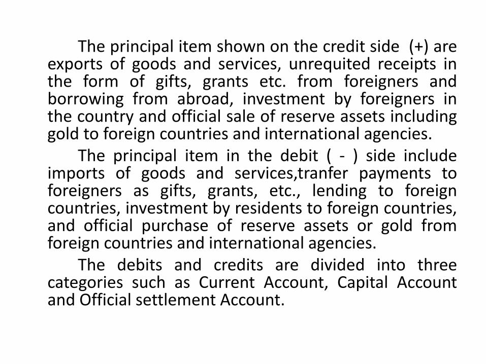
The principal item shown on the credit side (+) are exports of goods and services, unrequited receipts in the form of gifts, grants etc. from foreigners and borrowing from abroad, investment by foreigners in the country and official sale of reserve assets including gold to foreign countries and international agencies.
The principal item in the debit ( - ) side include imports of goods and services,tranfer payments to foreigners as gifts, grants, etc., lending to foreign countries, investment by residents to foreign countries, and official purchase of reserve assets or gold from foreign countries and international agencies.
The debits and credits are divided into three categories such as Current Account, Capital Account and Official settlement Account.
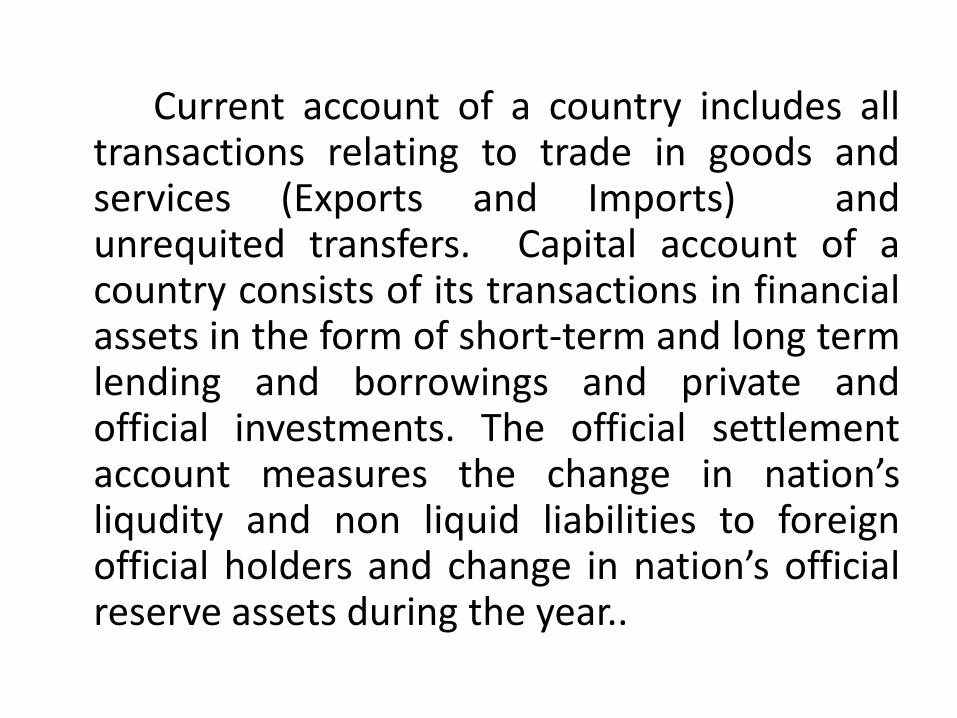
Current account of a country includes all transactions relating to trade in goods and services (Exports and Imports) and unrequited transfers. Capital account of a country consists of its transactions in financial assets in the form of short-term and long term lending and borrowings and private and official investments. The official settlement account measures the change in nation’s liqudity and non liquid liabilities to foreign official holders and change in nation’s official reserve assets during the year..
UNIT – 2 THEORY OF CONSUMPTION FUNCTION Consumption Function Meaning: Consumption function refers to the relationship
between consumption and general income. Keynes’ Consumption Function Keynes published his ‘General Theory’ in1936, laid
foundation for modern macro economics. According to Keynes, of all factors , the current level of income determines consumption of an individual and also of society. Since he laid stress on absolute size of current income as a determinant of consumption, his theory of consumption is also known as absolute income theory of consumption.

Keynes Psychological Law of Consumption Keynes Psychological law of consumption is the
basic importance in the analysis of income, output and employment. Keynes framed this law on the basis of the general psychology of the people that as income increases consumption expenditure will also increase. This psychological law based on three propositions.
1. When aggregate income increases consumption expenditure also increases
2. When income increases, the additional income is spent between consumption and saving.
3. When income increases, both consumption and saving increase but consumption increases less than proportionately.

Keynes psychological law of consumption based on the following assumptions,
1. The habits of the people regarding spending do not change. The propensity to consume remains stable.
2. Condition remains normal, there are no abnormal condition like hyper inflation, war etc.
3. The capitalistic laissez – faire economy prevailed in the country.
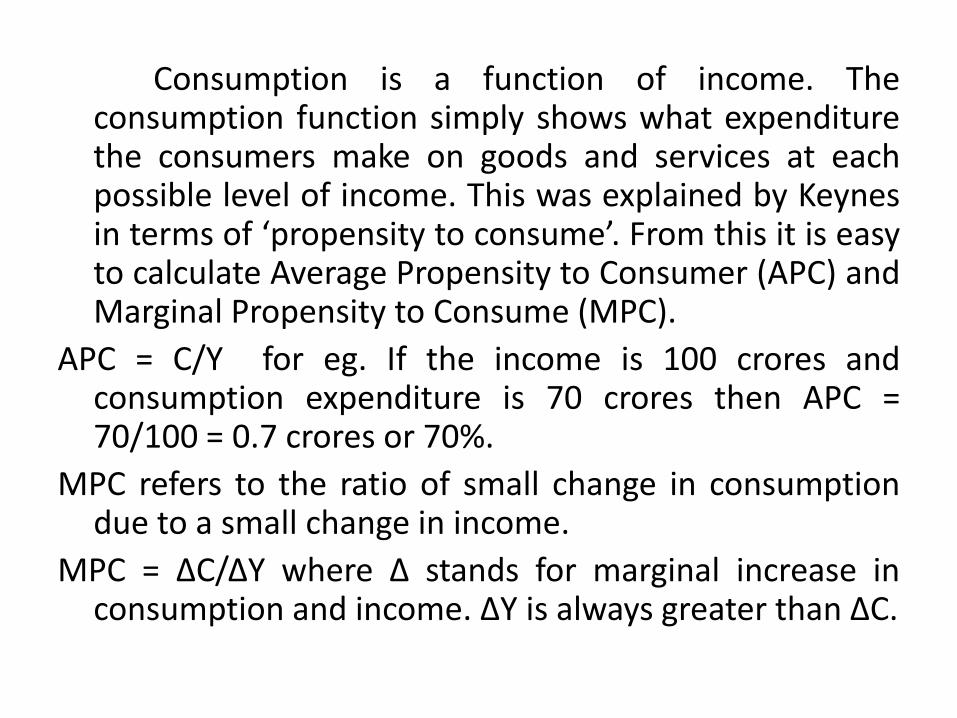
Consumption is a function of income. The consumption function simply shows what expenditure the consumers make on goods and services at each possible level of income. This was explained by Keynes in terms of ‘propensity to consume’. From this it is easy to calculate Average Propensity to Consumer (APC) and Marginal Propensity to Consume (MPC).
APC = C/Y for eg. If the income is 100 crores and consumption expenditure is 70 crores then APC = 70/100 = 0.7 crores or 70%.
MPC refers to the ratio of small change in consumption due to a small change in income.
MPC = ΔC/ΔY where Δ stands for marginal increase in consumption and income. ΔY is always greater than ΔC.

The following table will explain the relationship between APC and MPC
Income in Rs. Consumption in Rs.
APC = C/Y MPC =ΔC/ΔY
100 80 0.80 -
110 87 0.79 0.7
120 92 0.76 0.5
130 95 0.73 0.3
140 97 0.69 0.2
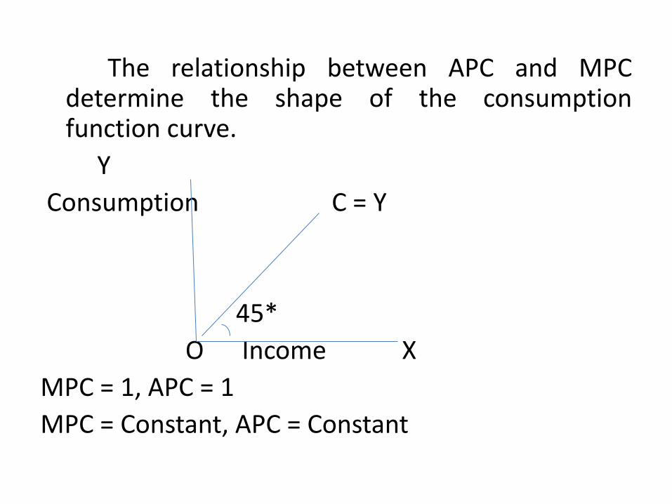
The relationship between APC and MPC determine the shape of the consumption function curve.
Y
Consumption C = Y
45*
O Income X
MPC = 1, APC = 1
MPC = Constant, APC = Constant

In case of linear consumption function (straight line) the MPC is positive but less than one and is often constant. The APC may be constant, declining or rising. These three possibilities give us three consumption function curves.
The first possibility is were every income is fully spent on consumption in which case the consumption function line will be a 450 line as shown in above figure.
In reality consumption function does not take this shape because the psychology of the people is such that when the income increases, they tend to spend only a portion and save atleast a little.
The other possible shapes of the consumption curves are as given in the following figures.


In figure A, MPC is constant but APC is falling. This is the most common type of consumption function and the APC is always greater than MPC. The general equation for this type of consumption function is C = a + bY, where a refers to the expenditure which is taking place even when there is no income. For example in figure A the consumption function curve starts a little high above the origin on the y axis. This is constant expenditure. After this level any increase in income is spent out a particular rate on consumption. Therefore MPC is constant and depicted as bY. Hence consumption function in this case is C = a + bY.
In figure B, both MPC and APC are constant and both are equal. Therefore consumption is always function of income alone. Figure C shows an increasing type of consumption function which is uncommon and has only theoretical validity. Thus the relationship between MPC and APC are responsible for the particular shape of consumption function curve.

From the above analysis we can observe three factors in the relationship between APC and MPC.
1. As income increases both MPC and APC decline but the decline in MPC is greater than the decline in APC.
2. MPC is higher in poorer countries than in richer countries. 3. MPC is always less than one. Properties of consumption function 1. The relationship between income and consumption is presented in
terms of real income and real consumption. The prices are assumed to be contant. The income is considered as disposable income that is after deducting taxes.
2. The relationship between C and Y can be expressed in the form of equation. The equation of the consumption function C = f (Y) is C = a + bY, where Cis consumption expenditure, Y is Income and a and b are constants, a is consumption even when income is zero (autonomous consumption) bi is marginal propensity to consume.Consumption function curves may also be curvi linear. Here an increase in incomewould mean a rise in consumption at a diminishing rate. In other words ΔC/ΔY goes on declining as income rising. The same equation C= a + bY may be used but the value of b will keep changing with the change in income as shown in the following figure.
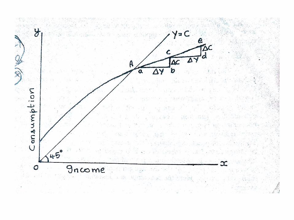

3. C/Y is the average propensity to consume, it may vary as the income level changes. In the above figure A is the break even point, where consumption and income are equal and net savings zero. Below the point consumption is greater than income and there is dissaving. Above the point consumption is less than income and there is positive net saving.
4. The ratio of change in consumption (ΔC) to change in income(ΔY) is the marginal propensity to consume, It is measured by the slope of the consumption function. In the above figure the MPC is indicated by reference to the triangle .
5. The fluctuations in the income and employment level are not due to changes in the consumption component of aggregate demand but due to the changes in investment component of aggregate demand.
6. The MPC is positive but less than unity. 7. The saving function is the counterpart to the consumption
function, S = Y – C. 8. 1 – ΔC / ΔY is marginal propensity to save and it is symbolised as
ΔS/ΔY.
Factors determining Consumption Function According to Keynes two principal factors, the subjective
factors and objective factors influence consumption function. The subjective factors are endogenous or internal and the objective factors are exogenous or external factors to the economic system.
The subjective factors are the psychological nature of human race. They are the outcome of individual and business motives.
There are eight psychological individual motives which determine individual’s spending.
1. The desire to keep reserve for emergency. 2. The desire to provide for old age and sickness 3. The desire to enjoy an enlarged future income through interest
and appreciation. 4. The desire to improve standard of living. 5. The desire to have financial independence. 6. The desire to do forward trading and speculation 7. The desire to bequeath a fortune. 8. The desire to satisfy a purely miserly instinct.
There are four business motives
1. Enterprise, the desire to do big things.
2. Liquidity, the desire to meet emergency successfully.
3. Income raise, the desire to secure larger income and to show successful management.
4. Financial prudence, the desire to provide adequate financial resources against depreciation, obsolescences and discharge debt.
these subjective factors remains constant during short run and keep the consumption function stable.

The objective factors are given by Keynes are, 1. Change in wage level: Increase in wage will increase consumption, the
consumption function curve will shift upward. A cut in wage will reduce consumption and shift the curve downward.
2. Windfall gains or losses: Unexpected gain will increase consumption and shift consumption function curve. Unexpected loss lead to the downward shifting of the consumption curve.
3. Changes in fiscal policy: The fiscal policy of the government relating to taxation, expenditure and public debt affect consumption.
4. Changes in expectations: If the consumers expect a shortage or rise in prices of certain goods they may rush to purchase such goods far in excess of their current needs.
5. Changes in rate of interest: If the interest rate is high the cost of holding money as liquid asset increases, people will find it less profitable to keep idle cash. They may invest, this will reduce total consumption and increase savings.
6. Financial policies of corporations: If corporations and companies retain more reserves and give lesser profits in the form of dividends, the disposable income of the shareholders will be smaller.

7. Holding of liquid assets: Liquid assets in the form of cash balances, savings and government bonds in the hands of consumers also influences consumption function. If the people hold larger liquid assets the propensity to consume will move upward and vice versa.
8. The distribution of income: If the income distribution is more even, then the propensity to consume will be high.
9. Attitude towards saving: If the consumers value future consumption more than present consumption, they will tend to save more and consume less and the consumption function curve will shift downward.
10. Duesenberry hypothesis: According to James Duesenberry the expectation of an individual depends not on his current income but also on his past income and standard of living. Even if the current is reduced , the individual might continue to spend the same amount on current consumption, out of past saving.
11. Selling effort.: Selling cost and advertisement may increase the consumption of one good at the cost of other,
12. Changes in relative prices: Changes in relative prices increase demand for some products at the expense of other products.
13. Volume of wealth: The larger the wealth possessed by an individual the higher will be the propensity to consume.
14. Demographic factors: Factors like size of the family, stage in the family life cycle, place of residence, occupation etc., affect consumption function.
15. Terms of consumer credit: Easy availability of credit will in crease the propensity to consume of consumer durables.
16. Permanent income; It is also known as national income. A family’s expenditure on current expenditure on consumption determined not only by by its cuurent income but also its permanent income. If the later is more, consumption function will be more.
17. Pigou effect: The changes in the real value of liquid assets also affect consumption function. This is known as pigou effect.

Theories of Consumption Function
In the post war period several economists empirically tested the relationship between income and consumption. They made use of both cross-section data and time series data in this connection. Cross section data showed that rich households had a smaller APC than the poor ones. The time series data showed that for different periods different consumption function could be derived. These different consumption functions are shown in the following figure.

Three types of theoretical explanations, have been offered by the economists who sought to reconcile the short run and long-run relationships between aggregate consumption and aggregate disposable income. They are,
1. Absolute income hypothesis – J. M. Keynes 2. Relative income Hypothesis _ James Dusenberry 3. Permanent Income Hypothesis: Milton friedman. 4. Life cycle hypothesis – Franco Modigliani. Absolute Income Hypothesis Keynes consumption income relationship is known as
the absolute income hypothesis. It states that when income increases consumption also increases but by less than the increase. This means that the consumption income relationship is non proportional. James Tobin and Arthur Smithies tested the hypothesis in separate studies.

Tobin tested the relationship between consumption and absolute income as suggested by Keynes with three kinds of budget data. 1. Budget of the same families over three successive years. 2. Budgets of black and white families in the same cities in the same year. 3. Budgets of families in different cities in the same year. With the help of these tests he made the following observations.
1. In all three tests, the absolute income interpretation proved to explain the observations better than the alternative theories.
2. However, in the case of budgets of black and white families in the same cities in the same year, net saving was found to depend on assets holdings as well as income
3. Absolute level of income determine saving rates, but the existence of asset holdings by consumers tend to depress the propensity to save.
The absolute income hypothesis also suggests that non-income factors would shift the consumption function upward with time.
1. Since the end of second world war, a variety of new household consumer goods have come into existence at arapid rate. The introduction of such essential tends to shift the consumption function upward.
2. Since the post war period, there has been an increased tendency towards urbanisation, This shift the consumption function upward because the propensity to consume of the urban wage earners is higher than that of the farm workers.
3. There has been a continuous increase in the percentage of old people in the total population in the long run
Factors like these according to the absolute income theory have caused the consumption function to shift upward by roughly the amount necessary to produce a proportional relationship between consumption and income over the long run.
The absolute income hypothesis is explained in the following figure.


In this figure, X axis measure income and Y axis consumption, C1 is the long run consumption function which shows the proportional relationship between consumption and income as we move along the long run curve. For instance the APC and MPC are equal at point A and b on this curve. CO1 and CO2 are the short-run consumption functions. But due to the factors mentioned above, they tend shift upward from point A to point B along the long run consumption functions CO1 and CO2 would cause consumption not to increase in proportion to the increase in income.
The great merit of this theory is that it lays stress on the factors other than income which affect the consumer behavior.
Relative Income Hypothesis This hypothesis was formulated by James Duesen berry. This
hypothesis is based on the following assumptions. 1. Every individual’s consumption behavior is interdependent
(Demonstration Effect) 2. Consumption relations are not reversible in time (Ratchet effect). Demonstration effect According to Duesenbeery consumption and savings decision
are greatly influenced by the social environment in which one lives. The social environment refers to the tendency of the individuals not only to keep with the Jonses but also to surpass the Joneses. An individual normally spends in order to keep and maintain a certain economic status with in the neighbourhood. The consumer’s preferences are interdependent. A rich man will have a lower APC because he will need a smaller portion of his income to maintain his consumption pattern. The poor man will have a higher APC because he tries to keep up with the consumption standards of his neighbours.
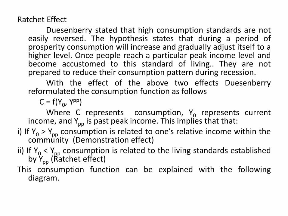
Ratchet Effect Duesenberry stated that high consumption standards are not
easily reversed. The hypothesis states that during a period of prosperity consumption will increase and gradually adjust itself to a higher level. Once people reach a particular peak income level and become accustomed to this standard of living.. They are not prepared to reduce their consumption pattern during recession.
With the effect of the above two effects Duesenberry reformulated the consumption function as follows
C = f(Y0, Ypp) Where C represents consumption, Y0 represents current
income, and Ypp is past peak income. This implies that that: i) If Y0 > Ypp consumption is related to one’s relative income within the
community (Demonstration effect) ii) If Y0 < Ypp consumption is related to the living standards established
by Ypp (Ratchet effect) This consumption function can be explained with the following
diagram.

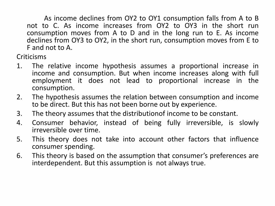
As income declines from OY2 to OY1 consumption falls from A to B not to C. As income increases from OY2 to OY3 in the short run consumption moves from A to D and in the long run to E. As income declines from OY3 to OY2, in the short run, consumption moves from E to F and not to A.
Criticisms 1. The relative income hypothesis assumes a proportional increase in
income and consumption. But when income increases along with full employment it does not lead to proportional increase in the consumption.
2. The hypothesis assumes the relation between consumption and income to be direct. But this has not been borne out by experience.
3. The theory assumes that the distributionof income to be constant. 4. Consumer behavior, instead of being fully irreversible, is slowly
irreversible over time. 5. This theory does not take into account other factors that influence
consumer spending. 6. This theory is based on the assumption that consumer’s preferences are
interdependent. But this assumption is not always true.

The Permanent Income Hypothesis
The explanation of the short and long period data has been provided by Milton Friedman, Who argues that the consumption function is essentially proportional.
According to him there is no tendency for the proportion of income saved to increase at higher income levels. He rejects the use of current income as the determinant of consumption expenditure.
He divides the consumption and income into ‘permanent’ and ;transitory; components, so
Ym = Yp + Yt and
Cm = Cp + Ct
where Y stands for income and C stand for consumption and m,p and t are for their measured permanent and transitory components.
Permanent income is the means of income which is regarded as permanent by the consumer. It depends on time and farsightedness. It includes non-human wealth like personal attributes of the earners. Y being measured income or current income it may be larger or smaller than his permanent income. In any period.
The difference between measured and permanent income are due to transitory component of income.(Yt). The transitory income may rise or fall depending on the cyclical variations.
If the transitory income is positive, the measured income will be higher than the permanent income. If it is negative it will be lower than the permanent income.. The transitory income can also be zero in which case the measured income is equal to permanent income.

Permanent consumption is the amount planned to consume in a given pewriod. Measured consumption is divided into permanent consumption (Cp) and Transitory consumption (Ct). If the transitory consumption is positive the measured consumption may be more than permanent consumption. If the transitory consumption is negative, it will be less than permanent consumption. If the transitory consumption is zero, it will be equal to permanent consumption.
Permanent consumption is a multiple (K) of permanent income (Yp). Cp = Kyp and K = f(r,w,u) Therefore Cp = K(r,w,u) Yp Where K is the function of the rate of interest ®, the ratio of income to
wealth (w) and the consumer’s propensity to consume (u). This equation tell us that in the long period consumption increases in proportion to change in Yp.
The relationship between the permanent and transitory components of income and consumption are based on the following assumptions.
1. There is no correlation between transitory and permanent incomes. 2. There is no correlation between permanent and transitory consumption. 3. There is no correlation between transitory consumption and transitory income. 4. The differences in permanent income alone affect consumption. The permanent income hypothesis can be explained with the help of following
diagram.
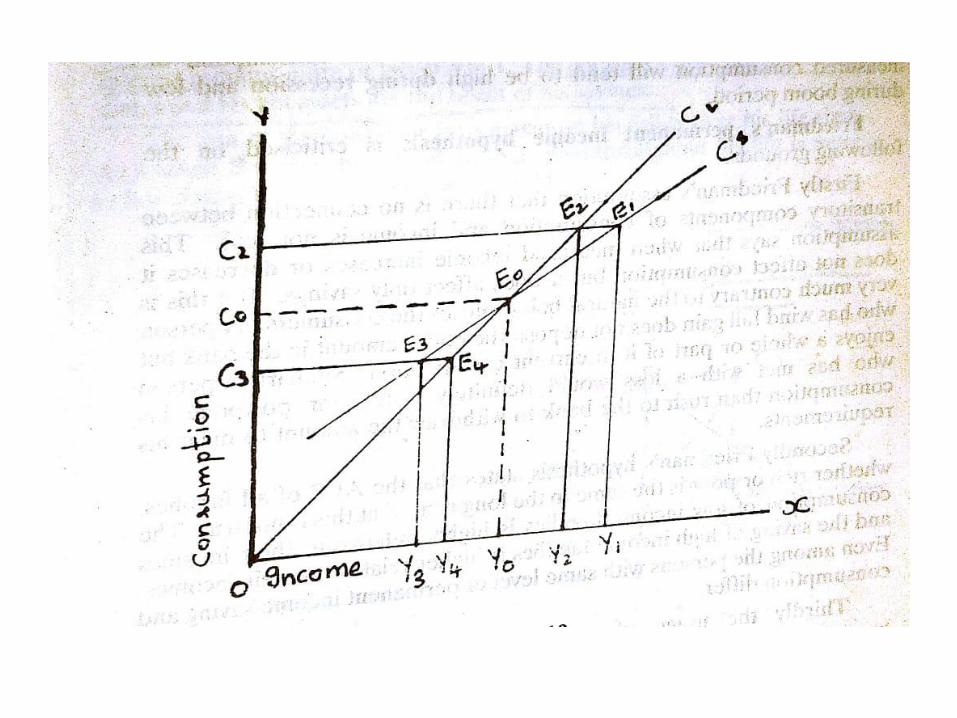

X axis measure income and Y axis measures consumption. CL is the long run consumption function and CS is the short run consumption function. At Oy0, income level Cs and CL coincide at point E0. At this point the changes in permanent income and measured income are identical. Therefore the permanent and measured consumption are shown by OC0. If we move to the left of point E0 on the CS curve at E3 the measured income decline to OY3 due to negative transitory income component. As the permanent income OY4 is higher than the measured income OY3, permanent consumption will remain at OC.
If we move to the right of point E0 on the CS curve at E1 shows the measured income to be OY1. Here the measured consumption is OC2. But OC2 level of consumption can be maintained permanently at the permanent income level OY2.
Thus Y1 Y2 is the positive transitory income component measured income OY1, which is higher than the permanent income OY2.
Friedman’s permanent income hypothesis suggests that current consumption or measured consumption will tend to high during recession and low during boom period.
Criticisms
1. Friedman’s assumption that there is no connection between transitory components of consumption and income is not real.
2. Friedman’s hypothesis states that the APC of all families, whether rich or poor is the same in the long run. This is not true.
3. The usage of the terms like permanent, transitory and measured have tended to affect the clarity of the theory.
4. The distinction between human and non-human wealth is missing.
The Life Cycle Hypothesis The hypothesis that attempts to explain the difference between the long
run and cyclical consumption is developed by Albert Ando and Franco Modigliani. It is termed as Life Cycle Hypothesis. This hypothesis persumes the cyclical variations in the income of an individual over his life time. At the beginning of his working age income is relatively low, in the middle years it is relatively high and at the end of the working span it is relatively low again. Though the level of income varies over his life cycle, yet the aggregate consumption expenditure remains a constant proportion of income.
This hypothesis is based on the following assumptions. 1. There is no change in the price level during the life of the consumer. 2. The rate of interest remains more or less stable. 3. The consumer does not inherit any assets and his net assets are the
result of his savings. The aim of the consumer is to maximise his utility over his life time.
As a result of consumption of an individual throughout his life is more or less constant. This is explained in the following diagram.

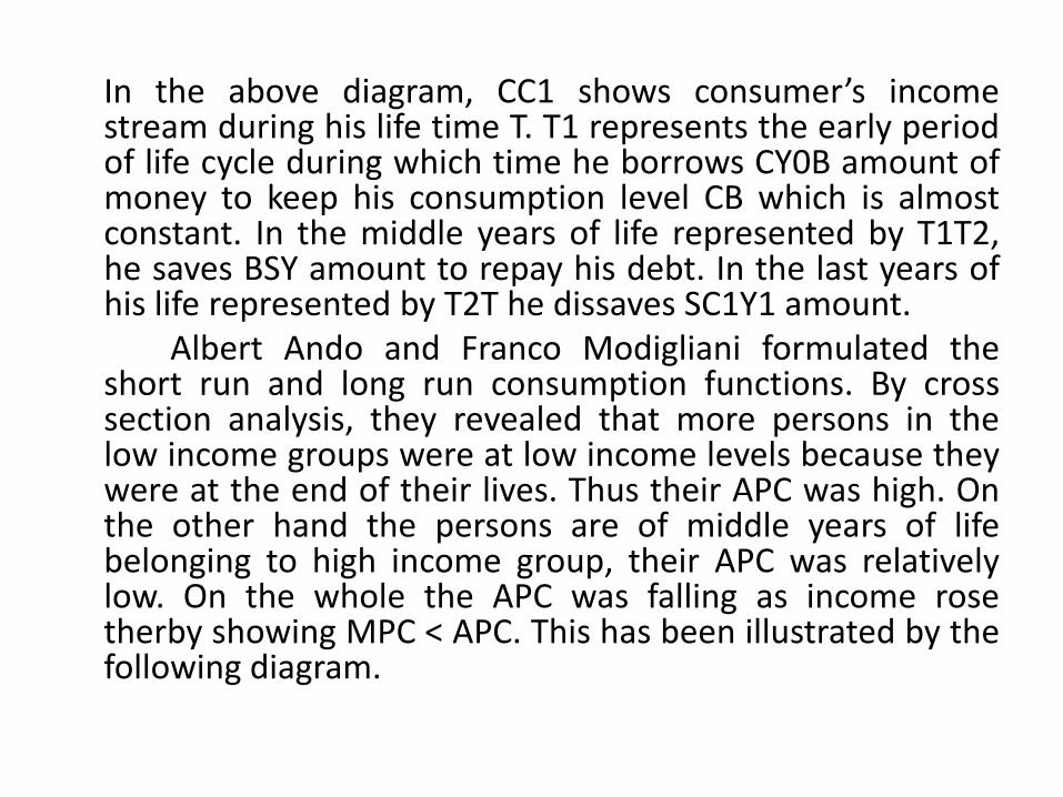
In the above diagram, CC1 shows consumer’s income stream during his life time T. T1 represents the early period of life cycle during which time he borrows CY0B amount of money to keep his consumption level CB which is almost constant. In the middle years of life represented by T1T2, he saves BSY amount to repay his debt. In the last years of his life represented by T2T he dissaves SC1Y1 amount.
Albert Ando and Franco Modigliani formulated the short run and long run consumption functions. By cross section analysis, they revealed that more persons in the low income groups were at low income levels because they were at the end of their lives. Thus their APC was high. On the other hand the persons are of middle years of life belonging to high income group, their APC was relatively low. On the whole the APC was falling as income rose therby showing MPC < APC. This has been illustrated by the following diagram.

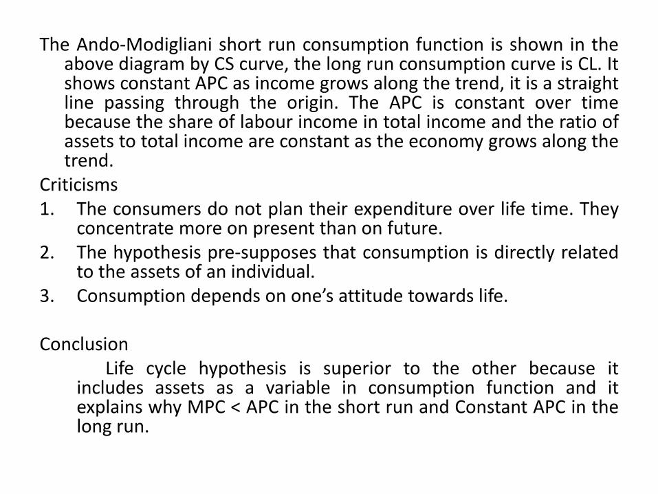
The Ando-Modigliani short run consumption function is shown in the above diagram by CS curve, the long run consumption curve is CL. It shows constant APC as income grows along the trend, it is a straight line passing through the origin. The APC is constant over time because the share of labour income in total income and the ratio of assets to total income are constant as the economy grows along the trend.
Criticisms 1. The consumers do not plan their expenditure over life time. They
concentrate more on present than on future. 2. The hypothesis pre-supposes that consumption is directly related
to the assets of an individual. 3. Consumption depends on one’s attitude towards life.
Conclusion Life cycle hypothesis is superior to the other because it
includes assets as a variable in consumption function and it explains why MPC < APC in the short run and Constant APC in the long run.

UNIT – 3 INVESTMENT FUNCTION
Meaning
In ordinary terms, investment means purchase of shares, stocks, bonds and securities which are already exists in stock market. This is called financial investmenmts. But according to Keynes investment refers to real investment which adds to capital equipment. It leads to increase in income and production.
Types of investment
There are three types of investment. They are,
1. Business fixed investment
2. Residential investment
3. Inventory investment
Business Fixed Investment
Investment in the machines, tools and equipment that businessmen by for use in further production of goods and services is business fixed investment. The expenditure made on the machines, equipment etc. continues to be used for production for a relatively long time.
Keynes states that Business fixed investment is determined by expected rate of profit (Which he calls Marginal Efficiency of Capital) and rate of interest. According to the neoclassical theory, business fixed investment is determined by marginal product of capital in one hand and user’s cost of capital on the other.

Residential Investment
Residential investment refers to expenditure which people make on construction or buying houses. Residential investments depend on price of existing housing units. The price of housing units determined by demand for it, in the long run the price is determined by rate of population and formation of new households.
Inventory investment
Firms hold inventories of raw materials, semi finished goods and finished goods to be sold shortly. The change in the inventories or stocks of these goods with the fiems is called inventory investment.
The other types
1. Real Investment
i. Induced investment
ii. Autonomous Investment
iii. Gross investment
iv. Net investment
Induced Investment
Induced investment is profit motivated. It is influenced by factors like demand, prices, wages, and interest. For example, when income increases the demand for consumption goods will increase, to meet this increased demand investment will increase. Induced investment is a function of income that is I = f(Y). It is income elastic and increases or decreases with income.
Autonomous Investment
Investments made by the government on public utilities are autonomous investment, it is not profit motivated. Since investment on these projects are generally associated with public policy it is called public investment. It is influenced by exogenous factors like innovations, inventions, population, weather, war etc. It is not influenced by demand but it influences demand. Autonomous investment is independent of the level of income. It is income inelastic.
Gross investment: Investment to replace depreciated capital assets.
Net investment: Net addition to the volume of capital in the form of new business premises, new machinary and storesect.

Determinants of Investment – Keynes’ Theory The classical economists believed that investment depended on rate of interest. According
to Keynes investment depends on marginal efficiency of capital and rate of interest. Marginal Efficiency of Capital (MEC) MEC refers to the expected profitability of a capital asset. It may be defined as the highest
rate of return over expected cost from the marginal or additional unit of a capital asset. MEC depends on two factors 1. The prospective yield of the capital asset. 2. The supply price of the capital asset. MEC is the ratio of these two factors. The prospective yield of a capital asset is the total net
return from the asset over its life time. Marginal Efficiency of Capital is the percentage profit expected from a given investment on a
capital asset. For eg. If the supply price of a capital asset is Rs. 20000 and its annual yield is Rs. 2000, then
marginal efficiency of the asset is 2000/20000 X 100 = 10 percent. Marginal Efficiency of Capital and Rate of Interest The private investment depends on MEC and rate of interest. The rate of interest is
determined by demand and supply. On the demand side it is determined by liquidity preferences and on the supply side the money available in the economy.
As long as the MEC is greater than the rate of interest the investor will invest till the MEC and the rate of interest get equalised..
The relationship between investment and rate of interest is shown in the following figure 1. The following figure 1 shows trhat given MEC, a fall in the rate of interest will increase the investment demand and a rise in the rate of interest will decrease the investment demand.
The second figure shows shift in MEC.


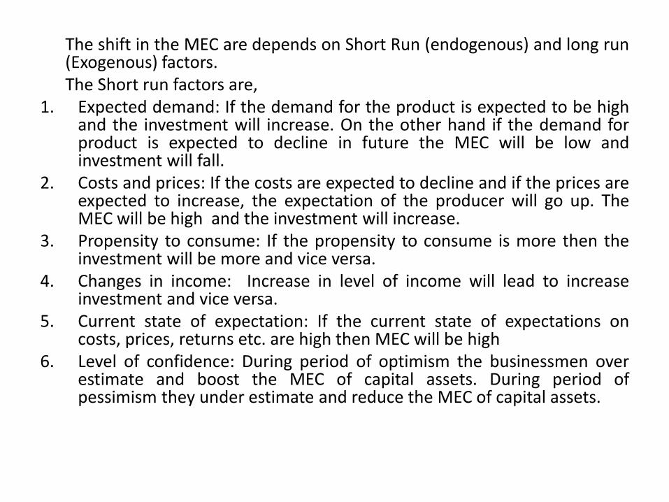
The shift in the MEC are depends on Short Run (endogenous) and long run (Exogenous) factors.
The Short run factors are, 1. Expected demand: If the demand for the product is expected to be high
and the investment will increase. On the other hand if the demand for product is expected to decline in future the MEC will be low and investment will fall.
2. Costs and prices: If the costs are expected to decline and if the prices are expected to increase, the expectation of the producer will go up. The MEC will be high and the investment will increase.
3. Propensity to consume: If the propensity to consume is more then the investment will be more and vice versa.
4. Changes in income: Increase in level of income will lead to increase investment and vice versa.
5. Current state of expectation: If the current state of expectations on costs, prices, returns etc. are high then MEC will be high
6. Level of confidence: During period of optimism the businessmen over estimate and boost the MEC of capital assets. During period of pessimism they under estimate and reduce the MEC of capital assets.

The long run factors are, 1. Population growth: A rapidly growing population will increase the
demand for all types of goods. 2. Development of new areas: When a new area is developed heavy
investments in all fields such as agriculture, industries, electricity, housing etc. are to be undetaken.
3. Technological factors: New inventions may insists the installation of new machineries and increase investment.
4. Productive capacity of the industry: If the exisisting capacity is fully utilise then any further increase in demand will be met by making fresh investments.
5. Level of current investment: If the existing level of investment is already high there will be little scope for further investment.
Criticisms of MEC 1. Keynes used the term marginal efficiency of capital in a vague manner. 2. Keynes failed to recognise that the interest rate are also governed by
expectations. 3. He considered MEC in the field of dynamics economics and the rate of
interest in the field of static economics.

The Rate of Interest The rate of interest is the second important factor determining the volume
of investment. Keynes propounded ‘Liquidity Preference Theory’ to explain rate of interest. According to Keynes, the rate of interest is purely a monetary phenmenon and it is determined by supply of and demand for money. Liquidity preference depends on three motives. They are,
1. Transaction motive 2. Precautionary motive 3. Speculative motive Transaction Motive It refers to the demand for money for current transactions by households and
firms. Households have to keep certain amount of money to carry on their day to day activities. This amount depends on the size of income, method of expenditure and the time interval after which the income is received. This is called income motive.
The business motive refers to the needs of the firm to keep cash in order to meet their current needs like payment of wages, purchase of raw materials, transport charges etc. The demand for money by firms also depends on income, level of business activity etc.
The transaction demand for money depends on income M1 = f(Y) Where MI1 is the transaction demand for money and f(Y) is the function of income.

Precautionary motive Households and business firms need more money because they
have to take precautions against unforeseen emergencies like sickness, accidents, fire, theft and unemployment. Whether it is an individual or firm the amount of money need to satisfy precautionary motive is the function of income. Since both the transaction and precautionary motive depends on income, Keynes put them together. Thus M1 + M2 = L1 = f(Y).
Speculative Motive The third and most important motive is speculative demand for
money. People keep cash because they want to take advantage of the changes in prices of bonds and securities. The amount of money which the people wish to hold for speculative motive depends on the expected change in the rate of interest.
L2 = f(r) Where L2 is the speculative demand for money and f(r) is the expected
change in the rate of interest. The higher the rate of interest, the less shall be the demand for money
in the form of idle cash balances and vice-versa.
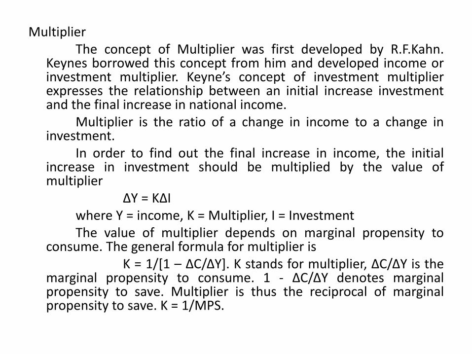
Multiplier The concept of Multiplier was first developed by R.F.Kahn.
Keynes borrowed this concept from him and developed income or investment multiplier. Keyne’s concept of investment multiplier expresses the relationship between an initial increase investment and the final increase in national income.
Multiplier is the ratio of a change in income to a change in investment.
In order to find out the final increase in income, the initial increase in investment should be multiplied by the value of multiplier
ΔY = KΔI where Y = income, K = Multiplier, I = Investment The value of multiplier depends on marginal propensity to
consume. The general formula for multiplier is K = 1/[1 – ΔC/ΔY]. K stands for multiplier, ΔC/ΔY is the
marginal propensity to consume. 1 - ΔC/ΔY denotes marginal propensity to save. Multiplier is thus the reciprocal of marginal propensity to save. K = 1/MPS.
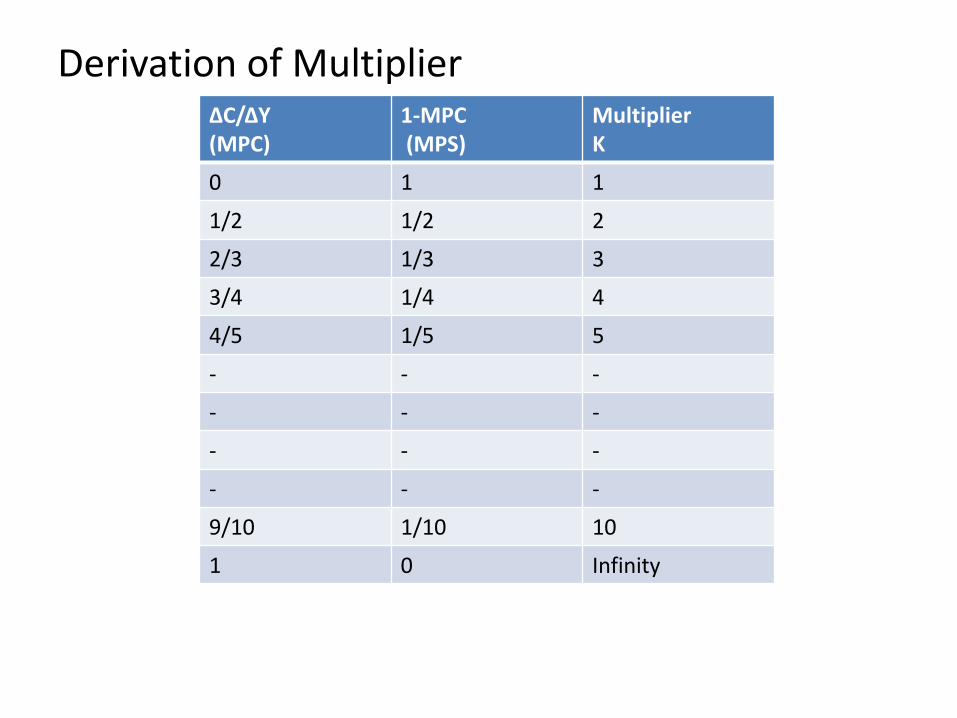
Derivation of Multiplier
ΔC/ΔY (MPC)
1-MPC (MPS)
Multiplier K
0 1 1
1/2 1/2 2
2/3 1/3 3
3/4 1/4 4
4/5 1/5 5
- - -
- - -
- - -
- - -
9/10 1/10 10
1 0 Infinity

When MPC is zero, multiplier is one and induced consumption expenditure is zero. In this case, since nothing is spent out of the extra income from the initial investment, change in investment has a zero multiplier effect on aggregate income. On the other hand, if MPC is one, entire increase in income is spent on consumption. Since MPC is always positive but less than one, multiplier will vary between one and infinity. Thus, the multiplier depends on size of the marginal propensity to consume. Higher the MPC, higher will be the multiplier and vice versa.
Working of Multiplier Multiplier works both forward and backward. In
the forward working of multiplier, an increase in investment leads to an increase in income. This will be explained in the following table

Forward working of Multiplier (Rs. in Million)
Period I Y C
1 10 10 5
2 5 2.50
3 2.50 1.25
4 1.25 0.63
5 0.63 0.32
- - - -
- - - -
Finally 10 20 10

A sum of Rs. 10 million is newly invested in the economy. Those people employed in investment goods industries receive an income of Rs. 10 million and spent a part of their income on consumption goods.If MPC is ½ then Rs. 5 million will be used for buying consumption goods. Now the consumption goods industries get an income of Rs. 5 million to pay the rewards to factors of production in the form of rent, wages, and profits. The recipients of this Rs. 5 million will spend Rs. 2.5 million on consumption. This process will continue till the total income generated increases to Rs. 20 million.
The process of income generation due to an increase in investment is explained with the following diagram.
Aggregate supply curve is represented in the form of a 450 line. Aggregate demand curve, C + I, intersects the 450 line at E. The equilibrium level of income is OY. When investment increases, aggregate demand curve shifts upwards to C + I1 which intersects the aggregate supply curve at E1. The level of income increases to OY1.
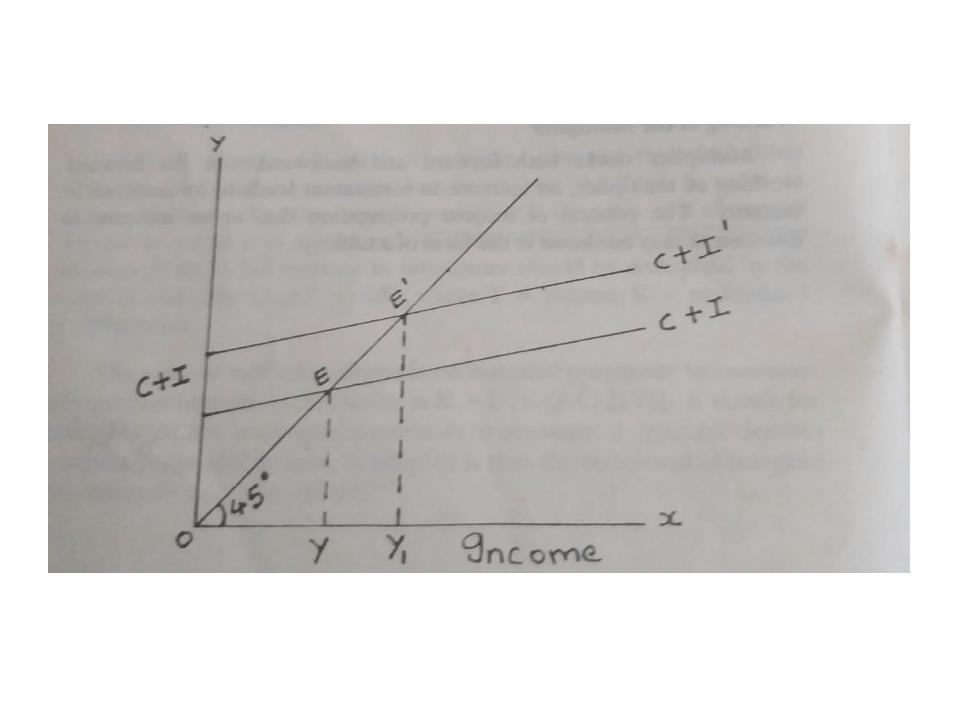
Backward operation of multiplier shows a fall in income due to a reduction in investment. When investment falls by Rs. 10 million, then income will decrease by Rs. 20 million, if MPC is half and multiplier is two. Backward operation of multiplier can be shown in the following diagram.
Aggregate demand curve C + I intersects the 450 line (aggregate supply curve) at E. The equilibrium level of income is OY. Now, when investment decreases, C + I shifts downwards to C+ I1 and income decreases from OY to OY1. Higher the MPC, lower will be the MPS and the effect of a change in investment on income will be larger and vice-versa.

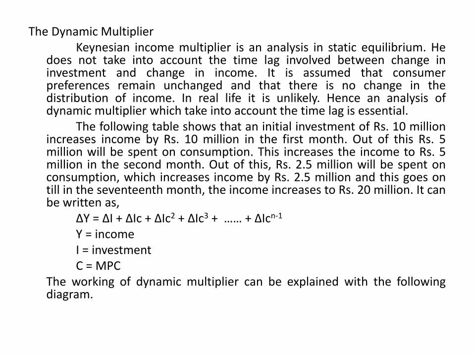
The Dynamic Multiplier Keynesian income multiplier is an analysis in static equilibrium. He
does not take into account the time lag involved between change in investment and change in income. It is assumed that consumer preferences remain unchanged and that there is no change in the distribution of income. In real life it is unlikely. Hence an analysis of dynamic multiplier which take into account the time lag is essential.
The following table shows that an initial investment of Rs. 10 million increases income by Rs. 10 million in the first month. Out of this Rs. 5 million will be spent on consumption. This increases the income to Rs. 5 million in the second month. Out of this, Rs. 2.5 million will be spent on consumption, which increases income by Rs. 2.5 million and this goes on till in the seventeenth month, the income increases to Rs. 20 million. It can be written as,
ΔY = ΔI + ΔIc + ΔIc2 + ΔIc3 + …… + ΔIcn-1
Y = income I = investment C = MPC The working of dynamic multiplier can be explained with the following
diagram.
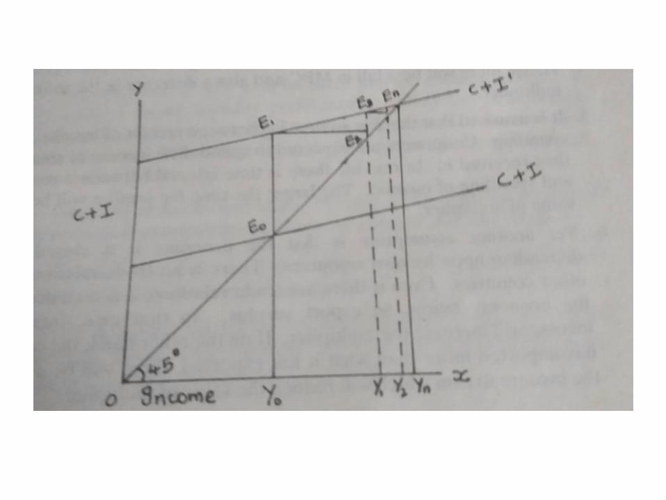
450 line is the aggregate supply curve. C + I represents aggregate demand curve. When aggregate demand and aggregate supply are equal, equilibrium takes at E0 with an equilibrium level of income of OY0. When investment increases, C + I curve shifts upward to C + I1. Now aggregate demand is greater than aggregate supply leading to an increase in income from Y0 to Y1. At this level of income also, aggregate demand exceeds aggregate supply. This will again increase income to OY2. This process will continue till aggregate demand is equal to aggregate supply at Yn level of income.
Assumptions Keynes’ multiplier will operate successfully only under certain assumptions. 1. The investment is kept in a continuous stream. 2. The rise in investment in one sector should not be offset by a fall in investment in
another sector. 3. There is no drastic changes in fiscal policy. 4. There are plenty of consumer goods to facilitate consumption. 5. There is no time lag between receipt of income and spending. 6. Economy is closed one, there is no trade relation with other countries. 7. Value of multiplier depends on the full employment ceiling. 8. There is surplus capacity in consumer goods industries. 9. The economy is industrialized one. 10. Prices are constant 11. Availability of factors of production and other resources with in the economy. 12. Changes occur only in autonomous investment and induced investment is abscent. 13. The accelerator effect on consumption is ignored. 14. Consumption is a function of current income.
Leakages of Multiplier Leakages refer to the diversions from income stream which weaken the
multiplier effect. Leakages may take any form. It is useful to know how the initial investment may leak out of the income stream.
1. Savings constitute an important leakage. Higher the propensity to save lower will be the value of multiplier.
2. Accumulation of idle cash: If people have a strog liquidity preference to satisfy transaction, precautionary, and speculative motives, they will accumulate inactive cash balances.
3. Purchase of stocks and shares by the people from the increased income reduces consumption and hence the value of multiplier falls.
4. If people use a part of the increased income to repay debts to banks, then multiplier process will be checked.
5. Price inflation also affects the working of multiplier. When price increases, a part of the increased income is absorbed by such rise in price leading to a fall in consumption and income.
6. In an open economy, there is always a possibility that a part of the income may leak out of the domestic income stream, if a part of the increased income is used for buying imported goods.. If imports exceed exports there is net deficit in foreign trade and this deficit becomes a leakage.
7. Taxation will reduce consumption and it is an important leakage. 8. If the increased demand for consumption goods is met from the existing stock of
consumption goods, then multiplier will not work.

Criticisms 1. Prof. Haberler has criticised Keynes’ Multiplier as tautological. It is mere
a truism. According to Hansen, it is mere arithmetic multiplier and not a true behaviour multiplier.
2. It is an instantaneous process without time lag. 3. Prof. Hazlitt considers multiplier as a strange concept about which the
Keynesian have made unnecessary fuss. 4. Multiplier analyses only the effect of investment on income but does not
take into account the effect of consumption on investment. 5. Keynes has given too much importance to consumption. 6. Keynes established a linear relationship between consumption and
income. But the relationship between the two is non-linear. Importance 1. Multiplier brings out the importance of investment. 2. It explains different phases of trade cycle. 3. Multiplier process brings out the equality between savings and
investment. 4. It helps in formulating economic policies in order to achieve full
employment and to control trade cycle.

Acceleration The principle of acceleration is important to economic
analysis. It is older than multiplier, and is generally associated with American economist J.M.Clerk. But T.N.Carver was the first economis to analyse the relationship between consumption and investment.. Later on, it was further developed by Hicks, Samuelson and Harrod. Keynes completely ignored it and hence accelerator is not Keynesian concept.
Accelerator shows the effect of a change in consumption on investment. Symbolically, it can be written as
β = ΔI / ΔC where β is accelerator, ΔI is change in investment and ΔC is change in consumption.Demand for consumer goods leads to an increase in demand for capital goods. The principle of acceleration may be shown in the following diagram.


SS is the savings curve and I1, I2 and I3 are autonomous investment curves. The dotted I0 and I1 are induced investment. Savings and investments are equal at point E and the equilibrium level of income is Y0. When investment increases from I1 to I3 income increases from Y0 to Y2. If the increase in investment is autonomous, then the entire increase in income would be due to multiplier effect. But the increase in investment from I to I2 is is autonomous and therefore, Y0Y1 portion of the increase in income is due to multiplier effect. The remaining portion of the increase in income (Y1Y2) is due to acceleration effect. Thus the total multiplier and accelerator effect on income is measured by Y0 Y2. (Y0Y1 due to multiplier effect and Y1Y2 is due to accelerator effect).
Assumption 1. The acceleration principle is based on the constant capital output ratio. 2. It also assumes easy availability of resources. 3. There is absence of excess capacity. 4. Increase in demand is assumed to be permanent. 5. There is elastic supply of credit and capital. 6. It assumes an increase in output leads to a rise in investment.
Limitations 1. It assumes constant capital output ratio. In reality it does not constant, because of
inventions and improvements in techniques of production. 2. It is based on the assumption of easy availability of resources. This is possible only before
full employment. But after full employment, as all the resources are full employed, production can not increased in capital goods industries, this limits the operation of accelerator.
3. It is assumed that there is no excess capacity in plants. If there is excess capacity, an increase in demand may be met by using the idle capacity. Therefore, there will not be any increase in the demand for capital goods. Hence accelerator cannot work.
4. The principle of acceleration will work only if the increased demand is permanent. If the increased demand is temporary, then there will not be any increase in demand for capital goods.
5. Accelerator works only when credit is available easily and in adequate quantities. If credit is not available or if the rate of interest is very high, then investment will fall and accelerator will not work fully.
6. Investment decisions are influenced by changes in stock market, political conditions, economic changes etc. Accelerator neglects the role of expectations in decision making.
Significance of Accelerator 1. The principle of acceleration clearly explains the process of income generation. 2. It helps in understanding the nature and causes of the violent fluctuations in income and
employment. 3. It also shows the turning points of trade cycle particularly upper turning point better than
lower turning point.
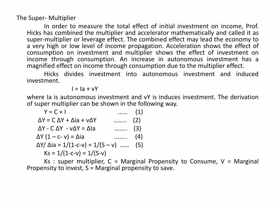
The Super- Multiplier In order to measure the total effect of initial investment on income, Prof.
Hicks has combined the multiplier and accelerator mathematically and called it as super-multiplier or leverage effect. The combined effect may lead the economy to a very high or low level of income propagation. Acceleration shows the effect of consumption on investment and multiplier shows the effect of investment on income through consumption. An increase in autonomous investment has a magnified effect on income through consumption due to the multiplier effect.
Hicks divides investment into autonomous investment and induced investment.
I = Ia + vY where Ia is autonomous investment and vY is induces investment. The derivation
of super multiplier can be shown in the following way. Y = C + I …… (1) ΔY = C ΔY + Δia + vΔY …….. (2) ΔY - C ΔY - vΔY = ΔIa …….. (3) ΔY (1 – c- v) = Δia …….. (4) ΔY/ Δia = 1/(1-c-v) = 1/(S – v) …… (5) Ks = 1/(1-c-v) = 1/(S-v) Ks : super multiplier, C = Marginal Propensity to Consume, V = Marginal
Propensity to invest, S = Marginal propensity to save.

The combined working of multiplier and accelerator can be explained by assuming the
marginal propensity to consume to be 0.5 and marginal propensity to invest as 0.3. Autonomous investment increases by Rs. 100 crores. If the value of super-multiplier is 10, then income will increase to Rs. 1000 crores.
Multiplier-Acceleration interaction (Rs. in crores)
Period Initial Investment
Induced consumption C = 0.5
Induced investment V = 0.3
Increase in income ΔY = C+V
Total increase in income
t + 0 0 0.00 0.00 0.00 0.00
t + 1 100 - - 100.00 100.00
T + 2 100 50.00 30.00 80.00 180.00
T + 3 100 40.00 24.00 64.00 244.00
T + 4 100 32.00 19.20 51.20 295.20
T + 5 100 25.60 15.36 40.90 336.16
- - - - - -
T + n 100 0.00 0.00 0.00 1000.00
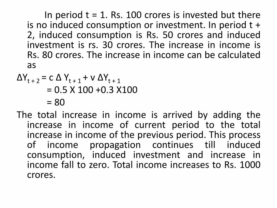
In period t = 1. Rs. 100 crores is invested but there is no induced consumption or investment. In period t + 2, induced consumption is Rs. 50 crores and induced investment is rs. 30 crores. The increase in income is Rs. 80 crores. The increase in income can be calculated as
ΔYt + 2 = c Δ Yt + 1 + v ΔYt + 1
= 0.5 X 100 +0.3 X100 = 80 The total increase in income is arrived by adding the
increase in income of current period to the total increase in income of the previous period. This process of income propagation continues till induced consumption, induced investment and increase in income fall to zero. Total income increases to Rs. 1000 crores.
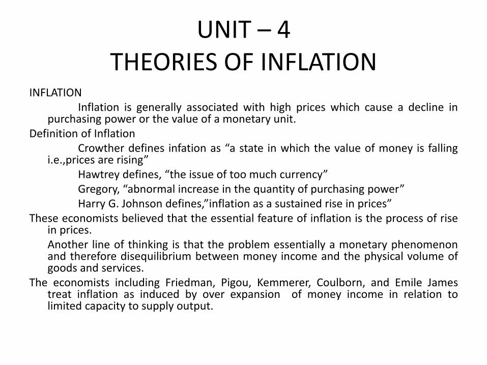
UNIT – 4 THEORIES OF INFLATION
INFLATION Inflation is generally associated with high prices which cause a decline in
purchasing power or the value of a monetary unit. Definition of Inflation Crowther defines infation as “a state in which the value of money is falling
i.e.,prices are rising” Hawtrey defines, “the issue of too much currency” Gregory, “abnormal increase in the quantity of purchasing power” Harry G. Johnson defines,”inflation as a sustained rise in prices” These economists believed that the essential feature of inflation is the process of rise
in prices. Another line of thinking is that the problem essentially a monetary phenomenon
and therefore disequilibrium between money income and the physical volume of goods and services.
The economists including Friedman, Pigou, Kemmerer, Coulborn, and Emile James treat inflation as induced by over expansion of money income in relation to limited capacity to supply output.

Inflationary Gap The inflationary gap is defined by Keynes as an excess of planned expenditure over the
available output at pre-inflation of base price. According to Lipsey “the inflationary gap is the amount by which aggregate expenditure would exeed aggregate output at the full employment level of income”. The inflationary gap for the economy as a whole may be defined in the words of Kurihara “as an excess of anticipated expenditure over available output at base prices”.
The concept of inflationary gap can be explained with an example of war time economy which is generally a full employment economy. The value of Gross National Product is
GNP = C + I + G Where, GNP is Gross national product, C is consumption expenditure, I is Private net investment, G is
government expenditure on goods and services. On the supply side, let us assume that the value of gross national product is Rs. 360 crores, if
government takes away output equivalent to Rs. 150 crores for war purposes, then only Rs. 210 crores worth of output is available for civilian consumption. So the actual value of the available output for civilian consumption is Rs. 210 crores.
On the demand side, let us suppose that the gross national income at the existing price level is Rs. 400 crores. Out of this total national income, if the government takes away Rs. 100 crores by way of taxes, then the total disposable income left with the economy is Rs.300 crores. Assuming that the community pays another sum of Rs,30crores by way of saving then the net disposable income would be Rs.270 crores. This is the actual amount available to the community for spending purposes. Thus Rs. 270 crores is the amount to be spent on available output worth of Rs.210 crores, thereby creating an inflationary gap of Rs. 60 crores. This inflationary gap emerged in the economy due to excess of net disposable income over the available output at constant prices.This process is summarised in the form of below table.
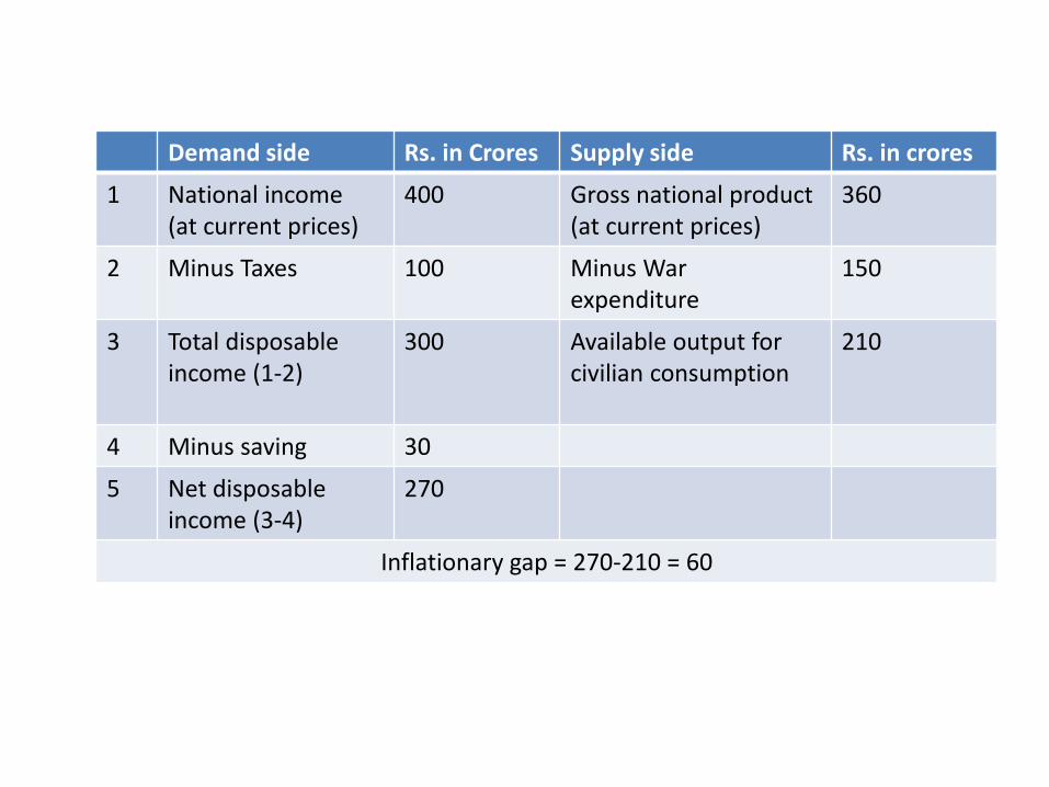
Demand side Rs. in Crores Supply side Rs. in crores
1 National income (at current prices)
400 Gross national product (at current prices)
360
2 Minus Taxes 100 Minus War expenditure
150
3 Total disposable income (1-2)
300 Available output for civilian consumption
210
4 Minus saving 30
5 Net disposable income (3-4)
270
Inflationary gap = 270-210 = 60

From the above table it is clear that there is an inflationary gap in a war time economy. The inflationary gap can not be totally removed during the war time. The increasing supply of consumption goods can reduce this gap, and the government can reduce a part of this gap through taxes, public borrowing and induced savings.
Though Keynes concept of inflationary gap is associated with war time economy, such a phenomenon can occur even in a planned economy.
In the planned economy increase in the money income of the community and investment projects with long gestation period create a wide inflationary gap. The inflationary gap analysis can be explained with the help of the following figure.
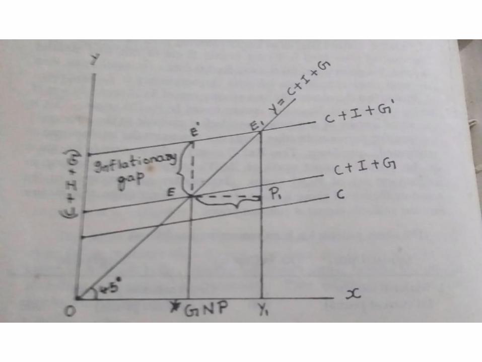

In this figure, X axis represents the gross national product or the real income of the community. Y axis shows the total anticipated expenditure of the economy which is indicated by C + I + G function. The 450 line OE is the equilibrium line indicating that the economy is in equilibrium when the output of goods and services equals the demand for them. Yf is the full employment level of income at the pre inflation prices which arrived at by the equality of aggregate expenditure curve (C + I + G) curve and the 450 line at point E. The aggregate monetary demand here is shown by the C+I+G curve which is equal to EYf. This EYf is equivalent to the total output of goods and services amounting to OYf. Hence there is no possibility of the emergence of an inflationary gap EYf = OYf
If the government expenditure increases by a certain amount say P1E1, the C + I + G curve shifts to a higher level C+ I + G1, where it intersects the 450 line at E1. Thus the new expenditure function in the economy is C+I+G1. Since OYf is the real income of the economy at the full employment level, it does not increase with the increased government expenditure. Now P1E1 represents the excess of monetary demand over the available output of goods (OYf). Thus P1E1 represents inflationary gap. This inflationary gap can be wiped out only when the aggregate money income increases from Yf to Y1 raising the general level of prices. The increase in money income is wholly due to increase in prices since the aggregate real output is constant at the full employment output Yf. We can find out the new equilibrium aggregate income Y1 in the following way Y1 = Yf + ΔG x multiplier.

There are two main causes of inflation: 1. An increase in effective demand, 2. an increase in production costs. The former gives rise to demand-pull inflation, while the latter leads to cost-push inflation.
Demand-pull inflation demand pull inflation or excess demand inflation is described
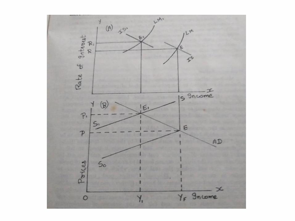
as “too much money chasing too few goods”. The explanation for this can be found in the quantity theory of money. This theory states that prices rise in proportion to the increase in the money supply when the economy is operating at full employment level. As the quantity of money increases, the rate of intyerest will fall and consequently investment will increase. With the situation of full employment equilibrium, if investment demand increases then the aggregate demand for goods and services will exceed their aggregate supply. This equilibrium can be corrected only by way of increase in prices because increase in aggregate supply is not possible at full employment level. The quantity theory version of the demand pull inflation is illustrated in the following figure.


The initial full employment situation is shown by the intersection of IS and LM curves at point E in part (A) of the figure, where R is the interest rate and YF is the full employment level of income. Now with the increase in the quantity of money, the LM curve shifts to LM1 and intersects the IS curve at E1. As a result the equilibrium level of income rises to Y1 and the rate of interest is lowered to R1. as the aggregate supply is assumed to be fixed, there is no change in the position of the IS curve.
Consequently, the aggregate demand rises which shifts the D curve to D1 and thus excess demand is created equivalent to EE1 (=YF Y1) in part B figure. This rise in the price level reduces the real value of the money supply so that the LM1 curve shifts to LM. In this demand pull inflation, if the money supply increases by 10%, the price level also goes up exactly by 10%. Hence the further expansion of production comes to an end.

Cost-Push inflation Cost-push inflation or new inflation is mainly caused by wage push
and profit push to prices. It is due to wage increase enforced by unions, profit increase by employers and sometimes imposition of heavy commodity taxes.
The increase in wages may be caused by powerful trade unions. They press employers to grant wage increases, considerably in excess of increases in the productivity of labour, thereby raising the cost of production of commodities. This attempt on the part of trade unions to push up the wages invariably causes cost inflation in the economy. Secondly employers raise of their products to push up their profit margins. If the prices of products in one industry rise, it raises the production cost in other industries because the output of industry may serve as the input of another industry. Ultimately cost of living will increase leading to increase in wage rate. In this way the wage cost spiral continues thereby leading to cost-push or wage push inflation. Again the government may impose heavy taxes on different goods and producers can easily pass on these taxes to the consumers in the shape of higher prices. This invariably causes cost inflation in the economy.
The cost-push inflation can be explained with the following figure.

In the figure B aggregate demand curve intersects original aggregate supply curve S0 ES at full employment level OYF. When there is an upward shift in the aggregate supply curve to S1ES due to rise in wages, price level rises from OP to OP1. Consequently the equilibrium position shifts from E to E1 reflecting rise in the price level from P to P1 and fall in output, employment and income from YF to Y1 level. Thus in pure cost push inflation the rise in price level is accompanied with rising unemployment. Now consider the upper part of the figure A. As the price level rises, the LM curve shifts to the left to LM1 position because with the increase in the price level to P1 the real value of the money supply falls. Similarly, the IS curve shifts to the left to IS1 position because with the increase in the price level the demand for consumer goods falls due to the Pigou effect. Accordingly, the equilibrium position of the economy shifts from E to E1 where the interest rate increases from R to R1 and the output, employment and income levels fall from the full employment level of YF to Y1. The system is now in equilibrium at Y1, less than full employment level of income and the unemployment equal to the gap Y1 – YF exists. If the government or monetary authority is committed to maintain full employment, the price should increase much more than this.
l

Effects of Inflation
Mild inflation caused by an expansion of money supply may actually be good for the economy particularly when there are unemployed resources in the country. But after the full employment of productive resources, any expansion of money supply is bound to result in continuous inflation which shakes the foundation of the political and economic stability of the economy.
Thus inflation has good and bad effects on the economy. The effects of inflation explained under two heads as follows.
Effects on Production
1. Hyper inflation discourages savings on the part of the public. With reduced savings and capital accumulation, the investment will suffer a serious set-back which may have an adverse effect on the volume of production in the country.
2. It may discourage entrepreneurs and businessmen from taking business risk in production.
3. It results in a serious depreciation of the value of money.
4. It may drive out the foreign capital already exists in the country.
5. It may lead to a serious deterioration in the quality of goods produced in the economy
6. Diversion of productive resources from the essential goods to luxury goods, creating further shortages of consumer goods.
7. It leads to holding of essential goods both by the traders as well as by the consumers.
8. It disrupts the smooth working of the price mechanism, thereby creating all-round confusion in the economy
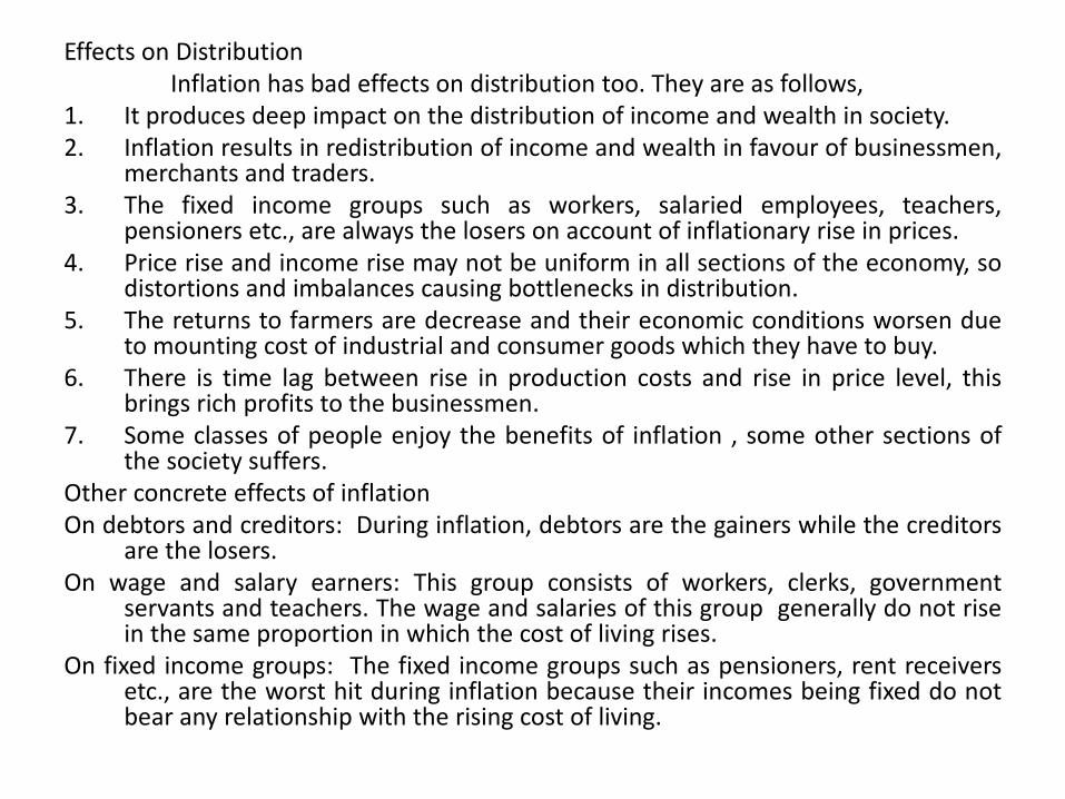
Effects on Distribution Inflation has bad effects on distribution too. They are as follows, 1. It produces deep impact on the distribution of income and wealth in society. 2. Inflation results in redistribution of income and wealth in favour of businessmen,
merchants and traders. 3. The fixed income groups such as workers, salaried employees, teachers,
pensioners etc., are always the losers on account of inflationary rise in prices. 4. Price rise and income rise may not be uniform in all sections of the economy, so
distortions and imbalances causing bottlenecks in distribution. 5. The returns to farmers are decrease and their economic conditions worsen due
to mounting cost of industrial and consumer goods which they have to buy. 6. There is time lag between rise in production costs and rise in price level, this
brings rich profits to the businessmen. 7. Some classes of people enjoy the benefits of inflation , some other sections of
the society suffers. Other concrete effects of inflation On debtors and creditors: During inflation, debtors are the gainers while the creditors
are the losers. On wage and salary earners: This group consists of workers, clerks, government
servants and teachers. The wage and salaries of this group generally do not rise in the same proportion in which the cost of living rises.
On fixed income groups: The fixed income groups such as pensioners, rent receivers etc., are the worst hit during inflation because their incomes being fixed do not bear any relationship with the rising cost of living.
On investors: Investors are of two types (1) investors in equities and (2) investors in fixed interest-earing bonds and debentures. The equity holders stand to gain because the return on equities varies with the rising prices. More devidends available to them, however fixed interest –earning bonds and debentures have much to lose during inflation.
On farmers: Farmers are divided into three broad categories (1) non-cultivating landlords (2) peasant proprietors and (3) farm labourers. Landlords are the losers during nflation since the rents are fixed by contracts over a long period of time. The peasant proprietors gain substantially because they bring considerably surplus to the market when prices move in the upward direction. The farm labourers are very badly affected by the rise in prices since these people receive very low fixed income.
Social, moral and political effects: Inflation is socially unjust and inequitable for society because it redistributes income and wealth in favour of well-off. This leads to social conflicts in society. The general morality of the people in the country also suffers a serious decline with the resulting all-round corruption in the country. The political agitations and protests are launched by the public.
Control of inflation The measures against inflation can be classified into three broad categories.
They are (1) Monetary measures (2) Fiscal measures (3) other measures.
Monetary measures Monetary measures can help in reducing the pressure of demand.
These measures are adopted by the central bank of the country to reduce inflation through reduction of money supply and credit.
Increased re-discount rates: To curb inflation, the central bank increases the rediscount rates. An increase in rediscount rates leads to an increase in the interest rates charged by commercial banks which tends to discourage borrowings by businessmen and consumers from banks and thus discourages excessive activity in the economy. Again an increase in the rate of interest may make saving more attractive than before so that some people will be tempted to consume less of their income than before.
Sale government securities in the open market: If the central bank wants to reduce the credit creation by commercial banks, it will sell government securities to the public or the banks themselves. Either way, the result will be that the amount of cash with the banks will diminish and this will force them to reduce the supply of credit.
Higher reserve requirements: An increase in reserve requirements of the member-banks also serves as an anti-inflationary weapon. If the central bank raises the legal reserve requirements from 20% to 25% then the member banks required to keep large reserves with the central bank, their power to create credit shall become limited.
Consumer credit control: This devise is introduced to curb excess spending on the part of consumers. During an inflationary boom facilities for installment buying of durable consumer goods are reduced to reduce excessive spending.
Higher margin requirements: This is a method of selective credit control. The higher the margin requirement, the lower the amount of the loan that the borrower can obtain from the bank.
Fiscal measures By adopting suitable measures in public expenditure, taxation, public borrowing,
debt management and over valuation the government can reduce inflation. Government Expenditure: During the time of inflation, the basic cause of inflationary
pressures is the excessive aggregate spending. Therefore, prper public expenditure policy must attempt to reduce the government spending through the abandonment of the some of the schemes and the postponement of some others.
Taxation: An increase in taxes tends to reduce private spending. The rates of existing taxes should be steeply increased while new taxes should be imposed on commodities and services so as to leave less money supply with the public to spend.
Public borrowing: The object of public borrowing is to take away from the public excess purchasing power in view of the limited supply of goods and services. Public borrowing may be voluntary or compulsory. Voluntary borrowing does not bring to the government sufficient amounts to have really effective impact on the inflationary pressurews. It thus becomes essential to resort to compulsory borrowing from the public.
Debt management: At the time of inflation, the government may be faced with adeficit budget. The government can repay bank-held debt by sale of bank-ineligible bonds to non-bank investors. This will have the effect of taking away spendable money from the public and control inflation.
Over valuation: An over valuation of domestic currency in terms of foreign currencies will also serve as an anti-inflationary measure. This method will discourage exports and encourage imports and thereby increased availability of goods and services in the domestic market.
Other measures
Other measures like expansion of output, wage policy, price control and rationing can be used to supplement the monetary-fiscal measures undertaken to contain inflationary pressures.
Expansion of output: Inflationary gap arises partly due to the inadequacy of output. A reallocation of productive resources is suggested to step up the ouput of essential consumer goods. Efforts should be made by the authorities to keep the factor prices in check because factor prices may rise up with an increase of output thus adding more fuel to the inflationary fire.
Wage policy: Wages cannot be left free to chase price upward. If wages increases it will increase the productivity of the workers.
Price control and rationing: The object of price control is to lay down the upper limit beyond which the price of a particular commodity would not be allowed to rise. Two conditions have to be satisfied for the successful functioning of price control. Firstly the government should have under its control adequate stock of the commodity concerned. Secondly the demand for the concerned commodity should be controlled through rationing.

UNIT – 5 GENERAL EQUILIBRIUM OF PRODUCT AND
MONEY MARKET Introduction
The concept of general equilibrium is used to explain the situation which there is a simultaneous equilibrium in both goods market and money market, The keynesian one sector model deals with the equilibrium in the goods market and it does not deal with the money market equilibrium.
Goods market equilibrium is defined by an equality between savings and investment. Savings is a direct function of income. S = f(Y). Investment is an inverse function of rate of interest. I = f(r). IS schedule represents the combination of interest rate and income level where savings and investment equilibrium takes place. At that point, the product market is in equilibrium. This is also known as real equilibrium at which I = S.
Money market equilibrium is defined by an equality between demand and supply of money. In equilibrium L = M, where L denotes demand for money and M denotes supply of money. The total demand for money is divided into Transaction and Precautionary (L1) demand for money (which is a function of income) and speculative (L2) demand for money and it is inverse function of interest.
In equilibrium L = M, there is an interaction between money market and goods market. The study of the interaction between the two markets forms the core of general equilibrium model.
` A.H. Hansen and J.R.Hicks brought about synthesis between goods market and money market. In order to analyse the general equilibrium analysis, the economy it can be divided into goods market and money market.
Commodity market Equilibrium – IS IS curve is the locus of all interest rates and income
levels at which commodity market is in equilibrium. At that point, the demand foe and supply of commodities are equal. In other words, equilibrium occurs at the point at which saving and investment are equal. Derivation of IS can be shown in the following figure.


In the first quadrant, investment demand schedule is shown. Rate of interest is measured in Y axis and level of investment is shown in the X axis. It shows the inverse relation between the two that is when rate of interest is high, level of investment is low and vice-versa.
Saving investment equality is shown in second quadrant. Since saving is always equal to investment, this curve is a straight line or 450 line from the origin.
In third quadrant, saving schedule is plotted. Here it is assumed that the level of saving is zero at an income level of Rs.100 crores and the marginal propensity to save is 0.5.
The fourth quadrant depicts the product market equilibrium. The derivation of IS or product market equilibrium can be explained by taking 3 percent as the rate of interest. At that rate of interest the level of investment is Rs. 50 crores which is shown in the first quadrant. When investment is Rs,50 crores savings may also be 50 crores which shown in the second quadrant. In quadradt three, the saving function indicates that rs, 50 crores can be saved only at an income level of Rs. 200 crores. In the fourth quadrant, at one point equilibrium can be obtained that is when the rate of interest is 3%, the level of income which will equate saving and investment is Rs. 200 crores.
If the rate of interest increases to 4%, investment falls to Rs.25 crores. Saving will also be Rs. 25 crores and the level of income at which rs. 25 crores can be saved is Rs. 150 crores. If the rate of interest falls to 2%, investment increases to Rs.75 crores, and the equilibrium level of income is Rs.250 crores. By joining the different points of equilibrium rates of interest and levels of income, IS curve can be obtained.
Money Market Equilibrium – LM Monetary equilibrium or derivation of LM curve
can also be shown in the same way. LM is the locus of combinations of interest rate and real income levels at which the supply of money equals the demand for money, which is shown in the following figure
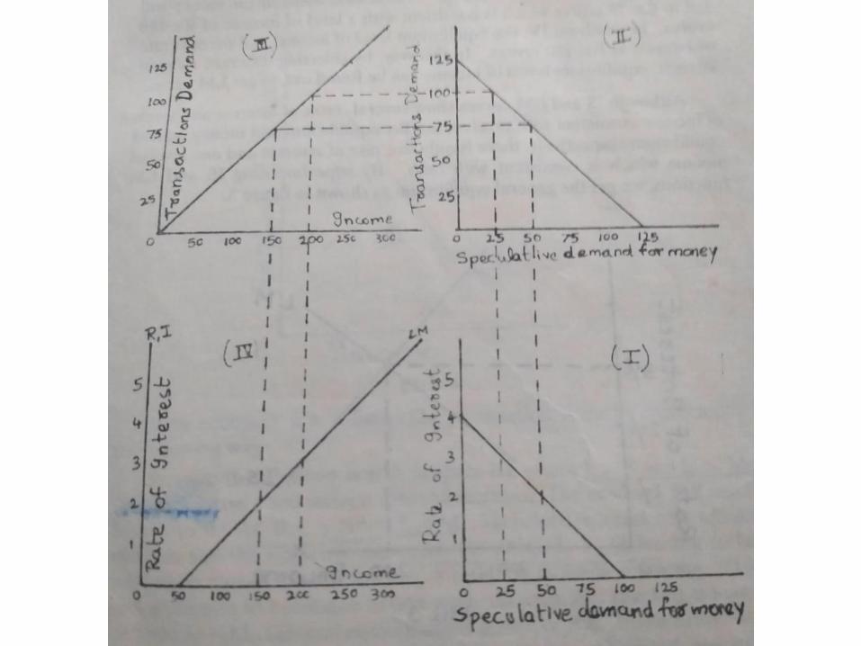
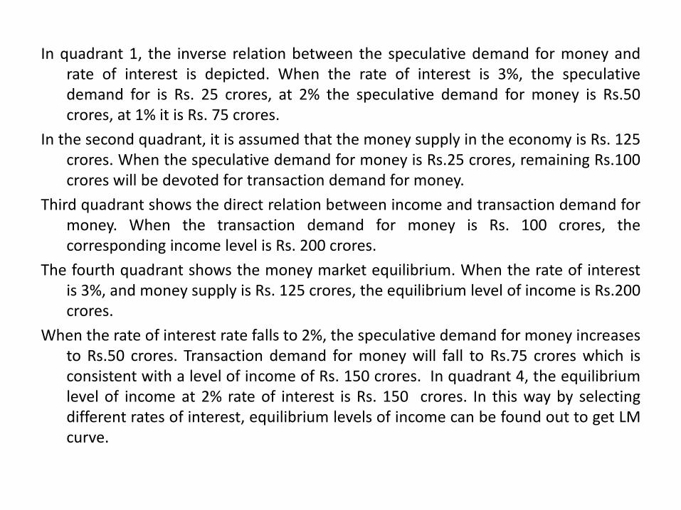
In quadrant 1, the inverse relation between the speculative demand for money and rate of interest is depicted. When the rate of interest is 3%, the speculative demand for is Rs. 25 crores, at 2% the speculative demand for money is Rs.50 crores, at 1% it is Rs. 75 crores.
In the second quadrant, it is assumed that the money supply in the economy is Rs. 125 crores. When the speculative demand for money is Rs.25 crores, remaining Rs.100 crores will be devoted for transaction demand for money.
Third quadrant shows the direct relation between income and transaction demand for money. When the transaction demand for money is Rs. 100 crores, the corresponding income level is Rs. 200 crores.
The fourth quadrant shows the money market equilibrium. When the rate of interest is 3%, and money supply is Rs. 125 crores, the equilibrium level of income is Rs.200 crores.
When the rate of interest rate falls to 2%, the speculative demand for money increases to Rs.50 crores. Transaction demand for money will fall to Rs.75 crores which is consistent with a level of income of Rs. 150 crores. In quadrant 4, the equilibrium level of income at 2% rate of interest is Rs. 150 crores. In this way by selecting different rates of interest, equilibrium levels of income can be found out to get LM curve.

Intersection of IS and LM curves
Although IS and LM curves show several rates of interest and levels of income consistent with goods market equilibrium and money market equilibrium respectively., there is only one rate of interest and one level of income which is consistent with both. By Superimposing IS and LM functions, we get the general equilibrium as shown in the following figure.
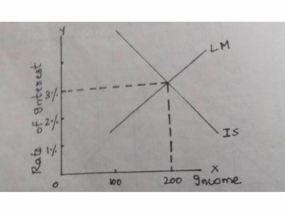

The intersection of IS and LM takes place at 3% rate of interest and Rs.200 crores of income level. At this rate of interest and level of income, the level of investment is Rs.100 crores. There is general equilibrium at 3% rate of interest and Rs. 200 crores level of income. Thus, there is only one combination of intersect at which both I = S and L = M. At all other combinations of income and rate of interest, there is disequilibrium in either goods market or money market or both.

Shift in IS Function IS function may shift due to a reduction in saving. It
may be due to an increase in consumption due to an expectation of a rise in price. IS function may also shift due to an increase in investment which is caused by an expectation of higher profits or innovation or rise in demand. The shift of IS curve with the given LM and consequent change in equilibrium shown in the following figure.
IS curve shifts from IS to IS1 due to a reduction in saving or increase in investment. Equilibrium changes from E to E1 leading to an increase in income and rate of interest. When investment falls or saving increases, IS function will shift to the left and equilibrium is established at a lower income level and interest rate.
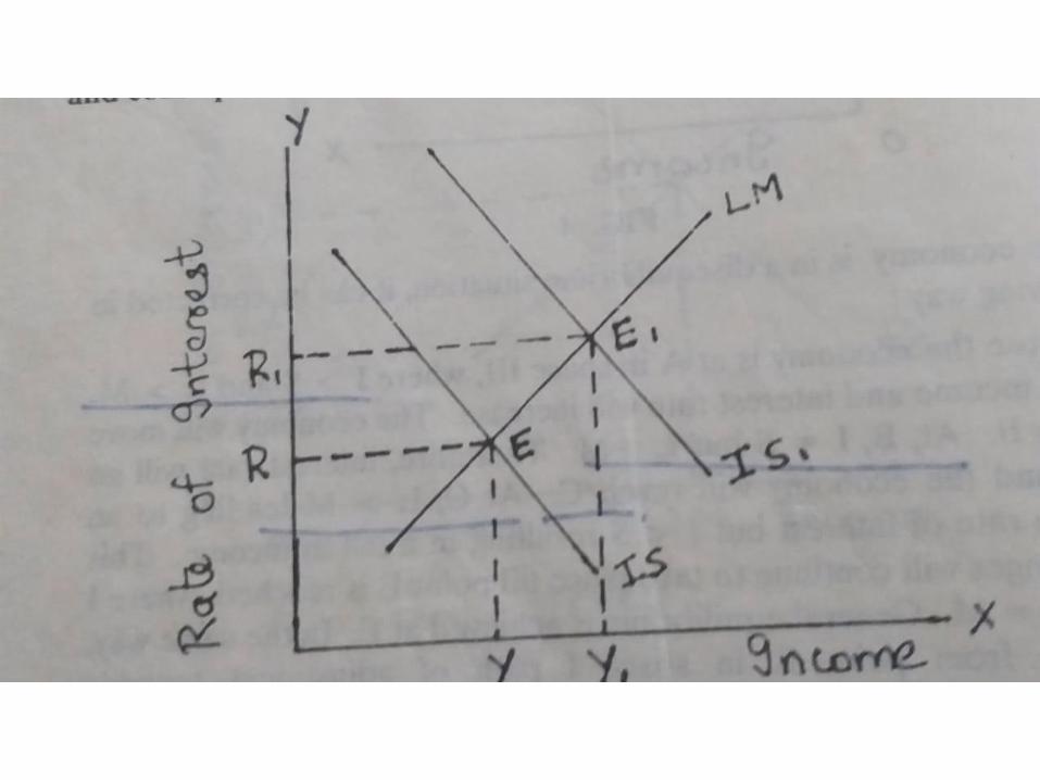
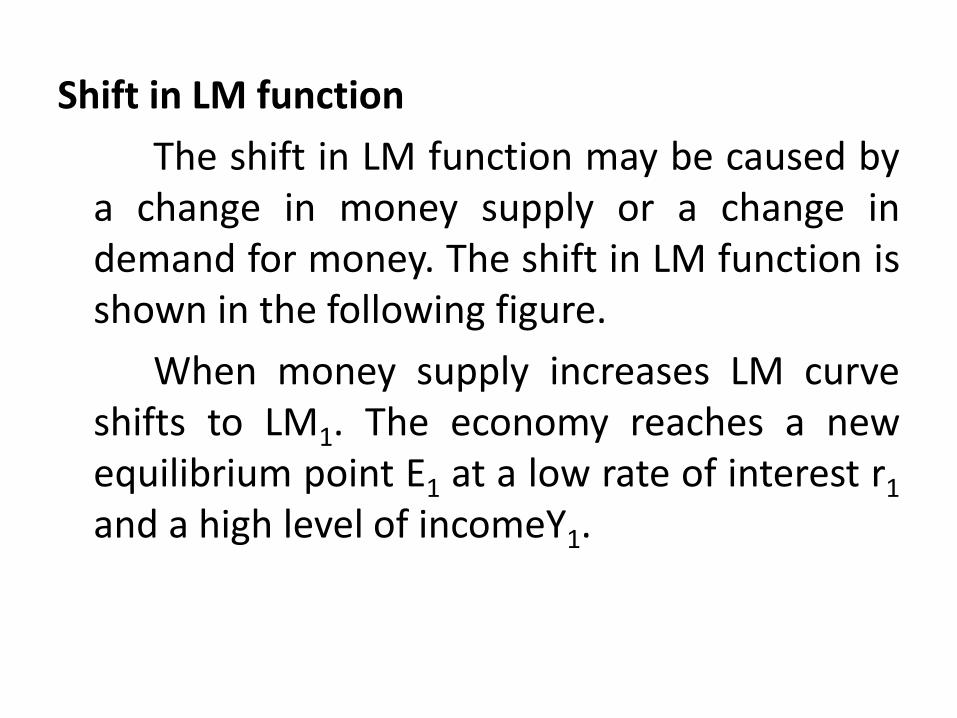
Shift in LM function
The shift in LM function may be caused by a change in money supply or a change in demand for money. The shift in LM function is shown in the following figure.
When money supply increases LM curve shifts to LM1. The economy reaches a new equilibrium point E1 at a low rate of interest r1 and a high level of incomeY1.


Simultaneous Shifts in IS and LM functions When IS function shifts due to an increase in investment and LM function due to an increase in money supply both the level of income and rate of interest change. The effect of a simultaneous shift in IS and LM on income and rate of interest is illustrated in the following figure.
An increase in investment shifts IS curve to IS1 and the increase in money supply shifts LM curve to LM1. Equilibrium changes from E to E1. Rate of interest remains at the same level but the level of income increases from OY to OY1. If LM remains the same IS alone changes, equilibrium changes to E2. Both interest rate and level of income increase.


