Macroeconomic Data Transformations Matter * Philippe Goulet Coulombe 1† Maxime Leroux 2 Dalibor Stevanovic 2‡ Stéphane Surprenant 2 1 University of Pennsylvania 2 Université du Québec à Montréal This version: March 9, 2021 Abstract In a low-dimensional linear regression setup, considering linear transformations/combinations of predictors does not alter predictions. However, when the forecasting technology either uses shrinkage or is nonlinear, it does. This is precisely the fabric of the machine learning (ML) macroeconomic forecasting environment. Pre-processing of the data translates to an alter- ation of the regularization – explicit or implicit – embedded in ML algorithms. We review old transformations and propose new ones, then empirically evaluate their merits in a substantial pseudo-out-sample exercise. It is found that traditional factors should almost always be in- cluded as predictors and moving average rotations of the data can provide important gains for various forecasting targets. Also, we note that while predicting directly the average growth rate is equivalent to averaging separate horizon forecasts when using OLS-based techniques, the latter can substantially improve on the former when regularization and/or nonparametric nonlinearities are involved. JEL Classification: C53, C55, E37 Keywords: Machine Learning, Big Data, Forecasting. * We thank the Editor Esther Ruiz, two anonymous referees, and Hugo Couture who provided excellent research assistance. We acknowledge financial support from the Chaire en macroéconomie et prévisions ESG UQAM. † Corresponding Author: [email protected]. Department of Economics, UPenn. ‡ Corresponding Author: [email protected]. Département des sciences économiques, UQAM. 1
Transcript
Macroeconomic Data Transformations Matter*
Philippe Goulet Coulombe1† Maxime Leroux2 Dalibor Stevanovic2‡
Stéphane Surprenant2
1University of Pennsylvania2Université du Québec à Montréal
This version: March 9, 2021
Abstract
In a low-dimensional linear regression setup, considering linear transformations/combinations
of predictors does not alter predictions. However, when the forecasting technology either uses
shrinkage or is nonlinear, it does. This is precisely the fabric of the machine learning (ML)
macroeconomic forecasting environment. Pre-processing of the data translates to an alter-
ation of the regularization – explicit or implicit – embedded in ML algorithms. We review old
transformations and propose new ones, then empirically evaluate their merits in a substantial
pseudo-out-sample exercise. It is found that traditional factors should almost always be in-
cluded as predictors and moving average rotations of the data can provide important gains for
various forecasting targets. Also, we note that while predicting directly the average growth
rate is equivalent to averaging separate horizon forecasts when using OLS-based techniques,
the latter can substantially improve on the former when regularization and/or nonparametric
nonlinearities are involved.
JEL Classification: C53, C55, E37
Keywords: Machine Learning, Big Data, Forecasting.*We thank the Editor Esther Ruiz, two anonymous referees, and Hugo Couture who provided excellent research
assistance. We acknowledge financial support from the Chaire en macroéconomie et prévisions ESG UQAM.†Corresponding Author: [email protected]. Department of Economics, UPenn.‡Corresponding Author: [email protected]. Département des sciences économiques, UQAM.
Following the recent enthusiasm for Machine Learning (ML) methods and widespread avail-
ability of big data, macroeconomic forecasting research gradually evolved further and further
away from the traditional tightly specified OLS regression. Rather, nonparametric non-linearity
and regularization of many forms are slowly taking the center stage, largely because they can
provide sizable forecasting gains when compared with traditional methods (see, among others,
Kim and Swanson (2018); Medeiros et al. (2019); Goulet Coulombe et al. (2019); Goulet Coulombe
(2020a)), even during the Covid-19 episode (Goulet Coulombe et al., 2021). In such environments,
different linear transformations of the informational set X can change the prediction and taking
first differences may not be the optimal transformation for many predictors, despite the fact that
it guarantees viable frequentist inference. For instance, in penalized regression problems – like
Lasso or Ridge –, different rotations of X imply different priors on β in the original regressor
space. Moreover, in tree-based models algorithms, since the problem of inverting a near sin-
gular matrix X′X simply does not happen, making the use of more persistent (and potentially
highly cross-correlated regressors) much less harmful. In sum, in the ML macro forecasting en-
vironment, traditional data transformations – such as those designed to enforce stationarity (Mc-
Cracken and Ng, 2016) – may leave some forecasting gains on the table. To provide guidance for
the growing number of researchers and practitioners in the field, we conduct an extensive pseudo-
out-of-sample forecasting exercise to evaluate the virtues of standard and newly proposed data
transformations.
From the ML perspective, it is often suggested that a "feature engineering" step may improve
algorithms’ performance (Kuhn and Johnson, 2019). This is especially true of Random Forests
(RF) and Boosted Trees (BT), two regression tree ensembles widely regarded as the most per-
forming off-the-shelf algorithms within the modern ML canon (Hastie et al., 2009). Among other
things, both successfully handle a high-dimensional X by recruiting relevant predictors in a sea of
useless ones. This implies the data scientist leveraging some domain knowledge can create plau-
sibly more salient features out of the original data matrix, and let the algorithm decide whether to
use them or not. Of course, an extremely flexible model, like a neural network with many layers,
could very well create those relevant transformations internally in a data-driven way. Yet, this
idyllic scenario is a dead end when data points are few, regressors are numerous, and a noisy y
serves as a prediction target. This sort of environment, of which macroeconomic forecasting is a
notable example, will often benefit from any prior knowledge one can incorporate in the model.
Since transforming the data transforms the prior, doing so properly by including well-motivated
rotations of X has the power to increase ML performance on such challenging data sets.
Macroeconomic modelers have been thinking about designing successful priors for a long
2
time. There is a wide literature on Bayesian Vector Autoregressions (VAR) starting with Doan
et al. (1984). Even earlier on, the penalized/restricted estimation of lag polynomials was exten-
sively studied (Almon, 1965; Shiller, 1973). The motivation for both strands of work is the large
ratio of parameters to observations. Forty years later, many more data points are available, but
models have grown in complexity. Consequently, large VARs (Banbura et al., 2010) and MIDAS
regression (Ghysels et al., 2004) still use those tools to regularize over-parametrized models. ML
algorithms, usually allowing for sophisticated functional forms, also critically rely on shrinkage.
However, when it comes to nonlinear nonparametric methods – especially Boosting and Random
Forests – there are no explicit parameters to penalize. Nevertheless, in the case of RF, the ensu-
ing ensemble averaging prediction benefits from ridge-like shrinkage as randomization allows
each feature to contribute to the prediction, albeit in a moderate way (Hastie et al., 2009; Mentch
and Zhou, 2019). Just like rotating regressors changes the prior in a Ridge regression (see discus-
sion in Goulet Coulombe (2020b)), rotating regressors in such algorithms will alter the implicit
shrinkage scheme – i.e., move the prior mean away from the traditional zero. This motivates us
to propose two rotations of X that implicitly implement a more time-series-friendly prior in ML
models: moving average factors (MAF) and moving average rotation of X (MARX). Other than
those motivated above, standard transformations are also being studied. This includes factors
extracted by principal components of X and the inclusion of variables in levels to retrieve low
frequency information.
We are interested in predicting stationary targets through a direct (in opposition to iterated)
forecasting approach. There are at least two ways one can construct direct forecasts of the average
growth rate of a variable over the next h > 1 months – an important quantity for the conduct of
monetary policy and fiscal planning. A popular approach is to forecast the final object of interest
by projecting it directly on the informational set X (e.g., Stock and Watson 2002a). An alterna-
tive is the path average approach where every step until the final horizon is predicted separately.
A potential benefit of fitting the whole path first and then constructing the final target is to al-
low for the selected predictors, the harshness of regularization, and the type of nonlinearities to
fully adapt when different relationships arise among the variables during the path.1 Since those
three modeling elements are wildly nonlinear operations in the original input, averaging the path
before or after ML is performed can produce very different results.
To evaluate the contribution of data transformations for macroeconomic prediction, we con-
duct an extensive pseudo-out-of-sample forecasting experiment (38 years, 10 key monthly macroe-
conomic indicators, 6 horizons) with three linear and two nonlinear ML methods (Elastic Net,
Adaptive Lasso, Linear Boosting, Random Forests, and Boosted Trees), and two standard econo-
metric reference models (autoregressive and factor-augmented autoregression).
1An obvious drawback is that implies estimating and tuning h models rather than one.
3
Main results can be summarized as follows. First, combining non-standard data transforma-
tions, MARX, MAF and Level, minimizes the RMSE for 8 and 9 variables out of 10 when respec-
tively predicting at short horizons 1 and 3-month ahead. They remain resilient at longer horizons
as they are part of best RMSE specifications around 80% of time. Second, their contribution is
magnified when combined with nonlinear ML models – 38 out of 47 cases2 – with an advantage
for Random Forests over Boosted Trees. Both algorithms allow for nonlinearities via tree base
learners and make heavy use of shrinkage via ensemble averaging. This is precisely the algo-
rithmic environment we conjectured could benefit most from non-standard transformations of X.
Third, traditional factors can help tremendously. The overwhelming majority of best information
sets for each target included factors. On that regard, this amounts to a clear takeaway message:
while ML methods can handle the high-dimensional X (both computationally and statistically),
extracting common factors remains straightforward feature engineering that pays off. Fourth,
the path average approach is preferred to the direct counterpart for almost all real activity vari-
ables and at most horizons. Combined with high-dimensional methods that use some form of
regularization improves predictability by as much as 30%.
The rest of the paper is organized as follows. In section 2, we present the ML predictive
framework and detail the data transformations and forecasting models. In section 3, we detail the
forecasting experiment and in section 4 we present main results. Section 5 concludes.
2 Machine Learning Forecasting Framework
Machine learning algorithms offer ways to approximate unknown and potentially compli-
cated functional forms with the objective of minimizing the expected loss of a forecast over h
periods. The focus of the current paper is to construct a feature matrix susceptible to improve the
macroeconomic forecasting performance of off-the-shelf ML algorithms. Let Ht = [H1t, ..., HKt]
for t = 1, ..., T be the vector of variables found in a large macroeconomic dataset and let yt+h be
our target variable that is supposed stationary. The corresponding prediction problem is given by
yt+h = g( fZ(Ht)) + et+h. (1)
To illustrate the data pre-processing point, define Zt ≡ fZ(Ht) as the NZ-dimensional feature
vector, formed by combining several transformations of the variables in Ht.3 The function fZ rep-
resents the data pre-processing and/or featuring engineering whose effects on forecasting perfor-
2There are 47 cases where at least one of these transformations is used.3Obviously, in the context of a pseudo-out-of-sample experiment, feature matrices must be built recursively to
avoid data snooping.
4
mance we seek to investigate. The training problem for fZ = I() is
ming∈G
{T
∑t=1
(yt+h − g (Ht))2 + pen(g; τ)
}. (2)
The function g, chosen as a point in the functional space G, maps transformed inputs into the
transformed targets. pen() is the regularization function whose strength depends on some vec-
tor/scalar hyperparameter(s) τ. Let ◦ denote the function product and g := g ◦ fZ. Clearly,
introducing a general fZ leads to
ming∈G
{T
∑t=1
(yt+h − g ( fZ(Ht)))2 + pen(g; τ)
}↔ min
g∈G
{T
∑t=1
(yt+h − g (Ht))2 + pen( f−1
Z ◦ g; τ)
}
which is, simply, a change of regularization. Now, let g∗( f ∗Z(Ht)) be the "oracle" combination
of best transformation fZ and true function g. Let g( fZ(Ht)) be a functional form and data pre-
processing selected by the practitioner. In addition, denote g(Zt) and yt+h the fitted model and
its forecast. The forecast error can be decomposed as
While the intrinsic error et+h is not shrinkable, the estimation error can be reduced by either
adding more relevant data points or restricting the domain G. The benefits of the latter can be
offset by a corresponding increase of the approximation error. Thus, an optimal fZ is one that
entails a prior that reduces estimation error at a minimal approximation error cost. Additionally,
since most ML algorithms perform variable selection, there is the extra possibility of pooling
different fZ’s together and let the algorithm itself choose the relevant restrictions.4
The marginal impact of the increased domain G has been explicitly studied in Goulet Coulombe
et al. (2019), with Zt being factors extracted from the stationarized version of FRED-MD. The pri-
mary objective of this paper is to study the relevance of the choice of fZ, combined with popular
ML approximators g.5 To evaluate the virtues of standard and newly proposed data transforma-
tions, we conduct a pseudo-out-of-sample (POOS) forecasting experiment using various combi-
nations of fZ’s and g’s.
4More concretely, a factor F is a linear combination of X. If an algorithm pick F rather than creating its owncombination of different elements of X, it is implicitly imposing a restriction.
5There are many recent contributions considering the macroeconomic forecasting problem with econometric andmachine learning methods in a big data environment (Kim and Swanson, 2018; Kotchoni et al., 2019). However, theyare done using the standard stationary version of FRED-MD database. Recently, McCracken and Ng (2020) studiedthe relevance of unit root tests in the choice of stationarity transformation codes for macroeconomic forecasting withfactor models.
5
Finally, a question often overlooked in the forecasting literature is how one should construct
the forecast for average growth/difference of the level variable Yt, which is the popular tar-
get in macroeconomic applications. The usual approach – and also the least computationally
demanding – is that of fitting the model on yt+h = ∑hh′=1 ∆Yt+h′/h directly and using ydirect
t+h as
prediction, where ∆Yt+h′ = Yt+h′ − Yt+h′−1 is the simple growth/difference of the variable of
interest. Another approach, requiring the estimation of h different functions, is the path aver-
age approach where each ∆Yt+h′ is fitted separately and the forecast for yt+h is obtained from
ypath-avgt+h = ∑h
h′=1 ∆Yt+h′/h.
The common wisdom – from OLS – is that such strategies are interchangeable. But the equiv-
alence does not hold when regularization and nonparametric nonlinearities are involved. For
instance, it breaks in the simplest possible departure from OLS, a ridge regression, where
ypath-avgt+h =
1h
h
∑h′=1
Z(Z′Z + λh′ I)−1Z′∆Yt+h′ , (4)
and only if λh′ = λ ∀h′ then
ypath-avgt+h = Z(Z′Z + λI)−1Z′
∑hh′=1 ∆Yt+h′
h= ydirect
t+h . (5)
This setup naturally includes the known equivalence in the OLS case (λh′ = 0 ∀h′). We get even
further from the equivalence with Lasso, Random Forests, and Boosted Trees which all imply the
nonlinear hard-thresholding operation of variable selection – and basis expansion creation for the
last two. With those, we get even further from the equivalence by having a different Z∗h′ ⊂ Z in
each prediction function.
Of course, the path average approach can be rather demanding since it implies h estimation
(and likely cross-validation) problems — with the benefit of providing a whole path rather than
merely yt+h. The second question address then concerns whether those benefits could addition-
ally include forecasting gains. To investigate this and how this choice interacts with the optimal
fZ, we conduct the whole forecasting exercise using both schemes.
2.1 Old News
Firstly, we consider more traditional candidates for fZ.
INCLUDING FACTORS. Common practice in the macroeconomic forecasting literature is to rely
on some variant of the transformations proposed by McCracken and Ng (2016) to obtain a station-
ary Xt out of Ht. Letting X = [Xt]Tt=1 and imposing a linear latent factor structure X = FΛ + ε,
we can estimate F by the principal components of X. The feature matrix of the autoregressive
6
diffusion index (FM hereafter) model of Stock and Watson (2002a,b) can be formed as
where L is the lag operator and yt is the current value of the target. In Goulet Coulombe et al.
(2019), factors were deemed the most reliable shrinkage method for macroeconomic forecasting,
even when considering ML alternatives. Furthermore, the combination of factors (and nothing
else) with nonlinear nonparametric methods is (i) easy, (ii) fast, and (iii) often quite successful.
Point (iii) is further re-enforced by this paper’s results, especially for forecasting inflation, which
contrasts with the results found in Medeiros et al. (2019).
INCLUDING LEVELS. In econometrics, debates on the consequences of unit roots for frequentist
inference have a long history6, just as does the handling of low frequency movements for macroe-
conomic forecasting (Elliott, 2006). Exploiting potential cointegration has been found useful to
improve forecasting accuracy under some conditions (e.g., Christoffersen and Diebold (1998);
Engle and Yoo (1987); Hall et al. (1992)). From the perspective of engineering a feature matrix,
the error correction term could be obtained from a first step regression à la Engle and Granger
(1987) and is just a specific linear combination of existing variables. When it is unclear which
variables should enter the cointegrating vector – or whether there exist any such vector – one can
alternatively include both variables in levels and differences into the feature matrix. This sort
of approach has been pursued most notably by Cook and Hall (2017) who combine variables in
levels, first differences and even second differences in the feature matrix they provide to various
neural network architectures in the forecasting of US unemployment data.7
From a purely predictive point of view, using first differences rather than levels is a linear
restriction (using the vector [1,−1]) on how Ht and Ht−1 can jointly impact yt. Depending on the
prior/regularization being used with a linear regression, this may largely decrease the estimation
error or inflate the approximation one.8 However, it is often admitted that in a time series context
(even if Bayesian inference is left largely unaltered by non-stationarity (Sims, 1988)), first differ-
ences are useful because they trim out low frequencies which may easily be redundant in large
macroeconomic data sets. Using a collection of highly persistent time series in X can easily lead
to an unstable X′X inverse (or even a regularized version). Such problems naturally extend to
Lasso (Lee et al., 2018). In contrast, tree-based approaches like RF and Boosted Trees do not rely
on inverting any matrix. Of course, performing tree-like sample splitting on a trending variable
6See for example, Phillips (1991b,a); Sims (1988); Sims et al. (1990); Sims and Uhlig (1991).7Another approach is to consider factor modeling directly with nonstationary data (Bai and Ng, 2004; Peña and
Poncela, 2006; Banerjee et al., 2014).8A similar comment would apply to all parametric cointegration restrictions. For recent work on the subject, see
for example Chan and Wang (2015).
7
like raw GDP (without any subsequent split on lag GDP), is almost equivalent to split the sample
according to a time trend and will often be redundant and/or useless. Nevertheless, there are nu-
merous Ht’s where opting for first differencing the data is much less trivial. In such cases, there
may be forecasting benefits from augmenting the usual X with levels.
2.2 New Avenues
When regressors outnumber observations, regularization, whether explicit or implicit, is nec-
essary. Hence, the ML algorithms we use all entail a prior which may or may not be well suited
for a time series problem. There is a wide Bayesian VAR literature, starting with Doan et al. (1984),
proposing prior structures that are thought for the multiple blocks of lags characteristic of those
models. Additionally, there is a whole strand of older literature that seeks to estimate restricted
lag polynomials in Autoregressive Distributed Lags (ARDL) models (Almon, 1965; Shiller, 1973).
While the above could be implemented in a parametric ML model with a moderate amount of
pain, it is not clear how such priors framed in terms of lag polynomials can be put to use when
there is no explicit lag polynomial. A more convenient approach is to (i) observe that most non-
parametric ML methods implicitly shrink the individual contribution of each feature to zero in
a Ridge-ean fashion (Hastie et al., 2009; Elliott et al., 2013) and (ii) rotating regressors implies a
new prior in the original space. Hence, by simply creating regressors that embody the more so-
phisticated linear restrictions, we obtain shrinkage better suited for time series.9 A first step in
that direction is Goulet Coulombe (2020a) who proposes Moving Average Factors to specifically
enhance RF’s prediction and interpretation potential. A second is to find a rotation of the original
lag polynomial such that implementing Ridge-ean shrinkage in fact yields Shiller (1973) approach
to shrinking lag polynomials.
MOVING AVERAGE FACTORS. Using factors is a standard approach to summarize parsimo-
niously a panel of heavily cross-correlated variables. Analogously, one can extract a few principal
components from each variable-specific panel of lagged values, i.e.
Xt,k =[
Xt,k, LXt,k, ..., LPMAF Xt,k
]Xt,k = MtΓ′k + εk,t, k = 1, ..., K (7)
to achieve a similar goal on the time axis. Define a moving average factor as the vector Mk.10 Me-
chanically, we obtain weighted moving averages, where the weights are the principal component
estimates of the loadings in Γk. By construction, those extractions form moving averages of the
9A cross-section RF-based example is Rodriguez et al. (2006) who propose "Rotation Forest" that build an ensem-ble of trees based on different rotations of X.
10While we work directly with the latent factors, a related decomposition called singular spectrum analysis workswith the estimate of the summed common components, i.e. with MkΓ′k. Since this decomposition naturally yieldsa recursive formula, it has been used to forecast macroeconomic and financial variables (Hassani et al., 2009, 2013),usually in an univariate fashion.
8
PMAF lags of Xt,k so that it summarizes most efficiently its temporal information.11 By doing so,
the goal to summarize information in X1:PMAFt,k is achieved without modifying any algorithm: we
can use the MAFs which compresses information ex-ante. As it is the case for standard factors,
MAF are designed to maximize the explained variance in X1:PMAFt,k , not the fit to the final target. It
is the learning algorithm’s job to select the relevant linear combinations to maximize the fit.
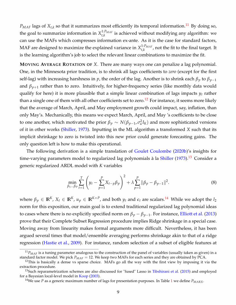
MOVING AVERAGE ROTATION OF X. There are many ways one can penalize a lag polynomial.
One, in the Minnesota prior tradition, is to shrink all lags coefficients to zero (except for the first
self-lag) with increasing harshness in p, the order of the lag. Another is to shrink each βp to βp−1
and βp+1 rather than to zero. Intuitively, for higher-frequency series (like monthly data would
qualify for here) it is more plausible that a simple linear combination of lags impacts yt rather
than a single one of them with all other coefficients set to zero.12 For instance, it seems more likely
that the average of March, April, and May employment growth could impact, say, inflation, than
only May’s. Mechanically, this means we expect March, April, and May ’s coefficients to be close
to one another, which motivated the prior βp ∼ N(βp−1, σ2u IK) and more sophisticated versions
of it in other works (Shiller, 1973). Inputting in the ML algorithm a transformed X such that its
implicit shrinkage to zero is twisted into this new prior could generate forecasting gains. The
only question left is how to make this operational.
The following derivation is a simple translation of Goulet Coulombe (2020b)’s insights for
time-varying parameters model to regularized lag polynomials à la Shiller (1973).13 Consider a
generic regularized ARDL model with K variables
minβ1...βP
T
∑t=1
(yt −
P
∑p=1
Xt−pβp
)2
+ λP
∑p=1‖βp − βp−1‖2. (8)
where βp ∈ IRK, Xt ∈ IRK, up ∈ IRK×P, and both yt and εt are scalars.14 While we adopt the l2norm for this exposition, our main goal is to extend traditional regularized lag polynomial ideas
to cases where there is no explicitly specified norm on βp − βp−1. For instance, Elliott et al. (2013)
prove that their Complete Subset Regression procedure implies Ridge shrinkage in a special case.
Moving away from linearity makes formal arguments more difficult. Nevertheless, it has been
argued several times that model/ensemble averaging performs shrinkage akin to that of a ridge
regression (Hastie et al., 2009). For instance, random selection of a subset of eligible features at
11PMAF is a tuning parameter analogous to the construction of the panel of variables (usually taken as given) in astandard factor model. We pick PMAF = 12. We keep two MAFs for each series and they are obtained by PCA.
12This is basically a dense vs sparse choice. MAFs go all the way with the first view by imposing it via theextraction procedure.
13Such reparametrization schemes are also discussed for "fused" Lasso in Tibshirani et al. (2015) and employedfor a Bayesian local-level model in Koop (2003).
14We use P as a generic maximum number of lags for presentation purposes. In Table 1 we define PMARX .
9
each split encourage each feature to be included in the predictive function, but in a moderate
fashion.15 The resulting "implicit" coefficient is an average of specifications that included the
regressor and some that did not. In the latter case, the coefficient is always zero by construction.
Hence, the ensemble shrinks contributions towards zero and the so-called mtry hyperparameter
guides the level of shrinkage like a bandwidth parameter would (Olson and Wyner, 2018).
To get implicit regularized lag polynomial shrinkage, we now rewrite problem (8) as a ridge
regression. For all derivations to come, it is less tedious to turn to matrix notations. The Fused
Ridge problem is now written as
minβ
(y− Xβ)′ (y− Xβ) + λβ′D′Dβ
where D is the first difference operator. The first step is to reparametrize the problem by using
the relationship βk = Cθk that we have for all k regressors. C is a lower triangular matrix of ones
(for the random walk case) and define θk = [uk β0,k]. For the simple case of one parameter and
P = 4: β0β1β2β3
=
1 0 0 01 1 0 01 1 1 01 1 1 1
β0u1u2u3
.
For the general case of K parameters, we have
β = Cθ, C ≡ IK ⊗ C
and θ is just stacking all the θk into one long vector of length KP. Using the reparametrization
β = Cθ, the Fused Ridge problem becomes
minθ
(y− XCθ)′ (y− XCθ) + λθ′C′D′DCθ.
Let Z ≡ XC and use the fact that D = C−1 to obtain the Ridge regression problem
minθ
(y− Zθ)′ (y− Zθ) + λθ′θ. (9)
We arrived at destination. Using Z rather than X in an algorithm that performs shrinkage will
implicitly shrink βp to βp−1 rather than to 0. This is obviously much more convenient than modi-
fying the algorithm itself and is directly applicable to any algorithm using time series data as input.
One question remains: what is Z, exactly? For a single polynomial at time t, we have Zt,k = Xt,kC.
15Recently, (Goulet Coulombe, 2020c) argued that ensemble averaging methods à la RF prunes a latent tree. Fol-lowing this view, the need for cleverly pre-assembled data combinations is even clearer.
10
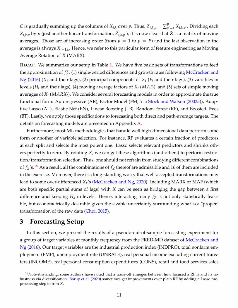
C is gradually summing up the columns of Xt,k over p. Thus, Zt,k,p = ∑Pp′=1 Xt,k,p′ . Dividing each
Zt,k,p by p (just another linear transformation, Zt,k,p ), it is now clear that Z is a matrix of moving
averages. Those are of increasing order (from p = 1 to p = P) and the last observation in the
average is always Xt−1,k. Hence, we refer to this particular form of feature engineering as Moving
Average Rotation of X (MARX).
RECAP. We summarize our setup in Table 1. We have five basic sets of transformations to feed
the approximation of f ∗Z: (1) single-period differences and growth rates following McCracken and
Ng (2016) (Xt and their lags), (2) principal components of Xt (Ft and their lags), (3) variables in
levels (Ht and their lags), (4) moving average factors of Xt (MAFt), and (5) sets of simple moving
averages of Xt (MARXt). We consider several forecasting models in order to approximate the true
functional form: Autoregressive (AR), Factor Model (FM, à la Stock and Watson (2002a)), Adap-
tive Lasso (AL), Elastic Net (EN), Linear Boosting (LB), Random Forest (RF), and Boosted Trees
(BT). Lastly, we apply those specifications to forecasting both direct and path-average targets. The
details on forecasting models are presented in Appendix A.
Furthermore, most ML methodologies that handle well high-dimensional data perform some
form or another of variable selection. For instance, RF evaluates a certain fraction of predictors
at each split and selects the most potent one. Lasso selects relevant predictors and shrinks oth-
ers perfectly to zero. By rotating X, we can get these algorithms (and others) to perform restric-
tion/transformation selection. Thus, one should not refrain from studying different combinations
of fZ’s.16 As a result, all the combinations of fZ thereof are admissible and 16 of them are included
in the exercise. Moreover, there is a long-standing worry that well-accepted transformations may
lead to some over-differenced Xk’s (McCracken and Ng, 2020). Including MARX or MAF (which
are both specific partial sums of lags) with X can be seen as bridging the gap between a first
difference and keeping Hk in levels. Hence, interacting many fZ is not only statistically feasi-
ble, but econometrically desirable given the sizable uncertainty surrounding what is a "proper"
transformation of the raw data (Choi, 2015).
3 Forecasting Setup
In this section, we present the results of a pseudo-out-of-sample forecasting experiment for
a group of target variables at monthly frequency from the FRED-MD dataset of McCracken and
Ng (2016). Our target variables are the industrial production index (INDPRO), total nonfarm em-
ployment (EMP), unemployment rate (UNRATE), real personal income excluding current trans-
fers (INCOME), real personal consumption expenditures (CONS), retail and food services sales
16Notwithstanding, some authors have noted that a trade-off emerges between how focused a RF is and its ro-bustness via diversification. Borup et al. (2020) sometimes get improvements over plain RF by adding a Lasso pre-processing step to trim X.
11
Table 1: Model Specification Summary
Cases Feature Matrix Zt
F Zt :=[{Li−1Ft}
p f1
]F-X Zt :=
[{Li−1Ft}
p f1 , {Li−1Xt}pm
1
]F-MARX Zt :=
[{Li−1Ft}
p f1 , {MARXi
yt}py1 , {MARXi
1t}pm1 , . . . , {MARXi
Kt}pm1
]F-MAF Zt :=
[{Li−1Ft}
p f1 , {MAFi
yt}rK1 , {MAFi
1t}rK1 , . . . , {MAFi
Kt}rK1
]F-Level Zt :=
[{Li−1Ft}
p f1 , Yt, Ht
]F-X-MARX Zt :=
[{Li−1Ft}
p f1 , {Li−1Xt}pm
1 , {MARXiyt}
py1 , {MARXi
1t}pm1 , . . . , {MARXi
Kt}pm1
]F-X-MAF Zt :=
[{Li−1Ft}
p f1 , {Li−1Xt}pm
1 , {MAFiyt}
rK1 , {MAFi
1t}rK1 , . . . , {MAFi
Kt}rK1
]F-X-Level Zt :=
[{Li−1Ft}
p f1 , {Li−1Xt}pm
1 , Yt, Ht
]F-X-MARX-Level Zt :=
[{Li−1Ft}
p f1 , {Li−1Xt}pm
1 , {MARXiyt}
py1 , {MARXi
1t}pm1 , . . . , {MARXi
Kt}pm1 , Yt, Ht
]X Zt :=
[{Li−1Xt}pm
1
]MARX Zt :=
[{MARXi
yt}py1 , {MARXi
1t}pm1 , . . . , {MARXi
Kt}pm1
]MAF Zt :=
[{MAFi
yt}rK1 , {MAFi
1t}rK1 , . . . , {MAFi
Kt}rK1
]X-MARX Zt :=
[{Li−1Xt}pm
1 , {MARXiyt}
py1 , {MARXi
1t}pm1 , . . . , {MARXi
Kt}pm1
]X-MAF Zt :=
[{Li−1Xt}pm
1 , {MAFiyt}
rK1 , {MAFi
1t}rK1 , . . . , {MAFi
Kt}rK1
]X-Level Zt :=
[{Li−1Xt}pm
1 , Yt, Ht
]X-MARX-Level Zt :=
[{Li−1Xt}pm
1 , {MARXiyt}
py1 , {MARXi
1t}pm1 , . . . , {MARXi
Kt}pm1 , Yt, Ht
]Note: This table show the combinations of data transformation used to assess the individual marginal contribution of each fZ . Lags ofmonth-to-month (log)-change of the series to forecast are always included.
(RETAIL), housing starts (HOUST), M2 money stock (M2), consumer price index (CPI), and the
production price index (PPI). Given that we make predictions at horizons of 1, 3, 6, 9, 12, and
24 months, we are effectively targeting the average growth rate over those periods, except for
the unemployment rate for which we target average differences. These series are representative
macroeconomic indicators of the US economy, as stated in Kim and Swanson (2018), which is also
based on Goulet Coulombe et al. (2019) exercise for many ML models, itself based on Kotchoni
et al. (2019) and a whole literature of extensive horse races in the spirit of Stock and Watson (1998).
The POOS period starts in January of 1980 and ends in December of 2017. We use an expanding
window for estimation starting from 1960M01. Following standard practice in the literature, we
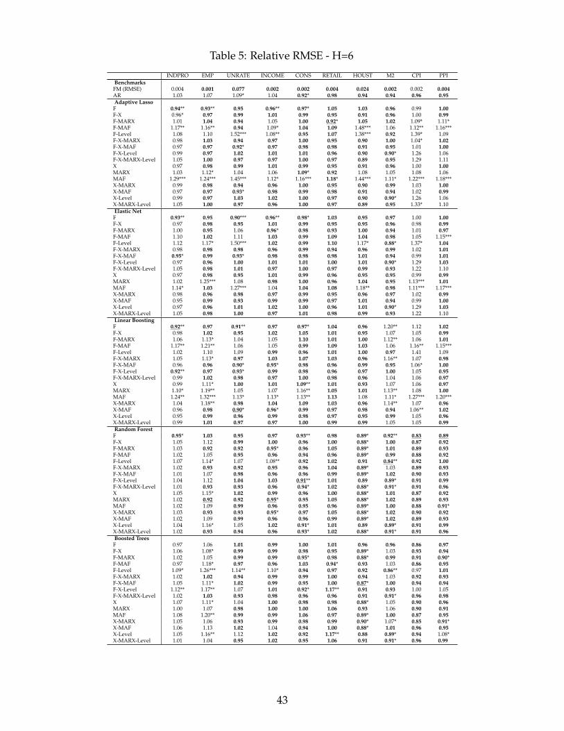
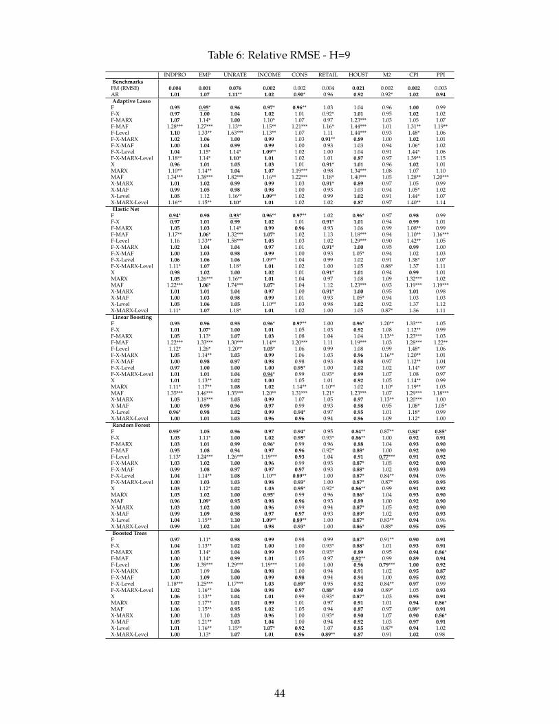
evaluate the quality of point forecasts using the root Mean Square Error (RMSE). For the fore-
casted value at time t of variable v made h steps before, we compute
RMSEv,h,m =
√1
#OOS ∑t∈OOS
(yvt − yv,h,m
t−h )2 (10)
The standard Diebold and Mariano (2002) (DM) test procedure is used to compare the predictive
accuracy of each model against the reference factor model (FM). RMSE is the most natural loss
12
function given that all models are trained to minimize the squared loss in-sample. We also imple-
ment the Model Confidence Set (MCS) that selects the subset of best models at a given confidence
level (Hansen et al., 2011).
Hyperparameter selection is performed using the BIC for AR and FM and K-fold cross-validation
is used for the remaining models. This approach is theoretically justified in time series models
under conditions spelled out by Bergmeir et al. (2018). Moreover, Goulet Coulombe et al. (2019)
compared it with a scheme which respects the time structure of the data and found K-fold to
be performing as well as or better than this alternative scheme. All models are estimated every
month while their hyperparameters are reoptimized every two years.
4 Results
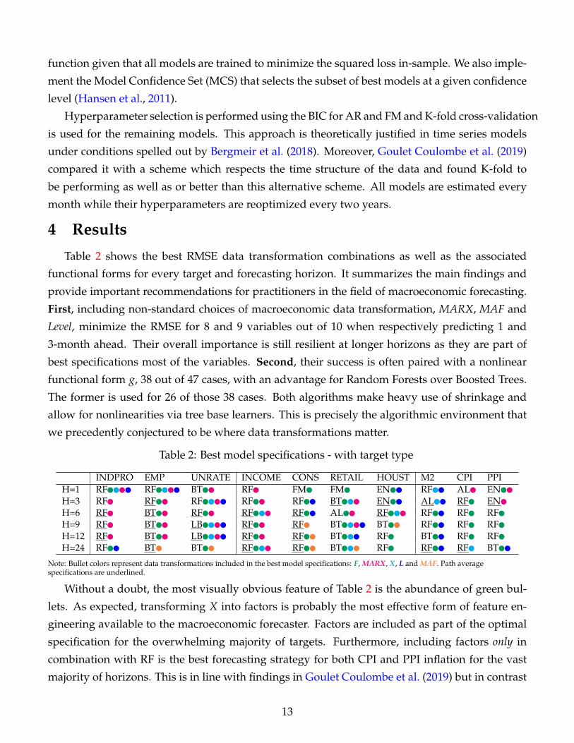
Table 2 shows the best RMSE data transformation combinations as well as the associated
functional forms for every target and forecasting horizon. It summarizes the main findings and
provide important recommendations for practitioners in the field of macroeconomic forecasting.
First, including non-standard choices of macroeconomic data transformation, MARX, MAF and
Level, minimize the RMSE for 8 and 9 variables out of 10 when respectively predicting 1 and
3-month ahead. Their overall importance is still resilient at longer horizons as they are part of
best specifications most of the variables. Second, their success is often paired with a nonlinear
functional form g, 38 out of 47 cases, with an advantage for Random Forests over Boosted Trees.
The former is used for 26 of those 38 cases. Both algorithms make heavy use of shrinkage and
allow for nonlinearities via tree base learners. This is precisely the algorithmic environment that
we precedently conjectured to be where data transformations matter.
Table 2: Best model specifications - with target type
Note: Bullet colors represent data transformations included in the best model specifications: F, MARX, X, L and MAF. Path averagespecifications are underlined.
Without a doubt, the most visually obvious feature of Table 2 is the abundance of green bul-
lets. As expected, transforming X into factors is probably the most effective form of feature en-
gineering available to the macroeconomic forecaster. Factors are included as part of the optimal
specification for the overwhelming majority of targets. Furthermore, including factors only in
combination with RF is the best forecasting strategy for both CPI and PPI inflation for the vast
majority of horizons. This is in line with findings in Goulet Coulombe et al. (2019) but in contrast
13
with the results found in Medeiros et al. (2019). The major difference with the latter is that they
estimate and evaluate models on the basis of single month inflation rate, which is only the inter-
mediary step in our path average strategy. In addition, we explore the possibility that F alone
could be better than X, rather than always both together. As it turns out, the winning combina-
tion is RF using factors as sole inputs to directly target the average growth. Finally, the omission
of factors from optimal specifications for industrial production growth 3 to 12 months ahead is
naturally surprising. This points out that current wisdom based on linear models may not be
directly applicable to nonlinear ones. In fact, alternative rotations will sometimes do better.
There is plentiful of red bullets populating the top rows of Table 2. Indeed, our most salient
new transformation is MARX. In combination with nonlinear tree-based models, it contributes to
improve forecasting accuracy for real activity series such as industrial production, employment,
unemployment rate, and income, while they are best paired with penalized regressions to predict
the CPI and PPI inflation rates. The dominance of MARX is particularly striking for real activity
series as the transformation is included in every best specification for those variables at all horizons
ranging from one month to a year. We further investigate how those RMSE gains materialize in
terms of forecasts around key periods in section 4.2. While MAF performance is often positively
correlated with MARX, the latter is usually the better of the two, except for longer-run forecasts –
like those 2-years where MAF is featured for four variables.
Considering levels is particularly important for the M2 money stock as it is included in the
best model for all horizons. For other variables, its pertinence is rather sporadic, with at least two
horizons featuring it for INDPRO, UNRATE, CONS, and RETAIL.
The preference for ydirectt+h vs ypath-avg
t+h mostly go on a variable by variable basis. However, there
is clear consensus ypath-avgt+h � ydirect
t+h for all variables which strongly co-move with the business
cycle (INDPRO, EMP, UNRATE, INCOME, CONS) with the notable exception of retail sales and
housing starts. When it comes to nominal targets (M2, CPI, PPI), ypath-avgt+h ≺ ydirect
t+h is unanimous
for horizons 6 to 12 months, and so are the affiliated data transformations as well as the g choice
(all tree ensembles, with 8 out of 9 being RF). The quantitative importance of both types of gains
on both sides is studied in section 4.1, while section 4.2 looks at implied forecasts to understand
when and why ypath-avgt+h � ydirect
t+h , or the reverse.
These findings are particularly important given the increasing interest in ML macro forecast-
ing. They suggest that traditional data transformations, meant to achieve stationarity, do leave
substantial forecasting gains on the practitioners’ table. These losses can be successfully recov-
ered by combining ML methods with well-motivated rotations of predictors such as MARX and
MAF (or sometimes by simply including variables in levels) and by constructing the final forecast
by the path average approach.
The previous results were desirably expeditive. The detailed results on the underlying perfor-
14
mance gains and their statistical significance are presented in Appendix B.
4.1 Marginal Contribution of Data Pre-processing
In order to disentangle marginal effects of data transformations on forecast accuracy we run
the following regression inspired by Carriero et al. (2019) and Goulet Coulombe et al. (2019):
R2t,h,v,m = αF + ψt,v,h + vt,h,v,m, (11)
where R2t,h,v,m ≡ 1 − e2
t,h,v,m1T ∑T
t=1(yv,t+h−yv,h)2 is the pseudo-out-of-sample R2, and e2t,h,v,m are squared
prediction errors of model m for variable v and horizon h at time t. ψt,v,h is a fixed effect term that
demeans the dependent variable by “forecasting target,” that is a combination of t, v, and h. αF
is a vector of αMARX, αMAF, and αF terms associated to each new data transformation considered
in this paper, as well as to the factor model. H0 is α f = 0 ∀ f ∈ F = [MARX, MAF, F]. In
other words, the null is that there is no predictive accuracy gain with respect to a base model that
does not have this particular data pre-processing. While the generality of (11) is appealing, when
investigating the heterogeneity of specific partial effects, it will be much more convenient to run
specific regressions for the multiple hypothesis we wish to test. That is, to evaluate a feature f ,
we run
∀m ∈ M f : R2t,h,v,m = α f + ψt,v,h + vt,h,v,m (12)
whereM f is defined as the set of models that differs only by the feature under study f .
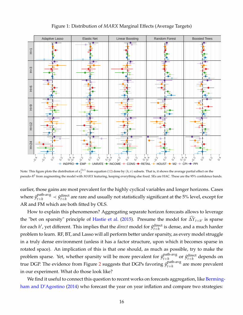
MARX. Figure 1 plots the distribution of α(h,v)MARX from equation (11) done by (h, v) subsets. Hence,
we allow for heterogeneous effects of the MARX transformation according to 60 different targets.
The marginal contribution of MARX on the pseudo-R2 depends a lot on models, horizons, and
series. However, we remark that at the short-run horizons, when combined with nonlinear meth-
ods, it produces positive and significant effects. It particularly improves the forecast accuracy
for real activity series like industrial production, labor market series and income, even at larger
horizons. For instance, the gains from using MARX with RF achieve 16% when predicting IND-
PRO at the h = 3 horizon, and 14% in the case of employment if h = 6. When used with linear
methods, the estimates are more often on the negative side, except for inflation rates and M2 at
short horizons, and a few special cases at the one and two-year ahead horizons.
DIRECT VS PATH AVERAGE. Figure 2 reports the most unequivocal result of this paper: ydirectt+h can
prove largely suboptimal to ypath-avgt+h . For every method using a high-dimensional Zt shrunk in
some way, i.e., not the OLS-based AR and FM, ypath-avgt+h will do significantly better than the direct
approach, with α(h,v)path-avg sometimes around 30% and highly statistically significant. As mentioned
15
Figure 1: Distribution of MARX Marginal Effects (Average Targets)
●
●
●
●
●
●
●
●●
●
●
●
●
●
●
●
●
●●
●
●
●
●
●
●
●
●
●●
●
●
●
●
●
●
●
●
●●
●
●
●
●
●
●
●
●
●●
●
●
●
●
●
●
●
●
●●
●
●
●
●
●
●
●
●
●●
●
●
●
●
●
●
●
●
●●
●
●
●
●
●
●
●
●
●●
●
●
●
●
●
●
●
●
●●
●
●
●
●
●
●
●
●
●●
●
●
●
●
●
●
●
●
●●
●
●
●
●
●
●
●
●
●●
●
●
●
●
●
●
●
●
●●
●
●
●
●
●
●
●
●
●●
●
●
●
●
●
●
●
●
●●
●
●
●
●
●
●
●
●
●●
●
●
●
●
●
●
●
●
●●
●
●
●
●
●
●
●
●
●●
●
●
●
●
●
●
●
●
●●
●
●
●
●
●
●
●
●
●●
●
●
●
●
●
●
●
●
●●
●
●
●
●
●
●
●
●
●●
●
●
●
●
●
●
●
●
●●
●
●
●
●
●
●
●
●
●●
●
●
●
●
●
●
●
●
●●
●
●
●
●
●
●
●
●
●●
●
●
●
●
●
●
●
●
●●
●
●
●
●
●
●
●
●
●●
●
●
●
●
●
●
●
●
●●
●
Adaptive Lasso Elastic Net Linear Boosting Random Forest Boosted Trees
H=
1H
=3
H=
6H
=9
H=
12
H=
24
−0.4
−0.2 0.0
0.2
0.4
−0.4
−0.2 0.0
0.2
0.4
−0.4
−0.2 0.0
0.2
0.4
−0.4
−0.2 0.0
0.2
0.4
−0.4
−0.2 0.0
0.2
0.4
● ● ● ● ● ● ● ● ● ●INDPRO EMP UNRATE INCOME CONS RETAIL HOUST M2 CPI PPI
Note: This figure plots the distribution of α(h,v)f from equation (12) done by (h, v) subsets. That is, it shows the average partial effect on the
pseudo-R2 from augmenting the model with MARX featuring, keeping everything else fixed. SEs are HAC. These are the 95% confidence bands.
earlier, those gains are most prevalent for the highly cyclical variables and longer horizons. Cases
where ypath-avgt+h ≺ ydirect
t+h are rare and usually not statistically significant at the 5% level, except for
AR and FM which are both fitted by OLS.
How to explain this phenomenon? Aggregating separate horizon forecasts allows to leverage
the "bet on sparsity" principle of Hastie et al. (2015). Presume the model for ∆Yt+h′ is sparse
for each h′, yet different. This implies that the direct model for ydirectt+h is dense, and a much harder
problem to learn. RF, BT, and Lasso will all perform better under sparsity, as every model struggle
in a truly dense environment (unless it has a factor structure, upon which it becomes sparse in
rotated space). An implication of this is that one should, as much as possible, try to make the
problem sparse. Yet, whether sparsity will be more prevalent for ypath-avgt+h or ydirect
t+h depends on
true DGP. The evidence from Figure 2 suggests that DGPs favoring ypath-avgt+h are more prevalent
in our experiment. What do those look like?
We find it useful to connect this question to recent works on forecasts aggregation, like Berming-
ham and D’Agostino (2014) who forecast the year on year inflation and compare two strategies:
16
Figure 2: Distribution of Marginal Effects of Target Transformation
●
●
●
●
●
●
●
●●
●
●
●
●
●
●
●
●
●●
●
●
●
●
●
●
●
●
●●
●
●
●
●
●
●
●
●
●●
●
●
●
●
●
●
●
●
●●
●
●
●
●
●
●
●
●
●●
●
●
●
●
●
●
●
●
●●
●
●
●
●
●
●
●
●
●●
●
●
●
●
●
●
●
●
●●
●
●
●
●
●
●
●
●
●●
●
●
●
●
●
●
●
●
●●
●
●
●
●
●
●
●
●
●●
●
●
●
●
●
●
●
●
●●
●
●
●
●
●
●
●
●
●●
●
●
●
●
●
●
●
●
●●
●
●
●
●
●
●
●
●
●●
●
●
●
●
●
●
●
●
●●
●
●
●
●
●
●
●
●
●●
●
●
●
●
●
●
●
●
●●
●
●
●
●
●
●
●
●
●●
●
●
●
●
●
●
●
●
●●
●
●
●
●
●
●
●
●
●●
●
●
●
●
●
●
●
●
●●
●
●
●
●
●
●
●
●
●●
●
●
●
●
●
●
●
●
●●
●
●
●
●
●
●
●
●
●●
●
●
●
●
●
●
●
●
●●
●
●
●
●
●
●
●
●
●●
●
●
●
●
●
●
●
●
●●
●
●
●
●
●
●
●
●
●●
●
●
●
●
●
●
●
●
●●
●
●
●
●
●
●
●
●
●●
●
●
●
●
●
●
●
●
●●
●
●
●
●
●
●
●
●
●●
●
●
●
●
●
●
●
●
●●
●
AR FM Adaptive Lasso Elastic Net Linear Boosting Random Forest Boosted Trees
H=
3H
=6
H=
9H
=1
2H
=2
4−0
.6−0
.3 0.0
0.3
0.6
−0.6
−0.3 0.0
0.3
0.6
−0.6
−0.3 0.0
0.3
0.6
−0.6
−0.3 0.0
0.3
0.6
−0.6
−0.3 0.0
0.3
0.6
−0.6
−0.3 0.0
0.3
0.6
−0.6
−0.3 0.0
0.3
0.6
● ● ● ● ● ● ● ● ● ●INDPRO EMP UNRATE INCOME CONS RETAIL HOUST M2 CPI PPI
Note: This figure plots the distribution of α(h,v)f from equation (12) done by (h, v) subsets. That is, it shows the average partial effect on the
pseudo-R2 from accumulating single period predictions (ypath-avgt+h ) instead of targeting the average growth rate directly (ydirect
t+h ), keepingeverything else fixed. SEs are HAC. These are the 95% confidence bands.
forecasting overall inflation directly vs forecasting individual elements of the consumption basket
and using a weighted average of forecasts. They find that using more components and aggregat-
ing individual forecasts improves performance.17 They provide a simple example to rationalize
their result: forecasting an aggregate variable made of two series with differing levels of persis-
tence using only past values of the aggregate will be misspecified. In ML forecasting context,
where Z contains "everything" anyway, this problem translates from misspecification into mak-
ing once sparse problems into a dense one, which is harder to learn. Consider a toy multi-horizon
problem∆Yt+h′ = βhXt,k∗(h′) + εt+h′ , h′ = 1, 2
yt+2 =∆Yt+2 + ∆Yt+1
2
⇒ yt+2 =β1
2Xt,k∗(1) +
β2
2Xt,k∗(2) +
εt+1 + εt+2
2.
(13)
17In a similar vein, Marcellino et al. (2003) found that forecasting inflation at the country level and then aggregat-ing the forecasts increases does better than forecasting at the aggregate level (Euro).
17
where one needs to select a single predictor for each horizon. In this simple analogy to a high-
dimensional problem, unless k∗(1) = k∗(2), that is, the optimally selected regressor is the same
for both horizon, the direct approach implies a "denser" problem – estimating two coefficients
rather than one for separate regressions. A scaled-up version of this is that if each horizon along
the path implies 25 non-overlapping predictors, then the average growth rate model should have
25× h predictors, a much harder learning problem.
Of course, the ydirectt+h approach might work better, even in a ML environment. For instance,
the "aggregated" error term in (13) could have a lower variance if Corr(εt+1, εt+2) < 0. Note
that this would not imply substantial differences in the OLS paradigm since such errors would
rather average out at the aggregation step in ypath-avgt+h . However, if a regularization level must
be picked by cross-validation (like Lasso’s λ), an environment where there is a strong common
component across h′’s for the conditional mean could favor ydirectt+h . The reason for this is that
choosing a regularization level optimized for a single horizon h′ could be different than what
may be optimal for the final averaged prediction – as examplified by our ridge regression case
of equations (4) and (5). This observation is closely related to that of Granger (1987) who shows
that the behavior of the aggregate series can easily be dominated by a common component even
if it is unimportant for each of the microeconomic unit being aggregated. Translated to our ML-
based multi-horizon problem, this means we want to avoid having overly harsh regularization
throwing out negligible effects for a given h′ whose accumulation over all h′’s makes them in
fact non-negligible. Thus, if the noise level is much higher for single horizons forecasts, an overly
strong λh′ for each h′may be chosen whereas λh for ydirectt+h could be milder and allow for otherwise
neglected signals to come through.
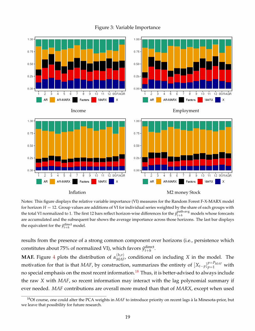
These potential explanations are illustrated using variable importance (VI) in Figure 3. As
shown earlier, the path average approach has outperformed the direct one when predicting real
activity variables. VI measures in top panels show how models for ypath-avgt+h use a much more
polarized set of variables whereas those aiming for ydirectt+h using a very diverse set of predictors
in case of Income and Employment. This shed light on our bet-on-sparsity conjecture, i.e. that
ypath-avgt+h will have the upper hand if ∆Yt+h′ predictive problems are quite heterogenous. In both
cases, horizon 1 is quite different from 2-3-4, which also differ from the 5-12 block. It is noted in
Figures 8 and 15 that ypath-avgt+h visibly demonstrate a better capacity for autoregressive behavior
(even at h = 12) which provides it with a clear edge over ydirectt+h during recessions. Interestingly,
the foundation for this finding is also visible in Figure 3 for real activity variables: ypath-avgt+h reliance
on plain AR terms is more than twice that of ydirectt+h .
The bottom panels show VI measures for CPI inflation and M2 growth. Recall that ypath-avgt+h ≺
ydirectt+h was unambiguous for those variables. Here again, results are in line with the above ar-
guments. The retained predictors’ sets are much more similar across the two approaches, which
18
Figure 3: Variable Importance
Income Employment
Inflation M2 money Stock
Notes: This figure displays the relative variable importance (VI) measures for the Random Forest F-X-MARX modelfor horizon H = 12. Group values are additions of VI for individual series weighted by the share of each groups withthe total VI normalized to 1. The first 12 bars reflect horizon-wise differences for the ypath-avg
t+h models whose forecastsare accumulated and the subsequent bar shows the average importance across those horizons. The last bar displaysthe equivalent for the ydirect
t+h model.
results from the presence of a strong common component over horizons (i.e., persistence which
constitutes about 75% of normalized VI), which favors ydirectt+h .
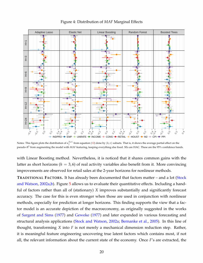
MAF. Figure 4 plots the distribution of α(h,v)MAF, conditional on including X in the model. The
motivation for that is that MAF, by construction, summarizes the entirety of [Xt−p]p=PMAFp=1 with
no special emphasis on the most recent information.18 Thus, it is better-advised to always include
the raw X with MAF, so recent information may interact with the lag polynomial summary if
ever needed. MAF contributions are overall more muted than that of MARX, except when used
18Of course, one could alter the PCA weights in MAF to introduce priority on recent lags à la Minesota-prior, butwe leave that possibility for future research.
19
Figure 4: Distribution of MAF Marginal Effects
●
●
●
●
●
●
●
●●
●
●
●
●
●
●
●
●
●●
●
●
●
●
●
●
●
●
●●
●
●
●
●
●
●
●
●
●●
●
●
●
●
●
●
●
●
●●
●
●
●
●
●
●
●
●
●●
●
●
●
●
●
●
●
●
●●
●
●
●
●
●
●
●
●
●●
●
●
●
●
●
●
●
●
●●
●
●
●
●
●
●
●
●
●●
●
●
●
●
●
●
●
●
●●
●
●
●
●
●
●
●
●
●●
●
●
●
●
●
●
●
●
●●
●
●
●
●
●
●
●
●
●●
●
●
●
●
●
●
●
●
●●
●
●
●
●
●
●
●
●
●●
●
●
●
●
●
●
●
●
●●
●
●
●
●
●
●
●
●
●●
●
●
●
●
●
●
●
●
●●
●
●
●
●
●
●
●
●
●●
●
●
●
●
●
●
●
●
●●
●
●
●
●
●
●
●
●
●●
●
●
●
●
●
●
●
●
●●
●
●
●
●
●
●
●
●
●●
●
●
●
●
●
●
●
●
●●
●
●
●
●
●
●
●
●
●●
●
●
●
●
●
●
●
●
●●
●
●
●
●
●
●
●
●
●●
●
●
●
●
●
●
●
●
●●
●
●
●
●
●
●
●
●
●●
●
Adaptive Lasso Elastic Net Linear Boosting Random Forest Boosted Trees
H=
1H
=3
H=
6H
=9
H=
12
H=
24
−0.4
−0.2 0.0
0.2
0.4
−0.4
−0.2 0.0
0.2
0.4
−0.4
−0.2 0.0
0.2
0.4
−0.4
−0.2 0.0
0.2
0.4
−0.4
−0.2 0.0
0.2
0.4
● ● ● ● ● ● ● ● ● ●INDPRO EMP UNRATE INCOME CONS RETAIL HOUST M2 CPI PPI
Notes: This figure plots the distribution of α(h,v)f from equation (12) done by (h, v) subsets. That is, it shows the average partial effect on the
pseudo-R2 from augmenting the model with MAF featuring, keeping everything else fixed. SEs are HAC. These are the 95% confidence bands.
with Linear Boosting method. Nevertheless, it is noticed that it shares common gains with the
latter as short horizons (h = 3, 6) of real activity variables also benefit from it. More convincing
improvements are observed for retail sales at the 2-year horizons for nonlinear methods.
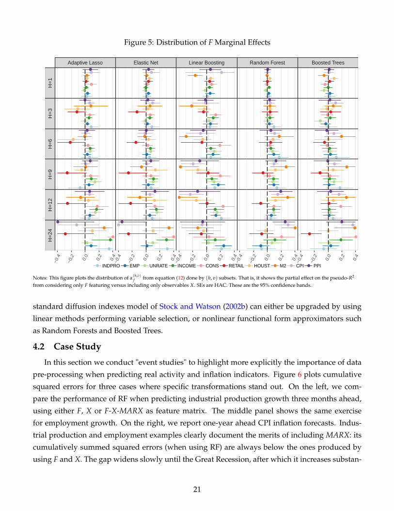
TRADITIONAL FACTORS. It has already been documented that factors matter – and a lot (Stock
and Watson, 2002a,b). Figure 5 allows us to evaluate their quantitative effects. Including a hand-
ful of factors rather than all of (stationary) X improves substantially and significantly forecast
accuracy. The case for this is even stronger when those are used in conjunction with nonlinear
methods, especially for prediction at longer horizons. This finding supports the view that a fac-
tor model is an accurate depiction of the macroeconomy, as originally suggested in the works
of Sargent and Sims (1977) and Geweke (1977) and later expanded in various forecasting and
structural analysis applications (Stock and Watson, 2002a; Bernanke et al., 2005). In this line of
thought, transforming X into F is not merely a mechanical dimension reduction step. Rather,
it is meaningful feature engineering uncovering true latent factors which contains most, if not
all, the relevant information about the current state of the economy. Once F’s are extracted, the
20
Figure 5: Distribution of F Marginal Effects
●
●
●
●
●
●
●
●●
●
●
●
●
●
●
●
●
●●
●
●
●
●
●
●
●
●
●●
●
●
●
●
●
●
●
●
●●
●
●
●
●
●
●
●
●
●●
●
●
●
●
●
●
●
●
●●
●
●
●
●
●
●
●
●
●●
●
●
●
●
●
●
●
●
●●
●
●
●
●
●
●
●
●
●●
●
●
●
●
●
●
●
●
●●
●
●
●
●
●
●
●
●
●●
●
●
●
●
●
●
●
●
●●
●
●
●
●
●
●
●
●
●●
●
●
●
●
●
●
●
●
●●
●
●
●
●
●
●
●
●
●●
●
●
●
●
●
●
●
●
●●
●
●
●
●
●
●
●
●
●●
●
●
●
●
●
●
●
●
●●
●
●
●
●
●
●
●
●
●●
●
●
●
●
●
●
●
●
●●
●
●
●
●
●
●
●
●
●●
●
●
●
●
●
●
●
●
●●
●
●
●
●
●
●
●
●
●●
●
●
●
●
●
●
●
●
●●
●
●
●
●
●
●
●
●
●●
●
●
●
●
●
●
●
●
●●
●
●
●
●
●
●
●
●
●●
●
●
●
●
●
●
●
●
●●
●
●
●
●
●
●
●
●
●●
●
●
●
●
●
●
●
●
●●
●
Adaptive Lasso Elastic Net Linear Boosting Random Forest Boosted Trees
H=
1H
=3
H=
6H
=9
H=
12
H=
24
−0.4
−0.2 0.0
0.2
0.4
−0.4
−0.2 0.0
0.2
0.4
−0.4
−0.2 0.0
0.2
0.4
−0.4
−0.2 0.0
0.2
0.4
−0.4
−0.2 0.0
0.2
0.4
● ● ● ● ● ● ● ● ● ●INDPRO EMP UNRATE INCOME CONS RETAIL HOUST M2 CPI PPI
Notes: This figure plots the distribution of α(h,v)f from equation (12) done by (h, v) subsets. That is, it shows the partial effect on the pseudo-R2
from considering only F featuring versus including only observables X. SEs are HAC. These are the 95% confidence bands.
standard diffusion indexes model of Stock and Watson (2002b) can either be upgraded by using
linear methods performing variable selection, or nonlinear functional form approximators such
as Random Forests and Boosted Trees.
4.2 Case Study
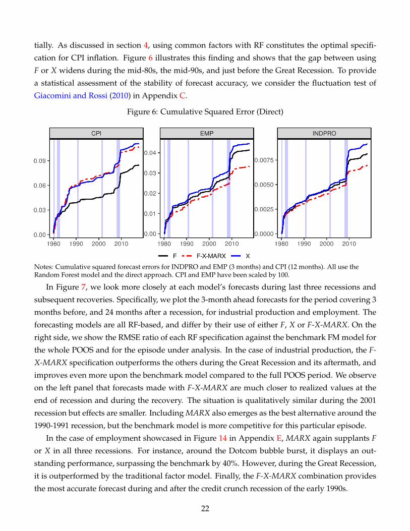
In this section we conduct "event studies" to highlight more explicitly the importance of data
pre-processing when predicting real activity and inflation indicators. Figure 6 plots cumulative
squared errors for three cases where specific transformations stand out. On the left, we com-
pare the performance of RF when predicting industrial production growth three months ahead,
using either F, X or F-X-MARX as feature matrix. The middle panel shows the same exercise
for employment growth. On the right, we report one-year ahead CPI inflation forecasts. Indus-
trial production and employment examples clearly document the merits of including MARX: its
cumulatively summed squared errors (when using RF) are always below the ones produced by
using F and X. The gap widens slowly until the Great Recession, after which it increases substan-
21
tially. As discussed in section 4, using common factors with RF constitutes the optimal specifi-
cation for CPI inflation. Figure 6 illustrates this finding and shows that the gap between using
F or X widens during the mid-80s, the mid-90s, and just before the Great Recession. To provide
a statistical assessment of the stability of forecast accuracy, we consider the fluctuation test of
Giacomini and Rossi (2010) in Appendix C.
Figure 6: Cumulative Squared Error (Direct)
Notes: Cumulative squared forecast errors for INDPRO and EMP (3 months) and CPI (12 months). All use theRandom Forest model and the direct approach. CPI and EMP have been scaled by 100.
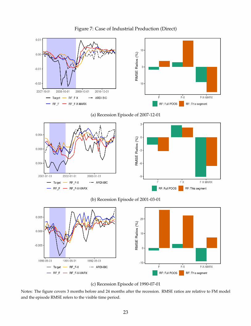
In Figure 7, we look more closely at each model’s forecasts during last three recessions and
subsequent recoveries. Specifically, we plot the 3-month ahead forecasts for the period covering 3
months before, and 24 months after a recession, for industrial production and employment. The
forecasting models are all RF-based, and differ by their use of either F, X or F-X-MARX. On the
right side, we show the RMSE ratio of each RF specification against the benchmark FM model for
the whole POOS and for the episode under analysis. In the case of industrial production, the F-
X-MARX specification outperforms the others during the Great Recession and its aftermath, and
improves even more upon the benchmark model compared to the full POOS period. We observe
on the left panel that forecasts made with F-X-MARX are much closer to realized values at the
end of recession and during the recovery. The situation is qualitatively similar during the 2001
recession but effects are smaller. Including MARX also emerges as the best alternative around the
1990-1991 recession, but the benchmark model is more competitive for this particular episode.
In the case of employment showcased in Figure 14 in Appendix E, MARX again supplants F
or X in all three recessions. For instance, around the Dotcom bubble burst, it displays an out-
standing performance, surpassing the benchmark by 40%. However, during the Great Recession,
it is outperformed by the traditional factor model. Finally, the F-X-MARX combination provides
the most accurate forecast during and after the credit crunch recession of the early 1990s.
22
Figure 7: Case of Industrial Production (Direct)
(a) Recession Episode of 2007-12-01
(b) Recession Episode of 2001-03-01
(c) Recession Episode of 1990-07-01
Notes: The figure covers 3 months before and 24 months after the recession. RMSE ratios are relative to FM modeland the episode RMSE refers to the visible time period.
23
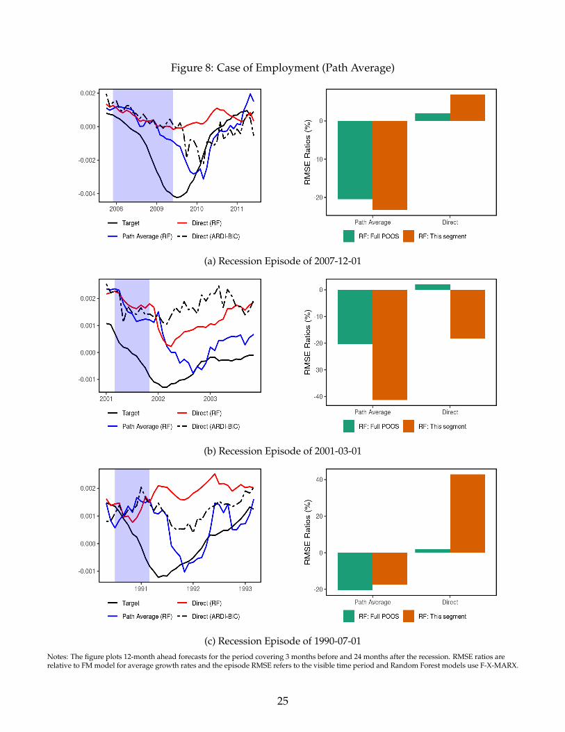
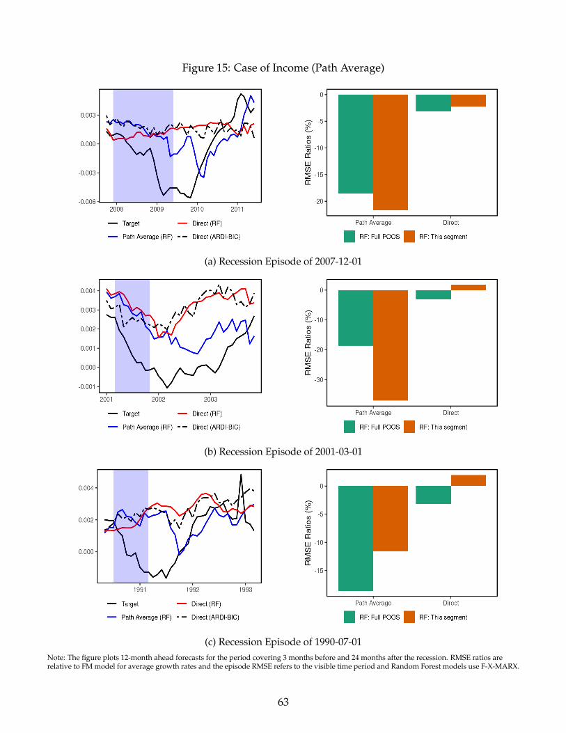
Figure 8 illustrate the relative performance of the two target transformations for employment
and income 12 months ahead. Again, we focus on the three most recent recession episodes.
ypath-avgt+h dramatically improves performance over ydirect
t+h and much of that edge visibly comes
from adjusting itself more or less rapidly to new economic conditions. In contrast, ydirectt+h is ex-
tremely smooth and report something close to the long-run average. Since the last three reces-
sions were characterized by a slow recovery, ypath-avgt+h procures much more credible forecasts of
employment and income simply by catching up sooner with realized values. This behavior is un-
derstandable through the lenses of Figure 3 where early horizons of ypath-avgt+h make a pronounced
use of autoregressive terms for both employment (and income, see Figure 15 in Appendix E).
4.3 Extraneous Transformations
We evaluate four additional data transformation strategies in combination with direct and
path average targets. First, we accommodate for the presence of error correction terms (ECM) by
considering the Factor-augmented ECM approach of Banerjee et al. (2014) and include level fac-
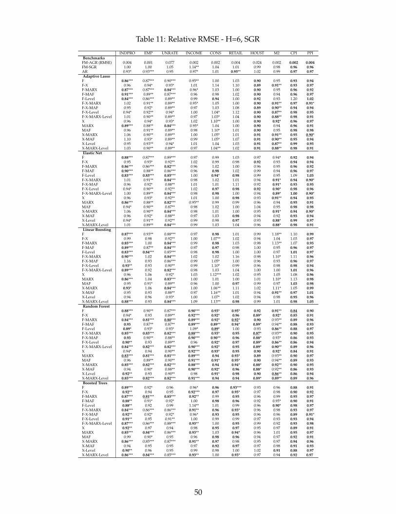
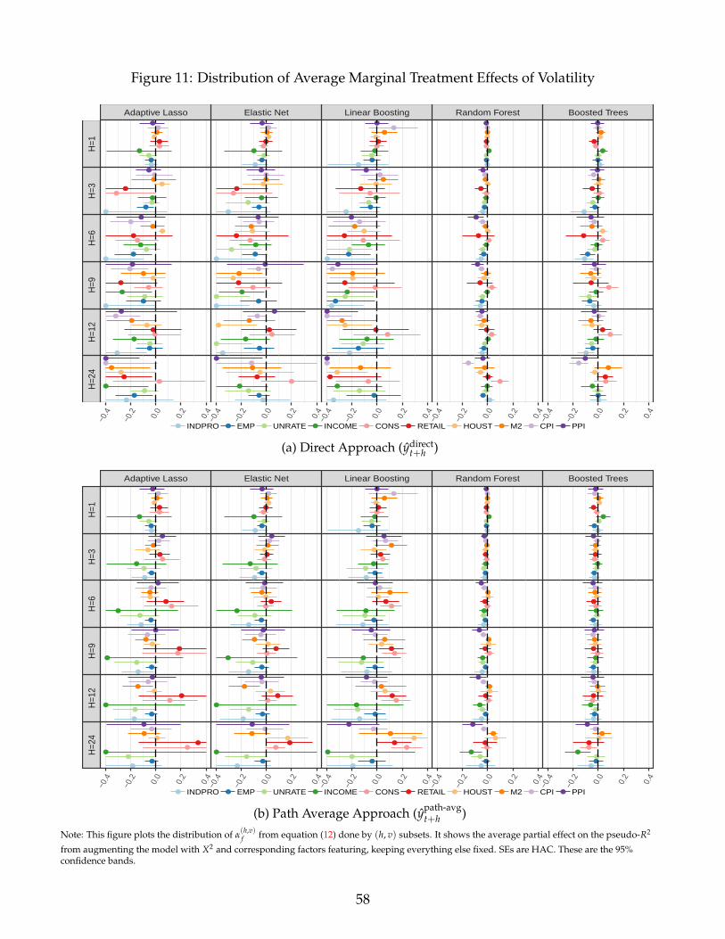
tors estimated from I(1) predictors. Second, we consider volatility factors and data inspired by
Gorodnichenko and Ng (2017), where both factors from X2 and X2 itself are included as predic-
tors. Third, we evaluate the potential predictive gains from including Forni et al. (2005)’s dynamic
factors in Z.
Figure 10, in Appendix D, reports the distribution of average marginal effects of adding level
factors in the predictors’ set Z. Their impact is generally small and not significant at short hori-
zons, while it depends on methods and forecasting approach at longer horizons. In the case of
the direct average approach, as depicted in panel 10a, adding level factors generally deteriorates
the predictive performance except for M2 with nonlinear methods. The effects are qualitatively
similar when the target is achieved by the path average approach, as shown in 10b.
Adding volatility data and factors is generally harmful with linear methods and has almost no
significant impact when random forest and boosted trees are used, see Figure 11.19 Hence, letting
ML methods generate nonlinearities proves to be more resilient than to include simple power
terms. This also suggests that volatility or other uncertainty proxies may not be the major sources
of nonlinearities for macroeconomic dynamics since they would otherwise be an indispensable
form of feature engineering which variable selection algorithms build their predictions from.
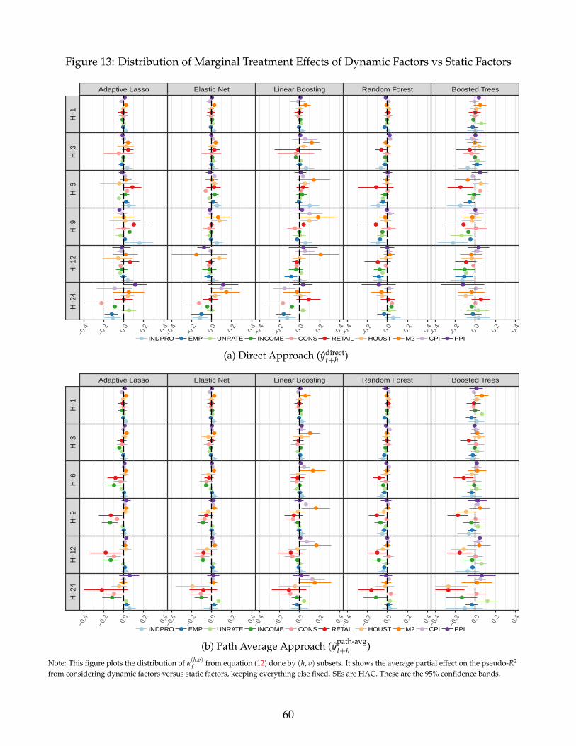
Finally, Figures 12 and 13 evaluate the marginal predictive content of dynamic factors as op-
posed to MAF and static factors (PCs) respectively. Considering dynamic factors as opposed to
MAF improves the predictability at longer horizons when used to construct ydirectt+h , while their
effects are rather small with ypath-avgt+h . When it comes to the choice between dynamic and static
19The very weak contribution of volatility terms to BT or RF is expected given that those transformations arelocally monotone (i.e, for all points where Xk,t > 0 or Xk,t < 0) and trees are invariant to monotone transformations.
24
Figure 8: Case of Employment (Path Average)
(a) Recession Episode of 2007-12-01
(b) Recession Episode of 2001-03-01
(c) Recession Episode of 1990-07-01Notes: The figure plots 12-month ahead forecasts for the period covering 3 months before and 24 months after the recession. RMSE ratios arerelative to FM model for average growth rates and the episode RMSE refers to the visible time period and Random Forest models use F-X-MARX.
25
factors, the results are in general quantitatively small but suggest that standard principal compo-
nents are preferred, especially in combination with nonlinear methods, which is analogous to the
findings of Boivin and Ng (2005) in linear environments.
5 Conclusion
This paper studies the virtues of standard and newly proposed data transformations for macroe-
conomic forecasting with machine learning. The classic transformations comprise the dimension
reduction of stationarized data by means of principal components and the inclusion of level vari-
ables in order to take into account low frequency movements. Newly proposed avenues include
moving average factors (MAF) and moving average rotation of X (MARX). The last two were mo-
tivated by the need to compress the information within a lag polynomial, especially if one desires
to keep X close to its original – interpretable – space. In addition to the aforementioned trans-
formations focusing on X, we considered two pre-processing alternatives for the target variable,
namely the direct and path average approaches.
To evaluate the contribution of data transformations for macroeconomic prediction, we have
considered three linear and two nonlinear ML methods (Elastic Net, Adaptive Lasso, Linear
Boosting, Random Forests and Boosted Trees) in a substantive pseudo-out-of-sample forecasting
exercise was done over 38 years for 10 key macroeconomic indicators and 6 horizons. With the
different permutations of fZ’s available from the above, we have analyzed a total of 15 different
information sets. The combination of standard and non-standard data transformations (MARX,
MAF, Level) is shown to minimize the RMSE, particularly at shorter horizons. Those consistent
gains are usually obtained when a nonlinear nonparametric ML algorithm is being used. This
is precisely the algorithmic environment we conjectured could benefit most from our proposed
fZ’s. Additionally, traditional factors are featured in the overwhelming majority of best informa-
tion sets for each target. Therefore, while ML methods can handle the high-dimensional X (both
computationally and statistically), extracting common factors remains straightforward feature
engineering that works.
The way the prediction is constructed can make a great difference. The path average approach
is more accurate than the direct one for almost all real activity variables (and at various horizons).
The gains can be as large as 30% and are mostly observed when the path average approach is
used in conjunction with regularization and/or nonparametric nonlinearity.
As the number of researchers and practitioners in the field is ever-growing, we believe those
insights constitute a strong foundation on which stronger ML-based systems can be developed to
further improve macroeconomic forecasting.
26
ReferencesAlmon, S. (1965). The distributed lag between capital appropriations and expenditures. Econo-
metrica, pages 178–196.
Bai, J. and Ng, S. (2004). A panic attack on unit roots and cointegration. Econometrica, 72(4):1127–1177.
Bai, J. and Ng, S. (2009). Boosting diffusion indices. Journal of Applied Econometrics, 24:607–629.
Banbura, M., Giannone, D., and Reichlin, L. (2010). Large bayesian vector auto regressions. Journalof Applied Econometrics, 25(1):71–92.
Banerjee, A., Marcellino, M., and Masten, I. (2014). Forecasting with factor-augmented error cor-rection models. International Journal of Forecasting, 30(3):589 – 612.
Bergmeir, C., Hyndman, R. J., and Koo, B. (2018). A note on the validity of cross-validationfor evaluating autoregressive time series prediction. Computational Statistics & Data Analysis,120:70–83.
Bermingham, C. and D’Agostino, A. (2014). Understanding and forecasting aggregate and disag-gregate price dynamics. Empirical Economics, 46(2):765–788.
Bernanke, B., Boivin, J., and Eliasz, P. (2005). Measuring the effects of monetary policy: afactor-augmented vector autoregressive (FAVAR) approach. The Quarterly Journal of Economics,120:387–422.
Boivin, J. and Ng, S. (2005). Understanding and comparing factor-based forecasts. InternationalJournal of Central Banking, 1:117–151.
Borup, D., Christensen, B. J., Mühlbach, N. N., Nielsen, M. S., et al. (2020). Targeting predictors inrandom forest regression. Technical report, Department of Economics and Business Economics,Aarhus University.
Breiman, L. (2001). Random forests. Machine learning, 45(1):5–32.
Carriero, A., Galvão, A. B., and Kapetanios, G. (2019). A comprehensive evaluation of macroeco-nomic forecasting methods. International Journal of Forecasting, 35(4):1226 – 1239.
Chan, N. and Wang, Q. (2015). Nonlinear regressions with nonstationary time series. Journal ofEconometrics, 185(1):182–195.
Choi, I. (2015). Almost all about unit roots: Foundations, developments, and applications. CambridgeUniversity Press.
Christoffersen, P. F. and Diebold, F. X. (1998). Cointegration and long-horizon forecasting. Journalof Business & Economic Statistics, 16(4):450–456.
27
Cook, T. and Hall, A. S. (2017). Macroeconomic indicator forecasting with deep neural networks.Technical report, Federal Reserve Bank of Kansas City, Research Working Paper.
Diebold, F. X. and Mariano, R. S. (2002). Comparing predictive accuracy. Journal of Business &economic statistics, 20(1):134–144.
Doan, T., Litterman, R., and Sims, C. (1984). Forecasting and conditional projection using realisticprior distributions. Econometric reviews, 3(1):1–100.
Elliott, G. (2006). Forecasting with Trending Data. In Elliott, G., Granger, C., and Timmermann,A., editors, Handbook of Economic Forecasting, volume 1 of Handbook of Economic Forecasting, chap-ter 11, pages 555–604. Elsevier.
Elliott, G., Gargano, A., and Timmermann, A. (2013). Complete subset regressions. Journal ofEconometrics, 177(2):357–373.
Engle, R. F. and Granger, C. W. (1987). Co-integration and error correction: representation, esti-mation, and testing. Econometrica, pages 251–276.
Engle, R. F. and Yoo, B. S. (1987). Forecasting and testing in co-integrated systems. Journal ofeconometrics, 35(1):143–159.
Forni, M., Hallin, M., Lippi, M., and Reichlin, L. (2005). The generalized dynamic factormodel: One-sided estimation and forecasting. Journal of the American Statistical Association,100(471):830–840.
Geweke, J. (1977). Latent variables in socio-economic models. In Aigner, D. J. and Goldberger,A. S., editors, The dynamic factor analysis of economic time series, chapter 19, pages 365–383. North-Holland Publishing Company.
Ghysels, E., Santa-Clara, P., and Valkanov, R. (2004). The midas touch: Mixed data samplingregression models.
Giacomini, R. and Rossi, B. (2010). Forecast comparisons in unstable environments. Journal ofApplied Econometrics, 25(4):595 – 620.
Gorodnichenko, Y. and Ng, S. (2017). Level and volatility factors in macroeconomic data. Journalof Monetary Economics, 91:52–68.
Goulet Coulombe, P. (2020a). The macroeconomy as a random forest. arXiv preprintarXiv:2006.12724.
Goulet Coulombe, P. (2020b). Time-varying parameters as ridge regressions.
Goulet Coulombe, P. (2020c). To bag is to prune.
Goulet Coulombe, P., Leroux, M., Stevanovic, D., and Surprenant, S. (2019). How is machinelearning useful for macroeconomic forecasting? Technical report, CIRANO Working Papers,
28
2019s-22.
Goulet Coulombe, P., Marcellino, M., and Stevanovic, D. (2021). Can machine learning catch thecovid-19 recession? Technical report, CIRANO Working Papers, 2021s-09.
Granger, C. W. (1987). Implications of aggregation with common factors. Econometric Theory,3(2):208–222.
Hall, A. D., Anderson, H. M., and Granger, C. W. (1992). A cointegration analysis of treasury billyields. The review of Economics and Statistics, pages 116–126.
Hansen, P. R., Lunde, A., and Nason, J. M. (2011). The model confidence set. Econometrica,79(2):453–497.
Hassani, H., Heravi, S., and Zhigljavsky, A. (2009). Forecasting european industrial productionwith singular spectrum analysis. International Journal of Forecasting, 25(1):103–118.
Hassani, H., Soofi, A. S., and Zhigljavsky, A. (2013). Predicting inflation dynamics with singularspectrum analysis. Journal of the Royal Statistical Society: Series A (Statistics in Society), 176(3):743–760.
Hastie, T., Tibshirani, R., and Friedman, J. (2009). The elements of statistical learning: data mining,inference, and prediction. Springer Science & Business Media.
Hastie, T., Tibshirani, R., and Wainwright, M. (2015). Statistical learning with sparsity: the lasso andgeneralizations. CRC press.
Kim, H. H. and Swanson, N. R. (2018). Mining big data using parsimonious factor, machine learn-ing, variable selection and shrinkage methods. International Journal of Forecasting, 34(2):339–354.
Koop, G. M. (2003). Bayesian econometrics. John Wiley & Sons Inc.
Kotchoni, R., Leroux, M., and Stevanovic, D. (2019). Macroeconomic forecast accuracy in a data-rich environment. Journal of Applied Econometrics, 34(7):1050–1072.
Kuhn, M. and Johnson, K. (2019). Feature engineering and selection: A practical approach for predictivemodels. CRC Press.
Lee, J. H., Shi, Z., and Gao, Z. (2018). On lasso for predictive regression. arXiv preprintarXiv:1810.03140.
Marcellino, M., Stock, J. H., and Watson, M. W. (2003). Macroeconomic forecasting in the euroarea: Country specific versus area-wide information. European Economic Review, 47(1):1–18.
McCracken, M. and Ng, S. (2020). FRED-QD: A quarterly database for macroeconomic research.Technical report, National Bureau of Economic Research.
McCracken, M. W. and Ng, S. (2016). FRED-MD: A monthly database for macroeconomic re-search. Journal of Business & Economic Statistics, 34(4):574–589.
29
Medeiros, M. C., Vasconcelos, G. F., Veiga, A., and Zilberman, E. (2019). Forecasting inflationin a data-rich environment: the benefits of machine learning methods. Journal of Business &Economic Statistics, pages 1–22.
Mentch, L. and Zhou, S. (2019). Randomization as regularization: A degrees of freedom explana-tion for random forest success. arXiv preprint arXiv:1911.00190.
Olson, M. A. and Wyner, A. J. (2018). Making sense of random forest probabilities: a kernelperspective. arXiv preprint arXiv:1812.05792.
Peña, D. and Poncela, P. (2006). Nonstationary dynamic factor analysis. Journal of StatisticalPlanning and Inference, 136(4):1237 – 1257.
Phillips, P. C. (1991a). Optimal inference in cointegrated systems. Econometrica, pages 283–306.
Phillips, P. C. (1991b). To criticize the critics: An objective bayesian analysis of stochastic trends.Journal of Applied Econometrics, 6(4):333–364.
Rodriguez, J. J., Kuncheva, L. I., and Alonso, C. J. (2006). Rotation forest: A new classifier ensem-ble method. IEEE transactions on pattern analysis and machine intelligence, 28(10):1619–1630.
Sargent, T. and Sims, C. (1977). Business cycle modeling without pretending to have too mucha priori economic theory. In Sims, C., editor, New Methods in Business Cycle Research. FederalReserve Bank of Minneapolis, Minneapolis.
Shiller, R. J. (1973). A distributed lag estimator derived from smoothness priors. Econometrica,pages 775–788.
Sims, C. A. (1988). Bayesian skepticism on unit root econometrics. Journal of Economic dynamicsand Control, 12(2-3):463–474.
Sims, C. A., Stock, J. H., and Watson, M. W. (1990). Inference in linear time series models withsome unit roots. Econometrica, pages 113–144.
Sims, C. A. and Uhlig, H. (1991). Understanding unit rooters: A helicopter tour. Econometrica,pages 1591–1599.
Stock, J. H. and Watson, M. W. (1998). A comparison of linear and nonlinear univariate mod-els for forecasting macroeconomic time series. Technical report, National Bureau of EconomicResearch.
Stock, J. H. and Watson, M. W. (2002a). Forecasting using principal components from a largenumber of predictors. Journal of the American statistical association, 97(460):1167–1179.
Stock, J. H. and Watson, M. W. (2002b). Macroeconomic forecasting using diffusion indexes.Journal of Business & Economic Statistics, 20(2):147–162.
Tibshirani, R., Wainwright, M., and Hastie, T. (2015). Statistical learning with sparsity: the lasso and
30
generalizations. Chapman and Hall/CRC.
Zou, H. (2006). The adaptive lasso and its oracle properties. Journal of the American statisticalassociation, 101(476):1418–1429.
31
A ONLINE APPENDIX - Forecasting Models in Details
In this section, we briefly review the basic of the econometric ML methods being used in this
paper. For a more complete discussion, see, among other, Hastie et al. (2009).
HYPERPARAMETER OPTIMIZATION. We use different means of optimizing hyperparameters de-
pending the problem considered. In each case, the goal is to minimize expected square loss out-of-
sample which is approximated using a 5-fold cross-validation. The simplest means of achieving
this goal is a grid search which selects the minimizing hyperparameter vector out of a predeter-
mined grid of admissibble candidates. The algorithm is showcased below.
Grid Search Algorithm
1: Randomly assign observations to 5 folds (Z(j), y(j)). Save sizes #j.
2: Define a grid G for the hyperparameter vector τ
3: For each g in G do:
4: For j in 1 : 5 do:
5: Train model on {(Z(i), y(i)) : ∀i , j} using τ(g)
15: Randomnly perturbate the rest f (τg,a) such that ranges are respected
16: Define τg+1 = {τg,a, f (τg,a)}17: end
18: Return τ∗ = arg min{
l(τp,G)}P
p=1
Note: Details on the nature of random perturbations are available athttps://www.mathworks.com/help/gads/how-the-genetic-algorithm-works.html. We use G = 25generations of P = 25 individuals and keep 5% of elite individuals each generation. The rest are default MATLABvalues.
The last hyperparameter optimization consider is Bayesian optimization. The issue with
optimizing hyperparameters is that the function we optimize (5-fold cross-validation average
square loss is a function of an hyperparameter vector) is very costly to evaluate. The idea be-
hind bayesian optimization is to work on and update a surrogate function which is less costly to
evaluate.
The algorithm is initialized by randomnly sampling pairs of cross-validation loss and admis-
sible hyperparameters. The default choice in MATLAB then trains a Gaussian Process using these
pairs as the training sample. An acquisition function is defined on (1) the current sample, (2) a new
set of random draws and (3) the fitted surrogate function. It returns scores which evaluate how
"promising" each new draw in the new set as a candidate solution. Optimizing the acquisition
Note: We use λ = ∞ for the Ridge regression step. The first coefficient (k = 1) is the constant. λmax is the largestpenalty which leaves at least one variable and the constant in the model.
Note that in both cases, we decided to take advantage of the variable selection ability of the
LASSO penalty and of the shrinkage ability of the Ridge penalty and opted not to cross-validate
the autoregressive lag order Py, the factor lag order Pf and the number of factors k. We imposed
(Py, Pf , k) = (12, 12, 8) where relevant.
RANDOM FORESTS. This algorithm provides a means of approximating nonlinear functions by
combining regression trees. Each regression tree partitions the feature space defined by Zt into
distinct regions and, in its simplest form, uses the region-specific mean of the target variable yt+h
36
as the forecast, i.e. for M leaf nodes
yt+h =M
∑m=1
cm I(Zt∈Rm) (16)
where R1, ..., RM is a partition of the feature space. To circumvent some of the limitations of re-
gression trees, Breiman (2001) introduced Random Forests. Random Forests consist in growing
many trees on subsamples (or nonparametric bootstrap samples) of observations. A random sub-
set of features is eligible for the splitting variable, further decorrelating them. The final forecast is
obtained by averaging over the forecasts of all trees. The algorithm is showcased below.
Random Forest Algorithm
1: For b in 1:200 do
2: Randomly draw a subsample (Z(b), y(b)) of size N from training sample (Z, y)
3: Grow regression tree Tb on (Z(b), y(b)):
4: While terminal node size n > 5 do:
5: Randomly draw #Z/3 regressors from Z(b)
6: Find the variable-threshold pair minimizing MSE in daughter regions
7: (Prediction in daughter regions is mean of y(b) in said region)
8: Repeat for each terminal node and split accordingly
9: end
10: Compute c(b)m = avg{y(b)|Z(b)t ∈ R(b)
m } where R(b)m is region m of tree Tb
10: end
11: Define prediction of Tree Tb with M nodes: f (Zt, Tb) = ∑Mm=1 c(b)m I(Zt ∈ Rm)
12: Return prediction 1200 ∑200
b=1 f (Zt, Tb)
Note: We do not cross-validate any hyperparameters for Random Forests. Bootstrap sample size N is the defaultMATLAB value.
Given that we imposed (Py, Pf , k) = (12, 12, 8) where relevant here as well, the attentive reader
will note that no hyperparameters optimization has been performed with Random Forests. By
averaging over "randomized trees," we cannot induce overfit by using "too many" of them.
BOOSTED TREES. This algorithm provides an alternative means of approximating nonlinear
functions by additively combining regression trees in a sequential fashion. Let η ∈ [0, 1] be
37
the learning rate and y(n)t+h and e(n)t+h := yt+h − ηy(n)t+h be the step n predicted value and pseudo-
residuals, respectively. Then, for square loss, the step n + 1 prediction is obtained as
y(n+1)t+h = y(n)t+h + f (Zt, cn+1) (17)
where cn+1 := argminc
∑Tt=1
(e(n)t+h − f (Zt, cn+1)
)2and cn+1 := (cn+1,m)
Mm=1 are the parameters of a
regression tree. In other words, it recursively fits trees on pseudo-residuals. We select the number
of steps and η ∈ [0, 1] with Bayesian optimization. We imposed (Py, Pf , k) = (12, 12, 8) where
relevant here as well. The algorithm is provided here.
Boosted Trees Algorithm
1: Set learning rate η ∈ (0, 1) and maximal step N
2: Define f (1)(Zt) = yt+h
3: For n in 1:N do:
4: Define pseudo-residuals e(n)t+h = yt+h − η f (n)
5: Optimize θn+1 := arg minθ
∑Tt=1
(e(n)t+h − T(Zt, θn+1)
)2
6: where θn+1 := (Rm,n+1, cm,n+1)Mm=1 are the parameters of a regression trees
7: Set f (n+1)(Zt) = f (n)(Zt) + T(Zt, θn+1)
8: end
9: Return prediction f (N+1)(ZT)
Note: We consider individual trees with (1) a maximal depth of 5 splits and (2) where #Zt/3 features are available ateach split in individual trees. The learning rate η ∈ (0, 1) and the number of boosting steps N ∈ {1, . . . , 500} areobtained by Bayesian optimization with 5 fold cross-validation using MATLAB default values.
COMPONENT-WISE L2 BOOSTING. Linear boosting algorithms are convenient methods to fit
models when the number of potential predictors is large. Many linear models are estimated and
combined iteratively using a single regressor at a time chosen so that it reduces the most the loss
considered. We specifically follow Bai and Ng (2009) and consider all features in Zt as separate
C ONLINE APPENDIX - Stability of Predictive PerformanceIn order to examine the stability of forecast accuracy, we consider the fluctuation test of Gia-
comini and Rossi (2010). Figure 9 shows the results for a few selected cases. Following the sim-ulation results in Giacomini and Rossi (2010), the moving average of the standardized differenceof MSEs is produced with a 136-month window, which corresponds to 30% of the out-of-samplesize.
The top panels compares the predictive performance of the path average versus direct ap-proach, in combination with Adaptive Lasso and Random Forests models using different datatransformation combinations. The bottom panels compare the performance of nonlinear meth-ods using data transformations against the standard factor model.
There is a fair amount of instability. The path average approach becomes preferable to thedirect approach after 2007 when combined with Random Forest and for real activity variables. Inthe case of M2 growth and CPI and PPI inflation rates, combining h simple growth rate problemsdoes better during the first half of the pseudo-out-of-sample, but the situation completely inversesin the second part.
When looking at the bottom panel, it is worth noting that in the case of INDPRO with RF,the data combinations including the MARX transformation dominates the benchmark and thealternatives most of the time, but takes off even more significantly and substantially since theGreat Recession. A similar pattern is observed with unemployment rate, while in the case ofemployment the improvements are not significant since 2010.
54
Figure 9: Giacomini-Rossi Fluctuation Test
Single to Average Growth Rate ypath-avgt+h
Adaptive Lasso Random Forest
IND
PR
OE
MP
UN
RAT
ER
ETA
ILH
OU
ST
19921997
20022007
20122017
19921997
20022007
20122017
−2
0
2
4
−2
0
2
4
−2
0
2
−2
0
2
4
−2
0
2
Flu
ctua
tion
test
sta
tistic
Adaptive Lasso Random Forest
INC
OM
EC
ON
SM
2C
PI
PP
I
19921997
20022007
20122017
19921997
20022007
20122017
−2.5
0.0
2.5
5.0
0
5
−2.5
0.0
2.5
5.0
7.5
−2.5
0.0
2.5
5.0
7.5
10.0
−4
0
4
8
Flu
ctua
tion
test
sta
tistic
Average Growth Rate ydirectt+h
Random Forest Boosted Trees
IND
PR
OE
MP
UN
RAT
ER
ETA
ILH
OU
ST
19911996
20012006
20112016
19911996
20012006
20112016
−2
0
2
4
−2
0
2
4
−2.5
0.0
2.5
5.0
−2
0
2
−2
0
2
Flu
ctua
tion
test
sta
tistic
Random Forest Boosted Trees
INC
OM
EC
ON
SM
2C
PI
PP
I
19911996
20012006
20112016
19911996
20012006
20112016
−2.5
0.0
2.5
5.0
−3
0
3
6
−4
0
4
8
−6
−4
−2
0
2
4
−5.0
−2.5
0.0
2.5
Flu
ctua
tion
test
sta
tistic
Note: The figure shows the Giacomini-Rossi fluctuation tests. The top panel uses the ydirectt+h version of each model as benchmark while the bottom
panel uses the factor model as a benchmark. The horizontal lines depict the 10% critical values. A model is significantly better than thebenchmark if the test statistic is above the upper critical value line. Colors represent selected data transformations included with each nonlinearforecasting model: F,F-X, F-MARX,F-X-MARX,F-X-MARX-Level, F-X-Level, F-MAF,F-X-MAF.
55
D ONLINE APPENDIX - Additional Results on Marginal Con-
tribution of Data Pre-processing
56
Figure 10: Distribution of Average Marginal Treatment Effects of Factors in Levels
●
●
●
●
●
●
●
●●
●
●
●
●
●
●
●
●
●●
●
●
●
●
●
●
●
●
●●
●
●
●
●
●
●
●
●
●●
●
●
●
●
●
●
●
●
●●
●
●
●
●
●
●
●
●
●●
●
●
●
●
●
●
●
●
●●
●
●
●
●
●
●
●
●
●●
●
●
●
●
●
●
●
●
●●
●
●
●
●
●
●
●
●
●●
●
●
●
●
●
●
●
●
●●
●
●
●
●
●
●
●
●
●●
●
●
●
●
●
●
●
●
●●
●
●
●
●
●
●
●
●
●●
●
●
●
●
●
●
●
●
●●
●
●
●
●
●
●
●
●
●●
●
●
●
●
●
●
●
●
●●
●
●
●
●
●
●
●
●
●●
●
●
●
●
●
●
●
●
●●
●
●
●
●
●
●
●
●
●●
●
●
●
●
●
●
●
●
●●
●
●
●
●
●
●
●
●
●●
●
●
●
●
●
●
●
●
●●
●
●
●
●
●
●
●
●
●●
●
●
●
●
●
●
●
●
●●
●
●
●
●
●
●
●
●
●●
●
●
●
●
●
●
●
●
●●
●
●
●
●
●
●
●
●
●●
●
●
●
●
●
●
●
●
●●
●
●
●
●
●
●
●
●
●●
●
Adaptive Lasso Elastic Net Linear Boosting Random Forest Boosted Trees
H=1
H=3
H=6
H=9
H=1
2H
=24
−0.4
−0.2 0.0
0.2
0.4
−0.4
−0.2 0.0
0.2
0.4
−0.4
−0.2 0.0
0.2
0.4
−0.4
−0.2 0.0
0.2
0.4
−0.4
−0.2 0.0
0.2
0.4
● ● ● ● ● ● ● ● ● ●INDPRO EMP UNRATE INCOME CONS RETAIL HOUST M2 CPI PPI
(a) Direct Approach (ydirectt+h )
●
●
●
●
●
●
●
●●
●
●
●
●
●
●
●
●
●●
●
●
●
●
●
●
●
●
●●
●
●
●
●
●
●
●
●
●●
●
●
●
●
●
●
●
●
●●
●
●
●
●
●
●
●
●
●●
●
●
●
●
●
●
●
●
●●
●
●
●
●
●
●
●
●
●●
●
●
●
●
●
●
●
●
●●
●
●
●
●
●
●
●
●
●●
●
●
●
●
●
●
●
●
●●
●
●
●
●
●
●
●
●
●●
●
●
●
●
●
●
●
●
●●
●
●
●
●
●
●
●
●
●●
●
●
●
●
●
●
●
●
●●
●
●
●
●
●
●
●
●
●●
●
●
●
●
●
●
●
●
●●
●
●
●
●
●
●
●
●
●●
●
●
●
●
●
●
●
●
●●
●
●
●
●
●
●
●
●
●●
●
●
●
●
●
●
●
●
●●
●
●
●
●
●
●
●
●
●●
●
●
●
●
●
●
●
●
●●
●
●
●
●
●
●
●
●
●●
●
●
●
●
●
●
●
●
●●
●
●
●
●
●
●
●
●
●●
●
●
●
●
●
●
●
●
●●
●
●
●
●
●
●
●
●
●●
●
●
●
●
●
●
●
●
●●
●
●
●
●
●
●
●
●
●●
●
Adaptive Lasso Elastic Net Linear Boosting Random Forest Boosted Trees
H=1
H=3
H=6
H=9
H=1
2H
=24
−0.4
−0.2 0.0
0.2
0.4
−0.4
−0.2 0.0
0.2
0.4
−0.4
−0.2 0.0
0.2
0.4
−0.4
−0.2 0.0
0.2
0.4
−0.4
−0.2 0.0
0.2
0.4
● ● ● ● ● ● ● ● ● ●INDPRO EMP UNRATE INCOME CONS RETAIL HOUST M2 CPI PPI
(b) Path Average Approach (ypath-avgt+h )
Note: This figure plots the distribution of α(h,v)f from equation (12) done by (h, v) subsets. It shows the average partial effect on the pseudo-R2
from augmenting the model with factors in levels featuring, keeping everything else fixed. SEs are HAC. These are the 95% confidence bands.
57
Figure 11: Distribution of Average Marginal Treatment Effects of Volatility
●
●
●
●
●
●
●
●●
●
●
●
●
●
●
●
●
●●
●
●
●
●
●
●
●
●
●●
●
●
●
●
●
●
●
●
●●
●
●
●
●
●
●
●
●
●●
●
●
●
●
●
●
●
●
●●
●
●
●
●
●
●
●
●
●●
●
●
●
●
●
●
●
●
●●
●
●
●
●
●
●
●
●
●●
●
●
●
●
●
●
●
●
●●
●
●
●
●
●
●
●
●
●●
●
●
●
●
●
●
●
●
●●
●
●
●
●
●
●
●
●
●●
●
●
●
●
●
●
●
●
●●
●
●
●
●
●
●
●
●
●●
●
●
●
●
●
●
●
●
●●
●
●
●
●
●
●
●
●
●●
●
●
●
●
●
●
●
●
●●
●
●
●
●
●
●
●
●
●●
●
●
●
●
●
●
●
●
●●
●
●
●
●
●
●
●
●
●●
●
●
●
●
●
●
●
●
●●
●
●
●
●
●
●
●
●
●●
●
●
●
●
●
●
●
●
●●
●
●
●
●
●
●
●
●
●●
●
●
●
●
●
●
●
●
●●
●
●
●
●
●
●
●
●
●●
●
●
●
●
●
●
●
●
●●
●
●
●
●
●
●
●
●
●●
●
●
●
●
●
●
●
●
●●
●
Adaptive Lasso Elastic Net Linear Boosting Random Forest Boosted Trees
H=1
H=3
H=6
H=9
H=1
2H
=24
−0.4
−0.2 0.0
0.2
0.4
−0.4
−0.2 0.0
0.2
0.4
−0.4
−0.2 0.0
0.2
0.4
−0.4
−0.2 0.0
0.2
0.4
−0.4
−0.2 0.0
0.2
0.4
● ● ● ● ● ● ● ● ● ●INDPRO EMP UNRATE INCOME CONS RETAIL HOUST M2 CPI PPI
(a) Direct Approach (ydirectt+h )
●
●
●
●
●
●
●
●●
●
●
●
●
●
●
●
●
●●
●
●
●
●
●
●
●
●
●●
●
●
●
●
●
●
●
●
●●
●
●
●
●
●
●
●
●
●●
●
●
●
●
●
●
●
●
●●
●
●
●
●
●
●
●
●
●●
●
●
●
●
●
●
●
●
●●
●
●
●
●
●
●
●
●
●●
●
●
●
●
●
●
●
●
●●
●
●
●
●
●
●
●
●
●●
●
●
●
●
●
●
●
●
●●
●
●
●
●
●
●
●
●
●●
●
●
●
●
●
●
●
●
●●
●
●
●
●
●
●
●
●
●●
●
●
●
●
●
●
●
●
●●
●
●
●
●
●
●
●
●
●●
●
●
●
●
●
●
●
●
●●
●
●
●
●
●
●
●
●
●●
●
●
●
●
●
●
●
●
●●
●
●
●
●
●
●
●
●
●●
●
●
●
●
●
●
●
●
●●
●
●
●
●
●
●
●
●
●●
●
●
●
●
●
●
●
●
●●
●
●
●
●
●
●
●
●
●●
●
●
●
●
●
●
●
●
●●
●
●
●
●
●
●
●
●
●●
●
●
●
●
●
●
●
●
●●
●
●
●
●
●
●
●
●
●●
●
●
●
●
●
●
●
●
●●
●
Adaptive Lasso Elastic Net Linear Boosting Random Forest Boosted Trees
H=1
H=3
H=6
H=9
H=1
2H
=24
−0.4
−0.2 0.0
0.2
0.4
−0.4
−0.2 0.0
0.2
0.4
−0.4
−0.2 0.0
0.2
0.4
−0.4
−0.2 0.0
0.2
0.4
−0.4
−0.2 0.0
0.2
0.4
● ● ● ● ● ● ● ● ● ●INDPRO EMP UNRATE INCOME CONS RETAIL HOUST M2 CPI PPI
(b) Path Average Approach (ypath-avgt+h )
Note: This figure plots the distribution of α(h,v)f from equation (12) done by (h, v) subsets. It shows the average partial effect on the pseudo-R2
from augmenting the model with X2 and corresponding factors featuring, keeping everything else fixed. SEs are HAC. These are the 95%confidence bands.
58
Figure 12: Distribution of Marginal Treatment Effects of Dynamic Factors vs MAF
●
●
●
●
●
●
●
●●
●
●
●
●
●
●
●
●
●●
●
●
●
●
●
●
●
●
●●
●
●
●
●
●
●
●
●
●●
●
●
●
●
●
●
●
●
●●
●
●
●
●
●
●
●
●
●●
●
●
●
●
●
●
●
●
●●
●
●
●
●
●
●
●
●
●●
●
●
●
●
●
●
●
●
●●
●
●
●
●
●
●
●
●
●●
●
●
●
●
●
●
●
●
●●
●
●
●
●
●
●
●
●
●●
●
●
●
●
●
●
●
●
●●
●
●
●
●
●
●
●
●
●●
●
●
●
●
●
●
●
●
●●
●
●
●
●
●
●
●
●
●●
●
●
●
●
●
●
●
●
●●
●
●
●
●
●
●
●
●
●●
●
●
●
●
●
●
●
●
●●
●
●
●
●
●
●
●
●
●●
●
●
●
●
●
●
●
●
●●
●
●
●
●
●
●
●
●
●●
●
●
●
●
●
●
●
●
●●
●
●
●
●
●
●
●
●
●●
●
●
●
●
●
●
●
●
●●
●
●
●
●
●
●
●
●
●●
●
●
●
●
●
●
●
●
●●
●
●
●
●
●
●
●
●
●●
●
●
●
●
●
●
●
●
●●
●
●
●
●
●
●
●
●
●●
●
Adaptive Lasso Elastic Net Linear Boosting Random Forest Boosted Trees
H=1
H=3
H=6
H=9
H=1
2H
=24
−0.4
−0.2 0.0
0.2
0.4
−0.4
−0.2 0.0
0.2
0.4
−0.4
−0.2 0.0
0.2
0.4
−0.4
−0.2 0.0
0.2
0.4
−0.4
−0.2 0.0
0.2
0.4
● ● ● ● ● ● ● ● ● ●INDPRO EMP UNRATE INCOME CONS RETAIL HOUST M2 CPI PPI
(a) Direct Approach (ydirectt+h )
●
●
●
●
●
●
●
●●
●
●
●
●
●
●
●
●
●●
●
●
●
●
●
●
●
●
●●
●
●
●
●
●
●
●
●
●●
●
●
●
●
●
●
●
●
●●
●
●
●
●
●
●
●
●
●●
●
●
●
●
●
●
●
●
●●
●
●
●
●
●
●
●
●
●●
●
●
●
●
●
●
●
●
●●
●
●
●
●
●
●
●
●
●●
●
●
●
●
●
●
●
●
●●
●
●
●
●
●
●
●
●
●●
●
●
●
●
●
●
●
●
●●
●
●
●
●
●
●
●
●
●●
●
●
●
●
●
●
●
●
●●
●
●
●
●
●
●
●
●
●●
●
●
●
●
●
●
●
●
●●
●
●
●
●
●
●
●
●
●●
●
●
●
●
●
●
●
●
●●
●
●
●
●
●
●
●
●
●●
●
●
●
●
●
●
●
●
●●
●
●
●
●
●
●
●
●
●●
●
●
●
●
●
●
●
●
●●
●
●
●
●
●
●
●
●
●●
●
●
●
●
●
●
●
●
●●
●
●
●
●
●
●
●
●
●●
●
●
●
●
●
●
●
●
●●
●
●
●
●
●
●
●
●
●●
●
●
●
●
●
●
●
●
●●
●
●
●
●
●
●
●
●
●●
●
Adaptive Lasso Elastic Net Linear Boosting Random Forest Boosted Trees
H=1
H=3
H=6
H=9
H=1
2H
=24
−0.4
−0.2 0.0
0.2
0.4
−0.4
−0.2 0.0
0.2
0.4
−0.4
−0.2 0.0
0.2
0.4
−0.4
−0.2 0.0
0.2
0.4
−0.4
−0.2 0.0
0.2
0.4
● ● ● ● ● ● ● ● ● ●INDPRO EMP UNRATE INCOME CONS RETAIL HOUST M2 CPI PPI
(b) Path Average Approach (ypath-avgt+h )
Note: This figure plots the distribution of α(h,v)f from equation (12) done by (h, v) subsets. It shows the average partial effect on the pseudo-R2
from considering dynamic factors versus MAF, keeping everything else fixed. SEs are HAC. These are the 95% confidence bands.
59
Figure 13: Distribution of Marginal Treatment Effects of Dynamic Factors vs Static Factors
●
●
●
●
●
●
●
●●
●
●
●
●
●
●
●
●
●●
●
●
●
●
●
●
●
●
●●
●
●
●
●
●
●
●
●
●●
●
●
●
●
●
●
●
●
●●
●
●
●
●
●
●
●
●
●●
●
●
●
●
●
●
●
●
●●
●
●
●
●
●
●
●
●
●●
●
●
●
●
●
●
●
●
●●
●
●
●
●
●
●
●
●
●●
●
●
●
●
●
●
●
●
●●
●
●
●
●
●
●
●
●
●●
●
●
●
●
●
●
●
●
●●
●
●
●
●
●
●
●
●
●●
●
●
●
●
●
●
●
●
●●
●
●
●
●
●
●
●
●
●●
●
●
●
●
●
●
●
●
●●
●
●
●
●
●
●
●
●
●●
●
●
●
●
●
●
●
●
●●
●
●
●
●
●
●
●
●
●●
●
●
●
●
●
●
●
●
●●
●
●
●
●
●
●
●
●
●●
●
●
●
●
●
●
●
●
●●
●
●
●
●
●
●
●
●
●●
●
●
●
●
●
●
●
●
●●
●
●
●
●
●
●
●
●
●●
●
●
●
●
●
●
●
●
●●
●
●
●
●
●
●
●
●
●●
●
●
●
●
●
●
●
●
●●
●
●
●
●
●
●
●
●
●●
●
Adaptive Lasso Elastic Net Linear Boosting Random Forest Boosted Trees
H=1
H=3
H=6
H=9
H=1
2H
=24
−0.4
−0.2 0.0
0.2
0.4
−0.4
−0.2 0.0
0.2
0.4
−0.4
−0.2 0.0
0.2
0.4
−0.4
−0.2 0.0
0.2
0.4
−0.4
−0.2 0.0
0.2
0.4
● ● ● ● ● ● ● ● ● ●INDPRO EMP UNRATE INCOME CONS RETAIL HOUST M2 CPI PPI
(a) Direct Approach (ydirectt+h )
●
●
●
●
●
●
●
●●
●
●
●
●
●
●
●
●
●●
●
●
●
●
●
●
●
●
●●
●
●
●
●
●
●
●
●
●●
●
●
●
●
●
●
●
●
●●
●
●
●
●
●
●
●
●
●●
●
●
●
●
●
●
●
●
●●
●
●
●
●
●
●
●
●
●●
●
●
●
●
●
●
●
●
●●
●
●
●
●
●
●
●
●
●●
●
●
●
●
●
●
●
●
●●
●
●
●
●
●
●
●
●
●●
●
●
●
●
●
●
●
●
●●
●
●
●
●
●
●
●
●
●●
●
●
●
●
●
●
●
●
●●
●
●
●
●
●
●
●
●
●●
●
●
●
●
●
●
●
●
●●
●
●
●
●
●
●
●
●
●●
●
●
●
●
●
●
●
●
●●
●
●
●
●
●
●
●
●
●●
●
●
●
●
●
●
●
●
●●
●
●
●
●
●
●
●
●
●●
●
●
●
●
●
●
●
●
●●
●
●
●
●
●
●
●
●
●●
●
●
●
●
●
●
●
●
●●
●
●
●
●
●
●
●
●
●●
●
●
●
●
●
●
●
●
●●
●
●
●
●
●
●
●
●
●●
●
●
●
●
●
●
●
●
●●
●
●
●
●
●
●
●
●
●●
●
Adaptive Lasso Elastic Net Linear Boosting Random Forest Boosted Trees
H=1
H=3
H=6
H=9
H=1
2H
=24
−0.4
−0.2 0.0
0.2
0.4
−0.4
−0.2 0.0
0.2
0.4
−0.4
−0.2 0.0
0.2
0.4
−0.4
−0.2 0.0
0.2
0.4
−0.4
−0.2 0.0
0.2
0.4
● ● ● ● ● ● ● ● ● ●INDPRO EMP UNRATE INCOME CONS RETAIL HOUST M2 CPI PPI
(b) Path Average Approach (ypath-avgt+h )
Note: This figure plots the distribution of α(h,v)f from equation (12) done by (h, v) subsets. It shows the average partial effect on the pseudo-R2
from considering dynamic factors versus static factors, keeping everything else fixed. SEs are HAC. These are the 95% confidence bands.
60
E ONLINE APPENDIX - Additional Case Studies
61
Figure 14: Case of Employment (Direct)
(a) Recession Episode of 2007-12-01
(b) Recession Episode of 2001-03-01
(c) Recession Episode of 1990-07-01Note: The figure plots 3-month ahead forecasts for the period covering 3 months before and 24 months after the recession. RMSE ratios arerelative to FM model and the episode RMSE refers to the visible time period.
62
Figure 15: Case of Income (Path Average)
(a) Recession Episode of 2007-12-01
(b) Recession Episode of 2001-03-01
(c) Recession Episode of 1990-07-01Note: The figure plots 12-month ahead forecasts for the period covering 3 months before and 24 months after the recession. RMSE ratios arerelative to FM model for average growth rates and the episode RMSE refers to the visible time period and Random Forest models use F-X-MARX.