WP/16/16

Macroeconomic Impacts of Gender Inequality and Informality in India

by Purva Khera

© 2016 International Monetary Fund WP/16/16

IMF Working Paper

Asia and Pacific Department

Macroeconomic Impacts of Gender Inequality and Informality in India

Prepared by Purva Khera1

Authorized for distribution by Paul Cashin

February 2016

Abstract

This paper examines the macroeconomic interaction between informality and gender

inequality in the labor market. A dynamic stochastic general equilibrium model is built to

study the impact of gender-targeted policies on female labor force participation, female

formal employment, gender wage gap, as well as on aggregate economic outcomes. The

model is estimated using Bayesian techniques and Indian data. Although these policies are

found to increase female labor force participation and output, lack of sufficient formal job

creation due to labor market rigidities leads to an increase in unemployment and informality,

and further widens gender gaps in formal employment and wages. Simultaneously

implementing such policies with formal job creating policies helps remove these adverse

impacts while also leading to significantly larger gains in output.

JEL Classification Numbers: E24, E26, J16, J71, O15

Keywords: gender inequality, informality, DSGE model, Indian economy, Bayesian

estimation

Author’s E-Mail Address: pkhera@imf.org

1 This is an extension of Chapter II of my PhD dissertation at the University of Cambridge. I am grateful to

Petra Geraats, Tiago Cavalcanti , and Pontus Rendahl at the University of Cambridge for their suggestions and

feedback, and particularly Sean Holly for his guidance and support. I also thank Juzhong Zhuang, Jesus Felipe,

Maria Socorro Bautista and other participants at the Economics Gender Workshop and Seminar Series at the

Asian Development Bank (August 2014), and seminar participants at the Indian Ministry of Finance for

helpful comments (December 2015).

IMF Working Papers describe research in progress by the author(s) and are published to

elicit comments and to encourage debate. The views expressed in IMF Working Papers are

those of the author(s) and do not necessarily represent the views of the IMF, its Executive Board,

or IMF management.

1. Introduction

Gender inequality is one of the biggest challenges facing Indian policy makers trying toachieve faster, sustainable, and more inclusive growth. In particular, division along genderlines in the labor market is one of the key concerns. For instance, India’s female labor forceparticipation rate is the third lowest in the South Asian region at 27 percent in 2011-12; andless than one-third of male labor participation of 84 percent. In addition, they receive lowerwages, are overrepresented in informal and unpaid domestic work, with gender gaps existingalong several other dimensions including education, access to productive inputs, and bargain-ing power at home (Figure 1).

Figure 1: Gender inequality remains high in India

Note: The figure shows the female-to-male ratios for all variables, except for unpaid domestic work which is themale-to-female ratio.

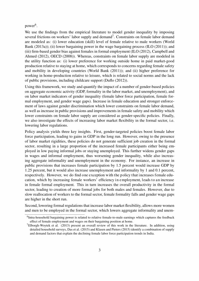
Notwithstanding rising education levels amongst women in India, female labor participationhas been declining and fell from 34 percent in 1999-00 to 27 percent in 2011-12, in both ruraland urban areas (Figure 2). Lack of decent quality jobs in the formal economy discouragefemale participation. More than 80 percent of the workforce is employed informally in India,and among the ones that are employed in the formal sector, females constitute only 19-20percent (Consensus 2011). Rigidities in the labor market due to strict regulations have beenidentified as the main drivers of this large informality1.

A considerably vast empirical literature finds a negative impact of gender inequality in em-ployment and education on economic growth2. Indeed, researchers have attempted to modelgender inequality within macroeconomic frameworks, to study the effect of a number ofgender-specific public policies on both gender and the overall economy3. However, muchof this literature has focused on how the relationship between gender and growth is mediated

1See, for instance, Besley and Burgess (2004), Sharma (2009), and ILO (2008, 2014).2See Klasen (1999), Dollar and Gatti (1999), Klasen and Lamanna (2009), and Barro and Lee (2013) among

others.3Galor and Weil (1996), Fontana (2004), Cavalcanti and Taveres (2008), Esteve-Volart (2009), Agenor (2012),

Agenor and Canuto (2013), Cuberes and Teigner (2014), and Agenor (2015).

1

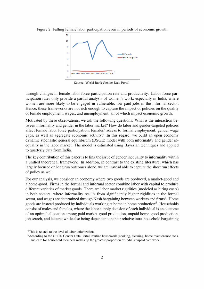
Figure 2: Falling female labor participation even in periods of economic growth

Source: World Bank Gender Data Portal

through changes in female labor force participation rate and productivity. Labor force par-ticipation rates only provide a partial analysis of women’s work, especially in India, wherewomen are more likely to be engaged in vulnerable, low paid jobs in the informal sector.Hence, these frameworks are not rich enough to capture the impact of policies on the qualityof female employment, wages, and unemployment, all of which impact economic growth.

Motivated by these observations, we ask the following questions: What is the interaction be-tween informality and gender in the labor market? How do labor and gender-targeted policiesaffect female labor force participation, females’ access to formal employment, gender wagegaps, as well as aggregate economic activity? In this regard, we build an open economydynamic stochastic general equilibrium (DSGE) model with both informality and gender in-equality in the labor market. The model is estimated using Bayesian techniques and appliedto quarterly data from India.

The key contribution of this paper is to link the issue of gender inequality to informality withina unified theoretical framework. In addition, in contrast to the existing literature, which haslargely focused on long run outcomes alone, we are instead able to capture the short run effectsof policy as well.

For our analysis, we consider an economy where two goods are produced, a market-good anda home-good. Firms in the formal and informal sector combine labor with capital to producedifferent varieties of market goods. There are labor market rigidities (modeled as hiring costs)in both sectors, where informality results from significantly higher rigidities in the formalsector, and wages are determined through Nash bargaining between workers and firms4. Homegoods are instead produced by individuals working at home in home production5. Householdsconsist of males and females, where the labor supply decision of each individual is an outcomeof an optimal allocation among paid market-good production, unpaid home-good production,job search, and leisure; while also being dependent on their relative intra-household bargaining

4This is related to the level of labor unionization.5According to the OECD Gender Data Portal, routine housework (cooking, cleaning, home maintenance etc.),

and care for household members makes up the greatest proportion of India’s unpaid care work.

2

power6.

We use the findings from the empirical literature to model gender inequality by imposingseveral frictions on workers’ labor supply and demand7. Constraints on female labor demandare modeled as: (i) lower education (skill) level of female relative to male workers (WorldBank (2013a)); (ii) lower bargaining power in the wage bargaining process (ILO (2011)); and(iii) firm-based gender bias against females in formal employment (ILO (2012), Campbell andAhmed (2012), OECD (2008)). Whereas, constraints on female labor supply are modeled inthe utility function as: (i) lower preference for working outside home in paid market-goodproduction relative to staying at home, which corresponds to concerns regarding female safetyand mobility in developing countries (World Bank (2011)); and (ii) higher preference forworking in home-production relative to leisure, which is related to social norms and the lackof public provisions, including childcare support (Duflo (2012)).

Using this framework, we study and quantify the impact of a number of gender-based policieson aggregate economic activity (GDP, formality in the labor market, and unemployment), andon labor market indicators of gender inequality (female labor force participation, female for-mal employment, and gender wage gaps). Increase in female education and stronger enforce-ment of laws against gender discrimination which lower constraints on female labor demand,as well as increase in public provisions and improvements in female safety and mobility whichlower constraints on female labor supply are considered as gender-specific policies. Finally,we also investigate the effects of increasing labor market flexibility in the formal sector, i.e.lowering labor regulations.

Policy analysis yields three key insights. First, gender-targeted policies boost female labor force participation, leading to gains in GDP in the long run. However, owing to the presence of labor market rigidities, these policies do not generate sufficient job creation in the formal sector, resulting in a large proportion of the increased female participants either being em-ployed in low paying informal jobs or staying unemployed. This further widens gender gaps in wages and informal employment, thus worsening gender inequality, while also increas-ing aggregate informality and unemployment in the economy. For instance, an increase in public provisions that increases female participation by 1.5 percent would increase GDP by 1.25 percent, but it would also increase unemployment and informality by 1 and 0.1 percent, respectively. However, we do find one exception with the policy that increases female edu-cation, which by increasing female workers’ efficiency in employment, leads to an increase in female formal employment. This in turn increases the overall productivity in the formal sector, leading to creation of more formal jobs for both males and females. However, due to slow reallocation of workers to the formal sector, female formality falls and gender wage gaps are higher in the short run.

Second, lowering formal regulations that increase labor market flexibility, allows more womenand men to be employed in the formal sector, which lowers aggregate informality and unem-

6Intra-household bargaining power is related to relative female-to-male earnings which captures the feedbackeffect of female employment and wages on their bargaining position at home.

7Elborgh-Woytek et al. (2013) present an overall review of this work in the literature. In addition, usingdetailed household surveys, Das et al. (2015) and Klasen and Pieters (2015) identify a combination of supplyand demand factors that explain the declining female labor force participation trends in India.

3

ployment in the economy boosting GDP in the long run. However, male workers gain more,as unchanged constraints on female labor supply and demand along with a positive householdincome effect, both lower female labor force participation (as opposed to increasing in theshort run and falling marginally in the long run for males) and lead to a smaller increase infemale formality in comparison to males. For instance, lower labor regulations that decreaseinformality by 1.5 percent would increase GDP by 2 percent and lower unemployment by 1.5percent, but it would also lower female participation by 0.5 percent.

Finally, we show that combining gender-targeted policies that lower constraints on female la-bor participation with reforms that boost formal job creation not only improves gender equal-ity in the labor market but also leads to significantly larger gains in GDP, employment andformality; along with minimizing any short run losses.

The remainder of this paper is organized as follows. Section 2 presents a description of theprevious literature. In Section 3 we outline the theoretical framework, and Section 4 discussesthe data, calibration and method of estimation. In Section 5, we discuss results of the esti-mation and robustness checks. Section 6 presents an analysis of several policy experiments.Section 7 concludes the paper.

2. Literature Survey

Now we turn to comparing our work with the existing theoretical policy literature on gen-der inequality. A considerably vast literature has investigated the effects of gender-specificpolicies with competitive labour markets. This literature can be broadly classified into talentallocation models (Cuberes and Teigner (2014)), occupational choice models (Esteve-Volart(2009), Hsieh et al. (2013)), overlapping generations (OLG) model (Galor and Weil (1996),Cavalcanti and Taveres (2008), Agenor and Canuto (2013), Agenor (2015)), and computablegeneral equilibrium (CGE) models (Fontana and Wood (2000), Fontana (2004), Hendy andZaki (2010)). Female labour supply in these models is often modeled using the framework ofthe time allocation model8, where women’s labour supply decision is based not only on thetrade-off between leisure and labour, but also on home production modeled as investment inchildcare. These studies analyze the impact of one or more of the following policies: increasein female education, increase in childcare provisions, better access to infrastructure, as wellas fall in exogenously given gender wage discrimination. In sum, their results suggest thateach of the above policies increase female labour participation that has a positive impact ontheir productivity, hence leading to higher growth. One or more of the following channelsdrive these results: (i) higher female labour participation increases female employment (underthe assumption of flexible labour markets) and females’ labour income; (ii) this increase infemales’ income improves the average human capital (skill) in the economy, as females areassumed to invest more in children’s education relative to males; and (iii) higher participa-tion in turn has a direct effect on per capita GDP, as females move from unpaid home-goodproduction (not accounted for in GDP) into market-good production.

8Refer to Becker (1965).

4

However, this existing literature has not paid attention to how the presence and effects oflabour market rigidities (i.e. regulations) vary by gender. In addition, much of the aboveanalysis is based on small, illustrative models (with notable exceptions such as Agenor (2012,2015)). Thus, they may not be adequate for policy analysis as important channels are ’notmodeled’ or ’shut down’ - by imposing for instance exogenously given wages, exogenouslygiven wage gaps in gender, in addition to assuming labour market flexibility. Hence, whilethis literature has significantly improved our understanding of the various links between gen-der equality and growth, the relevance of any policy-related study strongly depends on whetherthe specific model used to draw recommendations captures all the key transmission channelsof policy or not. Moreover, the computable general equilibrium (CGE) modelling technique9

is commonly used to capture the general equilibrium effects of gender-specific policies. Com-pared with the more recent general equilibrium modelling strategies, CGE models are mainlynon-stochastic and static. Thus, while they are useful for quantifying the long run effects ofreforms, they do not take into account the dynamic impact and the interplay between macroe-conomic policies and gender inequality.

We are only aware of one recent study by Albanesi and Patterson (2014) who model genderdifferences in labour force participation rates within a New Keynesian framework. How-ever, they abstract from analysing gender-specific policies and instead focus on the impact ofchanges in female labour force participation on business cycles. Although the goal of theirstudy is different to ours, they do highlight the relevance of using a DSGE framework forgender-related policy study.

Our model builds on their framework by adding a number of relevant frictions on the labour supply and demand of female workers, and by integrating this with the literature on labour market rigidities to model informality10.

3. The Model

This section presents the Baseline model. We provide a brief description before specifying thedetails of the model in the following subsections.

The small open economy consists of households, wholesale producers, retailers, capital pro-ducers, and a government. Two goods are produced in the economy: market-good and ahome-good. Market-good consist of formal tradable goods (F), informal non-tradable goods(I), and imported goods ( f ∗). The first two are produced domestically by formal and infor-mal retailers in each sector sε(F, I), respectively, while the latter is produced in the foreigneconomy and sold domestically by import retailers in the formal sector. On the other hand,home goods (H0) are produced by individuals of the household who work at home, and is forhousehold consumption only.

9CGE modeling (also referred to as Applied General Equilibrium (AGE) models), use actual data to estimatethe impact of policy changes using input-output tables.

10This literature on informality includes Conesa et al. (2002), Zenou (2008), Castillo and Montoro (2008), andSatchi and Temple (2010).

5

Households consist of male (m) and female ( f ) members who derive utility from consumingmarket goods, home goods, and leisure. Each member either supplies labor (i.e. participate inthe labor market) to wholesale firms or instead stays at home. The ones that participate in thelabor market are either employed in the formal sector, employed in the informal sector, or stayunemployed. The employed engage in paid market-good production, whereas the unemployedwork in unpaid home-good production in the residual time when unoccupied by job search.On the other hand, the ones that stay at home, are either working in home-good production, orconsuming leisure.

Formal and informal wholesale firms combine labor with capital to produce formal and infor-mal wholesale goods, respectively. Unemployment exists as wholesalers in each sector pay ahiring cost when hiring new labor a la Blanchard and Gali (2006). Wages in each sector aredetermined through Nash bargaining between workers and firms.

Formal and informal retailers purchase wholesale goods from wholesalers, differentiate theseinto different varieties of market-goods, and set the retail price for each individual variety in anenvironment of monopolistic competition and price adjustment costs a la Rotemberg (1982).A group of competitive capital producers combine formal market- and imported goods toproduce final investment goods, which is then combined with the used capital goods rentedfrom wholesalers to produce new capital. Government conducts monetary and fiscal policy:it sets the nominal interest rate using a Taylor-type rule, and receives tax wage income fromhouseholds which is used to finance public spending and unemployment benefit payments.

Details regarding each agent’s behaviour are described below.

3.1. The Labor Market

There are a continuum of households (0,1), out of which pm proportion are males, and p f =1− pm proportion are females11. Households either supply their labor to wholesale firms,which determines the labor market participation rate, or stay at home forming the pool ofnon-participants.

Hence, there are two types of workers hε(m, f ) in the labor market where m denotes maleworkers and f denotes female workers. They can either be employed in one of the two sectorssε(F, I), where F is the formal sector and I is the informal sector, or stay unemployed. Themass of male workers who are employed in the formal sector, employed in the informal sector,and unemployed, are denoted by Lm

F,t , LmI,t , and Um

t . Similarly, the mass of female workers are

denoted by L fF,t , L f

I,t , and U ft . Non-participants consist of NPm

t males and NP ft females.

The pool of male and female workers who participate in the labor market is then given by:Pm

t = pm−NPmt and P f

t = p f −NP ft , whereas the male and female unemployment is deter-

mined by: Umt =Pm

t −LmF,t−Lm

I,t and U ft =P f

t −L fF,t−L f

I,t , respectively. Hence, we can expressunemployment as:

11As per the 2001 consensus, females in India constitutes half of the country’s population and therefore weassume pm = p f = 1

2 .

6

Umt = pm−NPm

t −LmF,t−Lm

I,t (3.1)

U ft = p f −NP f

t −L fF,t−L f

I,t (3.2)

The labor market dynamics closely follow the framework in Campolmi and Gnochhi (2014).The stock of employed labor varies because of the endogenous variation in hiring, and anexogenous probability of getting fired, σs, every period12. At the end of period t − 1, afterall decisions have been taken and executed, Fm

s,t−1 = σms Lm

s,t−1 and F fs,t−1 = σ

fs L f

s,t−1 male andfemale workers are fired by wholesalers in sector s. In period t, new male and female workersare hired, Hm

s,t and H fs,t , from the pool of job searchers, Sm

t and S ft

13. The evolution of maleand female labor in each sector s is given by:

Lms,t = Lm

s,t−1−Fms,t−1 +Hm

s,t = (1−σs)Lms,t−1 + p(Hm

s,t)Smt (3.3)

L fs,t = L f

s,t−1−F fs,t−1 +H f

s,t = (1−σs)Lfs,t−1 + p(H f

s,t)Sft (3.4)

where male and female workers’ probability of getting hired, p(Hms,t) and p(H f

s,t), is deter-mined endogenously by wholesalers’ optimization14.

The unemployed, the non-participants, and fired individuals, Umt−1 +NPm

t−1 +FmF,t−1 +Fm

I,t−1

and U ft−1 +NP f

t−1 +F fF,t−1 +F f

I,t−1, form the pool of males and females that are not employedat the end of period t−1. Among these, some are job searchers in the following period t, andthe remaining ones are non-participants:

Smt +NPm

t =Umt−1 +NPm

t−1 +σmF Lm

F,t−1 +σmI Lm

I,t−1 (3.5)

S ft +NP f

t =U ft−1 +NP f

t−1 +σf

F L fF,t−1 +σ

fI L f

I,t−1 (3.6)

Inserting Eq. 3.1 in Eq. 3.5, and Eq. 3.2 in Eq. 3.6, gives us the following expressions formale and female job searchers in period t:

Smt = Pm

t − (1−σF)LmF,t−1− (1−σI)Lm

I,t−1 (3.7)

S ft = P f

t − (1−σF)LfF,t−1− (1−σI)L

fI,t−1 (3.8)

12Probability of getting fired is allowed to vary across the two sectors, which corresponds to the relative difficultyin firing workers in the formal sector (i.e. employment protection policies).

13Assume instantaneous hiring, i.e. period t searchers can be matched and start producing in period t itself. Thisis a standard assumption in a sticky-price model, and seems reasonable if a period is interpreted as a quarter.

14The formal and informal labor markets are integrated as they hire workers from the same pool of male andfemale job searchers.

7

Evolution of male and female formal employment (Eq. 3.3 and Eq. 3.4 with s = F) can thenbe written as:

LmF,t = (1−σF)(1− p(Hm

F,t))LmF,t−1 + p(Hm

F,t)Pmt − p(Hm

F,t)(1−σI)LmI,t−1 (3.9)

L fF,t = (1−σF)(1− p(H f

F,t))LfF,t−1 + p(H f

F,t)Pf

t − p(H fF,t)(1−σI)L

fI,t−1 (3.10)

Eq. 3.10 implies that in period t, total female workers employed in the formal sector increaseswith higher female labor participation, P f

t , and with a rise in their probability of getting hiredin this sector, p(H f

F,t)15. An analogous interpretation of Eq. 3.9 follows for male workers

employed in the formal sector.

Similarly, for the informal sector (s = I), we get:

LmI,t = (1−σI)(1− p(Hm

I,t))LmI,t−1 + p(Hm

I,t)Pmt − p(Hm

I,t)(1−σF)LmF,t−1 (3.11)

L fI,t = (1−σI)(1− p(H f

I,t))LfI,t−1 + p(H f

I,t)Pf

t − p(H fI,t)(1−σF)L

fF,t−1 (3.12)

Probability of getting hired in sector s is then given by the ratio of new hires to the pool of jobsearchers:

p(Hms,t) =

Hms,t

Smt

p(H fs,t) =

H fs,t

S ft

(3.13)

Ratio of total job searchers to the pool of individuals not employed at the end of period t−1determines the probability of searching for a job:

p(Smt ) =

Smt

Umt−1 +NPm

t−1 +FmF,t−1 +Fm

I,t−1(3.14)

p(S ft ) =

S ft

U ft−1 +NP f

t−1 +F fF,t−1 +F f

I,t−1

(3.15)

3.2. Wholesale Producer

We have a continuum of wholesalers (0,1) in each sector s producing different intermediategoods, YW

F,t and YWI,t , with access to different technologies, θF,t and θI,t

16. By the beginningof period t, they are assumed to acquire capital, KF,t−1 and KI,t−1, from capital producers,

15For this to hold, female labor participation in period t should be greater than the sum of female workers thatare still employed from the previous period t − 1, i.e. P f

t > (1−σF)LfF,t−1 +(1−σI)L

fI,t−1. This always

holds true for all periods in our model.16θF,t and θI,t are stochastic disturbances to aggregate productivity in the formal and informal sector, respectively

and follow a first order autoregressive process (AR(1)) in logs.

8

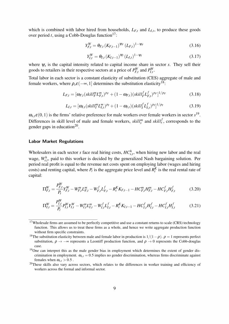
which is combined with labor hired from households, LF,t and LI,t , to produce these goodsover period t, using a Cobb-Douglas function17:

YWF,t = θF,t (KF,t−1)

ψF (LF,t)1−ψF (3.16)

YWI,t = θI,t (KI,t−1)

ψI (LI,t)1−ψI (3.17)

where ψs is the capital intensity related to capital income share in sector s. They sell theirgoods to retailers in their respective sectors at a price of PW

F,t and PWI,t .

Total labor in each sector is a constant elasticity of substitution (CES) aggregate of male andfemale workers, where ρsε(−∞,1] determines the substitution elasticity18:

LF,t = [ωF,t(skillmF Lm

F,t)pF +(1−ωF,t)(skill f

FL fF,t)

pF ]1/pF (3.18)

LI,t = [ωI,t(skillmI Lm

I,t)pI +(1−ωI,t)(skill f

I L fI,t)

pI ]1/pI (3.19)

ωs,tε(0,1) is the firms’ relative preference for male workers over female workers in sector s19.Differences in skill level of male and female workers, skillm

s and skill fs , corresponds to the

gender gaps in education20.

Labor Market Regulations

Wholesalers in each sector s face real hiring costs, HChs,t , when hiring new labor and the real

wage, W hs,t , paid to this worker is decided by the generalized Nash bargaining solution. Per

period real profit is equal to the revenue net costs spent on employing labor (wages and hiringcosts) and renting capital, where Pt is the aggregate price level and RK

t is the real rental rate ofcapital:

ΠWF,t =

PWF,t

PtYW

F,t−W mF,tL

mF,t−W f

F,tLfF,t−RK

t KF,t−1−HCmF,tH

mF,t−HC f

F,tHf

F,t (3.20)

ΠWI,t =

PWI,t

PtPW

I,t YWI,t −W m

I,tLmI,t−W f

I,tLfI,t−RK

t KI,t−1−HC fI,tH

fI,t−HC f

I,tHf

I,t (3.21)

17Wholesale firms are assumed to be perfectly competitive and use a constant returns to scale (CRS) technologyfunction. This allows us to treat these firms as a whole, and hence we write aggregate production functionwithout firm specific constraints.

18The substitution elasticity between male and female labor in production is 1/(1−ρ). ρ = 1 represents perfectsubstitution, ρ → −∞ represents a Leontiff production function, and ρ → 0 represents the Cobb-douglascase.

19One can interpret this as the male gender bias in employment which determines the extent of gender dis-crimination in employment. ωs,t = 0.5 implies no gender discrimination, whereas firms discriminate againstfemales when ωs,t > 0.5 .

20These skills also vary across sectors, which relates to the differences in worker training and efficiency ofworkers across the formal and informal sector.

9

Following Blanchard and Gali (2006), hiring costs depend positively on the total number ofnew hires, and negatively on the pool of unemployed at the beginning of period t21:

HChF,t =

(βHCF ,t

)(p(Hh

F,t))

αHCF (3.22)

HChI,t =

(βHCI,t

)(p(Hh

I,t))

αHCI (3.23)

βHCF,t,βHCI,t > 0 are exogenous AR(1) hiring cost shocks, and αHCs > 0 is the elasticity ofhiring cost with respect to hiring probability22.

Capital and Labor Demand

Wholesalers in sector s choose Lms,t , L f

s,t , Hms,t , H f

s,t , and Ks,t−1, by maximising their expecteddiscounted value of future profits:

maxLs,t ,Ks,t−1,Hs,t

Et

∞

∑k=0

ρt,t+kΠWs,t+k (3.24)

subject to the law of motion of male and female employment (Eq. 3.3 and Eq. 3.4). ρt,t+kis the stochastic discount rate obtained from the households’ optimization problem discussedbelow.

Capital and labor demand functions in sector s are obtained from the first order conditions asfollows (see Technical Appendix for derivations):

RKt = ψs

PWs,t

Pt

YWs,t

Ks,t−1(3.25)

(1−ψs)ωsPW

s,t

Pt

YWs,t

Lms,t

(skillm

sLm

s,t

Ls,t

)ρs

=W ms,t +HCm

s,t−Et(ρt,t+1HCm

s,t+1(1−σs))

(3.26)

(1−ψs)(1−ωs)PW

s,t

Pt

YWs,t

L fs,t

(skill f

sL f

s,t

Ls,t

)ρs =W f

s,t +HC fs,t−Et

(ρt,t+1HC f

s,t+1(1−σs))

(3.27)

The equation for capital demand (Eq. 3.25) is standard in the literature, however, the labor de-mand for males and females (Eq. 3.26 and Eq. 3.27) is now determined by equating marginalproduct to the marginal cost of employing labor, which includes the real wage plus the costgenerated by hiring.

21Blanchard and Gali (2006) show that the presence of hiring costs creates a friction in the labor market similarto the cost of posting a vacancy and the time needed to fill it in the standard Diamond-Mortenssen-Pissaridis(DMP) model.

22This points towards a convex structure of hiring costs, i.e. marginal hiring costs increase with the number ofnew hires.

10

Wage Bargaining

Wage setting follows a Nash bargaining process between workers and wholesalers where wagebargaining power of worker h in the formal and informal sector is denoted by λ h

Fε(0,1) andλ h

I ε(0,1), respectively. The bargaining power of formal workers is assumed to to be higherthan informal workers. To capture gender gaps in access to labor unions, union leadership,and union priorities, we also allow for differences in bargaining power of male and femaleworkers.

V hF,t , V h

I,t , and V hU,t is the marginal value to a worker h of being employed formally, employed

informally, and of being unemployed, whereas V hNP,t is the value of not participating in the

labor market. A formally employed worker in period t receives current wage income of(1− τF)WF,t , where τF is the marginal tax rate. In the next period t + 1, the worker keepsthe same job with probability (1−σh

F), or gets fired with probability σhF . If fired, there is

a probability (1− p(ShF,t+1)) that the worker decides to stay at home, or searches for jobs

with probability p(ShF,t+1). If the worker searches for jobs, there is a probability p(Hh

F,t+1) ofgetting re-hired in the same sector, hired in the informal sector p(Hh

I,t+1), and a probability1−∑s=F,I(p(Hh

s,t+1))ds of staying unemployed. Hence, we obtain the following expressionfor V h

F,t :

V hF,t = (1− τF)W h

F,t−MRShHPt ,Ct

−MRShlet ,Ct

+Et

[ρt,t+1(1−σ

hF)V

hF,t+1

]+σ

hFEt

{ρt,t+1 p(Sh

t+1)[(p(Hh

F,t+1)VhF,t+1 + p(Hh

I,t+1)VhI,t+1

]}(3.28)

+σhFEt

[ρt,t+1(1− p(Hh

F,t+1)− p(HhI,t+1))V

hU,t+1

]+σ

hFEt

[ρt,t+1(1− p(Sh

t+1))VhNP,t+1

]MRSh

HPt ,Ctand MRSh

let ,Ct, both derived from the households optimization problem below, rep-

resent the marginal rate of substitution between home-good and market-good consumption,and between leisure and market-good consumption

Similarly, we get the value of being employed in the informal sector, the only difference beingthat the worker does not pay wage income tax, τI = 0:

V hI,t = (1− τI)W h

I,t−MRShHPt ,Ct

−MRShlet ,Ct

+Et

[ρt,t+1(1−σ

hI )V

hI,t+1

]+σ

hI Et

{ρt,t+1 p(Sh

t+1)[(p(Hh

F,t+1)VhF,t+1 + p(Hh

I,t+1)VhI,t+1

]}(3.29)

+σhI Et

[ρt,t+1(1− p(Hh

F,t+1)− p(HhI,t+1))V

hU,t+1

]+σ

hI Et

[ρt,t+1(1− p(Sh

t+1))VhNP,t+1

]An unemployed worker receives social benefits today, WU,t , and spends τU ε(0,1) proportionof her time in home-good production, while the remaining time (1− τU) is spent in searching

11

for jobs23. In the next period, there is a probability p(Sht+1) that the worker stays at home or

participates in the labor market with probability (1− p(Sht+1)), which gives us the expression

for V hU,t as follows:

V hU,t =WU,t− (1− τU)MRSh

HPt ,Ct−MRSh

let ,Ct(3.30)

+Etρt,t+1

{ρt,t+1 p(Sh

t+1)[(p(Hh

F,t+1)VhF,t+1 + p(Hh

I,t+1)VhI,t+1

]}+Et

[ρt,t+1(1− p(Hh

F,t+1)− p(HhI,t+1))V

hU,t+1

]+Et

[ρt,t+1(1− p(Sh

t+1))VhNP,t+1

]A non-participant household member, either works in home-good production with probability(1− p(leh

t+1)), or consumes leisure with probability p(leht+1)

24. This gives us the marginalvalue to worker h of not participating (i.e. staying at home) as:

V hNP,t+1 = (1− p(leh

t+1))VhHP,t+1 + p(leh

t+1)Vhle,t+1 (3.31)

Value of working in home-good production, V hHP,t+1 and value of consuming leisure, V h

le,t+1,are analogous to the value of being unemployed, except that these workers are now not entitledto receive unemployment benefits25:

V hHP,t =−MRSh

let ,Ct(3.32)

+Etρt,t+1

{ρt,t+1 p(Sh

t+1)[(p(Hh

F,t+1)VhF,t+1 + p(Hh

I,t+1)VhI,t+1

]}+Et

[ρt,t+1(1− p(Hh

F,t+1)− p(HhI,t+1))V

hU,t+1

]+Et

[ρt,t+1(1− p(Sh

t+1))VhNP,t+1

]

V hle,t =−MRSh

HPt ,Ct(3.33)

+Etρt,t+1

{ρt,t+1 p(Sh

t+1)[(p(Hh

F,t+1)VhF,t+1 + p(Hh

I,t+1)VhI,t+1

]}+Et

[ρt,t+1(1− p(Hh

F,t+1)− p(HhI,t+1))V

hU,t+1

]+Et

[ρt,t+1(1− p(Sh

t+1))VhNP,t+1

]23We assume a unit interval for the time period.24These probabilities are endogenously determined by households optimization25In the context of India, the unemployment benefits could be thought of as the benefits under the scheme of the

Mahatama Gandhi National Rural Employment Guarantee Act (MNREGA). The stated objective of the Act is“to enhance livelihood security in rural areas by providing at least 100 days of guaranteed wage employmentin a financial year to every household whose adult members volunteer to do unskilled manual labor”.

12

An unemployed worker h has a utility gain of(

V hF,t−V h

U,t

)if hired in the formal sector and a

gain of(

V hI,t−V h

U,t

)if hired in the informal sector.

Following the derivations in Blanchard and Gali (2006), sector s wholesalers’ value of hiringan additional worker h in period t, Jh

s,t , is simply given by the hiring cost in the same period,i.e Jh

s,t = HChs,t

26. Generalized Nash bargaining over the wage rate determines the division ofrent between worker h and wholesaler in sector s:

maxW h

s,t

(V h

s,t−V hU,t

)λ hs,t

Jhs,t

(1−λ hs,t)

and the equation determining wages, W hs,t , is:

V hs,t−V h

U,t =λ h

s,t

1−λ hs,t(1− τs)Jh

s,t (3.34)

We derive the expressions for wage rate of male and female workers in the Techinacal Ap-pendix and define average male and female wages, W m

t and W ft , by the ratio of total after tax

wage income divided by the total number of individuals employed:

W mt =

W mF,tL

mF,t(1− τF)+W m

I,tLmI,t

LmF,t +Lm

I,tW f

t =W f

F,tLfF,t(1− τF)+W f

I,tLfI,t

L fF,t +L f

I,t

where ratio of average male wages to average female wages, W mt

W ft

, is defined as the ’gender

wage gap’.

3.3. Retailers

A continuum jF and jI of monopolistically competitive formal and informal retailers buywholesale goods to produce different final market-good varieties, YF,t( jF) and YI,t( jI), andsell these at different prices, PF,t( jF) and PI,t( jI), respectively27.

Total composite output in each sector s, Ys,t , produced by retailers is a Dixit-Stiglitz (1977)CES aggregate of different varieties of goods produced by individual retailers, Ys,t( js).

Ys,t =

1ˆ

0

Ys,t ( js)εs−1

εs d js

εs

εs−1

(3.35)

26This is because in our framework there is no search time for hiring new worker (i.e. instant hiring assumption),and so a firm can always replace a worker who is fired at this cost.

27We assume zero cost of differentiation.

13

εs stands for the elasticity of substitution between different varieties of goods. The corre-sponding price of the composite consumption good, Ps,t is:

Ps,t =

1ˆ

0

Ps,t ( js)1−εsd js

1

1−εs

(3.36)

The demand function facing each retailer can be written as:

Ys,t( js) =(

Ps,t( js)Ps,t

)−εs

Ys,t (3.37)

Formal final good, YF,t , is exportable where it is consumed both domestically QdF,t , by house-

holds, capital producers and government, and is also exported Qxt to the rest of the world. On

the other hand, the informal sector good YI,t is nontradable and is only consumed domesticallyby households, Qd

I,t .

Price Setting

Retailer js sets its price, Ps,t( js) that maximizes its expected discounted stream of future prof-its:

MaxPs,t( js)

Et

∞

∑k=0

ρt,t+kΠRt,t+k( js) (3.38)

where the one-period profit in the formal sector, ΠRF,t( jF), is given by the sum of total revenues

from its domestic demand,(

PF,t( jF )PF,t

)−εFQd

F,t and export demand(

PF,t( jF )PF,t

)−εFQx

t , net of thecosts of price adjustment. Per-period profits are then obtained as:

ΠRF,t( jF) =

(PF,t ( jF)

Pt−MCW

F,t

)(PF,t ( jF)

PF,t

)−εF

(QdF,t +Qx

t ) (3.39)

−φ

ad jF2

(PF,t ( jF)/PF,t−1 ( jF)

π−1)2

(QdF,t +Qx

t )

Here MCWF,t is the real marginal cost, which is equal to the perfectly competitive wholesalers’

real pricePW

F,tPt

. Aggregate price and formal price inflation are given by πt =Pt

Pt−1and πF,t =

PF,tPF,t−1

, where π is the steady state economy wide inflation28. Following Rotemberg (1982),

we have quadratic costs of price adjustment φad jF2

(PF,t( jF )/PF,t−1( jF )

π−1)2

, and φad jF ≥ 0 is a

parameter determining the degree of nominal rigidity in the formal sector.

28Variables without a time subscript t denotes their respective steady state values.

14

Per-period profits of informal retailers are similar, except that the informal sector only sells itsgoods domestically:

ΠRI,t( jI) =

(PI,t ( jI)

Pt−MCW

I,t

)(PI,t ( jI)

PI,t

)−εI

QdI,t (3.40)

−φ

ad jI2

(PI,t ( jI)/PI,t−1 ( jI)

π−1)2

QdI,t

φad jI ≥ 0 determines the degree of nominal rigidity in informal prices and πI,t =

PI,tPI,t−1

is theinflation in informal prices.

The first order condition of the retailer optimization problem determines the price in eachsector s (refer to Technical Appendix):

Ps,t( js)Pt

=εs

εs−1MCW

j,t +φ

ad js

εs−1(πs,t

π−1)

πs,t

π(3.41)

−Et

{ρt,t+1

[(φ

ad js

εs−1

)(πs,t+1

π−1)(

πs,t+1

π

)Ys,t+1( js)Ys,t( js)

]}εs

εs−1 is the desired (gross) mark-up, resulting from the imperfections in the retail market.We assume that import prices follow a similar pricing rule as that of the formal goods, withφ

ad jf∗ ≥ 0 determining the degree of nominal rigidity in import prices.

3.4. Household

Utility Function

The households aggregate utility function is a weighted sum of male utility, Λmt , and female

utility, Λft , where the weights are determined by the intra-household bargaining power of

males and females:

Λt = Et

∞

∑t=0

βt[(BPt)(pm)Λm

t +(1−BPt)(p f )Λft

](3.42)

β is the nominal discount rate and BPt ε (0,1) is the endogenously determined intra-householdbargaining power of males relative to females29. Following Klaveren (2009), BPt is an in-creasing function of male to female wage income ratio given by:

BPt =

exp[(1−τF )W m

F LmF+W m

I LmI

(1−τF )Wf

F L fF+W f

I L fI

]1+ exp

[(1−τF )W m

F LmF+W m

I LmI

(1−τF )Wf

F L fF+W f

I L fI

]29The higher the value of BPt , the more the male utility function is weighted in the overall household utility.

15

Bargaining power of male increases with an increase in his own steady state wage income,whereas it decreases with a rise in the steady state wage income of females..

Each member derives utility from consuming market-produced goods Ct , home-producedgoods H0

t , and leisure leht :

Λm(Ct,H0

t , lemt ) = (1−hc)ln(Ct−hcCt−1)+φ

mt

((H0

t )1+vm

H,t

1+νmH,t

+ϕmle,t

(lemt )

1+vmle,t

1+νmle,t

)(3.43)

Λf (Ct,H0

t , left ) = (1−hc)ln(Ct−hcCt−1)+φ

ft

(H0t )

1+v fH,t

1+νf

H,t

+ϕf

le,t(le f

t )1+v f

le,t

1+νf

le,t

(3.44)

Market and home consumption are public goods, and there is risk sharing within the house-hold, so that all its members - males and females, consume the same amount of these goods.The disutility of working, on the other hand, accrues to each member individually. Therefore,males do not get any utility from female leisure and vice-versa. Ct denotes aggregate con-sumption at time t, while Ct−1 is the average level of consumption in t−1, where hc ∈ [0,1)is the external habit formation parameter. −υh

H,t is the inverse inter-temporal elasticity of sub-stitution between market-good consumption and home-good consumption, and −υh

le,t is theinverse inter-temporal elasticity of substitution between market consumption and leisure.

φ ht is an exogenously given weight each member places on their utility from consuming home

goods and leisure (i.e, utility from staying at home) relative to consuming market goods (i.e.participating in paid market work). This coefficient captures the constraints on engaging inwork outside home such as safety and mobility issues. ϕh

le determines the relative weighton utility from engaging in home-good production relative to utility from consuming leisure.This also varies across males and females, which corresponds to the deeply ingrained genderbiased social norms and lack of childcare facilities in developing countries.

Home-good Production

Home goods are produced by males and females working in home production (home workers),HPm

t and HP ft , combined with the unemployed in the labor market who engage in home-good

production in their residual time unoccupied by job search. After normalizing to one thetotal time available to each worker, the unemployed spend τU ε(0,1) proportion of their timeworking in home-good production, where (1−τU) is then the search cost. We assume a home-good production function with decreasing returns to scale, where −ρH is a coefficient of theinverse inter-temporal elasticity between male and female home workers30:

H0t = θH,t

{[(1−BPt)(HPm

t + τUUmt )pH +BPt(HP f

t + τUU ft )

pH]1/pH

}1−αH

(3.45)

θH,t is the exogenous AR(1) shock to home productivity31. Intra-household bargaining power,BPt , determines the weight on female relative to male workers in home-good production,30Christiano et al. (2014) use a similar home production function in their framework.31This corresponds to public provisions and infrastructure such as sanitation, access to water and electricity.

16

where higher the bargaining power of males at home, i.e. higher BPt , lower is the weighton male workers in home production.

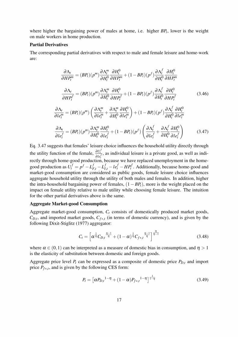
Partial Derivatives

The corresponding partial derivatives with respect to male and female leisure and home-workare:

∂Λt

∂HPmt

= (BPt)(pm)∂Λm

t

∂H0t

∂H0t

∂HPmt+(1−BPt)(p f )

∂Λft

∂H0t

∂H0t

∂HPmt

∂Λt

∂HP ft= (BPt)(pm)

∂Λmt

∂H0t

∂H0t

∂HP ft+(1−BPt)(p f )

∂Λft

∂H0t

∂H0t

∂HP ft

(3.46)

∂Λt

∂ lemt= (BPt)(pm)

(∂Λm

t∂ lem

t+

∂Λmt

∂H0t

∂H0t

∂ lemt

)+(1−BPt)(p f )

∂Λft

∂H0t

∂H0t

∂ lemt

∂Λt

∂ le ft= (BPt)(pm)

∂Λmt

∂H0t

∂H0t

∂ le ft+(1−BPt)(p f )

(∂Λ

ft

∂ le ft+

∂Λft

∂H0t

∂H0t

∂ le ft

)(3.47)

Eq. 3.47 suggests that females’ leisure choice influences the household utility directly through

the utility function of the female, ∂U ft

∂ le ft, as individual leisure is a private good, as well as indi-

rectly through home-good production, because we have replaced unemployment in the home-good production as U f

t = p f −L fF,t −L f

I,t − le ft −HP f

t . Additionally, because home-good andmarket-good consumption are considered as public goods, female leisure choice influencesaggregate household utility through the utility of both males and females. In addition, higherthe intra-household bargaining power of females, (1−BPt), more is the weight placed on theimpact on female utility relative to male utility while choosing female leisure. The intuitionfor the other partial derivatives above is the same.

Aggregate Market-good Consumption

Aggregate market-good consumption, Ct consists of domestically produced market goods,CD,t , and imported market goods, C f∗,t (in terms of domestic currency), and is given by thefollowing Dixit-Stiglitz (1977) aggregator:

Ct =[α

1η CD,t

η−1η +(1−α)

1η C f∗,t

η−1η

] η

η−1(3.48)

where α ∈ (0,1) can be interpreted as a measure of domestic bias in consumption, and η > 1is the elasticity of substitution between domestic and foreign goods.

Aggregate price level Pt can be expressed as a composite of domestic price PD,t and importprice Pf∗,t , and is given by the following CES form:

Pt =[αPD,t

1−η +(1−α)Pf∗,t1−η] 1

1−η (3.49)

17

Domestic market-good consumption is a composite of formal market-good consumption, CF,t ,and informal market-good consumption, CI,t expressed as:

CD,t =

[w

1µ C

µ−1µ

F,t +(1−w)1µ C

µ−1µ

I,t

]µ

µ−1 (3.50)

where wε (0,1) is the weight on formal sector market-good, and µ > 1 is the elasticity ofsubstitution between the goods produced in the two sectors. Then, aggregate domestic market-good price, PD,t , is determined by:

PD,t =[wP1−µ

F,t +(1−w)P1−µ

I,t

] 11−µ (3.51)

By minimizing household expenditure on the total composite demand, we can derive the fol-lowing optimal consumption demand functions for aggregate domestic and imported marketgoods:

CD,t = α

(PD,t

Pt

)−ηCt C f∗,t = (1−α)

(Pf∗,t

Pt

)−ηCt (3.52)

Similarly, we derive the optimal consumption demand functions for domestically producedformal and informal market-goods:

CF,t = w(

PF,t

PD,t

)−µCD,t CI,t = (1−w)

(PI,t

PD,t

)−µCD,t (3.53)

Budget ConstraintThe representative household enters period t with one period (real) foreign and domesticbonds, B∗t−1(in foreign currency) and Dt−1, both of which yield a nominal interest rate ofi ft−1 and it−1 over the period t, respectively. In addition, during period t, individuals who are

employed, earn after tax wage income of(

∑h=m, f

[(1− τF)W h

F,tLhF,t

]dh)

in formal jobs and(∑h=m, f

[(1− τI)W h

I,tLhI,t

]dh)

in informal jobs, and the unemployed receive social benefits,

(WU,t)(Umt +U f

t ). They receive real dividends arising from the ownership of the retail firms,ΠR

F,t and ΠRI,t . The income is spent on the consumption of market goods, Ct , and the purchase

of one period bonds for the subsequent period, B∗t and Dt . Denoting et as the nominal ex-change rate where an increase in its value implies depreciation of domestic currency, we havethe following period budget constraint of the household in real terms, with RERt =

etP∗tPt

as thereal exchange rate::

Ct +RERtB∗t +Dt (3.54)

=

(et

et−1

)(1+ i f

t−1

πt

)(RERt−1)B∗t−1 +

(1+ it−1

πt

)Dt−1

+(1− τF)W mF,tL

mF,t +(1− τF)W

fF,tL

fF,t +W m

I,tLmI,t +W f

I,tLfI,t

+WU,t(Umt +U f

t )+ΠRF,t +Π

RI,t

18

The resulting first order conditions with respect to Ct , Bt , and Dt yield the standard Eulerequation for consumption (see Technical Appendix):

1 = βEt

{(Ct−hCCt−1

Ct+1−hCCt

)(1+ itπt+1

)}(3.55)

1 = βEt

{(Ct−hCCt−1

Ct+1−hCCt

)(1+ i f

t

πt+1

)(et+1

et

)}(3.56)

Combining Eq. 3.55 and Eq. 3.56 (up to a log-linear approximation) gives us the uncovered

interest rate parity (UIP) condition(

1+itπt+1

)=

(1+i f

tπt+1

)(et+1et

).

The remaining first order conditions for HPmt ,HP f

t , lemt , and le f

t yield the labor supply equa-tion32:

MRShHPt ,Ct

= (1− τF)W hF,t p(Hh

F,t)+W hI,t p(Hh

I,t) (3.57)

+WU,t

[1− p(Hh

F,t)− p(HhI,t)]

MRShlet ,Ct

= (1− τF)W mF,t p(Hm

F,t)+W mI,t p(Hm

I,t) (3.58)

+WU,t[1− p(Hm

F,t)− p(HmI,t)]

Finally, probability that a non-participant household member h consumes leisure, p(leht ), is

given by the ratio of the ones consuming leisure divided by the individuals who stay at home:

p(leht ) =

leht

HPht + leh

t≡ leh

t

NPht

where(1− p(leh

t ))

is then the probability that a non-participant household member h engagesin home-production.

3.5. Capital Producer

Capital producers combine the existing undepreciated capital stock, (1−δK)Kt−1, leased fromwholesalers, with investment goods, It , to produce new capital Kt , using a linear technology.The capital-producing sector is perfectly competitive. Capital evolves according to the fol-lowing equation:

Kt = (1−δK)Kt−1 +PInv

tPt

It−κ

2

(PInv

tPt

ItKt−1

−δK

)2

Kt−1 (3.59)

32The expressions for MRShHPt ,Ct

=(

∂Λt∂HPh

t

)/(

∂Λt∂Ct

)and MRSh

let ,Ct=

(∂Λt

∂ le ft

)/(

∂Λt∂Ct

)are derived in the Techni-

cal Appendix.

19

where κ

2

(PInv

tPt

ItKt−1−δK

)2Kt−1 is the capital adjustment cost. Here κ ≥ 0 is the capital adjust-

ment coefficient, and δK is the depreciation rate of physical capital.

Capital production is confined to the formal sector, and investment is thus a composite ofdomestic formal goods and foreign imports:

It =[α

1η IF,t

η−1η +(1−α)

1η I f∗,t

η−1η

] η

η−1(3.60)

and the price of investment is:

PInvt =

[αPF,t

1−η +(1−α)Pf∗,t1−η] 1

1−η (3.61)

We assume that it is in the same proportion as in the consumption basket (Eq. 3.52 and Eq.3.53), except that now weight on formal good is w = 1. Hence, optimal demand for domesticand imported investment goods is:

IF,t = α

(PF,t

PInvt

)−η It I f ∗,t = (1−α)

(Pf∗,tPInv

t

)−η It

The capital producer invests such that its profit is maximized, where Qt is the real price ofcapital:

maxIt

Qt

(PInv

tPt

It−κ

2

(PInv

tPt

ItKt−1

−δK

)2

Kt−1

)− PInv

tPt

It

The corresponding first order condition w.r.t. to the choice of It determines the capital supplyequation (see Technical Appendix):

Qt

[1−κ

(PInv

tPt

ItKt−1

−δK

)]= 1 (3.62)

This is the Tobin’s (1969) Q equation relating the price of capital to marginal adjustment costs.In the absence of capital adjustment costs (κ = 0), the price of capital is constant and equal toone.

Demand for capital by wholesalers in sector s must satisfy the following condition:

Et (Rt+1Qt) = Et

{ψF

(PW

s,t+1

Pt+1

)(YW

s,t+1

Ks,t

)+(1−δK)Qt+1

}

20

3.6. Rest of the World

Foreign economy consumes domestic formal exports, Qxt , supplies foreign goods to domestic

country as imports, Qmt , and sells foreign bonds, B∗t to domestic households. We assume

that the domestic economy is small, which implies that it cannot affect foreign output, Y ∗t ,foreign inflation, π∗t =

P∗tP∗t−1

, and the foreign interest rate, i∗t , all of which are assumed to be

exogenously determined in the rest of the world33.

The demand for domestic exports by the foreign economy is assumed to have a similar struc-ture to that of domestic consumption in Eq. 3.52:

Qxt = α

∗x (

P∗X ,t

P∗t)−η∗x Y ∗t (3.63)

where α∗x ε(0,1) is a parameter determining the share of domestic goods in foreign consump-tion bundle, and η∗x > 1 is the substitution elasticity between exports and foreign domesticgoods. We assume that law of one price (LOOP) holds for domestic goods, allowing us toexpress the price of exports in foreign currency as P∗X ,t =

PF,tet

34.

Following Schmitt-Grohe and Uribe (2003), interest rate on foreign bond, i ft , depends not only

on the exogenous foreign interest rate, i∗t , but also on the foreign currency borrowing premium,χ , whereby holders of foreign debt are assumed to face an interest rate that is increasing in thecountry’s net foreign debt:

(1+ i ft ) = (1+ i∗t )−χ

(B∗t −B∗

PF(RER)PQx

)(3.64)

This is a standard assumption in the small open economy literature35.

3.7. Government Policy

Government consists of monetary and fiscal authorities. The monetary authority sets the nom-inal interest rate, it , based on a Taylor-type (1993) feedback rule. It responds to deviations ininflation and gross domestic product:

iti=

(it−1

i

)αi(

πt

π

)απ

(Yt

Y

)αY εi,t (3.65)

where αi captures interest rate smoothing, and the Taylor rule coefficients, απ and αY , are therelative weights on inflation and output stabilization respectively. i, π , and Y are the steady33We normalise the value of foreign output by assuming Y ∗t = 1.34Substituting the LOOP condition, and RERt =

et P∗tPt

in Eq. 3.63, we get the following Qxt = α∗x (

PF,tPt

1RERt

)−η∗x Y ∗t .Therefore, a real depreciation of the currency increases exports.

35The need for such a friction is mainly technical, i.e. the country borrowing premium ensures that the modelhas a unique steady state and ensures stationarity.

21

state values for nominal interest rate, inflation, and gross domestic product. εi,t is a monetarypolicy shock to capture unanticipated changes in the nominal interest rate.

In addition, the fiscal authority finances its consumption, Gt , and unemployment benefit pay-ments by taxing wage income in the formal sector36. The government budget constraint everyperiod is:

PInvtPt

Gt +WU,t(Umt +U f

t ) = τF(W mF,tL

mF,t +W f

F,tLfF,t) (3.66)

We assume that exogenously given government consumption basket, Gt , analogous to theinvestment basket in Eq. 3.60, consists of domestic formal market goods, GF,t , along withforeign imports, G f∗,t (in domestic currency):

Gt =[α

1η GF,t

η−1η +(1−α)

1η G f∗,t

η−1η

] η

η−1(3.67)

Optimal demand for domestic formal, GF,t , and imported government consumption, G f ∗,t , isgiven by:

GF,t = α

(PF,t

PInvt

)−ηGt G f∗,t = (1−α)

(Pf ∗,t

PInvt

)−ηGt

3.8. Market Clearing and Aggregation

Sum of employment in the formal, LF,t , and in the sector, LI,t , is equal to aggregate employ-ment Lt in the economy: LF,t +LI,t = Lt . Aggregate labor force participation in the economy(i.e. aggregate labor supply in the economy), Pt is a sum of the male and female labor par-ticipation: Pt = Pm

t +P ft

37. Aggregate unemployment can then be written as aggregate laborsupply, Pt minus aggregate employment, Lt : Ut = Pt − Lt , where the unemployment rate isobtained by dividing through by the total number of labor market participants, Pt .

Equilibrium in the labor market for males and females is given by equating aggregate supplyof male and female labor, Pm

t and P ft , to the sum of their respective demands by formal and

informal wholesalers, plus the ones unemployed:

Pmt = Lm

F,t +LmI,t +Um

t P ft = L f

F,t +L fI,t +U f

t

Male and female unemployment is given by the ones searching for a job minus the ones thatget hired:

Umt = Sm

t −HmF,t−Hm

I,t

36For simplicity, we assume that the government does not invest in domestic or international bond markets, anddo not take into account capital and consumption taxes.

37Note that the female labor force participation rate is determined by the ratio of the number of female partic-ipants P f , divided by the aggregate female population, p f in the economy. Similarly, the male labor forceparticipation rate is determined by the ratio of the number of aggregate male participants Pm, divided by theaggregate male population, pm.

22

U ft = S f

t −H fF,t−H f

I,t

Equilibrium in the asset market implies that the total number of bonds issued is equal to thecost of desired capital in the economy:

Dt−1 = Qt−1(KF,t−1 +KI,t−1) (3.68)

The resource constraint for the formal sector is:

PWF,t

PtYW

F,t =PF,t

PtY F,t

(1+

φad jF2

(πF,t

π−1)2)+HCm

F,tHmF,t +HC f

F,tHf

F,t (3.69)

where total demand for formal good, YF,t , is the sum of its domestic demand by households,capital producers and government, Qd

F,t =CF,t + IF,t +GF,t , and foreign export demand Qxt , i.e.

YF,t =CF,t + IF,t +GF,t +Qxt .

Similarly, the resource constraint for the informal sector is:

PWI,t

PtYW

I,t =PI,t

PtY I,t

(1+

φad jI2

(πI,t

π−1)2)+HCm

I,tHmI,t +HC f

I,tHf

i,t (3.70)

where informal-market good is only consumed by domestic households, YI,t = QdI,t =CI,t .

Total foreign imports is given by the sum of imports by households, capital producers, and thegovernment, Qm =C f∗,t + I f∗,t +G f∗,t . Finally, GDP in the economy is given by:

Yt =Ct +PInv

tPt

(It +Gt)+PF,t

PtQx

t −Pf∗,t

Pt(C f ∗,t + I f ∗,t +G f ∗,t)

3.9. Shock Processes

We include fourteen exogenously given shocks in the economy: thirteen domestic, and twodetermined in the rest of the world. Domestic shocks include the following gender-specificshocks which form the basis of our policy experiments relating to gender-targeted policies:shock to male gender bias in formal employment (ωF,t), productivity of home production(θH,t), skill efficiency of female workers (skill f

F,t , skill fI,t), females’ relative utility preference

for staying at home versus participation in the labor market (φ ft ), as well as a shock to females’

relative utility preference for home-work versus leisure (ϕ fle,t). Shocks to domestic technology

(θF,t and θI,t), government spending (Gt), monetary policy (εi,t), foreign inflation (π∗t ), andforeign interest rate (i∗t ) are also modeled. Finally, labour market shocks include shocks towholesalers’ labour hiring cost (βHCF ,t) , and shock to wage bargaining power of male workersin the formal sector, (λ m

F,t). With the exception of the monetary policy shock, εi,t , which isassumed to be a white noise process, all shock processes in the economy are assumed tofollow a first order autoregressive process (AR(1)) in logs as follows:

23

log(

zt

z

)= ρz log

(zt−1

z

)+ εz,t (3.71)

where zt ε {θF,t , θI,t , θH,t , π∗t , i∗t , Gt , βHCF ,t , λ mF,t , ωF,t , skill f

F,t , skill fI,t , φ

ft , ϕ

fle,t}, ρzε(0,1) is

the persistence of shocks, and εz,t is assumed to be i.i.d with mean zero and standard deviationgiven by sd(εz). This completes the specification of the Baseline model.

4. Estimation Methodology

This section describes our data, calibration approach, and presents details regarding the mainestimation procedure for India. In order to evaluate the performance of the model, we use acombination of calibrated and estimated parameters. We choose to calibrate some parameters,as these are more important in matching the first moments of the Indian data, and estimate theremaining using Bayesian approach in Dynare.

4.1. Data

To estimate the model, we use information on nine key macroeconomic variables for India:GDP, private consumption expenditure, investment, government consumption expenditure, ex-ports, imports (all expressed in constant prices), the real exchange rate, the wholesale priceinflation (WPI), and the nominal interest rate. The 3-month Treasury bill rate is used as aproxy for the nominal interest rate, and the real effective exchange rate (REER) is used as aproxy for the real exchange rate. The sample runs from 1996Q1 to 2012Q1, which gives us 65observations for each of the time series. Prior to estimation, GDP, exports, imports, consump-tion, investment, and government spending are transformed into real per capita measures. Thisis done to align the scale of our data, with the steady state of our Baseline model. We removea time trend in the data using the Hodrick-Prescott (HP) filter to obtain the stationary series,and measure these in terms of the percent deviation from the steady state (i.e. the HP trendscorresponding to each)38. In addition, we remove seasonal effects in the series using the X12arima filter (except the real exchange rate, and the nominal interest rate). All data is takenfrom the CEIC database.

4.2. Calibration

Table 1 and Table 2 summarizes the calibrated values of parameter in our model for India,where we calibrate a set of parameters, and the steady state values for some endogenousvariables, which characterise the model economy.

38This makes the data suited to the log-linearised DSGE model.

24

As in much of the literature, the depreciation rate of capital, δK , is set at 10 percent per annum,implying a quarterly value of 0.025. Steady state inflation, π , is 4.5 percent which correspondsto the average seasonally adjusted quarterly WPI over this period on an annualized basis. Thediscount rate β is set at 0.994 which corresponds to an annual nominal interest rate, i of 7percent, matching the mean of the sample. Foreign inflation, π∗, is 2.5 percent annually,which corresponds to an annual foreign interest rate, i∗, of 5 percent39. The depreciation rateof the nominal exchange rate, dep is calculated at 2 percent on an annual basis.

Table 1: Parameter Calibration, Baseline model for IndiaParameter Value Description

β 0.994 discount rateδK 0.025 capital depreciation rateα 0.8 share of home-good in consumptionη 1.2 substitutability between domestic and foreign goodsπ 4.5 gross inflation in the steady state (% annually)π∗ 2.5 gross foreign inflation in the steady state (% annually)(

PInv

PGY

)0.11 government spending-to-GDP ratio in the steady state

WU/Y 0.014 social spending-to-GDP ratio in the steady state(PFP

Qx

Y

)0.19 export-to-GDP ratio in the steady state(

Pf∗P

Qm

Y

)0.21 import-to-GDP ratio in the steady state

µ 1.5 substitutability between formal and informal goodsw 0.39 share of formal goods in consumptionη∗x 4.5 price elasticity of exportsψF 0.34 capital share in formal production functionψI 0.34 capital share in informal production functionεF

εF−1 1.2 price mark-up in formal sectorεI

εI−1 1.09 price mark-up in informal sectorθFθI

1.5 relative formal-to-informal productivityHCm

FW m

F, HC f

F

W fF

3 share of formal hiring costs in formal wages

HCmI

W mI

, HC fI

W fI

0.5 share of informal hiring costs in informal wages

σF 0.1 formal worker firing rate in steady stateσI 0.75 informal worker firing rate in steady state

The share of government expenditure in GDP is calibrated at 11 percent, as in the data. In2005, the Government of India spent 1.4 percent of its GDP on social protection, which formsthe basis of our calibration for unemployment benefits to GDP ratio40.

39This is close to the value of 6 percent used in much of the macro-RBC literature for calibrating i∗.40The wage income tax, τF , is then obtained from the government budget constraint.

25

The substitution elasticity between imported and domestically produced goods, η , is set at 1.2,close to the value estimated by Medina and Soto (2005) for Chile, and Castillo et al. (2006)who obtain values close to 1. This combined with the share of domestically produced goodsin the market consumption basket, α , at 0.8, corresponds to a steady state import to GDP ratioof 21 percent, as in the data. Elasticity of substitution of exports, η∗x , is set at 4.5, a valueconsistent with the calibrated steady state export to GDP ratio of 19 percent41.

Matching Informality Statistics

Next, we turn to parameters relating to the formal and informal sector. Because of the scarceempirical evidence on informality, our calibration strategy aims to match, as accurately aspossible, the empirical evidence, and available data on key statistics relating to the two sectorsin India.

Using industry level panel data for the period 1980-2007, Pal and Rathore (2013) estimate thesize of the firms’ mark-up in India to have a long run average of 1.19 during 2000-07. Thus,the elasticity of substitution among different retail varieties, εF and εI , are calibrated at 6 and12, so that the retail firms’ desired mark-up is pinned down at εF

εF−1 = 1.2 and εIεI−1 = 1.09,

correspondingly. A lower mark-up in informal prices corresponds to much higher competitionin this sector.

Based on the estimates of share of compensation of employees in Chandrasekhar and Ghosh(2015), we calibrate the cost share of capital in the wholesalers’ production function, ψF andψI , at 0.34, for both sectors. As in Ulyssea (2009), the productivity of informal wholesalers, θIis normalised to 1, whereas the productivity of the formal firms, θF , is 1.5 capturing a produc-tivity differential of 50 percent between the two sectors42. Productivity and labor intensity ofhome production is assumed to be the same as the informal sector, i.e, θH = θI , and (1−ψH)is 0.6743.

According to the The Global Competitiveness Report published by the World Economic Fo-rum (2014), the redundancy costs of workers in India is estimated to be equivalent to 55.9weeks of annual salary since 2006, which is equivalent to 4.53 times the quarterly wage rate.Since in our model the hiring costs also reflect the difficulty in firing workers, we calibrate thehiring cost to wage ratio in the formal sector for both male and female workers at 3, whichcorresponds to 38 weeks of annual salary. Since only the formal sector is regulated, for thecorresponding informal sector ratio, we assume it to be much lower at 0.5. 44.

41The steady state share of domestic exports in the foreign consumers’ consumption bundle, α∗x , is calculatedendogenously.

42This is consistent with the estimates in Sahoo and Raa (2009), who find that the formal sector activities arestrictly more productive than the informal ones in India.

43We choose this specification as home production can also be interpreted as the output produced by home basedor self-employed workers, which falls within the definition of the informal sector.

44From the hiring cost functions, steady state value of the exogenous hiring cost variable, βHCF and βHCI , and thecoefficient of elasticity of hiring costs to hiring probability, αHCF and αHCI , are both endogenously obtainedto be higher in the formal relative to the informal sector.

26

The unorganized sector employs nearly 84 percent of the Indian workforce according to theEmployment and Unemployment Survey (EUS) of the National Sample Survey Organization(NSSO, 2009-10). Setting the exogenous probability of getting fired, σF and σI , at 0.1 and0.75, gives us the informal employment share, LI

LF+LIat 68 percent, and an unemployment rate,

UP , of 17 percent45.

For the substitution elasticity between formal and informal goods, µ , we have chosen a valueof 1.5 which matches values commonly used in the literature for the substitution elasticitybetween traded and non-traded goods. Then the formal goods bias in consumption basket, w,is set at 0.39, such that the share of informal sector output in GDP is obtained at 44 percent,close to the value of 49 percent estimated by the NCEUS (2009).

Matching Gender Inequality Statistics

Table 2 summarizes the calibration of gender-related parameters, which are chosen so as tomatch the Indian statistics on female participation, P f , male participation, Pm, male formality

in the labor market, LmF

LmF+Lm

I, female formality in the labor market, L f

F

L fF+L f

I, and the gender wage

gaps, W m

W f .

Plausible estimates for the substitution elasticity between female and male workers in pro-duction function of market goods, 1

1−ρs, based on Acemoglu et al. (2004), range between 3.2

and 4.2. We assign this a value of 2.5 in the formal sector, 11−ρF

, with a higher substitutionelasticity of 5 in the informal sector, 1

1−ρI46. Standard estimates (e.g. Blundell and Macurdy

(1999)) suggest that female’s Frisch elasticity of labor supply, −1/νf

le, is approximately threetimes that of males, −1/νm

le . Assuming an ’average’ elasticity of 2 in the economy which isa value frequently used in calibrated versions of small open economy models (see Mendoza(1991), Aguiar and Gopinath (2007)), and female share in total employment of 0.33 (NSSO,2004-05), we can write:

0.333

νf

le

+0.671

νmle= 2

This obtains 1/νmle = 1.20 and 1/ν

fle = 3.61.

We calibrate the ratio of skill level of males to female worker in each sector, skillmF

skill fF

and skillmI

skill fI

,

based on the data on education gaps between males and females in India. According to the2004-05 NSSO survey, the average years of education of females is 4.5, as opposed to 6.8 for

45The official unemployment rate published by the Planning Commission in India is around 8 percent for 2009-10. However, empirical estimates in the literature suggest a much higher unemployment, close to 20 percent,with even higher estimates for youth employment (Sinha (2013), Mitra and Verick (2013))

46Calibration of substitution elasticity between males and females in home production is the same as the informalsector, i.e. ρH = ρI .

27

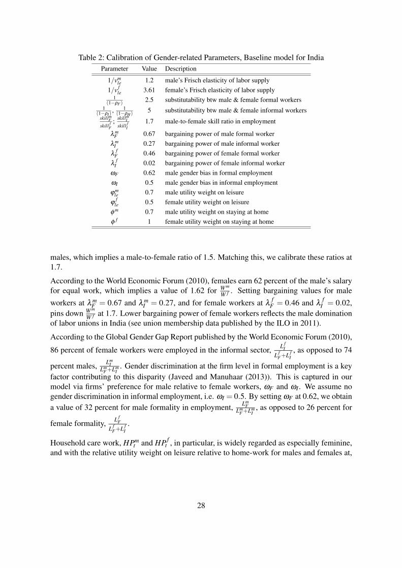
Table 2: Calibration of Gender-related Parameters, Baseline model for IndiaParameter Value Description

1/vmle 1.2 male’s Frisch elasticity of labor supply

1/v fle 3.61 female’s Frisch elasticity of labor supply

1(1−ρF )

2.5 substitutability btw male & female formal workers1

(1−ρI), 1(1−ρH ) 5 substitutability btw male & female informal workers

skillmF

skill fF

; skillmI

skill fI

1.7 male-to-female skill ratio in employment

λ mF 0.67 bargaining power of male formal worker

λ mI 0.27 bargaining power of male informal worker

λf

F 0.46 bargaining power of female formal workerλ

fI 0.02 bargaining power of female informal worker

ωF 0.62 male gender bias in formal employmentωI 0.5 male gender bias in informal employmentϕm

le 0.7 male utility weight on leisureϕ

fle 0.5 female utility weight on leisure

φ m 0.7 male utility weight on staying at homeφ f 1 female utility weight on staying at home

males, which implies a male-to-female ratio of 1.5. Matching this, we calibrate these ratios at1.7.

According to the World Economic Forum (2010), females earn 62 percent of the male’s salaryfor equal work, which implies a value of 1.62 for W m

W f . Setting bargaining values for male

workers at λ mF = 0.67 and λ m

I = 0.27, and for female workers at λf

F = 0.46 and λf

I = 0.02,pins down W m

W f at 1.7. Lower bargaining power of female workers reflects the male dominationof labor unions in India (see union membership data published by the ILO in 2011).

According to the Global Gender Gap Report published by the World Economic Forum (2010),

86 percent of female workers were employed in the informal sector, L fI

L fF+L f

I, as opposed to 74

percent males, LmI

LmF+Lm

I. Gender discrimination at the firm level in formal employment is a key

factor contributing to this disparity (Javeed and Manuhaar (2013)). This is captured in ourmodel via firms’ preference for male relative to female workers, ωF and ωI . We assume nogender discrimination in informal employment, i.e. ωI = 0.5. By setting ωF at 0.62, we obtaina value of 32 percent for male formality in employment, Lm

FLm

F+LmI

, as opposed to 26 percent for

female formality, L fF

L fF+L f

I.

Household care work, HPmt and HP f

t , in particular, is widely regarded as especially feminine,and with the relative utility weight on leisure relative to home-work for males and females at,

28

ϕmle = 0.7 and ϕ

fle = 0.5, the female to male ratio of home-work, HP f

tHPm

t, is obtained at 1.6547.

According to the NSSO report in 2009-10, female labor force participation rate, P f

p f , is 39.9

percent which is less than half of that of the male labor force participation rate, Pm

pm , at 84.8

percent. Combined with the above calibration, we obtain values of P f

p f at 39.6, and Pm

pm at81.3, by setting the male and female relative weight on utility from staying at home versusmarket-good consumption, φ m and φ f , at 0.7 and 1, respectively.

4.3. Bayesian Estimation

We estimate the model using Bayesian approach in Dynare. This choice is driven by the widelyrecognized advantages of the Bayesian-Maximum Likelihood methodology, which are as fol-lows48. First, prior information about parameters available from empirical studies or previousmacroeconomic studies, can be incorporated with the data in the estimation process. Second,it facilitates representing and taking fuller account of the uncertainties related to models andparameter values. Third, it allows for a formal comparison between different mis-specifiedmodels that are not necessarily encapsulated in the marginal likelihood of the model. In ad-dition, there has been a growing trend among central banks to employ Bayesian methods forconducting policy analysis.

Table 3 summarizes the choice of prior distributions for the estimated parameters. The priordensities for the estimated parameters are chosen by considering the theoretical restrictions forthe parameters, and empirical evidence. Due to scarce empirical evidence on India, we chooserelatively diffuse priors that cover a wide range of parameter values. The use of a diffuse priorreduces the importance of the mean of the prior distribution on the outcome of the estimation.

5. Empirical Results

Bayesian estimates for the parameters are summarized in Table 3, along with the 95 percentposterior confidence band. Looking at price adjustment costs, consistent with the estimates inGabriel et al. (2010), the estimation indicates that price re-setting is highest in the informalsector (φ ad j

I = 24.15), and lowest for the formal sector (φ ad jF = 64.54 ). This means that

the fluctuations in the formal sector are more persistent in response to shocks compared withthe informal sector. Import price rigidity, φ

ad jf∗ , has a posterior mean of 42.44, indicating

that import prices change more frequently in comparison to formal prices, but less frequentlyrelative to informal prices. Most emerging economies policy-related studies in the literature

47According to the Times User Survey conducted in 2010, female contribution towards unpaid domestic workin India is 10 times more than males. This unpaid work includes the inter-personal work for caring for otherhousehold members, and in countries like India with lack of sufficient infrastructure, the work of collectingwater and fuel for household needs.

48See, for instance, An and Schorfheide (2007).

29

do not allow the pricing parameters to differ across the tradable and non-tradable sectors. Thisputs a warning sign in interpreting the estimates of price stickiness in the literature.

Estimation results suggest a strong response of the Reserve Bank of India (RBI) to inflationdeviations in the economy (απ = 3.2) and significantly lesser to output deviations (αY = 0.32),along with considerable policy inertia (αi = 0.86). The estimates for αY and αi are in the rangeof previous studies49, whereas απ is estimated to be slightly higher than the previous valuesin the literature, that range from 1.5 to 2.9 across different studies50. This may be the result ofthe combined shock-absorbing role of the informal sector and of low skilled female workers,because of which the RBI needs to be more aggressive in order to stabilize prices.

The persistence of most of the shocks in the economy are estimated to be high ranging from0.58 to 0.97, with the exception of a few51. Posterior estimated means for the standard devia-tion of shocks are significantly higher than the corresponding prior means, which is consistentwith higher business cycle volatility associated with emerging economies.

Overall, we obtain reasonable estimates for the common parameters used in other studies, inthe sense that all of them are statistically significant and most of them are in the range ofestimates in the existing studies on emerging economies relying on Bayesian DSGE models.Some of our estimates turn out to be away from the prior means, such as for κ , φ

ad jF , φ

ad jI , φ

ad jf ∗ ,

and for ρπ , ρθF , ρθI , which suggests that the data is quite informative about these parameters.In addition, robustness checks described in Appendix A indicate that our estimation analysis isrobust to the prior specification, which confirms that our arguments are strongly supported bythe data. However, for some parameters, the data does not provide additional information52.We believe that our estimation results should be considered as preliminary estimates, andfurther work is necessary to ensure a robust identification of the key gender-related parameters.

6. Policy Results

6.1. Gender-Specific Policies

In this section, we study the dynamic impact of the following gender-specific policies: (i) in-crease in public provisions (including childcare support); (ii) improvements in female safetyand mobility; (iii) increase in female education; and (iv) stronger enforcement of laws againstemployment based gender discrimination. The former two policies lower constraints on fe-male labor supply, whereas the latter two are targeted towards lowering female labor demandconstraints.

49Gabriel et al. (2010) and Anand et al. (2010) estimate similar numbers for India.50The estimates for India range from 0.89 in Anand et al. (2010) to 2.5 in Gabriel et al. (2010). For other

developing countries, it ranges from 1.27 in Castillo et al. (2006) for Peru to 2.6 in Tovar (2006a) for Korea.51These include shocks to female worker skill in formal employment, ρskillF , male gender-bias in formal em-

ployment, ρωmF

, and the informal technology shock, ρθI , that have posterior means of 0.37, 0.10, and 0.33,respectively.

52This does not impact the results of our policy analysis.

30

To see how the economy transitions from the initial to the new steady state post-reform, weconsider a permanent shock to the relevant variables. Table 5 summarizes the short run andlong run impact of reforms on aggregate economic activity (i.e. GDP, formality in the labormarket, and unemployment), and on labor market indicators of gender inequality (female laborforce participation, female formality, and gender wage gaps).

Female Labor Supply Reforms

The impact of policies that lower constraints on female labor supply is a combination of itsdirect impact on female labor force participation, combined with its indirect impact on thesame through changes in wages and employment in each sector.

(i) Increase in Public Provisions (including childcare)

Home production consists of both childcare and other household activities, where an increasein public provisions53 lowers the burden of home-work for all individuals in the household,which is captured by an increase in the home-production technology, θH . Childcare provi-sions, on the other hand, are assumed to be targeted towards females, which is captured by asimultaneous fall in 1

ϕf

le.

Figure 3 shows the combined effect of an increase in θH and a fall in 1ϕ

fle

. An improvement

in public provisions which increases female labor participation by 1.5 percent would lead toa 1.4 percent gain in GDP. However, it would also increase aggregate unemployment andinformality by 1 and 0.1 percent, respectively, along with widening gender gaps in the same54.Below we provide a detailed analysis of the main channels at play.

Higher productivity of home production implies that males and females can consume the sameamount of home goods with lower amount of home-work. Substitution effect leads to an in-crease in male and female labor force participation in the long run. Childcare support targetedtowards females ( 1

ϕf

lefalls) leads to a larger increase in P f , thus lowering gender gap in par-

ticipation rates, P f

Pm . Increase in overall labor supply and employment raises GDP. However,owing to the presence of labor market rigidities, increase in labor supply is not met with anequal increase in firm hiring, leading to an increase in unemployment, U . In addition, informalwholesalers hire more workers relative to ones in the relatively rigid formal sector, thus alsoreducing overall formality in the labor market, LF

LF+LI.

More males relative to females get employed and are able to find formal employment, leadingto a larger fall in female formality in comparison to that for males, which further widenswage gaps; W m

W f increases. This is due to the higher constraints females face in their accessto decent formal employment, including lower skills and gender-based discrimination against

53This refers to better water facilities, sanitation development, access to electricity etc.54This is induced by a 1 percent increase in θH and a 5 percent fall in 1

ϕf

le.

31

women. At home, relative burden of females’ home-work, HP f

HPm , is now lower, improvinggender equality at home55.

Qualitatively, the short run impacts of policy are similar to the ones in the long run. However,due to relatively higher rigidities, formal wholesalers increase hiring only gradually over timewhich increases unemployment and lowers aggregate, female and male formality by more inthe short run.

Figure 3: Increase in Public Provisions (including childcare)

Note: The figure shows a percentage deviation from the initial steady state for GDP, while for the rest of thevariables the levels (%) are shown.

(ii) Increase in Female Safety and Mobility

Improvements in safety and mobility of females directly lowers females’ relative disutilityfrom working outside home, which is captured by a fall in φ f in Figure 456.

Qualitatively, the impacts on GDP and labor market indicators of gender inequality are similarto the ones with the policy of increased public provisions. However, there is an increase ingender inequality in relative burden of female-to-male home-work, as opposed to a decrease

55Increase in the relative proportion of female wage income in total household income increases their intra-household bargaining power, (1−BPt), leading to females opting out of home-work into market-work andleisure. Instead, males now substitute out of leisure into market-work and home-work.

56This is induced by a 10 percent fall in φ f .

32

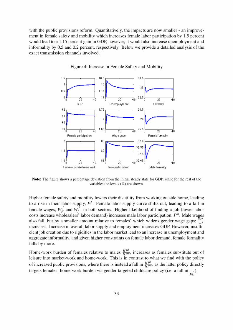
with the public provisions reform. Quantitatively, the impacts are now smaller - an improve-ment in female safety and mobility which increases female labor participation by 1.5 percentwould lead to a 1.15 percent gain in GDP, however, it would also increase unemployment andinformality by 0.5 and 0.2 percent, respectively. Below we provide a detailed analysis of theexact transmission channels involved.

Figure 4: Increase in Female Safety and Mobility

Note: The figure shows a percentage deviation from the initial steady state for GDP, while for the rest of thevariables the levels (%) are shown.

Higher female safety and mobility lowers their disutility from working outside home, leadingto a rise in their labor supply, P f . Female labor supply curve shifts out, leading to a fall infemale wages, W f

F and W fI , in both sectors. Higher likelihood of finding a job (lower labor

costs increase wholesalers’ labor demand) increases male labor participation, Pm. Male wagesalso fall, but by a smaller amount relative to females’ which widens gender wage gaps; W m

W f

increases. Increase in overall labor supply and employment increases GDP. However, insuffi-cient job creation due to rigidities in the labor market lead to an increase in unemployment andaggregate informality, and given higher constraints on female labor demand, female formalityfalls by more.

Home-work burden of females relative to males HP f

HPm , increases as females substitute out ofleisure into market-work and home-work. This is in contrast to what we find with the policyof increased public provisions, where there is instead a fall in HP f

HPm , as the latter policy directlytargets females’ home-work burden via gender-targeted childcare policy (i.e. a fall in 1

ϕf

le).

33

Female Labor Demand Reforms

The impact of policies that lower constraints on female labor demand is a combination of itsdirect impact on female employment, and its indirect impact on labor market participationrates, through changes in wages and employment creation in each sector.

(iii) Increase in Female Education

Figure 5 shows the effect of an increase in the skill level of female workers in both sectors,skill f

F and skill fI . In the long run, an increase in female education which raises female labor

participation by 1.5 percent would raise GDP by 1.25 percent, lower unemployment by 1.75percent and increase labor formality by 0.9 percent57. In addition, it lowers gender gapsin participation rate, formal employment, and wages. In the short run, however, there areadjustment costs in terms of a fall in female formality and wider gender wage gaps, whichlasts up to 4 quarters.

Figure 5: Increase in Female Worker Skill

Note: The figure shows a percentage deviation from the initial steady state for GDP, while for the rest of thevariables the levels (%) are shown.

Increase in females’ skill level improves their productivity in the labor market, leading towholesalers substituting out male workers for more productive female workers in both sectors.

57This is induced by a 5 percent increase in both skill fF and skill f

I .

34

More females are hired in the formal relative to the informal sector, thus increasing female

formality in labor employment, L fF

L fF+L f

I, in the long run. Instead, we see a fall in the short run

(up to 4 quarters), as higher flexibility of the informal labor market leads to an immediateincrease in female informal employment, as opposed to a gradual increase in female formalemployment over time. Higher job-finding rate increases females’ return from job search,which increases female labor supply, P f . The positive impact of higher productivity of femaleworkers on wages outweighs the negative impact of higher female labor supply in the longrun, leading to an increase in female wages, W f

F and W fI , in both sectors. However, female

wages are lower in the short run as the latter effect dominates given slow job creation . Maleparticipation rate declines due to two reinforcing effects - (i) household income effect: higherfemale wage incomes increase total household income, and (ii) substitution effect: fall in malejob-finding rate reduces their return from job search58. Male labor supply curve shifts inwards,leading to an increase in their wages in both sectors. Higher aggregate formality and lowerunemployment boosts GDP in the long run. At home, HP f

HPm falls as females substitute outof home-work into market-work and leisure, and males on the other hand, substitute out ofmarket-work and leisure into home-work.

(iv) Lower Gender Discrimination in Formal Employment

Figure 6 shows the effect of a decrease in formal wholesalers’ relative preference for malerelative to female workers in formal employment, ωF

59. This corresponds to stronger en-forcement of laws against gender-based discrimination in employment. Results indicate thatgender equality in the labor market and at home improve, i.e. gender gaps in labor participa-tion rates, wages, formal employment, and relative home-work burden are reduced. However,unless accompanied by higher female education, we see a fall in aggregate economic activity,i.e. GDP and formality are lower in the long run.

With this policy, formal wholesalers are forced to substitute out higher skilled male workersfor relatively lower skilled female workers, increasing female formality. This reduces overallproductivity and profits in the formal sector, which shrinks aggregate formality and worsensGDP60.

Higher probability of getting formal employment increases females’ returns to job search,which raises female labor supply, P f .61 In contrast to the female education reform whichleads to an increase in wages of both males and females in the new steady state, we find thatfemale wages are higher, but male wage rates in both sectors are now lower. This is becausedemand for female relative to male workers is higher in the formal sector, increasing W f

F while

58Fall in male informal employment is higher relative to their fall in formal employment, thus increasing overallmale formality, Lm

FLm

F+LmI

.59Since informal firms are not regulated, ωI remains unchanged.60This effect is a result of our assumption regarding homogenous male and female workers. Instead, allowing

for heterogeinity in skill level might lead to a different outcome.61Gonzalez et al. (2015) find that the presence of gender-based legal restrictions are strongly associated with

larger gender gaps in labor force participation.

35

lowering W mF . Female workers move from informal to formal jobs, reducing their supply to

informal wholesalers, which increases W fI , and vice-versa for males. Male participation, Pm,

falls due to two reinforcing income and substitution effects discussed above. Impact at homefollows analogously from the policy of increase in female skill discussed above.

Figure 6: Lower Gender Discrimination in Formal Employment

Note: The figure shows a percentage deviation from the initial steady state for GDP, while for the rest of thevariables the levels (%) are shown.

To summarize, the above results indicate the following. First, policies targeted towards re-ducing constraints on female labor supply, directly increase female labor force participation,reducing gender gaps in participation rates. However, due to labor market rigidities, thesepolicies are unable to simultaneously generate enough employment creation in the formal sec-tor, leading to an increase in aggregate informality and unemployment. In addition, givengender-specific constraints on females’ access to decent formal jobs, it also worsens gendergaps in wages and informal employment. Regarding gender dynamics at home, increase inpublic provisions by directly reducing females’ childcare burden improves gender division inhome-work and leisure, whereas it worsens with higher female safety and mobility. Second,effects of the two policies targeted towards reducing female labor demand constraints vary. In-crease in the skill level of females along with reducing gender gaps in participation rates, alsosimultaneously leads to adequate formal job creation due to increase in overall formal sectorproductivity. Aggregate formality and employment increase, resulting in higher formality inmale and female employment, while also lowering gender gaps in wages and informal em-ployment. However, female formality in employment falls in the short run. On the other hand,

36

unless accompanied by an increase in female education, strengthening firm-based discrim-ination laws forces firms to hire lower skilled female workers, thus lowering formal sectorproductivity, which shrinks formality and GDP in the economy.

Comparing our results to the ones in the gender-based policy literature, the impact on femalelabor force participation and GDP is consistent with these studies, both qualitatively and quan-titatively. However, our framework is additionally able to capture the impact on the femalequality of employment, female unemployment rate, and gender wage gaps, which even thoughshown to be empirically relevant, is largely ignored in this theoretical literature.

6.2. Labor Market Deregulation

Figure 7: Labor Market Deregulation in the Formal Sector

Note: The figure shows a percentage deviation from the initial steady state for GDP, while for the rest of thevariables the levels (%) are shown.

Figure 7 shows the combined effect of a decrease in formal wholesalers’ labor hiring cost,βHCF , and a fall in the bargaining power of male workers in the formal sector, β m

F62. In the

long run, lower labor regulations that decrease informality by 1.5 percent would increase GDPby 2 percent and lower unemployment by 1.5 percent, but due to gender related constraints

62We do not shock the bargaining power of female workers, βf

F , as we already assume a considerably smallvalue for this due to male domination in labor unions. Thus, even after a 10 percent fall in β m

F , the gendergap in bargaining power is substantially large.

37

females face in their access to decent formal employment, male workers gain more, leading towider gender gaps in formal employment. This combined with the household income effectlowers female labor participation, which falls by 0.5 percent63. In addition, in the short run,during the transition to the new steady state, unemployment increases and GDP falls, that lastsup to 4 quarters post-reform64.

There are two opposing effects on male and female participation rates, Pm and P f : (i) substi-tution effect: increase in job-finding rate in the formal sector produces higher returns to jobsearch, increasing P f and Pm, and (ii) household income effect: as more household membersare employed in higher paying formal jobs, this increases total household income, which de-creases P f and Pm. For males, substitution effect outweighs the income effect in the short run,increasing Pm, whereas it decreases in the long run due to stronger income effects. In contrast,due to a smaller increase in female’s job-finding rate in the formal sector relative to males(due to gender-related constraints, including education gaps and discrimination by firms), thehousehold income effect outweighs the substitution effect for females in both the short runand long run, decreasing P f . Therefore, gender gaps in participation rates widen; P f

Pm falls.

Increase in male labor supply, Pm, has a negative impact on their wages, whereas decrease infemale labor supply, P f , has a positive impact on female wages, thus lowering gender wagegaps. At home, a larger increase in aggregate wage income of males relative to females, leadsto a fall in the intra-household female bargaining power, worsening gender division in home-work; HP f

HPm increases.

6.3. Reform Interactions

Given the above policy outcomes, in this section, we ask the following question: what isthe optimal strategy for implementing gender-specific reforms, one that will lead to gains inaggregate economic outcomes, and simultaneously improve gender equality in labor force par-ticipation, wages, and formal employment? We study the impact of implementing a combinedpackage of reforms. Specifically, we look at three cases: (i) combining a female labor supplyreform with a female labor demand side reform, (ii) combining a female labor supply reformwith a labor market deregulation reform, and (iii) combining two female labor supply sidereforms.

Figure 8 shows the effects of a simultaneous reform package (black solid line) combining im-provements in female safety and mobility (blue dashed line) with increase in female education(red dashed line). In contrast to when only the former reform is implemented, which leads toa fall in female and aggregate formality, higher unemployment, and wider gender wage gapsin the economy, combining it with the latter reform instead overturns these adverse outcomes.It helps mitigate the short run fall in female formality associated with the education reform,

63This is induced by a 5 percent fall in βHCF and β mF .

64This is consistent with the findings in the literature on market regulations. See, for instance, Blanchard andGiavazzi (2003), Cacciatore et al. (2012), and Cacciatore et al. (2013), for details regarding the transmissionchannels involved.

38

Figure 8: Improvements in Female Safety and Skill

Note: The blue dashed line corresponds to increase in female safety and mobility, the red dashed linecorresponds to the policy of increase in female skill, and the black solid line is the policy impact with a

combination of both policies. The figure shows a percentage deviation from the initial steady state for GDP,while for the rest of the variables the levels (%) are shown.

while also leading to significantly higher gains in GDP. Better safety and mobility outsidehome increases female labor supply, P f , and due to a simultaneous increase in their skills,which increases female labor productivity, a larger proportion of these females get hired byformal relative to informal wholesalers, who also pay higher wages. Higher probability ofgetting employed and higher wages reinforces the positive impact on female participation,increasing it by more than when either policy is implemented on its own. Both substitutionand income effect lower male participation, Pm. At home, increase in female wage incomeimproves their intra-household bargaining power, thus reducing their home-work burden; HP f

HPm

falls.

Figure 9 shows the effect of a simultaneous reform package (black solid line) combiningthe policy of increase in female safety and mobility (blue dashed line) with a labor marketderegulation reform (red dashed line). We find that in contrast to when the former policy isimplemented on its own, unemployment is lower, both female and male formality increases,and gender wage gaps are lower. Moreover, female labor force participation increases, as op-posed to a decrease when labor market deregulation policy is implemented on its own. Bettersafety and mobility of females outside home, directly increases their labor participation rate,where these females are now able to find high paying formal jobs, as the formal sector expandsdue to lower formal labor market rigidities. This expansion of the formal sector also increases

39

Figure 9: Increase in Female Safety and Labor Market Deregulation

Note: The blue dashed line corresponds to increase in female safety and mobility, the red dashed linecorresponds to the formal labor market deregulation, and the black solid line is the policy impact with a

combination of both policies. The figure shows a percentage deviation from the initial steady state for GDP,while for the rest of the variables the levels (%) are shown.

male formality in employment, which leads to higher male participation, as their return fromjob search is now higher. Thus, GDP increases by more now. Moreover, it also increases in theshort run as opposed to when only the deregulation reform is implemented, however, there is alarger short run increase in unemployment65. The larger increase in unemployment is causedby two factors: increase in both male and female participation, and slower creation of jobs inthe formal relative to the informal sector.

Figure 10 shows the effect of a simultaneous reform package combining the policy of increasein female safety and mobility with increase in public provisions. Since both reforms lowerfemale labor supply constraints, there is a larger increase in female labor force participationrate, in contrast to when either policy is implemented on its own. Both policies are associatedwith inadequate formal job creation, which reinforces their individual impact resulting in aneven larger increase in informality and unemployment.

Therefore, we find that not all combined policy packages lead to higher gains. In particular,we find that there is a complementarity in the impacts of policies that lower constraints onfemale labor participation and policies that boost formal job creation, leading to gains in both

65We find that a combined package of labor market deregulation and female education reform helps overturnthis short run increase in unemployment.

40

Figure 10: Increase in Female Safety and Public Provisions

Note: The blue dashed line corresponds to increase in female safety and mobility, the red dashed linecorresponds to increase in public provisions (including childcare), and the black solid line is the policy impactwith a combination of both policies. The figure shows a percentage deviation from the initial steady state for

GDP, while for the rest of the variables the levels (%) are shown.

gender equality and overall economic activity. Based on the above findings, we suggest thatpolicies should be designed to prioritize getting females into paid work outside home (i.e.lower constraints on female labor supply), while at the same time making sure that there areenough formal job opportunities (i.e. lower labor market rigidities in the formal sector), andthat females have access to these formal jobs (i.e. lower constraints on female labor demand).

7. Conclusion

In this paper, we investigate the interaction between informality and gender inequality in the labor market. Specifically, we study the impact of a number of gender-specific policies on female labor force participation, their access to formal employment, gender wage gaps, as well as on aggregate economic outcomes. To achieve this goal, we build a small open economy DSGE model by incorporating both gender inequality and informality within our framework. The model is estimated using Bayesian techniques and applied to Indian data. Our framework integrates the literature on gender with the literature on labor market rigidities, and is detailed enough to provide a starting point for studying the impact of various public policies.

41

In our model, we have two sectors, formal and informal sector, where informality results fromsignificantly higher rigidities in the formal sector. Households consist of males and females,where gender inequality is modeled as various frictions on their labor supply and demand,which are higher for females relative to males. Using this framework, we investigate theimpact of the following gender-specific policies: (i) increase in female education; (ii) increasein public provisions (including childcare); (iii) increase in female safety and mobility to work;and (iv) fall in gender-based discrimination by firms in formal employment. In addition, theimpact of lowering labor market rigidities (i.e. labor market deregulation) in the formal sector,is also considered.

Our findings carry both good and bad news. First, on the one hand, gender-targeted policies increase female labor force participation and GDP in both the short run and long run. On the other hand, however, due to labor market rigidities, gender-specific policies do not generate sufficient formal job creation. This results in a larger share of these increased female participants either being employed informally at low wages, or staying unemployed, which increases aggregate unemployment and informality and further widens gender gaps in wages and informal employment. The only exception to this is with the policy that increases female education, which by increasing female workers’ efficiency at work, leads to higher formal employment of females. In addition, this increase in female efficiency leads to an expansion of the formal sector engendering an increase in both female and male formal employment. However, slow reallocation of workers due to labor market rigidities leads to a fall in female formality and widens gender wage gaps in the short run.

Second, there is an increase in the formal employment of both males and females with a labor market deregulation reform. However, male workers gain more, as constraints on female labor supply and demand combined with the household income effect lowers female participation and lead to a smaller increase in female formality in comparison to males. Finally, we show that simultaneously implementing gender-based policies that lower constraints on female par-ticipation combined with policies that boost formal job creation, as opposed to a piecemeal approach, generates substantial gains in gender equality in participation, formal employment, and wages along with larger gains in GDP and formality.

42

References

[1] Acemoglu, D., Autor, D. H. and Lyle, D.S. (2004). Women, War, and Wages: The Effectof Female Labor Supply on the Wage Structure at Mid-Century. Journal of PoliticalEconomy, 112 (3), 497–551, June 2004.

[2] Agenor, P.R. (2012). A Computable OLG model for Gender and Growth Policy Analysis.Mimeo, University of Manchester and World Bank.

[3] Agenor P.R. and Canuto, O. (2013). Gender Equality and Economic Growth in Brazil: aLong-Run Analysis. Policy Research Working Paper, No. 6348, World Bank, January.

[4] Agenor, P.R. (2015). Gender Equality and Economic Growth: An Overlapping Genera-tions Model for India. OECD Working Paper. Forthcoming.

[5] Aguiar, M. and Gopinath, G. (2007). Emerging Market Business Cycles: The cycle isthe trend. Journal of Political Economy, 115, 69–112.

[6] Albanesi, S. and Patterson, C. (2014). Explaining the Behaviour of Aggregate Hours inthe US: The Role of Gender. Mimoe, Federal Reserve Bank of New York.

[7] Anand, R., S. Peiris, and M. Saxegaard (2010). An Estimated Model with MacrofinancialLinkages for India. IMF Working Paper, WP/10/21, International Monetary Fund.

[8] An, S. and Schorfheide, F. (2007). Bayesian Analysis of DSGE Models. EconometricsReviews, Volume 26 (2-4), 113-172.

[9] Barro, R.J. and Lee, J.W. (2013). A New Data Set of Educational Attainment in theWorld, 1950-2010. Journal of Development Economics, 104, 184-198.

[10] Becker, G.S. (1965). A Theory of the Allocation of Time. The Economic Journal, Vol.75 (299), pp. 493–517.

[11] Besley, T. and Burgess, R. (2004). Can Labor Regulation Hinder Economic Perfor-mance? Evidence from India. The Quarterly Journal of Economics, 119: 91-134.

[12] Blanchard, O. and Gali, J. (2006). A New Keynesian Model with Unemployment. Na-tional Bank of Belgium Working Paper, No. 92, October 2006.

[13] Blundell, R. and MaCurdy, T. (1999). Labour Supply: A Review of Alternative Ap-proaches. Handbook of Labor Economics Vol. 3A, 1999, 1560-1695.

[14] Campbell, D. and Ahmed, I. (2012). The Labour Market in Developing Countries,” IZA,September 19.

[15] Campolmi, A. and Gnochhi, S. (2014). Labor Market Participation, Unemployment, andMonetary Policy. Bank of Canada Working Paper, European Central Bank.

[16] Castillo, P., Montoro, C. and Teusta, V. (2006). An Estimated Stochastic General Equi-librium Model with Partial Dollarization: A Bayesian Approach. Central Bank of ChileWorking Papers, 381.

[17] Castillo, P. and Montoro, C. (2008). Monetary Policy in the Presence of Informal LabourMarkets. Mimeo, Banco Central de Reseva del Peru.

43

[18] Cavalcanti, T.V.D.V. and Tavares, J. (2008). The Output Cost of Gender Discrimina-tion: A Model-Based Macroeconomic Estimate. Proceedings of the German Develop-ment Economics Conference, Zürich 2008 (No. 43).

[19] Chandrasekhar, C.P. and Ghosh, J. (2015). Growth, employment patterns and inequalityin Asia: A case study of India. ILO Asia-Pacific Working Paper Series, InternationalLabour Organization (ILO), January 2015.

[20] Christiano, L.J, Eichenbaum, M.S. and Trabandt, M. (2014). Understanding the GreatRecession. NBER Working Paper, 20040.

[21] Conesa, J.C., Diaz-Moreno, C. and Galdon-Sanchez, J.E. (2002). Explaining Cross-Country Differences in Participation Rates and Aggregate Fluctuations. Journal of Eco-nomic Dynamics and Control, 26, 333-345.

[22] Cuberes, D. and Teigner, M. (2014). Gender inequality and Economic Growth: A CriticalReview. Journal of International Development, Vol. 26, Issue 2, pp. 260-276, March2014.

[23] Das, S., Jain-Chandra, S., Kochhar, K. and Kumar, N. (2015). Women Workers in India:Why So Few Among So Many? IMF Working Paper, 15/55, Washington, InternationalMonetary Fund.

[24] Dixit, A.K. and Stiglitz, J. (1977). Monopolistic Competition and Optimum ProductDiversity. The American Economic Review, 67, 297-308.

[25] Dollar, D. and Gatti, R. (1999). Gender Inequality, Income, and Growth: Are GoodTimes Good for Women? Policy Research Report on Gender and Development WorkingPaper Series, No. 1, May 1999.

[26] Duflo, E. (2012). Women Empowerment and Economic Development. Journal of Eco-nomic Literature, Vol. 50, No. 4: pp. 1051-079.

[27] Elborgh-Woytek, K., Newiak, M., Kochhar K., Fabrizio, S., Kpodar, K., Wigender P.,Clements B., and Schwartz, G. (2013). Women, Work, and the Economy: Macroeco-nomic Gains from Gender Equity. IMF Staff Discussion Note 13/10, Washington, Inter-national Monetary Fund.

[28] Esteve-Volart, B. (2009). Gender discrimination and growth: Theory and evidence fromIndia. Mimeo.

[29] Mendoza, E.G. (1991). Real Business Cycles in a Small Open Economy. The AmericanEconomic Review, Vol. 81, No. 4 (Sep., 1991), 797-818.

[30] Fontana, M. and Wood, A. (2000). Modeling the Effects of Trade on Women, at Workand at Home. World Development, Vol 28 No 7.

[31] Fontana, M. (2004). Modelling the effects of trade on women, at work and at home:Comparative Perspectives. Economic Internationale, 99, 49-80.

[32] Gabriel, V.J., Levine, P., Pearlman, J. and Yang, B. (2010). An Estimated DSGE Modelof the Indian Economy. Discussion Paper in Economics, DP 12/10, University of Surrey.

44

[33] Galor, O. and Weil, D. N. (1996). The gender gap, fertility, and growth. American Eco-nomic Review, 85(3), 374–387.

[34] Gonzalez, C., Jain-Chandra, S., Kochhar K. and Newiak M. (2015). Fair Play: MoreEqual Laws Boost Female Labor Force Participation. IMF Staff Discussion Note 15/02,Washington, International Monetary Fund.

[35] Hendy, R. and Zaki, C. (2010). Assessing the Effects of Trade Liberalization on WageInequalities in Egypt: A Microsimulation Analysis, ERF Working Paper, 555.

[36] Hsieh C.T., Hurst, E., Jones, C.I. and Klenow, P.J. (2013). The allocation of talent andU.S. economic growth. NBER Working Paper, No. 18693, January 2013.

[37] ILO (2011). Trade Union Membership Statistics. ILO Department of Statistics.

[38] ILO (2012). Statistical Update on Employment in the Informal Economy. InternationalLabour Organization, Department of Statistics. June 2012.

[39] Javeed, S. and Manuhaar, A. (2013). Women and Wage Discrimination in India: A Crit-ical Analysis. International Journal of Humanities and Social Science Invention, Vol. 2,Issue 4, April 2013, pp. 06-12.

[40] Klasen, S. (1999). Does Gender Inequality Reduce Growth and Development? Evidencefrom Cross-Country Regressions. Policy Research Report on Gender and DevelopmentWorking Paper Series, No. 7, November 1999.

[41] Klasen, S. and Lamanna, F. (2009). The Impact of Gender Inequality in Education andEmployment on Economic Growth: New evidence for a panel of countries. FeministEconomics, 15(3), 91-132.

[42] Klasen, S. and Pieters, J. (2015). What Explains the Stagnation of Female Labor ForceParticipation in Urban India. World Bank Economic Review, Vol. 29, pp. 1-30.

[43] Medina, J.P. and Soto, C. (2005). Oil Shocks and Monetary Policy in an Estimated DSGEModel for a Small Open Economy. Mimeo, Central Bank of Chile.

[44] Mitra, A. and Verick, S. (2013). Youth Employment and Unemployment: An IndianPerspective. ILO Asia Working Paper Series, ISSN 2227-4491, International Labour Or-ganization (ILO).

[45] NCEUS (2009). Report on Definitional and Statistical Issues Related to the InformalEconomy. National Commission for Enterprises in the Unorganized Sector (NCEUS),New Delhi.

[46] OECD (2008). The Price of Prejudice: Labour Market Discrimination on the Groundsof Gender and Ethnicity. Organization for Economic Cooperation and Development(OECD).

[47] Pal, R. and Rathore, U. (2013). Estimating Workers’ Bargaining Power and Firms’Markup in India: Implications of Reforms and Labour Regulation, Indira Gandhi In-stitute of Development Research, IGIDR Working Paper, WP-2014-037.

[48] Rotemberg, J. (1982). Sticky prices in the Unites States. Journal of Political Economy,Vol. 90, No. 6, Dec. 1982, pp. 1187-1211.

45

[49] Sahoo, A. and Raa, T.T. (2009). The Relative Performance of Formal and Informal Sec-tors in India. Economic Systems Research, 21:2, 151-162.

[50] Satchi, M. and Temple, J. (2009). Labor Markets and Productivity in Developing Coun-tries. Review of Economic Dynamics, 26, 333-345.

[51] Sharma, S. (2009). Entry Regulation, Labor Laws, and Informality. Working Paper, En-terprises Analysis Unit, The World Bank.

[52] Sinha, P. (2013). Combating Youth Unemployment in India. Mimeo, Berlin, Friedrich-Ebert-Stiftung.

[53] Tobin, J. (1969). A General Equilibrium Approach to Monetary Theory. Journal ofMoney, Credit and Banking, 1(1): 15-29.

[54] Tovar, C. (2006a). Devaluations, Output, and the Balance Sheet Effect: A StructuralEconometric Analysis. BIS Working Papers, No 215, September 2006.

[55] Ulyssea, G. (2009). Regulation of entry, labor market institutions and the informal sector.Journal of Development Economics, 91 (2010) 87-99.

[56] World Bank (2011). World Development Report 2012. Gender Equality and Develop-ment, The World Bank Group, Washington.

[57] World Bank (2013a). World Development Indicators, 2013.http://data.worldbank.org/data-catalog/worlddevelopment-indicators. The WorldBank Group, Washington.

[58] World Economic Forum (2010). The Global Gender Gap Report 2010. Basel, WorldEconomic Forum (WEF).

[59] World Economic Forum (2014). The Global Competitiveness Report 2014-15, Full DataEdition. Basel, World Economic Forum (WEF).

[60] World Economic Forum (2014a). The Global Gender Gap Report 2014. Basel, WorldEconomic Forum (WEF).

[61] Zenou, Y. (2008). Job Search and Mobility in Developing Countries: Theory and PolicyImplications. Journal of Development Economics, 86, 336-355.

46

A. Appendix: Estimation Results

Table 3: Prior and Posterior Distributions, Baseline Model (India)Parameter Description Dist. Prior Posterior

Mean Std. Dev. Mean 95% CB

hC Habit B 0.6 0.25 0.3993 [0.3406, 0.4523]φ

ad jF Price A.C. in F G 50 20 64.546 [60.710, 68.270]

φad jI Price A.C. in I G 50 20 24.1511 [20.240, 27.860]

φad jf ∗ Price A.C. in f* G 20 20 42.4417 [38.750, 45.610]

κ Cap. A.C. IG 20 20 6.3579 [5.0900, 7.3700]χ Country premium IG 0.002 0.002 0.0009 [0.0007, 0.0010]αi Coef. of it−1 B 0.75 0.20 0.862 [0.8249, 0.9000]απ Coef. of π G 3 3 3.2349 [2.8987, 3.5581]αY Coef. of GDP G 0.4 0.2 0.3246 [0.2821, 0.3675]ρθF Pers. of θF B 0.75 0.20 0.9718 [0.9579, 0.9883 ]ρθ I Pers. of θI B 0.65 0.20 0.3301 [0.2731, 0.4147]ρG Pers.of G B 0.75 0.20 0.7886 [0.7050, 0.8782]ρθH Pers. of θH B 0.65 0.20 0.6989 [0.6493, 0.7559]ρβHCF Pers. of βHCF B 0.75 0.20 0.778 [0.6911 0.8604 ]ρλ m Pers. of λ m

F B 0.75 0.20 0.5823 [0.5387, 0.6232]ρskillF Pers. of skill f

F B 0.75 0.20 0.3745 [0.2661, 0.4862 ]ρskillI Pers. of skill f

I B 0.75 0.20 0.772 [0.7191, 0.8310]ρφ f Pers. of φ f B 0.75 0.20 0.7348 [0.6879, 0.7835]ρϕle Pers. of ϕ

fle B 0.75 0.20 0.7782 [0.6618, 0.8775]

ρωmF

Pers. of wmF B 0.75 0.20 0.1056 [0.0671, 0.1544]

ρπ∗ Pers. of π∗ B 0.75 0.20 0.6385 [0.5942, 0.6725]ρi∗ Pers. of i∗ B 0.75 0.20 0.9492 [0.9232, 0.9751]sd(εθF) Std. Dev. of θD IG 0.01 Inf 0.1271 [0.1061, 0.1495]sd(εθ I) Std. Dev. of θI IG 0.01 Inf 0.0307 [0.0253, 0.0356]sd(εG) Std. Dev. of G IG 0.01 Inf 0.1265 [0.1016, 0.1517]sd(εθH) Std. Dev. of θH IG 0.01 Inf 0.0085 [0.0022, 0.0158]sd(εHCF) Std. Dev. of βHCF IG 0.01 Inf 0.0103 [0.0023, 0.0208]sd(ελ m) Std. Dev. of λ m

F IG 0.01 Inf 0.1121 [0.0933, 0.1316]sd(εskillF) Std. Dev. of skill f

F IG 0.01 Inf 0.0072 [0.0024, 0.0126]sd(εskillI) Std. Dev. of skill f

I IG 0.01 Inf 1.1785 [0.9458, 1.4203]sd(εφ f ) Std. Dev. of φ f IG 0.01 Inf 0.0093 [0.0023, 0.0169]sd(εϕle) Std. Dev. of ϕ

fle IG 0.01 Inf 0.009 [0.0022, 0.0166]

sd(εωF) Std. Dev. of wmF IG 0.01 Inf 0.211 [0.1622, 0.2645]

sd(επ∗) Std. Dev. of π∗ IG 0.01 Inf 0.02 [0.0024, 0.0208]sd(εi∗) Std. Dev. of i∗ IG 0.01 Inf 0.015 [0.0023, 0.0209]sd(εi) Std. Dev. of i IG 0.01 Inf 0.0084 [0.0074, 0.0096]

48

Robustness of the Result

Alternative model

We evaluate the robustness of our estimation result by re-estimating the Baseline model withalternative and less informative priors. In the alternative model, the uniform distribution is as-signed to the parameters bounded between 0 and 1, such as hC, αi, ρθH , ρskillI , ρ

ϕf

le, ρωm

F, ρφ f ,

ρβHCF, ρλ m , ρθF , ρθI , ρG, ρi∗ , and ρπ∗ , instead of beta distributions in the Baseline model66.

In addition, uniform distributions are also assigned to the monetary policy coefficient on in-flation, απ , which is bounded between 0 and 3. Table 4 compares the priors and the posteriorestimates in the alternative model with the Baseline scenario.

First of all, even though the posterior means of the Taylor rule coefficients αi , απ , and αYare smaller in the alternative model, our argument that there is considerable policy inertia, andthat the RBI responds aggressively to inflation deviations and not much to output deviations,is robust to the change in priors. Second, and our argument that formal price rigidity is higherthan informal price rigidity, and that import price rigidity falls within the range of formal andinformal price rigidity, still holds. Third, the persistence and volatility of shock processes isestimated to take high values, and thus our third argument that shocks are more persistent andvolatile in emerging economies could be maintained even under the looser prior.

Overall, even though there are some quantitative differences for estimates of some parametersin the two model specifications, Bayesian estimates are similar across the models. Thus,our estimation analysis is robust to the prior specification and our arguments are stronglysupported by the data.

66Note that the mean value of these parameters is constrained to 0.5.

49

Table 4: Robustness of Result, Alternative and Baseline Model (India)Param. Alternative Model Baseline Model

Prior Posterior Prior PosteriorDist. Mean Mean 95% C.I. Dist. Mean Mean

hC U 0.5 0.04 [0.02,0.07] B 0.6 0.3993φ

ad jF G 50 64.6 [61.52,67.43] G 50 64.546

φad jI G 50 12.95 [7.08,19.62] G 50 24.1511

φad jf ∗ G 20 40.49 [35.33,43.32] G 20 42.4417

κ IG 20 3.86 [3.40,4.32] IG 20 6.3579χ IG 0.002 0.001 [0.0008,0.0012] IG 0.002 0.0009αi U 0.5 0.79 [0.74, 0.84] B 0.75 0.862απ U 1.5 2.84 [2.62,3.00] G 3 3.2349αY G 0.4 0.05 [0.02,0.09] G 0.4 0.3246ρθF U 0.5 0.97 [0.95,0.99] B 0.75 0.9718ρθ I U 0.5 0.14 [0.09,0.18] B 0.65 0.3301ρG U 0.5 0.55 [0.48,0.60] B 0.75 0.7886ρθH U 0.5 0.76 [0.73,0.79] B 0.65 0.6989ρβHCF U 0.5 0.8 [0.62:0.69] B 0.75 0.778ρλ m U 0.5 0.79 [0.32,0.49] B 0.75 0.5823ρskillF U 0.5 0.41 [0.74,0.85] B 0.75 0.3745ρskillI U 0.5 0.80 [0.43,0.59] B 0.75 0.772ρφ f U 0.5 0.85 [0.81,0.90] B 0.75 0.7348ρϕle U 0.5 0.46 [0.40,0.55] B 0.75 0.7782ρωm

FU 0.5 0.02 [0.01,0.04] B 0.75 0.1056

ρπ∗ U 0.5 0.61 [0.56,0.72] B 0.75 0.6385ρi∗ U 0.5 0.92 [0.90,0.94] B 0.75 0.9492sd(εθF) IG 0.01 0.30 [0.25,0.35] IG 0.01 0.1271sd(εθ I) IG 0.01 0.13 [0.11,0.16] IG 0.01 0.0307sd(εG) IG 0.01 0.77 [0.63,0.94] IG 0.01 0.1265sd(εθH) IG 0.01 0.017 [0.002,0.022] IG 0.01 0.0085sd(εHCF) IG 0.01 3.64 [3.23,4.23] IG 0.01 0.0103sd(ελ m) IG 0.01 0.07 [0.05,0.09] IG 0.01 0.1121sd(εskillF) IG 0.01 0.62 [0.50,0.75] IG 0.01 0.0072sd(εskillI) IG 0.01 1.02 [0.83,1.20] IG 0.01 1.1785sd(εφ f ) IG 0.01 0.012 [0.002,0.038] IG 0.01 0.0093sd(εϕle) IG 0.01 0.015 [0.002,0.024] IG 0.01 0.009sd(εωF) IG 0.01 0.23 [0.18,0.27] IG 0.01 0.211sd(επ∗) IG 0.01 0.02 [0.015,0.023] IG 0.01 0.02sd(εi∗) IG 0.01 5.85 [5.26,6.33] IG 0.01 0.015sd(εi) IG 0.01 0.018 [0.014,0.021] IG 0.01 0.0084

50

B. Technical Appendix

This Appendix discusses the derivation of the model’s optimality conditions.

Households

Partial Derivatives of Home Production

Here we derive the partial derivatives of home-good production with respect to male andfemale home-workers, HPm

t and HP ft , and with respect to male and female leisure, lem

t andle f

t . We assume the following functional form of the home production function (Eq. 3.45):

H0t = θH,t

{[(1−BPt)(HPm

t + τUUmt )pH +(BPt)(HP f

t + τUU ft )

pH]1/pH

}1−αH

In the equation above, the total number of females unemployed can be written as: U ft =

p f −HP ft − le f

t −L fF,t −L f

I,t . Similary, for males we get Umt = pm−HPm

t − lemt −Lm

F,t −LmI,t .

Then, differencing the above with respect to HP ft :

∂H0t

∂HP ft=

(1−αH)θH,t(BPt) [1+ τU ]H0t

[HP f

t + τUU ft

]pH−1

(1−BPt)(HPmt + τUUm

t )pH +(BPt)(HP ft + τUU f

t )pH

(B.1)

and differencing the above with respect to HPmt :

∂H0t

∂HPmt

=(1−αH)θH,t(1−BPt) [1+ τU ]H0

t [HPmt + τUUm

t ] pH−1

(1−BPt)(HPmt + τUUm

t )pH +(BPt)(HP ft + τUU f

t )pH

(B.2)

Partial derivatives with respect to female leisure consumption, le ft is obtained as follows:

∂H0t

∂ le ft=−

(1−αH)θH,t(BPt) [τU ]H0t

[HP f

t + τUU ft

]pH−1

(1−BPt)(HPmt + τUUm

t )pH +(BPt)(HP ft + τUU f

t )pH

(B.3)

and similarly for males:

∂H0t

∂ lemt=−

[(1−αH)θH,t(1−BPt) [τU ]H0

t [HPmt + τUUm

t ] pH−1

(1−BPt)(HPmt + τUUm

t )pH +(BPt)(HP ft + τUU f

t )pH

](B.4)

51

Tabl

e5:

Impa

ctof

Gen

der-

Spec

ific

and

Lab

orM

arke

tRef

orm

sSh

ock

Out

put

Form

ality

Une

mp.

Fem

ale

LFP

Fem

ale

Form

alW

age

gap

YL F

/(L F

+L I)

U/

PP

f /p

fL

f F/(

Lf F+

Lf I)

Wm/W

f

Incr

ease

inpu

blic

prov

isio

nsSR

1-0

.31

2-0

.51.

04L

R1.

45-0

.11

1.5

-0.1

0.7

Incr

ease

infe

mal

esa

fety

&m

obili

tySR

0.62

-0.2

51.

281.

96-0

.48

1.07

LR

1.35

-0.1

80.

511.

5-0

.10.

70In

crea

sein

fem

ale

educ

atio

nSR

0.8

0.1

-1.3

2.4

-1.1

0.5

LR

0.7

0.15

-1.4

1.5

0.25

-0.4

Low

erfir

m-b

ased

gend

erdi

scri

min

atio

nSR

-5.7

-2-1

.53.

16

-34

LR

-8.3

-1.5

-1.3

1.5

17.5

-39.

5

Lab

orm

arke

tder

egul

atio

nSR

-0.4

50.

40.

30.

20.

5-3

LR

21.

5-1

.4-0

.52.

2-3

.5N

ote:

SRde

note

ssh

ortr

unim

pact

(with

infir

st20

quar

ters

)and

LR

deno

tes

long

run

(100

quar

ters

)im

pact

ofpo

licy.

All

valu

esar

epe

rcen

tage

devi

atio

nsfr

omst

eady

stat

e.

52

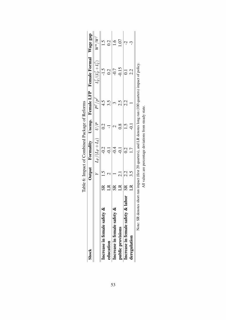
Tabl

e6:

Impa

ctof

Com

bine

dPa

ckag

eof

Ref

orm

sSh

ock

Out

put

Form

ality

Une

mp.

Fem

ale

LFP

Fem

ale

Form

alW

age

gap

YL F

/(L

F+

L I)

U/P

Pf /

pf

Lf F/(L

f F+

Lf I)

Wm/W

f

Incr

ease

infe

mal

esa

fety

&ed

ucat

ion

SR1.

5-0

.20.

24.

5-1

.51.

5L

R2

-0.1

-13.

50.

20.

2In

crea

sein

fem

ale

safe

ty&

publ

icpr

ovis

ions

SR1

-0.4

23

-0.7

1.6

LR

2.1

-0.1

0.8

2.5

-0.1

51.

07In

crea

sein

fem

ale

safe

ty&

labo

rde

regu

latio

nSR

2.2

0.2

1.5

2.2

0.1

-2L

R3.

51.

7-0

.11

2.2

-3N

ote:

SRde

note

ssh

ortr

unim

pact

(firs

t20

quar

ters

),an

dL

Rde

note

slo

ngru

n(1

00qu

arte

rs)i

mpa

ctof

polic

y.A

llva

lues

are

perc

enta

gede

viat

ions

from

stea

dyst

ate.

53

Partial Derivatives and Marginal Rate of Substitution (MRS)

Here we obtain expressions for the partial derivatives of the household utility with respectto Ct , HPm

t , HP ft , lem

t , and le ft which are then used to obtain the MRS of consumption with

respect to home production, MRShHPt ,Ct

, and with respect to leisure, MRShlet ,Ct

.

Aggregate household utility is given by Eq. 3.42 in the text as:

Λt = Et

∞

∑t=0

βt[(BPt)(pm)Λm

t +(1−BPt)(p f )Λft

]

Inserting for utility of males and females, Λmt and Λ

ft , given by Eq. 3.43 and Eq. 3.44:

Λt = E0

∞

∑t=0

βt

[(BPt)(pm)+(1−BPt)(p f )

][(1−hc)ln(Ct−hcCt−1)]

+(BPt)(pm)

[φ m

t

((H0

t )1+vm

H,t

1+νmH,t

+ϕmle,t

(lemt )

1+vmle,t

1+νmle,t

)]+(1−BPt)(p f )

[φ

ft

((H0

t )1+v f

H,t

1+νf

H,t+ϕ

fle,t

(le ft )

1+v fle,t

1+νf

le,t

)]

Partial derivative of aggregate utility with respect to Ct is the marginal utility of householdmarket-good consumption67:

∂Λt

∂Ct=

[(BPt)(pm)+(1−BPt)(p f )

](1−hc)

Ct−hcCt−1=

12

(1−hc)

Ct−hcCt−1(B.5)

Partial derivative with respect to female home production participation, HP ft yields Eq. 3.46

in the main text with h = f as:

∂Λt

∂HP ft= (BPt)(pm)

∂Λmt

∂H0t

∂H0t

∂HP ft+(1−BPt)(p f )

∂Λft

∂H0t

∂H0t

∂HP ft

We have derived ∂H0t

∂HP ft

above in Eq. B.1, and the partial derivative of female utility with

respect to home production is given by: ∂Λft

∂H0t= φ

ft

((H0

t )v f

H,t

). Similarly, for males it is:

∂Λmt

∂H0t= φ m

t

((H0

t )vm

H,t

). By inserting these in the above expression, we obtain the following:

∂Λt

∂HP ft=

[(BPt)(pm)φ m

t

((H0

t )vm

H,t

)+(1−BPt)(p f )φ

ft

((H0

t )v f

H,t

)].[

(1−αH)θH,t(BPt)[1+τU ]H0t

[HP f

t +τUU ft

]pH

(1−BPt)(HPmt +τUUm

t )pH+(BPt)(HP ft +τUU f

t )pH

] (B.6)

67We assume pm = pm = 12 and from BPt ε (0,1), we get

[(BPt)(pm)+(1−BPt)(p f )

]= 0.5.

54

Analogously, we obtain the partial derivative with respect to male home production labor:

∂Λt

∂HPmt

=

[(BPt)(pm)φ m

t

((H0

t )vm

H,t

)+(1−BPt)(p f )φ

ft

((H0

t )v f

H,t

)].[

(1−αH)θH,t(1−BPt)[1+τU ]H0t [HPm

t +τUUmt ]pH

(1−BPt)(HPmt +τUUm

t )pH+(BPt)(HP ft +τUU f

t )pH

] (B.7)

Partial derivatives with respect to female home production participation, le ft , yields Eq. 3.47

in the main text with h = f as:

∂Λt

∂ le ft= (BPt)(pm)

∂Λmt

∂H0t

∂H0t

∂ le ft+(1−BPt)(p f )

(∂Λ

ft

∂ le ft+

∂Λft

∂H0t

∂H0t

∂ le ft

)

By inserting the expressions for ∂H0t

∂ le ft

derived above in Eq. B.3, the partial derivative of female

utility with respect to home production as ∂Λft

∂ le ft= φ

ft

(ϕ

fle,t(le

ft )

v fle,t

), and for males as ∂Λm

t∂ lem

t=

φ mt

(ϕm

le,t(lemt )

vmle,t

), we obtain the following:

∂Λt

∂ le ft=

[(BPt)(pm)φ m

t

(ϕm

le,t(lemt )

vmle,t

)+(1−BPt)(p f )φ

ft

(ϕ

fle,t(le

ft )

v fle,t

)].[

(1−αH)θH,t(BPt)[−τU ]H0t

[HP f

t +τUU ft

]pH−1

(1−BPt)(HPmt +τUUm

t )pH+(BPt)(HP ft +τUU f

t )pH

] (B.8)

Similarly, we obtain the partial derivative with respect to male leisure consumption:

∂Λt

∂ lemt=

[(BPt)(pm)φ m

t

(ϕm

le,t(lemt )

vmle,t

)+(1−BPt)(p f )φ

ft

(ϕ

fle,t(le

ft )

v fle,t

)].[

(1−αH)θH,t(1−BPt)[−τU ]H0t [HPm

t +τUUmt ]pH−1

(1−BPt)(HPmt +τUUm

t )pH+(BPt)(HP ft +τUU f

t )pH

] (B.9)

The MRS between market-good and home-good consumption for females is given as:

MRS fHPt ,Ct

=

(∂Λt

∂HP ft

)/

(∂Λt

∂Ct

)

where ∂Λt

∂HP ft

is derived in Eq. B.6 and ∂Λt∂Ct

is derived in Eq. B.5. Similarly for males we get:

MRSmHPt ,Ct

=

(∂Λt

∂HPmt

)/

(∂Λt

∂Ct

)

where ∂Λt∂HPm

tis given by Eq. B.7.

55

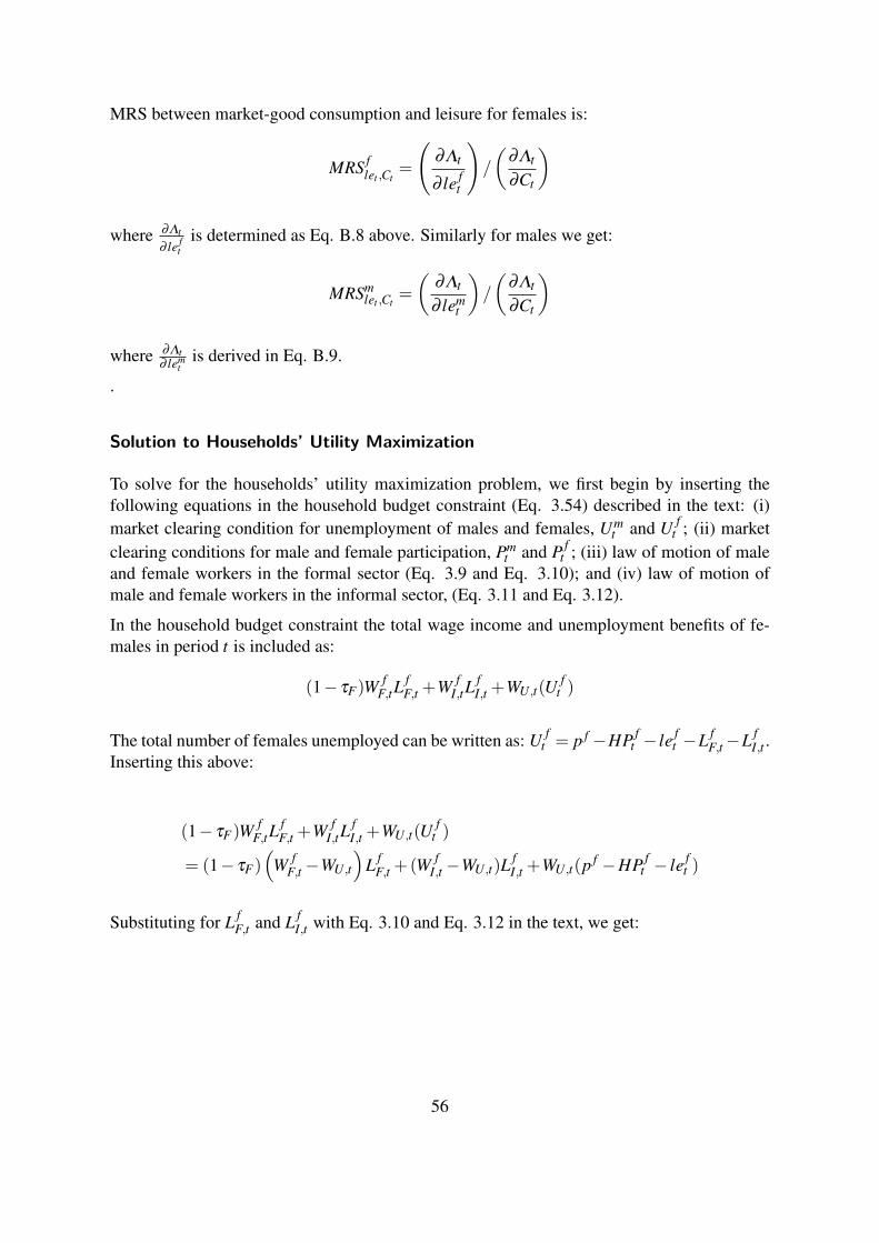
MRS between market-good consumption and leisure for females is:

MRS flet ,Ct

=

(∂Λt

∂ le ft

)/

(∂Λt

∂Ct

)

where ∂Λt

∂ le ft

is determined as Eq. B.8 above. Similarly for males we get:

MRSmlet ,Ct

=

(∂Λt

∂ lemt

)/

(∂Λt

∂Ct

)

where ∂Λt∂ lem

tis derived in Eq. B.9.

.

Solution to Households’ Utility Maximization

To solve for the households’ utility maximization problem, we first begin by inserting thefollowing equations in the household budget constraint (Eq. 3.54) described in the text: (i)market clearing condition for unemployment of males and females, Um

t and U ft ; (ii) market

clearing conditions for male and female participation, Pmt and P f

t ; (iii) law of motion of maleand female workers in the formal sector (Eq. 3.9 and Eq. 3.10); and (iv) law of motion ofmale and female workers in the informal sector, (Eq. 3.11 and Eq. 3.12).

In the household budget constraint the total wage income and unemployment benefits of fe-males in period t is included as:

(1− τF)Wf

F,tLfF,t +W f

I,tLfI,t +WU,t(U

ft )

The total number of females unemployed can be written as: U ft = p f −HP f

t − le ft −L f

F,t−L fI,t .

Inserting this above:

(1− τF)Wf

F,tLfF,t +W f

I,tLfI,t +WU,t(U

ft )

= (1− τF)(

W fF,t−WU,t

)L f

F,t +(W fI,t−WU,t)L

fI,t +WU,t(p f −HP f

t − le ft )

Substituting for L fF,t and L f

I,t with Eq. 3.10 and Eq. 3.12 in the text, we get:

56

(1− τF)Wf

F,tLfF,t +W f

I,tLfI,t +WU,t(U

ft )

= (1− τF)(

W fF,t−WU,t

)[(1−σF)(1− p(H f

F,t))LfF,t−1

]+(1− τF)

(W f

F,t−WU,t

)[p(H f

F,t)Pf

t − p(H fF,t)(1−σI)L

fI,t−1

]+(W f

I,t−WU,t)[(1−σI)(1− p(H f

I,t))LfI,t−1

]+(W f

I,t−WU,t)[

p(H fI,t)P

ft − p(H f

I,t)(1−σF)LfF,t−1

]+WU,t(p f −HP f

t − le ft )

Female labor force participation, P ft , is given by P f

t = p f −HP ft − le f

t , which when substitutedabove yields the following:

(1− τF)Wf

F,tLfF,t +W f

I,tLfI,t +WU,t(U

ft ) (B.10)

= (1− τF)(

W fF,t−WU,t

)[(1−σF)(1− p(H f

F,t))LfF,t−1

]+(1− τF)

(W f

F,t−WU,t

)p(H f

F,t)[

p f −HP ft − le f

t − (1−σI)LfI,t−1

]+(W f

I,t−WU,t)[(1−σI)(1− p(H f

I,t))LfI,t−1

]+(W f

I,t−WU,t)[

p(H fI,t)(

p f −HP ft − le f

t − (1−σF)LfF,t−1

)]+WU,t(p f −HP f

t − le ft )

Analogously, total wage income plus the unemployment benefits of males in the budget con-straint is included as:

(1− τF)W mF,tL

mF,t +W m

I,tLmI,t +WU,t(Um

t )

which can then be written as:

(1− τF)W mF,tL

mF,t +W m

I,tLmI,t +WU,t(Um

t ) (B.11)

= (1− τF)(W m

F,t−WU,t)[(1−σF)(1− p(Hm

F,t))LmF,t−1

]+(1− τF)

(W m

F,t−WU,t)[(p(Hm

F,t)(

pm−HPmt − lem

t − (1−σI)LmI,t−1

)]+(W m

I,t−WU,t)[(1−σI)(1− p(Hm

I,t))LmI,t−1

]+(W m

I,t−WU,t)[p(Hm

I,t)(

pm−HPmt − lem

t − (1−σF)LmF,t−1

)]+WU,t [pm−HPm

t − lemt ]

57

To solve the households’ utility maximization problem described in the text, we insert Eq.B.10 and Eq. B.11 derived above in the household budget constraint, and establish the associ-ated Lagrangian (L ) as follows:

E0

∞

∑t=0

βt

[(BPt)(pm)+(1−BPt)(p f )

][(1−hc)ln(Ct−hcC̃t−1)

]+(BPt)(pm)

[φ m

t

((HO

t )1+vm

H,t

1+νmH,t

+ϕmle,t

(lemt )

1+vmle,t

1+νmle,t

)]+(1−BPt)(p f )

[φ

ft

((H0

t )1+v f

H,t

1+νf

H,t+ϕ

fle,t

(le ft )

1+v fle,t

1+νf

le,t

)]

−λt

Ct +RERtB∗t +Dt−ΠRF,t−ΠR

I,t

−(1− τF,t)(

W mF,t−WU,t

)[(1−σF)(1− p(Hm

F,t))LmF,t−1

]−(1− τF,t)

(W m

F,t−WU,t

)p(Hm

F,t)[

pm−HPmt − lem

t − (1−σI)LmI,t−1

]−(1− τF,t)

(W f

F,t−WU,t

)p(H f

F,t)[

p f −HP ft − le f

t − (1−σI)LfI,t−1

]−(W m

I,t−WU,t)[

p(HmI,t)(

pm−HPmt − lem

t − (1−σF,t)LmF,t−1

)]−(W f

I,t−WU,t)[

p(H fI,t)(

p f −HP ft − le f

t − (1−σF,t)LfF,t−1

)]−WU,t [pm−HPm

t − lemt ]

−WU,t(p f −HP ft − le f

t )

−(

etet−1

)(1+i f

t−1πt

)(RERt−1)B∗t−1−

(1+it−1

πt

)Dt−1

where λt is the shadow price for the budget constraint in period t, i.e. the value in terms ofutility of relaxing the budget constraint at the margin. Differencing the above Lagrangian withrespect to Ct , Bt , and Dt , yields the following first order conditions:

[Ct ] :12

ζC,t(1−hC)

Ct−hCCt−1−λt = 0 (B.12)

[Dt ] : −λt +βEt

[λt+1

(1+ itπt+1

)]= 0 (B.13)

[Bt ] : −λt +βEt

[λt+1

(1+ i f

t

πt+1

)(et+1

et

)]= 0 (B.14)

Eq. B.13 and Eq. B.14 imply the evolution of shadow price evaluated in domestic and foreigninterest rate. Combining Eq. B.12 and Eq. B.13 is the Euler equation for domestic bondsgiven as Eq. 3.55 in the text, and combining Eq. B.12 and Eq. B.14 derives the Euler equationfor foreign bond holdings given as Eq. 3.56 in the text.

Differencing the above Lagrangian with respect to HP ft and HPm

t :

58

[HP ft ] :

(∂Λt

∂HP ft

)−λt

{(1− τF)

(W f

F,t−WU,t

)p(H f

F,t)

+(W fI,t−WU,t)p(H f

F,t)+WU,t

}= 0

[HPmt ] :

(∂Λt

∂HPmt

)−λt

{(1− τF)

(W m

F,t−WU,t

)p(Hm

F,t)

+(W mI,t−WU,t)p(Hm

F,t)+WU,t

}= 0

Combining these equations with Eq. B.12 yields the following first order conditions:

MRS fHPt ,Ct

= (1− τF)(

W fF,t−WU,t

)p(H f

F,t)+(W fI,t−WU,t)p(H f

F,t)+WU,t

MRSmHPt ,Ct

= (1− τF)(W m

F,t−WU,t)

p(HmF,t)+(W m

I,t−WU,t)p(HmF,t)+WU,t

which corresponds to Eq. 3.57 for worker h described in the text.

Differencing the above Lagrangian with respect to le ft and lem

t :

[le ft ] :

(∂Λt

∂HP ft

)−λt

{(1− τF,t)

(W f

F,t−WU,t

)p(H f

F,t)

+(W fI,t−WU,t)p(H f

F,t)+WU,t

}= 0

[lemt ] :

(∂Λt

∂HPmt

)−λt

{(1− τF,t)

(W m

F,t−WU,t

)p(Hm

F,t)

+(W mI,t−WU,t)p(Hm

F,t)+WU,t

}= 0

Combining these equations with Eq. B.12 yields the following first order conditions:

MRS flet ,Ct

= (1− τF,t)(

W fF,t−WU,t

)p(H f

F,t)+(W fI,t−WU,t)p(H f

F,t)+WU,t

MRSmlet ,Ct

= (1− τF,t)(W m

F,t−WU,t)

p(HmF,t)+(W m

I,t−WU,t)p(HmF,t)+WU,t

which corresponds to Eq. 3.58 for worker h described in the text.

Wholesale Producers

Solution to the Wholesaler Profit Maximization Problem

To solve the wholesalers’ profit maximization problem described in the text, we establish theassociated Lagrangian for the wholesalers in each sector s as follows where l = t + k:

59

L Es =Et

∞

∑k=0

ρt,t+k

PWs,lPl

θs,l(Ks,l−1

)ψs([ωs,l(skillm

s Lms,l)

ps +(1−ωs,l)(skill fs L f

s,l)ps]1/ps

)1−ψs

−W ms,lL

ms,l−W f

s,lLfs,l−RK

t Ks,l−HCms,lH

ms,l−HC f

s,lHf

s,l

−λ ms,l

(Lm

s,l− (1−σs)Lms,l−1− p(Hm

s,l)Sml

)−λ

fs,l

(L f

F,l− (1−σs)Lfs,l−1− p(H f

s,l)Sfl

)

where λ m

s,t and λf

s,t are the Lagrangian multipliers for the law of motion of male and femalelabor in period t. Differencing the above Lagrangian with respect to Ks,t−1, Lm

s,t , L fs,t , Hm

s,t , andH f

s,t yields the following first order conditions:

[Ks,t ] : RKt −

PWs,t

Ptψs

YWs,t

Ks,t−1= 0

[Lms,t ] : (1−ψs)ωs

PWs,t

Pt

YWs,t

Lms,t(skillm

sLm

s,t

Ls,t)ρs−W m

s,t−λms,t +Et

(ρt,t+1λ

ms,t+1(1−σs)

)= 0

[L fs,t ] : (1−ψs)(1−ωs)

PWs,t

Pt

YWs,t

L fs,t(skill f

sL f

s,t

Ls,t)ρs−W f

s,t−λf

s,t−Et

(ρt,t+1λ

fs,t+1(1−σs)

)= 0

[Hms,t ] : −HCm

s,t +λms,t = 0

[H fs,t ] : −HC f

s,t +λf

s,t = 0

The first condition is the wholesaler demand for capital Eq. 3.25, whereas the second andfourth conditions combined determine the demand for male labor Eq. 3.26 in the text. Simi-larly, the third and fifth conditions combined determine the demand for female labor Eq. 3.27in the text.

Wage Bargaining

We begin by deriving the wages of a female worker (h = f ) in the formal sector (s = F), givenas W f

F,t . In period t, a worker’s marginal value of being employed in the formal, V fF,t and the

informal sector, V hI,t is given by Eq. 3.28 and Eq. 3.30 in the text. By substituting these in(

V hF,t−V h

U,t

), we obtain the utility gain of an unemployed worker h of getting hired in the

formal sector:

60

(V h

F,t−V hU,t

)= (1− τF)W h

F,t−WU,t− τU MRShHPt ,Ct

+Etρt,t+1

(1−σhF)V

hF,t+1

−V hF,t+1

[(1−σh

F)p(Sht+1)p(Hh

F,t+1)]

−V hI,t+1

[(1−σh

F)p(Sht+1)p(Hh

I,t+1)]

−V hU,t+1

[(1−σh

F)p(Sht+1)(1− p(Hh

F,t+1)− p(HhI,t+1))

]−V h

NP,t+1[(1−σh

F)(1− p(Sht+1))

]

Inserting the worker’s value of not participating in the labor market, V h

NP,t+1 in period t + 1given by Eq. 3.31, we can rewrite the above equation as:

(V h

F,t−V hU,t

)= (1− τF)W h

F,t−WU,t− τU MRShHPt ,Ct

+Etρt,t+1

(1−σhF)V

hF,t+1

−(

V hF,t+1−V h

U,t+1

)[(1−σh

F)p(Sht+1)p(Hh

F,t+1)]

−(

V hI,t+1−V h

U,t+1

)[(1−σh

F)p(Sht+1)p(Hh

I,t+1)]

−V hU,t+1

[(1−σh

F)]

−V hH,t+1

[(1−σh

F)(1− p(Sht+1))(1− p(leh

t+1)]

−V hle,t+1

[(1−σh

F)(1− p(Sht+1))p(leh

t+1)]

Add and subtract (1−σF)VU

t+1 on the right hand side in the equation above:

(V h

F,t−V hU,t

)= (1− τF)W h

F,t−WU,t− τU MRShHPt ,Ct

(B.15)

+Etρt,t+1

(1−σhF)(

V hF,t+1−V h

U,t+1

)[1− p(Sh

t+1)p(HhF,t+1)

]−(

V hI,t+1−V h

U,t+1

)[(1−σh

F)p(Sht+1)p(Hh

I,t+1)]

−V hU,t+1

[(1−σh

F)]

+(

V hU,t+1−V h

H,t+1

)[(1−σh

F)(1− p(Sht+1))(1− p(leh

t+1)]

−(

V hle,t+1−V h

U,t+1

)[(1−σh

F)(1− p(Sht+1))p(leh

t+1)]

Finally, expressions for wages of male and female workers in the formal sector are derived byplugging in Eq. B.15 and J f

F,t = HC fF,t in the Nash bargaining solution (Eq. 3.34) given in the

61

text (for s = F) where k = (t +1):

W mF,t(1− τF) =

λ mF,t

1−λ mF,t

(1− τF)HCmF,t +WU,t (B.16)

− (1−σF)Et

ρt,k

λ mF,k

1−λ mF,k

[1− p(Sm

k )p(HmF,k)](1− τF)HCm

F,k

− λ mI,k

1−λ mI,k(p(Hm

I,k))HCmI,k

+(1− p(Smk ))WU,k

+(1− p(Smk ))p(lem

k )MRSmle,Ck

+(1− p(Smk ))[1− p(lem

k )− τU]

MRSmHP,Ck

W fF,t(1− τF) =

λf

F,t

1−λf

F,t

(1− τF)(HC fF,t)+WU,t (B.17)

− (1−σF)Et

ρt,k

λf

F,k

1−λf

F,k

[1− p(S f

k )p(H fF,k)](1− τF,)HC f

F,k

−λ

fI,k

1−λf

I,k(p(H f

I,k))HC fI,k

+(1− p(S fk ))WU,k

+(1− p(S fk ))p(le f

k )MRS fle,Ck

+(1− p(Smk ))[1− p(le f

k )− τU

]MRSm

HP,Ck

Analogously, we derive expressions for informal wages, except that wage income taxes are nilin the informal sector (τI = 0), as follows:

W mI,t =

λ mI,t

1−λ mI,t

HCmI,t +WU,t (B.18)

− (1−σF)Et

ρt,k

λ mI,k

1−λ mI,k

[1− p(Sm

k )p(HmI,k)]

HCmI,k

− λ mF,k

1−λ mF,k(1− τF)(p(Hm

F,k))HCmF,k

+(1− p(Smk ))WU,k

+(1− p(Smk ))p(lem

k )MRSmle,Ck

+(1− p(Smk ))[1− p(lem

k )− τU]

MRSmHP,Ck

62

W fI,t =

λf

I,t

1−λf

I,t

(HC fI,t)+WU,t (B.19)

− (1−σF)Et

ρt,k

λf

I,k

1−λf

I,k

[1− p(S f

k )p(H fI,k)]

HC fI,k

−λ

fF,k

1−λf

F,k(1− τF)(p(H f

F,k))HC fF,k

+(1− p(S fk ))WU,k

+(1− p(S fk ))p(le f

k )MRS fle,Ck

+(1− p(Smk ))[1− p(le f

k )− τU

]MRSm

HP,Ck

Solution to Retailer Price Setting Problem

To solve the retailer’s profit maximization problem described in the text, we establish theassociated Lagrangian for the retailer js in each sector s as follows where l = t + k:

L Rs = Et

∞

∑k=0

ρt,t+k(1−δs)k

(

PF,l( jF )Pl−MCW

F,t

)(PF,l( jF )

PF,l

)−εF(Qd

F,l +Qxl )

−φad jF2

(PF,l( jF )

π(PF,l−1( jF ))−1)2

(QdF,l +Qx

l )

Above MCW

F,t = PWF,t/Pt is the real marginal cost in period t.

Differencing the above equation with respect to PF,t ( jF) yields the following first order con-dition:

(1−δs)

1Pt

(PF,t( jF )

PF,t

)−εFQd

F,t− εF,t

(1

PF,t

)(PF,t( jF )

Pt−MCW

F,t

)(PF,t( jF )

PF,t

)−εF−1Qd

F,t

+ 1Pt

(PF,t( jF )

PF,t

)−εFQx

t − εF,t

(1

PF,t

)(PF,t( jF )

Pt−MCW

F,t

)(PF,t( jF )

PF,t

)−εF−1Qx

t

−φad jF

(1

π(PF,t−1( jF ))

)(PF,t( jF )

π(PF,t−1( jF ))−1)(Qd

F,t +Qxt )

+ρt,t+1φad jF

(1

PF,t( jF )

)2(PF,t+1( jF )π

)(PF,t+1( jF )π(PF,t( jF ))

−1)(Qd

F,t+1 +Qxt+1)

= 0

As all firms are identical, i.e. PF,t ( jF) = PF,t , we can write the above equation as:

(1−δs)

1Pt

QdF,t− εF

(1

PF,t

)(PF,tPt−MCW

F,t

)Qd

F,t

+ 1Pt

Qxt − εF

(1

PF,t

)(PF,tPt−MCW

F,t

)Qx

t

−φad jF

(1

π(PF,t−1)

)(PF,t

π(PF,t−1)−1)(Qd

F,t +Qxt )

+ρt,t+1φad jF

(1

PF,t( jF )

)2(PF,t+1π

)(PF,t+1π(PF,t)

−1)(Qd

F,t+1 +Qxt+1)

= 0

63

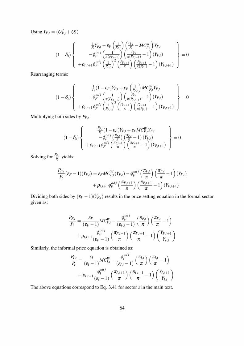
Using YF,t = (QdF,t +Qx

t )

(1−δs)

1Pt

YF,t− εF

(1

PF,t

)(PF,tPt−MCW

F,t

)YF,t

−φad jF

(1

π(PF,t−1)

)(PF,t

π(PF,t−1)−1)(YF,t)

+ρt,t+1φad jF

(1

PF,t

)2(PF,t+1π

)(PF,t+1π(PF,t)

−1)(YF,t+1)

= 0

Rearranging terms:

(1−δs)

1Pt(1− εF)YF,t + εF

(1

PF,t

)MCW

F,tYF,t

−φad jF

(1

π(PF,t−1)

)(PF,t

π(PF,t−1)−1)(YF,t)

+ρt,t+1φad jF

(1

PF,t

)2(PF,t+1π

)(PF,t+1π(PF,t)

−1)(YF,t+1)

= 0

Multiplying both sides by PF,t :

(1−δs)

PF,tPt(1− εF)YF,t + εFMCW

F,tYF,t

−φad jF(πF,t

π

)(πF,tπ−1)(YF,t)

+ρt,t+1φad jF

(πF,t+1

π

)(πF,t+1

π−1)(YF,t+1)

= 0

Solving for PF,tPt

yields:

PF,t

Pt(εF −1)(YF,t) = εFMCW

F,t(YF,t)−φad jF

(πF,t

π

)(πF,t

π−1)(YF,t)

+ρt,t+1φad jF

(πF,t+1

π

)(πF,t+1

π−1)(YF,t+1)

Dividing both sides by (εF −1)(YF,t) results in the price setting equation in the formal sectorgiven as:

PF,t

Pt=

εF

(εF −1)MCW

F,t−φ

ad jF

(εF,t−1)

(πF,t

π

)(πF,t

π−1)

+ρt,t+1φ

ad jF

(εF −1)

(πF,t+1

π

)(πF,t+1

π−1)(YF,t+1

YF,t

)Similarly, the informal price equation is obtained as:

PI,t

Pt=

εI

(εI−1)MCW

I,t−φ

ad jI

(εI,t−1)

(πI,t

π

)(πI,t

π−1)

+ρt,t+1φ

ad jI

(εI−1)

(πI,t+1

π

)(πI,t+1

π−1)(YI,t+1

YI,t

)The above equations correspond to Eq. 3.41 for sector s in the main text.

64

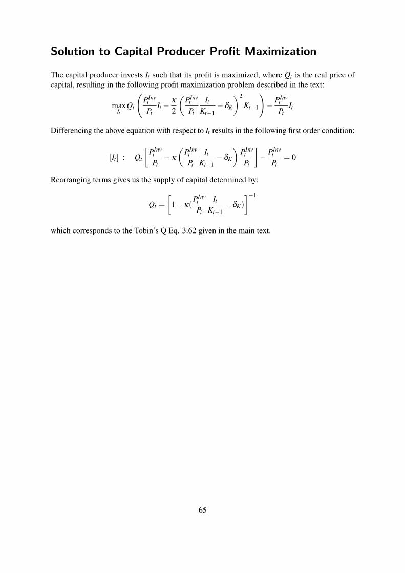
Solution to Capital Producer Profit Maximization

The capital producer invests It such that its profit is maximized, where Qt is the real price ofcapital, resulting in the following profit maximization problem described in the text:

maxIt

Qt

(PInv

tPt

It−κ

2

(PInv

tPt

ItKt−1

−δK

)2

Kt−1

)− PInv

tPt

It

Differencing the above equation with respect to It results in the following first order condition:

[It ] : Qt

[PInv

tPt−κ

(PInv

tPt

ItKt−1

−δK

)PInv

tPt

]− PInv

tPt

= 0

Rearranging terms gives us the supply of capital determined by:

Qt =

[1−κ(

PInvtPt

ItKt−1

−δK)

]−1

which corresponds to the Tobin’s Q Eq. 3.62 given in the main text.

65