Macroeconomic stabilisation policies in the EMU: Spillovers, asymmetries, and institutions ∗ Giovanni Di Bartolomeo University of Rome “La Sapienza” Jacob Engwerda Tilburg University Joseph Plasmans † University of Antwerp and Tilburg University Bas van Aarle University of Leuven and University of Nijmegen June, 2003 Abstract This paper studies the spillover sizes and signs and the institutional design of the co-ordination of macroeconomic stabilisation policies within the European Economic and Monetary Union (EMU). Moreover, in a dynamic setup, the consequences of this institutional design on macroeco- nomic outcomes and policies are analysed. We distinguish two types of co-ordination: ex-ante - related to the institutional framework; and ex-post concerning the actual policy decisions. The first type is modeled as the result of an endogenous coalition formation process that leads to the formation of policymakers’ coalitions. Ex-post co-ordination implies then the implementation by each coalition of its internally co-ordinated macroeconomic stabilisation policies in a non-co- operative dynamic game with the other coalitions, and subject to the constraints of the internal dynamics of the EMU economy. The paper shows that the institutional setting of macroeconomic policy co-ordination is of crucial importance in reaching the Pareto-optimal equilibrium of the game, especially when the number and the magnitude of asymmetries increase. The specific recommendations depend on the particular characteristics of the shocks and the economic structure. In the case of a common shock, fiscal co-ordination is counterproductive but full policy co-ordination is desirable. When asymmetric shocks are considered, fiscal co-ordination improves the performance but full pol- icy co-ordination doesn’t produce further gains in policymakers’ welfare. In general, structural asymmetries reduce the gains from co-operation so that in many cases co-operation cannot be supported without introduction of exogenous factors, e.g. a transfer system. JEL codes: C70, E17, E58, E61, E63. Keywords: Macroeconomic stabilisation, EMU, coalition formation, linear quadratic differential games. 1 Introduction On January 1st 2002, the euro notes and coins have been introduced in 12 EU countries. These are the most tangible signs of the new economic and political regime established by the Economic and ∗ We are grateful to conference and seminar participants at EcoMod 2002 (Brussels), the AFSE Conference on ’Growth, Convergence and European Integration’ (Lille, 2003) and the University of Antwerp for useful comments on the first preliminary version of this paper. We would like to thank Tomasz Michalak for assistance in the final stage of the research. Giovanni Di Bartolomeo acknowledges the financial support from the University of Rome ‘La Sapienza’ (MURST 2000) and the University of Antwerp (Special Research Fund) and Bas van Aarle acknowledges the financial support from the FWO (Fonds voor Wetenschappelijk Onderzoek Vlaanderen). † Corresponding author, Faculty of Applied Economics UFSIA-RUCA, University of Antwerp, Prinsstraat 13, B2000 Antwerp; Phone: +32 (0)3 220 4149, Fax: +32 (0)3 220 4585, Email: [email protected]. 1
Transcript
Macroeconomic stabilisation policies in the EMU: Spillovers,asymmetries, and institutions∗
Giovanni Di BartolomeoUniversity of Rome “La Sapienza”
Jacob EngwerdaTilburg University
Joseph Plasmans†
University of Antwerp and Tilburg University
Bas van AarleUniversity of Leuven and University of Nijmegen
June, 2003
AbstractThis paper studies the spillover sizes and signs and the institutional design of the co-ordination
of macroeconomic stabilisation policies within the European Economic and Monetary Union(EMU). Moreover, in a dynamic setup, the consequences of this institutional design on macroeco-nomic outcomes and policies are analysed. We distinguish two types of co-ordination: ex-ante -related to the institutional framework; and ex-post concerning the actual policy decisions. Thefirst type is modeled as the result of an endogenous coalition formation process that leads tothe formation of policymakers’ coalitions. Ex-post co-ordination implies then the implementationby each coalition of its internally co-ordinated macroeconomic stabilisation policies in a non-co-operative dynamic game with the other coalitions, and subject to the constraints of the internaldynamics of the EMU economy.The paper shows that the institutional setting of macroeconomic policy co-ordination is of
crucial importance in reaching the Pareto-optimal equilibrium of the game, especially when thenumber and the magnitude of asymmetries increase. The specific recommendations depend onthe particular characteristics of the shocks and the economic structure. In the case of a commonshock, fiscal co-ordination is counterproductive but full policy co-ordination is desirable. Whenasymmetric shocks are considered, fiscal co-ordination improves the performance but full pol-icy co-ordination doesn’t produce further gains in policymakers’ welfare. In general, structuralasymmetries reduce the gains from co-operation so that in many cases co-operation cannot besupported without introduction of exogenous factors, e.g. a transfer system.JEL codes: C70, E17, E58, E61, E63.
Keywords: Macroeconomic stabilisation, EMU, coalition formation, linear quadratic differentialgames.
1 Introduction
On January 1st 2002, the euro notes and coins have been introduced in 12 EU countries. These arethe most tangible signs of the new economic and political regime established by the Economic and
∗We are grateful to conference and seminar participants at EcoMod 2002 (Brussels), the AFSE Conference on’Growth, Convergence and European Integration’ (Lille, 2003) and the University of Antwerp for useful comments onthe first preliminary version of this paper. We would like to thank Tomasz Michalak for assistance in the final stage ofthe research. Giovanni Di Bartolomeo acknowledges the financial support from the University of Rome ‘La Sapienza’(MURST 2000) and the University of Antwerp (Special Research Fund) and Bas van Aarle acknowledges the financialsupport from the FWO (Fonds voor Wetenschappelijk Onderzoek Vlaanderen).
†Corresponding author, Faculty of Applied Economics UFSIA-RUCA, University of Antwerp, Prinsstraat 13, B2000Antwerp; Phone: +32 (0)3 220 4149, Fax: +32 (0)3 220 4585, Email: [email protected].
1
Monetary Union (EMU) whose formal operation started on January 1st 1999, after the prolongedpreparation period laid out in the Maastricht Treaty of 1991.
The main institutional change in EMU is clearly the constitution of a common central bank(European Central Bank - ECB). Moreover, fiscal policies are now regulated according to the BroadEconomic Policy Guidelines (BEPGs) established by the European Commission (EC) in 2000 and thedecisions taken within the ECOFIN Council of (Economics and Finance) Ministers (for the wholeEU) and the Eurogroup (for the EMU)1. For example, the fiscal policy of the EU Member Statesis monitored within the framework of the BEPGs by the EC with recommendations, warnings, andjudgements. An example is the ECOFIN Council recommendation to Ireland on the 12th of February2001, addressing the inconsistency between the Irish budget for 2001 and the BEPGs. Other casesare the recommendations with early warnings by the EC for Germany and Portugal on the 11th ofFebruary 2002 and more recently - on the 21st of January 2003 - for France. However, the institutionsand the procedures for economic policy co-ordination are far from being completely established, and,therefore, several matters are still under discussion. Having in mind this context, this paper studiesthe institutional design of the co-ordination of macroeconomic stabilisation policies within the EMUand its consequences on macroeconomic outcomes and policies.
Fiscal policy co-ordination in a monetary union is directly linked to the sizes and signs of thespillovers and externalities resulting from national fiscal policies. The sign and size of fiscal spilloversare crucial since they ultimately determine whether co-ordination should lead to a more expansionaryor a more restrictive fiscal stance in the Member States. For example, if governments perceive negativespillovers in a static game, they would interpret non-co-operative (“beggar-thy-neighbour”) policy inresponse to bad economic shocks as too expansionary and would agree on a more restrictive stance inall countries. By contrast, if governments perceive positive spillovers, co-ordination should eliminatefree-riding behaviour of individual countries and promote more expansionary policy in response tobad economic shocks. In a dynamic setting the situation is more complicated as the size, persistenceand signs of the spillovers may change markedly over time.
The EMU is clearly a highly integrated economic area with a large number of interactions betweenthe participating countries. However, empirical estimations of spillovers in such a context are not(yet) available2 and the theoretical literature does not provide a clear-cut answer about the sign offiscal policy spillovers. The traditional argument in favour of international policy co-ordination isbased on direct positive demand spillovers. By contrast, more recent, micro-founded models of theEMU tend to conclude in favour of negative fiscal spillovers by emphasizing the adverse terms-of-trade effects of balanced-budget foreign fiscal expansion on the domestic economy. Furthermore, thepossibility of accumulating public debts might add other sources of negative spillovers through thecommon nominal interest rate.
In the EMU a central role is played by the co-ordination of the fiscal policies among the nationalgovernments3 and, moreover, their co-ordination with the monetary policy of the ECB. In general,two kinds of co-ordination can be distinguished (Beetsma et al. (2001)): institutional (or ex-ante)co-ordination, and policy (or ex-post) co-ordination.
Ex-ante co-ordination is related to the institutional framework, the co-ordination procedures,and the design of policy rules, whereas ex-post co-ordination takes place from the current state ofaffairs and concerns the actual policy decisions. More in particular, ex-ante co-ordination operatesthrough formal binding agreements recognised by the policymakers as international obligations (e.g.
1The Eurogroup, however, is not officially institutionalised, but is an informal meeting of the Ministers of Financeof the EMU Member States.
2A very preliminary attempt to estimate cross-country spillovers within EMU is provided by Monteforte and Siviero(2003). Moreover, Monfort et al. (2002) try to empirically disentangle common shocks and spillover effects in amulti-country setting.
3 Inflation bias, which may arise in the setting of fiscal policy, is likely to be stronger in a multi-country monetaryunion with nationally-set fiscal policies than in the case of EMU-wide set fiscal policies. It is important, therefore, todesign institutions for commitment and co-ordination of fiscal policies in order to mitigate such biases (CESifo (2002,Chapter 3)).
2
the Maastricht Treaty and the Stability and Growth Pact (SGP)). By contrast, ex-post co-ordinationhas an informal character, and refers to discretionary and ad hoc informal agreements stipulatedamong the countries.4 The two kinds of co-ordination are strictly interconnected. In fact, e.g., theSGP might strongly reduce the room for discretionary co-ordination of the national fiscal policies.Similarly, discretionary agreements among the countries might depend on the design of the Europeaninstitutions concerning fiscal co-operation as, e.g., the ECOFIN Council.
We consider, in a dynamic modelling framework, that foreign fiscal policy can affect the domesticeconomy through the terms-of-trade, the real interest rate, and external demand spillovers. Differentsigns of the spillovers can arise according to different parameterisations of the model. In the contextof co-ordination of macroeconomic stabilisation policies the following topics will be discussed:
1. The assignment issue that consists in deciding which institution is responsible for which policytarget and at which scope. And, in addition to it, which policy tool is assigned to which policyinstitution. It is of particular interest to study the effects of different governments’ priorities ina monetary union where the monetary policy is fully delegated to a unique central bank, whichis mainly associated with price stabilisation (Art. 105 Treaty of European Community, TEC).
2. The institutional framework where both the assignment and the co-ordination are solved (ex-ante co-ordination). In particular, the concept of ex-ante co-ordination is related to the func-tions that should be associated with the Eurogroup and the ECOFIN Council. In fact, differentdegrees of enforcement associated with the ECOFIN Council recommendations and judgementsmight have a crucial effect on macroeconomic policy co-ordination, or on the failure in imple-menting it.
3. The ex-post co-ordination issue among the fiscal authorities and between them and the ECB.This issue in the EMU adds a new feature to the traditional issues related to the public goodnature of price stability and the macroeconomic externalities due to the national fiscal policies.In fact, in the EMU the co-ordination problem is very much focused on enforcing budgetarydiscipline (Art. 104 TEC and the SGP).
Regarding the assignment issue we will consider different priorities for output gap and inflationfor the fiscal and monetary authorities. The governments are mainly concerned with output gapstabilisation whereas the ECB’s primary target (according to Art. 105 TEC) is stability of prices inthe Euro-area. In addition, we introduce deficit stabilisation as an explicit objective of the individualgovernments. By doing this we include the fiscal stringency requirements of the SGP as an elementin the decision making problem of the fiscal authorities. Interest rate smoothing is included in theobjectives of the ECB. In the context of the EMU it is interesting to analyse how such externallyimposed institutional restrictions on policy instruments affect the design of optimal policies andaspects of policy co-operation.
The institutional framework (ex-ante co-ordination) is introduced by considering different rules,procedures and information shared among policymakers, which taken together characterise the nego-tiations among policymakers in determining co-operation agreements. Different institutional settingsmay have different effects on the implementation of co-operative policies. In fact, some institutionalsetups may not be able to promote co-operation, even when co-operative policies increase the welfareof policymakers because of free-riding behaviour.
Ex-post co-ordination will be studied in a dynamic framework to emphasize the dynamic characterof both direct and indirect spillovers arising from the behaviour of national fiscal policies in anintegrated area as the EMU. The direct spillovers from fiscal policies result from the effect of domestic
4As it is pointed out by Beetsma et al. (2001), we can think of the Eurogroup, in which the Finance Ministers ofthe EMU area discuss fiscal policies in an informal way, as a forum of ex-post co-ordination. Furthermore, also theECOFIN Council, notwithstanding its more formal nature, is characterised by largely discretionary decisions and can,therefore, be interpreted as a formal institution where not only formal but also informal agreements take place.
3
output on foreign output via the export channel. The indirect spillovers result from the effects offiscal policies on the dynamics of inflation rates, intra-EMU competitiveness, and interest rates.
Our paper extends the literature in three respects.
(a) From the methodological point of view, this paper extends Di Bartolomeo et al. (2002b) byconsidering a more general shock structure - based on inflation instead of competitiveness - inthe model dynamics. Moreover, more general inflation dynamics are considered: the effects offoreign inflation rates are included, as suggested by the recent open-economies’ literature.5
(b) We explicitly introduce the issue of endogenous coalition formation. More in detail, we use thepartitioned game approach of the endogenous coalition formation literature. This approachconsists in reducing a game in normal form to a two-stage game (a partitioned game). In thefirst stage policymakers try to form coalitions among themselves by playing non-co-operativelyaccording to different possible assumptions (to which correspond different equilibrium con-cepts). Afterwards, in the second stage of the game, the coalitions formed (or the singletons)play non-co-operatively in setting their stabilisation policies to face a macroeconomic shock.However, the partitioned approach has a limitation. Once coalitions are formed, they cannotchange.6 Therefore, binding agreements must be assumed in the second stage of the game.
(c) In this paper we also extend the current literature on the institutional design (ex-ante co-ordination) of the EMU by taking account of a dynamic framework. After solving the n-countrymodel analytically according to the standard linear-quadratic methodology based on the re-duced form of the model, we expose the main features of our model by numerical simulationsbased on structural form parameters. In the numerical simulations, we will analyse the con-sequences of ex-ante and ex-post policy co-ordination under different assumptions on the signand size of the fiscal spillovers, and on the asymmetries among Member States. The differ-ent forms of asymmetry that will be investigated are: countries having asymmetric structuralmodel parameters (model asymmetry), policymakers having different preferences (preferenceasymmetry), and, finally, shocks that asymmetrically hit countries (shock asymmetry).
The paper is organised as follows. Section 2 provides a small dynamic macro-economic model ofthe EMU economy and the dynamic stabilisation problem the fiscal policymakers and the commonmonetary authority are facing. Section 3 discusses in detail the institutional aspects of policy co-ordination in the EMU context and how these aspects are incorporated into our analysis. Section4 analyses the consequences of ex-post and ex-ante policy co-ordination in a dynamic framework bystudying numerical simulations of various examples. An Appendix is added with details on analyticaland computational aspects underlying our analysis.
2 The basic economic framework
In this section we describe our basic framework. We consider a model where n countries (N :={1, 2...n}) participate in a monetary union. Each economy is described by an aggregate demand/IScurve and an aggregate supply curve (derived from a Phillips relationship). All the variables arein logarithms, except for the interest rate which is in perunages, and denote deviations from theirlong-run equilibrium that has been normalised to zero, for simplicity. A dot above a variable denotesits time derivative.
Equations (1) are the IS curves which represent the aggregate demand (AD) in each of the EMUcountries as a function of competitiveness in intra-EMU trade, the domestic real interest rate, the
5Evidence of foreign inflation effects on the Phillips curve is provided by DiNardo and Moore (1999). See also Razinand Yuen (2001) and Di Bartolomeo et al. (2003).
6This is in accordance with the open-loop Nash solution concept utilised in this paper.
4
foreign real output gaps, and the domestic real fiscal deficit. Hence, the aggregate demand satisfies:
xi(t) = −γi [iE(t)− pi(t)] + ηifi(t) +Xj∈N/i
ρijxj(t) +Xj∈N/i
δij [pj(t)− pi(t)] (1)
in which x denotes the real output gap (defined as real output relative to potential real output7), fthe real fiscal deficit, p the price level, and iE the common nominal interest rate in the EMU area.The (expected) real interest rate is defined as the difference between the nominal common interestrate and the (expected) inflation in a country8. Although the nominal interest rate is the same forthe whole Euro area, real interest rates diverge among countries if inflation rates are different.
Equations (2) are open-economy Phillips curves, which describe the aggregate supply (AS) ineach of the EMU countries:
pi(t) = ζixi(t) +Xj∈N/i
ςij pj(t) , pi(0) = pi0 (2)
Aggregate supply is assumed to be determined by a Phillips curve implied by the existence ofsome (nominal) rigidities in the goods (and/or labour) markets giving rise to a short-run trade-offbetween inflation and output. In this Phillips relationship the inflation rates of the other countriesplay a role since it is assumed that a real wage wedge between the real wage relevant for the domesticfirms (based on the producer price index) and that relevant for the trade unions (based on theconsumer price index) exists. In accordance with our short-run stabilisation focus, the effectivenessof fiscal policy is limited to its transitory impact on the output gap through the induced stimulusof the aggregate demand. The initial values of domestic prices represent (initial) level shocks thathit the economy at time zero. In this setting both symmetric and asymmetric price shocks can beconsidered.
Within the above economic framework, we assume that the fiscal authorities control their fiscalpolicy instrument such as to minimise the following quadratic loss function9, which features domesticinflation, real output gap, and real fiscal deficit, with respect to the control variable fi:
Ji(t0) =1
2
∞Zt0
{αip2i (t) + βix2i (t) + χif
2i (t)}e−θ(t−t0)dt (3)
in which θ denotes the rate of time preference and αi, βi, and χi represent preference weights thatare attached to the stabilisation of inflation, output, and fiscal discipline, respectively (in general,βi > αi). In particular, parameter χi is an indicator for the stringency of the rules imposed by theSGP. A higher value of χi in this interpretation means that the SGP is more strictly interpreted andhigh deficits bear high costs.
We choose the EMU-wide nominal interest rate as the ECB’s monetary policy instrument andadd an interest rate smoothing objective in the ECB’s cost function, to express the ECB’s caution insetting monetary policy. Consequently, we assume that the ECB is confronted with the minimisationof the following loss function:
JE(t0) =1
2
∞Zt0
Ã
nXi=1
αiE pi(t)
!2+
ÃnXi=1
βiExi(t)
!2+ χEi
2E(t)
e−θ(t−t0)dt (4)
7 In this paper, it is assumed that the equilibrium real output gap has been normalised to zero for convenience.8We have assumed that expected inflation equals actual inflation in (1). Given the deterministic nature of the model,
this amounts to assuming perfect foresight.9Note that the quadratic form of the loss function implies that policymakers are equally concerned about inflation
and deflation and about a negative output gap vs. a positive one. This may not always be realistic; however, such anassumption is necessary to keep the analysis more tractable.
5
The minimisation of this loss function w.r.t. iE(t) is consistent with the derivation of a standardmonetary policy rule (see e.g. Clarida et al. (1999)), since it results in a linear function in itsarguments.
The structural form model (1)-(2) can be transformed into the following reduced form model:10
·x(t)p(t)
¸=
·D E MA B N
¸ p(t)f(t)iE(t)
(5)
where x(t) is a country-ordered vector of output gaps, p(t) is a country-ordered vector of inflationrates, p(t) and f(t) are the price level and fiscal deficit vectors, respectively.11 The partitioned matrix
L :=
·D E MA B N
¸indicates the elasticities of the real output gap and inflation with respect to price
levels and control instruments. The upper part of matrix L ∈ IR2n×(2n+1) indicates the instantaneouselasticities of the real output gaps. The lower part of this matrix indicates the elasticities of theinflation dynamics of the model. The matrix L is crucial in the analysis of the externalities. More indetail, the matrix E ∈ IRn×n describes the effects of the domestic fiscal policy on the domestic realoutput gaps (main diagonal elements) and those of the foreign fiscal policies on the domestic realoutput gaps (off-diagonal elements); the latter elasticities are called fiscal externalities. Similarly, thematrix B ∈ IRn×n describes the effects of the fiscal policy variables on the inflation rates. MatricesD ∈ IRn×n and A ∈ IRn×n indicate the effects of domestic and foreign price levels on the domestic realoutput gaps and inflation rates, respectively. Vectors M ∈ IRn and N ∈ IRn are the semi-elasticitiesof the real output gaps and inflation rates w.r.t. to the common nominal interest rate.
3 Externalities and the institutional setup
3.1 Shocks and externalities
In most cases the debate on the desirability of international policy co-ordination focuses on themagnitude and the signs of the fiscal spillovers that could justify a more co-operative approach todemand-oriented fiscal policies. A further (recently introduced) aspect is related to the action of theECB, which can neutralise the effects of fiscal co-operation if its targets are opposed to those of thenational governments (see Beetsma and Bovenberg (1998) and Acocella and Di Bartolomeo (2001)).
The sign and size of fiscal externalities are particularly important as they ultimately determinehow large such effects of fiscal spillovers are (in absolute terms) and whether co-ordination shouldlead to a more expansionary or more restrictive fiscal stance in the Member States (Beetsma et al.(2001), pp. 4-5).
The theoretical literature does not provide a clear-cut answer about the sign of these externalities.The main channels of the effects of the domestic fiscal expenditure externalities on foreign real outputgaps are from the terms of trade (negative), the real interest rate (negative), and external demand(positive) spillovers (Levine and Brociner (1994)). Overall, the validity of the argument in favour ofnegative externalities primarily depends on the empirical importance of intra-EMU terms-of-tradeeffects and on the reaction of the common interest rate to changes in fiscal policy. In most of thetheoretical models, terms-of-trade effects are significant because they implicitly assume strategicinteraction(s) within a group of large countries making up the world economy. However, accordingto Beetsma et al. (2001), the EMU is better described as a club of small economies open to therest of the world. More specifically, the goods exchanged among EU Member States are also tradedat the world level, a level at which individual EU economies can be assumed to be small in thetrade-theoretic sense.10See the Appendix for the derivation of the reduced form of the model.11Clearly, the dimension of all these vectors is n.
6
Fiscal policy affects not only domestic and foreign real output gaps but also domestic and foreigninflation. Therefore, externalities may also emerge from the fiscal authorities’ behaviour through theinflation channel. Fiscally-induced inflation externalities also raise a new issue in the EMU context,namely the interplay of the ECB with the national fiscal authorities and possible conflicts associatedwith different policymakers’ preferences. Moreover, many of the results of the policy co-ordinationliterature based on two-country models (the “two-is-many” principle) are not valid when a thirdplayer is considered (see Rogoff (1985) and Kehoe (1989)). In our context, the natural “third player”is the ECB12 and, considering the explicit separation of monetary and fiscal authorities, conflictsamong the national governments about the orientation of the macroeconomic policy mix are ofteninevitable.13 A potentially large discrepancy between the objectives of the ECB and those of thenational governments is a serious and permanent source of tension, in addition to possible conflictsdue to different cyclical or structural conditions (see Debrun (2000) and Acocella and Di Bartolomeo(2001)).
Besides the interpretation of the matrix L as a matrix of externalities, the initial shock structurehas to be taken into account. Actually, each policymaker reacts to an initial shock. However, thepolicy actions also affect the other countries and imply a feedback from them. This feedback willbe determined by the effects of the monetary and fiscal policies from the other countries and theseeffects are captured by matrix L too.
3.2 Institutional setup and co-operative mechanisms
The current policy framework of the EMU presents a strong asymmetry between the managementof fiscal and monetary policies. The common monetary policy is determined by a supranationalpolicymaker (the ECB) with a statutory primary objective, achieving and maintaining price stabilityin the EMU area. On the contrary, fiscal policies remain in the hands of the Member States, with noobjective specified by the Treaty but constrained by the SGP-requirements. This decentralised man-agement of the fiscal policies raises several issues on the need of ex-post co-ordination among MemberGovernments and the eventual alternative mechanisms that can guarantee ex-ante co-ordination.14
The ex-ante co-ordination among fiscal policymakers can be implemented according to positiveor negative mechanisms. In the EU the only positive mechanism for fiscal policy co-ordination(positive co-ordination) is the use of the BEPGs, which, however, are mostly used as non-bindingrecommendations prepared by the EC and adopted by the ECOFIN Council each year. Assumingnegative fiscal externalities, a negative mechanism for fiscal co-ordination (negative co-ordination) isbased on the sanctions in the case of excessive deficits from the SGP. The SGP allows the ECB to“play on the safe side” by putting a strong limit to the discretional power of the national governmentsin setting their independent fiscal policies (Onorante (2002)).
In the ongoing debate, it is argued that increased co-ordination should include 1) a greater sharingof information among the Member States, 2) a greater positive co-ordination, and 3) a progressivereduction of the importance of negative (rule-based) co-ordination.15
In this paper the institutional design issue and ex-ante positive co-ordination are introduced byassuming that policymakers, who face a stabilisation problem in the EMU, play a two-stage game. Inthe first stage (the coalition game) they decide non-co-operatively whether or not to co-ordinate theirfiscal policies after that common or country-specific shocks have been observed. In the second stage
12See e.g. Agell et al. (1996), Jensen (1996), Beetsma and Bovenberg (1998), and Acocella and Di Bartolomeo (2001).13According to Beetsma et al. (2001), p. 6, "such conflicts are particularly relevant in the European context where
the central bank has a mandate to focus primarily on price stability. This is certainly narrower than the mandate givento the national governments by their electoral constituencies."14Although several studies have investigated the effects of (needs for) fiscal and/or monetary co-ordination, only a
few have challenged the issue of the co-ordination mechanism by comparing alternative schemes (see e.g. van Aarle etal. (2002a) and Onorante (2002)).15These guidelines are however not fully agreed. For example, Uhlig (2002) claims that SGP needs strengthening
rather than weakening (so he calls for an increase of negative co-ordination).
7
(the stabilisation game) they play a non-co-operative dynamic game, where those policymakers, whohave signed the agreement, play as a single player sharing a common loss function. The rules of thefirst-stage game determine the institutional setup (ex-ante co-ordination) whereas the second stageof the game describes ex-post co-ordination. According to the rules determined in the institutionalco-ordination negotiations, different coalition structures may emerge when ex-post co-ordination isconsidered. Negative co-ordination is determined by the magnitude of the costs associated with thefiscal stance prescribed by the SGP.
In the first stage of the game, we restrict our attention to four alternative institutional settings.Different setups are associated with different stylised institutional setups characterised by differentbargaining powers, procedures, rules, and available information among policymakers.16
1. We first consider an equilibrium where decisions about fiscal policies are determined by the na-tional governments and fiscal co-ordination is arranged by multilateral agreements determinedaccording to the following procedure. All policymakers simultaneously face the problem ofaccepting or rejecting a proposal that consists in sharing their loss functions when setting theirfiscal policies. After that all agents’ decisions are taken, the equilibrium is formed. In gametheory this equilibrium concept is formalised as the Coalitional Nash Equilibrium (CNE).17
This institutional setup is probably the closest to the current institutional setting of the EMUbased on decentralised fiscal policymakers.
2. Second, we consider an institutional setup driven by an equilibrium where decisions abouteconomic policies are determined entirely at the EMU level by an institutionalised and cen-tralised Eurogroup, which decisions are binding for the national governments (full co-operationsetup with co-ordination of fiscal and monetary policies; the corresponding full-co-operativeequilibrium is denoted by C).
3. Third, we assume that decisions about fiscal policies are determined by the national gov-ernments and that co-ordination is built on the basis of a hierarchical sequential negotiationprocess (Sequential Negotiation Equilibrium, SNE).18 This mechanism emphasizes the possiblerole played by single countries in the negotiation for achieving a co-ordination agreement, e.g.that with the temporary EU President Country. In this case, the EU Presidency determines alist of proponents (list of order) among the Member Country Ministers, and then each minister,according to this list of order, proposes a coalition to a group of countries. Countries that ac-cept a proposal exit from the game. An equilibrium of such a negotiation scheme is an SNE. Inthe Appendix we describe an algorithm for the computation of a unique SNE. This mechanism
16See van Aarle et al. (2002b) for a first exploratory treatment of these (dynamic) coalitional equilibria concepts.17The CNE is the most common Nash equilibrium concept in the coalition formation literature. It was first introduced
by the seminal studies of d’Aspremont et al. (1983) in the industrial organization literature. A CNE is an equilibrium ofa one-shot game where each agent faces the problem of simultaneously accepting or rejecting a proposal that consists insharing her utility function only by looking at the immediate consequence of her actions. After that all agents’ decisionsare taken, the CNE is formed. This equilibrium is fully characterised by the fulfilment of two stability conditions anda profitability condition. The stability conditions assure that no policymaker has an incentive in deviating from itsstrategy by entering in an existing coalition (external stability) or leaving an existing coalition (internal stability).Profitability means that the coalition members incur a loss which is lower than that they would get when all playerswould act as singletons (i.e. when they play non-co-operatively).18See e.g., Bloch (1996) and Ray and Vohra (1999). An SNE is an equilibrium of a hierarchical multi-stage negotiation
process. The negotiation starts with one policymaker who proposes a coalition. The order of agents that can propose acoalition is given by an exogenous rule (i.e. a rule of order). Each prospective member can reject or accept the proposalin the order determined by this fixed rule. If one of the policymakers rejects the proposal, that policymaker must makea counter-offer. If all members accept, the coalition is formed and then all members of that coalition withdraw from thenegotiations. When all agents exit from the negotiation the SNE is formed. Hence, one player after the other decidesto propose a coalition to the other players. These decisions are determined by non-cooperative best-reply rules, giventhe coalition structure and the allocation in the previous rounds. One of the nice features of this approach is that itmight explain in terms of history why specific stable coalitions are reached among the many possible ones. In otherwords, the importance of historical relationships between nations might be captured by this approach.
8
has, however, several drawbacks. The most important of them is that the outcome can dependon the list of order, and, therefore, an institutional question arises: ‘Who determines that list,since the list order can be chosen strategically in order to determine a possible coalition?’
4. Finally, we consider the possibility of reaching final decisions about co-ordination on the basisof a sequentially repeated negotiation process that ends when there are no further opportuni-ties of gains for the players (Farsighted Coalitional Equilibrium, FCE).19 This equilibrium issupported by an institutional framework where a lot of information circulates among EU poli-cymakers. The importance of information sharing among the EU Member States to implementco-ordination is stressed by Onorante (2002). Moreover, it is also related to the ECB trans-parency. In fact, notwithstanding the ECB’s own insistence about its transparency20, a debatepersists on the level of its accountability and transparency (see e.g. Issing (1999)). Specifically,this equilibrium implies that Member States and the ECB can forecast the reactions of (the)other policymakers to their actions, given that they have enough information about the otherpolicymakers’ preferences and about the state of the whole EMU area.
To summarise, the role played by single countries is ultimately determined by the institutionalrules which govern the EMU. In our model, the ex-ante co-ordination problem takes the form of theendogenous coalition formation process introduced above. The imposition of the fiscal and mone-tary stringency rules provided by the SGP and the Maastricht Treaty clearly leads the institutionalframework and constrains the fiscal and monetary policies. As discussed in Section 2, these require-ments (and the degree of strictness with which they are interpreted) are introduced in the variouspolicymakers’ objectives.
4 Numerical solutions of the model
As a consequence of fixed bilateral exchange rates, asymmetric shocks have long been seen as themajor problem for the EMU (see Favero et al. (2000)). It is generally argued that this kind ofexternalities can be coped by structural reforms that have been advocated to improve flexibility onproduct and labour markets. However, an alternative way resides in the adoption of co-ordinatedpolicies among EU Member countries. In our model different forms of asymmetry can be considered:countries may have asymmetric structural model parameters (model asymmetry), policymakers mayhave different preferences (preference asymmetry), policymakers may have different bargaining powersin negotiating co-operative agreements (power asymmetry) and, finally, shocks may asymmetricallyhit countries (shock asymmetry).
When analysing the different cases of asymmetries, we may compare the positions of e.g. Butiand Sapir (1998) and Beetsma et al. (2001), but now in a dynamic and possibly asymmetric modelsetting. Buti and Sapir (1998) argue that fiscal co-ordination is desirable when large symmetricshocks are present, while Beetsma et al. (2001) argue that fiscal co-ordination is desirable whenthere are asymmetric shocks, because fiscal authorities can internalise opposite fiscal policies whentrying to offset each other’s effect.21 In our numerical simulations, we will consider several of the
19More in detail, the FCE is a multi-stage negotiation procedure based on the idea of indirect domination, whichimplies farsightedness (see e.g. Chwe (1994) and Mariotti (1998)). The indirect domination concept captures the ideathat each agent (or coalition of agents), who deviates from a given coalition structure, has anticipated further deviationsof the other agents. Hence, an FCE is defined as an equilibrium where players foresee the reaction of the other playersto their actions.More information (including specific mathematical properties) on the various equilibrium concepts discussed in this
paper can be found in Di Bartolomeo et al. (2002a).20See e.g. ECB (1999), p.43.21Note also that the analyses of Buti and Sapir (1998) and Beetsma et al. (2001) are mainly limited to ex-post
co-ordination in a static setting only.
9
above mentioned asymmetries; however, we start by describing our benchmark model: a symmetricthree-country model.22
4.1 Symmetric benchmark model
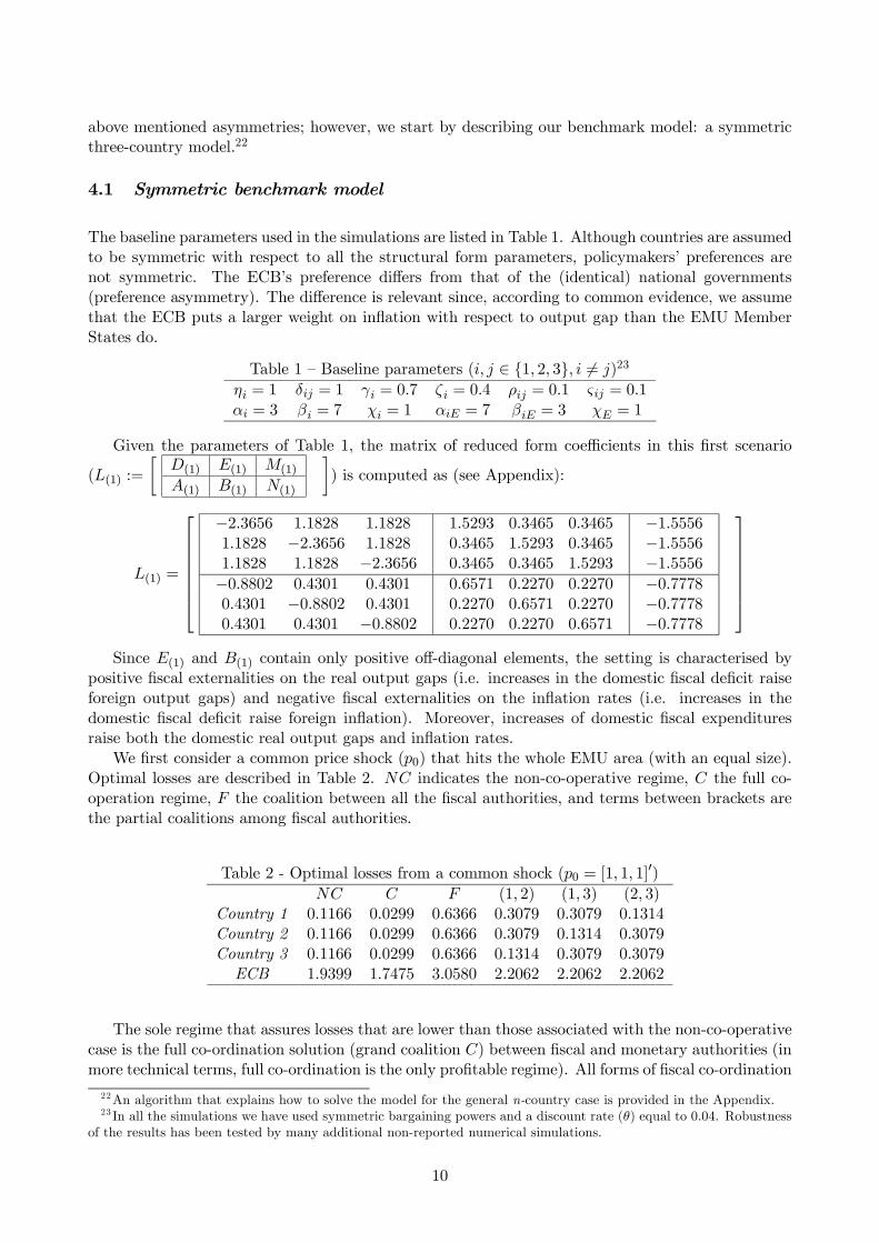
The baseline parameters used in the simulations are listed in Table 1. Although countries are assumedto be symmetric with respect to all the structural form parameters, policymakers’ preferences arenot symmetric. The ECB’s preference differs from that of the (identical) national governments(preference asymmetry). The difference is relevant since, according to common evidence, we assumethat the ECB puts a larger weight on inflation with respect to output gap than the EMU MemberStates do.
Since E(1) and B(1) contain only positive off-diagonal elements, the setting is characterised by
positive fiscal externalities on the real output gaps (i.e. increases in the domestic fiscal deficit raiseforeign output gaps) and negative fiscal externalities on the inflation rates (i.e. increases in thedomestic fiscal deficit raise foreign inflation). Moreover, increases of domestic fiscal expendituresraise both the domestic real output gaps and inflation rates.
We first consider a common price shock (p0) that hits the whole EMU area (with an equal size).Optimal losses are described in Table 2. NC indicates the non-co-operative regime, C the full co-operation regime, F the coalition between all the fiscal authorities, and terms between brackets arethe partial coalitions among fiscal authorities.
Table 2 - Optimal losses from a common shock (p0 = [1, 1, 1]0)
The sole regime that assures losses that are lower than those associated with the non-co-operativecase is the full co-ordination solution (grand coalition C) between fiscal and monetary authorities (inmore technical terms, full co-ordination is the only profitable regime). All forms of fiscal co-ordination
22An algorithm that explains how to solve the model for the general n-country case is provided in the Appendix.23 In all the simulations we have used symmetric bargaining powers and a discount rate (θ) equal to 0.04. Robustness
of the results has been tested by many additional non-reported numerical simulations.
10
are associated with negative performances (i.e. coalition members have losses higher than those thatthey achieve in the complete non-co-operative regime), so they are non-profitable. In this symmetriccase, negative fiscal externalities prevail and partial co-ordination of fiscal policies has a negativeeffect. It is easily verified that all the coalitional equilibria coincide and that the full co-operativecase C is the single equilibrium; hence, CNE=SNE=FCE= C.24
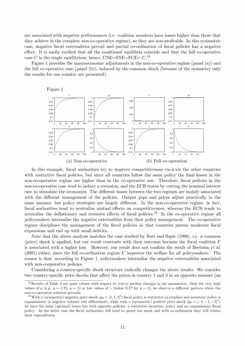
Figure 1 provides the macroeconomic adjustments in the non-co-operative regime (panel (a)) andthe full co-operative case (panel (b)), induced by the common shock (because of the symmetry onlythe results for one country are presented).
Figure 1
0 20 40 60 80 100-0.12
-0.1
-0.08
-0.06
-0.04
-0.02
0f
0 20 40 60 80 100-0.12
-0.1
-0.08
-0.06
-0.04
-0.02
0iE
0 20 40 60 80 100-0.12
-0.1
-0.08
-0.06
-0.04
-0.02
0y
20 40 60 80 1000
0.2
0.4
0.6
0.8
1p
(a) Non-co-operative
0 20 40 60 80 1000
0.02
0.04
0.06
f
0 20 40 60 80 100-0.12
-0.1
-0.08
-0.06
-0.04
-0.02
0iE
0 20 40 60 80 100-0.12
-0.1
-0.08
-0.06
-0.04
-0.02
0y
1 21 41 61 810
0.2
0.4
0.6
0.8
1p
(b) Full co-operation
In this example, fiscal authorities try to improve competitiveness vis-à-vis the other countrieswith restrictive fiscal policies, but since all countries follow the same policy the final losses in thenon-co-operative regime are higher than in the co-operative one. Therefore, fiscal policies in thenon-co-operative case tend to induce a recession, and the ECB reacts by cutting the nominal interestrate to stimulate the economies. The different losses between the two regimes are mainly associatedwith the different management of the policies. Output gaps and prices adjust practically in thesame manner, but policy strategies are largely different. In the non-co-operative regime, in fact,fiscal authorities tend to neutralize mutual effects on competitiveness, whereas the ECB tends toneutralize the deflationary and recessive effects of fiscal policies.25 In the co-operative regime allpolicymakers internalise the negative externalities from their policy management. The co-operativeregime disciplines the management of the fiscal policies so that countries pursue moderate fiscalexpansions and end up with small deficits.
Note that the above analysis matches the case studied by Buti and Sapir (1998), i.e. a common(price) shock is applied, but our result contrasts with their outcome because the fiscal coalition Fis associated with a higher loss. However, our result does not confirm the result of Beetsma et al.(2001) either, since the full co-ordination regime C improves the welfare for all policymakers. Thereason is that, according to Figure 1, policymakers internalise the negative externalities associatedwith non-cooperative policies.
Considering a country-specific shock structure radically changes the above results. We considertwo country-specific price shocks that affect the prices in country 1 and 3 in an opposite manner (an
24Results of Table 2 are quite robust with respect to ceteris paribus changes in the parameters. Only for very highvalues of ρ (e.g. ρ = 1.73, η = 1) or low values of γ (below 0.17 for η = 1), we observe a different pattern where thenon-co-operative solution prevails.25With a (symmetric) negative price shock (p0 = [1, 1, 1]
0) fiscal policy is restrictive (a surplus) and monetary policy isexpansionary (a negative interest rate differential), while with a (symmetric) positive price shock (p0 = [−1,−1,−1]0),we have the same (optimal) losses but with opposite policies: a restrictive monetary policy and an expansionary fiscalpolicy. In the latter case the fiscal authorities will tend to spend too much and with co-ordination they will reducetheir expenditures.
11
asymmetric country-specific shock). Optimal losses for the various regimes are reported in Table 3.
Table 3 — Country-specific shock (p0 = [1, 0,−1]0)NC C F (1, 2) (1, 3) (2, 3)
The most evident feature of Table 3 is that there are no differences in optimal losses between thegrand coalition C, the full fiscal coalition F, and the partial coalition (1, 3). This occurs because thefiscal policy of the first country is exactly offset by the fiscal policy of the third country, due to themodel symmetry and the preference symmetry among fiscal authorities.26 More in detail, in regimeswhere countries 1 and 3 are either both in the same coalition or both outside, due to the equal sizesof the perfectly opposite shocks, the ECB does not affect the dynamics of the game since changes inthe common nominal interest rate equally affect all the prices and output gaps. Results dramaticallychange when partial fiscal coalitions with country 2 are formed, even in this symmetric setting. Withthe partial fiscal coalitions (1, 2) and (2, 3) all the players, including the ECB, are directly affectedin their optimal policies and losses. Coalitions including both countries 1 and 3 are clearly equilibriaof the game since they correspond to the first best strategies for all the players. Hence, SNE= C,CNE= C,F, (1, 3) and the Rational Feasible Coalitions set of FCE = C,F, (1, 3).27
Figure 2 shows the paths of the control variables after the country-specific shock. Again sym-metries have a neutralising effect and tend to compensate the effects of the policymakers’ actions.Co-operation helps in reducing the losses from too expansionary (restrictive) fiscal policies: in theco-operative case country 1 has a smaller deficit and country 3 a smaller surplus than in the non-cooperative case. In this way negative fiscal externalities are internalised and, therefore, partiallyreduced. Because of the perfect structural symmetry of the model, country 2 and the ECB are notaffected at all by the shocks in country 1 and 3.
Figure 2
0 20 40 60 80 100-3
-2
-1
0
1
2
3f1
0 20 40 60 80 100-3
-2
-1
0
1
2
3f2
0 20 40 60 80 100-3
-2
-1
0
1
2
3f3
0 20 40 60 80 100-0.5
0.5iE
0 20 40 60 80 100-3
-2
-1
0
1
2
3f1
0 20 40 60 80 100-3
-2
-1
0
1
2
3f2
0 20 40 60 80 100-3
-2
-1
0
1
2
3f3
0 20 40 60 80 100-0.5
0.5iE
(a) Non-co-operative regime (b) Full and fiscal co-operation regimes
26See van Aarle et al. (2002a) for a more detailed description of this mechanism in a two-country model.27The full coalition C is the sole SNE equilibrium of the game as it is assumed according to the algorithm in the
Appendix that in case of equal losses the players will choose that coalition that contains the highest number of players.A similar reasoning can be applied for the FCE, where it is assumed that in the case where the Rational FeasibleCoalitions set consists of more than one regime, the players will look for an exogenous system to choose the finalcoalition (see the algorithm to compute SNE and FCE equilibria in the Appendix).
12
Notice that the asymmetric country-specific shock analysed in Table 3 is the case which Beetsmaet al. (2001) analyse and find that fiscal co-ordination is desirable. We confirm their result: fiscalauthorities internalise the negative effects of opposite policies with co-ordination. But, we also findthat, in this symmetric setting, no further gains are associated with full co-operation C, which isconfirmed by Figure 2 (no more effects to internalise).
The above model seems to advocate a need for co-ordination. We can distinguish two cases.First, when a common price shock is considered, full co-ordination of economic (monetary and fiscal)policies is required to internalise the externalities. Second, when country-specific shocks occur, co-ordination needs become weaker since only fiscal co-ordination among countries, hit by the shocks,is needed.
However, the above results are based on a reduced form characterised by L(1). Taking a differentset of parameters into account, where e.g. negative fiscal externalities on real output gaps areconsidered instead of positive ones, we obtain a more robust picture of the above results. Assumingς ij = 0.6 (for all i and j ∈ {1, 2, 3} with i 6= j), we get a different reduced form L(2) where E(2) is
, and therefore, negative fiscal externalities with respect toreal output gaps hold. In this and several other (non-reported) simulations, we observed that thefindings of Table 2 are quite robust even if negative fiscal externalities dominate28 (which seems tobe the case in the EMU, although caution needs to be expressed since little econometric evidence isavailable (see footnote 2)).29
4.2 Ex-ante co-ordination (symmetric setting)
In the benchmark model of section 4.1 we have discussed mainly ex-post policy co-ordination inour numerical simulations. Now, we want to study the consequences of different forms of ex-anteco-ordination in more detail.
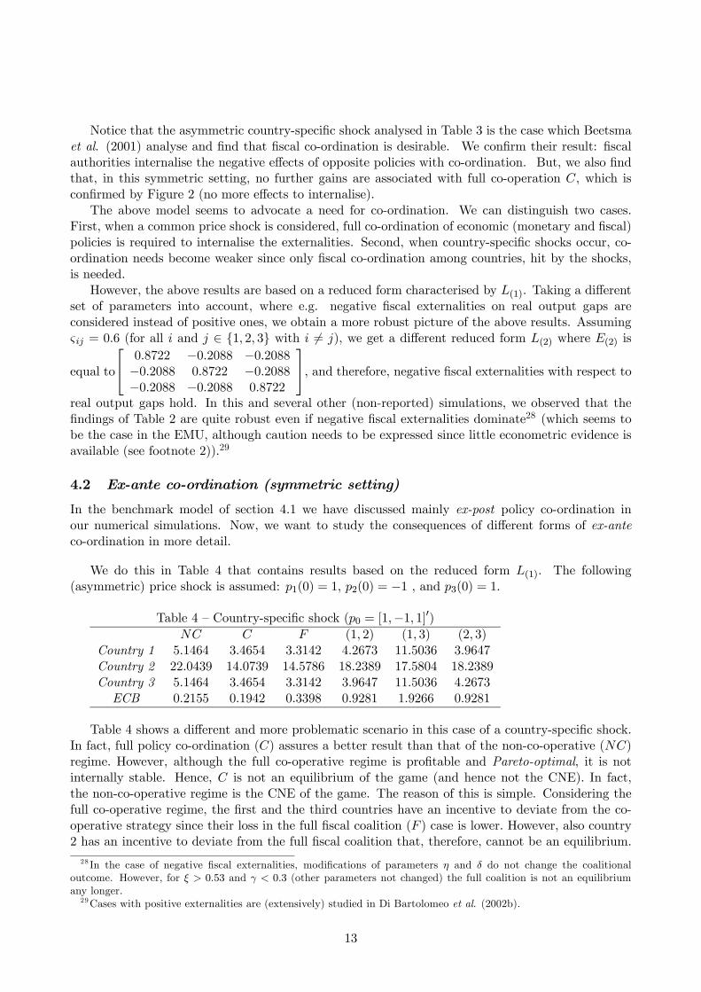
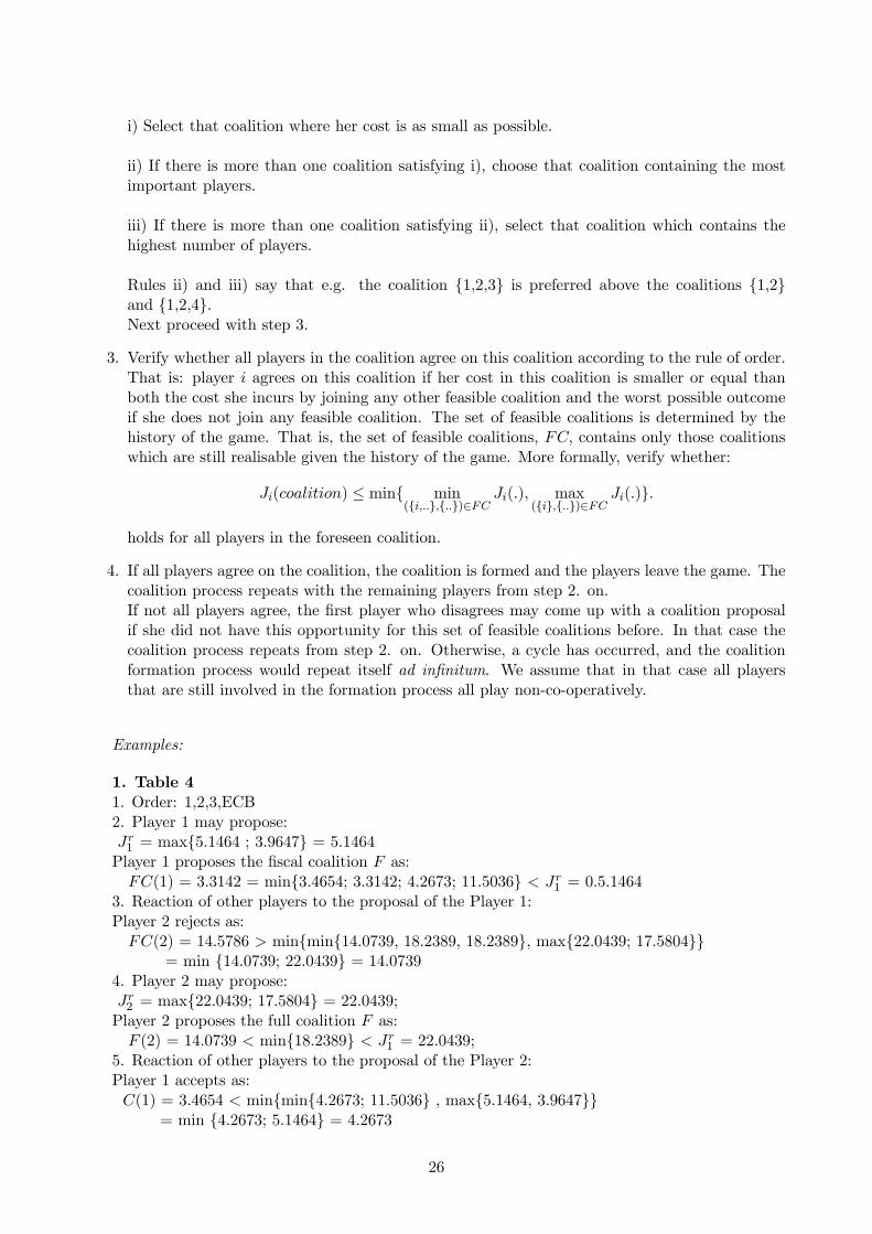
We do this in Table 4 that contains results based on the reduced form L(1). The following(asymmetric) price shock is assumed: p1(0) = 1, p2(0) = −1 , and p3(0) = 1.
Table 4 — Country-specific shock (p0 = [1,−1, 1]0)NC C F (1, 2) (1, 3) (2, 3)
Table 4 shows a different and more problematic scenario in this case of a country-specific shock.In fact, full policy co-ordination (C) assures a better result than that of the non-co-operative (NC)regime. However, although the full co-operative regime is profitable and Pareto-optimal, it is notinternally stable. Hence, C is not an equilibrium of the game (and hence not the CNE). In fact,the non-co-operative regime is the CNE of the game. The reason of this is simple. Considering thefull co-operative regime, the first and the third countries have an incentive to deviate from the co-operative strategy since their loss in the full fiscal coalition (F ) case is lower. However, also country2 has an incentive to deviate from the full fiscal coalition that, therefore, cannot be an equilibrium.28 In the case of negative fiscal externalities, modifications of parameters η and δ do not change the coalitional
outcome. However, for ξ > 0.53 and γ < 0.3 (other parameters not changed) the full coalition is not an equilibriumany longer.29Cases with positive externalities are (extensively) studied in Di Bartolomeo et al. (2002b).
13
For the same reason, partial coalitions cannot be an equilibrium so, notwithstanding its inefficiency,the non-co-operative regime is the sole CNE of the game.
Since theNC-solution is Pareto-inferior with respect to most coalitional outcomes, it is interestingto look for different mechanisms that support co-ordination. The inefficiency that emerges fromTable 4 is related to the mechanism considered in the coalition formation. Different mechanisms caneliminate it. The institutional co-operative design where policymakers act determines the rules ofthe coalition formation process (Ecchia and Mariotti (1997)). For instance, using the algorithm ofthe Appendix for the SNE the resulting equilibrium will be the full policy co-operative equilibrium(C) since each proponent has an interest in proposing full policy co-ordination because it is the onlyone that will be accepted by the others. In other words, countries 1 and 3 know that in this casethe full fiscal coalition (F ) will never be proposed; therefore, they will accept the grand coalitionthat assures a lower loss than that associated with the non-co-operative regime. Also, the FCE ofthe dynamic game includes the full co-operative regime (see the Appendix for details)30. However, amechanism which implies the FCE requires more information than one that supports the SNE or theCNE. For instance, the FCE is not compatible with a central bank that is not transparent or with anenvironment where credible information about the state of the economies of the Member Countriesis not available. If the same Member States have to provide information about their economy theycan try to use this information strategically, and, therefore, the FCE may not characterise such asituation (a similar observation can be made for information provided by the ECB).
Our last example stresses that, even when co-ordination gains are present, co-operative solutionsdo not necessarily emerge as an equilibrium of the game. Different institutional setups (ex-anteco-ordination) imply different equilibria. Therefore, rules, procedures and available information aresometimes crucial to improve co-operative solutions and to raise the welfare of all the policymakersavoiding a free-riding behaviour. Table 4 emphasizes the relevance of the institutional setting de-sign. According to the traditional CNE-mechanism, free-rider behaviour can lead to non-co-operativesolutions (even if co-operation is Pareto-superior to non-co-operation). Hence, co-ordination mecha-nisms become more important. Various alternative (equilibrium) co-ordination mechanisms can beproposed to support co-operation: full co-operation (C), an SNE-mechanism (hierarchical), and anFCE-mechanism (farsighted). It is clear that the C-regime in Table 4 is SNE. The FCE algorithmdoes not provide a clear-cut answer, as the final set of Rational Feasible Coalitions for all playersconsists of both the C-and FC-regimes. Therefore, the final choice between these two regimes de-pends on exogenous factors as e.g. transfer system (see the Appendix for details on computations ofequilibria).
Negotiation mechanisms and their outcomes are clear in the above example. However, less trivialcases may arise when more asymmetries are considered.
The parameters of Table 5 can be interpreted as a setup where a large country (country 1) facestwo small countries that are very sensitive to price changes. In addition, country 3 also importsinflation from the other countries (ς31 = ς32 = 0.2). In such a context we consider the followingcountry-specific price shock: p1(0) = 1, p2(0) = 0.75 , and p3(0) = 0.5.
30The set of Rational Feasible Coalitions in the FCE algorithm consists of the C- and F -regimes. The final outcomedepends on exogenous factors like e.g. the existence of a transfer system.
The reduced form which corresponds to Table 5 (L3) is characterised by the following matrix,that features positive fiscal spillovers for output gaps and negative ones for inflation:
Figures 3 and 4 display the adjustments of control and outcome variables in the non-co-operativeand co-operative regimes. In the non-co-operative regime country 1 has a very expansionary policysince its output is now less affected by the terms of trade, whereas country 3 pursues a comparativelyvery restrictive fiscal policy, as an inflation importer. Country 2 is in between them, with initiallyexpansionary fiscal policy, that eventually turns into a restrictive one.
Under full co-operation the policies follow practically the same pattern as in the non-co-operativecase, but the intensity is more limited due to the internalisation of policy externalities. Especially theECB turns up to be much less active in the interest-rate management. Since countries 1 and 2 havemore limited expansionary fiscal policies, country 3, as an inflation importer, is able to pursue a lessrestrictive (anti-inflationary) fiscal policy. This is, however, optimal from the welfare perspective,which heavily penalises large fluctuations in the price level, like the rapid disinflation that occurs in
15
the non-cooperative regime.
Figure 3 — Adjustments (controls)
0 20 40 60 80 100-0.5
-0.3
-0.1
0.1
0.3
0.5f1
0 20 40 60 80 100-0.5
-0.3
-0.1
0.1
0.3
0.5f2
0 20 40 60 80 100-0.5
-0.3
-0.1
0.1
0.3
0.5f3
0 20 40 60 80 100-0.5
-0.3
-0.1
0.1
0.3
0.5iE
0 20 40 60 80 100-0.5
-0.3
-0.1
0.1
0.3
0.5f1
0 20 40 60 80 100-0.5
-0.3
-0.1
0.1
0.3
0.5f2
0 20 40 60 80 100-0.5
-0.3
-0.1
0.1
0.3
0.5f3
0 20 40 60 80 100-0.5
-0.3
-0.1
0.1
0.3
0.5iE
(a) Non-co-operative regime (b) Full co-operative regime
The large country 1 faces the strongest negative price shock what causes the highest initial decline
in the output. The case of country 3 is interesting, since its output grows initially due to greatercompetitiveness of domestic products caused by higher inflation rates in countries 1 and 2 (negativefiscal externalities). In the process of time, a restrictive fiscal policy, introduced partially due toinflation importing, makes the output gap in this country negative. In the co-operative case, a lessrestrictive policy of the ECB causes inflation in all countries to decline at a slower rate.
Figure 4 — Adjustments (outcomes)
10 20 30 40 50 60 70 80 90 100-0.3
-0.25
-0.2
-0.15
-0.1
-0.05
0
0.05
0.1
0.15
0.2
0.25
0.3y
y1y2y3
10 20 30 40 50 60 70 80 90 1000
0.1
0.2
0.3
0.4
0.5
0.6
0.7
0.8
0.9
1p
p1p2p3
10 20 30 40 50 60 70 80 90 100-0.3
-0.25
-0.2
-0.15
-0.1
-0.05
0
0.05
0.1
0.15
0.2
0.25
0.3y
y1y2y3
10 20 30 40 50 60 70 80 90 1000
0.1
0.2
0.3
0.4
0.5
0.6
0.7
0.8
0.9
1p
p1p2p3
(a) Non-co-operative regime (b) Full co-operative regime
It is easily verified that all the coalitional equilibria coincide and that the full co-operative case Cis the single equilibrium (as being Pareto-superior), hence CNE=SNE=FCE = C (see the Appendixfor details on computations of equilibria).
Table 7, based on the parameters of Table 5 (except for ,ρ12 = ρ13 = 0.04 and ρ21 = ρ23 = ρ31 =ρ32 = 0.01) describes the case of very low positive fiscal externalities from the demand side of theeconomy on the output gap, that is introduced by (rather drastic) changes in the parameter ρ. The
This table shows that the fiscal spillovers have crucial importance for coalition outcomes of thegame. Now, in contrast to the previous case, the non-cooperative regime is the only equilibrium ofthe game, as no coalition is profitable. Out of the institutional designs for co-operation examinedhere, none is able to promote policy co-ordination. The sole way to support full co-operation could beby introducing a transfer system: as countries 1, 2 and the ECB are better off in the full co-operativeregime, they could agree to a transfer towards country 3 to compensate its losses from participatingin the full co-operation equilibrium. However the study of such a transfer system is beyond the scopeof this paper.
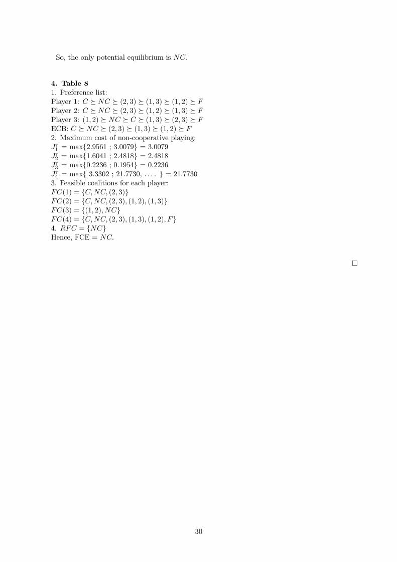
In Table 8 we assume that the inflation rates of countries 1 and 2 have an even stronger effect, thanin Table 6, on the inflation rate of country 3. This also changes the equilibrium outcome, as similarly,there is no profitable coalition; hence, the non-co-operative regime is the only equilibrium (CNE =SNE = FCE = NC - see the Appendix for a detailed description of the algorithm). Just recallthat with ς31 = ς32 = 0.2 in Table 6 full co-operation constituted the Pareto-superior equilibriumof the game. The full coalition cannot be sustained since country 3 has an incentive to deviate.The other players would prefer full co-operation but they suffer much higher welfare losses undernon-co-operation.
Table 8 — Country-specific shock with a high inflation importerParameters as in Table 5 except for ς31 = ς32 = 0.6
Figure 5 describes the adjustments of control and outcome variables in the non-co-operativeregime, such adjustments have clear similarities to Figures 3 and 4.
17
Figure 5 — Adjustments in the non-co-operative regime
0 20 40 60 80 100-0.5
-0.3
-0.1
0.1
0.3
0.5f
0 20 40 60 80 100-0.5
-0.3
-0.1
0.1
0.3
0.5f2
0 20 40 60 80 100-0.5
-0.3
-0.1
0.1
0.3
0.5f3
0 20 40 60 80 100-0.5
-0.3
-0.1
0.1
0.3
0.5iE
0 20 40 60 80 100-0.5
-0.3
-0.1
0.1
0.3
0.5y
y1y2y3
10 20 30 40 50 60 70 80 90 1000
0.2
0.4
0.6
0.8
1p
(a) Controls (b) Output gaps, prices
Concluding this section we can state that in a structural asymmetric setting the optimal policiesand the optimal outcomes become more complex. The magnitude of fiscal and inflation spilloversis crucial in determining the coalitional equilibrium (or equilibria) of the game. In general, theasymmetries reduce the gains from co-operation so that in many cases the full coalition cannot besupported without a transfer system (side-payments), which seems not to be very realistic in theEMU context.
4.4 SGP stringency and ECB priorities
In the context of our model we can also investigate the effects of two major policy institutions of theEU: (i) the SGP and (ii) the management of the monetary policy by the ECB. The SGP impliesthe accomplishment of fiscal targets by the BEPGs. In our model the effects of the SGP stringencycan be studied by considering different weights associated with the domestic fiscal deficit (χi fori ∈ {1, 2, 3}). The effects of more restrictive thresholds imposed by different BEPGs are representedin Table 9. To enable comparisons with the benchmark model as found in Table 1, the numericalsimulations in this section were based on the matrix of reduced form coefficients L(1).
18
Table 9 — SGP alternative thresholds (χi = 5, 10, 15 for i ∈ {1, 2, 3})31χi common shock [1,1,1]’ country-specific shock [1,0,-1]’
NC C F (1,2) (1,3) (2,3) NC C F (1,2) (1,3) (2,3)5 0.053 0.030 0.180 0.100 0.100 0.054 15.476 12.794 12.794 17.390 12.794 13.410
In the common shock case, losses of fiscal policymakers are decreasing in the thresholds except forthe initial equilibrium regime (C) that remains unchanged, regardless the increase in χi. Referringto the benchmark model analysis this result is easy to interpret. For χi = 5 the full coalition (C)is the single equilibrium (CNE =SNE =FCE = C), as it enables to internalise negative externalitiesof fiscal policies and it is the sole profitable coalition. However, increasing SGP stringency makesco-operation relatively less necessary, as excessive fiscal policies are independently limited by eachplayer. Already for χi = 10 non-co-operation (NC) is the equilibrium of the game (although, this isdue to the ECB’s deviation from full co-operation).
It can be expected, that for even higher values of χi, in as well the non-cooperative case, and thefull and partial fiscal coalitions cases, the losses of fiscal players will converge further to those of thefull co-operative case. This happens because, in the optimal co-operative strategies, fiscal players usemoderate fiscal expansions (see Figure 2).
In contrast to the common shock case, the fiscal policymakers’ optimal losses increase in thecountry-specific shock (p0 = [1, 0,−1]0) in all equilibria (C, F and (1, 3)) with increasing fiscalstringency32. This is obvious, since SGP stringency makes the fiscal response to the asymmetricshock more limited. Therefore, in contrast to a common shock, excessive fiscal stringency in the formof the SGP is not desirable in the case of an asymmetric shock. However, one needs to keep in mindthat the assumption of the symmetry of the countries is crucial in our analysis. The reason is theperfect off-setting of fiscal policies of both countries that experience exactly opposite shocks. In thepresence of asymmetries between countries this conclusion might no longer hold33.
To summarise, the above analysis shows that the increase of fiscal stringency is not desirable incase of a country-specific shock. However, in the case of a common shock, the negative (rule-based)co-ordination can diminish losses.
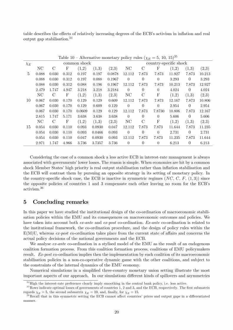
Consequences of different ECB’s interest rate preferences are investigated in Table 10. The tabletests the effects of different degrees of smoothing in the interest-rate management. Therefore, the
31Rows indicate optimal losses of governments for countries 1, 2 and 3, and the ECB, respectively. The first submatrixregards χi = 5, the second submatrix χi = 10, and, finally χi = 15, for i ∈ {1, 2, 3}.32Except for the ECB and country 2 whose losses equal 0.33For example, when the structural asymmetric case of Table 5 is considered, increased fiscal stringency in the
situation of a specific shock diminishes losses of all the players in the non-co-operative regime and increases losses forfiscal co-operation. For other regimes results are mixed.
19
table describes the effects of relatively increasing degrees of the ECB’s activism in inflation and realoutput gap stabilisation.34
Considering the case of a common shock a less active ECB in interest-rate management is alwaysassociated with governments’ lower losses. The reason is simple. When economies are hit by a commonshock Member States’ high priority is real output stabilisation rather than inflation stabilisation andthe ECB will contrast them by pursuing an opposite strategy in its setting of monetary policy. Inthe country-specific shock case, the ECB is inactive in symmetric regimes (NC, C, F , (1, 3)) sincethe opposite policies of countries 1 and 3 compensate each other leaving no room for the ECB’sactivism.36
5 Concluding remarks
In this paper we have studied the institutional design of the co-ordination of macroeconomic stabili-sation policies within the EMU and its consequences on macroeconomic outcomes and policies. Wehave taken into account both ex-ante and ex-post co-ordination. Ex-ante co-ordination is related tothe institutional framework, the co-ordination procedure, and the design of policy rules within theE(M)U, whereas ex-post co-ordination takes place from the current state of affairs and concerns theactual policy decisions of the national governments and the ECB.
We analyse ex-ante co-ordination in a stylised model of the EMU as the result of an endogenouscoalition formation process. From this coalition formation process, coalitions of EMU policymakersresult. Ex-post co-ordination implies then the implementation by each coalition of its macroeconomicstabilisation policies in a non-co-operative dynamic game with the other coalitions, and subject tothe constraints of the internal dynamics of the EMU economy.
Numerical simulations in a simplified three-country monetary union setting illustrate the mostimportant aspects of our approach. In our simulations different kinds of spillovers and asymmetries34High the interest-rate preference clearly imply smoothing in the central bank policy, i.e. less active.35Rows indicate optimal losses of governments of countries 1, 2 and 3, and the ECB, respectively. The first submatrix
regards χE = 5, the second submatrix χE = 10, and, finally, for χE = 15.36Recall that in this symmetric setting the ECB cannot affect countries’ prices and output gaps in a differentiated
manner.
20
have been considered since fiscal policy co-ordination is strongly connected with the externalities(fiscal spillovers) and asymmetries that are present in the economy. From the simulations somegeneral and robust conclusions can be drawn when several symmetries (but not all) are assumed.
In the case of a common shock, fiscal co-ordination is counterproductive but full policy co-ordination is desirable. By contrast, in case of a country-specific (asymmetric) shock, fiscal co-ordination is desirable and full policy co-ordination is not associated with any extra gain in thepolicymakers’ welfare. Our results add new features to the debate between Buti and Sapir (1998) andBeetsma et al. (2001) on the effects of co-ordination in the presence of shocks. Fiscal co-ordinationis deficient in the case of a common shock (as suggested by Beetsma et al. (2001)). Nevertheless, inthis situation the co-ordination among all policymakers improves the performance. The reason forthis is that full co-operation reduces the tensions between the ECB and the governments in pursuingdifferent priorities, and therefore, it reduces the costs of contrasted policies. On the contrary, fiscalco-operation increases such tensions since it increases the clash among the institutions that pursuedifferent priorities.
When asymmetric shocks are considered, fiscal co-ordination improves the performance by inter-nalising the traditional negative fiscal externalities (as sustained by Beetsma et al. (2001)) and fullpolicy co-ordination doesn’t produce further gains in the policymakers’ welfare since, in this case,there are no further externalities associated with the separate management of the fiscal and monetarypolicies.
SGP stringency and compliance with BEPGs are significant factors influencing the outcome ofthe game. In the case of a common shock, they can ensure lower losses in the situation, when fullco-ordination is not likely to emerge (e.g. because of exogenous political reasons). On the otherhand, increased fiscal stringency is counter-productive in the case of asymmetric shocks. However,this result is obtained in the setting of perfectly symmetric countries. In such a setting changesin the ECB’s policy rules prove that in the case of a common shock, full co-operation is needed tointernalise externalities.
Our approach also shows that it is of crucial importance to consider how coalitions are formed(ex-ante co-ordination). Following the recent literature, different coalition formation mechanisms canbe associated with different institutional settings where policymakers act. In fact, it can occur that,even if a co-operative solution assures for all the policymakers a lower loss than in the case of anon-co-operative solution, it does not emerge as an equilibrium of the game because of free-rider be-haviour which generally leads to non-co-operative solutions according to the CNE-mechanism (evenif co-operation is Pareto-superior to non-co-operation). In general, mechanisms where policymak-ers share more information (as the full co-operation (C), the SNE-mechanism (hierarchical), andthe FCE-mechanism (farsighted)), are more likely to support co-operative solutions avoiding free-riding behaviour than the traditional CNE-mechanism, which, however, seems to be the concept thatrepresents best the current EMU context.
The co-ordination of economic policies seems to be more difficult when the number and sizeof externalities become large. In this case, externalities are often associated with negative effectsirrespective of the kind of shocks or fiscal spillovers considered. The ex-post fiscal co-ordination resultsare strongly connected with the size and sign of externalities (fiscal spillovers) that are present in theeconomy. However, results under considerable asymmetries seem to be less robust, and, therefore,they have to be interpreted with caution.
A possible extension of the analysis concerns the introduction of outside-monetary-union coun-tries. This is a crucial issue as currently three EU Countries do not participate in the EMU and thegroup of EU accession countries in Central and Eastern Europe is entering on the 1st of May, 2004.It will also allow, among others, to study interactions between the EU and the USA economies, sincesignificant externalities may be present in that context.
Therefore, by solving the inflation equation, p(t) = (I − ς)−1 ζx(t), and plugging this result inthe output gap equation, we get: x(t) = −γιniE(t) + ηf(t) + γ (I − ς)−1 ζx(t) + δp(t) + ρx(t), fromwhich we obtain the reduced form for the real output gaps:
x(t) =³I − γ (I − ς)−1 ζ − ρ
´−1(−γιniE(t) + ηf(t) + δp(t))
and for the inflation rates:
p(t) = (I − ς)−1 ζ³I − γ (I − ς)−1 ζ − ρ
´−1(−γιniE(t) + ηf(t) + δp(t))
Rearranging: ·x(t)p(t)
¸= L
p(t)f(t)iE(t)
= · D E MA B N
¸ p(t)f(t)iE(t)
where:
D :=³I − γ (I − ς)−1 ζ − ρ
´−1δ
E :=³I − γ (I − ς)−1 ζ − ρ
´−1η
M := −³I − γ (I − ς)−1 ζ − ρ
´−1γιn
A := (I − ς)−1 ζ³I − γ (I − ς)−1 ζ − ρ
´−1δ
B := (I − ς)−1 ζ³I − γ (I − ς)−1 ζ − ρ
´−1η
N := − (I − ς)−1 ζ³I − γ (I − ς)−1 ζ − ρ
´−1γιn
22
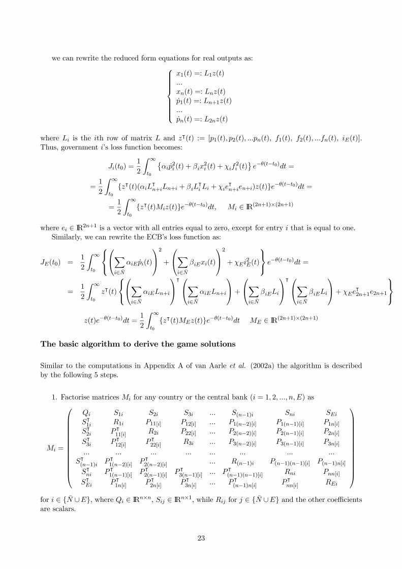
we can rewrite the reduced form equations for real outputs as:
where ei ∈ IR2n+1 is a vector with all entries equal to zero, except for entry i that is equal to one.Similarly, we can rewrite the ECB’s loss function as:
JE(t0) =1
2
Z ∞
t0
X
i∈NαiE pi(t)
2 +X
i∈NβiExi(t)
2 + χEi2E(t)
e−θ(t−t0)dt =
=1
2
Z ∞
t0
z|(t)
X
i∈NαiELn+i
|Xi∈N
αiELn+i
+X
i∈NβiELi
|Xi∈N
βiELi
+ χEe|2n+1e2n+1
z(t)e−θ(t−t0)dt =
1
2
Z ∞
t0
{z|(t)MEz(t)}e−θ(t−t0)dt ME ∈ IR(2n+1)×(2n+1)
The basic algorithm to derive the game solutions
Similar to the computations in Appendix A of van Aarle et al. (2002a) the algorithm is describedby the following 5 steps.
1. Factorise matrices Mi for any country or the central bank (i = 1, 2, ..., n, E) as
S|(n−1)i P |1(n−2)[i] P |2(n−2)[i] ... R(n−1)i P(n−1)(n−1)[i] P(n−1)n[i]S|ni P |1(n−1)[i] P |2(n−1)[i] P |3(n−1)[i] ... P |(n−1)(n−1)[i] Rni Pnn[i]S|Ei P |1n[i] P |2n[i] P |3n[i] ... P |(n−1)n[i] P |nn[i] REi
for i ∈ {N ∪E}, where Qi ∈ IRn×n, Sij ∈ IRn×1, while Rij for j ∈ {N ∪E} and the other coefficientsare scalars.
where Bi is the ith column of matrix B. Then, we can define the following matrix:
H : = H1 +H2G−1H3
4. After computing the eigenstructure of H, take n positive eigenvalues and the correspondingeigenvectors vi to write the following expression:37
XY1Y2...YnYE
:=¡v1 v2 ... vn
¢:= V ∈ IRn(n+2)×n
from which we can derive the optimal controls:f1(t)f2(t)...
fn(t)iE(t)
= −G−1
S|11 +B|1K1
S|22 +B|2K2
...S|nn +B|nKn
S|EE +M|EKn+1
p =: Fp
37 If matrix H has more than n positive eigenvalues multiple equilibria arise, whereas if this matrix has less than npositive eigenvalues no equilibrium exists (for more details see Engwerda (1998)).
24
where Ki := YiX−1 for i ∈ {N ∪E}.
5. Rewrite the policymakers’ cost functions38 and the dynamics of the model as Ji(t) = 12
R∞0 p|
·(I, F |)Mi
µIF
dt and p(t) = (A+ (BN) F ) p(t) =: ACLp(t), respectively. The problem is then solved by considering:
Ji = p|0Xip0
where Xi solves the following Lyapunov equation (for i ∈ {N ∪E}):
A|CLXi +XiACL +1
2(I, F |)Mi
µIF
¶= 0
Co-operative solutions are achieved by using the same algorithm but considering joint lossesminimisation39.
Two algorithms for calculating coalitional equilibria
Two algorithms are presented which give two different ways how coalitions might be formed. Thefirst one is based on Bloch’s (1996) ideas and describes a sequential process how coalitions might beformed. The second is based on the idea of farsightedness and describes which coalitions can be ruledout in this situation. It does not determine what will happen but what possibly can happen. Thesequential coalition formation process (computing the SNE) and the farsighted process (computingthe FCE) should mimic the various cases.
The sequential coalition formation process
1. In order to determine the order of moves in the sequential game of coalition formation, fix arule of order for the players.
2. The first player starts the game according to the rule of order by considering the questionwhether it is rational for her to propose a coalition. To that end she considers the worstpossible outcome that can occur if she does not form a coalition, i.e.40:
Jr1 := max({1},{.})J1(.).
If Jr1 is smaller than the cost she infers by forming whatever coalition, player 1 will propose nocoalition and leaves the game. That is, the game continues with step 2. with player 1 playingnon-cooperatively and player 2 starting the game.If there is at least one coalition form where the cost of player 1 is lower than Jr1 we assume
41
that player 1 will propose a coalition according to the following rules:
38For reasons of convenience, we assume that t0 = 0 and θ is equal to zero. Assuming θ different from zero, themodel could easily be solved following the procedure used in this paper after a simple transformation of variables, i.e.transforming x(t) into e−
12 θtx(t) and substituting A by A− 1
2θI where I ∈ IRn×n is a diagonal matrix with ones on the
main diagonal (see Engwerda et al. (1999), p.263, for further details).39For more details see e.g.: van Aarle et al. (2002b) or Engwerda et al. (2002, Appendix B).40Notation: ({1} {.}) denotes the case in which player 1 plays non-coperatively, whereas other players may form any
coalitions (but may also play non-co-operatively).41Note that we assume here that player 1 is risk averse, i.e. it might happen that e.g. in the non-cooperative case her
cost is lower than the minimal cost she can incur by forming any coalition. However, since she is not able to enforcethe non-cooperative solution, we choose to select this definition of rationality.
25
i) Select that coalition where her cost is as small as possible.
ii) If there is more than one coalition satisfying i), choose that coalition containing the mostimportant players.
iii) If there is more than one coalition satisfying ii), select that coalition which contains thehighest number of players.
Rules ii) and iii) say that e.g. the coalition {1,2,3} is preferred above the coalitions {1,2}and {1,2,4}.Next proceed with step 3.
3. Verify whether all players in the coalition agree on this coalition according to the rule of order.That is: player i agrees on this coalition if her cost in this coalition is smaller or equal thanboth the cost she incurs by joining any other feasible coalition and the worst possible outcomeif she does not join any feasible coalition. The set of feasible coalitions is determined by thehistory of the game. That is, the set of feasible coalitions, FC, contains only those coalitionswhich are still realisable given the history of the game. More formally, verify whether:
Ji(coalition) ≤ min{ min({i,..},{..})∈FC
Ji(.), max({i},{..})∈FC
Ji(.)}.
holds for all players in the foreseen coalition.
4. If all players agree on the coalition, the coalition is formed and the players leave the game. Thecoalition process repeats with the remaining players from step 2. on.If not all players agree, the first player who disagrees may come up with a coalition proposalif she did not have this opportunity for this set of feasible coalitions before. In that case thecoalition process repeats from step 2. on. Otherwise, a cycle has occurred, and the coalitionformation process would repeat itself ad infinitum. We assume that in that case all playersthat are still involved in the formation process all play non-co-operatively.
Examples:
1. Table 41. Order: 1,2,3,ECB2. Player 1 may propose:Jr1 = max{5.1464 ; 3.9647} = 5.1464Player 1 proposes the fiscal coalition F as:FC(1) = 3.3142 = min{3.4654; 3.3142; 4.2673; 11.5036} < Jr1 = 0.5.1464
3. Reaction of other players to the proposal of the Player 1:Player 2 rejects as:FC(2) = 14.5786 > min{min{14.0739, 18.2389, 18.2389}, max{22.0439; 17.5804}}
= min {14.0739; 22.0439} = 14.07394. Player 2 may propose:Jr2 = max{22.0439; 17.5804} = 22.0439;Player 2 proposes the full coalition F as:F (2) = 14.0739 < min{18.2389} < Jr1 = 22.0439;
5. Reaction of other players to the proposal of the Player 2:Player 1 accepts as:C(1) = 3.4654 < min{min{4.2673; 11.5036} , max{5.1464, 3.9647}}
3. Table 71. Choose as the rule of order, 1,2,3,ECB.2. Player 1 may propose.Jr1 = max({1},{..}) J1(.) = max{0.4788, 0.3933} = 0.4788.0.269 = min({1,..},{..}) J1(.) < Jr1 . So, player 1 chooses the full coalition C.3. Player 2 accepts.Player 3 does not accept as 0.5124 > min{min{0.5841, 0.4395, 0.5822},max{0.4776, 0.5137}}= 0.4395.2. player 3 may propose.Jr3 = max{0.4776, 0.4395} = 0.4776.Jr3 < min{0.5124, 0.5841, 0.5137, 0.5822}. So, player 3 prefers to play non-co-operatively.2. player 1 may propose.Since player 3 plays non-cooperatively, the set of feasible coalitions contains only (1,2).As 0.4788 < 0.6254 player 1 chooses a non-co-operative mode of play too.2. player 2 may propose.Since both player 1 and player 2 play non-co-operatively, the set of feasible coalitions is NC.So, player 3 is forced to play non-co-operatively too as well as the ECB.Hence, NC results.
4. Table 81) The selected order: 1,2,3,ECB2) Player 1 may propose:Jr1 = max {2.9561; 3.0079} = 3.0079Player 1 finds that coalition C = 0.2587 = min{0.2587; 17.0234; 8.2460; 4.2768}Since C < Jr1 Player 1 proposes C.
= min{2.1750; 2.4814} = 2.17504) Player 3:C(3) = 0.5870 > min = {min{4.7338; 0.9831; 2.1569}, max{0.2236; 0.1954}}
= min{0.9831; 0.2236} = 0.2236 = NC(3)Players 3 rejects.5) Player 3 proposes:Jr3 = max{0.2236; 0.1954} = 0.2236;NC(3) = 0.2236 < min{4.7338; 0.9831; 2.1569} = 0.9831Player 3 decides to play non-co-operatively.6) Player 1 may propose:The only feasible coalition for P1 is now only (1,2).Since NC(1) < (1,2)(1) Player 1 decides to play non-cooperatively.7) Since Players 1 and 3 play non-co-operatively there are no other possible coalitions.Hence, SNE = NC.
¤
The farsighted coalition process
1. Make a preference list for each of the individual players, i.e. for each player determine whichcoalition yields the lowest cost, the one-but lowest cost etc.
2. Determine for each player i the minimum cost it can enforce by playing non-cooperatively, i.e.determine for each i
Jri := max({i},{..})
Ji(.).
3. Determine for each player i all coalitions for which Ji(.) ≤ Jri . Denote this set of feasiblecoalitions for each player i by FC(i).
4. Determine all coalitions which are in the intersection of all sets of feasible coalitions. Call thisset the Rational Feasible Coalitions set (RFC).
5. Drop within the set RFC those coalitions which are Pareto dominated by another coalition.That is, if e.g. both coalitions F and C belong to RFC but C is preferred by every playerabove F , the coalition F is dropped from the set RFC.
6. Look for coalitions within this set that satisfy some additional properties as internal and ex-ternal stability, or exogenous factors that support certain equilibria.
Examples:
1. Table 41. Preference list:Player 1: F º C º (2, 3) º (1, 2) º NC º (1, 3)Player 2: C º F º (1, 3) º (1, 2) = (2, 3) º NCPlayer 3: F º C º (1, 2) º (2, 3) º NC º (1, 3)ECB: C º NC º F º (1, 2) = (2, 3) º (1, 3)2. Maximum cost of non-cooperative playing:Jr1 = max{5.1464 ; 3.9647} = 5.1464;
28
Jr2 = max{22.0439; 17.5804} = 22.0439;Jr3= max{5.1464 ; 3.9647} = 5.1464;Jr4 = max{ 0.2155, 0.3398; . . . } = 1.9266.3. FC for each player:FC(1) = {F,C, (2, 3), (1, 2)}FC(2) = {C,F, (1, 3), (1, 2), (2, 3)}FC(3) = {F,C, (2, 3), (1, 2)}FC(4) = {C,NC, (2, 3), (1, 3), (1, 2), F}5. RFC = {C,F}6. The final coalitional outcome - C or F - depends on other factors that are included into the
algorithm - e.g. exogenous political factors as the existence of a transfer system. Since, the combinedloss of all the players is lower in the full coalition than in the fiscal coalition, the C-regime would bechosen more likely in that case.
Hence, FCE = C,F.2. Table 6
1. Preference list:Player 1: C º (2, 3) º NC º (1, 3) º (1, 2) º FPlayer 2: C º NC º (1, 3) º (1, 2) º F º (2, 3)Player 3: C º (1, 3) º (1, 2) º NC º (2, 3) º FECB: C º NC º (2, 3) º (1, 3) º (1, 2) º F2. Maximum cost of non-cooperative playing:Jr1 = max{0.8495 ; 0.5601} = 0.8495Jr2 = max{0.2324 ; 0.2611} = 0.2324Jr3= max{0.9284 ; 0.9259} = 0.9284Jr4 = max{ 1.3575; 4.7440; . . . } = 4.74403. Feasible coalitions for each player:FC(1) = {C, (2, 3), NC}FC(2) = {C,NC}FC(3) = {C, (1, 3), (1, 2), NC}FC(4) = {C,NC, (2, 3), (1, 3), (1, 2), F}5. RFC = {C,F, }6.NC is Pareto-dominated by C as all C(i) Â NC(i)Hence, FCE = C.
3. Table 71. The preference list is as follows:1: C º (1, 3) º (2, 3) º NC º F º (1, 2)2: C º (1, 3) º NC º F º (1, 2) º (2, 3)3: (1, 2) º NC º C º (1, 3) º (2, 3) º FECB: C º (2, 3) º NC º (1, 3) º (1, 2) º F2. Jr1 = max{0.4788, 0.3933} = 0.4788.Jr2 = max{0.0627, 0.0513} = 0.0627.Jr3 = max{0.4776, 0.4395} = 0.4776.Jr4 = max{1.1638, 1.4047, 1.3364, 1.1756, 1.1383} = 1.4047
Aarle, B. van, J. Engwerda and J. Plasmans (2002a), ”Monetary and fiscal policy interaction in theEMU: A dynamic game approach”, Annals of Operations Research, vol. 109, pp. 229-264.
Aarle, B. van, G. Di Bartolomeo, J. Engwerda and J. Plasmans (2002b), ”Coalitions and dynamicinteractions between fiscal and monetary authorities in the EMU”, Ifo Studien, vol. 48, No. 2,pp. 207-229.
Acocella,. N. and G. Di Bartolomeo (2001), “Wage and public expenditure setting in a monetaryunion”, Working Paper No. 42., Department of Public Economics, University of Rome ‘LaSapienza’.
Agell, J., L. Calmfors and G. Jonsson (1996), “Fiscal policy when monetary policy is tied to themast”, European Economic Review, vol. 40: 1413-1440.
d’Aspremont, C.A., A. Jacquemin, J.J. Gabszewicz and J. Weymark (1983) “On the stability ofcollusive price leadership”, Canadian Journal of Economics, vol. 16, pp. 17-25.
Beetsma, R.M.W.J. and Bovenberg A.L. (1998), “Monetary union without fiscal coordination maydiscipline policymakers?”, Journal of International Economics, vol. 45, pp. 239-258.
Beetsma, R.M.W.J., X. Debrun and F. Klaassen (2001), “Is fiscal policy coordination in EMU desider-able?”, CESIfo Working Paper No. 599, Center for Economic Studies and Ifo Institute for Eco-nomic Research, Munich.
Bloch, F. (1996), “Sequential formation of coalitions in games with externalities and fixed payoffdivision”, Games and Economic Behavior, vol. 14, pp. 90-123.
Buti, M. and A. Sapir (Eds.) (1998), Economic Policy in EMU: A Study by the European CommissionServices, Oxford University Press, Oxford.
CESifo (2002), Report on the European Economy 2002, Center for Economic Studies and Ifo Institutefor Economic Research, Munich.
Chwe, M.S. (1994), “Farsighted coalitional stability”, Journal of Economic Theory, vol. 54, pp. 299-325.
Clarida, R., J. Galí and M. Gertler (1999), ”The Science of Monetary Policy: A New KeynesianPerspective”, Journal of Economic Literature, vol. 37, pp. 1661-1707.
Debrun, X. (2000) “Fiscal rules in a monetary union: a short run analysis”, Open Economies Review,vol. 11, pp. 323-358.
Di Bartolomeo, G., J.C. Engwerda and J.E.J. Plasmans (2002a), “Stabilization policies in a monetaryunion: Two-stage games of endogenous fiscal coalition formation”, Working Paper.
Di Bartolomeo, G., J.C. Engwerda, J.E.J. Plasmans and B. van Aarle (2002b), “Staying togetheror breaking apart: Policy-makers’ endogenous coalitions formation in the European Economicand Monetary Union”, Working Paper No. 13, Faculty of Applied Economics UFSIA-RUCA,University of Antwerp and CESifo Working Paper No. 748, Center for Economic Studies and IfoInstitute for Economic Research, Munich.
Di Bartolomeo, B. Merlevede, J. Plasmans and B. van Aarle (2003), ”Monetary Policy regimes in theNew Keynesian Framework: Results for Accession Countries”, mimeo, University of Antwerp.
31
DiNardo, J. and M.P. Moore (1999), “The Phillips Curve is Back? Using Panel Data to Analyze theRelationship Between Unemployment and Inflation in an Open Economy”, National Bureau ofEconomic Research Working Paper No. 7328.
ECB (1999), “The stability-oriented monetary policy in the Eurosystem”, Monthly Bulletin (Janu-ary), Frankfurt, ECB.
Ecchia, G. and M. Mariotti (1998), “Coalition formation in international environmental agreementsand the role of institutions”, European Economic Review, vol. 42, pp. 573-582.
Engwerda, J. (1998), “Computational aspects of the open-loop Nash equilibrium in linear quadraticgames”, Journal of Economic Dynamics and Control, vol. 22, pp. 1487-1506.
Engwerda, J., B. van Aarle and J. Plasmans (1999), “The (in)finite horizon open-loop Nash LQgame: An application to the EMU”, Annals of Operations Research, vol. 88, pp. 251-273.
Engwerda, J., B. van Aarle and J. Plasmans (2002), “Cooperative and non-cooperative fiscal stabil-isation policies in the EMU”, Journal of Economic Dynamics and Control, vol. 26, pp. 451-481.
Favero, C., X. Freixas, T. Pesson and C. Wyplosz (2000), “One money many countries, monitoringthe European Central Bank 2”, London, Center for Economic Policy Research.
Issing, O. (1999), “The Eurosystem: transparent and accountable, or Willem in Euroland”, Journalof Common Market Studies, vol.. 37, pp. 503-521.
Jensen, H. (1996), “The advantage of international fiscal cooperation under alternative monetaryregimes”, European Journal of Political Economy, vol. 12, pp. 485-504.
Kehoe, T. (1988), “Policy coordination among benevolent governments may be undesirable”, Reviewof Economic Studies, vol. 56, pp. 289-296.
Mariotti, M. (1998), “A model of agreements in a strategic form games”, Journal of Economic Theory,vol. 73, pp. 128-139.
Monteforte, L. and S. Siviero, ”Aggreate vs. Disaggregate Euro-Area Maco-Modelling”, mimeo, Bankof Italy.
Monfort, A., J.P. Renne, R. Ruffer and G. Vitale (2002), ”Is Economic Activity in the G7 Synchro-nised? Common Schock vs. Spillovers Effects”, mimeo.
Levine, P. and A. Brociner (1994), “Fiscal policy coordination and EMU”, Journal of EconomicDynamics and Control, vol. 18, pp. 699-729.
Onorante, L. (2002), “The interaction of fiscal policies in the Euro area: how much pressure on theECB?“, Cambridge, Cambridge University Press, forthcoming.
Ray, D. and R. Vohra (1999). “A theory of endogenous coalition structures”, Games and EconomicBehavior, vol. 26, pp. 286-336.
Razin, A. and C.W. Yuen (2001), “The ‘New Keynesian’ Phillips curve: Closed economy vs. openeconomies”, National Bureau of Economic Research Working Paper No. 8313.
Rogoff, K. (1985), “Can international monetary cooperation be counterproductive?”, Journal ofInternational Economics, vol. 18, pp. 199-217.
Uhlig, H.(2002), “One money, but many fiscal policies in Europe: what are the consequences?”,CentER Discussion Paper No. 32.