Macroeconomic Theory IV: New Keynesian Economics

Gavin Cameron Lady Margaret Hall

Michaelmas Term 2004

new Keynesian theories• Real Business Cycle models suggests that booms and busts are

equilibrium responses to the constraints faced by optimising agents.

• In contrast, New Keynesian models suggest that business cycles occur because nominal wages and prices are slow to adjust to changes in aggregate demand. Incomplete nominal adjustment leads to the failure of the classical dichotomy (incomplete real adjustment will not suffice, q.v. efficiency wages).

• But why might nominal adjustment be incomplete?• Staggered Wages and Prices;• Small Menu Costs and Aggregate Demand Externalities;• Recessions as Coordination Failures;• Credit Channels.

staggered price models• Three popular models:

• Fischer 1977, Phelps & Taylor 1977;• Taylor 1979, 1980;• Caplin & Spulber 1987.

• In the first two, wages or prices are set by multiperiod contracts. In each period, the contracts governing some predetermined fraction of prices are renewed. Multiperiod contracts lead to gradual adjustment of the price level to nominal disturbance.

• Time dependent: Fischer model assumes prices are predetermined but not fixed (i.e. different prices can be set in each period). Taylor model assumes fixed prices throughout contract.

• State dependent: In the Caplin-Spulber, price changes are determined endogenously so that the fraction of prices that changes each period can vary.

staggered wage & price adjustment• Not everyone in the economy sets new wages and prices

every period. Instead, adjustment is staggered. Staggering makes the overall level of wages and prices adjust slowly even when individual wages and prices change frequently. In this case, aggregate demand policy can be stabilizing even when expectations are rational.

• In any period, half of prices are the ones set in the previous period and half are the ones set two periods ago.

• Thus the average price is (1)

• where pt1 is the price set for t by individuals who set prices

at t-1 and pt2 the price set for t by those who set prices at t-2.

1 21 ( )2t t t

p p p= +

an aggregate demand shock• Consider an aggregate demand shift that becomes

known after the first prices are set. One might expect that since half of prices are already set and the other half are free to adjust, half of the shift is passed into prices and half into output.

• This is not true though, since firms that are able to change their prices also take into account the fact that other firms will not be able to change their prices.

the adjustment of real prices• Consider how a firm changes its real price in response to a change

in aggregate real output:

(2)

• A lower value of φ corresponds to greater real rigidity since firms are unwilling to adjust their real prices when aggregate output changes. Real rigidity alone does not cause monetary disturbances to have real effects: if prices can adjust freely, money is neutral regardless of the value of φ. But real rigidity magnifies the effect of nominal rigidity: a low value of φ implies that price-setters are unwilling to allow variations in their relative prices. As a result, the price-setters that are free to adjust their prices do not allow their prices to differ greatly from those already set.

p*

it t tp c yφ− = +

implications for prices and output• It turns out that prices and output in the Fischer model evolve

according to:

(3)

(4)

• As in the Lucas model, unanticipated aggregate demand shifts have real effects: this is shown by the mt-Et-1mt term. Because price-setters do not know mt when they set prices, these shocks are passed one-for-one into output.

2 1 2( )

1t t t t t t tp E m E m E mφ

φ− − −= + −

+

1 2 1

1 ( ) ( )1t t t t t t t t

y E m E m m E mφ − − −

= − + −+

the effect of shocks• However, aggregate demand shifts that become

anticipated after prices are first set also affect output. The proportion (1/1+φ) of a change in m that becomes known between t-2 and t-1 is passed into output, the remainder goes into prices.

• Note that if φ=1, then ½ of a shock goes into output, as our intuition suggests, but if φ>1 then price-setters make large changes and the aggregate real effects of changes are small.

Caplin & Spulber, 1987• The Fischer and Taylor models assume that the timing of price

changes is determined by the passage of time. However, since all contracts are, in principle, renegotiable, perhaps it is better to think of the timing as being endogenous.

• Caplin-Spulber model a situation with an Ss rule: whenever a price-setter adjusts her price, she sets it so that the difference between the actual and the optimal price is some target level S. The nominal price is then fixed until the optimal level has changed such that the trigger level s is reached. This is optimal when inflation is steady.

• In contrast to the Fischer model, money is neutral in the Caplin-Spulber model since the number of price-setters changing their prices at any one time is an increasing function of the money supply growth rate.

• Caplin-Spulber shows that state-dependent price changes are important and that even when prices are fixed for most price-setters, the actions of other price-setters can be offsetting. So far, we haven’t considered whether there is a cost to price adjustment generally.

menu costs• Prices may not adjust immediately when economic

conditions change, because there may be costs to price adjustment.

• When a firm cuts prices, it slightly lowers the average price level and thereby raises real money balances and aggregate demand. Therefore, each firm’s price decision has an aggregate-demand externality.

• The firm ignores this externality when making pricing decisions and therefore may not change prices frequently enough.

a simple menu cost model• Economy begins in

equilibrium at point A. A fall in AD with other prices unchanged shifts the demand curve inwards. If firm doesn’t change price, output falls to B, if it does then output is C. The area D represents the profits from the price reduction.

• The firm is harmed by the failure of other firms to cut their prices in the fall of the fall in AD. As a result it may find that the gain from reducing its price is small even if the shift in its demand curve is large.

P

Q

MC

D

P1

Q0 Q1

A

C

B

D’

MR

MR’

D

the effects of menu costs• A fall in aggregate demand with other prices unchanged

reduces aggregate output and thus shifts in the demand curve that the firm faces. At any given price, demand for the firm’s product is lower.

• If the firm does not cut its price, output is determined by the existing price (point B). At this level of output, MR>MC so thefirm has an incentive to lower its price and raise output. For the firm to be willing to hold its price fixed, the additional profits must be small.

• The firm is harmed by the failure of other firms to cut prices. As a result, the firm may find that the gain from a price cut issmall even if the fall in demand is large.

the profit function• Consider a firm deciding whether

to change its price in the face of a fall in aggregate demand with other prices fixed. The figure shows the firm’s profits as a function of its price. The fall in aggregate output affects this function in two ways. First, since the demand for the firm’s good falls, the profit function shifts down. Second, the profit-maximising price is less than before.

• The firm’s incentive to change its price is therefore given by the distance AB in the figure. This distance depends on two factors: the difference between the old and new profit-maximizing prices and the curvature of the profit function.

π

P

AB

C D

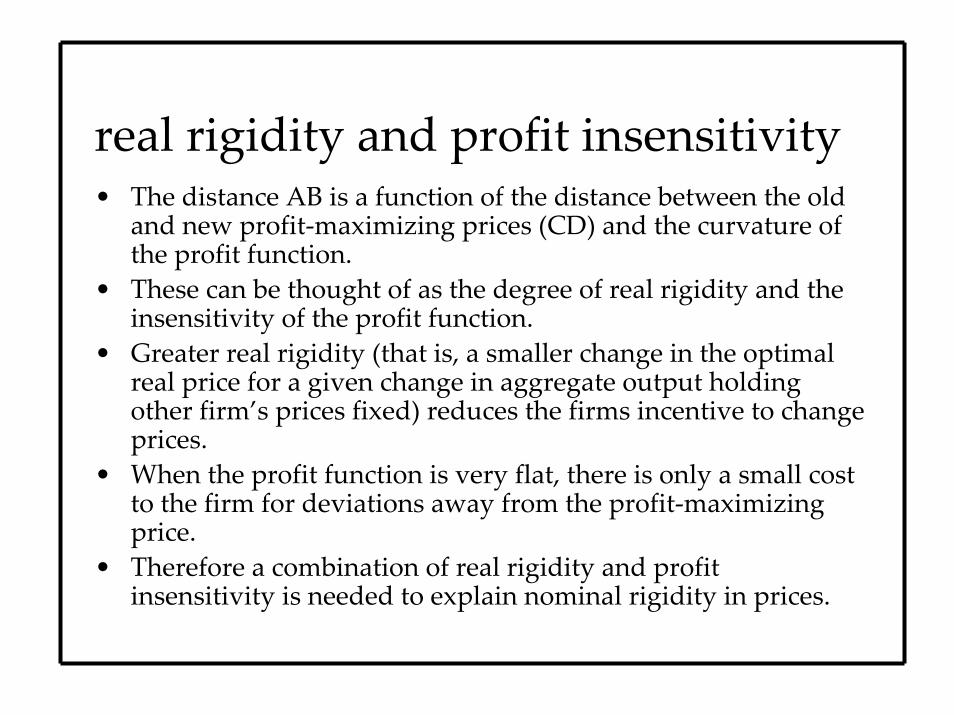
real rigidity and profit insensitivity• The distance AB is a function of the distance between the old

and new profit-maximizing prices (CD) and the curvature of the profit function.

• These can be thought of as the degree of real rigidity and the insensitivity of the profit function.

• Greater real rigidity (that is, a smaller change in the optimal real price for a given change in aggregate output holding other firm’s prices fixed) reduces the firms incentive to changeprices.

• When the profit function is very flat, there is only a small cost to the firm for deviations away from the profit-maximizing price.

• Therefore a combination of real rigidity and profit insensitivity is needed to explain nominal rigidity in prices.

the sources of real rigidity• Marginal Cost

• A smaller fall in marginal cost as a result of a fall in aggregate output, the smaller the incentive to cut prices since it implies a smaller decline in the profit-maximizing price (real rigidity).

• A flatter marginal cost curve implies that profits are less sensitive to movements away from profit-maximizing output (profit insensitivity and real rigidity).

• Marginal Revenue• The larger the fall in marginal revenue when aggregate

output falls, the smaller the gap between marginal revenue and marginal cost at the firm’s initial price and so there is less incentive to adjust prices (real rigidity).

recessions as coordination failure• Consider a firm which, after a fall in aggregate

demand, must decide whether to cut output.• The firm’s profits depend upon the decision of the

other firms. In general, the firm’s output is likely to be increasing in the other firm’s output.

• Consider the simplest case where two firms simultaneously choose their output levels for the production of a complementary good: a stag hunt game.

simple stag hunt game

High Output

Low Output

High Output Low Output

5 5

x’ 30

x

3

0• This game has two pure

strategy Nash equilibria. But which one gets selected?

• To calculate the risk dominant equilibrium, calculate the products of the deviation payoffs, i.e. (5-x)(5-x) and (3-0)(3-0). The larger of these is risk dominant.

• X>2 bad equilibrium is risk-dominant

• X<2 good equilibrium is risk-dominant

Cooper and John, 1988• The economy consists of multiple identical agents, who wish

to choose the value of some variable, say, output.• The firm wants to maximize Ui=v(yi,y) when firm I chooses

output yi and everyone else chooses y.• We denote yi*(y) as the choice of the firm given the choices of

all other firms.• Equilibrium occurs where yi*(y)=y, that is, no firm will change

its choice given the choices of other firms.• If this reaction function is linear, we are get a unique

equilibrium in the coordination game. If it is non-linear, we get multiple Pareto-ranked equilibria.

a unique equilibriumyi*

y

yi*(y)E

45º

multiple equilibria

yi*

y

yi*(y)

C

A

B

45º

With multiple equilibria, fundamentals do not fully determine outcomes. If agents expect the economy to be at C, it ends up there.

multiple equilibria and real rigidity• Real rigidity occurs when, in response to an increase in the

price level and a decline in aggregate output, a firm only wants to change its relative price slightly.

• This corresponds to a reaction function with a slope of just less than 1: when aggregate output falls, the firms wants its sales to decline almost as much as the others.

• The existence of multiple equilibria suggests that over some range, declines in aggregate output cause the firm to want to raise its price and thus reduce sales relative to others. Thus the reaction function has a slope of more than 1 over some range.

• Therefore multiple equilibria require strong real rigidity over some range of output.

the credit channel• In traditional models, asset prices do not matter for the real

economy.• But in markets with informational asymmetries, firms prefer

to finance investments from internal rather than external funds due to the external finance premium.

• Why might investment be sensitive to the source of finance?• The Cash Flow Channel

• A positive (negative) monetary shock raises (reduces) current output and cash flow and hence reduces (increases) the proportion of investment that must be externally financed. Thislowers (raises) the cost of capital and raises (reduces) investment

• The Asset Price Collateral Channel• A positive (negative) monetary shock raises (reduces) asset prices

and hence raises (reduces) the value of collateral. The rise (fall) in the value of collateral reduces (raises) the external financepremium and hence raises (reduces) investment.

summary• It is a combination of real and nominal rigidity that

leads to incomplete nominal adjustment.• New Keynesian models can seem vague and

flexible, so this leads to skepticism.• Central prediction is that nominal wages and prices

do not adjust immediately and that independent monetary disturbances should affect real activity.

• There is lots of evidence that price and wage adjustment is sticky, but sizes and timing of price changes do not entirely fit the predictions of any NK model.