92
Macroeconomics I E_EBE1_MACEC Prof. dr. Eric Bartelsman 26 & 27 februari 2018

Macroeconomics IE_EBE1_MACEC
Prof. dr. Eric Bartelsman26 & 27 februari 2018

Overview
• Introduction to Business Cycles– Aggregate Demand and Aggregate Supply
• Aggregate Demand Curve– Keynesian Cross– Money Demand and Money Supply– IS-LM model
• Aggregate Supply• Stabilization Policy

The model of aggregate demand and supply
• the paradigm most mainstream economists and policymakers use to think about economic fluctuations and policies to stabilize the economy
• shows how the price level and aggregate output are determined
• shows how the economy’s behavior is different in the short run and long run

Income = Expenditures (slide from Economic Challenges, week 3 Macro)
Tesla’s, Y
Arbeidsuren, L
P*Y
w*L

Aggregate demand
• The aggregate demand curve shows the relationship between the price level and the quantity of output demanded.
• For this chapter’s intro to the AD/AS model, we use a simple theory of aggregate demand based on the quantity theory of money.
• Chapters 11-13 develop the theory of aggregate demand in more detail.

The Quantity Equation as Aggregate Demand
• From Chapter 4, recall the quantity equationM V = P Y
• For given values of M and V, this equation implies an inverse relationship between P and Y :

The downward-sloping AD curve
An increase in the price level causes a fall in real money balances (M/P),causing a decrease in the demand for goods & services.
Y
P
AD
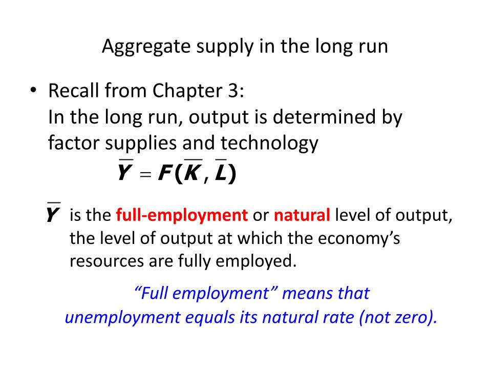
Aggregate supply in the long run
• Recall from Chapter 3: In the long run, output is determined by factor supplies and technology
,= ( )Y F K Lis the full-employment or natural level of output, the level of output at which the economy’s resources are fully employed.
Y
“Full employment” means that unemployment equals its natural rate (not zero).

The long-run aggregate supply curve
Y
P LRASdoes not
depend on P, so LRAS is vertical.
Y
( )= ,YF K L

Long-run effects of an increase in M
Y
P
AD1
LRAS
Y
An increase in M shifts AD to the right.
P1
P2In the long run, this raises the price level…
…but leaves output the same.
AD2

Aggregate supply in the short run
• Many prices are sticky in the short run. • For now (and through Chap. 13), we assume – all prices are stuck at a predetermined level in the
short run.– firms are willing to sell as much at that price level
as their customers are willing to buy. • Therefore, the short-run aggregate supply
(SRAS) curve is horizontal:

The short-run aggregate supply curve
Y
P
P SRAS
The SRAS curve is horizontal:The price level is fixed at a predetermined level, and firms sell as much as buyers demand.

Short-run effects of an increase in M
Y
P
AD1
In the short run when prices are sticky,…
…causes output to rise.
P SRAS
Y2Y1
AD2
…an increase in aggregate demand…

From the short run to the long run
Over time, prices gradually become “unstuck.” When they do, will they rise or fall?
Y Y>Y Y<Y Y=
rise
fall
remain constant
In the short-run equilibrium, if
then over time, P will…
The adjustment of prices is what moves the economy to its long-run equilibrium.

The SR & LR effects of DM > 0
Y
P
AD1
LRAS
Y
P SRASP2
Y2
A = initial equilibrium
AB
CB = new short-run
eq’m after Fed increases M
C = long-run equilibrium
AD2

Monetary Policy in a Recession
Y
P
AD1
LRAS
Y
P SRAS
Pn
Y1
A = initial recession
A
B
C
B = long-run equilibrium without monetary policy
C =eq’m after CB increases M
AD2

Overview
• Introduction to Business Cycles– Aggregate Demand and Aggregate Supply
• Aggregate Demand Curve– Keynesian Cross– Money Demand and Money Supply– IS-LM model
• Aggregate Supply• Stabilization Policy

The Keynesian Cross• A simple closed economy model in which income is
determined by expenditure. (due to J.M. Keynes)
• Notation: I = planned investmentE = C + I + G = planned expenditureY = real GDP = actual expenditure
• Difference between actual & planned expenditure = unplanned inventory investment

Elements of the Keynesian Cross( )C C Y T= -
I I=
,G G T T= =
( )E C Y T I G= - + +
=Y E
consumption function:
for now, plannedinvestment is exogenous:
planned expenditure:
equilibrium condition:
govt policy variables:
actual expenditure = planned expenditure

Graphing planned expenditure
income, output, Y
Eplanned
expenditureE =C +I +G
MPC1

Graphing the equilibrium condition
income, output, Y
Eplannedexpenditure
E =Y
45º

The equilibrium value of income
income, output, Y
Eplanned
expenditureE =Y
E =C +I +G
Equilibrium income

An increase in government purchases
Y
EE =Y
E =C +I +G1
E1 = Y1
E =C +I +G2
E2 = Y2DY
At Y1, there is now an unplanned drop in inventory…
…so firms increase output, and income rises toward a new equilibrium.
DG

Solving for DYY C I G= + +
Y C I GD = D + D + D
MPC= ´ D + DY GC G= D + D
(1 MPC)- ´D = DY G1
1 MPCæ ö
D = ´ Dç ÷-è øY G
equilibrium condition
in changes
because I exogenous
because DC =MPCDY
Collect terms with DY on the left side of the equals sign:
Solve for DY :

The government purchases multiplier
Example: If MPC = 0.8, then
Definition: the increase in income resulting from a $1 increase in G.In this model, the govt purchases multiplier equals 1
1 MPCD
=D -YG
1 51 0.8
D= =
D -YG
An increase in G causes income to increase 5 times
as much!

Why the multiplier is greater than 1
• Initially, the increase in G causes an equal increase in Y:DY = DG.
• But Y ÞCÞ further YÞ further CÞ further Y
• So the final impact on income is much bigger than the initial DG.

The IS curvedef: a graph of all combinations of r and Y that result in goods market equilibriumi.e. actual expenditure (output)
= planned expenditure
The equation for the IS curve is:

Y2Y1
Y2Y1
Deriving the IS curve
¯r Þ I
Y
E
r
Y
E =C +I (r1 )+GE =C +I (r2 )+G
r1
r2
E =Y
IS
DIÞ E
Þ Y

Why the IS curve is negatively sloped
• A fall in the interest rate motivates firms to increase investment spending, which drives up total planned spending (E).
• To restore equilibrium in the goods market, output (a.k.a. actual expenditure, Y) must increase.

The IS curve and the loanable funds model
S, I
r
I (r )r1
r2
r
YY1
r1
r2
(a) The L.F. model (b) The IS curve
Y2
S1S2
IS

Fiscal Policy and the IS curve
• We can use the IS-LM model to see how fiscal policy (G and T) affects aggregate demand and output.
• Let’s start by using the Keynesian cross to see how fiscal policy shifts the IS curve…

Y2Y1
Y2Y1
Shifting the IS curve: DG
At any value of r, GÞE ÞY
Y
E
r
Y
E =C +I (r1 )+G1
E =C +I (r1 )+G2
r1
E =Y
IS1
The horizontal distance of the IS shift equals
IS2
…so the IS curve shifts to the right.
11 MPC
D = D-
Y G DY

The Theory of Liquidity Preference
• Due to John Maynard Keynes.• A simple theory in which the interest rate
is determined by money supply and money demand.

Money supply
The supply of real money balances is fixed:
The picture can't be displayed.
M/Preal money
balances
rinterest
rate
The picture can't be displayed.
M P

Money demand
Demand forreal money balances:
M/Preal money
balances
rinterest
rate( )sM P
M P
L (r )

Equilibrium
The interest rate adjusts to equate the supply and demand for money:
M/Preal money
balances
rinterest
rate( )sM P
M P
( )M P L r= L (r )r1

How the CB raises the interest rate
To increase r, CB reduces M
M/Preal money
balances
rinterest
rate
1MP
L (r )r1
r2
2MP

The LM curve
Now let’s put Y back into the money demand function:
The LM curve is a graph of all combinations of r and Y that equate the supply and demand for real money balances.The equation for the LM curve is:

Deriving the LM curve
M/P
r
1MP
L (r ,Y1 )r1
r2
r
YY1
r1L (r ,Y2 )
r2
Y2
LM
(a) The market for real money balances (b) The LM curve

Why the LM curve is upward sloping
• An increase in income raises money demand. • Since the supply of real balances is fixed, there
is now excess demand in the money market at the initial interest rate.
• The interest rate must rise to restore equilibrium in the money market.

How DM shifts the LM curve
M/P
r
1MP
L (r ,Y1 )r1
r2
r
YY1
r1
r2
LM1
(a) The market for real money balances (b) The LM curve
2MP
LM2

The short-run equilibrium
The short-run equilibrium is the combination of r and Y that simultaneously satisfies the equilibrium conditions in the goods & money markets:
Y
r
IS
LM
Equilibriuminterestrate
Equilibriumlevel ofincome

The Big PictureKeynesianCross
Theory of Liquidity Preference
IScurve
LMcurve
IS-LMmodel
Agg. demand
curve
Agg. supplycurve
Model of Agg.
Demand and Agg. Supply
Explanation of short-run fluctuations

Chapter Summary1. Keynesian cross
– basic model of income determination– takes fiscal policy & investment as exogenous– fiscal policy has a multiplier effect on income.
2. IS curve– comes from Keynesian cross when planned investment
depends negatively on interest rate– shows all combinations of r and Y
that equate planned expenditure with actual expenditure on goods & services
slide 44

Chapter Summary3. Theory of Liquidity Preference
– basic model of interest rate determination– takes money supply & price level as exogenous– an increase in the money supply lowers the interest rate
4. LM curve– comes from liquidity preference theory when
money demand depends positively on income– shows all combinations of r and Y that equate demand
for real money balances with supply
slide 45

Chapter Summary5. IS-LM model
– Intersection of IS and LM curves shows the unique point (Y, r ) that satisfies equilibrium in both the goods and money markets.
slide 46

Macroeconomics IE_EBE1_MACEC
Prof. dr. Eric Bartelsman27 februari 2018

The intersection determines the unique combination of Y and rthat satisfies equilibrium in both markets.
The LM curve represents money market equilibrium.
Equilibrium in the IS-LM model
The IS curve represents equilibrium in the goods market.
ISY
rLM
r1
Y1

Exercise: Shifting the IS curve
• Use the diagram of the Keynesian cross or loanable funds model to show how an increase in taxes shifts the IS curve.

Instant Poll
• An increase in taxes:– A. Shifts the IS curve to the left, by less than the
amount of a similar decrease in G– B. Shifts the IS curve to the right, by less than the
amount of a similar decrease in G– C. Shifts the IS curve to the left, by more than the
amount of a similar decrease in G– D. Shifts the IS curve to the right, by more than
the amount of a similar decrease in G

An increase in taxes
Y
EE =Y
E =C2 +I +G
E2 = Y2
E =C1 +I +G
E1 = Y1DY
At Y1, there is now an unplanned inventory buildup……so firms reduce
output, and income falls toward a new equilibrium
DC = -MPC DT
Initially, the tax increase reduces consumption, and therefore E:

Solving for DYY C I GD = D + D + D
( )MPC= ´ D - DY T
C= D
(1 MPC) MPC- ´D = - ´ DY T
eq’m condition in changes
I and G exogenous
Solving for DY :
MPC1 MPCæ ö-
D = ´ Dç ÷-è øY TFinal result:

The tax multiplierdef: the change in income resulting from a $1 increase in T :
MPC1 MPC
D -=
D -YT
0.8 0.8 41 0.8 0.2
D - -= = = -
D -YT
If MPC = 0.8, then the tax multiplier equals

IS11.
…Now a tax cut
Y
rLM
r1
Y1
IS2
Y2
r2
Consumers save (1-MPC) of the tax cut, so the initial boost in spending is smaller for DT than for an equal DG… and the IS curve shifts by
MPC1 MPC
T-D
-1.
2.
2.…so the effects on rand Y are smaller for DTthan for an equal DG.
2.

Policy analysis with the IS-LM model
We can use the IS-LM model to analyze the effects of• fiscal policy: G and/or T• monetary policy: M IS
Y
rLM
r1
Y1

causing output & income to rise.
IS1
An increase in government purchases
1. IS curve shifts right
Y
rLM
r1
Y1
1by 1 MPC
GD-
IS2
Y2
r2
1.2. This raises money demand, causing the interest rate to rise…
2.
3. …which reduces investment, so the final increase in Y
1is smaller than 1 MPC
GD-
3.

Exercise: Shifting the LM curve
• Suppose a wave of credit card fraud causes consumers to use cash more frequently in transactions.
• Use the liquidity preference model to show how these events shift the LM curve.

Instant Poll
• Using IS-LM, the increase in preference for cash results in a new equilibrium with:– A. higher r, higher Y– B. higher r, lower Y– C. lower r, higher Y– D. lower r, lower Y

2. …causing the interest rate to fall
IS
Monetary policy: An increase in M
1. DM > 0 shifts the LM curve down(or to the right)
Y
r LM1
r1
Y1 Y2
r2
LM2
3. …which increases investment, causing output & income to rise.

Interaction between monetary & fiscal policy
• Model: Monetary & fiscal policy variables (M, G, and T) are exogenous.
• Real world: Monetary policymakers may adjust Min response to changes in fiscal policy, or vice versa.
• Such interaction may alter the impact of the original policy change.

The Central Bank response to DG > 0
• Suppose Gov’t increases G.• Possible CB responses:
1. hold M constant2. hold r constant3. hold Y constant
• In each case, the effects of the DGare different:

If Gov’t raises G, the IS curve shifts right.
IS1
Response 1: Hold M constant
Y
rLM1
r1
Y1
IS2
Y2
r2If CB holds M constant, then LM curve doesn’t shift.
Results:
2 1Y Y YD = -
2 1r r rD = -

If Gov’t raises G, the IS curve shifts right.
IS1
Response 2: Hold r constant
Y
rLM1
r1
Y1
IS2
Y2
r2To keep r constant, CB increases Mto shift LM curve right.
3 1Y Y YD = -
0rD =
LM2
Y3
Results:

IS1
Response 3: Hold Y constant
Y
rLM1
r1IS2
Y2
r2To keep Y constant, CB reduces Mto shift LM curve left.
0YD =
3 1r r rD = -
LM2
Results:
Y1
r3
If Gov’t raises G, the IS curve shifts right.

Estimates of fiscal policy multipliersfrom the US-DRI macroeconometric model
Assumption about monetary policy
Estimated value of DY/DG
Fed holds nominal interest rate constant
Fed holds money supply constant
1.93
0.60
Estimated value of DY/DT
-1.19
-0.26

Shocks in the IS-LM modelIS shocks: exogenous changes in the demand for goods & services.
Examples: – stock market boom or crash
Þ change in households’ wealthÞDC
– change in business or consumer confidence or expectations ÞDI and/or DC

Shocks in the IS-LM model
LM shocks: exogenous changes in the demand for money.
Examples:– Worry about safety of Banks increases demand
for money.– more ATMs or the Internet reduce money
demand.

EXERCISE:Analyze shocks with the IS-LM model
Use the IS-LM model to analyze the effects of1. a boom in the stock market that makes consumers
wealthier.2. after a bursting housing bubble, and fear of
banking crisis, people want more cash.
For each shock, a. use the IS-LM diagram to show the effects of the
shock on Y and r.b. determine what happens to C, I, and the
unemployment rate.

Instant Poll
• Using IS-LM, a boom in the stock market results in a new equilibrium with:– A. higher r, higher Y– B. higher r, lower Y– C. lower r, higher Y– D. lower r, lower Y

Instant Poll
• In the new equilibrium following the boom in the stock market:– A. C is higher, I is lower– B. C is higher, I is higher– C. C is lower, I is lower– D. C is lower, I is higher

EXERCISE:Analyze shocks with the IS-LM model
Use the IS-LM model to analyze the effects of1. a boom in the stock market that makes consumers
wealthier.2. after a bursting housing bubble, and fear of
banking crisis, people want more cash.
For each shock, a. use the IS-LM diagram to show the effects of the
shock on Y and r.b. determine what happens to C, I, and the
unemployment rate.

IS-LM and aggregate demand• So far, we’ve been using the IS-LM model
to analyze the short run, when the price level is assumed fixed.
• However, a change in P would shift LM and therefore affect Y.
• The aggregate demand curve(introduced in Chap. 10) captures this relationship between P and Y.

Y1Y2
Deriving the AD curve
Y
r
Y
P
IS
LM(P1)LM(P2)
AD
P1
P2
Y2 Y1
r2r1
Intuition for slope of AD curve:
P Þ¯(M/P)
Þ LM shifts left
Þr
ޯIޯY
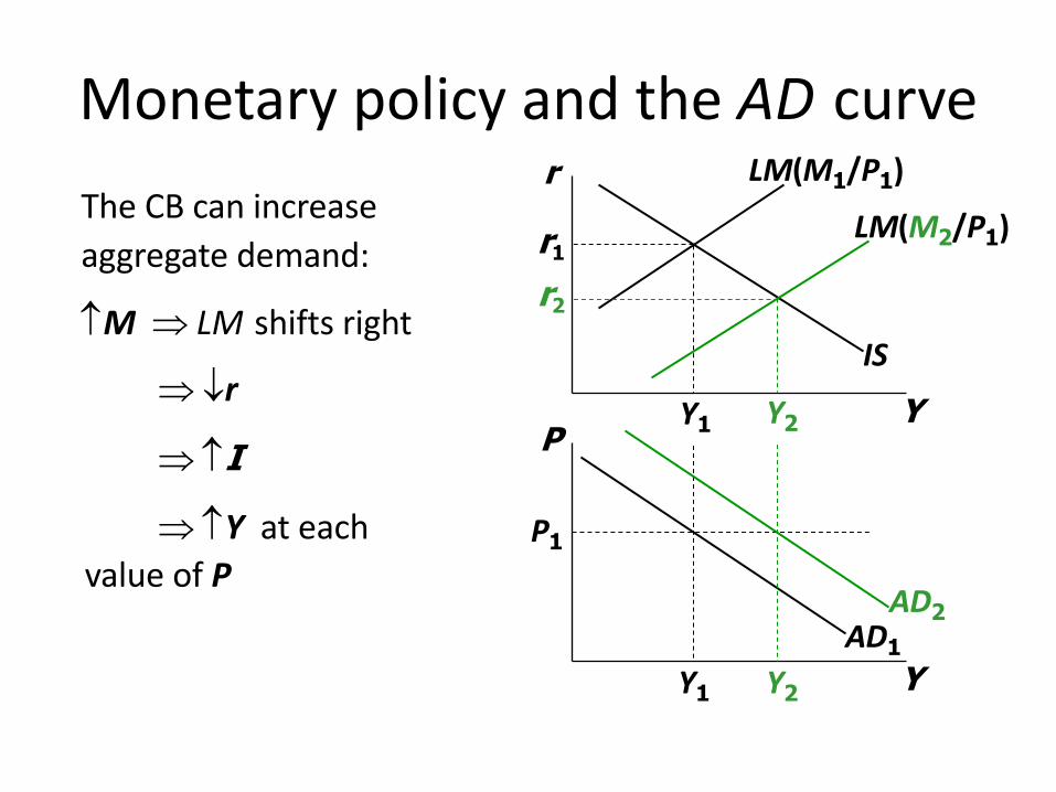
Monetary policy and the AD curve
Y
P
IS
LM(M2/P1)LM(M1/P1)
AD1
P1
Y1
Y1
Y2
Y2
r1r2
The CB can increase aggregate demand:
M Þ LM shifts right
AD2
Y
r
Þ¯r
ÞIÞY at each
value of P

Y2
Y2
r2
Y1
Y1
r1
Fiscal policy and the AD curve
Y
r
Y
P
IS1
LM
AD1
P1
Expansionary fiscal policy (G and/or ¯T) increases agg. demand:
¯T ÞC
Þ IS shifts right
ÞY at each value of P
AD2
IS2

IS-LM and AD-AS in the short run & long run
Recall from Chapter 10: The force that moves the economy from the short run to the long run is the gradual adjustment of prices.
Y Y>Y Y<Y Y=
rise
fall
remain constant
In the short-run equilibrium, if
then over time, the price level will

The SR and LR effects of an IS shock
A negative IS shock shifts IS and AD left, causing Y to fall.
Y
r
Y
P LRAS
Y
LRAS
Y
IS1
SRAS1P1
LM(P1)
IS2
AD2AD1

The SR and LR effects of an IS shock
Y
r
Y
P LRAS
Y
LRAS
Y
IS1
SRAS1P1
LM(P1)
IS2
AD2AD1
In the new short-run equilibrium, Y Y<

The SR and LR effects of an IS shock
Y
r
Y
P LRAS
Y
LRAS
Y
IS1
SRAS1P1
LM(P1)
IS2
AD2AD1
In the new short-run equilibrium, Y Y<
Over time, P gradually falls, which causes•SRAS to move down.•M/P to increase, which
causes LMto move down.

AD2
The SR and LR effects of an IS shock
Y
r
Y
P LRAS
Y
LRAS
Y
IS1
SRAS1P1
LM(P1)
IS2
AD1
SRAS2P2
LM(P2)
Over time, P gradually falls, which causes•SRAS to move down.•M/P to increase, which
causes LMto move down.

AD2
SRAS2P2
LM(P2)
The SR and LR effects of an IS shock
Y
r
Y
P LRAS
Y
LRAS
Y
IS1
SRAS1P1
LM(P1)
IS2
AD1
This process continues until economy reaches a long-run equilibrium with
Y Y=

EXERCISE:Analyze SR & LR effects of DM
a. Draw the IS-LM and AD-ASdiagrams as shown here.
b. Suppose the CB increases M.Show the short-run effects on your graphs.
c. Show what happens in the transition from the short run to the long run.
d. How do the new long-run equilibrium values of the endogenous variables compare to their initial values?
Y
r
Y
P LRAS
Y
LRAS
Y
IS
SRAS1P1
LM(M1/P1)
AD1

The Great Depression
Unemployment (right scale)
Real GNP(left scale)
120
140
160
180
200
220
240
1929 1931 1933 1935 1937 1939
billi
ons o
f 195
8 do
llars
0
5
10
15
20
25
30
perc
ent o
f lab
or fo
rce

THE SPENDING HYPOTHESIS:
Shocks to the IS curve
• asserts that the Depression was largely due to
an exogenous fall in the demand for goods &
services – a leftward shift of the IS curve.
• evidence:
output and interest rates both fell, which is
what a leftward IS shift would cause.

THE SPENDING HYPOTHESIS:
Reasons for the IS shift• Stock market crash Þ exogenous ¯C– Oct-Dec 1929: S&P 500 fell 17%– Oct 1929-Dec 1933: S&P 500 fell 71%
• Drop in investment– “correction” after overbuilding in the 1920s– widespread bank failures made it harder to obtain
financing for investment• Contractionary fiscal policy– Politicians raised tax rates and cut spending to combat
increasing deficits.

THE MONEY HYPOTHESIS:
A shock to the LM curve• asserts that the Depression was largely due to
huge fall in the money supply.• evidence: M1 fell 25% during 1929-33.
• But, two problems with this hypothesis:– P fell even more, so M/P actually rose slightly
during 1929-31. – nominal interest rates fell, which is the opposite of
what a leftward LM shift would cause.

THE MONEY HYPOTHESIS AGAIN:
The effects of falling prices
• asserts that the severity of the Depression was
due to a huge deflation:
P fell 25% during 1929-33.
• This deflation was probably caused by the fall
in M, so perhaps money played an important
role after all.
• In what ways does a deflation affect the
economy?

THE MONEY HYPOTHESIS AGAIN:
The effects of falling prices• The stabilizing effects of deflation:• ¯P Þ(M/P) Þ LM shifts right ÞY• Pigou effect:
¯P Þ(M/P) Þ consumers’ wealth Þ C Þ IS shifts right ÞY

THE MONEY HYPOTHESIS AGAIN:
The effects of falling prices
• The destabilizing effects of expected deflation:
¯pe
Þ r for each value of iÞ I ¯ because I = I(r )
Þ planned expenditure & agg. demand ¯Þ income & output ¯

THE MONEY HYPOTHESIS AGAIN:
The effects of falling prices• The destabilizing effects of unexpected deflation:
debt-deflation theory¯P (if unexpected)
Þ transfers purchasing power from borrowers to lenders
Þ borrowers spend less, lenders spend more
Þ if borrowers’ propensity to spend is larger than lenders’, then aggregate spending falls, the IS curve shifts left, and Y falls

Chapter Summary1. IS-LM model
– a theory of aggregate demand– exogenous: M, G, T,
P exogenous in short run, Y in long run – endogenous: r,
Y endogenous in short run, P in long run – IS curve: goods market equilibrium– LM curve: money market equilibrium
slide 91

Chapter Summary2. AD curve– shows relation between P and the IS-LM model’s
equilibrium Y. – negative slope because P Þ¯(M/P ) Þr Þ¯I Þ¯Y
– expansionary fiscal policy shifts IS curve right, raises income, and shifts AD curve right.
– expansionary monetary policy shifts LM curve right, raises income, and shifts AD curve right.
– IS or LM shocks shift the AD curve.
slide 92


