33
Institute of Economic Theories - University of Miskolc Zoltán Bartha, PhD Associate Professor Macroeconomics Introduction to Economic Fluctuations Andrea S. Gubik, PhD Associate Professor
| Date post: | 02-Sep-2018 |
| Category: |
Documents |
| Upload: | vuongduong |
| View: | 216 times |
| Download: | 0 times |

Institute of Economic Theories - University of Miskolc
Zoltán Bartha, PhDAssociate Professor
Macroeconomics
Introduction to Economic Fluctuations
Andrea S. Gubik, PhDAssociate Professor

Business cycle: short-run fluctuations in output and employment
Recession: a period of falling output and rising unemployment
Expansion: a period of increasing output
Stagnation: a period of little or no growth in the economy
Growth in French Real GDP, 1980-2010
-3
-2
-1
0
1
2
3
4
5
1980
1982
1984
1986
1988
1990
1992
1994
1996
1998
2000
2002
2004
2006
2008
2010

French Unemployment (percent of total labour force) 1980-2010
The unemployment rate rises significantly during periods of recession. There is
a
negative (when one rises, the other
falls) relationship between unemployment and GDP.
6
7
8
9
10
11
12
1980
1982
1984
1986
1988
1990
1992
1994
1996
1998
2000
2002
2004
2006
2008
2010

Negative
relationship between the price level P and quantity of goods and services demanded Y.
Output (Y)
Pric
e le
vel
AD
As the price level decreases, we’d
move down along the AD curve.Any economic phenomena that causes changes in the value of C, I, G, NX
variables changes aggregate demand.
Aggregate demand (AD) is the relationship between the quantity of output demanded and the aggregate price level.
Pric
e le
vel
Output (Y)
AD'AD

Aggregate supply (AS) is the relationship between the quantity of goods and services
supplied and the price level.
The aggregate supply relationship depends on the time horizon.
The long run –
vertical AS curvePrices are flexibleIs called the natural level of output
-
at which
the economy’s
resources are fully employed, or more realistically, at which
unemployment
is at its natural rate.
PP
Y=F (K, L)YYYY
LRAS
AD
P
Y
P
AD
SRAS
The short run –
horizontal AS curve
Prices
are sticky and therefore short-run AS is horizontal

From the short run to the long run
PP
YY
LRASLRAS
YY
Y = F (K,L)Y = F (K,L)
ADAD
SRASSRAS
PP
YY
LRASLRAS
YY
ADAD
SRASSRAS
ADAD''
AABB
CC
The economy begins in long-run equilibrium at point A. Then, a reduction in aggregate demand, moves the economy from point A to point B, where
output is below its natural level. As prices fall, the economy recovers from
the recession, moving from point B to point C.

ShocksExogenous changes in aggregate supply or aggregate demand. supply shock: a
shock that affects aggregate supply.
demand shock a shock that affects aggregate demand.Stabilization PolicyPolicy
actions taken to reduce the severity of short-run economic fluctuations.
Stabilization
policy seeks to dampen the business cycle by keeping output and employment as close to their natural rate as possible.
Shocks to AD PP
YY
LRASLRAS
YY
ADAD
SRASSRAS
ADAD''AABB
CCThe economy begins in long-run equilibrium at point A. An increase
in aggregate demand, moves
the economy from point A to point B, where output is above
its natural level. As prices rise, output
gradually returns to its natural
rate, and the economy moves from point B to point C.

Shocks to AS
PP
YY
LRASLRAS
YY
ADAD
SRASSRASAA
BB SRASSRAS''
PP
YY
LRASLRAS
YY
ADAD
SRASSRASADAD''AA
BB SRASSRAS''
There is no way to adjust aggregate demand to maintain full employment and keep the price level sable.
a) to hold AD constantb) to expand AD to prevent a
reduction in output and employment
Institute of Economic Theories - University of Miskolc
Aggregate Demand I: Building the IS-LM Model

The model of aggregate demand (AD) can be split into two parts:
1. IS model of the “goods market”
“IS stands for Investment Saving, plots the relationship between the interest rate and the level of income
that arises in the market for goods and services. 2. LM model of the “money market.”
LM stands for Liquidity Money.”
plots the relationship between the interest rate and the level of income that arises in the money market.
Because the interest rate influences both investment and money demand, it is the variable that links the two parts of the IS-LM model.
The IS-LM is the leading interpretation of Keynes’ work. The IS-LM model takes the price level as given and shows what causes income to change. It shows what causes AD to shift. Income, Output, Y
Price level, P
SRAS
AD
Y* Y*'
AD'AD''
Y*''

The Keynesian cross shows how income Y is determined for given levels
of planned investment I and fiscal policy G and T. We can use this model to show how income changes when one of the exogenous variables change. Actual expenditure is the amount households, firms and the government spend on goods and services (GDP). Planned expenditure is the amount households, firms, and the Government
would like
to spend on goods and services. The economy is in equilibrium when: Actual Expenditure
= Planned Expenditure or Y = E
Expenditure, E
Income, output, Y
Actual expenditure, Y=E
Planned expenditure,E = C + I + G
Y2 Y1Y*
The goods market and the IS curve

Changes in government purchases Higher
government purchases result in higher planned expenditure,
for any
given level of income.
The increase in income Y exceeds the increase in government purchases
ΔG.
->fiscal policy has a multiplied effect on income.
Expenditure, E
Income, output, Y
Actual expenditure, Y=E
Planned expenditure,E = C + I + G
Y1Y*
ΔGA
B
Government-purchases multiplier: ΔY/ΔG = 1 / (1 – MPC)
Tax multiplier: ΔY/ΔT = - MPC / (1 - MPC)
Planned expenditure,E = C + I + G
Investment, I
(a)
E
Income, output, Y
Y = E
r
Income, output, Y
r
I(r) IS
(b)
(c)
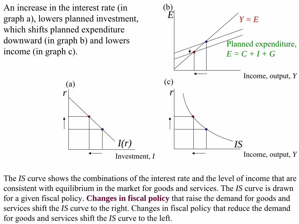
An increase in the interest rate (in graph a), lowers planned investment, which shifts planned
expenditure
downward (in
graph b) and lowers income (in graph c).
The IS curve shows the combinations of the interest rate and the level
of income that are consistent with equilibrium in the market for goods and services. The IS curve is drawn for a given fiscal policy. Changes in fiscal policy that raise the demand for goods and services shift the IS curve to the right. Changes in fiscal policy that reduce the demand for goods and services shift the IS curve to the left.

r
Supply of real money balances (M/P); both of these variables are taken to be exogenously given. This yields a vertical supply curve.Demand for real money balances, L. The theory of liquidity preference suggests that a higher interest rate lowers the quantity of real balances demanded, because
r
is the opportunity cost of holding money
(M/P)d = L (r,Y). The supply and demand for real money balances determine the interest rate. At the equilibrium interest rate, the quantity of money balances demanded equals the quantity supplied.
M/PM/P
Supply
Demand, L (r)
L(r) = M/P
r
M/PM/P
Supply
Demand, L (r,Y)
Supply'
Since the price level is fixed, a reduction in the money supply reduces
the supply of real
balances. The equilibrium interest rate rose.
The money market and the LM curve

r
M/PM/P
Supply
L (r,Y)'L (r,Y)
r1
r2
r
Y
LM
An increase in income raises money demand, which increases the
interest rate. The higher the level of income, the higher the interest rate.
Monetary policy and the LM curveLM curve is drawn for a given supply of real money balances. If real money balances change the LM curve shifts.
r
Y
LM(P0
)IS
r0
Y0
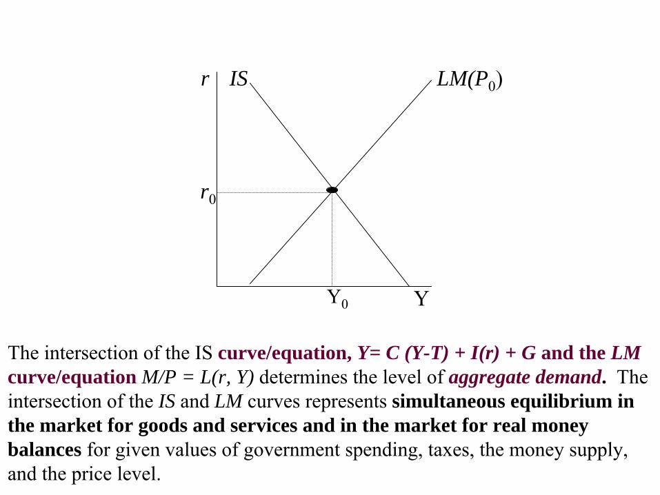
The intersection of the IS curve/equation, Y= C (Y-T) + I(r) + G and the LM curve/equation M/P = L(r, Y) determines the level of aggregate demand. The intersection of the
IS and LM curves represents simultaneous equilibrium in
the market for goods and services and in the market for real money balances for given values of government spending, taxes, the money supply, and the price level.

Institute of Economic Theories - University of Miskolc
Aggregate Demand II: Applying the IS-LM Model

How Fiscal Policy Shifts the IS Curve and Changes the Short-run Equilibrium
LMr
Y
IS
A
IS´
B
+ΔG will shift the IS curve to the right by ΔG/(1-
MPC).-ΔT will shift the IS curve to the right by ΔT × MPC/(1-
MPC).
The increase in Y in response to a fiscal expansion is smaller in the IS-LM model than in the Keynesian cross.
ISr
Y
LM
A LM′
B
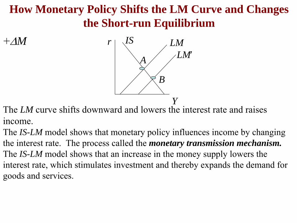
+ΔM
The LM curve shifts downward and lowers the interest rate and
raises income. The IS-LM model shows that monetary policy influences income by
changing
the interest rate. The
process
called the monetary transmission mechanism.The IS-LM model shows that an increase in the money supply lowers
the
interest rate, which stimulates investment and thereby expands the
demand for goods and services.
How Monetary Policy Shifts the LM Curve and Changes the Short-run Equilibrium

Suppose the government increases G.Possible central bank’s
responses:
•
1. hold M constant•
2. hold r constant
•
3. hold Y constantIn each case, the effects of the ΔG
are different.
r IS1
Y
LMIS2
IS1
Y
LM1IS2IS1
Y
IS2LM2 LM2
LM1rr
Interaction between monetary and fiscal policy

Shocks in the IS-LM model
IS shocks: exogenous changes in the demand for
goods & services. Examples:
•
stock market boom or crash–
a change in households’ wealth
–
ΔC•
change in business or consumer–
confidence or expectations
–
ΔI and/or ΔC
LM shocks: exogenous changes in the demand for
money.
Examples:•
a wave of credit card fraud increases demand for
money
•
more ATMs or the Internet reduce money demand

To derive AD, start at point A in the top graph. Now increase the price level from P1
to P2
. An increase in P lowers the value of real money balances, and Y, shifting LM leftward to point B. This raises the equilibrium interest rate and lowers the level of income.AD curve plots this inverse relationship between national income and price level.
rr
PP YY
YY
ISISLM(PLM(P11
))
AA
AAADAD
LM(PLM(P22
))
BB
BBP2P1
From IS-LM to AD
Events that shift the IS and the LM curves (for a given price level) cause AD curve to shift:An increase in M, G or a decrease in T raises Y
in the IS-LM model –
AD shifts
to the right.A decrease in M, G or an increase in T lowers Y in the IS-LM model –
AD
shifts to the left.

The IS-LM model in the short run and long run
We can also use IS-LM to describe the economy in the long run. K is the short run equilibrium –
the economy’s
income is less than its natural level. There is insufficient demand for goods and services to keep the economy producing at its potential –
P
decreases –
LM curve shifts to the right
-
C is the
long run
equilibrium.
The key difference between Keynesian assumption (K) and classical assumption (C) the time horizon:Classical assumption (Y=Y)best describes the long run, Keynesian assumption (P=P1
) best describes the short run.
LM (P1)
r
P Y
Y
IS
LM(P2)
ADP0
SRAS2K
K
C
C
LRASSRAS1
LRAS

Institute of Economic Theories - University of Miskolc
Aggregate Supply and the Short-run Tradeoff Between Inflation
and Unemployment

positive constant:an indicator of
how much
output responds
to unexpected changes in the
price level.
Y = Y + α(P‐EP) where α > 0P≠EPOutput
Actual price level
Natural rate of output
Expected price level
This equation states that output deviates from its natural level
when the
price level deviates from the expected price level. The parameter a
indicates how
much output responds to unexpected changes in the price
level, 1/ a
is the slope of the aggregate supply curve.
The Short-Run Aggregate Supply Equation
2
5
Some
market imperfection causes the output of the economy to deviate
from its natural level. As a result, the short-run aggregate supply curve is upward sloping, and shifts in the aggregate demand curve cause the level of output to deviate temporarily from its natural level.These temporary deviations represent the booms and busts of the business cycle.
Sticky-Wage Model
2
6
The Imperfect Information ModelThe model assumes that (1) markets clear - that is, all wages and prices are free to adjust to balance supply and demand. The short-run and long-run aggregate supply curves differ because of temporary misperceptions about prices. (2) Each supplier in the economy produces a single good and consumes many goods. Suppliers cannot observe all prices at all times. They monitor the prices of their own goods but not the prices of all goods they consume. Due to imperfect information, they sometimes confuse changes in the overall price level with changes in relative prices.This confusion influences decisions about how much to supply, and it leads to a positive relationship between the price level and output in the short run.
1. When the nominal wage is stuck, a rise in the price level lowers the real wage, making labour cheaper.2. The lower real wage induces firms to hire more labour.3. The additional labour produces more output.The aggregate supply curve slopes upward during the time when the nominal wage cannot adjust.

The Sticky-Price Model• Firms do not instantly adjust the prices they charge in
response to changes in demand. Sometimes prices are set by long-term contracts between firms and consumers.
• When firms expect a high price level, they expect high costs. Those firms that fix prices in advance set their prices high. These high prices cause the other firms to set high prices also. Hence, a high expected price level E leads to a high actual price level P.
• When output is high, the demand for goods is high. Firms with flexible prices set their prices high, which leads to a high price level.
• The firm’s desired price (P) depends on two macroeconomic variables: the overall level of prices (P) and the level of aggregate income (Y).
2
7

A: the economy is at full employment, the actual price level equals the expected price level.
B: Since P (the actual price level) is now greater than Pe (the expected price level) Y will rise above the natural rate, and we slide along the SRAS (Pe=P0
) curve to C .
The “long-run” will be defined when the expected price level equals the actual price level. So, as price level expectations adjust, EP⇒P2
, we’ll end up on a new short-run aggregate supply curve, SRAS (EP=P2
) at point C.
↑Y = Y + α (↑P-EP)
Y = Y + α (P-EP)
Y = Y + α (↑P-↑EP)
In terms of the SRAS equation, we can see that as EP catches up with P, that entire “expectations gap” disappears and we end up on the long run aggregate supply curve at full employment where Y = Y.
SRAS (EP=P2 )
CP2B
Y'
SRAS (EP=P0
)P
Output
AP0
LRAS*
YAD
AD'
P1
Short-run Aggregate Supply Curve in Action

The Phillips curve: represents
the trade-off between the inflation and unemployment in the short run.Inflation
rate
depends on three forces:
1) Expected inflation2) The deviation of unemployment from the natural rate, called cyclical unemployment3) Supply shocks
These three forces are expressed in the following equation:
π = Eπ − β(μ−μn) + εInflation b ×
Cyclical
unemploymentSupply shocks
Expected inflation
The Phillips Curve
2
9

1. Expected inflation: people form their expectations of inflation based on recently observed inflation = adaptive expectationsinflation has inertia, it keeps going until something acts to stop it
2. The deviation of unemployment from the natural rate, called cyclical unemployment = demand-pull inflation because high aggregate demand is responsible for this type of inflation
3. Supply shocks: inflation also rises and falls because of supply shocks. An adverse supply shock implies a positive value of n and causes inflation to rise = cost-push inflation

un
Inflation, π
Unemployment, u
Επ
+ ν
In the short run, inflation and unemployment
are negatively related. At any point in time, a
policymaker who controls aggregate demand
can choose a
combination of inflation and unemployment on this short-run Phillips curve.
The short‐run Trade‐off Between Inflation and Unemployment
The sacrifice ratio measures the
percentage of a year’s real GDP that must be foregone to reduce
inflation by 1 percentage point. A typical estimate of the ratio is 5.
Okun’s law: the negative relationship between unemployment and real GDP, according to which a decrease in unemployment of 1 percentage point is associated with additional growth in real GDP of approximately 2 per cent.

Rational Expectations and the Possibility of Painless DisinflationAdaptive expectations: People base their expectations of future inflation on recently observed inflation.Rational expectations: People base their expectations on all available information, including information about current and prospective future policies. Proponents of rational expectations believe that if policy makers are credibly committed to reducing inflation, rational people will understand the commitment and lower their expectations of inflation. Inflation can then come down without a rise in unemployment and fall in output.
32
Hysteresis and the Natural-Rate HypothesisOur entire discussion has been based on the natural rate hypothesis:Fluctuations in aggregate demand affect output and employment only in the short run. In the long run, the economy returns to the levels of output, employment, and unemployment described by the classical model.Recently, some economists have challenged the natural-rate hypothesis by suggesting that aggregate demand may affect output and employment even in the long run. They have pointed out a number of mechanisms through which recessions might leave permanent scars on the economy by altering the natural rate of unemployment. Hyteresis is the term used to describe the long-lasting influence of history on the natural rate.

Source: Mankiw, N.G. Macroeconomics. Worth Publishers, 2012
http://bcs.worthpublishers.com/mankiw8/default.asp


