Macroscopic constitutive equations of thermo ...

Philosophical MagazineVol. 91, No. 18, 21 June 2011, 2317–2342

Macroscopic constitutive equations of thermo-poroelasticity derived

using eigenstrain–eigenstress approaches

Alexander P. Suvorov and A.P.S. Selvadurai*

Department of Civil Engineering and Applied Mechanics, McGill University,QC, Canada H3A 2K6

(Received 15 June 2010; final version received 19 January 2011)

Macroscopic constitutive equations for thermoelastic processes in afluid-saturated porous medium are re-derived using the notion ofeigenstrain or, equivalently, eigenstress. The eigenstrain-stress approachis frequently used in micromechanics of solid multi-phase materials, such ascomposites. Simple derivations of the stress–strain constitutive relationsand the void occupancy relationship are presented for both fully saturatedand partially saturated porous media. Governing coupled equations for thedisplacement components and the fluid pressure are also obtained.

Keywords: fluid-saturated media; constitutive modeling; eigenstrain andeigenstress approaches; thermo-poroelastic models; unsaturated poroelasticmedia; homogenization techniques; effective poroelastic parameters

1. Introduction

The theory of poroelasticity can be regarded as an extension of the classical theory ofelasticity for a continuum, to account for a continuous pore structure in the mediumas well as the presence of fluids occupying the pore space. The classical theory in itscomplete form was proposed by Biot [1] and formed the basis for the theory ofconsolidation of a fluid-saturated soil with an elastic skeleton. Reviews of the subjectand recent developments in the area are given by Scheidegger [2], Paria [3], Rice andCleary [4], Selvadurai [5,6], Coussy [7], Verruijt [8] and Dormieux et al. [9], withapplications in the areas of bone mechanics [10,11], soft tissue mechanics andindentation problems [12,13], energy resources extraction and recovery [14] andgeoenvironmental applications related to geologic disposal of heat emitting nuclearfuel wastes [15–17].

In this paper, the equations governing the thermo-poroelastic response of a porousmedium, with either a saturated or an unsaturated pore space, are derived byconsidering approaches used in mechanics of solid heterogeneous materials. In theapplication of the theory of heterogeneous materials to thermo-mechanics ofporoelastic media, we consider two distinct scales: a microscale, over which thephases are alternated (or periodic), and the macroscale, which is comparable to theoverall dimensions of the region of interest. The fields within the heterogeneous body,

*Corresponding author. Email: [email protected]

ISSN 1478–6435 print/ISSN 1478–6443 online

� 2011 Taylor & Francis

DOI: 10.1080/14786435.2011.557402

http://www.informaworld.com

Dow

nloa

ded

by [

McG

ill U

nive

rsity

Lib

rary

] at

07:

16 2

7 N

ovem

ber

2015

such as temperature or stress, usually exhibit rapid fluctuations over the microscale.Homogenization procedures enable the smoothing of these fluctuations but also allowfor slow variations of the fields on a macroscale. The objective of the homogenizationprocedure is to determine the effective properties of the heterogeneous material, i.e.those properties that characterize the overall behavior or response of the materialregion to external influences, on a macroscale, and to formulate the relevant effectiveconstitutive relations (i.e. the relationships between the macroscopic fields). There arenumerous methods for determining the effective properties and examples are given invarious articles and texts [18–23]. To an observer, a heterogeneous body will appear asa homogeneous body that has variations of the fields only on the macroscale. Thehomogenized problem can be solved more conveniently since it invariably involvesa smaller number of degrees of freedom. The notion of effective properties ofa heterogeneous porous medium also finds useful application in the modeling ofpermeability [24].

This paper specifically deals with heterogeneous materials that have a solid butporous deformable skeleton through which the liquid phase can move; rocks andsoils are typical examples of such heterogeneous materials. Effective or macroscopicconstitutive relations for soils were first formulated by Biot [1]. This theory wassubsequently extended by several researchers to include the effects of compressibilityof both the fluid and solid phases [4]. Other extensions of the theory include thermaleffects, as given in several articles [16,25–27], where the constitutive relations for thethermo-poroelastic response of the medium, including the thermal expansion of boththe solid grains and the liquid, are taken into consideration. Rutqvist et al. [28]presented a comparative study of four theories for partially saturated geomaterialscontaining both liquid and air.

The objective of this paper is to link micromechanics (used primarily in studiesrelated to solid heterogeneous materials such as composites) with the macroscopictheory of poroelasticity and to re-derive the constitutive relations for the thermo-poroelastic behavior of a fluid-saturated medium. The approach we have chosen isdifferent from those presented in classical studies [4,16,27,29,30]. It relies on acombination of the definitions of eigenstresses or eigenstrains, as defined by Mura[31] and Dvorak et al. [32], and the general principles of micromechanics. A similarapproach was used by Chateau and Dormieux [33], who derived the equations ofporoelasticity by treating the fluid pressure as a prestress applied to the skeleton andusing Levin’s formula [34] to evaluate the contribution of this prestress to the overallstress. This methodology can be extended or modified if there are contributions tothe eigenstresses or eigenstrains resulting from processes other than thermal effects.Examples of these can include swelling, loss or gain of mass, eigenstrains associatedwith changes to the molecular structure of the phases or phase transformations andinelastic deformation.

The paper is organized as follows. Section 2 presents classical macroscopicconstitutive equations for a fully-saturated thermo-poroelastic continuum. Section 3gives, for completeness, a summary of the eigenstrain-stress approach. Thederivation of the constitutive equations for a partially saturated porous mediumbased on the eigenstrain-stress approach is presented in Section 4. Section 5 containsan example of a one-dimensional column of a porous linear elastic material subjectedto temperature change and surface loads at the boundary.

2318 A.P. Suvorov and A.P.S. Selvadurai

Dow

nloa

ded

by [

McG

ill U

nive

rsity

Lib

rary

] at

07:

16 2

7 N

ovem

ber

2015

2. Constitutive equations for thermo-poroelasticity

Consider a poroelastic body consisting of a porous fabric composed of an isotropiclinear elastic solid and pores which contain a non-viscous liquid. The solid phase(i.e. the material composing the porous medium) and liquid are assumed to becompressible. We first consider the case where the continuous pore space of themedium is fully saturated with the liquid. The porosity of the medium (the ratio ofthe volume of the pores to the total volume) is denoted by n. Assume that this porous

medium is subjected to heating (or cooling) and mechanical loads (Figure 1a). Theconstitutive relations that govern the behavior of such a porous medium at themacroscopic level will be presented in this section, without derivation.

Unlike composite materials, where the constitutive relation is written in terms ofthe elastic properties of the separate phases, the constitutive relationship forporoelastic materials is expressed in terms of the elastic constants of the drainedfabric (i.e. in the absence of any interaction between the pore fluids and the porousskeleton). Definition: under drained conditions, the fluid is allowed to flow in and outof the soil, but the fluid pressure remains independent of time [4]. For example, fullydrained conditions can prevail when the fluid pressure dissipates with time andeventually reaches zero. The effective mechanical properties and effective thermalexpansion coefficient of such a ‘‘drained geomaterial’’ will be equivalent to those ofthe soil skeleton with empty pores (note, however, that even when pressure is zero,

the liquid is present in the pore space since the soil is assumed to remain fullysaturated).

For a fully saturated thermoelastic geomaterial (under general, not necessarilydrained conditions), the macroscopic thermo-poroelastic relation is given by Riceand Cleary [4] and Savvidou and Booker [26]:

�ij ¼ 2GD"ij þ KD �2GD

3

� �"V�ij � 3KD�sT�ij � 1�

KD

Ks

� �p�ij, ð1Þ

Figure 1. Fully saturated porous medium subjected to tractions ti on the external boundaryand temperature change T. By applying the eigen-fields to the drained soil (b), we can simulatethe behavior of the porous medium under general, not necessarily drained conditions,as shown in (a).

Philosophical Magazine 2319

Dow

nloa

ded

by [

McG

ill U

nive

rsity

Lib

rary

] at

07:

16 2

7 N

ovem

ber

2015

where �ij is the total stress tensor; "ij is the strain tensor; "V ¼ "kk is the volumetric

strain; p is the fluid pressure; KD, GD are the bulk and shear moduli, respectively, of

the geomaterial under drained conditions; Ks is the bulk modulus of the solid phase;

�s is the coefficient of linear thermal expansion of the solid phase and T is the

temperature change. All field quantities (stresses, strains, pressure and temperature)

in (1) are, in general, functions of coordinates x ð¼ x1, x2, x3Þ and time.The last term in (1) represents the contribution of the fluid pressure to the total

stress. The multiplier in front of the pressure is referred to as the Biot parameter:

� ¼ 1�KD

Ks: ð2Þ

The second constitutive relation is sometimes referred to as the void occupancy

equation. The initial mass of fluid in the pore space is denoted by mf, and the change

in the mass of fluid is denoted by Dmf. Then, the void occupancy equation can be

expressed as [4]

nDmf

mf� � "V þ

�

Ku � KDp

� �þ n3�fTþ ð�� nÞ3�sT ¼ 0, ð3Þ

where Ku is the bulk modulus of the geomaterial under undrained conditions; �s, �fare coefficients of thermal expansion of solid grains and fluid, respectively; n is the

porosity. Rice and Cleary [4] define Ku as follows:

Ku ¼ KD þ�2KsKf

nKs þ ð�� nÞKf, ð4Þ

where Ks, Kf denote the bulk modulus of the solid phase and liquid, respectively.

Definition: during undrained deformations of the porous medium, the fluid is

constrained from flowing in and out, giving the constraint Dmf ¼ 0, but the changes

in the fluid pressure p can be induced. Substitution of (4) into (3) gives another form

of the void occupancy equation:

�nDmf

mfþ �"V þ

n

Kfpþ

�� n

Ksp ¼ n3�fTþ ð�� nÞ3�sT: ð5Þ

The movement of the fluid phase within the pore space is described by Darcy’s Law.

For a porous medium with an isotropic pore structure [23], Darcy’s Law can be

written as

nvi ¼ �k

�p,i, ð6Þ

where vi are components of the fluid velocity vector; k is the fluid conductivity and �is the unit weight of the liquid. Both these properties are interpreted in an averaged

sense and more sophisticated estimates can be derived for these parameters that take

into consideration distribution of properties [24]. Equation (6) can be made more

precise if the velocity of the fluid in relation to the velocity of the porous skeleton is

used; however, in most practical applications, the velocity of the porous solid can be

neglected in relation to the pore fluid velocity.


Dow

nloa

ded

by [

McG

ill U

nive

rsity

Lib

rary

] at

07:

16 2

7 N

ovem

ber

2015

The process of heat transfer in the fluid-saturated porous medium is assumed tobe dominated by heat conduction, governed by Fourier’s law:

hi ¼ �k�cT,i, ð7Þ

where hi ¼ �k�cT,i are components of the heat flux vector, and k�c is the effective

thermal conductivity. Effective thermal properties, such as k�c , can be found for theporous medium filled with the liquid since the pore space is assumed to remainfluid-saturated, even under drained conditions.

3. Summary of the eigenstrain–eigenstress approach

The macroscopic constitutive relations (1) and the void occupancy equation (5) canbe derived using the eigenstrain–eigenstress approach used quite extensively in thestudy of solid heterogeneous materials such as composites [18–20,31]. To betterunderstand this derivation, and for completeness, a summary of the approach will bepresented in this section. For simplicity, consider first a homogeneous linear elasticsolid, where the strain ð"ijÞ and stress ð�ijÞ components are related by the constitutiveequations:

�ijðxÞ ¼ Lijkl"klðxÞ þ �ijðxÞ; "ijðxÞ ¼Mijkl�klðxÞ þ �ijðxÞ, ð8Þ

where Lijkl is the elastic stiffness tensor;Mijkl is the elastic compliance tensor; �ij is theeigenstress and �ij is the eigenstrain.

For an isotropic elastic body, the non-zero components of the elastic stiffnesstensor can be expressed in terms of two elastic moduli: the bulk modulus K and theshear modulus G: i.e.

L1111 ¼ L2222 ¼ L3333 ¼ Kþ 4G=3

L1122 ¼ L1133 ¼ L2233 ¼ K� 2G=3

L1212 ¼ L2323 ¼ L1313 ¼ G:

ð9Þ

From energy conservation and the resulting elastic symmetries [35,36], it follows thatAijkl ¼ Aklij ¼ Ajikl ¼ Aijlk, where A can be either M or L. For example, for the elasticstiffness tensor L2211 ¼ L1122 and L1212 ¼ L2112 ¼ L1221 ¼ L2121. The components ofthe stiffness and compliance tensors are related by the reciprocal relation:

MijmnLmnkl ¼1

2ð�ik�jl þ �jk�ilÞ : ð10Þ

It is evident from (8) that the eigenstress �ij can be defined as the stress that existswhen all displacements and, thus, all the strains in the body are zero. Similarly, theeigenstrain �ij can be defined as the strain that exists when all stresses are zero. In amore likely situation where the stresses are non-zero, the eigenstrain is the difference,i.e. ð"ij �Mijkl�kl Þ. Similarly, if the strains are not zero, the eigenstress isð�ij � Lijkl"klÞ. From (8) and the reciprocal relation (10), it can be shown that theeigenstrain and eigenstress are related by the following:

�ij ¼ �Lijkl�kl; �ij ¼ �Mijkl�kl: ð11Þ


Dow

nloa

ded

by [

McG

ill U

nive

rsity

Lib

rary

] at

07:

16 2

7 N

ovem

ber

2015

The most easily recognisable example of an eigenstrain is thermal expansion

(or contraction) �ijT, where �ij are the linear thermal expansion coefficients, and T is

the relative temperature change. If the stresses were zero within a body, the strains

would be equal to the eigenstrain �ijT. Similarly, if the body were totally constrained

from deformation, the strains would be zero within it, and the stress would be equal

to the eigenstress �Lijkl�kl T. Other eigen-fields can include actions due to swelling,

removal or addition of mass and changes to the state of a body (e.g. freezing of water

in the pore space).From (8) it follows that if the deformability characteristics of the elastic body are

small (i.e. elastic moduli Lijkl ! 0), then the stress existing in the body is the

eigenstress. Similarly, if the body is very rigid (i.e. Mijkl ! 0), then the strain existing

in the body is the eigenstrain.Consider now a heterogeneous elastic body consisting of two homogeneous

phases. Assume that the scale over which the phases are alternated is much smaller

than the overall dimensions of the body. The stiffness and compliances of these

phases are denoted by Lð1Þijkl, L

ð2Þijkl and M

ð1Þijkl, M

ð2Þijkl, respectively. Assume that the

volume fraction of the first phase is n, giving the volume fraction of the second phase

as ð1� nÞ. A porous medium with either empty pores or with pores filled with liquid

is a typical example of such a heterogeneous body. On a microscopic level,

the constitutive equations at point x can be written as

�ijðxÞ ¼ LijklðxÞ"klðxÞ þ �ijðxÞ; LijklðxÞ ¼ Lð1Þijkl or L

ð2Þijkl

"ijðxÞ ¼MijklðxÞ�klðxÞ þ �ijðxÞ; MijklðxÞ ¼Mð1Þijkl or M

ð2Þijkl,

ð12Þ

where, for example, the stiffness LijklðxÞ is either Lð1Þijkl or L

ð2Þijkl depending on whether

the point x lies within the first phase or the second. The stress and strain fields, as

well as the eigen-fields in (12) can have rapid fluctuations on the scale of the

microstructure and much slower variations on a relatively larger length scale. It is of

interest to formulate the constitutive equation on a macroscopic level, in which all

rapid fluctuations can be neglected. To accomplish this objective, consider a cube

centered at point x, of a size that is large in comparison to the microstructure but

much smaller than the size of the entire body (see [22] for further definitions of the

meso-sized cubic window). We now define the averaged values of the stress and

strain of the heterogeneous medium at point x as

��ijðxÞ ¼ n ��ð1Þij ðxÞ þ ð1� nÞ ��ð2Þij ðxÞ; "�ijðxÞ ¼ n �"ð1Þij ðxÞ þ ð1� nÞ �"ð2Þij ðxÞ, ð13Þ

where all the barred quantities are local averages of the fields obtained by integration

over the volume of either phase one or phase two within the cube. Using this

procedure, the rapid oscillations of the averaged fields in (13), observed on the length

of the microstructure, will be smoothed out. On the other hand, the averaged fields

will depend, in general, on the location of the meso-sized cube, centered at x. Thus,

they are still a function of position x and exhibit slow variations at the macroscopic

level. The averaged stress and strain of the heterogeneous medium are related

through the effective constitutive equations:

��ijðxÞ ¼ L�ijkl"�klðxÞ þ �

�ijðxÞ; "�ijðxÞ ¼M�ijkl�

�klðxÞ þ �

�ijðxÞ, ð14Þ


Dow

nloa

ded

by [

McG

ill U

nive

rsity

Lib

rary

] at

07:

16 2

7 N

ovem

ber

2015

where L�ijkl and M�ijkl are effective stiffness and compliance tensors, ��ijðxÞ and ��ijðxÞ

are, respectively, the effective eigenstress and eigenstrain. Note that components of

L�ijkl and M�ijkl are no longer functions of position since, on the macroscopic level, the

heterogeneous body behaves like a homogeneous medium. It may be noted

that either the effective stiffness L�ijkl or the effective compliance M�ijkl is not simply

the local average of LijklðxÞ or MijklðxÞ appearing in (12); instead the effective tensors

will exhibit a nonlinear dependence on the local stiffness or compliance tensors and

depend on the microstructure. A comprehensive review of approaches for

determining the effective properties of heterogeneous bodies is given by

Milton [22]. Similarly, it can be verified, from the definitions (13) and connec-

tions (14), that the effective eigen-fields are not equal to the local averages of

eigen-fields in the separate phases. In other words, the results (13) are not valid when

written in terms of eigenstresses or eigenstrains.To determine the effective stiffness (or compliance) tensor and effective

eigenstress (or eigenstrain) we introduce the notion of a mechanical concentration

factor [18]. Consider the problem for a given heterogeneous body, subjected only to

mechanical loads, where all eigenstresses and eigenstrains are prescribed as zero.

We define the mechanical strain concentration factors for the two phases as

�"ð1Þij ðxÞ ¼ Að1Þijkl "

�klðxÞ; �"ð2Þij ðxÞ ¼ A

ð2Þijkl "

�klðxÞ, ð15Þ

which connect the averaged strain of the heterogeneous body "�ijðxÞ to the averages of

the strains in either phase. Again, the averaged strains may have variations on a

macroscopic level, but the concentration factors, defined in (15), depend only on the

phase number.It can be shown [34,37] that the effective stiffness tensor L�ijkl and the effective

eigenstress ��ijðxÞ can be expressed in terms of the strain concentration factors as

follows:

L�ijkl ¼ nLð1Þijmn A

ð1Þmnkl þ ð1� nÞL

ð2Þijmn A

ð2Þmnkl ð16Þ

��ijðxÞ ¼ n ��ð1Þkl ðxÞAð1Þklij þ ð1� nÞ ��ð2Þkl ðxÞA

ð2Þklij, ð17Þ

where, again, quantities with bars are the averages of the respective fields over the

volume of the separate phases in the meso-sized cube centered at x, and n is the

volume fraction of phase one.Similarly, we can define the mechanical stress concentration factors as

��ð1Þij ðxÞ ¼ Bð1Þijkl �

�klðxÞ; ��ð2Þij ðxÞ ¼ B

ð2Þijkl �

�klðxÞ: ð18Þ

Then the effective compliance M�ijkl and the effective eigenstrain ��ijðxÞ can be

obtained as

M�ijkl ¼ nMð1Þijmn B

ð1Þmnkl þ ð1� nÞM

ð2Þijmn B

ð2Þmnkl ð19Þ

��ijðxÞ ¼ n ��ð1Þkl ðxÞBð1Þklij þ ð1� nÞ ��ð2Þkl ðxÞB

ð2Þklij: ð20Þ


Dow

nloa

ded

by [

McG

ill U

nive

rsity

Lib

rary

] at

07:

16 2

7 N

ovem

ber

2015

It is clear that the concentration factors depend on the effective properties of

the heterogeneous body L�ijkl or M�ijkl. From (16) or (19), it is evident that the

concentration factors fully characterize the overall or the effective behavior of the

heterogeneous body similar to the effective stiffness or compliance tensors.It can be shown that the concentration factors satisfy the following relationships:

nAð1Þijkl þ ð1� nÞA

ð2Þijkl ¼ �ik�jl ð21Þ

nBð1Þijkl þ ð1� nÞB

ð2Þijkl ¼ �ik�jl: ð22Þ

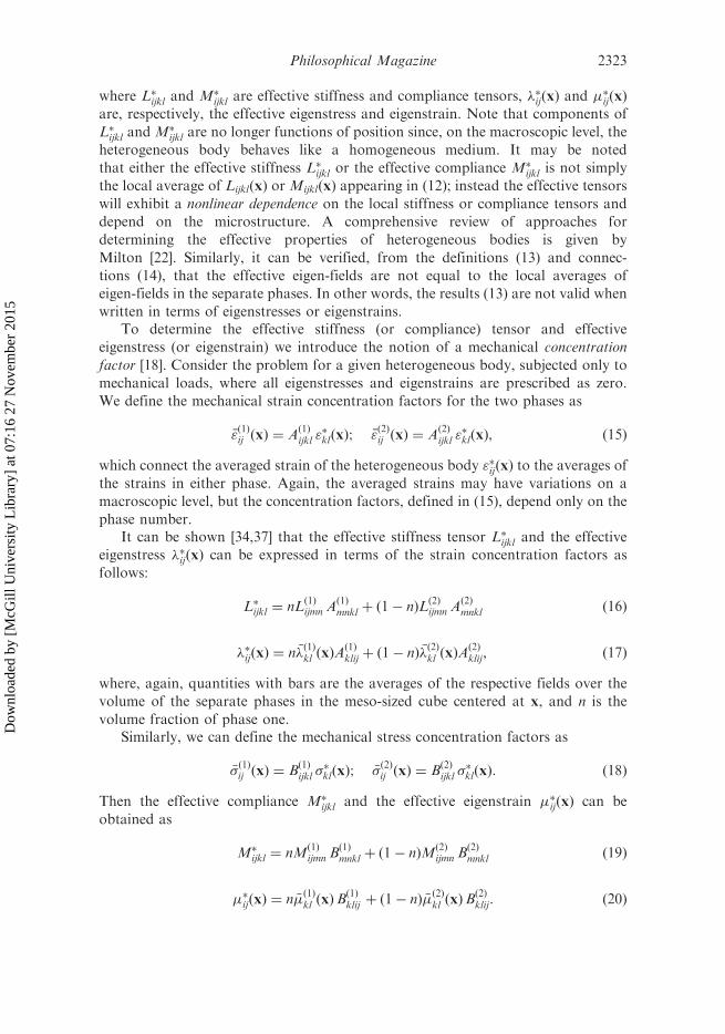
Consider an example of a geomaterial specimen of porosity n subjected to the

displacements ui ¼ "Vxi=3 on the boundary (Figure 2). Here, "V is a given constant,

equal to the prescribed volumetric strain. It can be shown that this strain is equal to

the averaged strain "V ¼ "�ii. The objective is to derive volumetric concentration

factors for the solid phase and for the pores. Assume that the deformation of the

geomaterial takes place under fully drained conditions. Also, assume that the

effective bulk modulus of the geomaterial under drained conditions is known and

equal to KD. The bulk modulus of the solid phase is denoted by Ks.From (15), the volumetric concentration factor relates the averaged volumetric

strain "V to the averages of the volumetric strains of the solid and void phases:

"Vp ¼ Ap"V; "Vs ¼ As"V, ð23Þ

where Ap, As are the (volumetric) concentration factors for the pores and the solid

phases, respectively, and "Vp, "Vs are the averages of the volumetric strains in the

pores and the solid phases, respectively (Here we often omit bars and stars for the

averaged quantities). Since the prescribed averaged strain "V is uniform, the local

averaged strain fields are also uniform, i.e. not functions of the macroscopic

coordinate x (which makes this problem convenient for obtaining the concentration

factors). From (21) the relationship between concentration factors is

nAp þ ð1� nÞAs ¼ 1: ð24Þ

Figure 2. Porous media under fully drained conditions subjected to displacements derivedfrom a uniform volumetric strain field "V.


Dow

nloa

ded

by [

McG

ill U

nive

rsity

Lib

rary

] at

07:

16 2

7 N

ovem

ber

2015

If we denote �I ¼ �kk=3 as the isotropic part of a stress tensor �ij, then, we can write

"V ¼ K�1D ��I ¼ K�1D ð�npþ ð1� nÞ�IsÞ ¼ K�1D ð1� nÞ�Is ¼ K�1D ð1� nÞKs"Vs, ð25Þ

where �Is is the average of the isotropic stress in the solid phase and p is the pressure(equal to zero under fully drained conditions). The first relationship follows from theeffective constitutive relation for an isotropic solid (14), while the second is due to thedefinition of the averaged stress ��ij in (13). In the last relationship in (25), the localconstitutive relation for the solid phase is used. Thus, from (25) and (23), one obtainsthe strain concentration factor for the solid phase:

As ¼1

1� n

KD

Ks: ð26Þ

The strain concentration factor for the pore space follows from (24):

Ap ¼1

n1�

KD

Ks

� �: ð27Þ

We can now derive the stress concentration factors: the isotropic stress concentrationfactors are defined as

�Ip ¼ Bp ��I ; �Is ¼ Bs �

�I : ð28Þ

Note that if the stress in the pores (or pore fluid pressure) is zero, then from (28) theconcentration factor for the pores Bp is also zero. Thus, from the relationship (22)

Bs ¼1

1� nð29Þ

the volumetric concentration factors derived here will be used in the subsequentsection.

4. Constitutive relationships for a partially saturated poroelastic medium

In this section, we apply the eigenstrain-stress approach for a heterogeneous mediumto re-derive the constitutive relationships (1), the void occupancy Equation (5) andthe governing equations for a partially saturated porous medium.

The saturation is defined as

s ¼Vf

Vp; s 2 ð0, 1Þ, ð30Þ

where Vf is the volume of the fluid and Vp is the pore volume.If s ¼ 1, the porous medium is fully saturated. Note that

1� s ¼Va

Vp, ð31Þ

where Va is the volume of air in the pore space.The material of the solid phase is considered to be linear elastic and compressible.

The fluid is assumed to be non-viscous and compressible. The derivation allows for


Dow

nloa

ded

by [

McG

ill U

nive

rsity

Lib

rary

] at

07:

16 2

7 N

ovem

ber

2015

thermal deformation of both the solid grains and the fluid to account for heating(cooling) of the porous medium. The derivation can be extended or modified if otherforms of eigenstresses or eigenstrains are present in the porous medium (for example,swelling, change of molecular structure of the phases, inelastic strains).

4.1. Effective stress–strain relations

As mentioned previously, the constitutive relations are expressed in terms of theelastic properties of the geomaterial under drained conditions. Thus, all eigenstressesor eigenstrains must be applied to the porous medium under drained conditions.By applying these eigen-fields, we should be able to simulate the behavior of theporous medium under general, not necessarily drained conditions (Figure 1).Following the general form of the effective stress-strain relation (14) in the presenceof eigen-fields, the total stress in the isotropic porous medium can be expressed as


3

� �"V�ij þ �T�ij þ �P�ij þ other eigenstresses, ð32Þ

where "ij are the strain components; KD, GD are the bulk and shear moduli,respectively, of the soil under drained conditions; �T is the effective eigenstress due totemperature change, and �P is the effective eigenstress due to the existence of fluidpressure. In the following, we omit all bars or superscripts-stars for both the averagedfields and the effective properties. Note that all fields in (32) are, in general, functionsof position x and time.

We now obtain �T and �P. When the temperature change T is applied to the solidphase, the thermal (volumetric) eigenstrain in the solid phase is �s ¼ 3�sT. It followsfrom the relationship between eigenstresses and eigenstrains (11) that the thermaleigenstress in the solid phase is �s ¼ �Ks3�sT, where Ks is the bulk modulus of thesolid phase (Figure 1b). To convert this local eigenstress to the effective eigenstress,applied to the drained soil, we use the result (17) [34]:

�T ¼ ð1� nÞAs�s, ð33Þ

where As is the (volumetric) strain concentration factor for the solid grains and n isthe porosity. The concentration factor As was derived in Section 3, and it is given bythe formula (26); thus, the effective eigenstress due to a temperature change in thesolid phase is

�T ¼ ð1� nÞAs½�Ks3�sT� ¼ �KD 3�sT: ð34Þ

Next, the total stress applied to the pore space is �spf � ð1� sÞ pa ¼ �sp if thepressure in the air phase pa and the surface tension at the air-fluid interface areneglected. Thus, �sp is the local eigenstress applied to the pores of the drainedmaterial (see Figure 1b for the case s ¼ 1). The capillary pressure, defined as thedifference between the pressure in the air and the fluid, is now equal to the fluidpressure multiplied by �1, i.e. pc ¼ pa � pf ¼ �p.

To convert this local eigenstress to the effective eigenstress, applied to the drainedskeleton, we make use of the result (17), which gives

�P ¼ �nAf sp, ð35Þ


Dow

nloa

ded

by [

McG

ill U

nive

rsity

Lib

rary

] at

07:

16 2

7 N

ovem

ber

2015

where Af is the (volumetric) strain concentration factor for the pore. Note that the

negative sign in (35) implies that the pressure is positive when the fluid is in

compression. From (27):

Af ¼ Ap ¼1

n1�

KD

Ks

� �

and, hence, the effective eigenstress due to the existence of pressure in the liquid is

�P ¼ � 1�KD

Ks

� �sp: ð36Þ

Substituting (34) and (36) into (32) leads to the final form of the

thermo-poroelastic constitutive relation for a partially-saturated porous medium as


3

� �"V�ij � 3KD�sT�ij � 1�

KD

Ks

� �sp: ð37Þ

Usually, if the solid phase is locally incompressible, KD � Ks and the Biot

parameter � ¼ 1� KD=Ks � 1. However, this assumption may not be valid if the

porosity n is small, even if the solid phase is incompressible; it can be shown that

n � � � 1 [38].To obtain the first governing equation, the standard equations of equilibrium and

the strain-displacement relations are used. In the absence of body forces, the

equilibrium equations are

�ij, j ¼ 0: ð38Þ

The strain components "ij are related to the displacement components ui by

"ij ¼1

2ðui,j þ uj,iÞ ð39Þ

with "V ¼ "ii ¼ ui,i. Using (37) and (39), the equilibrium Equation (38) can be

written as

KD þGD

3

� �uk,ki þ GDui,kk � KD3�sT,i � 1�

KD

Ks

� �ðspÞ,i ¼ 0: ð40Þ

The dependent variables are the displacement components ui, the pressure p and

the temperature T.

4.2. Void occupancy equation

To derive the void occupancy equation, we use the local constitutive equations (12)

for the solid phase and the liquid phase under general conditions. The notion of the

geomaterial under drained conditions is not used here. The normal isotropic stress in

the liquid phase is equal to �p and thus �p=Kf is the volumetric strain in the liquid

phase if all eigenstrains are zero. In the presence of the thermal eigenstrain and


Dow

nloa

ded

by [

McG

ill U

nive

rsity

Lib

rary

] at

07:

16 2

7 N

ovem

ber

2015

the change in the liquid mass, the volumetric strain in the fluid becomes

"Vf ¼ �p

Kfþ 3�fTþ

Dmf

mf, ð41Þ

where Dmf=mf is the eigenstrain associated with a loss or gain of liquid mass Dmf.The strain in the fluid is not the only strain in the pores. One must also take into

account the volumetric strain of air:

"Va ¼DVa

Va, ð42Þ

where Va is the initial volume of air in the pores space. Let us represent this strain in

a different form:

"Va ¼DVa

Va¼

DVa

ð1� sÞVp¼

DðVp � Vf Þ

ð1� sÞVp¼

DðVp � sVpÞ

ð1� sÞVp¼

DðVpð1� sÞÞ

ð1� sÞVp

¼DVp

Vpþ

1

1� sð�DsÞ ¼ "Vp þ

1

1� sð�DsÞ, ð43Þ

where Vp ¼ Va þ Vf is the volume of pores, "Vp is the volumetric strain of the entire

pore space, and Ds is the change in saturation.The volumetric strain in the solid phase is

"Vs ¼�IsKsþ 3�sT, ð44Þ

where �Is is the average of the isotropic stress in the solid phase, or phase number

two, i.e. �Is ¼ ð�ð2Þ11 þ �

ð2Þ22 þ �

ð2Þ33 Þ=3.

From (13), the averaged strain of the entire porous medium is equal to the sum of

averages of the strains in the fluid, air and solid phases, i.e.

"V ¼ ns"Vf þ nð1� sÞ"Va þ ð1� nÞ"Vs: ð45Þ

On the other hand, "V can be expressed in terms of the averaged strain of the entire

pore space "Vp and the averaged strain of the solid phase:

"V ¼ n"Vp þ ð1� nÞ"Vs: ð46Þ

Now, using (43) and (46), we obtain from (45) the following equation:

s"V ¼ ð1� nÞs"Vs þ ns"Vf � nDs: ð47Þ

This is the void occupancy equation, in a concise form, for the case of a partially

saturated porous medium. Using the expressions for the volumetric strain of the

solid grains (44) and the volumetric strain in the liquid (41), we can reduce (47) to the

result:

s"V ¼ ð1� nÞs�IsKsþ 3�sT

� �þ ns �

p

Kfþ 3�fTþ

Dmf

mf

� �� nDs: ð48Þ

We will attempt to eliminate the isotropic stress of the solid phase �Is from (48).

On the one hand, from (13) the total (isotropic) stress of the porous medium �I is

�I ¼ �nspþ ð1� nÞ�Is: ð49Þ


Dow

nloa

ded

by [

McG

ill U

nive

rsity

Lib

rary

] at

07:

16 2

7 N

ovem

ber

2015

This is true because the stress in the air phase is zero. On the other hand, from the

effective stress–strain relationship (37) it follows that this stress is

�I ¼ KD"V � 3KD�sT� 1�KD

Ks

� �sp: ð50Þ

By equating (49) and (50), the stress of the solid phase �Is can be found. Substitution

of this stress into (48) leads to, after simplification:

� nsDmf

mfþ 1�

KD

Ks

� �s"V þ ns

p

Kfþ 1�

KD

Ks� n

� �s2p

Ksþ nDs

¼ ns3�fTþ 1�KD

Ks� n

� �s3�sT: ð51Þ

To verify Equation (51), consider a special case of a fully saturated porous

medium with very low permeability. The pores are filled with, in general, a

compressible liquid. Under such conditions, the liquid mass remains constant and,

thus, Dmf ¼ 0. Assume that the temperature change is uniform and that the thermal

expansion coefficients of the solid phase and the liquid are equal, giving �fT ¼ �sT.Also, the external boundary of the porous body is free of any tractions or stresses.

Under these conditions, the stresses in the solid phase and the pressure p in the liquid

are zero. From Equation (51), one can then obtain ð1� KD

KsÞ"V ¼ ð1�

KD

KsÞ3�T or

"V ¼ 3�T. This means that the volumetric strain of the porous medium is equal to

the applied thermal eigenstrain, which is the expected result.It can be shown that the eigenstrain due to the change of fluid mass is

Dmf

mf¼ �

Z t

0

vl, l dt, ð52Þ

where vl,l is the divergence of the fluid velocity vector v. Note that the divergence of

the velocity in (52) cannot be obtained by taking a time derivative of the fluid strain

(41). The velocity in (52) is the velocity of the fluid entering and exiting the control

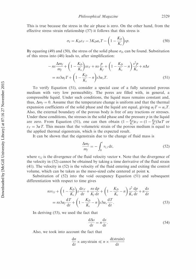
volume, which can be taken as the meso-sized cube centered at point x.Substitution of (52) into the void occupancy Equation (51) and subsequent

differentiation with respect to time gives

nsvl,l þ 1�KD

Ks

� �sd"Vdtþ

ns

Kf

dp

dtþ 1�

KD

Ks� n

� �s2

Ks

dp

dtþ n

ds

dt

¼ ns3�fdT

dtþ 1�

KD

Ks� n

� �s3�s

dT

dt: ð53Þ

In deriving (53), we used the fact that

dDsdt¼ n

ds

dt: ð54Þ

Also, we took into account the fact that

dn

dt� anystrain� n�

dðstrainÞ

dt


Dow

nloa

ded

by [

McG

ill U

nive

rsity

Lib

rary

] at

07:

16 2

7 N

ovem

ber

2015

and

ds

dt� any strain� s�

dðstrainÞ

dt;

dn

dt� Ds� n

dDsdt

;

usually, the derivative of saturation with respect to time is represented as

ds

dt¼

ds

dp

dp

dtð55Þ

and the dependence of the saturation on pressure sð pÞ for negative pressure p5 0 isgiven. Note that sð pÞ has the following properties: sð pÞ ¼ 1 for positive pressurep 0, i.e. when the porous medium is fully saturated, the pressure is non-negative.Also, ðds=dpÞ ¼ 0 if s ¼ 1 and ðds=dpÞ ¼ 0 for s! 0. The typical form of thefunction sð pÞ is shown in Figure 3.

Using (55), the void occupancy Equation (53) can be rewritten as

nsvl,l þ 1�KD

Ks

� �sd"Vdtþ

ns

Kf

dp

dtþ 1�

KD

Ks� n

� �s2

Ks

dp

dtþ n

ds

dp

dp

dt:

¼ ns3�fdT

dtþ 1�

KD

Ks� n

� �s3�s

dT

dtð56Þ

4.3. Darcy’s Law

For the case of a partially saturated medium, Darcy’s Law can be written as

nsvl ¼ �kkrelðsÞ

�p,l, ð57Þ

where krelðsÞ is the relative permeability, 0 � kre l � 1 with the property thatkrelð1Þ ¼ 1 and krelð0Þ ¼ 0. Substituting Darcy’s Law (57) into the void occupancy,Equation (56) gives the governing equation for the displacement components and thepressure:

�nskkrelðsÞ

�nsp,l

� �,l

þ�sduk,kdtþns

Kf

dp

dtþð��nÞ

s2

Ks

dp

dtþn

ds

dp

dp

dt¼ ns3�f

dT

dtþð��nÞs3�s

dT

dt,

ð58Þ

Figure 3. Dependence of saturation on fluid pressure.


Dow

nloa

ded

by [

McG

ill U

nive

rsity

Lib

rary

] at

07:

16 2

7 N

ovem

ber

2015

where the dependent variables are the displacement components ui, the pressure p

and the temperature T. Note that to solve the governing equations for the case of apartially saturated medium, it is necessary to provide dependence of saturation on

pressure sð pÞ for negative values of pressures, i.e. when 0 � s5 1.Finally, the heat conduction equation can be solved to obtain the variation of

temperature T on a macroscale:

c�p@T

@t� k�cT,kk ¼ 0, ð59Þ

where c�p is the effective specific heat of the porous medium and k�c is the effective

thermal conductivity. This equation can be derived from Fourier’s law (7) and thethermal energy balance equation. Both c�p and k�c are evaluated for a partially

saturated porous medium, i.e. c�p ¼ sncf�f þ ð1� nÞcs�s, k�c ¼ snkf þ ð1� nÞks if the

density and thermal conductivity of the air phase are neglected. Note that definition

of k�c is consistent with the fact that the temperature field is assumed equal in boththe pore space and the solid phase.

One of the advantages of using the eigenstrain-stress approach is the possibility

to compute the averaged strains and stresses in the pores (local fields) knowing theoverall strains and stresses. Consider the case of a fully saturated porous medium.Insertion of the eigenstrain

Dmf

mffound from (51) into (41) gives the averaged

volumetric strain in the pore space "Vf as

"Vf ¼�

n"V þ

�� n

n

p

Ks�� n

n3�sT: ð60Þ

Note that all quantities on the right side of this equation are the macro-scale fieldsfound by solving equations of poroelasticity.

Equation above can be generalized so that all strain components in the pore

space (phase 1) can be found in terms of the components of the overall strain,pressure and temperature fields:

"ð1Þij ¼ Að1Þijkl"kl þ ðIijkl � A

ð1ÞijklÞ�sT�kl � ðIijkl � A

ð1ÞijklÞM

ð2Þklmnp�mn, ð61Þ

where Að1Þijkl is the strain concentration factor for the pore space under drained

conditions, Mð2Þijkl is the elastic compliance matrix for the solid phase. The strain

concentration factor can be estimated by using one of the effective medium methods,such as Mori–Tanaka method.

It is important to note that the constitutive Equation (37) also can be written in

terms of the bulk and shear moduli of the undrained porous material, i.e. Ku, definedin (4), and Gu ¼ GD, respectively. Substitution of the fluid pressure from (51) into the

stress–strain Equation (37) leads to

�ij ¼ 2GD"ij þ Ku �2GD

3

� �"V�ij � ðKu �Q�nÞ3�sT�ij �Q�n 3�fTþ

Dmf

mf

� ��ij, ð62Þ

where Q ¼ 1=ð nKfþ ��n

KsÞ: Here ð3�fTþ

Dmf

mfÞ is the volumetric eigenstrain applied to the

liquid phase of the porous medium in the undrained state, and 3�sT is the volumetric

eigenstrain in the solid phase. According to the eigenstrain-stress theory,temperature-related terms in the last equation can be reduced to �3Ku�

�uT�ij,


Dow

nloa

ded

by [

McG

ill U

nive

rsity

Lib

rary

] at

07:

16 2

7 N

ovem

ber

2015

where ��u is the overall thermal expansion coefficient of a fluid-saturated porous

medium. Now we can define ��u ¼ K�1u ½ðKu �Q�nÞ�s þQ�n �f �.

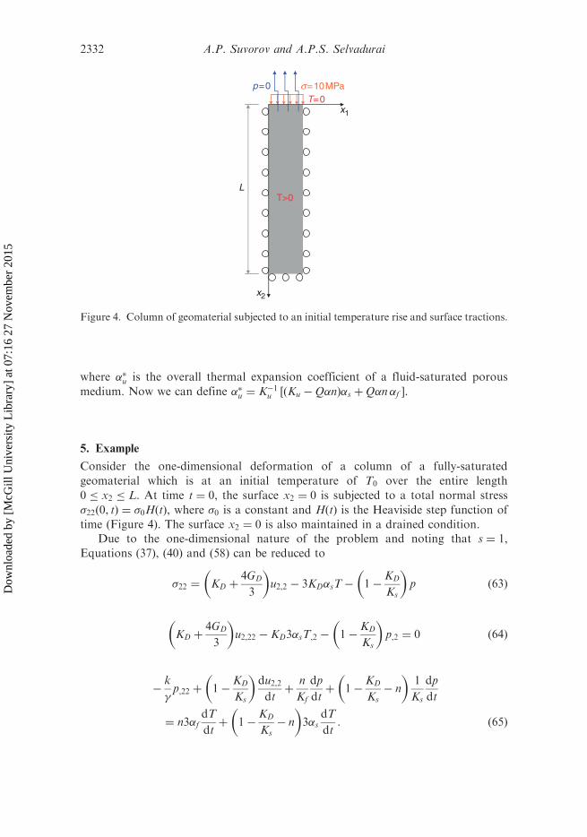
5. Example

Consider the one-dimensional deformation of a column of a fully-saturated

geomaterial which is at an initial temperature of T0 over the entire length

0 � x2 � L. At time t ¼ 0, the surface x2 ¼ 0 is subjected to a total normal stress

�22ð0, tÞ ¼ �0HðtÞ, where �0 is a constant and HðtÞ is the Heaviside step function of

time (Figure 4). The surface x2 ¼ 0 is also maintained in a drained condition.Due to the one-dimensional nature of the problem and noting that s ¼ 1,

Equations (37), (40) and (58) can be reduced to

�22 ¼ KD þ4GD

3

� �u2,2 � 3KD�sT� 1�

KD

Ks

� �p ð63Þ

KD þ4GD

3

� �u2,22 � KD3�sT,2 � 1�

KD

Ks

� �p,2 ¼ 0 ð64Þ

�k

�p,22 þ 1�

KD

Ks

� �du2,2dtþ

n

Kf

dp

dtþ 1�

KD

Ks� n

� �1

Ks

dp

dt

¼ n3�fdT

dtþ 1�

KD

Ks� n

� �3�s

dT

dt: ð65Þ

T=0s=10MPa p=0

T>0

x1

x2

L

Figure 4. Column of geomaterial subjected to an initial temperature rise and surface tractions.


Dow

nloa

ded

by [

McG

ill U

nive

rsity

Lib

rary

] at

07:

16 2

7 N

ovem

ber

2015

Suppose that the initial temperature within the column is T0, i.e.

Tðx2, t ¼ 0Þ ¼ T0: ð66Þ

The temperature of the upper surface is reduced to zero at time t ¼ 0 and the heat

flux at the base of the column x2 ¼ L is kept equal to zero, i.e.

Tðx2 ¼ 0, tÞ ¼ 0@T

@x2ðx2 ¼ L, tÞ ¼ 0: ð67Þ

The temperature field satisfying the heat conduction Equation (59), the boundary

conditions (67), and the initial condition (66) is given by [39,40]

Tðx2, tÞ ¼ T0

Xm¼1,3,5

4

msin

m

2Lx2

� �expð�2mtÞ 2m ¼

m22

4L2

k�cc�p: ð68Þ

Suppose that the tractions applied on the upper surface are equal to a

constant �0, i.e.

�22ð0, tÞ ¼ �0: ð69Þ

The equations of equilibrium (38) for this one-dimensional problem reduce to

�22,2 ¼ 0 and, hence, the total stress �22 is uniform and equal to �0 for all points

within the column.Then, from Equation (63), the strain within the column can be determined as

"22ðx2Þ ¼ u2,2 ¼1

KD þ43GD

�0 þ 1�KD

Ks

� �pþ 3KD�sT

� �: ð70Þ

Substitution of this strain into the governing Equation (65) leads to the differential

equation for the pressure:

�k

�p,22 þ

n

Kfþ ð�� nÞ

1

Ksþ

�2

KD þ43GD

" #dp

dt

¼ nð3�f ÞdT

dtþ �� n� �

KD

KD þ43GD

!ð3�sÞ

dT

dt: ð71Þ

Since the fluid can flow freely in and out through the upper surface, the pressure on

the upper surface x2 ¼ 0 is taken as equal to zero:

pðx2 ¼ 0, tÞ ¼ 0: ð72Þ

At the base x2 ¼ L, the velocity is set equal to zero:

k

�

@p

@x2ðx2 ¼ L, tÞ ¼ 0: ð73Þ

We assume that both the general solution of the homogeneous version

of (71) and a particular solution of (71) satisfy these boundary conditions.


Dow

nloa

ded

by [

McG

ill U

nive

rsity

Lib

rary

] at

07:

16 2

7 N

ovem

ber

2015

Solution of the homogeneous equation takes the form:

pHðx2, tÞ ¼X

m¼1,3,5

Cm sinm

2Lx2

� �expð�!2

mtÞ

!2m ¼

k

�

m22

4L2

KD þ43GD

ð nKfþ ð�� nÞ 1Ks

ÞðKD þ43GDÞ þ �2

,

ð74Þ

where Cm are constants to be determined.The particular solution of (71) is given as

pPðx2, tÞ ¼X

m¼1,3,5

Am4

msin

m

2Lx2

� �expð�2mtÞ

2m ¼m22

4L2

k�cc�p

,

ð75Þ

where Am are unknown constants. The solution of (71) is the sum p ¼ pH þ pP. The

constants Am can be found by substitution of pP (75) and the temperature field (68)

into the equation for the pressure (71). This gives

Am ¼ �T0

ðn3�f þ ð�� nÞ3�s ��KD

KDþ4GD=33�sÞ

k�

c�pk�c� ð nKf

þ ð�� nÞ 1Ksþ �2

KDþ4GD=3Þ: ð76Þ

Thus, it has been shown that Amð¼ AÞ is independent of m.It is now necessary to find the unknown constants Cm, which can be determined

from the initial condition on the pressure field:

pðx2, 0Þ ¼ p0, ð77Þ

where p0 is an as yet unknown initial pressure.Since

Xm¼1,3,5

4

msin

m

2Lx2

� �¼ 1 ð78Þ

and since p ¼ pH þ pP, we can establish that

p04

m¼ Cm þ Am

4

m, ð79Þ

where p0 is the initial pressure. Equation (79) allows us to find the constants Cm.Therefore, the total solution of (71) is

pðx2, tÞ ¼ p0X

m¼1,3,5,

4

msin

m

2Lx2

� �expð�!2

mtÞ �X

m¼1,3,5,

Am4

msin

m

2Lx2

� �expð�!2

mtÞ

þX

m¼1,3,5

Am4

msin

m

2Lx2

� �expð�2mtÞ: ð80Þ

To find the initial pressure p0 we use the constitutive Equation (63) and the void

occupancy Equation (51). Equating the normal stresses �22 to the applied stress �0,


Dow

nloa

ded

by [

McG

ill U

nive

rsity

Lib

rary

] at

07:

16 2

7 N

ovem

ber

2015

we obtain

KD þ4

3GD

� �"V � KD3�sT0 � �p0 ¼ �0

� nDmf

mfþ 1�

KD

Ks

� �"V þ n

p0Kfþ 1�

KD

Ks� n

� �p0Ks¼ n3�fT0 þ 1�

KD

Ks� n

� �3�sT0:

ð81Þ

By setting the initial change in the fluid mass equal to zero Dmf

� t¼0¼ 0 , we can

obtain the initial pressure from (81):

p0 ¼ ��0

�2 þ ð nKfþ ��n

KsÞðKD þ

43GDÞ

þKD þ

43GD

� ½ð�� nÞ3�sT0 þ n 3�fT0� � KD3�sT0�

�2 þ ð nKfþ ��n

KsÞðKD þ

43GDÞ

: ð82Þ

This formula is simplified if the solid phase is incompressible, i.e. Ks !1, � ¼ 1.

In this case, the initial pressure becomes

p0 ¼ ��0

1þ nKfðKD þ

43GDÞ

þðKD þ

43GDÞ½ð1� nÞ3�sT0 þ n 3�fT0� � KD3�sT0

1þ nKfðKD þ

43GDÞ

: ð83Þ

The vertical displacement can be found by integrating the normal strain (70):

u2 ¼

Z�0 þ �pþ 3KD�sT

KD þ 4GD=3dx2 þU, ð84Þ

where U is a constant of integration which can be found from the boundary

condition at the base:

u2ðL, 0Þ ¼ 0: ð85Þ

Substitution of the pressure field (80) and the temperature field (68) into

Equation (84) gives the vertical displacement:

u2 ¼1

KD þ 4GD=3�KD3�sT0

Xm¼1,3,5...

8L

m22cos

m

2Lx2

� �expð�2mtÞ

"

� �p0X

m¼1,3,5,

8L

m22cos

m

2Lx2

� �expð�!2

mtÞ

þ �X

m¼1,3,5...

Am8L

m22cos

m

2Lx2

� �expð�!2

mtÞ

� �X

m¼1,3,5...

Am8L

m22cos

m

2Lx2

� �expð�2mtÞ þ �0ðx2 � LÞ

#, ð86Þ

where the initial pressure is given by (83), the coefficient !m by (74), the coefficient mby (75), and the coefficient Am is found from (76). Note that the initial displacement


Dow

nloa

ded

by [

McG

ill U

nive

rsity

Lib

rary

] at

07:

16 2

7 N

ovem

ber

2015

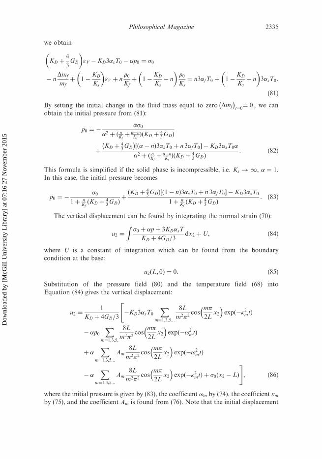
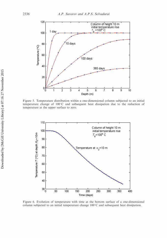
Figure 6. Evolution of temperature with time at the bottom surface of a one-dimensionalcolumn subjected to an initial temperature change 100C and subsequent heat dissipation.

Figure 5. Temperature distribution within a one-dimensional column subjected to an initialtemperature change of 100C and subsequent heat dissipation due to the reduction oftemperature at the upper surface to zero.


Dow

nloa

ded

by [

McG

ill U

nive

rsity

Lib

rary

] at

07:

16 2

7 N

ovem

ber

2015

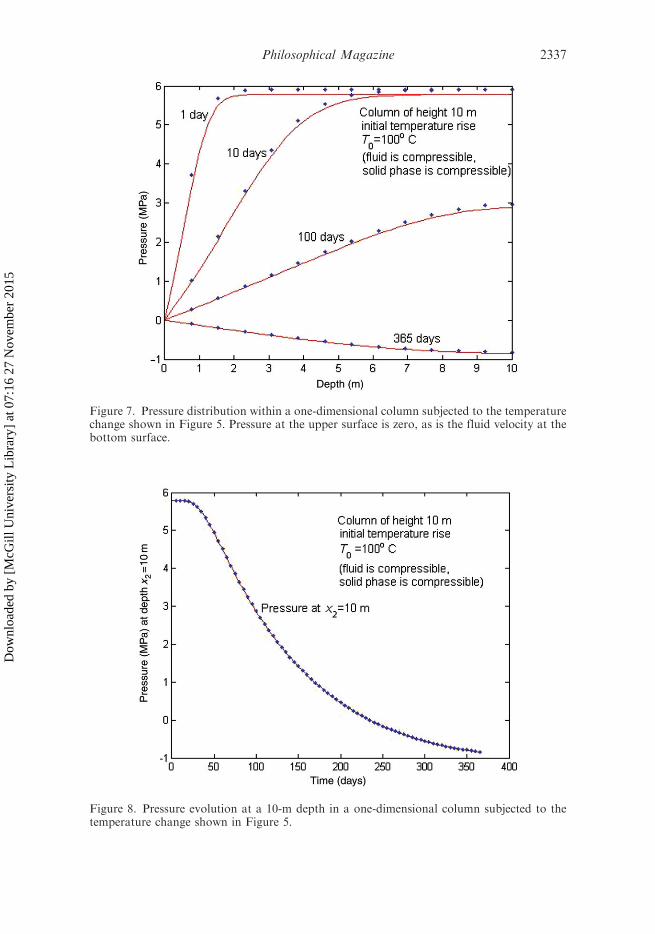
Figure 7. Pressure distribution within a one-dimensional column subjected to the temperaturechange shown in Figure 5. Pressure at the upper surface is zero, as is the fluid velocity at thebottom surface.

Figure 8. Pressure evolution at a 10-m depth in a one-dimensional column subjected to thetemperature change shown in Figure 5.


Dow

nloa

ded

by [

McG

ill U

nive

rsity

Lib

rary

] at

07:

16 2

7 N

ovem

ber

2015

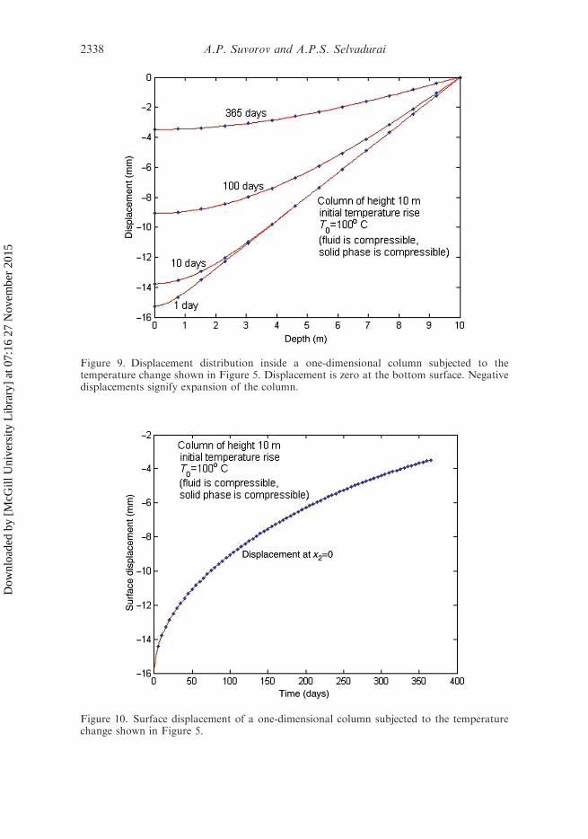
Figure 9. Displacement distribution inside a one-dimensional column subjected to thetemperature change shown in Figure 5. Displacement is zero at the bottom surface. Negativedisplacements signify expansion of the column.

Figure 10. Surface displacement of a one-dimensional column subjected to the temperaturechange shown in Figure 5.


Dow

nloa

ded

by [

McG

ill U

nive

rsity

Lib

rary

] at

07:

16 2

7 N

ovem

ber

2015

Figure 12. Surface displacement of a one-dimensional column subjected to a compressive loadof 10MPa at the upper surface. Positive displacements signify contraction of the column.

Figure 11. Pressure distribution at a 10-m depth in a one-dimensional column subjected to acompressive load of 10MPa at the upper surface.


Dow

nloa

ded

by [

McG

ill U

nive

rsity

Lib

rary

] at

07:

16 2

7 N

ovem

ber

2015

is given by

u2ðx2, t ¼ 0Þ ¼L

KD þ 4GD=31�

x2L

� �½�KD3�sT0 � �p0 � �0� ð87Þ

since Xm¼1,3,5,

8L

m22¼ L:

The time-dependent or transient response of a poroelastic column of height Lsubjected to the initial temperature change T0 and constant surface tractions �0(Figure 4) is illustrated in Figures 5–12. The specific values of the height, bulkmodulus under drained conditions, the applied traction and temperature changeappear in Table 1; the relationship between the properties of the poroelastic columnis also shown in Table 1.

In Figures 5–12, the analytical solution is shown with a solid line, and thesolution obtained by using the finite element program COMSOL is shown as adotted line (the same results can be obtained by using the finite element programABAQUS). When using either ABAQUS or COMSOL, it is not necessary to specifythe initial pressure as it can be set equal to zero.

6. Conclusions

An alternative derivation of the constitutive equations for a porous thermoelasticmedium is presented. The derivation is based on the eigenstrain-stress approach andbasic principles of micromechanics of a heterogeneous material conventionallyidentified with composite materials. The constitutive equations can be extended toinclude other forms of eigenstresses or eigenstrains, besides the thermal eigenstrain,existing in the porous medium (for example, swelling, eigenstrains associated withthe change of molecular structure of the phases, inelastic deformation).

Acknowledgements

The work described in the paper was supported in part by an NSERC Discovery Grantawarded to A.P.S. Selvadurai. The authors are grateful to a reviewer for constructivecomments.

Table 1. Specific values of the geometric and physical parameters of ageomaterial whose transient response is shown in Figures 5–12.

Name of variableor parameter Value

Name of variableor parameter Value

L 10m KD þ43GD

� =Kf 36.7133

KD 50GPa Biot parameter � 0.75�s ¼ �f 8.3E-6 1/C Porosity n 0.25�0 �10MPa

k�cc�p

1L2 1.6227E-8 [1/sec]

T0 100C k�ðKDþ4GD=3Þ

L2 2.4231E-7 [1/sec]KD þ

43GD

� =KD 1.6154


Dow

nloa

ded

by [

McG

ill U

nive

rsity

Lib

rary

] at

07:

16 2

7 N

ovem

ber

2015

Key symbols

n porosity, ratio of volume of pores to the total volume of soil Vp=VKD bulk modulus of drained soilGD shear modulus of drained soilKs bulk modulus of solid grainsKf bulk modulus of fluid�s linear thermal expansion coefficient of solid grains�f linear thermal expansion coefficient of liquid"V volumetric strain of soil"ij strain components�ij stress componentsp pressurek hydraulic conductivity� unit weight of liquidv fluid velocityT temperature change

References

[1] M.A. Biot, J. Appl. Phys. 12 (1941) p.155.[2] A.E. Scheidegger, Appl. Mech. Rev. 13 (1960) p.313.

[3] G. Paria, Appl. Mech. Rev. 16 (1963) p.901.[4] J.R. Rice and M.P. Cleary, Rev. Geophys. Space Phys. 14 (1976) p.227.[5] A.P.S. Selvadurai (ed.), Mechanics of Poroelastic Media, Kluwer Academic,

The Netherlands, 1996.

[6] A.P.S. Selvadurai, Appl. Mech. Rev. 60 (2007) p.87.[7] O. Coussy, J. Mech. Phys. Solids 53 (2005) p.1689.[8] A. Verruijt Consolidation of soils, in Encyclopedia of Hydrological Sciences,

M.G. Anderson, ed., Wiley, Chichester, UK, 2005, p.1.[9] L. Dormieux, D. Kondo and F.J. Ulm, Microporomechanics, Wiley, Chichester, UK,

2006.

[10] S.C. Cowin (ed.), Bone Mechanics Handbook, CRC Press, Boca Raton, FL, 2001.[11] M.L. Oyen, J. Mater. Res. 23 (2008) p.1307.[12] L.A. Taber, Z. Jinmei and R. Perucchio, Trans. ASME J. Biomech. Eng. 129 (2007)

p.441.

[13] M. Galli and M.L. Oyen, Comput. Model. Eng. Sci. 48 (2009) p.241.[14] Y. Abousleiman and S. Ekbote, Trans. ASME J. Appl.Mech. 72 (2005) p.102.[15] B. Berkowitz, J. Bear and C. Braester, Water Resourc. Res. 24 (1988) p.1225.

[16] A.P.S. Selvadurai and T.S. Nguyen, Comput. Geotech. 17 (1995) p.39.[17] A.P.S. Selvadurai and T.S. Nguyen, Eng. Geol. 47 (1996) p.379.[18] R. Hill, J. Mech. Phys. Solids 11 (1963) p.357.

[19] R. Hill, J. Mech. Phys. Solids 13 (1965) p.213.[20] Z. Hashin, J. Appl. Mech. 50 (1983) p.481.[21] R.M. Christensen, Mechanics of Composite Materials, Wiley, Chichester, UK, 1979.[22] G.W. Milton, The Theory of Composites, Cambridge University Press, 2002.

[23] S. Torquato, Random Heterogeneous Materials: Microstructure and Macroscopic

Properties, Springer, New York, 2002.[24] A.P.S. Selvadurai and P.A. Selvadurai, Proc. R. Soc. A 466 (2010) p.2819.[25] D.F. McTigue, J. Geophys. Res. B 91 (1986) p.9533.

[26] C. Savvidou and J.R. Booker, Int. J. Num. Anal. Methods Geomech. 13 (1989) p.75.


Dow

nloa

ded

by [

McG

ill U

nive

rsity

Lib

rary

] at

07:

16 2

7 N

ovem

ber

2015

[27] N. Khalili and A.P.S. Selvadurai, Geophys. Res. Lett. 30 (2003) p.2268; DOI:10.1029/2003GL018838.

[28] J. Rutqvist, L. Borgesson, M. Chijimatsu, A. Kobayashi, L. Jing, T.S. Nguyen,J. Noorishad and C.F. Tsang, Int. J. Rock Mech. Min. Sci. 38 (2001) p.105.

[29] R. Burridge and J.B. Keller, J. Acous. Soc. Am. 70 (1081) p.1140.[30] A. Norris, J. Appl. Phys. 71 (1992) p.1138.[31] T. Mura, Micromechanics of defects in solids, in Mechanics of Elastic and Inelastic Solids,

2nd ed., Springer, New York, 1987.[32] G.J. Dvorak, Y.A. Bahei-El-Din and A.M. Wafa, Model. Simul. Mater. Scie. Eng. A

2 (1994) p.571.

[33] X. Chateau and L. Dormieux, Int. J. Num. Anal. Methods Geomech. 26 (2002)p.831.

[34] V.M. Levin, Mech. Solids 1 (1967) p.88.

[35] A.P.S. Selvadurai, Partial Differential Equations in Mechanics, Vol. 2, The BiharmonicEquation, Poisson’s Equation, Springer, Berlin, 2000.

[36] A.J.M. Spencer, Continuum Mechanics, Dover Publications, New York, 2004.[37] V.M. Levin, Alvarez-Tostado, Arch. Appl. Mech. 76 (2006) p.199.

[38] D. Lydzba and J.F. Shao, Mech. Cohes.-Frict. Mater. 5 (2000) p.149.[39] H.S. Carslaw and J.C. Jaeger, Heat Conduction in Solids, Clarendon Press, Oxford, 1959.[40] A.P.S. Selvadurai, Partial Differential Equations in Mechanics, Vol. 1, Fundamentals,

Laplace’s Equation, Diffusion Equation, Wave Equation, Springer, Berlin, 2000.


Dow

nloa

ded

by [

McG

ill U

nive

rsity

Lib

rary

] at

07:

16 2

7 N

ovem

ber

2015

Date post:	04-Jan-2022
Category:	Documents
Upload:	others
View:	2 times
Download:	0 times

Macroscopic constitutive equations of thermo ...

Documents