MAE4700/5700 Finite Element Analysis for Mechanical...

CCOORRNNEELLLL U N I V E R S I T Y 1

MAE 4700 – FE Analysis for Mechanical & Aerospace DesignN. Zabaras (9/23/2009)

MAE4700/5700Finite Element Analysis for

Mechanical and Aerospace Design

Cornell University, Fall 2009

Nicholas ZabarasMaterials Process Design and Control Laboratory

Sibley School of Mechanical and Aerospace Engineering101 Rhodes Hall

Cornell UniversityIthaca, NY 14853-3801

http://mpdc.mae.cornell.edu/Courses/MAE4700/MAE4700.html



Finite element basis functions in 1D• The domain is divided into finite elements and the

weight functions and trial solutions are constructed within each element.

• These functions have to be chosen so that the FEM converges, i.e. as element size, denoted by h, decreases, the solution tends to the correct solution (mesh refinement).

• Convergence of the FEM requires basis functions that satisfy continuity and completeness.



Continuity and completeness• Continuity: the trial solutions and weight functions need to

be sufficiently smooth. The degree of smoothness required depends on the order of the derivatives that appear in the weak form. For the 2nd order ODEs considered, the derivatives in the weak form are 1st order, thus the weight functions and trial solutions must be H1 (C0 piecewise polynomials).

• Completeness: the basis functions need to be able toapproximate a given smooth function with arbitrary accuracy. As the element size h approaches zero, the trial solutions and weight functions and their derivatives up to, and including the highest-order derivative appearing in the weak form, must be capable of assuming constant values

finite elements can represent rigid body motion and constant strain states exactly



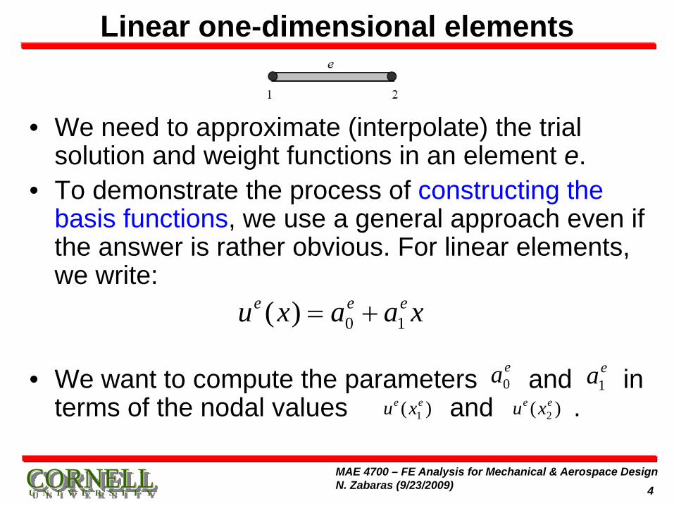
Linear one-dimensional elements

• We need to approximate (interpolate) the trial solution and weight functions in an element e.

• To demonstrate the process of constructing the basis functions, we use a general approach even if the answer is rather obvious. For linear elements, we write:

• We want to compute the parameters and in terms of the nodal values and .

0 1( )e e eu x a a x= +

0ea 1

ea1( )e eu x 2( )e eu x



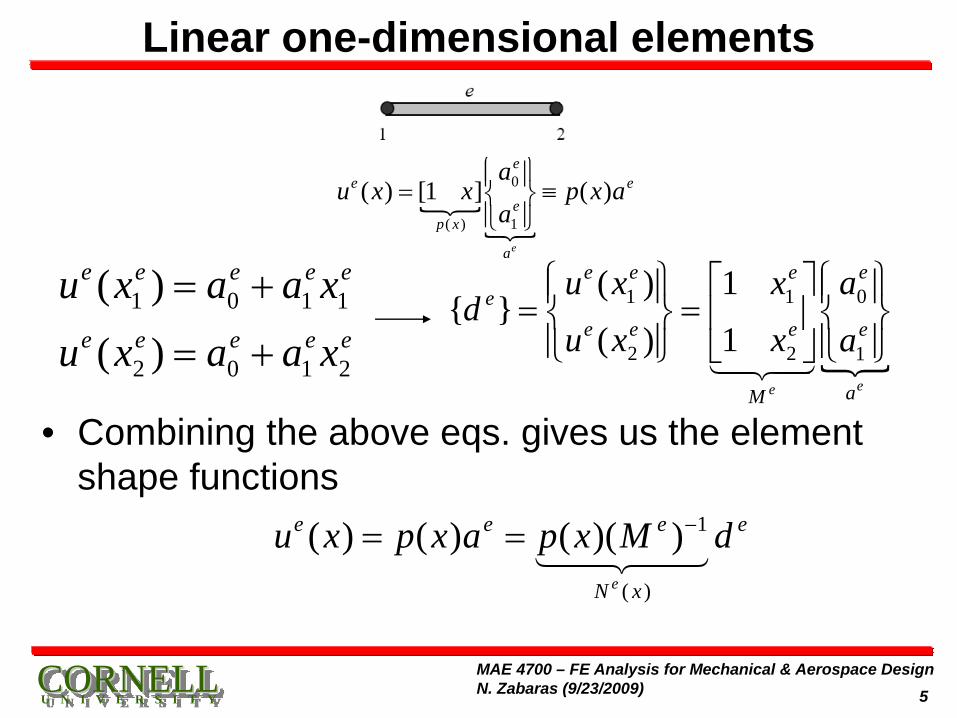
Linear one-dimensional elements

• Combining the above eqs. gives us the element shape functions

0

( ) 1

( ) [1 ] ( )

e

ee e

ep x

a

au x x p x a

a

⎧ ⎫⎪ ⎪= ≡⎨ ⎬⎪ ⎪⎩ ⎭

1 0 1 1

2 0 1 2

( )

( )

e e e e e

e e e e e

u x a a x

u x a a x

= +

= +

01 1

2 2 1

( ) 1{ }

( ) 1ee

ee e ee

e e e e

aM

au x xd

u x x a

⎧ ⎫⎧ ⎫ ⎡ ⎤⎪ ⎪ ⎪ ⎪= =⎨ ⎬ ⎨ ⎬⎢ ⎥⎪ ⎪ ⎪ ⎪⎩ ⎭ ⎩ ⎭⎣ ⎦

1

( )

( ) ( ) ( )( )e

e e e e

N x

u x p x a p x M d−= =



Element shape functions

• The element shape function matrix can now be computed as:

1 2 11 2

1[ ] ( )( ) [1 ]1 1

e ee e e e

e

x xN N N p x M x

L− ⎡ ⎤−

= = = ⇒⎢ ⎥−⎣ ⎦

1

11 2 1

2

1 1( )1 11

e

e e ee

ee

M

x x xM

Lx

−

− ⎡ ⎤ ⎡ ⎤−= =⎢ ⎥ ⎢ ⎥−⎣ ⎦⎣ ⎦

11 2 2 1

1[ ] ( )( )e e e e e eeN N N p x M x x x x

L− ⎡ ⎤= = = − − ⇒⎣ ⎦

1 2

2 1

1 ( )

1 ( )

e ee

e ee

N x xL

N x xL

= −

= −



Two-node linear element: Shape functions

• Verify that (as desired) the following holds:

• The interpolation property is now summarized as:

1 2

2 1

1 ( )

1 ( )

e ee

e ee

N x xL

N x xL

= −

= −

( )e ei j ijN x δ=

11 2 1 1 2 2

2

( ) ( ) [ ]e

e e e e e e e e ee

du x N x d N N N d N d

d

⎧ ⎫⎪ ⎪= = = + ⇒⎨ ⎬⎪ ⎪⎩ ⎭

1 1 2 22

1

( )e e e e e

e ei i

i

u x N d N d

N d=

= +

= ∑

Note:1 1 1 1 2 1 2 1 2 1

2 1 2 1 2 2 2 1 2 2

( ) ( ) ( ) 1 0

( ) ( ) ( ) 0 1

e e e e e e e e e e e

e e e e e e e e e e e

u x N x d N x d d d d

u x N x d N x d d d d

= + = + =

= + = + =



Two-node linear element: Shape functions

• The derivative of can now be approximated as:

1 21 2

( ) ( ) e ee ee e edN dNdu x dN x d d d

dx dx dx dx= = +

1 2

2 1

1 ( )

1 ( )

e ee

e ee

N x xL

N x xL

= −

= −

From which we can write:

( )eu x

{ }1

2

( ) 1 1[ ]

e

eee e

e e e

B

ddu x B ddx L L d

⎧ ⎫⎪ ⎪= − =⎨ ⎬⎪ ⎪⎩ ⎭



Three node element: quadratic interpolation

• We can repeat the same process as for the 2-node element to derive the shape functions for the 3-node element.

• However, we can use Lagrange interpolants to find out directly the shape functions using simple arguments.

• Lets derive . It’s a quadratic function, and it needs to be zero at nodes and . So it needs to be of the form: . It also needs to take a value of 1 at node . We finally arrive at:

1eN

2ex 3

ex 2 3( )( )e ex x x x− −∼1ex

2 31

1 2 1 3

( )( )( )( )

e ee

e e e e

x x x xNx x x x− −

=− −



3-node (quadratic) and 4-node (cubic) elements

• We can generalize this process to higher order interpolation. For cubic interpolation, we need 4 nodes.

2 31

1 2 1 3

1 32

2 1 2 3

1 23

3 1 3 2

( )( )( )( )

( )( )( )( )

( )( )( )( )

e ee

e e e e

e ee

e e e e

e ee

e e e e

x x x xNx x x x

x x x xNx x x x

x x x xNx x x x

− −=

− −

− −=

− −

− −=

− −

2 3 41

1 2 1 3 1 4

1 3 42

2 1 2 3 2 4

1 2 43

3 1 3 2 3 4

1 2 34

4 1 4 2

( )( )( )( )( )( )

( )( )( )( )( )( )

( )( )( )( )( )( )

( )( )( )( )( )(

e e ee

e e e e e e

e e ee

e e e e e e

e e ee

e e e e e e

e e ee

e e e e

x x x x x xNx x x x x x



x x x x x xNx x x x

− − −=

− − −

− − −=

− − −

− − −=

− − −

− − −=

− − 4 3 )e ex x−



Master elements in natural coordinate• It is more common to define the shape functions on a

master element in coordinate with .• For linear elements, we can then easily map to real

coordinate x for each element e with the isoparametric transformation (the same interpolation we used for u(x)):

ξ

1 1ξ− ≤ ≤

{ }1 2

11 2 1 1 2 1 2

2

1 1 1( )(1 )2 2 2

e e

ee e e e e e e e e

e

N N

xx x x x x x N N N x

xξ ξξ

⎧ ⎫− + ⎡ ⎤ ⎡ ⎤= + − + = + = =⎨ ⎬⎣ ⎦ ⎣ ⎦⎩ ⎭

1

2

1 (1 )21 (1 )2

e

e

N

N

ξ

ξ

= −

= +

ξ



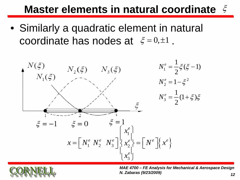
Master elements in natural coordinate

• Similarly a quadratic element in natural coordinate has nodes at .

ξ

0, 1ξ = ±

1

22

3

1 ( 1)211 (1 )2

e

e

e

N

N

N

ξ ξ

ξ

ξ ξ

= −

= −

= +

{ }1

1 2 3 2

3

e

e e e e ee

e

xx N N N N xx

x

⎧ ⎫⎪ ⎪⎡ ⎤ ⎡ ⎤= =⎨ ⎬⎣ ⎦ ⎣ ⎦⎪ ⎪⎩ ⎭



Global and element shape functions• In an earlier lecture, we introduced the transformation

from elemental to global degrees of freedom:

• By assembling the local element approximations, we can compute our global finite element approximation:

• N are our global shape functions. We can rewrite the global approximation as:

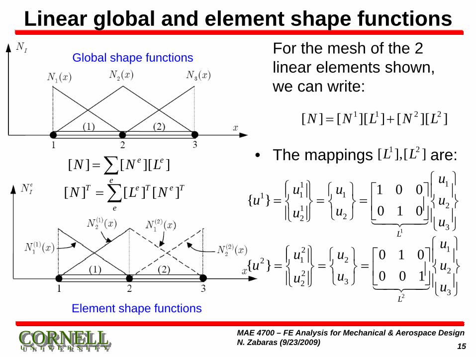
{ } [ ]{ }e ed L d=

( ) [ ]{ } [ ][ ]{ }h e e e e

e e

N

u x N d N L d= =∑ ∑

1

( ) [ ]{ }nodesN

hi i

i

u x N d N d=

= = ∑Number of nodes

in the mesh

Global shapefunctions (row matrix)



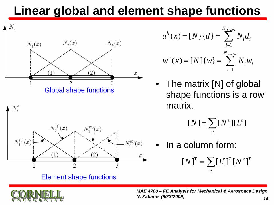
Linear global and element shape functions

• The matrix [N] of global shape functions is a row matrix.

• In a column form:

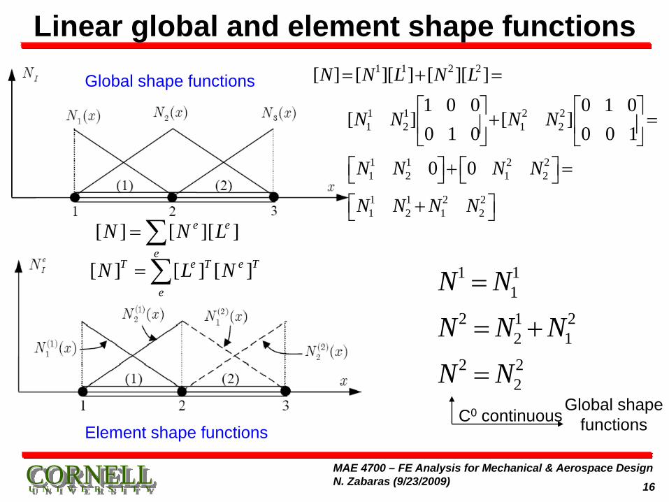
[ ] [ ][ ]e e

e

N N L=∑

1

1

( ) [ }{ }

( ) [ ]{ }

nodes

nodes

Nh

i ii

Nh

i ii

u x N d N d

w x N w N w

=

=

= =

= =

∑

∑

[ ] [ ] [ ]T e T e T

e

N L N=∑

Global shape functions




Linear global and element shape functions• For the mesh of the 2

linear elements shown, we can write:

• The mappings are:

1 1 2 2[ ] [ ][ ] [ ][ ]N N L N L= +

[ ] [ ] [ ]T e T e T

e

N L N=∑[ ] [ ][ ]e e

e

N N L=∑1 2[ ],[ ]L L

1

111 11

2122

3

1 0 0{ }

0 1 0L

uu u

u uuu u

⎧ ⎫⎧ ⎫ ⎧ ⎫ ⎡ ⎤⎪ ⎪ ⎪ ⎪= = =⎨ ⎬ ⎨ ⎬ ⎨ ⎬⎢ ⎥⎪ ⎪ ⎣ ⎦⎩ ⎭⎩ ⎭ ⎪ ⎪⎩ ⎭

2

12212

2232

3

0 1 0{ }

0 0 1L

uuu

u uuu u

⎧ ⎫⎧ ⎫ ⎧ ⎫ ⎡ ⎤⎪ ⎪ ⎪ ⎪= = =⎨ ⎬ ⎨ ⎬ ⎨ ⎬⎢ ⎥⎪ ⎪ ⎣ ⎦⎩ ⎭⎩ ⎭ ⎪ ⎪⎩ ⎭





Linear global and element shape functions1 1 2 2

1 1 2 21 2 1 2

1 1 2 21 2 1 2

1 1 2 21 2 1 2

[ ] [ ][ ] [ ][ ]1 0 0 0 1 0

[ ] [ ]0 1 0 0 0 1

0 0

N N L N L

N N N N

N N N N

N N N N

= + =

⎡ ⎤ ⎡ ⎤+ =⎢ ⎥ ⎢ ⎥

⎣ ⎦ ⎣ ⎦⎡ ⎤ ⎡ ⎤+ =⎣ ⎦ ⎣ ⎦⎡ ⎤+⎣ ⎦

[ ] [ ] [ ]T e T e T

e

N L N=∑[ ] [ ][ ]e e

e

N N L=∑1 1

12 1 2

2 12 2

2

N N

N N N

N N

=

= +

=Global shape

functionsC0 continuous





Linear global and element shape functions

Piecewise-linear basis functions for a 4-element

mesh generated by linear shape functions, defined

over each element.

eiN

iN



Quadratic global and element shape functions

A mesh consisting of three quadratic elements and the

global basis functionsgenerated by these elements.

iN



Gauss quadrature: Numerical integration• In FEM, we need to compute element stiffness and load

contributions. These are integrals that generally cannot be computed analytically.

• We need a numerical approach to computing integrals over elements in the form:

• Let us assume a linear element from to . With the transformation , we can map the integral I to natural coordinates as:

• We need a numerical approximation to integrate in .

( )e

I f x dxΩ

= ∫

1ex 2

ex1

2 21 2 1 1( )(1 ) (1 )ee e e e Lx x x x xξ ξ= + − + = + +

11

211

( ( )) ( ) , edx LdI f x Jd J f d J ξξ ξ ξ ξ

−−

= = = =∫ ∫ξ



Jacobian of the transformation from x to ξ• We just showed that for a linear element the Jacobian of

the transformation is derived as:

• Similarly for higher-order elements (n=3,4,..) using the isoparametric transformation, we derive that:

• Please note that for higher-order elements, the Jacobianof the transformation generally changes from Gauss point to Gauss point.

{ }1 2

1 1 11 2 2 11 2 1 2

2 2 2

1 1 1 12 2 2 2 2 2

e e

e e ee e e e ee e e e e e

e e e

N N

x x xdN dN x xdx Lx x x N N N x Jd d dx x x

ξ ξξ ξ ξ

⎧ ⎫ ⎧ ⎫ ⎧ ⎫⎡ ⎤ −− + ⎡ ⎤⎡ ⎤ ⎡ ⎤= + = = ⇒ ≡ = = − = =⎨ ⎬ ⎨ ⎬ ⎨ ⎬⎢ ⎥⎣ ⎦ ⎣ ⎦ ⎢ ⎥⎣ ⎦⎣ ⎦⎩ ⎭ ⎩ ⎭ ⎩ ⎭

1 1 1

2 2 21 21 2 .... ....

... ... ...

e e e

e e eee e ee e e n

n

e e en n n

x x xx x xdNdN dN dNdxx N N N J

d d d d d

x x x

ξ ξ ξ ξ ξ

⎧ ⎫ ⎧ ⎫ ⎧ ⎫⎪ ⎪ ⎪ ⎪ ⎪ ⎪

⎡ ⎤ ⎡ ⎤⎪ ⎪ ⎪ ⎪ ⎪ ⎪⎡ ⎤= ⇒ ≡ = =⎨ ⎬ ⎨ ⎬ ⎨ ⎬⎢ ⎥ ⎢ ⎥⎣ ⎦⎣ ⎦⎣ ⎦⎪ ⎪ ⎪ ⎪ ⎪ ⎪

⎪ ⎪ ⎪ ⎪ ⎪ ⎪⎩ ⎭ ⎩ ⎭ ⎩ ⎭



Gauss quadrature: Numerical integration

• are appropriate weights and are appropriate evaluation points. The selection of these is optimal in the sense that the highest possible polynomial can be integrated exactly.

• An Gauss integration formula can integrate exactly a polynomial of order

• So if you have to integrate a polynomial of order p, you need to use

int

int int

1

1 111

( ) ( ) ( ) ... ( )Gauss Po s

Gauss Po s Gauss Po s

N

i i N Ni

I f d W f W f W fξ ξ ξ ξ ξ=−

= = = + +∑∫iW iξ

intGauss Po sN

int2 1.Gauss Po sN −

int

12Gauss Po s

pN

+≥

For p=2, you need a minimum of 2 Gauss pointsFor p=3, you need a minimum of 2 Gauss points



Gauss quadrature

1 0.0 2.02 1.0

3 ±0.77459666920

0.55555555560.8888888889

4 ±0.8611363116±0.3399810436

0.34785484510.6521451549

5 ±0.9061798459±0.5384693101

0.0

0.23692688510.47862867050.5688888889

intGauss Po sN ξ iW

13

±



An example of Gauss quadrature

• Let us compute the integral:

• We need:

• Using Gauss quadrature:

1 4 2

1

2 4 26( 2 ) ( 1.73333)5 3 15

I dξ ξ ξ−

= + = + = =∫

int int

1 4 12.5 3.2 2Gauss Po s Gauss Po s

pN N

+ +≥ = = ⇒ =

1 1 2 2 3 3

1 2 3 2 1 3

1 2 3

( ) ( ) ( ),0.7745966692, 0, 0.7745966692 ( ) 0, ( ) ( ) 1.560.5555555556, 0.8888888889, 0.5555555556

I W f W f W ff f f

W W W

= + +

= = = − ⇒ = = =

= = =

ξ ξ ξξ ξ ξ ξ ξ ξ

10.5555555556 1.56 0.8888888889 0 0.5555555556 1.56 1.73333!I I= × + × + × ⇒ =

Date post:	23-May-2018
Category:	Documents
Upload:	lamphuc
View:	221 times
Download:	1 times

MAE4700/5700 Finite Element Analysis for Mechanical...

Documents