29
Magnet Issues Steve Kahn OleMiss Workshop Mar 11, 2004
| Date post: | 01-Jan-2016 |
| Category: |
Documents |
| Upload: | steel-stokes |
| View: | 35 times |
| Download: | 0 times |

Magnet Issues
Steve KahnOleMiss Workshop
Mar 11, 2004
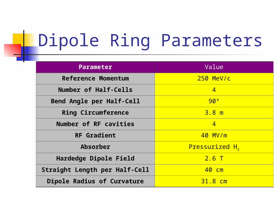
Parameter Value
Reference Momentum 250 MeV/c
Number of Half-Cells 4
Bend Angle per Half-Cell 90°
Ring Circumference 3.8 m
Number of RF cavities 4
RF Gradient 40 MV/m
Absorber Pressurized H2
Hardedge Dipole Field 2.6 T
Straight Length per Half-Cell 40 cm
Dipole Radius of Curvature 31.8 cm
Dipole Ring Parameters
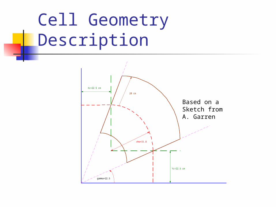
Cell Geometry Description
rho=31.8
gamma=22.5
Xc=22.5 cm
Yc=22.5 cm
20 cm
Based on a Sketch from A. Garren
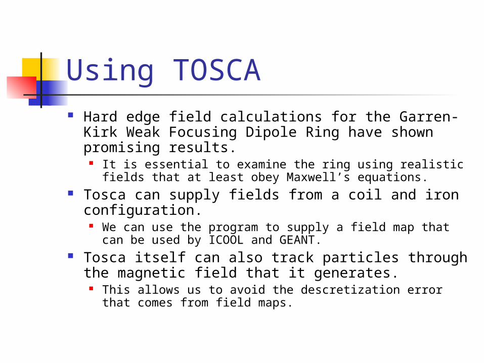
Using TOSCA Hard edge field calculations for the Garren-Kirk
Weak Focusing Dipole Ring have shown promising results. It is essential to examine the ring using realistic fields
that at least obey Maxwell’s equations. Tosca can supply fields from a coil and iron
configuration. We can use the program to supply a field map that can
be used by ICOOL and GEANT. Tosca itself can also track particles through the
magnetic field that it generates. This allows us to avoid the descretization error that
comes from field maps.
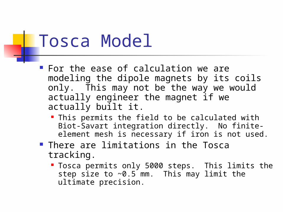
Tosca Model For the ease of calculation we are modeling
the dipole magnets by its coils only. This may not be the way we would actually engineer the magnet if we actually built it. This permits the field to be calculated with Biot-
Savart integration directly. No finite-element mesh is necessary if iron is not used.
There are limitations in the Tosca tracking. Tosca permits only 5000 steps. This limits the
step size to ~0.5 mm. This may limit the ultimate precision.
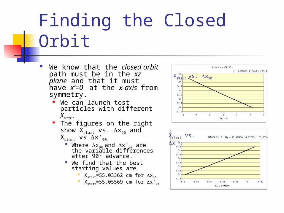
Finding the Closed Orbit We know that the closed orbit
path must be in the xz plane and that it must have x’=0 at the x-axis from symmetry. We can launch test particles
with different Xstart. The figures on the right show
Xstart vs. x90 and Xstart vs x'90. Where x90 and x'90 are the
variable differences after 90° advance.
We find that the best starting values are
Xstart=55.03362 cm for x90 Xstart=55.05569 cm for x'90
Xstart vs X90-X0
y = 0.00955x2 - 0.76870x + 55.03362
51.5
52
52.5
53
53.5
54
54.5
55
55.5
56
-1 0 1 2 3 4 5
dx, cm
Xstart, cm
Xstart vs. X' 90 y = 25.45703x 2 + 34.62725x + 55.05569
51.5
52
52.5
53
53.5
54
54.5
55
55.5
56
-0.1 -0.08 -0.06 -0.04 -0.02 0 0.02
dX', radians
Xstart, cm
Xstart vs. x90
Xstart vs. x'90
Closed Orbit
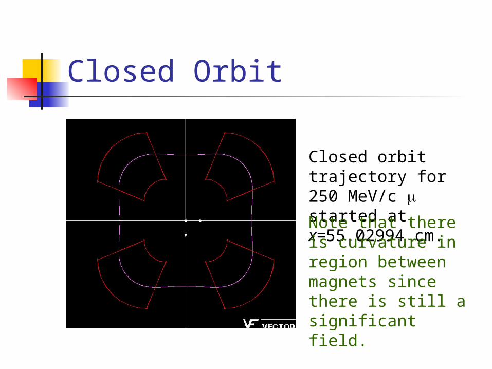
Closed orbit trajectory for 250 MeV/c started at x=55.02994 cm.
Note that there is curvature in region between magnets since there is still a significant field.
Field Along the Reference Path
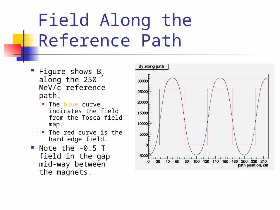
Figure shows By along the 250 MeV/c reference path. The blue curve
indicates the field from the Tosca field map.
The red curve is the hard edge field.
Note the –0.5 T field in the gap mid-way between the magnets.
Calculating Transfer Matrices By launching particles on trajectories at
small variations from the closed orbit in each of the transverse directions and observing the phase variables after a period we can obtain the associated transfer matrix. Particles were launched with
x = ± 1 mm x' = ± 10 mr y = ± 1 mm y' = ± 10 mr
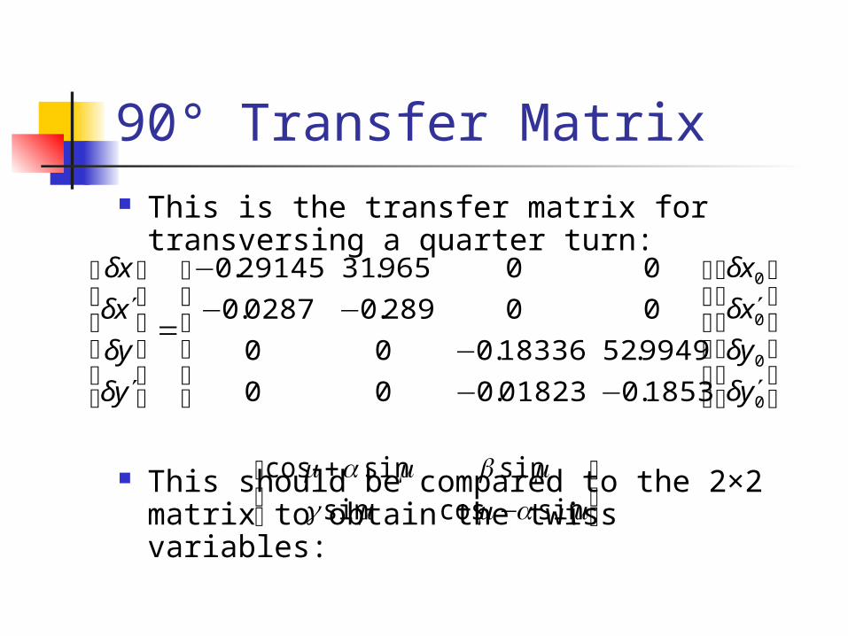
90° Transfer Matrix This is the transfer matrix for
transversing a quarter turn:
This should be compared to the 2×2 matrix to obtain the twiss variables:
⎥⎥⎥⎥
⎦
⎤
⎢⎢⎢⎢
⎣
⎡
′
′
⎥⎥⎥⎥
⎦
⎤
⎢⎢⎢⎢
⎣
⎡
−−−
−−−
=
⎥⎥⎥⎥
⎦
⎤
⎢⎢⎢⎢
⎣
⎡
′
′
0
0
0
0
1853.001823.000
9949.5218336.000
00289.00287.0
00965.3129145.0
y
y
x
x
y
y
x
x
δ
δ
δ
δ
δ
δ
δ
δ
⎥⎦
⎤⎢⎣
⎡−
+αγ
βαsincossin
sinsincos
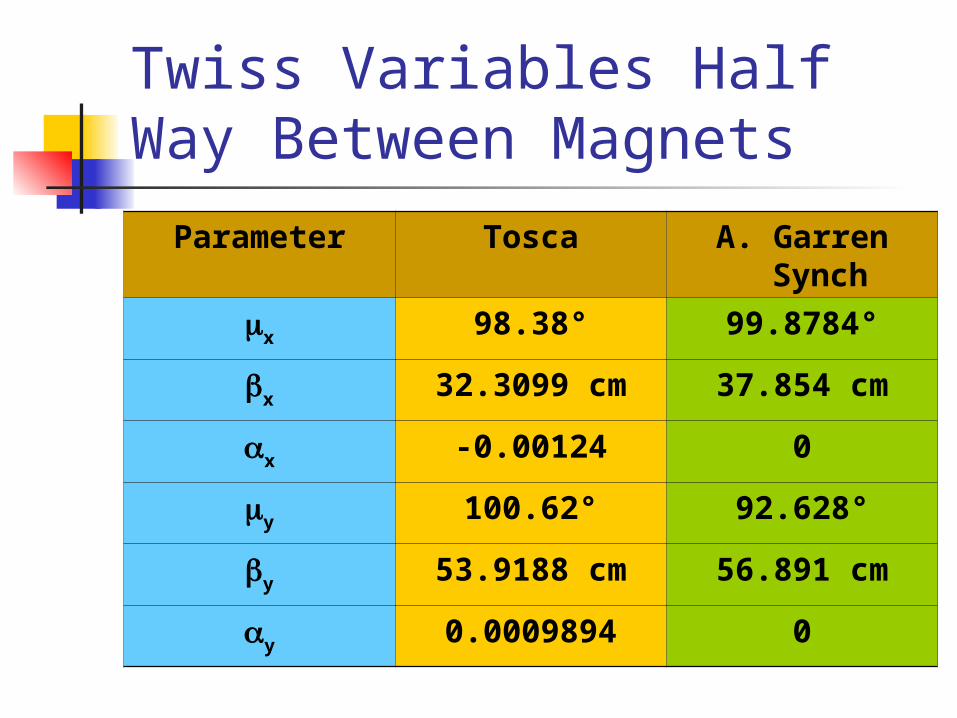
Twiss Variables Half Way Between Magnets
Parameter Tosca A. Garren Synch
x 98.38° 99.8784°
βx 32.3099 cm 37.854 cm
αx -0.00124 0
y 100.62° 92.628°
βy 53.9188 cm 56.891 cm
αy 0.0009894 0
Using the Field Map We can produce a 3D field map from
TOSCA. We could build a GEANT model around this
field map however this has not yet been done.
We have decided that we can provide a field to be used by ICOOL.
ICOOL works in a beam coordinate system. We know the trajectory of the reference path in the
global coordinate system. We can calculate the field and its derivatives
along this path.
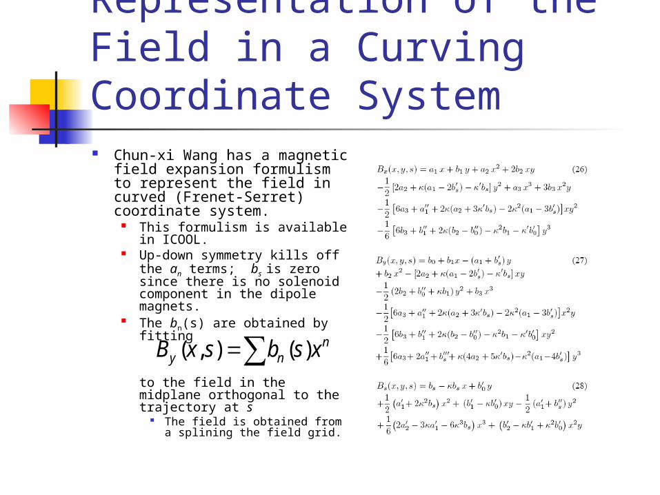
Representation of the Field in a Curving Coordinate System Chun-xi Wang has a magnetic
field expansion formulism to represent the field in curved (Frenet-Serret) coordinate system.
This formulism is available in ICOOL.
Up-down symmetry kills off the an terms; bs is zero since there is no solenoid component in the dipole magnets.
The bn(s) are obtained by fitting
to the field in the midplane orthogonal to the trajectory at s
The field is obtained from a splining the field grid.
nny xsbsxB )(),( ∑=
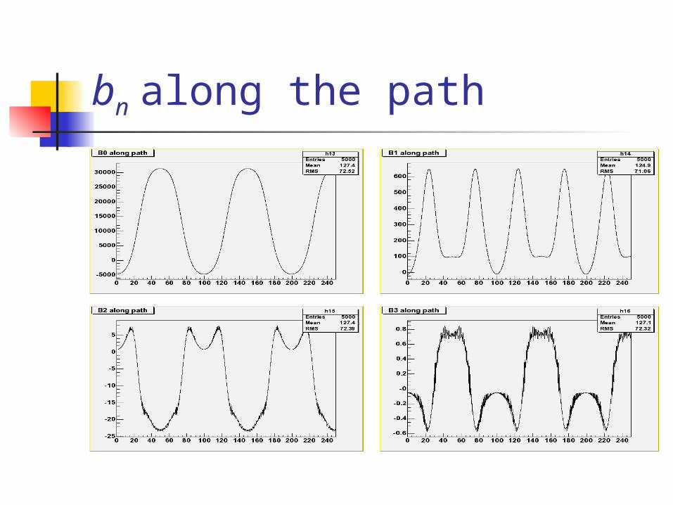
bn along the path
Fourier Expansion of bn(s)
The bn(s) can be expanded with a Fourier series:
These Fourier coefficients can be fed to ICOOL to describe the field with the BSOL 4 option.
We use the bn for n=0 to 5.
T
sikN
knkn ecb
−−
=∑ℜ=
1
0,
T
sik
T
nnk esbT
c )(1
0
, ∫=where
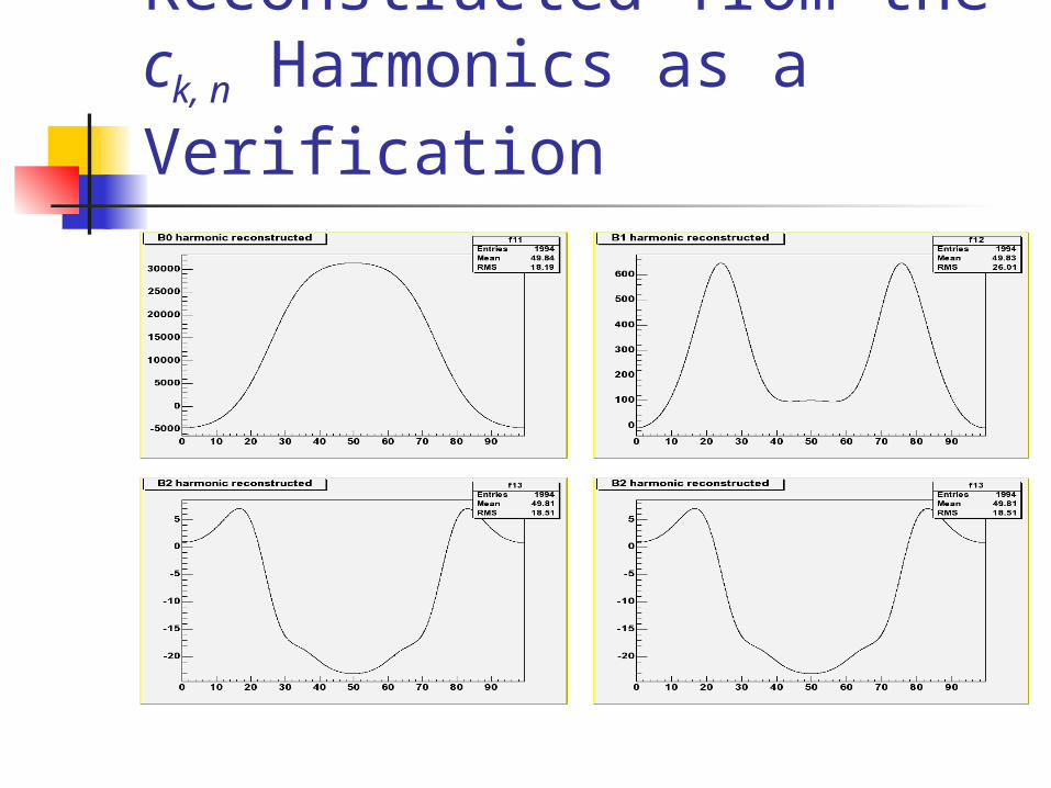
The bn Series Reconstructed from the ck,
n Harmonics as a Verification
Storage Ring Mode Modify Harold Kirk’s ICOOL deck to accept the
Fourier description of the field. Scale the field to 250 MeV/c on the reference orbit.
This is a few percent correction. Verify the configuration in storage ring mode.
RF gradient set to zero. Material density set to zero.
Use a sample of tracks with: x=±1 mm; y=±1 mm; z=±1 mm; px=±10 MeV/c; py=±10 MeV/c; pz= ±10 MeV/c; Also the reference track.
Dynamic Aperture
In order to obtain the dynamic aperture I launched particles at a symmetry point with different start x (y).
The particle position in x vs px (y vs. py) was observed as the particle trajectory crossed the symmetry planes.
I have examined 4 cases: Harold Kirk’s original Hardedge configuration. My Hardedge configuration which tries to duplicate Al
Garren’s lattice My Realistic configuration which tries to duplicate Al
Garren’s lattice. The Realistic configuration ignoring higher order field
components.
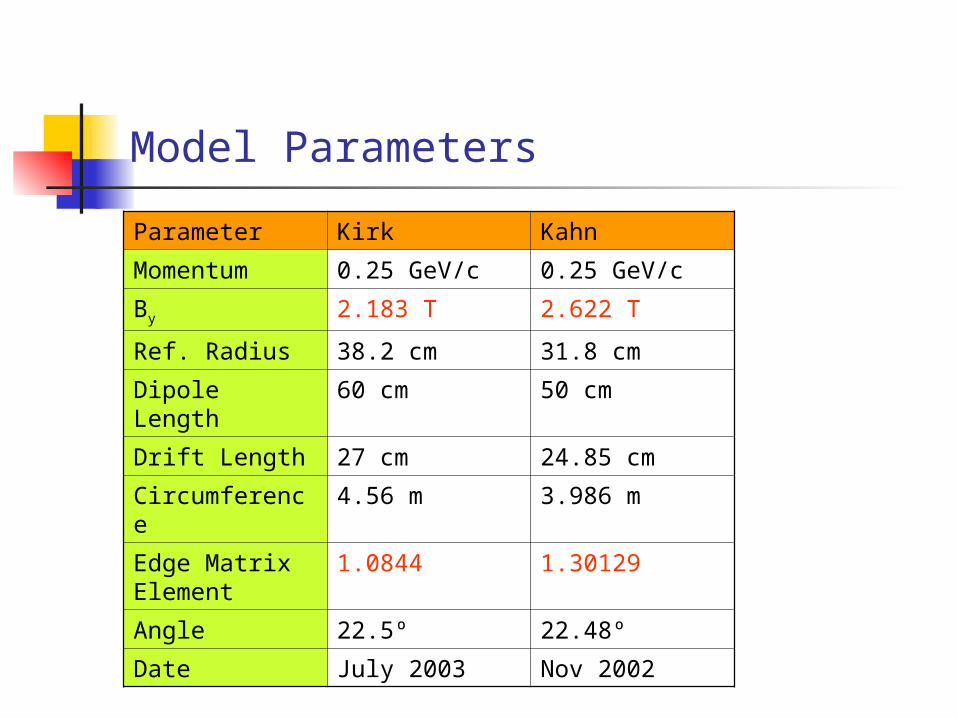
Model Parameters
Parameter Kirk Kahn
Momentum 0.25 GeV/c 0.25 GeV/c
By 2.183 T 2.622 T
Ref. Radius 38.2 cm 31.8 cm
Dipole Length 60 cm 50 cm
Drift Length 27 cm 24.85 cm
Circumference 4.56 m 3.986 m
Edge Matrix Element
1.0844 1.30129
Angle 22.5º 22.48º
Date July 2003 Nov 2002
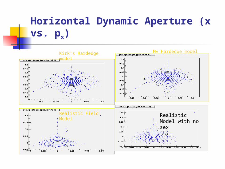
Horizontal Dynamic Aperture (x vs. px)
Kirk’s Hardedge model My Hardedge model
Realistic Field Model Realistic Model with no sex
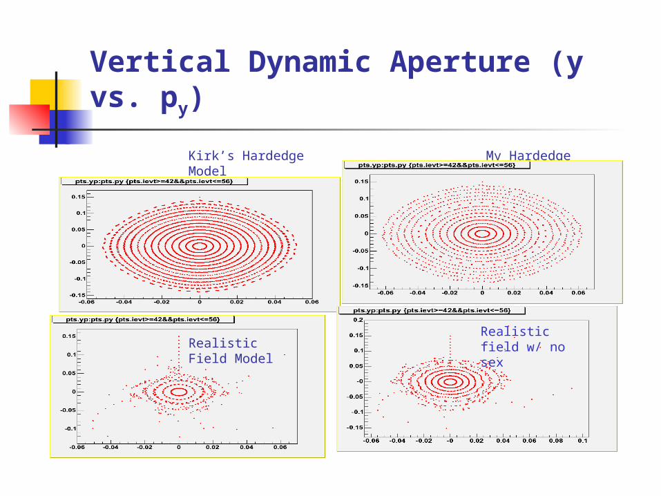
Vertical Dynamic Aperture (y vs. py)
Kirk’s Hardedge Model My Hardedge Model
Realistic Field ModelRealistic field w/ no sex
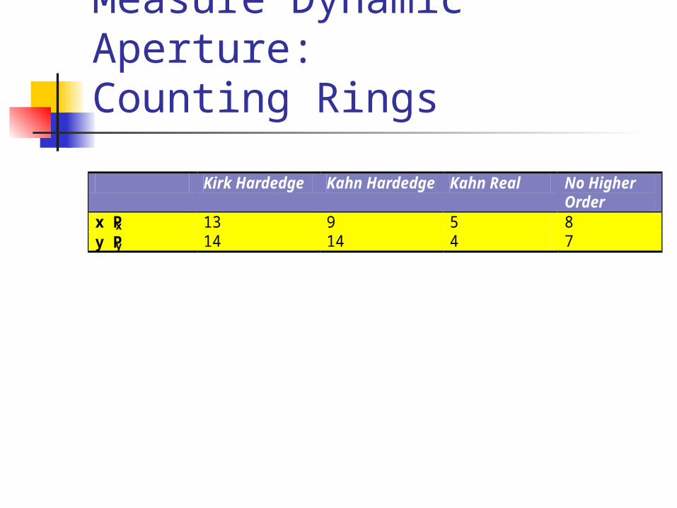
Measure Dynamic Aperture:Counting Rings
Kirk Hardedge Kahn Hardedge Kahn Real No Higher Order
x Px 13 9 5 8 y Py 14 14 4 7
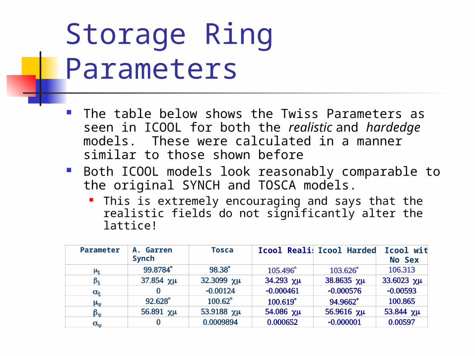
Storage Ring Parameters The table below shows the Twiss Parameters as seen in
ICOOL for both the realistic and hardedge models. These were calculated in a manner similar to those shown before
Both ICOOL models look reasonably comparable to the original SYNCH and TOSCA models. This is extremely encouraging and says that the realistic
fields do not significantly alter the lattice!
Parameter A. Garren Synch
Tosca Icool Realistic Icool Hardedge Icool with No Sex
x 99.8784° 98.38° 105.496° 103.626° 106.313 βx 37.854 cm 32.3099 cm 34.293 cm 38.8635 cm 33.6023 cm αx 0 -0.00124 -0.000461 -0.000576 -0.00593 y 92.628° 100.62° 100.619° 94.9662° 100.865 βy 56.891 cm 53.9188 cm 54.086 cm 56.9616 cm 53.844 cm αy 0 0.0009894 0.000652 -0.000001 0.00597
Conclusion We have shown that for the dipole
cooling ring that hard edge representation of the field can be replaced by a coil description that satisfies Maxwell’s equations. This realistic description maintains the
characteristics of the ring. This realistic description also maintains a
substantial fraction of the dynamic aperture.
Additional Slides
(Since the 2003 Riverside Ring Cooler
Emittance Exchange Workshop)
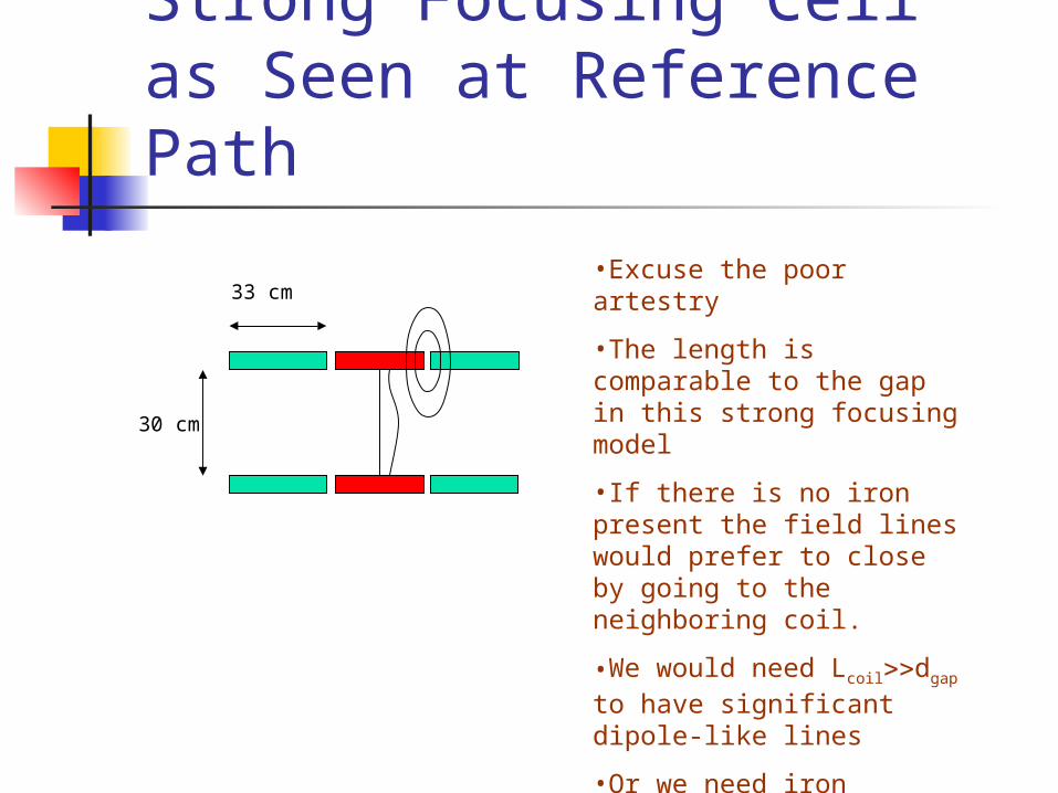
Strong Focusing Cell as Seen at Reference Path
30 cm
33 cm•Excuse the poor artestry
•The length is comparable to the gap in this strong focusing model
•If there is no iron present the field lines would prefer to close by going to the neighboring coil.
•We would need Lcoildgap to have significant dipole-like lines
•Or we need iron
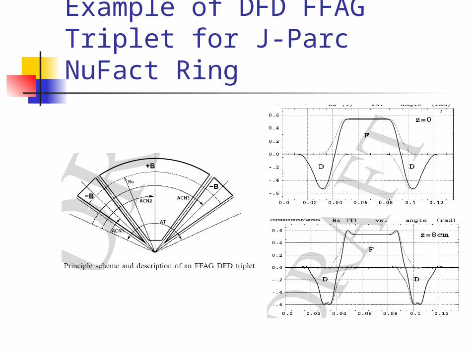
Example of DFD FFAG Triplet for J-Parc NuFact Ring
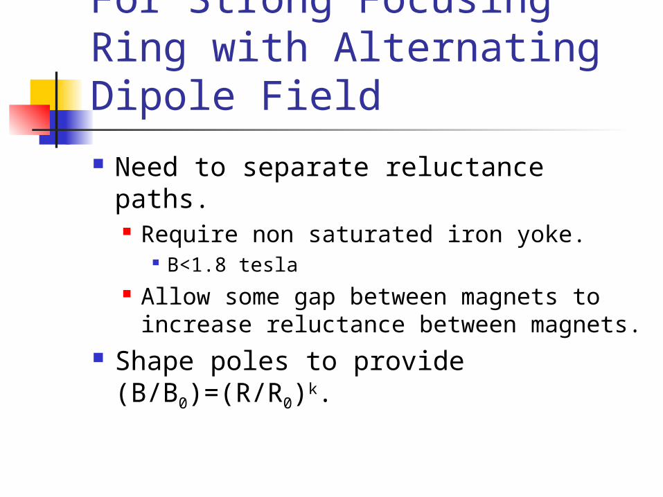
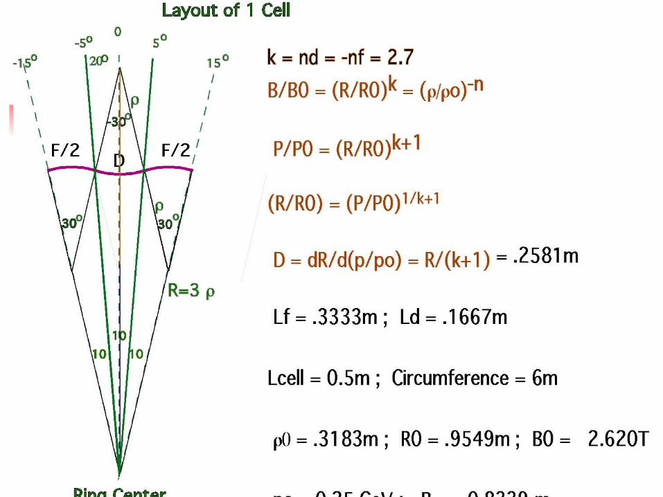
For Strong Focusing Ring with Alternating Dipole Field
Need to separate reluctance paths. Require non saturated iron yoke.
B<1.8 tesla Allow some gap between magnets to
increase reluctance between magnets.
Shape poles to provide (B/B0)=(R/R0)k.


